Bayesian Poisson Tensor Factorization for Inferring Multilateral Relations from Sparse Dyadic Event Counts

Abstract

We present a Bayesian tensor factorization model for inferring latent group structures from dynamic pairwise interaction patterns. For decades, political scientists have collected and analyzed records of the form “country $i$ took action $a$ toward country $j$ at time $t$”—known as dyadic events—in order to form and test theories of international relations. We represent these event data as a tensor of counts and develop Bayesian Poisson tensor factorization to infer a low-dimensional, interpretable representation of their salient patterns. We demonstrate that our model’s predictive performance is better than that of standard non-negative tensor factorization methods. We also provide a comparison of our variational updates to their maximum likelihood counterparts. In doing so, we identify a better way to form point estimates of the latent factors than that typically used in Bayesian Poisson matrix factorization. Finally, we showcase our model as an exploratory analysis tool for political scientists. We show that the inferred latent factor matrices capture interpretable multilateral relations that both conform to and inform our knowledge of international affairs.

1 Introduction

Social processes are characterized by pairwise connections between actors, such as people, organizations, corporations, and countries. In some social processes, actors declare their connections and researchers can directly study them—e.g., friendships on Facebook or co-authorships in academia. In other processes, however, these connections are not explicitly declared. Rather, they are evidenced over time via dynamic interaction patterns. Inferring social processes from such implicit data is a challenging and important task.

This task is especially motivated in international relations. For decades, scholars have collected and analyzed records of pairwise interactions between countries of the form “country $i$ took action $a$ toward country $j$ at time $t$,” known as dyadic events. These data sets, e.g., [28], which are traditionally small and well-curated, help them form and test theories of international relations, which often concern the multilateral behavior of groups of countries. Recently, there has been new interest in studying less structured, larger scale sources of pairwise interaction data. Researchers have created several large data sets, e.g., [20], by automatically extracting and encoding dyadic events from Internet news archives.

These modern data sets differ substantially from their smaller counterparts, which previously dominated the field. Rather than documenting high-level, aggregate behaviors, such as formal wars and military alliances, they document micro-level behaviors at a day-to-day granularity. Although this new view of the world potentially paints a more accurate and nuanced picture of international relations, these data are too noisy and disaggregated to analyze effectively using traditional techniques. We need new methods to uncover the latent multilateral relations that underlie these events.

Figure 1: Our model infers latent components that correspond to multilateral relations. Each component consists of four factor vectors summarizing sender, receiver, action-type, and time-step activity, respectively. Here, we visualize two inferred components. For each component, we plotted the top ten sender, receiver, and action-type factors sorted in decreasing order. We also plotted the entire vector of time-step factors in chronological order. We found that the interpretation of each component was either immediately clear from our existing knowledge or easy to discover via a web search. Left: A component inferred from GDELT data spanning 1990 through 2007 (with monthly time steps) that corresponds to events surrounding the Six Party Talks—a series of diplomatic talks that took place from 2003 through 2009 between South Korea, North Korea, the US, China, Japan, and Russia, aimed at resolving international concerns over North Korea’s nuclear weapons program [37]. The top senders and receivers are the six parties, while the top action types are Consult and Intend to Cooperate. The time-step factors show increased activity beginning in 2003. Right: A component inferred from ICEWS data spanning 1995 through 2012 (with monthly time steps) that corresponds to events surrounding the US-led War on Terror following the September 11, 2001 attacks. The largest time-step factor is that of October 2001—the month during which the invasion of Afghanistan occurred. There is also a blip in August 1998, when the Clinton administration ordered missile attacks on terrorist bases in Afghanistan [33].

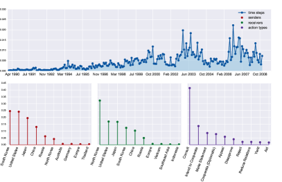
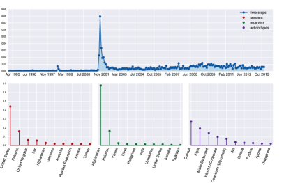
In this paper, we introduce Bayesian Poisson tensor factorization (BPTF) for inferring latent multilateral relations from observed dyadic events. We present a scalable variational inference algorithm and demonstrate our method, via both predictive and exploratory analyses, on large-scale international relations data. Figure 1 illustrates our approach; our model infers both ongoing multilateral relations, such as the Six-Party Talks from 2003 through 2009 (left), as well as relations precipitated by temporally localized anomalous activity, such as the September 11, 2001 attacks (right).

Technical summary:   A data set of dyadic events can be represented as a four-way tensor by aggregating (i.e., counting) events within discrete time steps. Each element of the tensor is a count of the number of actions of type $a$ taken by country $i$ toward country $j$ at time $t$. Our model decomposes such a tensor into a set of latent factor matrices that provide a low-dimensional representation of the salient patterns in the counts—in this case, latent multilateral relations.

Tensors derived from dyadic event data are often very sparse since most countries rarely interact with one another. Additionally, the non-zero counts, for countries that do interact, are highly dispersed—i.e., their mean is greatly exceeded by their variance. Traditional tensor factorization methods, involving maximum likelihood estimation, are unstable when fit to sparse count tensors [2]. Bayesian Poisson tensor factorization (section 3) builds on previous work on Bayesian Poisson matrix factorization with Gamma priors [1, 21, 11, 38, 25, 10] to avoid these instabilities. We validate our model by comparing its out-of-sample predictive performance to non-Bayesian tensor factorization methods (section 5); BPTF significantly outperforms other models when decomposing sparse, highly dispersed count data.

We present an efficient variational inference algorithm to fit BPTF to data (section 4) and outline the relationship between our algorithm and the traditional maximum likelihood approach (section 7). This relationship explains why BPTF outperforms other methods without any sacrifice to efficiency. It also suggests that when constructing point estimates of the latent factors from the variational distribution, researchers should use the geometric expectation instead of the arithmetic expectation commonly used in Bayesian Poisson matrix factorization. We show that using the geometric expectation increases the sparsity of the inferred factors and improves predictive performance. We therefore recommend its use in any subsequent work involving variational inference for Bayesian Poisson matrix or tensor factorization.

Finally, we showcase Bayesian Poisson tensor factorization as an exploratory analysis tool for political scientists (section 6). We demonstrate that the inferred latent factor matrices capture interpretable multilateral relations that conform to and inform our knowledge of international affairs.

2 Dyadic Events

Over the past few years, researchers have created large data sets of dyadic events by automatically extracting them from Internet news archives. The largest of these data sets is the Global Database of Events, Location, and Tone (GDELT), introduced in 2013, which contains over a quarter of a billion events from 1979 to the present, and is updated with new events daily [20]. In parallel, government agencies (e.g., DARPA) and their contractors have also started to collect and analyze dyadic events, in order to forecast political instability and to develop early-warning systems [24]; Lockheed Martin publicly released the Integrated Crisis Early Warning System (ICEWS) database in early 2015. Ward et al. provide a comparison of GDELT and ICEWS [31].

GDELT and ICEWS use the CAMEO coding scheme [6]. A CAMEO-coded dyadic event consists of four pieces of information: a sender, a receiver, an action type, and a timestamp. An example of such an event (top) and a sentence from which it could have been extracted (bottom) is

$$\langle\textrm{Turkey, Syria, \emph{Fight}, }12/25/2014\rangle$$

Dec. 25, 2014: “Turkish jets bombed targets in Syria.”

CAMEO assumes that senders and receivers belong to a single set of actors, coded for their country of origin and sector (e.g., government or civilian) as well as other information (such as religion or ethnicity). CAMEO also assumes a hierarchy of action types, with the top level consisting of twenty basic action classes. These classes are loosely ranked based on sentiment from Make Public Statement to Use Unconventional Mass Violence. Each action class is subdivided into more specific actions; for example, Make Public Statement contains Make Empathetic Comment. When studying international relations using CAMEO-coded data, researchers commonly consider only the countries of origin as actors and only the twenty basic action classes as action types. In ICEWS, there are 249 unique country-of-origin actors (which include non-universally recognized countries, such as Taiwan and Palestine); in GDELT, there are 223.

Dyadic events as tensors:  A data set of dyadic events can be aggregated into a four-way tensor $\boldsymbol{Y}$ of size $N\times N\times A\times T$, where $N$ is the number of country actors and $A$ is the number of action types, by aggregating the events into $T$ time steps on the basis of their timestamps. Each element $y_{ijat}$ of $\boldsymbol{Y}$ is a count of the number of actions of type $a$ taken by country $i$ toward country $j$ during time step $t$. As described in section 6, we experimented with various date ranges and time step granularities. For example, in one set of experiments, we used the entire ICEWS data set, spanning 1995 through 2012 (i.e., 18 years) with monthly time steps—i.e., a $249\times 249\times 20\times 216$ tensor with 267,844,320 elements.

Tensors derived from ICEWS and GDELT are very sparse. For the $249\times 249\times 20\times 216$ ICEWS tensor described above, only 0.54% of the elements (roughly 1.5 million elements) are non-zero. Moreover, these non-zero counts are highly dispersed with a variance-to-mean ratio (VMR) of 57. Any realistic model of such data must therefore be robust to sparsity and capable of representing high levels of dispersion.

3 Bayesian Poisson Tensor
Factorization

Tensor factorization methods decompose an observed $M$-way tensor $\boldsymbol{Y}$ into $M$ latent factor matrices $\Theta^{(1)},\ldots,\Theta^{(M)}$ that provide a low-dimensional representation of the salient patterns in $\boldsymbol{Y}$. There are many different tensor factorization methods; the two most common methods are the Tucker decomposition [30] and the Canonical Polyadic (CP) decomposition [13]. These methods can both be viewed as tensor generalizations of singular value decomposition. Here, we focus on the CP decomposition, as it performs better than the Tucker decomposition when modeling sparse count data [18].

For a four-way count tensor $\boldsymbol{Y}$ of size $N\times N\times A\times T$, the CP decomposition treats each observed count $y_{ijat}$ as

$$y_{ijat}\approx\hat{y}_{ijat}\equiv\sum_{k=1}^{K}\theta^{(1)}_{ik}\theta^{(2)}_{jk}\theta^{(3)}_{ak}\theta^{(4)}_{tk}$$ (1)

for $i,j\in[N]$, $a\in[A]$, and $t\in[T]$, where $\theta^{(1)}_{ik}$, $\theta^{(2)}_{jk}$, $\theta^{(3)}_{ak}$, and $\theta^{(4)}_{tk}$ are known as factors, $\hat{y}_{ijat}$ is known as the reconstruction of count $y_{ijat}$, and $\hat{\boldsymbol{Y}}$ is the reconstruction of the entire tensor $\boldsymbol{Y}$. The set of all factors used to model $\boldsymbol{Y}$ can be aggregated into four latent factor matrices; for example, $\Theta^{(1)}\equiv\big{(}\big{(}\theta^{(1)}_{ik}\big{)}_{i=1}^{N}\big{)}_{k=1}^{K}$—an $N\times K$ matrix. Since each factor matrix has $K$ columns, a single index $k\in[K]$ indexes four columns (one per matrix). These columns are collectively known as a component; for example, component $k$ consists of $\big{(}\theta^{(1)}_{ik}\big{)}_{i=1}^{N}$, $\big{(}\theta^{(2)}_{jk}\big{)}_{j=1}^{N}$, $\big{(}\theta_{ak}^{(3)}\big{)}_{a=1}^{A}$, and $\big{(}\theta_{tk}^{(4)}\big{)}_{t=1}^{T}$—i.e., a length-$N$ vector of sender factors, a length-$N$ vector of receiver factors, a length-$A$ vector of action-type factors, and a length-$T$ vector of time-step factors. Figure 1 visually depicts two components inferred from ICEWS and GDELT.

When viewed from a probabilistic perspective, the reconstruction $\hat{y}_{ijat}\equiv\sum_{k=1}^{K}\theta_{ik}^{(1)}\theta_{jk}^{(2)}\theta_{ak}^{(3)}\theta_{tk}^{(4)}$ can be thought of as the mean of the distribution from which the observed count $y_{ijat}$ is assumed to have been drawn. If this distribution is a Poisson—i.e., if $y_{ijat}\sim\textrm{Pois}(y_{ijat};\hat{y}_{ijat})$—then the process of decomposing $\boldsymbol{Y}$ into its latent factor matrices is known as Poisson tensor factorization (PTF), and can be performed via maximum likelihood estimation (MLE) of $\Theta^{(1)}$, $\Theta^{(2)}$, $\Theta^{(3)}$, and $\Theta^{(4)}$. For sparse count data, PTF often yields better estimates of the latent factor matrices than those obtained by assuming each count to have been drawn from a Gaussian distribution—i.e., $y_{ijat}\sim\mathcal{N}(y_{ijat};\hat{y}_{ijat},\sigma^{2})$ [2].

In this paper, we also assume that each observed count $y_{ijat}$ is drawn from a Poisson distribution with mean $\hat{y}_{ijat}$; however, rather than obtaining point estimates of the factor matrices using maximum likelihood estimation, we impose prior distributions on the latent factors and perform full Bayesian inference. Bayesian inference for Poisson matrix factorization (PMF) was originally proposed by Cemgil [1] and has been successfully used for several tasks including image reconstruction [1], music tagging [21], topic modeling [25], content recommendation [11], and community detection [9]; here, we generalize Bayesian PMF to tensors.

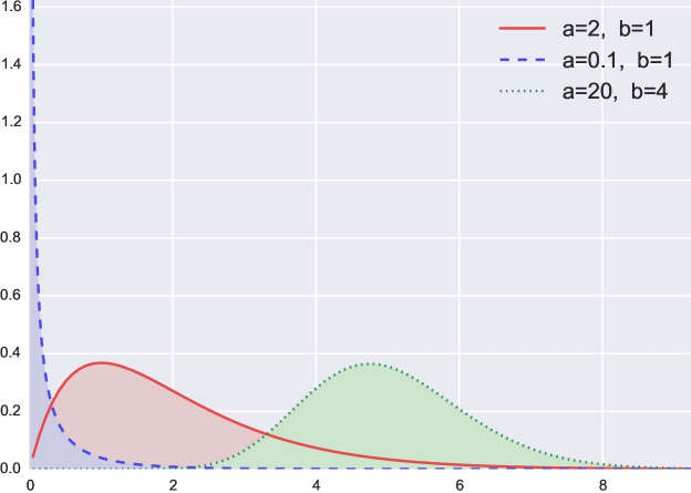
Since the Gamma distribution is the conjugate prior for a Poisson likelihood, Bayesian PMF typically imposes Gamma priors on the latent factors [1, 11, 39]. The Gamma distribution, which has support on $(0,\infty)$, is parameterized by a shape parameter $a>0$ and a rate parameter $b>0$; if $\theta\sim\textrm{Gamma}\,(\theta;a,b)$, then $\mathbb{E}[\theta]=\frac{a}{b}$ and $\textrm{Var}[\theta]=\frac{a}{b^{2}}$. Thus, when $a\ll 1$ and $b$ is small, the Gamma distribution concentrates most of its mass near zero yet maintains a heavy tail and can therefore be used as a sparsity-inducing prior [1, 11]. We show the effects of different $a$ and $b$ values in figure 2.

Figure 2: Three Gamma distributions with different values for the shape $a$ and rate $b$ parameters. The distribution induces sparsity when $a\ll 1$ and $b$ is small (shown in blue).

To define Bayesian Poisson tensor factorization (BPTF) for a four-way tensor, we impose four sparsity-inducing Gamma priors over the latent factors. For a single factor, e.g., $\theta^{(1)}_{ik}$,

$$\theta^{(1)}_{ik}\sim\textrm{Gamma}\,(\theta^{(1)}_{ik};\alpha,\alpha\,\beta^{(1)}),$$ (2)

and similarly for $\theta^{(2)}_{jk}$, $\theta^{(3)}_{ak}$, and $\theta^{(4)}_{tk}$. Under this parameterization of the Gamma distribution, where the rate parameter is the product of the shape parameter and $\beta^{(1)}$, the mean of the prior is completely determined by $\beta^{(1)}$ (since $\mathbb{E}[\theta_{ik}^{(1)}]=\frac{\alpha}{\alpha\beta^{(1)}}=\frac{1}{\beta^{(1)}}$), which can be inferred from the data [1, 21]. The shape parameter $\alpha$, which determines the sparsity of the latent factor matrices, can be set by the user. Throughout our experiments, we use $\alpha=0.1$ to encourage sparsity and hence promote interpretability of the factors.

4 Variational inference

Given an observed tensor $\boldsymbol{Y}$, Bayesian inference of the latent factors involves “inverting” the generative process described in the previous section to obtain the posterior distribution of the latent factor matrices conditioned on $\boldsymbol{Y}$ and the model hyperparameters $\mathcal{H}\equiv\{\alpha,\beta^{(1)},\beta^{(2)},\beta^{(3)},\beta^{(4)}\}$:

$$P\left(\Theta^{(1)},\Theta^{(2)},\Theta^{(3)},\Theta^{(4)}\,|\,\mathbf{Y},\mathcal{H}\right).$$

The posterior distribution for BPTF is analytically intractable and must be approximated. Variational inference turns the process of approximating the posterior distribution into an optimization algorithm. It involves first specifying a parametric family of distributions $Q$ over the latent variables of interest, indexed by the values of a set of variational parameters $\mathcal{S}$. The functional form of $Q$ is typically chosen so as to facilitate efficient optimization of $\mathcal{S}$. Here, we use a fully factorized mean-field approximation and define $Q$ to be the product of $N\cdot N\cdot A\cdot T\cdot K$ independent Gamma distributions—one for each latent factor—e.g., for $\theta_{ik}^{(1)}$,

$$Q(\theta^{(1)}_{ik};\mathcal{S}^{(1)}_{ik})=\textrm{Gamma}\,(\theta^{(1)}_{ik};\gamma^{(1)}_{ik},\delta^{(1)}_{ik}),$$ (3)

where $\mathcal{S}^{(1)}\equiv\big{(}\big{(}\gamma^{(1)}_{ik},\delta^{(1)}_{ik}\big{)}_{i=1}^{N}\big{)}_{k=1}^{K}$. The full set of variational parameters is thus $\mathcal{S}\equiv\{\mathcal{S}^{(1)},\mathcal{S}^{(2)},\mathcal{S}^{(3)},\mathcal{S}^{(4)}\}$. This form of $Q$ is similar to that used in Bayesian PMF [1, 25, 11].

The variational parameters are then fit so as to yield the closest member of $Q$ to the exact posterior—known as the variational distribution. Specifically, the algorithm sets the values of $\mathcal{S}$ to those that minimize the KL divergence of the exact posterior from $Q$. It can be shown that these values are the same as those that maximize a lower bound on $P(\boldsymbol{Y}\,|\,\mathcal{H})$, known as the evidence lower bound (ELBO):

$$\mathcal{B}(\mathcal{S})=\mathbb{E}_{Q}\left[\log{\left(P(\boldsymbol{Y},\Theta^{(1)},\Theta^{(2)},\Theta^{(3)},\Theta^{(4)}\,|\,\mathcal{H})\right)}\right]+H(Q),$$

where $H(Q)$ is the entropy of $Q$. When $Q$ is a fully factorized approximation, finding values of $\mathcal{S}$ that maximize the ELBO can be achieved by performing coordinate ascent, iteratively updating each variational parameter, while holding the others fixed, until convergence (defined by relative change in the ELBO). The update equation for each parameter can be derived easily using an auxiliary variable as shown for Bayesian PMF [1, 25, 11]; we therefore omit derivations.

For parameters $\gamma^{(1)}_{ik}$ and $\delta^{(1)}_{ik}$, the update equations are

$$\gamma^{(1)}_{ik} :=\alpha+\sum_{j,a,t}y_{ijat}\frac{\mathbb{G}_{Q}\left[\theta^{(1)}_{ik}\theta^{(2)}_{jk}\theta^{(3)}_{ak}\theta^{(4)}_{tk}\right]}{\sum_{k=1}^{K}\mathbb{G}_{Q}\left[\theta^{(1)}_{ik}\theta^{(2)}_{jk}\theta^{(3)}_{ak}\theta^{(4)}_{tk}\right]}$$ (4)

$$\delta^{(1)}_{ik} :=\alpha\,\beta^{(1)}+\sum_{j,a,t}\mathbb{E}_{Q}\left[\theta^{(2)}_{jk}\theta^{(3)}_{ak}\theta^{(4)}_{tk}\right],$$ (5)

where $\mathbb{E}_{Q}\left[\cdot\right]$ and $\mathbb{G}_{Q}\left[\cdot\right]=\exp{(\mathbb{E}_{Q}\left[\log{(\cdot)}\right])}$ denote arithmetic and geometric expectations. Since $Q$ is fully factorized, each expectation of a product can be factorized into a product of individual expectations, which, e.g., for $\theta_{ik}^{(1)}$ are

$$\mathbb{E}_{Q}\left[\theta^{(1)}_{ik}\right]=\frac{\gamma^{(1)}_{ik}}{\delta^{(1)}_{ik}}\quad\textrm{and}\quad\mathbb{G}_{Q}\left[\theta^{(1)}_{ik}\right]=\frac{\exp\big{(}\Psi\big{(}\gamma^{(1)}_{ik}\big{)}\big{)}}{\delta^{(1)}_{ik}},$$ (6)

where $\Psi(\cdot)$ is the digamma function. Each expectation—a sufficient statistic—can be cached to improve efficiency. Note that the summand in (4) need only be computed for those values of $j$, $a$, and $t$ for which $y_{ijat}>0$; provided $\boldsymbol{Y}$ is very sparse, inference is efficient even for very large tensors.

The hyperparameters $\beta^{(1)}$, $\beta^{(2)}$, $\beta^{(3)}$, and $\beta^{(4)}$ can be optimized via an empirical Bayes method, in which each hyperparameter is iteratively updated along with the variational parameters according to the following update equation:

$$\beta^{(1)}:=\left(\sum_{i,k}\mathbb{E}_{Q}\left[\theta_{ik}^{(1)}\right]\right)^{-1}.$$ (7)

Update equations (4), (5), and (7) completely specify the variational inference algorithm for BPTF. Our Python implementation, which is intended to support arbitrary $M$-way tensors in addition to the four-way tensors described in this paper, is available for use under an open source license.

5 Predictive Analysis

Table 1: Out-of-sample predictive performance for our model (BPTF) and non-negative tensor factorization with Euclidean distance (NTF-LS) and generalized KL divergence (NTF-KL or, equivalently, PTF). Each row contains the results of a single experiment. “I-top-25” means the experiment used data from ICEWS and we predicted the upper-left $25\times 25$ portion of each test slice (and treated its complement as observed). “G-top-100^c” means the experiment used data from GDELT and we predicted the complement of the upper-left $100\times 100$ portion of each test slice. For each experiment, we state the density (percentage of non-zero elements) and VMR (i.e., dispersion) of the unobserved portion of the test set. We report three types of error: mean absolute error (MAE), mean absolute error on non-zero elements (MAE-NZ), and Hamming loss on the zero elements (HAM-Z). All models achieved comparable scores when we predicted the sparser portion of each test slice (bottom four rows). BPTF significantly outperformed the other models when we predicted the denser $25\times 25$ or $100\times 100$ portion (top four rows).

			NTF-LS			NTF-KL (PTF)			BPTF
	Density	VMR	MAE	MAE-NZ	HAM-Z	MAE	MAE-NZ	HAM-Z	MAE	MAE-NZ	HAM-Z
I-top-25	0.1217	105.8755	34.4	217	0.271	8.37	56.7	0.138	1.99	12.9	0.113
G-top-25	0.2638	180.4143	52.5	167	0.549	15.5	53.7	0.327	8.94	29.8	0.292
I-top-100	0.0264	63.1118	29.8	979	0.0792	10.5	346	0.0333	0.178	5.05	0.0142
G-top-100	0.0588	111.8676	42.6	470	0.217	4	58.6	0.0926	0.95	12.2	0.0682
I-top-25c	0.0021	8.6302	0.00657	2.27	0.00023	0.0148	2.72	0.00256	0.0104	2.31	0.00161
G-top-25c	0.0060	20.4858	0.0435	4.4	0.00474	0.0606	4.9	0.00893	0.0412	4.01	0.00601
I-top-100c	0.0004	4.4570	0.000685	1.63	3.33e-07	0.0011	1.55	5.43e-05	0.00109	1.56	4.97e-05
G-top-100c	0.0015	9.9432	0.00584	3.23	0.000112	0.0084	2.97	0.00109	0.00803	3	0.000957

We validated our model by comparing its predictive performance to that of standard methods for non-negative tensor factorization involving maximum likelihood estimation.

Baselines:  Non-Bayesian methods for CP decomposition find values of the latent factor matrices that minimize some cost function of the observed tensor $\boldsymbol{Y}$ and its reconstruction $\hat{\boldsymbol{Y}}$. Researchers have proposed many cost functions, but most often use Euclidean distance or generalized KL divergence, preferring the latter when the observed tensor consists of sparse counts. Generalized KL divergence is

$$D(\boldsymbol{Y}\,||\,\hat{\boldsymbol{Y}})=-\sum_{i,j,a,t}\left(y_{ijat}\log{(\hat{y}_{ijat})}-\hat{y}_{ijat}\right)+C,$$ (8)

where constant $C\equiv\sum_{i,j,a,t}\left(y_{ijat}\log{(y_{ijat})}-y_{ijat}\right)$ depends on the observed data only. The standard method for estimating the values of the latent factors involves multiplicative update equations, originally introduced for matrix factorization by Lee and Seung [19] and later generalized to tensors by Welling and Weber [32]. The multiplicative nature of these update equations acts as a non-negativity constraint on the factors which promotes interpretability and gives the algorithm its name: non-negative tensor factorization (NTF).

Figure 3: Sender–receiver slices from the GDELT tensor spanning 1990 through 2007, with monthly time steps (i.e., $T=216$). Both slices correspond to $t=151$ (July 2002). The left slice corresponds to Intend to Cooperate, while the right slice corresponds to Threaten. We sorted the country actors by their overall activity so that the slices were generally denser toward the upper-left corner; only the upper-left $35\times 35$ portion of each slice is shown here. The three darkest elements (i.e., highest counts) in the second slice correspond to Israel $\rightarrow$ Palestine, Palestine $\rightarrow$ Israel, and US $\rightarrow$ Iraq.

Some cost functions also permit a probabilistic interpretation: finding values of the latent factors that minimize them is equivalent to maximum likelihood estimation of a probabilistic model. The log likelihood function of a Poisson tensor factorization model—$y_{ijat}\sim\textrm{Pois}(y_{ijat};\hat{y}_{ijat})$—is

$$\mathcal{L}(\hat{\boldsymbol{Y}};\boldsymbol{Y}) =\log{\left(\prod_{i,j,a,t}\frac{(\hat{y}_{ijat})^{y_{ijat}}}{y_{ijat}!}\exp{\left(-\hat{y}_{ijat}\right)}\right)}$$ (9)

$$=\sum_{i,j,a,t}\left(y_{ijat}\log{(\hat{y}_{ijat})}-\hat{y}_{ijat}\right)+C,$$ (10)

where constant $C\equiv\sum_{i,j,a,t}-\log{\left(y_{ijat}!\right)}$ depends on the observed data only. Since equation (8) is equal to the negative of equation (10) up to a constant, maximum likelihood estimation for Poisson tensor factorization is equivalent to minimizing the generalized KL divergence of $\hat{\boldsymbol{Y}}$ from $\boldsymbol{Y}$.

To validate our modeling assumptions, we compared the out-of-sample predictive performance of BPTF to that of non-negative tensor factorization with Euclidean distance (NTF-LS) and non-negative tensor factorization with generalized KL divergence (NTF-KL or, equivalently PTF).

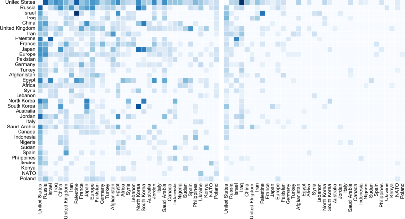
Experimental design:  Using both ICEWS and GDELT, we explored how well each model generalizes to out-of-sample data with varying degrees of sparsity and dispersion. For each data set—ICEWS or GDELT—we sorted the country actors by their overall activity (as both sender and receiver) so that the $N\times N$ sender–receiver slices of the observed tensor were denser toward the upper-left corner. Figure 3 depicts this property. We then divided the observed tensor into a training set and a test set by randomly constructing an 80%–20% split of the time steps. We defined training set $\boldsymbol{Y}^{\text{train}}$ to be the $N\times N\times A$ slices of $\boldsymbol{Y}$ indexed by the time steps in the 80% split and defined test set $\boldsymbol{Y}^{\textrm{test}}$ to be the $N\times N\times A$ slices indexed by the time steps in the 20% split.

We compared the models’ predictive performance in two scenarios, intended to test their abilities to handle different levels of sparsity and dispersion: one in which we treated the denser upper-left $N^{\prime}\times N^{\prime}$ (for some $N^{\prime}<N$) portion of each test slice as observed at test time and predicted its complement, and one in which we observed the complement at test time and predicted the denser $N^{\prime}\times N^{\prime}$ portion.

In each setting, we used an experimental strategy analogous to strong generalization for collaborative filtering [23]. During training, we fit each model to the fully observed training set. We then fixed the values of the variational parameters for the sender, receiver, and action-type factor matrices (or direct point estimates of the factors, for the non-Bayesian models) to those inferred from the training set. For each test slice, indexed by time step $t$, we used the observed upper-left $N^{\prime}\times N^{\prime}$ portion (or its complement) to infer variational parameters for (or direct point estimates of) its time-step factors $\{\theta_{tk}^{(4)}\}_{k=1}^{K}$. Finally, we reconstructed the missing portion of each test slice using equation (1). For the reconstruction step, we can obtain point estimates of the latent factors by taking their arithmetic expectations or their geometric expectations under the variational distribution. In this section, we report results obtained using geometric expectations only; we explain this choice in section 7.

Figure 4: Regional relations between Central Asian republics and regional superpowers, found in both GDELT (left; spanning 1990 through 2007, with monthly time steps) and ICEWS (right; spanning 1995 through 2012, with monthly time steps).

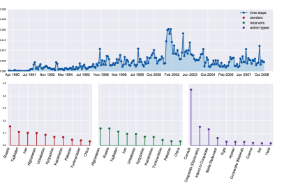
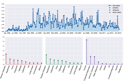
The time-step factors inferred from the observed portion of a given test slice capture the extent to which the sender, receiver, and action-type factors for each component inferred from the training set describe (the observed portion of) that slice. For example, if component $k$ summarizes the Israeli–Palestinian conflict, with Israel and Palestine as top actors and Fight as a top action type, then if Israeli–Palestinian hostilities were intense during test time step $t$ and if Israel and Palestine belong to the observed portion of each test slice, the inferred value of $\theta^{(4)}_{tk}$ is very likely to be large.

We used the entire ICEWS data set from 1995 through 2012 (i.e., 18 years), with events aggregated into monthly time steps. The resultant tensor was of size $249\times 249\times 20\times 216$. Since GDELT covers a larger date range (1979 to the present) than ICEWS, we therefore selected an 18-year subset of GDELT spanning 1990 through 2007, and aggregated events into monthly time steps to yield a tensor of size $223\times 223\times 20\times 216$. Since we are interested in interactions between countries, we omitted self-actions so that the diagonal of each $N\times N$ sender–receiver slice was zero. Ranking the country actors by their overall activity (as both sender and receiver), the top four actors in the ICEWS tensor are USA, Russia, China, and Israel, while the top four actors in the GDELT tensor are USA, Russia, Israel, and Iraq. The GDELT tensor contains many more events than the ICEWS tensor (26 million events versus six million events). It is also much denser (1.6% of the elements are non-zero, as opposed to 0.54%) and exhibits a much higher level of dispersion (VMR of 100, as opposed to 57).

Summary of results:  The out-of-sample predictive performance of each model is shown in table 1. We experimented with several different values of $K$ and found that all three models were insensitive to its value; we therefore report only those results obtained using $K=50$. We computed three types of error: mean absolute error (MAE), mean absolute error on only non-zero elements (MAE-NZ), and Hamming loss on only the zero elements (HAM-Z). HAM-Z corresponds to the fraction of true zeros in the unobserved portion of the test set (i.e., elements for which $y_{ijat}=0$) whose reconstructions were (incorrectly) predicted as being greater than 0.5. For each data set, we generated three training–test splits, and averaged the error scores for each model across them. For each experiment included in table 1, we display the density and dispersion of the corresponding test set. When we treated the dense upper-left $N^{\prime}\times N^{\prime}$ portion as observed at test time (and predicted its complement), all models performed comparably. In this scenario, NTF-LS consistently achieved the lowest MAE score and the lowest HAM-Z score, but not the lowest MAE-NZ score. This pattern suggests that NTF-LS overfits the sparsity of the training set: when the unobserved portion of the test set is much sparser than the training set (as it is in this scenario), NTF-LS achieves lower error scores by simply predicting many more zeros than NTF-KL (i.e., PTF) or BPTF. In the opposite scenario, when we observed the complement at test time and predicted the denser $N^{\prime}\times N^{\prime}$ portion, NTF-LS produced significantly worse predictions than the other models, and our model (BPTF) achieved the lowest MAE, MAE-NZ, and HAM-Z scores—in some cases by an order of magnitude over NTF-KL. These results suggest that in the presence of sparsity, BPTF is a much better model for the “interesting” portion of the tensor—i.e., the dense non-zero portion. This observation is consistent with previous work by Chi and Kolda which demonstrated that NTF can be unstable, particularly when the observed tensor is very sparse [2]. In section 7, we provide a detailed discussion comparing NTF and BPTF, and explain why BPTF overcomes the sparsity-related issues often suffered by NTF.

6 Exploratory Analysis

In this section, we focus on the interpretability of the latent components inferred using our model. (Recall that each latent factor matrix has $K$ columns; a single index $k\in[K]$ indexes a column in each matrix—$\big{(}\theta_{ik}^{(1)}\big{)}_{i=1}^{N}$, $\big{(}\theta_{jk}^{(2)}\big{)}_{j=1}^{N}$, $\big{(}\theta_{ak}^{(3)}\big{)}_{a=1}^{A}$, and $\big{(}\theta_{tk}^{(4)}\big{)}_{t=1}^{T}$—collectively known as a component.) We used our model to explore data from GDELT and ICEWS with several date ranges and time step granularities, including the 18-year, monthly-time-step tensors described in the previous section (treated here as fully observed).

When inferring factor matrices from data that span a large date range (e.g., 18 years), we expect that the inferred components will correspond to multilateral relations that persist or recur over time. Figure 1 shows two such components, inferred from the 18-year GDELT and ICEWS tensors. The first component corresponds to ongoing negotiations over North Korea’s nuclear program, while the second corresponds to a decade-long war (though precipitated by a sudden anomalous event). We found that many the components inferred from 18-year tensors summarize regional relations—i.e., multilateral relations that persist due to geographic proximity—similar to those found by Hoff [15].

Figure 5: Left: Three Japanese citizens were taken hostage in Iraq during April 2004 and a third was found murdered in October 2004 [35]. This component inferred from GDELT (2004 through 2005, weekly time steps) had the sparsest time-step factor vector. We performed a web search for japan iraq april 2004 to interpret this component. Right: Protests erupted in Islamic countries after a Danish newspaper published cartoons depicting the Prophet Muhammad [36]. Denmark and Iran cut diplomatic ties in February 2006 after protesters attacked the Danish embassy in Tehran. This component inferred from GDELT (2006 through 2007, weekly time steps) had the second sparsest time-step factor vector. Web search: denmark iran january 2006.

We found a high correspondence between the regional components inferred from GDELT and the regional components inferred from ICEWS, despite the five-year difference in their date ranges. Figure 4 illustrates this correspondence. We also found that components summarizing regional relations exhibited the least sparsity in their sender, receiver, and time-step factors. For example, the component depicted in figure 4 has near-uniform values for the top ten sender and receiver actors (all of whom are regional to Central Asia), while the time-step factors possess high activity throughout. In contrast, the time-step factors for the component shown in the second plot of figure 1 (i.e., the War on Terror) exhibit a major spike in October 2001. This component’s sender and receiver factors also exhibit uneven activity over the top ten actors, with the US, Afghanistan, and Pakistan dominating.

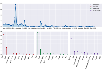
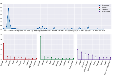
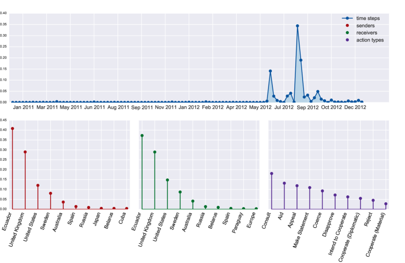
These “regional relations” components conform to our understanding of international affairs and foster confidence in BPTF as an exploratory analysis tool. However, for the same reason, they are also less interesting. To explore temporally localized multilateral relations—i.e., anomalous interaction patterns that do not simply reflect usual activity—we used our model to infer components from several subsets of GDELT and ICEWS, each spanning a two-year date range with weekly time steps. We ranked the inferred components by the sparsity of their time-step factors, measured using the Gini coefficient [3]. Ranking components by their Gini coefficients is a form of anomaly detection: components with high Gini coefficients have unequal time-step factor values—i.e., dramatic spikes. Figure 6 shows the highest-ranked (i.e., most anomalous) component inferred from a subset of GDELT spanning 2011–2012. This component features an unusual group of top actors and a clear burst of activity around June 2012. To interpret this component, we performed a web search for ecuador UK sweden june 2012 and found that the top hit was a Wikipedia page [34] about Julian Assange, the editor-in-chief of the website WikiLeaks—an Australian national, wanted by the US and Sweden, who sought political asylum at the Ecuadorian embassy in the UK during June through August 2012. These countries are indeed the top actors for this component, while the time-step factors and top action types (i.e., Consult, Aid, and Appeal) track the dates and nature of the reported events.

In general, we found that when our existing knowledge was insufficient to interpret an inferred component, performing a web search for the top two-to-four actors along with the top time step resulted in either a Wikipedia page or a news article that provided an explanation. We present further examples of the most anomalous components inferred from other two-year date ranges in figure 5, along with the web searches that we performed in order to interpret them.

Figure 6: Julian Assange, editor-in-chief of WikiLeaks, sought asylum at the Ecuadorian embassy in the UK during June through August 2012. This component inferred from GDELT (2011 through 2012, with weekly time steps) had the sparsest time-step factor vector. We performed a web search for ecuador UK sweden june 2012 to interpret this component.

Figure 7: The mode, arithmetic expectation, and geometric expectation of a Gamma-distributed random variable $\theta$. First: The three quantities for different values of shape $a\geq 1$ (x axis) with rate $b=0.5$. All three grow linearly with $a$ and $\mathbbm{E}\left[\theta\right]\geq\mathbbm{G}\left[\theta\right]\geq\text{Mode}\,(\theta)$. Second: Geometric and arithmetic expectations for different values of shape $a\in(0,1)$, where the mode is undefined, with rate $b=0.5$. $\mathbbm{G}\left[\theta\right]$ grows more slowly than $\mathbbm{E}\left[\theta\right]$. This property is most apparent when $a<0.4$. Third: pdf of a Gamma distribution with shape $a=10$ and rate $b=0.5$. The three quantities are shown as vertical lines. All three are close in the area of highest density, differing by about a half unit of inverse rate, i.e., $\frac{1}{2b}=1$. Fourth: pdf of a Gamma distribution with $a=0.3$ and $b=0.5$. The geometric and arithmetic expectations are shown as vertical lines (the mode is undefined). The two quantities differ greatly, with $\mathbbm{G}\left[\theta\right]$ much closer to zero and in an area of higher density. If these expectations were used as point estimates to predict the presence or absence of a rare event—e.g., $y=0$ if $\hat{\theta}<0.5$; otherwise $y=1$—they would yield different predictions.

7 Technical Discussion

Previous work on Bayesian Poisson matrix factorization (e.g., [1, 25, 11]) presented update equations for the variational parameters in terms of auxiliary variables, known as latent sources, and made no explicit reference to geometric expectations. In contrast, we write the update equations for Bayesian Poisson tensor factorization in the form of equations (4) and (5) in order to highlight their relationship to Lee and Seung’s multiplicative updates for non-negative tensor factorization—a parallel also drawn by Cemgil in his paper introducing Bayesian PMF [1]—and to show that our update equations suggest a new way of making out-of-sample predictions when using BPTF. In this section, we provide a discussion of these connections and their implications.

When performing NTF by minimizing the generalized KL divergence of reconstruction $\hat{\boldsymbol{Y}}$ from observed tensor $\boldsymbol{Y}$ (which is equivalent to MLE for PTF), the multiplicative update equation introduced by Lee and Seung for, e.g., $\theta^{(1)}_{ik}$ is

$$\theta^{(1)}_{ik}:=\theta^{(1)}_{ik}\frac{\sum_{j,a,t}\theta^{(2)}_{jk}\theta^{(3)}_{ak}\theta^{(4)}_{tk}\,\frac{y_{ijat}}{\hat{y}_{ijat}}}{\sum_{j,a,t}\theta^{(2)}_{jk}\theta^{(3)}_{ak}\theta^{(4)}_{tk}}.$$ (11)

These update equations sometimes converge to locally non-optimal values when the observed tensor is very sparse [8, 22, 2]. This problem occurs when factors are set to inadmissible zeros; the algorithm cannot recover from these values due to the multiplicative nature of the update equations. Several solutions have been proposed to correct this behavior when minimizing Euclidean distance. For example, Gillis and Glineur [7] add a small constant $\epsilon$ to each factor to prevent them from ever becoming exactly zero. For KL divergence, Chi and Kolda [2] proposed an algorithm—Alternating Poisson Regression—that “scooches” factors away from zero more selectively (i.e., some factors are still permitted to be zero).

In BPTF, point estimates of the latent factors are not estimated directly. Instead, variational parameters for each factor, e.g., $\gamma^{(1)}_{ik}$ and $\delta^{(1)}_{ik}$ for factor $\theta^{(1)}_{ik}$, are estimated. These parameters then define a Gamma distribution over the factor as in equation (2), thereby preserving uncertainty about its value. In practice, this approach solves the instability issues suffered by MLE methods, without any efficiency sacrifice. This assertion is supported empirically by the out-of-sample predictive performance results reported in section 5, but can also be verified by comparing the form of the update in equation (11) with those of the updates in equations (4) and (5). Specifically, if equations (4) and (5) are substituted into the expression for the arithmetic expectation of a single latent factor, e.g., $\mathbb{E}\left[\theta^{(1)}_{ik}\right]=\frac{\gamma^{(1)}_{ik}}{\delta^{(1)}_{ik}}$, then the resultant update equation is very similar to the update in equation (11):

$$\mathbb{E}_{Q}\left[\theta_{ik}^{(1)}\right]:=\frac{\alpha+\sum_{j,a,t}\mathbb{G}_{Q}\left[\theta^{(1)}_{ik}\theta^{(2)}_{jk}\theta^{(3)}_{ak}\theta^{(4)}_{tk}\right]\frac{y_{ijat}}{\hat{y}_{ijat}}}{\alpha\,\beta^{(1)}+\sum_{j,a,t}\mathbb{E}_{Q}\left[\theta_{jk}^{(2)}\theta_{ak}^{(3)}\theta_{tk}^{(4)}\right]},$$

where $\hat{y}_{ijat}\equiv\sum_{k=1}^{K}\mathbb{G}_{Q}\left[\theta^{(1)}_{ik}\theta^{(2)}_{jk}\theta^{(3)}_{ak}\theta^{(4)}_{tk}\right]$. Pulling $\mathbb{G}_{Q}\left[\theta^{(1)}_{ik}\right]$ outside the sum in the numerator and letting $\alpha\rightarrow 0$, yields

$$\mathbb{E}_{Q}\left[\theta_{ik}^{(1)}\right]:=\mathbb{G}_{Q}\left[\theta_{ik}^{(1)}\right]\frac{\sum_{j,a,t}\mathbb{G}_{Q}\left[\theta^{(2)}_{jk}\theta^{(3)}_{ak}\theta^{(4)}_{tk}\right]\frac{y_{ijat}}{\hat{y}_{ijat}}}{\sum_{j,a,t}\mathbb{E}_{Q}\left[\theta_{jk}^{(2)}\theta_{ak}^{(3)}\theta_{tk}^{(4)}\right]},$$

which is exactly the form of equation (11), except that the point estimates of the factors are replaced with two kinds of expectation. This equation makes it clear that the properties that differentiate variational inference for BPTF from the Lee and Seung updates for PTF are 1) the hyperparameters $\alpha$ and $\beta^{(1)}$ and 2) the use of arithmetic and geometric expectations of the factors instead of direct point estimates.

Since the hyperparameters provide a form of implicit correction, BPTF should not suffer from inadmissible zeros, unlike non-Bayesian PTF. It is also interesting to explore the contribution of the geometric expectations. The fact that each $\hat{y}_{ijat}$ is defined in terms of a geometric expectation suggests that when constructing point estimates of the latent factors from the variational distribution (e.g., for use in prediction), the geometric expectation is more appropriate than the arithmetic expectation (which is commonly used in Bayesian Poisson matrix factorization) since the inference algorithm is implicitly optimizing the reconstruction as defined in terms of geometric expectations of the factors.

To explore the practical differences between geometric and arithmetic expectations of the latent factors under the variational distribution, it is illustrative to consider the form of $\textrm{Gamma}\,(\theta;a,b)$. Most relevantly, the Gamma distribution is asymmetric, and its mean (i.e., its arithmetic expectation) is greater than its mode. When shape parameter $a\geq 1$, $\textrm{Mode}\,(\theta)=\frac{(a-1)}{b}$; when $a<1$, the mode is undefined, but most of the distribution’s probability mass is concentrated near zero—i.e., the pdf increases monotonically as $\theta\rightarrow 0$. This property is depicted in figure 2. In this scenario, the Gamma distribution’s heavy tail pulls the arithmetic mean away from zero and into a region of lower probability.

The geometric expectation is upper-bounded by the arithmetic expectation—i.e., $\mathbb{G}\left[\theta\right]=\frac{\exp{\left(\Psi(a)\right)}}{b}\leq\frac{a}{b}=\mathbb{E}\left[\theta\right]$. Unlike the mode, it is well-defined for $a\in(0,1)$ and grows quadratically over this interval, since $\exp{\left(\Psi(a)\right)}\approx\frac{a^{2}}{2}$ for $a\in(0,1)$; in contrast, the arithmetic expectation grows linearly over this interval. As a result, when $a<1$, the geometric expectation yields point estimates that are much closer to zero than those obtained using the arithmetic expectation. When $a\geq 1$, $\exp{\left(\Psi(a)\right)}\approx a-0.5$ and the geometric expectation is approximately equidistant between the arithmetic expectation and the mode—i.e., $\frac{a}{b}\geq\frac{a-0.5}{b}\geq\frac{a-1}{b}$. These properties are depicted in figure 7; the key point to take away from this figure is that when $a<1$, the geometric expectation has a much more probable value than the arithmetic expectation, while when $a\geq 1$, the geometric and arithmetic expectations are very close. This observation suggests that the geometric expectation should yield similar or better point estimates of the latent factors than those obtained using the arithmetic expectation. In table 2, we provide a comparison of the out-of-sample predictive performance for BPTF using arithmetic and geometric expectations. Indeed, these results show that the performance obtained using geometric expectations is either the same as or better than the performance obtained instead using arithmetic expectations.

Table 2: Predictive performance obtained using geometric and arithmetic expectations. (The experimental design was identical to that used to obtain the results in table 1.) Using geometric expectations resulted in the same or better performance than that obtained using arithmetic expectations.

		BPTF-ARI		BPTF-GEO
	Density	MAE	HAM-Z	MAE	HAM-Z
I-top-25	0.1217	2.03	0.121	1.99	0.113
G-top-25	0.2638	8.96	0.3	8.94	0.292
I-top-100	0.0264	0.197	0.0236	0.178	0.0142
G-top-100	0.0588	1	0.0857	0.95	0.0682
I-top-25c	0.0021	0.0104	0.00163	0.0104	0.00161
G-top-25c	0.0060	0.0414	0.00606	0.0412	0.00601
I-top100c	0.0004	0.0011	5.03e-05	0.00109	4.97e-05
G-top100c	0.0015	0.00804	0.000959	0.00803	0.000957

8 Summary

Over the past fifteen years, political scientists have engaged in an ongoing debate about using dyadic events to study inherently multilateral phenomena. This debate, as summarized by Stewart [29], began with Green et al.’s demonstration that many regression analyses based on dyadic events were biased due to implausible independence assumptions [12]. Researchers continue to expose such biases, e.g.,  [4], and some have even advocated eschewing dyadic data on principle, calling instead for the development of multilateral event data sets [26]. Taking the opposite viewpoint—i.e., that dyadic events can be used conduct meaningful analyses of multilateral phenomena—other researchers, beginning with Hoff [16], have developed Bayesian latent factor regression models that explicitly model unobserved dependencies as occurring in some latent space, thereby controlling for their effects in analyses. This line of research has seen an increase in interest and activity over the past few years [14, 29, 15].

In this paper, we too take this latter viewpoint, but instead of focusing on latent factor models for regression, we present a Bayesian latent factor model for predictive and exploratory data analysis—specifically, for identifying and characterizing the “complex dependence structures in international relations” [17] implicit in dyadic event data. Our exploratory analysis revealed interpretable multilateral structures that capture both persistent regional relations and temporally localized anomalies. As evidenced empirically by our predictive experiments and analytically by a comparison of our variational inference algorithm with traditional algorithms for performing non-negative tensor factorization, Bayesian Poisson tensor factorization overcomes the instability issues exhibited by standard non-negative tensor factorization methods when decomposing sparse, dispersed count data. We provided additional analysis and empirical results demonstrating that when constructing point estimates of the latent factors from the variational distribution, the geometric expectation is a more appropriate choice than the arithmetic expectation. We therefore recommend its use in any subsequent work involving variational inference for Bayesian Poisson matrix or tensor factorization.

9 Acknowledgments

Thank you to Mingyuan Zhou, Brendan O’Connor, Brandon Stewart, Roy Adams, David Belanger, Luke Vilnis, and Juston Moore for very helpful discussions. This work was partially undertaken while Aaron Schein was an intern at Microsoft Research New York City. This work was supported in part by the UMass Amherst CIIR and in part by NSF grants #IIS-1320219, #SBE-0965436, and #IIS-1247664; ONR grant #N00014-11-1-0651; and DARPA grant #FA8750-14-2-0009. Any opinions, findings, and conclusions or recommendations expressed in this material are the authors’ and do not necessarily reflect those of the sponsor.

References

- [1] A. Cemgil. Bayesian inference for nonnegative matrix factorisation models. Computational Intelligence and Neuroscience, 2009.
- [2] E. Chi and T. Kolda. On tensors, sparsity, and nonnegative factorizations. SIAM Journal on Matrix Analysis and Applications, 33(4):1272–1299, 2012.
- [3] R. Dorfman. A formula for the Gini coefficient. The Review of Economics and Statistics, pages 146–149, 1979.
- [4] R. Erikson, P. Pinto, and K. Rader. Dyadic analysis in international relations: A cautionary tale. Political Analysis, 22(4):457–463.
- [5] B. Ermis and A. Cemgil. A Bayesian tensor factorization model via variational inference for link prediction. arXiv:1409.8276, 2014.
- [6] D. Gerner, P. Schrodt, R. Abu-Jabr, and Ö. Yilmaz. Conflict and mediation event observations (CAMEO): A new event data framework for the analysis of foreign policy interactions. Working paper.
- [7] N. Gillis and F. Glineur. Nonnegative factorization and the maximum edge biclique problem. arXiv:0810.4225, 2008.
- [8] E. Gonzalez and Y. Zhang. Accelerating the Lee-Seung algorithm for non-negative matrix factorization. Technical Report TR-05-02, Department of Computational and Applied Mathematics, Rice University, 2005.
- [9] P. Gopalan and D. Blei. Efficient discovery of overlapping communities in massive networks. Proceedings of the National Academy of Sciences, 2013.
- [10] P. Gopalan, S. Gerrish, M. Freedman, D. Blei, and D. Mimno. Scalable inference of overlapping communities. In Advances in Neural Information Processing Systems Twenty-Five, 2012.
- [11] P. Gopalan, J. Hofman, and D. Blei. Scalable recommendation with Poisson factorization. In Proceedings of the Thirty-First Conference on Uncertainty in Artificial Intelligence, 2015.
- [12] D. Green, S. Kim, and D. Yoon. Dirty pool. International Organization, 55(2):441–468, 2001.
- [13] R. Harshman. Foundations of the PARAFAC procedure: Models and conditions for an "explanatory" multimodal factor analysis. UCLA Working Papers in Phonetics, 16:1–84, 1970.
- [14] P. Hoff. Equivariant and scale-free Tucker decomposition models. arXiv:1312.6397, 2013.
- [15] P. Hoff. Multilinear tensor regression for longitudinal relational data. arXiv:1412.0048, 2014.
- [16] P. Hoff and M. Ward. Modeling dependencies in international relations networks. Political Analysis, 12(2):160–175, 2004.
- [17] G. King. Proper nouns and methodological propriety: Pooling dyads in international relations data. International Organization, 55(2):497–507, 2001.
- [18] T. Kolda and J. Sun. Scalable tensor decompositions for multi-aspect data mining. In Proceedings of the Eighth IEEE International Conference on Data Mining, pages 363–372, 2008.
- [19] D. Lee and S. Seung. Learning the parts of objects by non-negative matrix factorization. Nature, 401:788–791, 1999.
- [20] K. Leetaru and P. Schrodt. GDELT: Global data on events, location, and tone, 1979–2012. Working paper, 2013.
- [21] D. Liang, J. Paisley, and D. Ellis. Codebook-based scalable music tagging with Poisson matrix factorization. In Proceedings of the Fifteenth International Society for Music Information Retrieval Conference, 2015.
- [22] C. Lin. On the convergence of multiplicative update algorithms for nonnegative matrix factorization. IEEE Transactions on Neural Networks, 18(6):1589–1596, 2007.
- [23] B. Marlin. Collaborative filtering: A machine learning perspective. Master’s thesis, University of Toronto, 2004.
- [24] S. O’Brien. Crisis early warning and decision support: Contemporary approaches and thoughts on future research. International Studies Review, 12(1):87–104, 2010.
- [25] J. Paisley, D. Blei, and M. Jordan. Bayesian nonnegative matrix factorization with stochastic variational inference. In Handbook of Mixed Membership Models and Their Applications. Chapman and Hall/CRC, 2014.
- [26] P. Poast. (Mis)using dyadic data to analyze multilateral events. Political Analysis, 2010.
- [27] A. Schein, J. Paisley, D. Blei, and H. Wallach. Inferring polyadic events with Poisson tensor factorization. In Proceedings of the NIPS 2014 Workshop on "Networks: From Graphs to Rich Data", 2014.
- [28] D. Singer and M. S. (producers). Correlates of war project: International and civil war data, 1816–1992 (computer file). Inter-University Consortium for Political and Social Research (distributor), 1994.
- [29] B. Stewart. Latent factor regressions for the social sciences. Working paper, 2014.
- [30] L. Tucker. Some mathematical notes on three-mode factor analysis. Psychometrika, 31(3):279–311, 1966.
- [31] M. Ward, A. Beger, J. Cutler, M. Dickenson, C. Doorff, and B. Radford. Comparing GDELT and ICEWS event data. Working paper, 2013.
- [32] M. Welling and M. Weber. Positive tensor factorization. Pattern Recognition Letters, 22(12):1255–1261, 2001.
- [33] Wikipedia. Cruise missile strikes on Afghanistan and Sudan (August 1998). Accessed June 8, 2015.
- [34] Wikipedia. Embassy of Ecuador, London. Accessed October 30, 2014.
- [35] Wikipedia. Japanese Iraq reconstruction and support group. Accessed June 8, 2015.
- [36] Wikipedia. Jyllands-Posten Muhammad cartoons controversy. Accessed June 8, 2015.
- [37] Wikipedia. Six-party talks. Accessed June 8, 2015.
- [38] M. Zhou and L. Carin. Negative binomial process count and mixture modeling. IEEE Transactions on Pattern Analysis and Machine Intelligence, 37(2):307–320, 2015.
- [39] M. Zhou, L. Hannah, D. Dunson, and L. Carin. Beta-negative binomial process and Poisson factor analysis. arXiv:1112.3605, 2011.