Imprints of expansion onto the local anisotropy of solar wind turbulence

Abstract

We study the anisotropy of II-order structure functions defined in a frame attached to the local mean field in three-dimensional (3D) direct numerical simulations of magnetohydrodynamic turbulence, including or not the solar wind expansion. We simulate spacecraft flybys through the numerical domain by taking increments along the radial (wind) direction that forms an angle of $45^{o}$ with the ambient magnetic field. We find that only when expansion is taken into account, do the synthetic observations match the 3D anisotropy observed in the solar wind, including the change of anisotropy with scales. Our simulations also show that the anisotropy changes dramatically when considering increments oblique to the radial directions. Both results can be understood by noting that expansion reduces the radial component of the magnetic field at all scales, thus confining fluctuations in the plane perpendicular to the radial. Expansion is thus shown to affect not only the (global) spectral anisotropy, but also the local anisotropy of second-order structure functions by influencing the distribution of the local mean field, which enters this higher-order statistics.

1. Introduction

The solar wind is known to be a turbulent medium since many decades (Coleman, 1968) and is probably the best example of natural turbulent laboratory in astrophysics (e.g. Bruno & Carbone, 2013). Turbulence shows most of the time a non zero global mean field ${\boldsymbol{B_{0}}}$, which should lead to an anisotropic cascade with the spectrum being axisymmetric around it (Montgomery & Turner, 1981; Shebalin et al., 1983; Grappin, 1986). As the angle between ${\boldsymbol{B_{0}}}$ and the radial direction varies, a spacecraft embedded in the radial solar wind samples data in different directions with respect to the mean field. This allows one to measure the correlation function in two dimensions, which has the chacteristic of an anisotropic cascade (Matthaeus et al., 1990; Bieber et al., 1996; Dasso et al., 2005; Hamilton et al., 2008).

However, the axisymmetry assumption has been found to break down in several works (Saur & Bieber, 1999; Narita et al., 2010; Chen et al., 2012). This may result from (a), considering scales large enough for the expansion to play a role and/or (b), considering anisotropy with respect to the local mean field instead of the global mean field. While having a reference frame attached to the global ${\boldsymbol{B_{0}}}$ is preferable for studying the turbulent dissipation (e.g. Verdini et al., 2015), a reference frame attached to the local, scale-dependent, mean field (${\boldsymbol{B_{\ell}}}$) allows one to reveal the effect of local dynamics in magnetohydrodynamic (MHD) turbulence. In the latter case a different scaling in the two directions parallel and perpendicular to ${\boldsymbol{B_{\ell}}}$ was found both in direct numerical simulations (DNS) (e.g. Cho & Vishniac, 2000; Milano et al., 2001; Beresnyak & Lazarian, 2009; Grappin et al., 2013) and in the solar wind (e.g. Horbury et al., 2008; Podesta, 2009; Luo & Wu, 2010; Wicks et al., 2010, 2011, 2012, 2013; Chen et al., 2011; He et al., 2013).

Deviations from axisymmetry (in the form of three distinct scaling laws) appear when considering two perpendicular directions instead of a single one (see Boldyrev, 2006). In their recent measurements Chen et al. (2012) show how the small scale ordering of the structure functions (SF) is completely modified in the solar wind when passing from small to large scales. While the small-scale anisotropy is roughly compatible with three-dimensional anisotropic phenomenology of turbulence (Boldyrev, 2006), the large-scale anisotropy has no explanation so far.

In this Letter we focus on the large-scale ordering and we explain it with phenomenological arguments supported by DNS of MHD equations modified to include expansion (expanding box model or EBM, Grappin et al. 1993; Grappin & Velli 1996). The EBM has been recently used (Dong et al., 2014) to show the scale-dependent competition between two axes of symmetry, the mean field axis and the radial axis. Here we show that it is able to reproduce both the large and small scale anisotropy of the SF along the three ortogonal direction defining the frame attached to the local, scale-dependent mean field.

2. Simulations and parameters

We follow the evolution of a plasma volume embedded in a mean flow with constant speed. Turbulent evolution with distance is thus modeled as decaying, unforced turbulence. Two runs are analyzed: run A assumes a uniform parallel mean flow, run B assumes a radial mean flow, as is the solar wind. The full MHD equations (continuity, induction, velocity and energy equations), are integrated in time with a pseudo-spectral code on a grid of $1024^{3}$ points. For run B, the MHD equations are modified to incorporate expansion, becoming the EBM equations (Dong et al., 2014). In the following, velocities are normalized to the initial rms amplitude of velocity fluctuations $u_{rms}$, lengths to the box size $L^{0}$, and time to the initial eddy turnover time $t_{nl}^{0}=L^{0}/2\pi u_{rms}$ . The magnetic field $B$ is also expressed in unit of Alfvén speed, $B/\sqrt{4\pi\rho_{0}}$, with $\rho_{0}$ being the average density.

We first define the expanding run B. The reference frame, $x,~{}y,~{}z$, is aligned with the R, T, N coordinates of the heliocentric reference frame (Figure 1a). The domain is advected by the solar wind at a constant speed $V_{SW}$: different times $t$ correspond to different heliocentric distances, $R(t)=R^{0}+V_{SW}t$, with $R^{0}$ being the initial position of the simulation domain. During advection, the domain inflates anisotropically: the radial dimension $L_{x}$ does not change with time, while the lateral dimensions scale as $L_{y},L_{z}\propto R(t)$. The rate of inflation is set by the expansion parameter, $\epsilon=t_{nl}^{0}/t_{exp}^{0}=(L^{0}/2\pi u_{rms})/(R_{0}/V_{SW})$, where $t_{exp}^{0}=R^{0}/V_{SW}$ is the initial expansion time. We fix the initial heliocentric distance $R^{0}=0.2~{}\mathrm{AU}$, the lateral dimension of the numerical domain $L_{y}^{0}=L_{z}^{0}=L^{0}=R^{0}/5$, and the ratio $u_{rms}/V_{SW}=1/4\pi$, yielding finally $\epsilon=0.4$. The initial aspect ratio is $R_{x}^{0}=L_{y}^{0}/L_{x}^{0}=1/5$ so that at $R=1~{}\mathrm{AU}$ we have a cubic numerical domain $L_{x,y,z}=R^{0}=5L^{0}=0.2$ AU. The conservation of magnetic flux implies ${\boldsymbol{B_{0}}}\propto(1/R,1,1)$, we thus impose an oblique initial mean field, ${\boldsymbol{B_{0}}}=[1,1/5,0]$, to have an average Parker spiral angle of $45^{o}$ at 1 AU. Finally we set equal viscosity, resistivity, and conductivity, $\nu=\eta=\kappa=6~{}10^{-5}$ and allow the coeffcients to vary as $1/R$ to cope with the damping of fluctuations due to expansion.

For the non-expanding run A ($\epsilon=0$), we choose $L_{x}^{0}=L_{y}^{0}=L_{z}^{0}=R^{0}$, ${\boldsymbol{B_{0}}}=[\sqrt{2},\sqrt{2},0]$, $\nu=\eta=\kappa=1.1~{}10^{-4}$.

The fluctuations $B$ and $u$ are initialized in the same way in both runs, as a superposition of modes with random phases, with the velocity being divergence-less. Their spectra follow a bi-normal distribution in the Fourier space, of widths $\sigma_{\bot}=4\mathrm{k}^{0}$ and $\sigma_{\|}=\sigma_{\bot}/4$ for wavevectors perpendicular and parallel to ${\boldsymbol{B_{0}}}$ respectively ($\mathrm{k}^{0}=2\pi/L^{0}$). The initial eddy-turnover time is thus four times smaller in the perpendicular directions than in the parallel direction. In the expanding case, this reduces the expansion effects in the directions perpedicular to the radial. The magnetic and kinetic fields are at equipartition, $B_{rms}=u_{rms}=1$, subsonic (the sound speed is $c_{s}\sim 7$), and have statistically vanishing correlation $\langle{\boldsymbol{u}}\cdot{\boldsymbol{B}}\rangle\sim 0$ (no imbalance between the Elsässer modes).

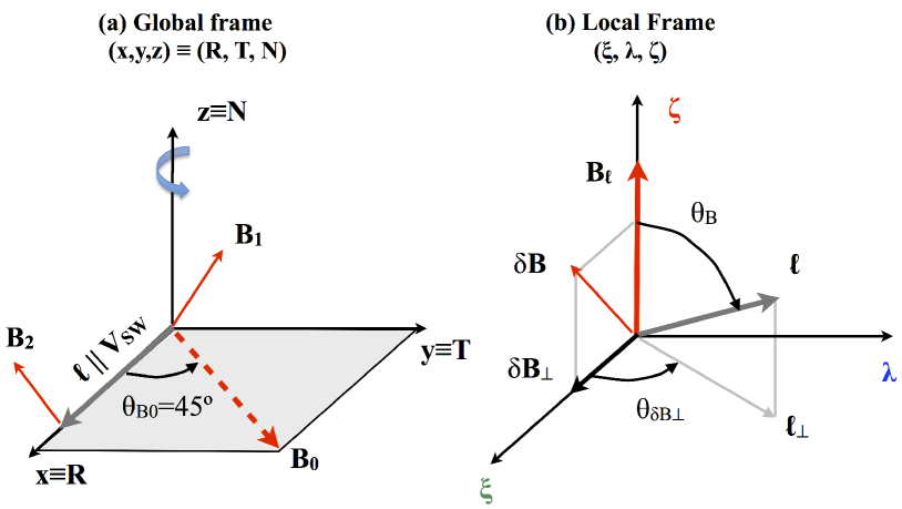
Figure 1.— Panel (a). Reference frame for simulations at $t=t^{*}$. The R, T, N directions correspond to the $x,~{}y,~{}z$ coordinates of the numerical domain. The mean magnetic field ${\boldsymbol{B_{0}}}$ forms an angle $\theta_{B0}=45^{o}$ with the direction of increments ${\boldsymbol{\ell}}=\ell{\boldsymbol{\hat{x}}}$ connecting the fluctuations ${\boldsymbol{B_{1}}}$ and ${\boldsymbol{B_{2}}}$. Panel (b). Local reference frame for computing the 3D anisotropy of structure functions. The axes $\zeta,~{}\xi,~{}\lambda$ and the angles $\theta_{B},~{}\theta_{\delta B\bot}$ are defined for each couple of points by the local magnetic field ${\boldsymbol{B_{\ell}}}=({\boldsymbol{B_{1}}}+{\boldsymbol{B_{2}}})/2$ and by the fluctuation $\delta{\boldsymbol{B}}={\boldsymbol{B_{2}}}-{\boldsymbol{B_{1}}}$.

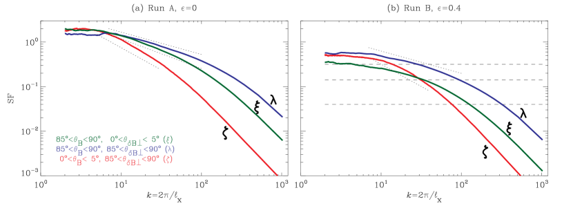
Figure 2.— Second order SF for the non expanding run, panel (a), and expanding run, panel (b) (compare to Figure 1 in Chen et al. 2012), as a function of $k=2\pi/\ell_{x}$. SF are accumulated at three different couples of angles, $\theta_{B}$ and $\theta_{\delta B_{\bot}}$, corresponding to the parallel direction ($\zeta$, red line) and the two perpendicular directions ($\lambda$ in blue, $\xi$ in green) respectively (see Figure 1b). The dotted lines are a reference for the scaling $k^{-1/2},~{}k^{-2/3}$ and $k^{-1}$ in panel (a) and for $k^{-1/2},~{}k^{-1}$ in panel (b). The horizontal dashed lines in panel (b) mark the levels at which isosurfaces are drawn in Figure 3.

To compute the anisotropy of structure functions we use the procedure described in Chen et al. (2012). For each couple of points ${\boldsymbol{x_{1}}},~{}{\boldsymbol{x_{2}}}$ separated by the increment ${\boldsymbol{\ell}}={\boldsymbol{x_{2}}}-{\boldsymbol{x_{1}}}$, we define the local mean field as ${\boldsymbol{B_{\ell}}}=1/2({\boldsymbol{B_{1}}}+{\boldsymbol{B_{2}}})$ and the fluctuating field as $\delta{\boldsymbol{B}}={\boldsymbol{B_{2}}}-{\boldsymbol{B_{1}}}$, where ${\boldsymbol{B_{1,2}}}={\boldsymbol{B}}({\boldsymbol{x_{1,2}}})$. The local scale-dependent reference frame, shown in Figure 1b, has the vertical axis $\zeta$ oriented along ${\boldsymbol{B_{\ell}}}$, the first perpendicular axis $\xi$ oriented along the perpendicular fluctuation direction $\delta{\boldsymbol{B_{\bot}}}\propto{\boldsymbol{B_{\ell}}}\times[\delta{\boldsymbol{B}}\times{\boldsymbol{B_{\ell}}}]$, and the second perpendicular axis $\lambda$ perpendicular to both ${\boldsymbol{B_{\ell}}}$ and $\delta{\boldsymbol{B_{\bot}}}$. In this reference frame, the polar and azimuthal angles $\theta_{B}$ and $\theta_{\delta{\boldsymbol{B}}\bot}$ define the direction of increment with respect to the local mean field. For each pair of points the ${\boldsymbol{B}}$-trace structure function, $\mathrm{SF}=|\delta{\boldsymbol{B}}|^{2}$, is accumulated in $5^{o}$ bins for $\theta_{B},\theta_{\delta{\boldsymbol{B}}\bot}\in[0^{o},90^{o}]$, and then averaged in each bin (we reflected below $90^{o}$ any angles larger than $90^{o}$). Increments, except when otherwise stated, are computed along the $x$ direction ${\boldsymbol{\ell}}={\boldsymbol{\ell_{x}}}$, corresponding to spacecraft flybys along the radial direction in the solar wind frame, as in observations.

We first present the results of the flyby analysis on simulated data at $t^{*}=2.8$ for run A and at $t^{*}=10$ for run B. We then show how the anisotropy evolves in time in the two runs. While $t^{*}$ in run B is chosen to reproduce data at $R=1$ AU, the choice for run A is arbitraty. Homogeneous runs evolve more rapidly than expanding runs since, in the latter, fluctuations are damped by both turbulence and expansion and so the nonlinear time increases more rapidly. We thus chose a different time in run A, after the peak of current density ($t\sim 2.4$) but not too late, in order to have a Reynolds number $Re\approx 1200$ and $B_{rms}/B_{0}\approx 0.9$ comparable to those of run B at $t^{*}=10$ ($B_{rms}/B_{0}\sim 1.5$ and $Re\approx 1300$) .

3. Results

In Figure 2a we plot the SF of the homogenous run A as a function of wavenumber $k=2\pi/\ell_{x}$ for three couples of angle $\theta_{B},~{}\theta_{\delta B\bot}$ corresponding to the directions $\xi,\lambda,\zeta$ in the local reference frame of Figure 1b. Increments are taken along the $x$ direction, which forms an angle of $45^{o}$ with the mean field $B_{0}$. At large scales $k\lesssim 8$ the SFs have comparable energy in the three directions. At small scales, $8\lesssim k\lesssim 60$, we have $\mathrm{SF}(\lambda)>\mathrm{SF}(\xi)>\mathrm{SF}(\zeta)$ with the the following approximate scaling $\mathrm{SF}\propto\lambda^{1/2},~{}\xi^{2/3},~{}\zeta^{1}$ (the power-law range is actually smaller in $\xi$ and $\zeta$).

In panel (b) we show the same plot for the expanding run B. Its overall structure differs completely from run A. Now $\mathrm{SF}(\lambda)$ and $\mathrm{SF}(\xi)$ have parallel profiles roughly proportional to $\lambda^{1/2},~{}\xi^{1/2}$ in the small-scale range, $10\lesssim k\lesssim 50$. $\mathrm{SF}(\lambda)$ is dominant everywhere, while $\mathrm{SF}(\zeta)$ passes from almost dominant at large scales ($k\lesssim 10$) to subdominant at small scales, where the ordering is the same as for the homogeneous run A.

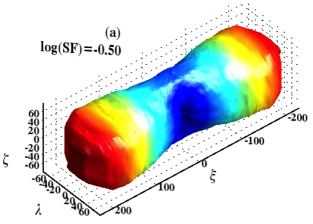
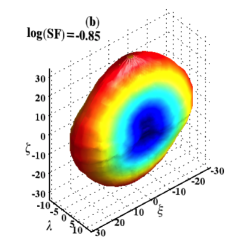
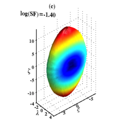
Figure 3.— Run B. Isosurface of constant SF power at three levels, $\textrm{log}\mathrm{SF}=-0.55,~{}-0.85,~{}-1.4$, corresponding to smaller and smaller scales respectively (horizontal dashed lines in Figure 2). Colors indicate distance from the origin to help the 3D visualization. Compare to Figure 4 in Chen et al. (2012).

Following Chen et al. (2012), another viewpoint of the anisotropy in the expanding case is given in Figure 3, where we plot the isosurfaces of constant SF power at three different levels (marked as dashed lines in Figure 2b), corresponding, from left to right, to smaller and smaller scales. For a given value of the isosurface, its shape indicates the correlation of fluctuations along the three directions of the local frame, and can be roughly thought as a statistical eddy shape. Since $\mathrm{SF}=|\delta{\boldsymbol{B}}|^{2}$ measures the power in the anticorrelation, the more energetic is the SF along a given direction, the smaller its correlation. In Figure 3, the smallest correlation (smallest elongation of the isosurface) is always in the $\lambda$ direction, but the direction of the largest correlation changes with scales. At large scales (Figure 3a), the eddy is more elongated in the $\xi$ direction, corresponding to $\delta{\boldsymbol{B_{\bot}}}$, at small scales (Figure 3c) it becomes more elongated along the $\zeta$ direction, corresponding to ${\boldsymbol{B_{\ell}}}$.

The anisotropy shown in Figure 2b and Figure 3 are in very good agreement with the observations of Chen et al. (2012). In Figure 2b the small-scale anisotropy ($10\lesssim k\lesssim 50$) is roughly consistent with critical balance, while the large-scale behavior ($k\lesssim 10$) requires some more explanation.

Figure 4.— (a) Energy spectra at $t^{*}$ along the radial direction $\mathrm{k}_{x}$ for run A (top curves) and run B (bottom curves) for the three R, T, N components of the magnetic field, $B_{x},~{}B_{y},~{}B_{z}$ (dashed, solid, and dotted lines respectively). (b) Evolution with time of the structure function anisotropy $\mathrm{SF}(\zeta)/\mathrm{SF}(\xi)|$ (thick line) computed at $k=2\pi/\ell_{x}=8$ and of the component anisotropy $A=\sqrt{(E_{B}^{y}+E_{B}^{z})/2E_{B}^{x}}$ (thin line) computed at $\mathrm{k}_{x}=8$ for run A (top) and run B (bot). Asterisks indicate the time $t^{*}$ at which the flyby analysis is presented.

The large-scales ordering of SFs is related to the component anisotropy of the magnetic fluctuations that originates from the selective damping induced by the expansion. The component anisotropy is shown in Figure 4a, where we plot the reduced energy spectra $E_{B}^{x,y,z}(\mathrm{k}_{x})$ of the $x,~{}y$, and $z$ components of the magnetic fluctuations compensated by $\mathrm{k}_{x}^{5/3}$, for runs A and B. While in the non-expanding case energy is distributed isotropically among the components, in the expanding case the radial component is at least a factor 2 smaller, at all scales. This behavior is consistent with observations (Horbury & Balogh, 2001) and is generally found in expanding runs (see Dong et al. 2014). The link between the component anisotropy and the SF anisotropy is shown in Figure 4b where we plot their evolution with time. The SF anisotropy is quantified as the ratio $\mathrm{SF}(\zeta)/\mathrm{SF}(\xi)$ at $k=2\pi/\ell_{x}=8$ (see Esquivel & Lazarian 2011; Burkhart et al. 2014 for a similar analysis on global SF), while the component anisotropy is evaluated as $A=\sqrt{(E_{B}^{y}+E_{B}^{z})/2E_{B}^{x}}$ at $\mathrm{k}_{x}=8$. For the homogenous run A, both ratios are about constant and close to the value of 1 (isotropy), while in run B both ratios increase steadily and approximately with the same rate. Thus, in the expanding case as the heliocentric distance increases the magnetic fluctuations are more and more confined in the $y,z$ plane (the T,N plane), and so also the local mean field will preferentially lie in this plane.

We now show that when the SF is sampled along the radial direction, the above component anisotropy, $E_{B}^{y},E_{B}^{z}>E_{B}^{x}$, implies that the SF has a different power along the three directions $\xi,\lambda,\zeta$ defining the local reference frame. Consider two vectors ${\boldsymbol{B_{1}}},~{}{\boldsymbol{B_{2}}}$ at positions $x_{1}$ and $x_{2}$ and indicate with ${\boldsymbol{B^{\bot}_{1,2}}}$ their components in the $y,z$ plane (${\boldsymbol{B^{\bot}}}={\boldsymbol{B_{y}}}+{\boldsymbol{B_{z}}}$), with $\alpha$ the angle between them, and with $B^{\|}_{1,2}$ their projection along $x$. Assume also for simplicity

$$B_{1,2}^{\|}\sim{{\cal O}({2})}<<B^{\bot}_{1}={{\cal O}({1})}=1.$$ (1)

The local mean field and the fluctuation in the $y,z$ plane are given by

$${\boldsymbol{B}}_{\boldsymbol{\ell}}^{\bot}=\sqrt{1+{B^{\bot}_{2}}^{2}+2B^{\bot}_{2}\cos\alpha},$$ (2)

$$\delta{\boldsymbol{B}}^{\bot}=\sqrt{1+{B^{\bot}_{2}}^{2}-2B^{\bot}_{2}\cos\alpha}$$ (3)

($\delta{\boldsymbol{B^{\bot}}}$ should not be confused with $\delta{\boldsymbol{B_{\bot}}}$ that defines the local reference frame). These equations simply state that when ${\boldsymbol{B}}_{1}^{\bot}$ and ${\boldsymbol{B}}_{2}^{\bot}$ are aligned (anti-aligned) the local field $B_{\ell}^{\bot}$ is large (small) and the fluctuating field $\delta B^{\bot}$ is small (large). The orientation of the local reference frame with respect to the fixed radial direction $x$ determines which local SF we are measuring: we cumulate the power in $\mathrm{SF}(\lambda)$ or in $\mathrm{SF}(\zeta)$ or in $\mathrm{SF}(\xi)$ when $\lambda$ or $\zeta$ or $\xi$ lies along $x$. We thus estimate the leading order contributions associated to each of them by considering the power $|\delta{\boldsymbol{B}}|^{2}$ associated to the above three orientations:

• To have power in $\mathrm{SF}(\lambda)$ one needs both ${\boldsymbol{B_{\ell}}}$ and $\delta{\boldsymbol{B}}$ to lie in the $y,z$ plane, that is, $B_{\ell}^{\bot}>>B_{\ell}^{\|}$ and $\delta B^{\bot}>>\delta B^{\|}$. This condition is readily satisfied from Equation (1), provided that $B^{\bot}_{2}<<B^{\bot}_{1}$, or $B^{\bot}_{2}\sim B^{\bot}_{1}$ and $60^{o}\lesssim\alpha\lesssim 120^{o}$ in Equations (2)-(3), yielding in both cases $\mathrm{SF}(\lambda)\sim|\delta{\boldsymbol{B^{\bot}}}|^{2}\sim{{\cal O}({1})}$.

• The contribution to $\mathrm{SF}(\zeta)$ is obtained when ${\boldsymbol{B_{\ell}}}$ is aligned along $x$, that is $B_{\ell}^{\bot}<<B_{\ell}^{\|}$. This happens only when $B^{\bot}_{2}\sim B^{\bot}_{1}$ and $120^{o}<<\alpha\lesssim 180^{o}$ in Equation (2), implying from Equation (3) a contribution $\mathrm{SF}(\zeta)\sim|\delta{\boldsymbol{B^{\bot}}}|^{2}\sim{{\cal O}({1})}$.

• Finally, to have power in $\mathrm{SF}(\xi)$, ${\boldsymbol{B_{\ell}}}$ must belong the $y,z$ plane and $\delta{\boldsymbol{B}}$ must have a non negligible $x$ component $\delta B^{\|}>\delta B^{\bot}/10$ (our minimum angular resolution is $5^{o}$). The conditions $\delta B^{\bot}\sim\delta B^{\|}\sim{{\cal O}({2})}$ and $B_{\ell}^{\|}<<B_{\ell}^{\bot}\sim{{\cal O}({1})}$ are satisfied in Equations (2)-(3) only when $B^{\bot}_{2}\sim B^{\bot}_{1}$ and $\alpha<<60^{o}$, which yield a power $\mathrm{SF}(\xi)\sim|\delta{\boldsymbol{B^{\bot}}}|^{2}\sim|\delta{\boldsymbol{B^{\|}}}|^{2}\sim{{\cal O}({2})}$.

Thus, the geometrical constraint imposed by the component anisotropy induced by expansion, $E_{B}^{y},E_{B}^{z}>E_{B}^{x}$, favors a local anisotropy with $\mathrm{SF}(\lambda)\geq\mathrm{SF}(\zeta)>\mathrm{SF}(\xi)$, as is indeed found at large scales in Figure 2b and in the solar wind observations.

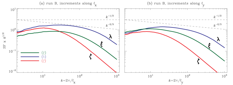
Figure 5.— SF of expanding run B compensated by $k^{1/2}$ as a function of increments computed along the radial directions $k=2\pi/\ell_{x}$ (left), and along the transverse direction $k=2\pi/\ell_{y}$ (right). The two dashed lines are a reference for the scaling $k^{-1/2}$ and $k^{-2/3}$.

We finally show how the anisotropy of expanding turbulence changes if one samples increments in directions perpendicular to the radial. In Figure 5 we plot the SFs of run B computed along $\ell_{x}$ and $\ell_{y}$, corresponding to the R and T directions, respectively. The SFs are now compensated by $k^{1/2}$ to highlight inertial-range scales and the corresponding spectral index. Independently of the direction of increments, the inertial range extends to smaller scales in the second perpendicular direction ($\lambda$) than in the first perpendicular direction ($\xi$). The parallel direction ($\zeta$) does not show any convincing scaling, although having a steeper spectrum. The direction of increments affect the overall anisotropy. In fact, the large-scale ordering, characteristic of expansion in panel (a), disappears when increments are along the transverse direction (panel (b)), the SF becoming basically isotropic for $k\lesssim 10$. This can be interpreted as a reduced effect of the component anisotropy when increments are along the transverse direction (a similar behavior is seen for $\ell=\ell_{z}$, not shown). Moreover the two perpendicular SFs (blue and green curve) exhibit a different spectral index, passing from a slope $\approx 1/2$ in panel (a) to steeper spectral index $\approx 2/3$ in panel (b). Note finally that the eddy shape for transverse increments is at all scales qualitatively similar to the anisotropy in Figure 3c, and thus differs completely from the cases of radial increments shown in Figure 3a,b.

4. Discussion

We computed the 3D anisotropy of structure functions with respect to the local mean field in DNS of MHD turbulence, including or not expansion. For homogenous turbulence, the SF is roughly isotropic at large scales and develops scale-dependent anisotropy at small scales due to the different scaling along the different local directions. The corresponding spectral indices are roughly consistent with $-1/2,~{}-2/3,$ and $-1$ in the $\lambda,~{}\xi$ and $\zeta$ directions respectively. Such an ordering has been predicted by Boldyrev (2006) and implies that $\mathrm{SF}(\lambda)>\mathrm{SF}(\xi)>\mathrm{SF}(\zeta)$ at small scales. The homogenous run qualitatively agrees with the above power anisotropy, which is stable although the precise slopes vary with time and with sampling direction.

When expansion is taken into account the anisotropy is determined by a well-defined large-scale power anisotropy and by a different scaling along the parallel direction ($\zeta$) and the two perpendicular directions ($\lambda,~{}\xi$), the latter now having approximately the same spectral index ($\approx-1/2$). We found that the overall SF anisotropy is a consequence of the component anisotropy induced by expansion and that it shows up only when increments are computed along the radial direction. When increments are along the transverse direction, the large-scale anisotropy disappears, the eddy shape does not change with scales (although the anisotropy increases at smaller and smaller scales), and the SFs exhibit steeper spectral scaling. Thus, the measured anisotropy of solar wind turbulence would change for increments in directions other than the radial, a situation that may become possible to test with Solar Probe Plus in its near-sun orbital phase.

Let us compare our results with the observations in the fast solar wind (Chen et al., 2012). In run B the choice of the solar wind speed yields, via the Taylor hypothesis, the spacecraft frequencies corresponding to the radial increments in Figure 2 and Figure 3. For a fast wind $V_{SW}\sim 800~{}\mathrm{km~{}s^{-1}}$, one gets $f_{min}=V_{SW}R_{x}^{0}/L^{0}\sim 3~{}10^{-5}~{}\mathrm{Hz}$ and $f_{max}=512\times f_{min}\sim 1.5~{}10^{-2}~{}\mathrm{Hz}$. Our initial fluctuations have vanishing $u,B$ correlations for easier comparison between the expanding and homogenous runs, while fast wind has high correlations. Contrary to the non-expanding case, initially highly correlated fluctuations lead to fully developed turbulence in expanding runs (Verdini & Grappin, 2015), with a SF anisotropy similar to (expanding) runs with vanishing $u,B$ correlations. Finally, for scales in between 5-10 hours, the ratio $u_{rms}/V_{SW}\approx 0.1$ for both fast and slow wind (Grappin et al., 1990), thus the expanding parameter $\epsilon=0.4$ is suited for both types of wind. To conclude, as far as the local anisotropy is concerned, the results presented in this Letter are representative of both fast and slow wind and match observations in the fast solar wind, including the change of anisotropy with scales. They indicate that expansion, by distributing energy among different components of the magnetic fluctuations, affects the local mean field orientation and hence the observed anisotropy with respect to it. The present results complement those ones obtained in the recent numerical study by Dong et al. (2014) on the global anisotropy in the solar wind. Both studies show that expansion strongly affects anisotropy of solar wind turbulence at inertial range scales. Finally, the convergence found with observations proves the validity of the EBM approach to model and study solar wind turbulence.

Acknowledgments We thank the referee for useful and constructive comments. This project has received funding from the European Union’s Seventh Framework Programme for research, technological development and demonstration under grant agreement No. 284515 (SHOCK). Website: project-shock.eu/home/. AV acknowledges the Interuniversity Attraction Poles Programme initiated by the Belgian Science Policy Office (IAP P7/08 CHARM). HPC resources were provided by CINECA (grant 2014 HP10CLF0ZB and HP10CNMQX2M).

References

- Beresnyak & Lazarian (2009) Beresnyak, A. & Lazarian, A. 2009, The Astrophysical Journal, 702, 1190
- Bieber et al. (1996) Bieber, J. W., Wanner, W., & Matthaeus, W. H. 1996, J. Geophys. Res., 101, 2511
- Boldyrev (2005) Boldyrev, S. 2005, The Astrophysical Journal, 626, L37
- Boldyrev (2006) —. 2006, Physical Review Letters, 96, 115002
- Bruno & Carbone (2013) Bruno, R. & Carbone, V. 2013, Living Reviews in Solar Physics, 10, 2
- Burkhart et al. (2014) Burkhart, B., Lazarian, A., Leão, I. C., de Medeiros, J. R., & Esquivel, A. 2014, ApJ, 790, 130
- Chen et al. (2012) Chen, C. H. K., Mallet, A., Schekochihin, A. A., Horbury, T. S., Wicks, R. T., & Bale, S. D. 2012, The Astrophysical Journal, 758, 120
- Chen et al. (2011) Chen, C. H. K., Mallet, A., Yousef, T. A., Schekochihin, A. A., & Horbury, T. S. 2011, Monthly Notices of the Royal Astronomical Society, 415, 3219
- Cho & Vishniac (2000) Cho, J. & Vishniac, E. T. 2000, The Astrophysical Journal, 539, 273
- Coleman (1968) Coleman, P. J. J. 1968, Astrophysical Journal, 153, 371
- Dasso et al. (2005) Dasso, S., Milano, L. J., Matthaeus, W. H., & Smith, C. W. 2005, The Astrophysical Journal, 635, L181
- Dong et al. (2014) Dong, Y., Verdini, A., & Grappin, R. 2014, ApJ, 793, 118
- Esquivel & Lazarian (2011) Esquivel, A. & Lazarian, A. 2011, ApJ, 740, 117
- Grappin (1986) Grappin, R. 1986, Physics of Fluids, 29, 2433
- Grappin et al. (1990) Grappin, R., Mangeney, A., & Marsch, E. 1990, JGR, 95, 8197
- Grappin et al. (2013) Grappin, R., Müller, W.-C., Verdini, A., & Gürcan, Ö. 2013, ArXiv e-prints
- Grappin & Velli (1996) Grappin, R. & Velli, M. 1996, J. Geophys. Res., 101, 425
- Grappin et al. (1993) Grappin, R., Velli, M., & Mangeney, A. 1993, Phys. Rev. Lett., 70, 2190
- Hamilton et al. (2008) Hamilton, K., Smith, C. W., Vasquez, B. J., & Leamon, R. J. 2008, J. Geophys. Res., 113, 01106
- He et al. (2013) He, J., Tu, C.-Y., Marsch, E., Bourouaine, S., & Pei, Z. 2013, The Astrophysical Journal, 773, 72
- Horbury & Balogh (2001) Horbury, T. S. & Balogh, A. 2001, J. Geophys. Res., 106, 15929
- Horbury et al. (2008) Horbury, T. S., Forman, M., & Oughton, S. 2008, Physical Review Letters, 101, 175005
- Luo & Wu (2010) Luo, Q. Y. & Wu, D. J. 2010, The Astrophysical Journal Letters, 714, L138
- Matthaeus et al. (1990) Matthaeus, W. H., Goldstein, M. L., & Roberts, D. A. 1990, Journal of Geophysical Research (ISSN 0148-0227), 95, 20673
- Milano et al. (2001) Milano, L. J., Matthaeus, W. H., Dmitruk, P., & Montgomery, D. C. 2001, Physics of Plasmas, 8, 2673
- Montgomery & Turner (1981) Montgomery, D. & Turner, L. 1981, Physics of Fluids, 24, 825
- Narita et al. (2010) Narita, Y., Glassmeier, K.-H., Sahraoui, F., & Goldstein, M. L. 2010, Physical Review Letters, 104, 171101
- Podesta (2009) Podesta, J. J. 2009, The Astrophysical Journal, 698, 986
- Saur & Bieber (1999) Saur, J. & Bieber, J. W. 1999, Journal of Geophysical Research, 104, 9975
- Shebalin et al. (1983) Shebalin, J. V., Matthaeus, W. H., & Montgomery, D. 1983, Journal of Plasma Physics, 29, 525
- Verdini & Grappin (2015) Verdini, A. & Grappin, R. 2015, in preparation
- Verdini et al. (2015) Verdini, A., Grappin, R., Hellinger, P., Landi, S., & Müller, W. C. 2015, The Astrophysical Journal, 804, 119
- Wicks et al. (2012) Wicks, R. T., Forsyth, M. A., Horbury, T. S., & Oughton, S. 2012, The Astrophysical Journal, 746, 103
- Wicks et al. (2010) Wicks, R. T., Horbury, T. S., Chen, C. H. K., & Schekochihin, A. A. 2010, Monthly Notices of the Royal Astronomical Society: Letters, 407, L31, (c) Journal compilation © 2010 RAS
- Wicks et al. (2011) —. 2011, Physical Review Letters, 106, 45001
- Wicks et al. (2013) Wicks, R. T., Roberts, D. A., Mallet, A., Schekochihin, A. A., Horbury, T. S., & Chen, C. H. K. 2013, The Astrophysical Journal, 778, 177