Higher-dimensional thin-shell wormholes in third-order Lovelock gravity

Abstract

In this work, we explore asymptotically flat charged thin-shell wormholes of third order Lovelock gravity in higher dimensions, taking into account the cut-and-paste technique. Using the generalized junction conditions, we determine the energy-momentum tensor of these solutions on the shell, and explore the issue of the energy conditions and the amount of normal matter that supports these thin-shell wormholes. Our analysis shows that for negative second order and positive third-order Lovelock coefficients, there are thin-shell wormhole solutions that respect the weak energy condition. In this case, the amount of normal matter increases as the third-order Lovelock coefficient decreases. We also find novel solutions which possess specific regions where the energy conditions are satisfied for the case of a positive second order and negative third-order Lovelock coefficients. Finally, a linear stability analysis in higher dimensions around the static solutions is carried out. Considering a specific cold equation of state, we find a wide range of stability regions.

I INTRODUCTION

Wormholes are topologically nontrivial objects which connect two separate and distinct spacetime regions MT ; MTY . A fundamental ingredient in wormhole physics is the flaring-out condition of the throat, which in General Relativity (GR) entails the violation of the null energy condition (NEC). Matter that violates the NEC is denoted exotic matter. In fact, wormholes violate all of the pointwise and averaged energy condition MTY . Due to the problematic nature of these violations, it is useful to minimize the exoticity problem of the matter threading and sustaining the wormhole. For instance, traversable wormholes supported by arbitrarily small quantities of exotic matter viskardad or by matter respecting the energy conditions MartRich ; Deh1 ; wecsat ; Harko:2013yb have been investigated.

An interesting kind of traversable wormhole is the thin-shell variety constructed by surgically grafting together two spacetimes to form a geodesically complete manifold with a shell placed at the junction interface. In these types of wormholes, matter is concentrated on the wormhole throat, which coincides with the junction boundary, and thus minimizes the usage of exotic matter. These solutions were initially presented in Vis ; VisP and have been extensively investigated in the literature thin ; lemo11 . In GR, it was shown that thin-shell wormholes inevitably violate the weak energy condition (WEC) and, consequently, various attempts have been undertaken, to alleviate this problem, in alternative theories of gravity, for instance, in dilatonic gravity bej , Brans-Dicke theory yueca and DGP gravity cyl . An advantage of the thin-shell construction is that one may consider a linearized stability analysis around the static solution, while preserving the symmetric configuration, and analyse the dynamical evolution of the thin-shell brad . The generalization of the stability analysis to the case of higher-dimensional wormholes has also been extensively investigated rah1 . For instance, a linearized stability analysis in the presence of a dilaton, axion, phantom and other types of matter and in cylindrical symmetry have also been studied eir .

Since string theory proposes higher dimensional gravitational objects, it is of interest to explore the possibility of higher dimensional thin-shell wormhole solutions. One of the most interesting higher dimensional alternative theories of gravity which leads to second order field equations for the metric is described by the Lovelock action lovee . In this context, thin shell wormholes of second order Lovelock theory called Gauss-Bonnet theory in $5$-dimensions and higher dimensions were extensively analysed mazv . In the context of third order Lovelock gravity, asymptotically flat and charged thin-shell wormholes of Lovelock gravity in seven dimensions were constructed, using the cut-and-paste technique, and the generalized junction conditions were applied in order to calculate the energy-momentum tensor of these wormholes on the shell meh . It was found that for negative second order and positive third order Lovelock coefficients, there are thin-shell wormholes that respect the WEC in specific regions. In this case, the amount of normal matter decreases as the third order Lovelock coefficient increases. For positive second and third order Lovelock coefficients, the WEC is violated and the amount of exotic matter decreases as the charge increases. Furthermore, a linear stability analysis was analysed against a symmetry preserving perturbation, and the stability of these wormhole were studied.

In this work, we extend the analysis outlined in meh , by providing the explicit form of the surface energy-momentum tensor and generalize the analysis to arbitrary dimensions. More specifically, we present the explicit form of the energy-momentum tensor in terms of the extrinsic curvature and Riemann tensor for all higher dimensions, and find specific solutions, including novel solutions which possess specific regions where the energy conditions are satisfied for the particular cases of positive second order and negative third-order Lovelock coefficients. Furthermore, we present the generalized junction conditions, and analyse the stability analysis for the solutions found, for arbitrary dimensions. Thus, we study the effects of the third order Lovelock term in higher dimensionality, its role in the satisfaction of the WEC and the stability of thin shell wormhole solutions in higher dimensions.

This paper is organised in the following manner: In Section II, we present the action of third order Lovelock gravity in the presence of an electromagnetic field, and construct a thin-shell wormhole in Lovelock gravity, by presenting explicitly the surface energy-momentum tensor components on the shell. In particular, to complement the above Section II, the specific $(n+1)$-dimensional static solutions, that are to be used throughout the work, are outlined in Appendix A. In Appendix B, we also introduce the junction conditions in Lovelock gravity, in order to construct the thin-shell wormhole. In Section III, we analyse the profile of the surface stresses and consider the issue of the energy conditions and the amount of normal matter supporting the thin-shell wormhole. In Section IV, we study the stability of the thin-shell wormholes under small perturbations preserving the symmetry of the wormhole configuration, and explore the dynamical evolution of the shell. Finally, in Section V, we conclude.

II ACTION AND THIN-SHELL CONSTRUCTION

The action of third order Lovelock gravity in the presence of an electromagnetic field may be written as

$$I=\int d^{n+1}x\sqrt{-g}\left(\mathcal{L}_{1}+\alpha_{2}\mathcal{L}_{2}+\alpha_{3}\mathcal{L}_{3}-F_{\mu\nu}F^{\mu\nu}\right)\,,$$ (1)

where $\alpha_{2}$ and $\alpha_{3}$ are the second (Gauss-Bonnet) and third order Lovelock coefficients. The term $\mathcal{L}_{1}=R$ is the Einstein-Hilbert Lagrangian, $\mathcal{L}_{2}$ is the Gauss-Bonnet Lagrangian, and $\mathcal{L}_{3}$ is the third order Lovelock Lagrangian, which are defined in Appendix A.

The electromagnetic tensor is defined as $F_{\mu\nu}=\partial_{\mu}A_{\nu}-\partial_{\nu}A_{\mu}$, where the vector potential $A_{\mu}$ is given by

$$A_{\mu}=\sqrt{\frac{(n-1)}{2(n-2)}}\frac{q}{r^{n-2}}\delta_{\mu}^{t}.$$ (2)

The $(n+1)$-dimensional static solution of action (1) is given in the form

$$ds^{2}=-f(r)dt^{2}+\frac{dr^{2}}{f(r)}+r^{2}d\Sigma_{n-1}^{2},$$ (3)

where $d\Sigma_{n-1}^{2}$ is the metric of a $(n-1)$-dimensional unit sphere and the metric function $f(r)$ is given by

$$f(r)=1-r^{2}\psi(r),$$ (4)

where the solutions for the function $\psi(r)$ are outlined in the Appendix A.

To construct a thin-shell wormhole in third order Lovelock gravity, we use the well-known cut-and-paste technique. The junction conditions in Lovelock gravity are given in Appendix B, where we refer the reader for more details. Taking two copies of the asymptotically flat solutions of Lovelock gravity given by Eqs. (3) and (4) and solutions of Eq. (28) and removing from each manifold the $(n+1)$-dimensional region described by

$$\Omega_{\pm}=\left\{r_{\pm}\leq a,a>r_{h}\right\},$$ (5)

we are left with two geodesically incomplete manifolds with the following timelike hypersurface as boundaries

$$\Sigma_{\pm}=\left\{r_{\pm}=a,a>r_{h}\right\}.$$ (6)

Now identifying these two boundaries, $\Sigma_{+}=\Sigma_{-}=\Sigma$, we obtain a geodesically complete manifold containing the two asymptotically flat regions $\Omega_{+}$ and $\Omega_{-}$ which are connected by a wormhole. The throat of the wormhole is located at $\Sigma$ with the following metric

$$ds_{\Sigma}^{2}=-d\tau^{2}+a^{2}(\tau)d\Omega_{n-1}^{2},$$ (7)

where $\tau$ is the proper time along the hypersurface $\Sigma$ and $a(\tau)$ is the radius of the throat. In order to study the stability of the thin-shell wormhole constructions, we allow the radius of the throat to be a function of the proper time. In addition to this, note that all the matter is concentrated on the wormhole throat, $\Sigma$.

To analyze such a thin-shell configuration, we need to use the modified junction conditions. Considering the induced coordinates on $\Sigma$, $\xi^{a}=(\tau,\theta^{i};$ $i=1...n)$, the extrinsic curvatures associated with the two sides of the shell are given by

$${\mathcal{K}}_{ab}^{\pm}=-n_{\rho}^{\pm}\left(\frac{\partial^{2}X^{\rho}}{\partial\xi^{a}\partial\xi^{b}}+\Gamma_{\mu\nu}^{\rho}\frac{\partial X^{\mu}}{\partial\xi^{a}}\frac{\partial X^{\nu}}{\partial\xi^{b}}\right)_{r=a},$$ (8)

where the normal vector $n_{\rho}^{\pm}$ ($n_{\rho}n^{\rho}=1$) to the surface $\Sigma$ in $\mathcal{M}$ is defined by

$$n_{\gamma}^{\pm}=\pm\left|g^{\mu\nu}\frac{\partial\mathcal{G}}{\partial X^{\mu}}\frac{\partial\mathcal{G}}{\partial X^{\nu}}\right|\frac{\partial\mathcal{G}}{\partial X^{\gamma}}\,,$$ (9)

where $\mathcal{G}(r,\tau)$ is the equation of the boundary $\Sigma$, given by

$$\mathcal{G}(r,\tau)=r-a(\tau)=0.$$ (10)

After some algebraic manipulations, in an orthonormal basis $\{e_{\hat{\tau}},e_{\hat{\imath}};$ $i=1...n-1\}$, the components of the extrinsic curvature tensor are given by

$$\mathcal{K}_{~{}\hat{\tau}}^{\hat{\tau}} = \frac{\Gamma}{\Delta},$$ (11)

$$\mathcal{K}_{\hat{\jmath}}^{\hat{\imath}} = \frac{\Delta}{a}~{}\delta_{\hat{\jmath}}^{\hat{\imath}}$$ (12)

with

$$\Gamma=\ddot{a}+\frac{f^{\prime}\left(a\right)}{2},\qquad\Delta=\sqrt{\dot{a}^{2}+f\left(a\right)},$$

where the prime and the overdot denote derivatives with respect to $a$ and $\tau$, respectively. Equations (11) and (12) show that the form of the energy-momentum tensor on the shell is ${S}_{~{}\hat{b}}^{\hat{a}}=~{}\mbox{diag}~{}(-\sigma,p~{}\delta_{\hat{\jmath}}^{\hat{\imath}})$, where $\sigma$ is the surface energy density and $p$ is the transverse pressure.

Now using the junction condition (39), the components of the energy-momentum tensor on the shell may be written as

$$\sigma = -S_{\tau}^{\tau}=-\frac{\Delta}{4\pi}\bigg{\{}\frac{(n-1)}{a}-\frac{2\tilde{\alpha}_{2}(n-1)}{3a^{3}}$$ (13)

$$\times\left[\Delta^{2}-3(1+\dot{a}^{2})\right]+\frac{(n-1)\tilde{\alpha}_{3}}{5a^{5}}$$

$$\times\left[15(1+\dot{a}^{2})^{2}-10\Delta^{2}(1+\dot{a}^{2})+3\Delta^{4}\right]\bigg{\}},$$

$$p = S_{i}^{i}=\frac{1}{8\pi}\bigg{\{}\frac{2\Gamma}{\Delta}+\frac{2(n-2)\Delta}{a}$$ (14)

$$-\frac{4\tilde{\alpha}_{2}}{3a^{2}}\Big{\{}3\Gamma\Delta-\frac{3\Gamma}{\Delta}\left(1+\dot{a}^{2}\right)+\frac{\Delta^{3}(n-4)}{a}$$

$$-\frac{6\Delta}{a}\left[\frac{(n-4)}{2}\left(1+\dot{a}^{2}\right)+\ddot{a}a\right]\Bigg{\}}+\frac{2\tilde{\alpha}_{3}}{5a^{4}}$$

$$\times\Bigg{\{}\frac{15\Gamma}{\Delta}\left(1+\dot{a}^{2}-\Delta^{2}\right)^{2}+20\ddot{a}\Delta\left[3\left(1+\dot{a}\right)-\Delta^{2}\right]$$

$$+\frac{(n-6)\Delta}{5a}[15(1+{\dot{a}}^{2}-\Delta^{2})^{2}$$

$$+20\left(1+\dot{a}^{2}\right)\left(3(1+\dot{a}^{2})-\Delta^{2}\right)]\big{\}}\Big{\}}\,,$$

respectively. From the above equations we see that $\sigma$ and $p$ are expressed in terms of the throat radius $a(\tau)$, the first and second derivatives of $a(\tau)$ and the metric function $f(a)$. Note that the surface energy density and transverse pressure satisfy the energy conservation equation, given by

$$\frac{d}{d\tau}\left(\sigma a^{(n-1)}\right)+p\frac{d}{d\tau}\left(a^{(n-1)}\right)=0.$$ (15)

The first term in Eq. (15) represents the internal energy change of the shell and the second term shows the work by internal forces of the shell.

III PROFILE OF THE SURFACE ENERGY-MOMENTUM ON THE THIN-SHELL

In this section, we consider the issue of the energy conditions and the amount of normal matter that supports the thin-shell wormhole. The WEC is defined as $T_{\mu\nu}V^{\mu}V^{\nu}\geq 0$ for every nonspacelike vector $V_{\mu}$. The WEC on the thin shell is satisfied provided that $\sigma\geq 0$, $\sigma+p\geq 0$. We restrict our analysis to static configurations with $a=a_{0}$ and $\dot{a}=\ddot{a}=0$. For the static configuration, Eqs. (13) and (14) reduce to

$$\sigma_{0} = -\frac{(n-1)}{8\pi a_{0}\sqrt{f_{0}}}\left\{2f_{0}+\frac{4\tilde{\alpha}_{2}}{3a_{0}^{2}}f_{0}(3-f_{0})\right.$$ (16)

$$\left.+\frac{2\tilde{\alpha}_{3}}{5a_{0}^{4}}f_{0}(15-10f_{0}+3f_{0}{}^{2})\right\},$$

$$\sigma_{0}+p_{0} = \frac{1}{8\pi a_{0}\sqrt{f_{0}}}\Big{\{}(-2f_{0}+a_{0}f_{0}^{\prime})$$ (17)

$$+\frac{2\tilde{\alpha}_{2}}{3a_{0}^{2}}\left[3a_{0}f_{0}^{\prime}(1-f_{0})-6f_{0}(3-f_{0})\right]$$

$$+\frac{\tilde{\alpha}_{3}}{a_{0}^{4}}[3a_{0}f_{0}^{\prime}(1-2f_{0}+f_{0}^{2})$$

$$-2f_{0}(15-10f_{0}+3f_{0}{}^{2})]\Big{\}},$$

respectively, where $f_{0}=f(a_{0})$ and $f_{0}^{\prime}=f^{\prime}(a_{0})$. In contrast to the case of general relativistic thin-shell wormholes for which $\sigma_{0}<0$, thus violating the WEC rah1 , in higher-dimensional thin-shell wormholes one can have, in principle, normal matter on the shell. In order to investigate the profile of the surface energy-momentum on the thin-shell, we find the amount of matter on the shell, which is given by

$$\digamma=\int drd\Omega_{n-1}[\sigma_{0}\delta(r-a_{0})+p_{r}].$$ (18)

For our case, the shell does not exert radial pressure, i.e., $p_{r}=0$, and therefore the amount of matter on the shell is

$$\digamma = \frac{2\pi^{\frac{n}{2}}a_{0}^{n-1}\sigma_{0}}{\Gamma(\frac{n}{2})}$$ (19)

$$= \frac{4\pi^{\frac{n}{2}}(n-1)}{\Gamma(\frac{n}{2})}\sqrt{f_{0}}\;\bigg{[}-a_{0}^{(n-2)}+\frac{2\tilde{\alpha}_{2}a_{0}^{(n-4)}}{3}(f_{0}-3)$$

$$+\frac{\tilde{\alpha}_{3}a_{0}^{(n-6)}}{5}\left(-15+10f_{0}-3f_{0}{}^{2}\right)\bigg{]},$$

where $f_{0}$ is the value of $f(r)$ at $r=a_{0}$. In Einstein gravity, $\tilde{\alpha}_{2}=\tilde{\alpha}_{3}=0$, the matter is exotic both for Reissner-Nordstrom $(Q\neq 0)$ and Schwarzschild $(Q=0)$ thin-shell wormholes as one can see from Eq. (19) as $\sigma_{0}<0$ (Eq. (16)). In Gauss-Bonnet gravity, $\alpha_{3}=0$ with $\alpha_{2}\leq 0$, one may have thin-shell wormholes supported by normal matter mazv .

Now, we investigate the condition that thin-shell wormholes may be supported by normal matter in third order Lovelock gravity. It is clear from Eq. (19) that the sign of $\digamma$ depends on the sign of $\sigma_{0}$.

III.1 Specific case: $\tilde{\alpha}_{2}^{2}=3\tilde{\alpha}_{3}=\alpha^{2}$

For the special case $\tilde{\alpha}_{2}^{2}=3\tilde{\alpha}_{3}=\alpha^{2}$, Eq. (16) takes the form

$$\sigma_{0} = -\frac{(n-1)}{60\pi a_{0}^{5}}\big{[}3\alpha^{2}f_{0}^{2}-10\alpha(\alpha+a_{0}^{2})f_{0}$$ (20)

$$+15(\alpha^{2}+2\alpha a_{0}^{2}+a_{0}^{4})\big{]}.$$

The sign of the square brackets in the above equation determines the sign of $\sigma_{0}$. This is a quadratic equation for the metric function $f_{0}$ and one can easily obtain the discriminant of the quadratic equation which is equal to $-80\alpha^{2}(\alpha+a_{0}^{2})^{2}$. Since the discriminant is negative for all values of $\alpha$, the sign of the brackets is always positive and therefore $\sigma_{0}<0$. In other words, the matter supporting the thin-shell wormhole is exotic for any dimensions.

III.2 Specific case: $\alpha_{2}>0$ and $\alpha_{3}>0$

For the general solutions of third order Lovelock gravity we first consider the case where $\tilde{\alpha}_{2}$ and $\tilde{\alpha}_{3}$ are positive. In this case, since the metric function is asymptotically flat ($0<f_{0}<1$) for $a\geqslant r_{h}$, and therefore the factors $3-f_{0}$ and $15-10f_{0}+3f_{0}^{2}$ are positive, the bracket in Eq. (16) is always positive. Therefore, the matter on the throat is exotic in the case of $\tilde{\alpha}_{2},\tilde{\alpha}_{3}>0$ as in this case we have $\sigma_{0}<0$ (or $\digamma<0$ ).

III.3 Specific case: $\alpha_{2}<0$ and $\alpha_{3}>0$

For $\alpha_{3}>0$ and $\alpha_{2}<0$, $\digamma$ can be positive and therefore the matter is normal. For this case, Figs. 1 and 2 display the behaviour of $\sigma_{0}$ and $\sigma_{0}+p_{0}$ for $n=8$ and $9$ respectively. In these plots, there exist regions for $\sigma_{0}\geq 0$ (or $\digamma\geq 0$) and $\sigma_{0}+p_{0}\geq 0$ and therefore the WEC and NEC are satisfied in this region. Since $0<f_{0}<1$, the factor $-15+10f_{0}-3f_{0}^{2}$ in Eq. (19) is negative and therefore the amount of normal matter for negative $\alpha_{2}$ decreases as $\alpha_{3}>0$ increases, as one can see in Figs. 1-a) and 1-b) for $\alpha_{3}=2$ and $\alpha_{3}=1$. In Figs. 2-a) and 2-b), we show that the amount of normal matter increases as $\alpha_{2}<0$ decreases. Also, in this case the amount of normal matter decreases as the charge $q$ increases (see Fig. 3).

III.4 Specific case: $\alpha_{2}>0$ and $\alpha_{3}<0$

Finally, we can see that for $\alpha_{2}>0$ and $\alpha_{3}<0$, $\digamma$ can be positive and therefore, for the first time, we have found thin-shell wormholes threaded by normal matter on the shell in specific regions. In this case, as depicted in Fig. 4, there exist regions for $\sigma_{0}\geq 0$ (or $\digamma\geq 0$) and $\sigma_{0}+p_{0}\geq 0$ and therefore the WEC and NEC are satisfied.

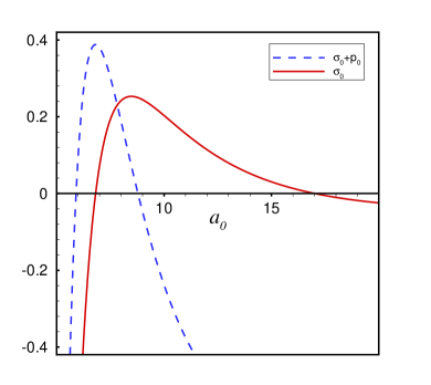
(a)  $\alpha_{3}=2$

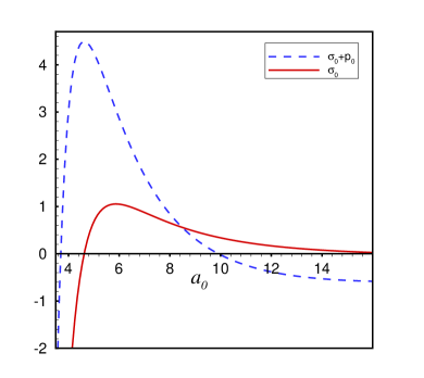
(b)  $\alpha_{3}=1$

Figure 1: Specific case: $\alpha_{2}<0$ and $\alpha_{3}>0$. $\sigma_{0}$ (continuous) and $\sigma_{0}+p_{0}$ (dashed) versus $a_{0}$ for $\alpha_{2}=-2$, $m=100$, $q=3000$ and $n=9$. These figures depict that for $\alpha_{2}<0$ and $\alpha_{3}>0$, the WEC can be satisfied. The plots also show that normal matter for $\alpha_{2}<0$ decreases as $\alpha_{3}>0$ increases.

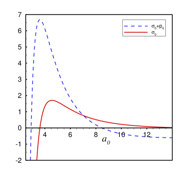
(a) $\alpha_{2}=-2$

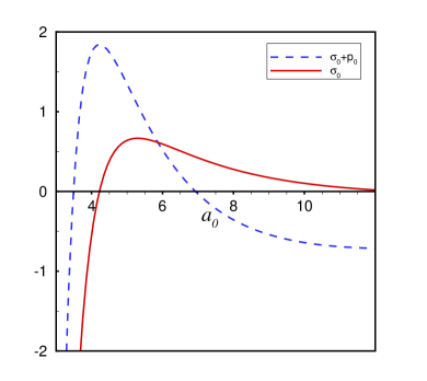
(b)  $\alpha_{2}=-1.5$

Figure 2: Specific case: $\alpha_{2}<0$ and $\alpha_{3}>0$. $\sigma_{0}$ (continuous) and $\sigma_{0}+p_{0}$ (dashed) versus $a_{0}$ for $\alpha_{3}=1$, $m=100$, $q=3000$ and $n=8$. These figures depict that for $\alpha_{2}<0$ and $\alpha_{3}>0$, the WEC can be satisfied. The plots also show that for $\alpha_{3}>0$, the amount of normal matter increases as $\alpha_{2}<0$ decreases.

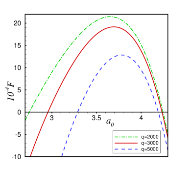
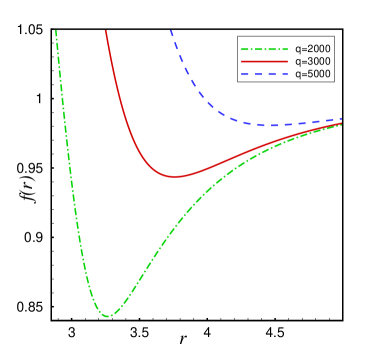
Figure 3: Right: $f(r)$ versus $r$ for $\alpha_{2}=-0.6$, $\alpha_{3}=0.2$, $n=8$, $m=300$ and $q=2000$, $3000$, $5000$ from down to up respectively. Left: $10^{-4}\digamma$ versus $a_{0}$ for $f(r)$ plotted in the right figure. These figures depict that for $\alpha_{3}>0$ and $\alpha_{2}<0$, the amount of normal matter decreases as $q$ increases.

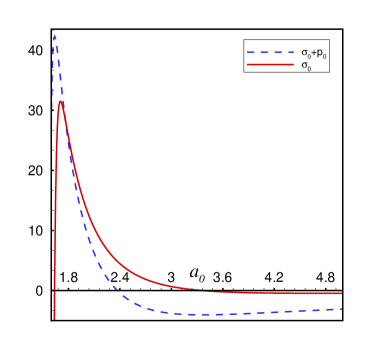
Figure 4: Specific case: $\alpha_{2}>0$ and $\alpha_{3}<0$. $\sigma_{0}$ (continuous) and $\sigma_{0}+p_{0}$ (dashed) versus $a_{0}$ for $\alpha_{2}=0.12$, $\alpha_{3}=-0.1$, $m=10$, $q=1.4$ and $n=8$.

IV STABILITY ANALYSIS

In this section, we study the stability of the thin shell under small perturbations preserving the symmetry of the wormhole configuration. The dynamical evolution of the shell results from Eqs. (13) and (14) or by any of them and the conservation equation (15). In order to analyze the stability and to complete the system we use a cold equation of state $p=p(\sigma)$ with $\eta=dp/d\sigma$. We consider small radial perturbations around a static solution with radius $a_{0}$ and obtain the equation of motion near the equilibrium solution. In this case, one may write $p\simeq p_{0}+\eta_{0}(\sigma-\sigma_{0})$, where $p_{0}$, $\sigma_{0}$ and $\eta_{0}$ are the transverse pressure, surface energy density and $dp/d\sigma$ at the static solution $a=a_{0}$, respectively. Using this linear equation of state, then Eq. (15) yields the following solution for the surface energy energy

$$\sigma\left(a\right)=\left(\frac{\sigma_{0+}p_{0}}{1+\eta}\right)\left(\frac{a_{0}}{a}\right)^{(n-1)\left(1+\eta\right)}+\frac{\eta\sigma_{0-}p_{0}}{1+\eta}\,.$$ (21)

Substituting the energy density (21) in Eq. (14), leads us to the equation of motion, for the radius of the throat, given by

$$-\frac{60\pi a^{5}\sigma(a)}{(n-1)\sqrt{\dot{a}^{2}+f(a)}}=$$

$$3\tilde{\alpha}_{3}\left\{8(1+\dot{a}^{2})^{2}+4[1-f(a)](1+\dot{a}^{2})+3[1-f(a)]^{2}\right\}$$

$$+15a^{4}+10\tilde{\alpha}_{2}a^{2}\left[2(1+\dot{a}^{2})+1-{f(a)}\right],$$ (22)

where $\sigma(a)$ is given in Eq. (21).

The dynamics of the wormhole throat is determined by a single equation with the form of $\dot{a}^{2}=-V(a)$. However, in third order Lovelock gravity, one encounters a fifth order algebraic equation for $\dot{a}^{2}$ and unfortunately one cannot obtain an exact result, but, one may perform the linearized stability analysis numerically. More specifically, one may solve Eq. (22) for $\dot{a}^{2}$ numerically and obtain the potential $V(a)$ in the equation of motion. Then, the wormhole with radius $a_{0}$ is linearly stable provided the potential $V(a)$ is minimum at $a=a_{0}$ where $a(\tau)$ will oscillate about $a_{0}$ and stabilize the wormhole. Numerical calculations are shown in Figs. 5-7 for $n=8$ and $n=9$. In the analysis, we have chosen the regions $a_{0}$ for which matter is normal. As depicted by the figures, for the specific parameter ranges, the wormholes are stable for negative values for $\eta$ and unstable for positive $\eta=dp/d\sigma$. We emphasize that these results are in agreement with those presented in meh , where it was shown through numerical calculations that wormholes are stable provided the parameter $\eta$ is negative and the throat radius $a_{0}$ is adequately chosen.

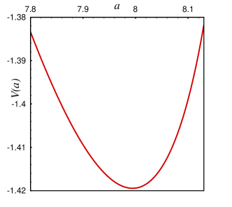
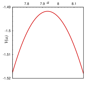
Figure 5: $V(a)$ versus $a$ with $\alpha_{2}=-2$, $\alpha_{3}=2$, $m=100$, $n=9$ and $q=3000$ for $\eta=-3$ (left) and $\eta=3$ (right). These figures depict that wormholes are stable for $\eta=dp/d\sigma<0$ and unstable for $\eta>0$.

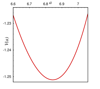
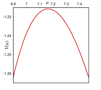
Figure 6: $V(a)$ versus $a$ with $\alpha_{2}=-2$, $\alpha_{3}=1$, $m=300$, $n=8$ and $q=3000$ for $\eta=-2$ (left) and $\eta=1$ (right). These figures depict that wormholes are stable for $\eta=dp/d\sigma<0$ and unstable for $\eta>0$.

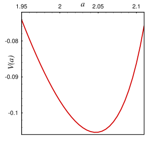
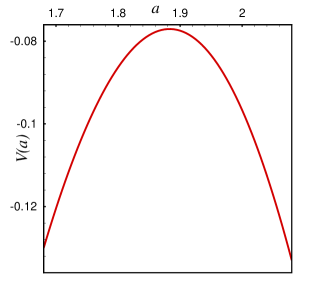
Figure 7: $V(a)$ versus $a$ with $\alpha_{2}=0.12$, $\alpha_{3}=-0.1$, $m=10$, $n=8$ and $q=1.4$ for $\eta=-1.5$ (left) and $\eta=1.5$ (right). These figures depict that wormholes are stable for $\eta=dp/d\sigma<0$ and unstable for $\eta>0$.

V SUMMARY AND DISCUSSION

Motivated by the fact that string theory proposes higher dimensional gravitational objects, we have considered higher-dimensional thin-shell wormholes in the context of third order Lovelock gravity. More specifically, asymptotically flat charged thin-shell wormholes of third order Lovelock gravity in higher dimensions were constructed, taking into account the cut-and-paste technique. We extended the analysis outlined in meh , by providing the explicit form of the surface energy-momentum tensor in terms of the extrinsic curvature and Riemann tensor for all higher dimensions, explored the issue of the energy conditions and the amount of normal matter that supports these thin-shell wormholes. Our analysis shows that for negative second order and positive third-order Lovelock coefficients, there are thin-shell wormhole solutions that respect the weak energy condition. In this case, the amount of normal matter increases as the third-order Lovelock coefficient decreases. We also found novel solutions which possess specific regions where the energy conditions are satisfied for the case of a positive second order and negative third-order Lovelock coefficients. Furthermore, we presented the generalized junction conditions, and analysed the stability analysis for the solutions found, in arbitrary dimensions. This enabled us to study the effects of the third order Lovelock term in higher dimensionality and the satisfaction of the WEC and stability of thin shell wormhole solutions. In the latter context, a linear stability analysis in higher dimensions around the static solutions was carried out, by considering a specific cold equation of state, and a wide range of stability regions were found.

Appendix A Action and spherically symmetric solutions

We reproduce the action of third order Lovelock gravity, in the presence of an electromagnetic field, here

$$I=\int d^{n+1}x\sqrt{-g}\left(\mathcal{L}_{1}+\alpha_{2}\mathcal{L}_{2}+\alpha_{3}\mathcal{L}_{3}-F_{\mu\nu}F^{\mu\nu}\right)\,,$$ (23)

where, as mentioned in Sec. II, $\alpha_{2}$ and $\alpha_{3}$ are the second (Gauss-Bonnet) and third order Lovelock coefficients. The term $\mathcal{L}_{1}=R$ is the Einstein-Hilbert Lagrangian, $\mathcal{L}_{2}$ is the Gauss-Bonnet Lagrangian given by

$$\mathcal{L}_{2}=R_{\mu\nu\gamma\delta}R^{\mu\nu\gamma\delta}-4R_{\mu\nu}R^{\mu\nu}+R^{2}\,,$$ (24)

and the third order Lovelock Lagrangian is defined as

$$\mathcal{L}_{3} = 2R^{\mu\nu\sigma\kappa}R_{\sigma\kappa\rho\tau}R_{\phantom{\rho\tau}{\mu\nu}}^{\rho\tau}+8R_{\phantom{\mu\nu}{\sigma\rho}}^{\mu\nu}R_{\phantom{\sigma\kappa}{\nu\tau}}^{\sigma\kappa}R_{\phantom{\rho\tau}{\mu\kappa}}^{\rho\tau}$$ (25)

$$+24R^{\mu\nu\sigma\kappa}R_{\sigma\kappa\nu\rho}R_{\phantom{\rho}{\mu}}^{\rho}+3RR^{\mu\nu\sigma\kappa}R_{\sigma\kappa\mu\nu}$$

$$+24R^{\mu\nu\sigma\kappa}R_{\sigma\mu}R_{\kappa\nu}+16R^{\mu\nu}R_{\nu\sigma}R_{\phantom{\sigma}{\mu}}^{\sigma}$$

$$-12RR^{\mu\nu}R_{\mu\nu}+R^{3}.$$

In Lovelock gravity only terms with order less than $[(n+1)/2]$ (where $[x]$ is the integer part of $x$) contribute to the field equations, the rest being total derivatives in the action. Therefore one should consider $n\geq 6$ in the case of third order Lovelock gravity so that the effects of third order Lovelock gravity appear.

The $(n+1)$-dimensional static solution of action (23) is given in the form, which we rewrite for self-completeness,

$$ds^{2}=-f(r)dt^{2}+\frac{dr^{2}}{f(r)}+r^{2}d\Sigma_{n-1}^{2},$$ (26)

where $d\Sigma_{n-1}^{2}$ is the metric of a $(n-1)$-dimensional unit sphere and the metric function $f(r)$ is given by

$$f(r)=1-r^{2}\psi(r).$$ (27)

Substituting the electromagnetic potential (2) and the metric (26) into the action (23) and varying the latter with respect to the metric function $f(r)$, one obtains the equation of motion as amira

$$\tilde{\alpha}_{3}\psi^{3}(r)+\tilde{\alpha}_{2}\psi^{2}(r)+\psi(r)-\frac{m}{r^{n}}+\frac{q^{2}}{r^{2(n-1)}}=0,$$ (28)

where, for notational simplicity, we define the following coefficients

$$\tilde{\alpha}_{2} = (n-3)(n-2)\alpha_{2}\,,$$ (29)

$$\tilde{\alpha}_{3} = (n-5)(n-4)(n-3)(n-2)\alpha_{3}\,.$$ (30)

The three solutions of Eq. (28) are

$$\psi_{1}(r)=-\frac{\tilde{\alpha}_{2}}{3\tilde{\alpha}_{3}}+\delta+u\,\delta^{-1},$$ (31)

$$\psi_{2}(r)=-\frac{\tilde{\alpha}_{2}}{3\tilde{\alpha}_{3}}+-\frac{1}{2}(\delta+u\,\delta^{-1})+i\frac{\sqrt{3}}{2}(\delta-u\,\delta^{-1}),$$ (32)

$$\psi_{3}(r)=-\frac{\tilde{\alpha}_{2}}{3\tilde{\alpha}_{3}}-\frac{1}{2}(\delta+u\,\delta^{-1})-i\frac{\sqrt{3}}{2}(\delta-u\,\delta^{-1}),$$ (33)

where

$$\delta=\left(v+\sqrt{v^{2}-u^{3}}\right)^{1/3},\text{ \ \ \ \ }u=\frac{\tilde{\alpha}_{2}^{2}-3\tilde{\alpha}_{3}}{9\tilde{\alpha}_{3}^{2}}$$

$$v=\frac{9\tilde{\alpha}_{2}\tilde{\alpha}_{3}-2\tilde{\alpha}_{2}^{3}}{54\tilde{\alpha}_{3}^{3}}-\frac{1}{2\tilde{\alpha}_{3}}\left[\frac{q^{2}}{r^{2(n-1)}}-\frac{m}{r^{n}}\right].$$

All of the three roots of Eqs. (31)-(33) allow real values in appropriate ranges of $\tilde{\alpha}_{2}$ and $\tilde{\alpha}_{3}$. For instance, $\psi_{1}(r)$ is real provided $u^{3}<v^{2}$ and $\psi_{2}(r)$ and $\psi_{3}(r)$ are real for $u^{3}>v^{2}$.

In this work, we will only consider $\psi_{1}$ and study some properties of the metric function $f(r)$. Note that $f(r)=1-r^{2}\psi_{1}$ presents an asymptotically flat black hole with two horizons provided $q<$ $q_{\mathrm{ext}}$, an extreme black hole with one horizon if $q=$ $q_{\mathrm{ext}}$ and a naked singularity if $q>q_{\mathrm{ext}}$, where $q_{\mathrm{ext}}$ is related to $r_{\mathrm{ext}}$ through the following relationship

$$[(n-6)\tilde{\alpha}_{3}+(n-4)\tilde{\alpha}_{2}r_{\mathrm{ext}}^{2}+(n-2)r_{\mathrm{ext}}^{4}]-\frac{(n-2)q_{\mathrm{ext}}^{2}}{r_{\mathrm{ext}}^{2(n-4)}}=0.$$ (34)

For the special case of $\tilde{\alpha}_{2}^{2}=3\tilde{\alpha}_{3}=\alpha^{2}$, the function $\psi_{1}$ reduces to

$$\psi_{1}(r)=-\frac{1}{\alpha}\left\{1-\left[1+3\alpha\left(\frac{m}{r^{n}}-\frac{q^{2}}{r^{2(n-1)}}\right)\right]^{1/3}\right\}.$$ (35)

In studying wormholes, we consider the region outside the horizon $r>r_{h}$, where $r_{h}$ is the largest real root of $f(r)=0$ or $\psi(r)=1/r^{2}$.

Appendix B Junction conditions in Lovelock gravity

In order to study these geometries, we first briefly introduce the junction conditions in Lovelock gravity. Let us consider two manifolds $\mathcal{M}_{+}$ and $\mathcal{M}_{-}$ of $\mathcal{M}$ separated by a hypersurface $\Sigma$, and denote its two sides by $\Sigma_{\pm}$. In this case, we must add boundary terms to the action so that the variation of the action with respect to the metric is well-defined. The appropriate boundary terms are rubm

$$I_{\mathrm{sur}}= \frac{1}{8\pi}\int_{\partial\mathcal{M}}d^{n}x\sqrt{-\gamma}\left[K+2\alpha_{2}\left(J-2\hat{G}_{ab}^{(1)}K^{ab}\right)\right.$$

$$+3\alpha_{3}\left(P-2\hat{G}_{ab}^{(2)}K^{ab}-12\hat{R}_{ab}J^{ab}+2\hat{R}J\right.$$

$$\left.\left.-4\hat{R}_{abcd}\left(2K^{ac}K_{e}^{b}K^{ed}-KK^{ac}K^{bd}\right)\right)\right],$$ (36)

where $J$ and $P$ are the traces of

$$J_{ab}=\frac{1}{3}(2KK_{ac}K_{b}^{c}+K_{cd}K^{cd}K_{ab}-2K_{ac}K^{cd}K_{db}-K^{2}K_{ab}),$$ (37)

and

$$P_{ab} = \frac{1}{5}\{[K^{4}-6K^{2}K^{cd}K_{cd}+8KK_{cd}K_{e}^{d}K^{ec}$$ (38)

$$-6K_{cd}K^{de}K_{ef}K^{fc}+3(K_{cd}K^{cd})^{2}]K_{ab}$$

$$-(4K^{3}-12KK_{ed}K^{ed}+8K_{de}K_{f}^{e}K^{fd})K_{ac}K_{b}^{c}$$

$$-24KK_{ac}K^{cd}K_{de}K_{b}^{e}+24K_{ac}K^{cd}K_{de}K^{ef}K_{bf}$$

$$+\left(12K^{2}-12K_{ef}K^{ef}\right)K_{ac}K^{cd}K_{db}\}\,,$$

respectively, where $K_{ab}$ is the extrinsic curvature.

The tensors $\hat{G}_{ab}^{(1)}$ and $\hat{G}_{ab}^{(2)}$ are respectively the Einstein and Gauss-Bonnet tensors associated with the induced metric $\gamma_{ab}$. Then, the variation of the total action $I+I_{\mathrm{sur}}$ with respect to $\gamma_{ab}$ provides the surface energy-momentum tensor $\mathcal{T}_{a}^{b}$. The discontinuous change of the surface energy-momentum tensor on the boundary $\Sigma$ or junction condition can be written as

$$\mathcal{S}_{ab}=(\mathcal{T}_{+})_{ab}-(\mathcal{T}_{-})_{ab},$$ (39)

where the symmetric tensor $\mathcal{T}_{ab}$ is given by

$$\mathcal{T}_{ab} = \frac{1}{8\pi}\{K_{ab}-K\gamma_{ab}+2\alpha_{2}[3J_{ab}-J\gamma_{ab}-2\hat{G}_{(a}{}^{c}K_{b)c}+2\hat{R}_{ab}K-K_{ab}\hat{R}+2K_{cd}\hat{G}^{cd}\gamma_{ab}-2K^{cd}\hat{R}_{acbd}]$$ (40)

$$+3\alpha_{3}\{5P_{ab}-P\gamma_{ab}+2K\hat{G}_{ab}^{(2)}+\mathcal{L}_{2}(K_{ab}+K\gamma_{ab})+4J\hat{R}_{ab}-24J_{(a}{}^{c}\hat{R}_{b)c}+8K^{cd}\hat{R}_{ac}\hat{R}_{bd}-8KK_{a}{}^{c}K_{b}{}^{d}\hat{R}_{cd}$$

$$+8KK_{ab}K^{cd}\hat{R}_{cd}-8K^{cd}\hat{R}_{ab}\hat{R}_{cd}+16K_{(a}{}^{c}\hat{R}_{b)}{}^{d}\hat{R}_{cd}+16K_{(a}{}^{c}K_{b)}{}^{d}K_{d}{}^{e}\hat{R}_{ce}-8K_{ab}K_{c}{}^{e}K^{cd}\hat{R}_{de}+6J_{ab}\hat{R}$$

$$-8K_{(a}{}^{c}\hat{R}_{b)c}\hat{R}-12J^{cd}\hat{R}_{acbd}-4K^{cd}\hat{R}\hat{R}_{acbd}-8K_{a}{}^{c}K_{bc}K^{de}\hat{R}_{de}+16K_{(a}{}^{c}K_{c}{}^{d}K^{ef}\hat{R}_{b)edf}+16K_{(a}{}^{c}K_{d}{}^{f}K^{de}\hat{R}_{b)ecf}$$

$$+16K_{(a}{}^{c}\hat{R}^{de}\hat{R}_{b)dce}-16KK_{(a}{}^{c}K^{de}\hat{R}_{b)dce}-16K^{cd}\hat{R}_{(a}{}^{e}\hat{R}_{b)cde}-4K^{cd}\hat{R}_{ac}{}^{ef}\hat{R}_{bdef}+8K^{cd}\hat{R}_{c}{}^{e}\hat{R}_{aebd}$$

$$+8K^{cd}\hat{R}_{c}{}^{e}\hat{R}_{adbe}-8K^{cd}\hat{R}_{a}{}^{e}{}_{c}{}^{f}\hat{R}_{bedf}-8K_{(a}{}^{c}\hat{R}_{b)}{}^{def}\hat{R}_{cdef}+8K_{a}{}^{c}K_{b}{}^{d}K^{ef}\hat{R}_{cedf}-4K_{ab}K^{cd}K^{ef}\hat{R}_{cedf}$$

$$+8K^{cd}\hat{R}_{a}{}^{e}{}_{b}{}^{f}\hat{R}_{cedf}+2\gamma_{ab}(\hat{G}_{cd}^{(2)}K^{cd}+6J^{cd}\hat{R}_{cd}-J\hat{R}+2KK^{cd}K^{ef}\hat{R}_{cedf}-4K_{c}{}^{e}K^{cd}K^{fh}\hat{R}_{dfeh})\}.$$

References

- (1) M. S. Morris and K. S. Thorne, Am. J. Phys. 56, 395 (1986).
- (2) M. S. Morris, K. S. Thorne, and U. Yurtsever, Phys. Rev. Lett. 61, 1446 (1988); M. Visser, Lorentzian Wormholes: From Einstein to Hawking (American Institute of Physics, New York, 1995).
- (3) M. Visser, S. Kar and N. Dadhich, Phys. Rev. Lett. 90, 201102 (2003).
- (4) M. G. Richarte, Phys. Rev. D 82, 044021 (2010).
- (5) M. H. Dehghani and Z. Dayyani, Phys. Rev. D 79, 064010 (2009).
- (6) M. Kord Zangeneh, F. S. N. Lobo and N. Riazi, Phys. Rev. D 90, 024072 (2014); M. R. Mehdizadeh, M. Kord Zangeneh and F. S. N. Lobo, Phys. Rev. D 91, 084004 (2015).
- (7) T. Harko, F. S. N. Lobo, M. K. Mak and S. V. Sushkov, Phys. Rev. D 87, no. 6, 067504 (2013).
- (8) M. Visser, Phys. Rev. D 39, 3182 (1989); Nucl. Phys. B 328, 203 (1989).
- (9) E. Poisson and M. Visser, Phys. Rev. D 52, 7318 (1995).
- (10) S. W. Kim, Phys. Lett. A 166, 13 (1992); F. S. N. Lobo, Classical Quantum Gravity 21, 4811 (2004); J. P. S. Lemos and F. S. N. Lobo, Phys. Rev. D 69, 104007 (2004); E. F. Eiroa and C. Simeone, ibid. 70, 044008 (2004); E. F. Eiroa and C. Simeone, ibid. 71, 127501 (2005); F. Rahaman, M. Kalam and S. Chakraborty, Gen. Relativ. Gravit. 38, 1687 (2006); C. Bejarano, E. F. Eiroa and C. Simeone, Phys. Rev. D 75, 027501 (2007); F. Rahaman, M. Kalam, and S. Chakraborty, Int. J. Mod. Phys. D 16, 1669 (2007); F. Rahaman, M. Kalam, K. A. Rahman and S. Chakraborty, Gen. Relativ. Gravit. 39, 945 (2007); E. Gravanis and S. Willison, Phys. Rev. D 75, 084025 (2007); M. G. Richarte and C. Simeone, Int. J. Mod. Phys. D 17, 1179 (2008); S. H. Mazharimousavi, M. Halilsoy, Z. Amirabi, Eur. Phys. J. C 74, 2889 (2014).
- (11) M. Thibeault, C. Simeone, and E. F. Eiroa, Gen. Rel. Grav. 38, 1593 (2006); F. Rahaman, M. Kalam, and S. Chakraborty, Gen. Rel. Grav. 38, 1687 (2006); F. Rahaman, M. Kalam and S. Chakraborty, Int. J. Mod. Phys. D 16, 1669 (2007); E. Gravanis and S. Willison, Phys. Rev. D 75, 084025 (2007).
- (12) E. F. Eiroa and C. Simeone, Phys. Rev. D 71, 127501 (2005); C. Bejarano and E. F. Eiroa, Phys. Rev. D 84, 064043 (2011); S. H. Mazharimousavi, M. Halilsoy and Z. Amirabi, Phys. Lett. A 375, 231 (2011).
- (13) X. Yue and S. Gao, Phys. Lett. A 375, 2193 (2011); Francisco S. N. Lobo and Miguel A. Oliveira, Phys. Rev. D 81, 067501 (2010).
- (14) M. G. Richarte Phys. Rev. D 87,067503 (2013).
- (15) P. R. Brady, J. Louko and E. Poisson, Phys. Rev. D 44, 1891 (1991); M. Ishak and K. Lake, Phys. Rev. D 65, 044011 (2002); S. M. C. V. Gon¸calves, Phys. Rev. D 66, 084021 (2002); F. S. N. Lobo and P. Crawford, Class. Quantum Grav. 22, 4869 (2005); E. F. Eiroa and C. Simeone, Phys. Rev. D 83, 104009 (2011); Mustapha Ishak and Kayll Lake, Phys. Rev. D 65, 044011 (2002); Ernesto F. Eiroa, Phys. Rev. D 78, 024018 (2008); N. M. Garcia, F. S. N. Lobo and M. Visser, Phys. Rev. D 86, 044026 (2012); C. Bejarano and E. F. Eiroa, Phys. Rev. D 84, 064043 (2011); M. Sharif and M. Azam, JCAP 1305, 025 (2013); Z. Amirabi, M. Halilsoy and S. H. Mazharimousavi, Phys. Rev. D 88, 124023 (2013).
- (16) F. Rahaman, M. Kalam and S. Chakraborty, Gen. Relativ. Gravit. 38, 1687 (2006); J. P. S. Lemos and F. S. N. Lobo, Phys. Rev. D 78, 044030 (2008); G. A. S. Dias and J. P. S. Lemos, Phys. Rev. D 82, 084023 (2010); S. H. Mazharimousavi, M. Halilsoy, Z. Amirabi, Class. Quant. Grav. 28, 025004 (2011).
- (17) E. F. Eiroa and C. Simeone, Phys. Rev. D 70, 044008 (2004); E. F. Eiroa, Phys. Rev. D 78, 024018 (2008); A. A. Usmani, F. Rahaman, S. Ray, Sk. A. Rakib and Z. Hasan, Gen. Relativ. Gravit. 42, 2901 (2010); P. K. F. Kuhfittig, Acta. Phys. Pol. B 41, 2017 (2010); E. F. Eiroa and C. Simeone, Phys. Rev. D 81, 084022 (2010); M. G. Richarte, Phys. Rev. D 88, 027507(2013); S. H. Mazharimousavi, M. Halilsoy and Z. Amirabi, Phys. Rev. D 89, 084003 (2014); K. A. Bronnikov, V. G. Krechet and J. P. S. Lemos, Phys. Rev. D 87, 084060 (2013).
- (18) D. Lovelock, J. Math. Phys. (N.Y.) 12, 498 (1971); D. Lovelock, Aequationes mathematicae 4, 127 (1970).
- (19) S. H. Mazharimousavi, M. Halilsoy and Z. Amirabi, Phys. Rev. D 81, 104002 (2010); Classical Quantum Gravity 28, 025004 (2011).
- (20) M. H. Dehghani and M. R. Mehdizadeh, Phys. Rev. D 85, 024024 (2012).
- (21) Z. Amirabi, Phys. Rev. D 88, 087503 (2013).
- (22) M. H. Dehghani and R. B. Mann, Phys. Rev. D 73, 104003 (2006); M. H. Dehghani, N. Bostani and A. Sheykhi, ibid. 73, 104013 (2006).