task [3.8em] 2.3em

Sparse Projection Oblique Randomer Forests

Decision forests, including Random Forests and Gradient Boosting Trees, have recently demonstrated state-of-the-art performance in a variety of machine learning settings. Decision forests are typically ensembles of axis-aligned decision trees; that is, trees that split only along feature dimensions. In contrast, many recent extensions to decision forests are based on axis-oblique splits. Unfortunately, these extensions forfeit one or more of the favorable properties of decision forests based on axis-aligned splits, such as robustness to many noise dimensions, interpretability, or computational efficiency. We introduce yet another decision forest, called “Sparse Projection Oblique Randomer Forests” (Sporf). SPORF uses very sparse random projections, i.e., linear combinations of a small subset of features. Sporf significantly improves accuracy over existing state-of-the-art algorithms on a standard benchmark suite for classification with $>100$ problems of varying dimension, sample size, and number of classes. To illustrate how Sporf addresses the limitations of both axis-aligned and existing oblique decision forest methods, we conduct extensive simulated experiments. Sporf typically yields improved performance over existing decision forests, while mitigating computational efficiency and scalability and maintaining interpretability. Sporf can easily be incorporated into other ensemble methods such as boosting to obtain potentially similar gains.

1 Introduction

Over the last two decades, ensemble methods have risen to prominence as the state-of-the-art for general-purpose machine learning tasks. One of the most popular and consistently strong ensemble methods is Random Forests (RF), which uses decision trees as the base learners [1, 2, 3]. More recently, another tree ensemble method known as gradient boosted decision trees (GBTs) has seen a spike in popularity, largely due to the release of a fast and scalable cross-platform implementation, XGBoost [4]. GBTs have been a key component of many Kaggle competition-winning solutions, and was part of the Netflix Prize winning solution [4].

RF and XGBoost are ensembles of “axis-aligned” decision trees. With such decision trees, the feature space is recursively split along directions parallel to the coordinate axes. Thus, when classes seem inseparable along any single dimension, axis-aligned splits require very deep trees with complicated step-like decision boundaries, leading to increased variance and over-fitting. To address this, Breiman also proposed and characterized Forest-RC (F-RC), which splits on linear combinations of coordinates rather than individual coordinates [5]. These so-called “oblique” ensembles include the axis-aligned ensembles as a special case, and therefore have an increased expressive capacity, conferring potentially better learning properties. Perhaps because of this appeal, numerous other oblique decision forest methods have been proposed, including the Random Rotation Random Forest (RR-RF) [6], and the Canonical Correlation Forest (CCF) [7]. Unfortunately, these methods forfeit many of the desirable properties that axis-aligned trees possesses, such as computational efficiency, ease of tuning, insensitivity to a large proportion of irrelevant (noise) inputs, and interpretability. Furthermore, while these methods perform much better than axis-aligned ensembles on some problems, they perform much worse than axis-aligned ensembles on some problems for which axis-aligned splits would in fact be highly informative. Therefore, there is a need for a method that combines the expressive capacity of oblique ensembles with the benefits of axis-aligned ensembles.

We propose Sparse Projection Oblique Randomer Forests (Sporf) for learning an ensemble of oblique, interpretable, and computationally efficient decision trees. At each node of each tree, Sporf searches for splits over a sample of very sparse random projections [8], rather than axis-aligned splits. Very sparse random projections preserve many of the desirable properties of axis-aligned decision trees, while mitigating their issues.

In section 3.1, we delineate a set of desirable properties of a decision forest algorithm, and describe how current axis-aligned and oblique decision forest algorithms each fail to possess at least one of these. This motivates a flavor of Sparse Random Projections for randomly sampling candidate split directions. In Section 4, we show on simulated data settings how our method possesses all of these desirable properties, while other methods do not. In Section 5 we find that, in practice, our method tends to be more accurate than RF and existing methods on many real data sets. Last, in Section 6 we demonstrate how are method is computationally expedient and scalable.

Our statistically- and computationally-efficient parallelized implementations are available from https://neurodata.io/sporf/ in both R and Python. Our R package is available on the Comprehensive R Archive Network (CRAN) (https://cran.r-project.org/web/packages/rerf/), and our Python package is available from PyPi (https://pypi.org/project/rerf/2.0.2/), and is sklearn API compliant.

2 Background & Related Work

2.1 Random Forests

The original random forest (RF) procedure popularized by Leo Breiman is one of the most commonly employed classification learning algorithms [5]. RF proceeds by building $T$ decision trees via a series of recursive binary splits of the training data. The nodes in a tree are split into two daughter nodes by maximizing some notion of information gain, which typically reflects the reduction in class impurity of the resulting partitions. A common measure of information gain in decision trees is the decrease in Gini impurity, $I(S)$, for a set of observations $S$. The Gini impurity for classification is defined as $I(\mathcal{S})=\sum_{k=1}^{K}f_{k}(1-f_{k})$, where $f_{k}=\frac{1}{|\mathcal{S}|}\sum_{i\in\mathcal{S}}\mathbb{I}[y_{i}=c_{k}]$.

More concretely, let $\theta=(j,\tau)$, where $j$ is an index selecting a dimension and $\tau$ is a splitting threshold. Furthermore, let $\mathcal{S}^{L}_{\theta}=\{i:x_{i}^{(j)}\leq\tau,\forall i\in\mathcal{S}\}$ and $\mathcal{S}^{R}_{\theta}=\{i:x_{i}^{(j)}>\tau,\forall i\in\mathcal{S}\}$ be the subsets of $\mathcal{S}$ to the left and right of the splitting threshold, respectively. Here, $x_{i}^{(j)}$ denotes the value of the $jth$ feature for the $ith$ observation. Let $n_{S}$, $n_{L}$, and $n_{R}$ denote the number of points in the parent, left, and right child nodes, repsectively. A split is made on a "best" $\theta^{*}=(j^{*},\tau^{*})$ via the following optimization:

$$\textstyle\theta^{*}=\operatornamewithlimits{argmax}\limits_{\theta}n_{S}I(\mathcal{S})-n_{L}I(\mathcal{S}^{L}_{\theta})-n_{R}I(\mathcal{S}^{R}_{\theta}).$$

This optimization is carried out by exhaustively searching for the best split threshold $\tau^{*}$ over a random subset of the features. Specifically, a random subset of the $p$ features is sampled. For each feature in this subset, the observations are sorted from least to greatest, and the split objective function is evaluated at each midway point between adjacent pairs of observations.

Nodes are recursively split until a stopping criteria is reached. Commonly, the recursion stops when either a maximum tree depth is reached, a minimum number of observations in a node is reached, or a node is completely pure with respect to class label. The result of the tree induction algorithm is a set of split nodes and leaf nodes. The leaf nodes are disjoint partitions of the feature space $\mathcal{X}$, and each one is associated with a local prediction function. Let $l_{m}$ be the $m^{th}$ leaf node of an arbitrary classification tree, and let $\mathcal{S}(l_{m})=\{i:x_{i}\in l_{m}\forall i\in[n]\}$ be the subset of the training data contained in $l_{m}$. The local leaf prediction is:

$${h(l_{m})=\operatornamewithlimits{argmax}\limits_{c_{k}\in\mathcal{Y}}\sum\limits_{i\in\mathcal{S}(l_{m})}\mathbb{I}[y_{i}=c_{k}]}$$

A tree makes a prediction for a new observation $x$ by passing the observation down the tree according to the split functions associated with each split node until a terminal leaf node is reached. Letting $m(x)$ be the index of the leaf node that $x$ falls into, the tree prediction is $h(l_{m(x)})$. Let $\widehat{y}^{(t)}$ be the prediction made by the $t^{th}$ tree. Then the prediction of the RF is the plurality vote of the predictions made by each tree:

$${\widehat{y}=\operatornamewithlimits{argmax}\limits_{c_{k}\in\mathcal{Y}}\sum\limits_{t=1}^{T}\mathbb{I}[\widehat{y}^{(t)}=c_{k}]}$$

Breiman [5] proved that the misclassification rate of a tree ensemble is bounded above by a function inversely proportional to the strength and diversity of its trees. RF decorrelates (diversifies) the trees via two mechanisms: (1) constructing each tree on a random bootstrap sample of the original training data, and (2) restricting the optimization of the splitting dimension $j$ over a random subset of the total $p$ dimensions. The combination of these two randomizing effects typically leads to generalization performance that is much better than that of any individual tree [5].

2.2 Oblique Extensions to Random Forest

Various tactics have been employed to further promote the strength and diversity of trees. One feature of RF that limits both strength and diversity is that splits must be along the coordinate axes of the feature space. Therefore, one main focus for improving RF is to somehow relax this restriction. The resulting forests are sometimes referred to as “oblique” decision forests, since the splits can be along directions oblique to the coordinate axes. This type of tree was originally developed for computer graphics applications, and is also known as binary space partitioning (BSP) trees. Statistical consistency of BSP trees has been proven for a simplified data-agnostic BSP tree procedure [9]. Various approaches have been proposed for constructing oblique forests. Breiman [5] proposed the Forest-RC (F-RC) algorithm, which constructs $d$ univariate projections, each projection a linear combination of $L$ randomly chosen dimensions. The weights of each projection are independently sampled uniformly over the interval $[-1,1]$. Strangely, Breiman’s F-RC never garnered the popularity that RF has acquired; both Breiman [5] and Tomita et al. [10] indicate that F-RC tends to empirically outperform RF on a wide variety of datasets. Heath et al. [11] sample a randomly oriented hyperplane at each split node, then iteratively perturb the orientation of the hyperplane to achieve a good split. Rodriguez et al. [12] attempted to find discriminative split directions via PCA. Menze et al. [13] perform supervised learning of linear discriminative models at each node. Blaser and Fryzlewicz [6] proposed the Random Rotation Random Forest (RR-RF) method, which uniformly randomly rotates the data prior to inducing each tree. Trees are then learned via the typical axis-aligned procedure on the rotated data. Rainforth and Wood [7]’s Canonical Correlation Forests (CCF) employ canonical correlation analysis at each split node in order to directly compute split directions that maximally correlate with the class labels. Lee et al. [14]’s Random Projection Forests (RPFs) generates a discriminative image filter bank for head-pose estimation at each split node and compresses the responses using random projections. The key thing to note is that all of these aforementioned oblique methods utilize some flavor of random projections, which we briefly introduce next.

2.3 Random Projections

Given a data matrix $\mathbf{X}\in\mathbb{R}^{n\times p}$, one can construct a random projection matrix $\mathbf{A}\in\mathbb{R}^{p\times d}$ and multiply it by $\mathbf{X}$ to obtain:

$$\widetilde{\mathbf{X}}=\mathbf{XA}\in\mathbb{R}^{n\times d},\quad d\ll\min(n,p).$$

If the random matrix entries $a_{ij}$ are i.i.d. with zero mean and constant variance, then the much smaller matrix $\widetilde{\mathbf{X}}$ preserves all pairwise distances of $\mathbf{X}$ with small distortion and high probability.

Due to theoretical guarantees, random projections are commonly employed as a dimensionality reduction tool in machine learning applications [15, 16, 17, 18, 19]. Different probability distributions over the entries lead to different average errors and error tail bounds. Li et al. [8] demonstrates that very sparse random projections, in which a large fraction of entries in $\mathbf{A}$ are zero, can maintain high accuracy and significantly speed up the matrix multiplication by a factor of $\sqrt{p}$ or more. Specifically, a very sparse random projection matrix is constructed by sampling entries $a_{ij}$ with the following probability distribution:

$$a_{ij}=\begin{cases}+1&\text{with prob. }\frac{1}{2s}\\ 0&\text{with prob. }1-\frac{1}{s},\qquad\text{typically }s\gg 3\\ -1&\text{with prob. }\frac{1}{2s}\\ \end{cases}$$

Dasgupta and Freund [20] proposed Random Projection Trees, in which they sampled dense random projections in an unsupervised fashion to approximate low dimensional manifolds, and later for vector quantization [21] and nearest neighbor search [22]. Our work is inspired by this work, but in a supervised setting.

2.4 Gradient Boosted Trees

Gradient boosted trees (GBTs) are another tree ensemble method commonly used for regression and classification tasks. Unlike in RF, GBTs are learned in an iterative stage-wise manner by directly minimizing a cost function via gradient descent [23, 24]. Despite the obvious differences in the learning procedures between GBT and RF, they tend to perform comparably. A study by Wyner et al. [25] argues that RF  and GBT are both successful for the same reason—namely both are weighted ensembles of interpolating classifiers that learn local decision rules.

GBTs have recently seen a marked surge in popularity, and were used as components in many recent Kaggle competitions. This is in part due to their tendency to be accurate over a wide range of settings. Their popularity and success can also be attributed to the recent release of XGBoost [4] and LightGBM [26], both extremely fast and scalable open-source software implementations. Due to the success of GBTs in many data science applications, we compare the XGBoost implementation to our methods.

3 Methods

3.1 Sparse Projection Oblique Randomer Forests

Extensions of RF are often focused on changing the procedure for finding suitable splits, such as employing a supervised linear procedure or searching over a set of randomly oriented hyperplanes. Such extensions, along with RF, simply differ from each other by defining different random projection distributions from which candidate split directions are sampled. Thus, they are different special cases of a general random projection forest.

Specifically, let $\mathbf{X}\in\mathbb{R}^{n\times p}$ be the observed feature matrix of $n$ samples at a split node, each $p$-dimensional. Randomly sample a matrix $\mathbf{A}\in\mathbb{R}^{p\times d}$ from distribution $f_{\mathbf{A}}$, possibly in a data-dependent or supervised fashion. This matrix is used to randomly project the feature matrix, yielding $\widetilde{\mathbf{X}}=\mathbf{X}\mathbf{A}\in\mathbb{R}^{n\times d}$, where $d$ is the dimensionality of the projected space. The search for the best split is then performed over the dimensions in the projected space. As an example, in RF, $\mathbf{A}$ is a random matrix in which each of the $d$ columns has only one nonzero entry, and every column is required to be unique. Searching for the best split over each dimension in this projected subspace amounts to searching over a random subset of the original features.

While the best specification of a distribution over random projections (if one exists) is dataset-dependent, it is unreasonable and/or undesirable to try more than a handful of different cases. Therefore, for general purpose classification we advocate for a default projection distribution based on the following desiderata:

1. Random Search for Splits. The use of guided (supervised) linear search procedures for computing split directions, such as linear discriminant analysis (LDA), canonical correlation analysis (CCA), or logistic regression (LR), can result in failure to learn good split directions on certain classification problems (for example, the XOR problem). On the other hand, searching over a random set of split directions can identify good splits in many of such cases. Furthermore, supervised procedures run the risk of being overly greedy and reduce tree diversity, causing the model to overfit noise (we demonstrate this in high-dimensional settings in Section 5.3). This is akin to why in RF it is typically better to evaluate a random subset of features to split on, rather than exhaustively evaluate all features. Lastly, supervised procedures become costly if performed at every split node.

2. Flexible Sparsity. RFs search for splits over fully sparse, or axis-aligned, projections. Thus, it may perform poorly when no single feature is informative. On the other hand, methods that search for splits within a fully dense randomly projected space, such as RR-RFs, perform poorly in high-dimensional settings for which the signal is contained in a small subset of the features. This is because the large space renders the probability of sampling discriminative random projections very small (we refer the reader to pages 49-50 of Vershynin [27] for relevant theory of random projections). However, inducing an appropriate amount of sparsity in the random projections increases the probability of sampling discriminative projections in such cases. Tomita et al. [10] demonstrated that F-RC, which allows control over the sparsity of random projections, empirically performed much better than both RF  and RR-RF

3. Ease of Tuning. RFs tend to work fairly well out-of-the-box, due to their relative insensitivity to hyperparameter settings [28]. Unfortunately, existing oblique forests introduce additional hyperparameters to which they are sensitive to.

4. Data Insight. Often times the goal is not simply to produce accurate predictions, but to gain insight into a process or phenomenon being studied. While RF models can have complicated decision rules, Gini importance [29] has been proposed as a computationally efficient way to assess the relative contribution (importance) of each feature to the learned model. As is explained in Section 4.5, existing oblique forests do not lend themselves well to computation of Gini importance.

5. Expediency and Scalability. Existing oblique forest algorithms typically involve expensive computations to identify and select splits, rendering them less space and time efficient than RF, and/or lack parallelized implementations.

With these considerations in mind, we propose a new decision tree ensemble method called Sparse Projection Oblique Randomer Forests (Sporf). Our proposed method searches for splits over sparse random projections [8]. Rather than sampling $d$ non-zero elements of $\mathbf{A}$ and enforcing that each column gets a single non-zero number (without replacement), as RF does, we relax these constraints and sample $\lceil\lambda pd\rceil$ non-zero numbers from $\{-1,+1\}$ with equal probabilities, where $\lambda\in(0,1]$ is the density (fraction of nonzeros) of $\mathbf{A}$ and $\lceil\cdot\rceil$ is the ceiling function rounding up to the nearest integer. These nonzeros are then distributed uniformly at random in $\mathbf{A}$. See Algorithms 1 and 2 for details on how to grow a Sporf decision tree.

Sporf addresses the all of the desiderata listed above. The use of sparse random projections with control over the sparsity via $\lambda$ addresses the first two. Additionally, $\lambda$ is the only new hyperparameter to tune relative to RF. Breiman’s F-RC has an analogous hyperparameter $L$, which fixes the number of variables in every linear combination. However, we show later that Sporf is less sensitive to the choice in $\lambda$ than F-RC is to the choice in $L$. By keeping the random projections sparse with only two discrete weightings of $\pm 1$, Gini importance of projections can be computed in a straightforward fashion. Last, sparse random projections are cheap to compute, which allows us to maintain computational expediency and scalability similar to that of RF.

3.2 Training and Hyperparameter Tuning

Unless otherwise stated, model training and tuning for all algorithms except for XGBoost and CCF is performed in the following way. Each algorithm uses 500 trees, which was empirically determined to be sufficient for convergence of out-of-bag error in for all methods. The split objective is to maximize the reduction in Gini impurity. In all methods, classification trees are fully grown unpruned (i.e. nodes are split until pure). While fully grown trees often cause a single tree to overfit, averaging over many uncorrelated trees tends to alleviate overfitting. A recent study suggests that RF is relatively insensitive to its hyperparameters compared to other machine learning algorithms. Furthermore, tuning tree depth is shown to be much less critical than tuning the number of variables sampled at each split node [28]. Two hyperparameters are tuned via minimization of out-of-bag error. The first parameter tuned is $d$, the number of candidate split directions evaluated at each split node. Each algorithm is trained for $d=p^{1/4}$, $p^{1/2}$, $p^{3/4}$, and $p$. Additionally, Sporf and F-RC are trained for $d=p^{2}$. For RF, $d$ is restricted to be no greater than $p$ by definition. The second hyperparameter tuned is $\lambda$, the average sparsity of univariate projections sampled at each split node. The values optimized over for Sporf and F-RC are $\{1/p,\ldots,5/p\}$. Note, for RF $\lambda$ is fixed to $1/p$ by definition, since the univariate projections are constrained to be along one of the coordinate axes of the data.

For CCF, the number of trees is 500, trees are fully grown, and the split objective is to maximize the reduction in class entropy (this is the default objective found to perform best by the authors). The only hyperparameter tuned is the number of features subsampled prior to performing CCA. We optimize this hyperparameter over the set $\{p^{1/4},p^{1/2},p^{3/4},p\}$. CCF uses a different observation subsampling procedure called projection boostrapping instead of the standard bootstrap procedure. Briefly, in projection bootstrapping, all trees are trained on the full set of training observations. Bootstrapping is instead performed at the node level when computing the canonical correlation projections at each node. Once the projections are computed, the projection and corresponding split threshold that maximizes the reduction in Gini impurity is found using all of the node observations (i.e. not just the bootstrapped node observations). Since there are no out-of-bag samples for each tree, we base the selection of the best value on minimization of a five-fold cross-validation error rate instead.

Hyperparameters in XGBoost are tuned via grid search using the R caret package (see Appendix A for details).

4 Simulated Data Empirical Performance

In this section we demonstrate, using synthetic classification problems, that Sporf addresses the statistical issues listed above. In a sense, Sporf bridges the gap between RF and existing oblique methods.

4.1 Sporf and Other Oblique Forests are “More Consistent” Than RF

Typically, a proposed oblique forest method is motivated through purely empirical examples. Moreover, the geometric intuition behind the proposed method is rarely clearly provided. Here we take a step towards a more theoretical perspective on the advantage of oblique splits in tree ensembles.

Although we do not yet have a proof of the consistency of Sporf or other oblique forests, we do propose that they are ”more” consistent than Breiman’s original RF. Biau et al. [30] proposed a binary classification problem for which Breiman’s RF is inconsistent. The joint distribution of $(X,Y)$ is as follows: $X\in\mathbb{R}^{2}$ has a uniform distribution on $[0,1]\times[0,1]\cup[1,2]\times[1,2]\cup[2,3]\times[2,3]$. The class label $Y$ is a deterministic function of $X$, that is $f(X)\in\{0,1\}$. The $[0,1]\times[0,1]$ square is divided into countably infinite vertical stripes, and $[2,3]\times[2,3]$ square is similarly divided into countably infinite horizontal stripes. In both squares, the stripes with $f(X)=0$ and $f(X)=1$ alternate. The $[1,2]\times[1,2]$ square is a $2\times 2$ checker board. Figure 1(A) shows a schematic illustration (because we cannot show countably infinite rows or columns). On this problem, Biau et al. [30] show that RF cannot achieve an error lower than 1/6. This is because RF will always choose to split either in the lower left square or top right square and never in the center square. On the other hand, Figure 1(B) shows that Sporf, RR-RF, and CCF approach perfect classification. This is due to the fact that, although it is also greedy (i.e. optimizes locally rather than globally), it will choose with some probability oblique splits of the middle square to enable lower error. Therefore, Sporf and other oblique methods are empirically more consistent on at least some settings on which RF is neither empirically or theoretically consistent.

To our knowledge, this is the first result comparing the statistical consistency of RF to an oblique forest method. More generally, this result suggests that relaxing the constraint of axis-alignment of splits may allow oblique forests to be consistent across on a wider set of classification problems. It also highlights why, from a theoretical standpoint, oblique forests are advantageous.

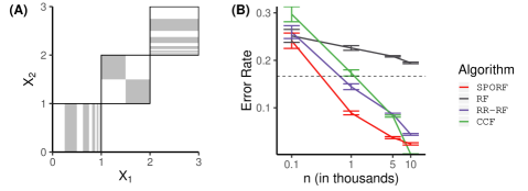
Figure 1: Classification performance on the consistency ($p=2$) problem as a function of the number of training samples. The consistency problem is designed such that RF has a theoretical lower bound of error of 1/6. (A) The joint distribution of $(X,Y)$. $X$ is uniformly distributed in the three unit squares. The lower left and upper right squares have countably infinite stripes (a finite number of stripes are shown), and the center square is a $2\times 2$ checkerboard. The white areas represent $f(X)=0$ and gray areas represent $f(X)=1$. (B) Error rate as a function of $n$. The dashed line represents the lower bound of error for RF, which is 1/6. Sporf and other oblique methods achieve an error rate dramatically lower than the lower bound for RF.

4.2 Simulated datasets

In the sections that follow, we perform a variety of experiments on three carefully constructed simulated classification problems, refered to as Sparse Parity, Orthant, and Trunk. These constructions were chosen to highlight various properties of different algorithms and gain insight into their behavior.

Sparse Parity is a multivariate generalization of the noisy XOR problem. It is a $p$-dimensional two-class problem in which the class label $Y$ is $0$ if the number of dimensions having positive values amongst the first $p^{*}<p$ dimensions is even and $Y=1$ otherwise. Thus, only the first $p^{*}$ dimensions carry information about the class label, and no subsets of dimensions contains any information. Specifically, let $X=(X_{1},\ldots,X_{p})$ be a $p$-dimensional feature vector, where each $X_{1},\ldots,X_{p}\overset{iid}{\sim}U(-1,1)$. Furthermore, let $Q=\sum_{j=1}^{p^{*}}{\mathbb{I}(X_{j}>0)}$, where $p^{*}<p$ and $\mathbb{I}(X_{j}>0)$ is the indicator that the $j^{th}$ feature has a value greater than zero. A sample’s class label $Y$ is equal to the parity of $Q$. That is, $Y=\texttt{odd}(Q)$, where odd returns 1 if its argument is odd, and 0 otherwise. The Bayes optimal decision boundary for this problem is a union of hyperplanes aligned along the first $p^{*}$ dimensions. For the experiments presented in the following sections, $p^{*}=3$ and $p=20$. Figure 2 (A,B) show cross-sections of the first two dimensions taken at two different locations along the third dimension. This setting is designed to be relatively easy for F-RC, but relatively difficult for RF.

Orthant is a multi-class problem in which the class label is determined by the orthant in which a datapoint resides. An orthant in $\mathbb{R}^{p}$ is a generalization of a quadrant in $\mathbb{R}^{2}$. In other words, each orthant is a subset of $\mathbb{R}^{p}$ defined by constraining each of the $p$ coordinates to be positive or negative. For instance, in $\mathbb{R}^{2}$, there are four such subsets: $X=(X_{1},X_{2})$ can either be in 1) $\mathbb{R}^{+}\times\mathbb{R}^{+}$, 2) $\mathbb{R}^{-}\times\mathbb{R}^{+}$, 3) $\mathbb{R}^{-}\times\mathbb{R}^{-}$, or 4) $\mathbb{R}^{+}\times\mathbb{R}^{-}$ . Note that the number of orthants in $p$ dimensions is $2^{p}$. A key characteristic of this problem is that the individual dimensions are strongly and equally informative. Specifically for our experiments, we sample each $X_{1},\ldots,X_{p}\overset{iid}{\sim}U(-1,1)$. Associate a unique integer index from $1$ to $2^{p}$ with each orthant, and let $O(X)$ be the index of the orthant in which $X$ resides. The class label is $Y=O(X)$. Thus, there are $2^{p}$ classes. The Bayes optimal decision boundary in this setting is a union of hyperplanes aligned along each of the $p$ dimensions. We set $p=6$ in the following experiments. Figure 2 (D,E) show cross-sections of the first two dimensions taken at two different locations along the third dimension. This setting is designed to be relatively easy for RF because all optimal splits are axis-aligned.

Trunk is a balanced, two-class problem in which each class is distributed as a $p$-dimensional multivariate Gaussian with identity covariance matrices [31]. Every dimension is informative, but each subsequent dimension is less informative than the last. The class 1 mean is $\mu_{1}=(1,\frac{1}{\sqrt{2}},\frac{1}{\sqrt{3}},...,\frac{1}{\sqrt{p}})$, and $\mu_{0}=-\mu_{1}$. The Bayes optimal decision boundary is the hyperplane $(\mu_{1}-\mu_{0})^{\mathsf{T}}X=0$. We set $p=10$ in the following experiments.

4.3 Sporf Combines the Best of Existing Axis-Aligned and Axis-Oblique Methods

We compare error rates of RF, Sporf, F-RC, and CCF on the sparse parity and orthant problems. Training and tuning are performed as described in Section 3.2. Error rates are estimated by taking a random sample of size $n$, training the classifiers, and computing the fraction misclassified in a test set of 10,000 samples. This is repeated ten times for each value of $n$. The reported error rate is the mean over the ten repeated experiments.

Sporf performs as well as or better than the other algorithms on both the sparse parity (Figure 2C) and orthant problems (Figure 2F). RF performs relatively poorly on the sparse parity problem. Although the optimal decision boundary is a union of axis-aligned hyperplanes, each dimension is completely uninformative on its own. Since axis-aligned partitions are chosen one at a time in a greedy fashion, the trees in RF struggle to learn the correct partitioning. On the other hand, oblique splits are informative, which substantially improves the generalizability of Sporf and F-RC. While F-RC performs well on the sparse parity problem, it performs much worse than RF and Sporf on the orthant problem. On the orthant problem, in which RF is is designed to do exceptionally well, Sporf performs just as well. CCF performs poorly on both problems, which may be because CCA is not optimal for the particular data distributions. For instance, in the sparse parity problem, the projection found by CCA at the first node is approximately the difference in class-conditional means, which is zero. Furthermore, CCF only evaluates $d=min(l,C-1)$ projections at each split node, where $l$ is the number of dimensions subsampled and $C$ is the number of classes. On the other hand, Sporf evaluates $d$ random projections, and $d$ could be as large as $3^{p}$ (each of the $p$ elements can be either $0$ or $\pm 1$. Overall, Sporf is the only method of the four that performs relatively well on all of the simulated data settings.

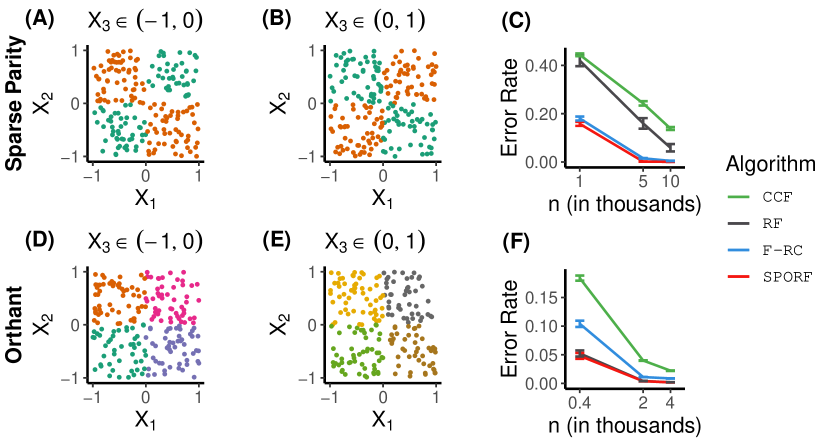
Figure 2: Classification performance on the sparse parity ($p_{s}=20$) and orthant ($p_{o}=6$) problems for various numbers of training samples. In both case, we sample $X_{1},\ldots,X_{p}\overset{iid}{\sim}U(-1,1)$. F-RC has been known to perform much better than RF on the sparse parity problem [10]. The orthant problem is designed for RF to perform well because the optimal splits are axis-aligned. (A) A cross-section of the first two dimensions of sparse parity when $X_{3}\in(-1,0)$. Only the first three dimensions are informative w.r.t. class label. (B) The same as (A), except that the cross-section is taken over $X_{3}\in(0,1)$. (C) Error rate plotted against the number of training samples for sparse parity. Error rate is the average over ten repeated experiments. Error bars indicate the standard error of the mean. (D)-(F) Same as (A)-(C) except for the orthant problem. Sporf is the only method of the four that performs well across all simulated data settings.

4.4 Sporf is Robust to Hyperparameter Selection

One key difference between the random projection distribution of Sporf and F-RC is that F-RC requires that a hyperparameter be specified to fix the sparsity of the sampled univariate projections (i.e., individual linear combinations). Breiman denoted this hyperparameter as $L$. Sporf on the other hand, requires that sparsity be specified on the entire random matrix $\mathbf{A}$, and hence, only an average sparsity on the univariate projections (details are in Section 3.1). In other words, Sporf induces a probability distribution with positive variance on the sparsity of univariate projections, whereas in F-RC that distribution is a point mass. If the Bayes optimal decision boundary is locally sparse, mis-specification of the hyperparameter controlling the sparsity of $\mathbf{A}$ may be more detrimental to F-RC than Sporf. Therefore, we examine the sensitivity of classification performance of Sporf and F-RC to the sparsity hyperparameter $\lambda$ on the simulated datasets described previously. For Sporf, $\lambda$ is defined as in Section 3.1. For F-RC, we note that $\lambda=L/p$ (i.e. density of a univariate projection is the number of features to combine, divided by the total number of features). For each of $\lambda\in\{\frac{2}{p},\ldots,\frac{5}{p}\}$, the best performance for each algorithm is selected with respect to the hyperparameter based on minimum out-of-bag error. Error rate on the test set is computed for each of the four hyperparameter values for the two algorithms. Figure 3 shows the dependence of error rates of Sporf and F-RC on $\lambda$ for the Sparse Parity ($n$ = 5,000) and Orthant ($n=400$) settings. The $n$ = 5,000 setting for Sparse Parity was chosen because both F-RC and Sporf perform well above chance (see Figure 2C). The $n$ = 400 setting for Orthant was chosen for the same reason and also because it displays the largest difference in classification performance in Figure 2F. In both settings, Sporf is more robust to the choice of sparsity level than F-RC.

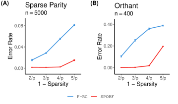
Figure 3: Dependence of error rate on the hyperparameter $\lambda$, which controls the average density (1 - sparsity) of projections for two different simulation settings. (A) Error rate as a function of $\lambda$ on sparse parity ($n=5000$, $p=20$). (B) The same as (A) except on orthant ($n=400$, $p=6$). In both cases, Sporf is less sensitive to different values of $\lambda$ than is F-RC.

4.5 Sporf Learns Important Features

For many data science applications, understanding which features are important is just as critical as finding an algorithm with excellent predictive performance. One of the reasons RF is so popular is that it can learn good predictive models that simultaneously lend themselves to extracting suitable feature importance measures. One such measure is the mean decrease of Gini importance (hereafter called Gini importance) [9]. This measure of importance is popular because of its computational efficiency: it can be computed during training with minimal additional computation. For a particular feature, it is defined as the sum of the reduction in Gini impurity over all splits of all trees made on that feature. With this measure, features that tend to yield splits with relatively pure nodes will have large importance scores. When using RF, features with low marginal information about the class label, but high pairwise or other higher-order joint distributional information, will likely receive relatively low importance scores. Since splits in Sporf are linear combinations of the original features, such features have a better chance of being identified. For Sporf, we compute Gini importance for each unique univariate projection (i.e. single linear combination). Of note, two projections that differ only by a sign, project into the same subspace. However, in the experiment that follows we do not check whether any two projections used in the grown forest differ only by a sign.

Another measure of feature importance which we do not consider here is the permutation importance. Permutation importance of a particular feature is computed by shuffling the values along that feature and subsequently assessing how much the error rate increases using the shuffled feature to predict (relative to intact). This measure is considerably slower to compute than is Gini importance in high-dimensional settings because predictions are made for each permuted feature. Furthermore, it is unclear to us how to appropriately compute permutation importance for linear combinations of features.

Another advantage of Sporfis that methods such as F-RC ,RR-RF and CCF do not lend themselves to computation of Gini importance. The reason for this is that a particular univariate projection must be sampled and chosen many times over many trees in order to compute a stable estimate of its Gini importance. Since the aforementioned algorithms randomly sample continuous coefficients, it is extremely improbable that the same exact univariate projections will be sampled more than once across trees. On the other hand, the projections sampled in Sporf are sparse and only contain coefficients of $\pm 1$, making it much more likely to sample any given univariate projection repeatedly. Furthermore, RR-RF and CCF split on dense univariate projections, which tend to be uninterpretable.

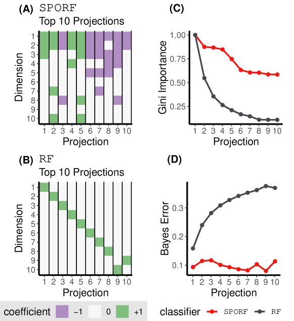
Figure 4: The ten projections with the highest Gini importance found by RF and Sporf on the Trunk problem with $p=10,n=1000$. (A) Visual representation of the top 10 projections identified by Sporf. The x-axis indicates the projection. The y-axis indicates the index of the ten canonical dimensions. The colors in the heat map indicate the linear coefficients of each canonical dimension that define each of the projections. (B) The same as (A), except for RF. (C) Comparison of the Gini importances of the 10 best projections found by each algorithm. (D) Comparison of the Bayes error rate of the 10 best projections found by each algorithm. The top 10 projections used in Sporf all have substantially lower Bayes error than those used in RF, indicating that Sporf learns interpretable informative features.

Gini importance was computed for each feature for both RF and Sporf on the Trunk problem with $n=1,000$. Figure 4 depicts the features that define each of the top ten split node projections for Sporf (A) and RF (B). Projections are sorted from highest to lowest Gini importance. The top ten projections in Sporf are all linear combinations of dimensions, whereas in RF the projections can only be along single dimensions. The linear combinations in Sporf tend to include the first few dimensions, which contain most of the “true” signal. The best possible projection that Sporf could sample is the vector of all ones. However, since $\lambda=1/2$ for this experiment, the probability of sampling such a dense projection is almost negligible. Figure 4(C) shows the normalized Gini importance of the top ten projections for each algorithm. The top ten most important features according to Sporf are all more important (in terms of Gini) than any of the RF features, except the very first one. Figure 4(D) shows the Bayes error rate of the top ten projections for each algorithm. Again, the top ten features according to Sporf are more informative than any of those according to RF. In other words, Sporf learns features that are more important than any of the observed features, and those features are interpretable, as they are sparse linear combinations of the observed features. The ability of Sporf to learn new identifiable features distinguishes it from RF, which cannot learn new features.

5 Real Data Empirical Performance

5.1 Sporf Exhibits Best Overall Classification Performance on a Large Suite of Benchmark Datasets

Sporf compares favorably to RF, XGBoost, RR-RF, and CCF on a suite of 105 benchmark datasets from the UCI machine learning repository (Figure 5). This benchmark suite is a subset of the same problem sets previously used to conclude that RF outperformed $>$100 other algorithms [1] (16 were excluded for various reasons such as lack of availability; see Appendix B for preprocessing details).

Figure 5(A) shows pairwise comparisons of RF with Sporf (red), XGBoost (yellow), RR-RF (purple), and CCF (green) on the UCI datasets. Specifically, let $\kappa(\cdot)$ denote Cohen’s kappa (fractional decrease in error rate over the chance error rate) for a particular classification algorithm. Here, error rates are estimated for each algorithm for each dataset via five-fold cross-validation. Error rates for each data set are reported in Appendix F. Let $\Delta(\mathcal{A})=\kappa({\sc\texttt{RF}})-\kappa(\mathcal{A})$ be the difference between $\kappa$ for some algorithm $\mathcal{A}$—either Sporf, XGBoost, RR-RF, or CCF—with $\kappa({\sc\texttt{RF}})$. Each beeswarm plot in 5(A) represents the distribution of $\Delta(\mathcal{A})$, denoted "Effect Size," over data sets. Comparisons are shown for the 65 numeric datasets (top), the 40 datasets having at least one categorical feature (middle), and all 105 datasets (bottom). A positive value on the x-axis indicates that RF performed better than the algorithm it is being compared to on a particular dataset, while a negative value indicates it performed worse. Values on the y-axis greater than 10% were squashed to 10% and values less than -10% were squashed to -10% in order to improve visualization. Mean values are indicated by a black "x." As indicated by the downward skewing distribution, Sporf tends to outperform RF over all datasets, due in particular to its relative performance on the numeric datasets. RR-RF and CCF also tend to perform similar to or better than RF on the numeric datasets, but unlike Sporf they perform worse than RF on the categorical datasets; the oblique methods are likely sensitive to the one-hot encoding of categorical features. $\kappa$ values for individual data sets and algorithms can be found in Table LABEL:tab:class.

Additionally, we examined how frequently each algorithm ranked in terms of $\kappa$ across the datasets. A rank of one indicates first place (best) on a particular dataset and a rank of five indicates last place (worst). Histograms (in fraction of data sets) of the relative ranks are shown in Figure 5(B). Overall, Sporf tends to outperform the other algorithms. This is despite the fact that XGBoost is tuned significantly more than Sporf in these comparisons (see Section 3.2 for details). Surprisingly, we find that RR-RF, one of the most recent methods to be proposed, has a strong tendency to perform the worst. One-sided Wilcoxon signed-rank tests were performed to determine whether Sporf performed significantly better than each of the other algorithms. Specifically, the null hypothesis was that the median $\kappa$ value of Sporf is greater than that of each algorithm being compared to. P-values are shown for each algorithm compared with Sporf to the right of each histogram in Figure 5(B). Over all data sets, we found that p-values were $<0.005$ for every algorithm compared with Sporf.

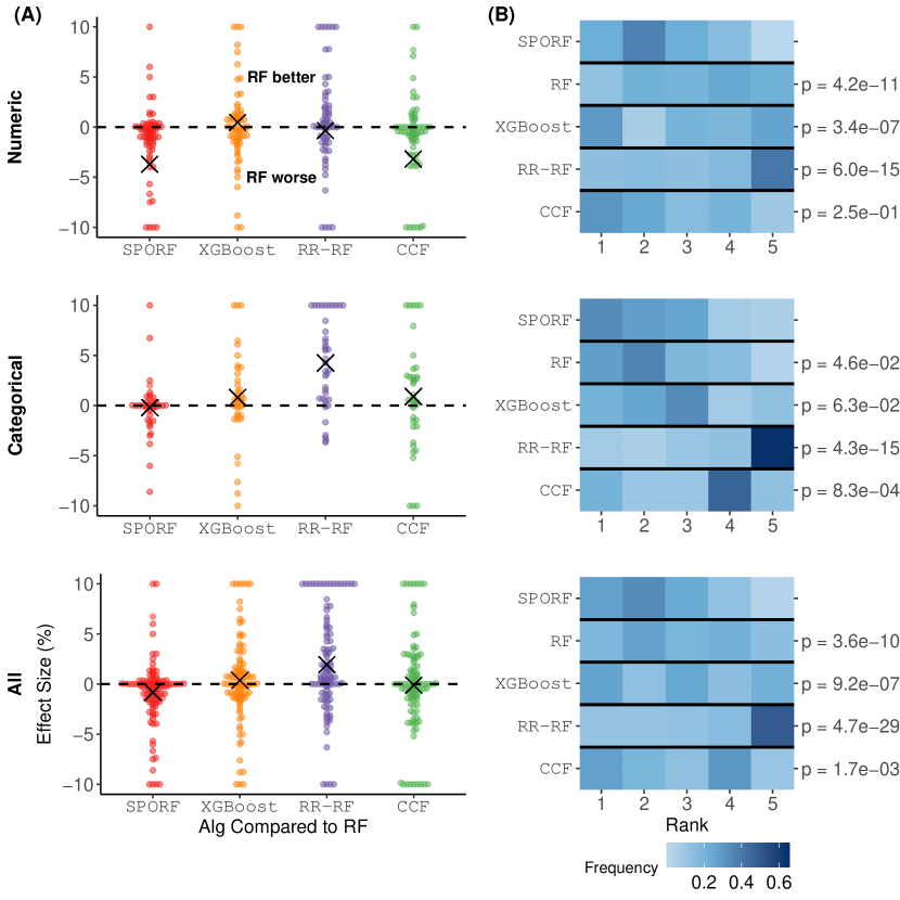
Figure 5: Pairwise comparisons of RF with Sporf, XGBoost, RR-RF, and CCF on the numeric datasets (top), categorical datasets (middle), and all datasets (numeric and categorical combined; bottom) from the UCI Machine Learning Repository (105 datasets total). (A) Beeswarm plots showing the distributions of classification performance relative to RF for various decision forest algorithms. Classification performance is measured by effect size, which is defined as $\kappa({\sc\texttt{RF}})-\kappa(\mathcal{A})$, where $\kappa$ is Cohen’s kappa and $\mathcal{A}$ is one of the algorithms compared to RF. Each point corresponds to a particular data set. Mean effect sizes are indicated by a black ”x.” A negative value on the y-axis indicates RF performed worse than a particular algorithm. (B) Histograms of the relative ranks of the different algorithms, where a rank of 1 indicates best relative classification performance and 5 indicates worst. Color indicates frequency, as fraction of data sets. P-values correspond to testing that RF, XGBoost, RR-RF, and CCF performed worse than Sporf, using one-sided Wilcoxon signed-rank tests. Overall, Sporf tends to perform better than the other algorithms.

5.2 Identifying Default Hyperparameter Settings

While the hyperparameters $\lambda$ and $d$ of Sporf were tuned in this comparison, default hyperparameters can be of great value to researchers who use Sporf out of the box. This is especially true for those not familiar with the details of a particular algorithm or those having limited time and computational budget. Therefore, we sought suitable default values for $\lambda$ and $d$ based on classification performance on the UCI datasets. For each dataset, for each fold the hyperparameter settings are ranked based on Cohen’s kappa computed on the held out set. A rank of $n$ indicates $n^{th}$ place (i.e. first place indicates largest kappa). Ties in the ranking procedure are handled by assigning all ties the same averaged rank. For example, consider the set of real numbers $\{a_{1},a_{2},a_{3}\}$ such that $a_{1}>a_{2}=a_{3}$. Then $a_{1}$ would be assigned a rank of three and $a_{2}$ and $a_{3}$ would both be assigned a rank of $(1+2)/2=1.5$. The rank of each hyperparameter pair was averaged over the five folds. Finally, for each hyperparameter pair, the median rank is computed over the datasets. The median rank for each hyperparameter setting is depicted in Figure 6. The results here suggest that $d=p^{2}$ and $\lambda=4/p$ is the best default setting for Sporf with respect to classification performance. However, we choose the setting $d=p$ and $\lambda=3/p$ as the default values in our implementation because it requires substantially less training time for moderate to large $p$ at the expense of only a slightly greater tendency to perform worse on the UCI datasets.

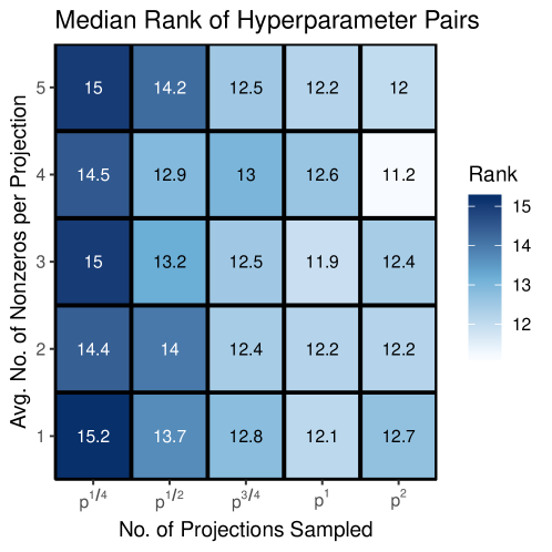
Figure 6: Median rank of Sporf’s ($d$, $\lambda$) hyperparameter pairs on the UCI classification datasets (lower is better). Although $(p^{2},4/p)$ is the best performance-wise, we select $(p,3/p)$ as the default because of a good balance between accuracy and training time.

5.3 Sporf is Robust to High-Dimensional Noise

Next, we investigated the effect of adding a varying number of noise dimensions to the UCI benchmark datasets. For each of the 105 UCI datasets used in the previous experiment, $D_{noise}$ standard Gaussian dimensions were appended to the input matrix, for $D_{noise}\in\{10,100,1000\}$. Algorithm comparisons were then performed in the same way as before.

Figure 7 shows the overall classification performance of Sporf, RF, XGBoost, and CCF for each value of $D_{noise}$. Each of the points plotted represents the mean Cohen’s kappa ($\pm$ SEM) over all datasets. For all values of $D_{noise}$, Sporf ties for best classification performance. Notably, CCF performs about as well as Sporf when there is little or no additional noise, but degrades substantially when many noise dimensions are added. This suggests that using supervised linear procedures to compute splits may lead to poor out-of-sample performance, likely because the learned features have overfit to the noise dimensions. RR-RF degrades even more rapidly than does CCF with increasing numbers of noise dimensions. This can be explained by the fact that features derived from random rotations, which are dense linear projections, have very low probability of being informative in the presence of many noise dimensions.

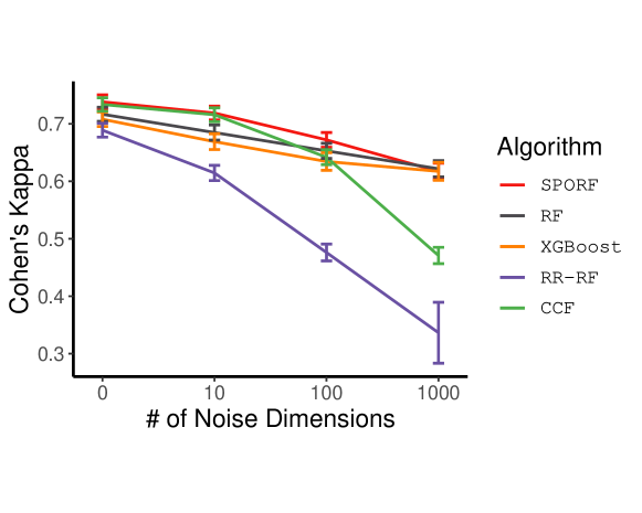
Figure 7: Comparison of classification performance on the UCI benchmark datasets with a varying number of Gaussian noise dimensions added. The x-axis represents the number of noise dimensions added. The y-axis represents the average of Cohen’s kappa value over all datasets ($\pm SEM$). Sporf is always tied for the best performance. CCF and RR-RF are more sensitive to additional noise dimensions.

6 Computational Efficiency and Scalability of Sporf

Computational efficiency and scalability are often as important as accuracy in the choice of machine learning algorithms, especially for big data. In this section we demonstrate that Sporf, with an appropriate choice of hyperparameter settings, scales similarly to RF with respect to sample size and number of features. Furthermore, we show that our open source implementation is computationally competitive with leading implementations of decision tree ensemble algorithms.

6.1 Theoretical Time Complexity

The time complexity of an algorithm characterizes how the theoretical processing time for a given input relies on both the hyper-parameters of the algorithm and the characteristics of the input. Let $T$ be the number of trees, $n$ the number of training samples, $p$ the number of features in the training data, and $d$ the number of features sampled at each split node. The average case time complexity of constructing an RF is $\mathcal{O}(Tdn\log^{2}{n})$ [32]. The $dn\log{n}$ accounts for the sorting of $d$ features at each node. The additional $\log{n}$ accounts for both the reduction in node size at lower levels of the tree and the average number of nodes produced. RF’s near linear complexity shows that a good implementation will scale nicely with large input sizes, making it a suitable algorithm to process big data. Sporf’s average case time complexity is similar to RF’s, the only difference being that there is an additional term representing a sparse matrix multiplication that is required in each node. This makes Sporf’s complexity $\mathcal{O}(Tdn\log^{2}{n}+Tdnp\lambda))$, where $\lambda$ is the fraction of nonzeros in the $p\times d$ random projection matrix. We generally let $\lambda$ be close to $1/p$, giving a complexity of $\mathcal{O}(Tdn\log^{2}{n})$, which is the same as for RF. Of note, in RF $d$ is constrained to be no greater than $p$, the dimensionality of the data. Sporf, on the other hand, does not have this restriction on $d$. Therefore, if $d$ is selected to be greater than $p$, Sporf may take longer to train. However, $d>p$ often results in improved classification performance.

6.2 Theoretical Space Complexity

The space complexity of an algorithm describes how the theoretical maximum memory usage during runtime scales with the number of inputs and hyperparameters. Let $c$ be the number of classes and $T$, $p$, and $n$ be defined as in Section 6.1. Building a single tree requires the data matrix to be kept in memory, which is $\mathcal{O}(np)$. During an attempt to split a node, two $c$-length arrays store the counts of each class to the left and to the right of the candidate split point. These arrays are used to evaluate the decrease in Gini impurity or entropy. Additionally, a series of random sparse projection vectors are sequentially assessed. Each vector has less than $p$ nonzeros. Therefore this term is dominated by the $np$ term. Assuming trees are fully grown, meaning each leaf node contains a single data point, the tree has $2n$ nodes in total. This term gets dominated by the $np$ term as well. Therefore, the space complexity to build a Sporf is $\mathcal{O}(T(np+c))$. This is the same as that of RF.

6.3 Theoretical Storage Complexity

Storage complexity is the disk space required to store a forest, given the inputs and hyperparameters. Assume that trees are fully grown. For each leaf node, only the class label of the training data point contained within the node is stored, which is $\mathcal{O}(1)$. For each split node, the split dimension index and threshold are stored, which are also both $\mathcal{O}(1)$. Therefore, the storage complexity of a RF is $\mathcal{O}(Tn)$.

For a Sporf, the only aspect that differs is that a (sparse) vector is stored at each split node rather than a single split dimension index. Let $z$ denote the average number of nonzero entries in a vector projection stored at each split node. Storage of this vector at each split node requires $\mathcal{O}(z)$ memory. Therefore, the storage complexity of a Sporf is $\mathcal{O}(Tnz)$. $z$ is a random variable whose prior is governed by $\lambda$, which is typically set to $1/p$. The posterior mean of $z$ is determined also by the data; empirically it is close to $z=1$. Therefore, in practice, the storage complexity of Sporf is close to that of RF.

6.4 Empirical Computational Efficiency and Scalability

6.5 Implementation Details

We use our own R implementation for evaluations of RF, Sporf, F-RC, and RR-RF [33]. It was more difficult to modify one of the existing popular tree learning implementations due to the particular way in which they operate on the input data. In all of the popular axis-aligned tree learning implementations, each feature in the input data matrix is sorted just once prior to inducing a tree, and the tree induction procedure operates directly on this presorted data. Since trees in a Sporf include splitting on new features consisting of linear combinations of the original features, pre-sorting the data is not an option. Therefore our implementation is written from scratch in mostly native R. The code has been extensively profiled and optimized for speed and memory performance. Profiling revealed the primary performance bottleneck to be the portion of code responsible for finding the best split. In order to improve speed, this portion of code was implemented in C++ and integrated into R using the Rcpp package [34]. Further speedup is achieved through multicore parallelization of tree construction and byte-compilation via the R compiler package.

XGBoost is evaluated using the R implementation available on CRAN [35]. CCF is evaluated using the authors’ openly available MATLAB implementation [7].

6.5.1 Comparison of Algorithms Using the Same Implementation

Figure 8(A) shows the training times of RF, F-RC, and Sporf on the sparse parity problem. The reported training times correspond to the best hyperparameter settings for each algorithm. Experiments are run using an Intel Xeon E5-2650 v3 processors clocked at 2.30GHz with 10 physical cores, 20 threads, and 250 GB DDR4-2133 RAM. The operating system is Ubuntu 16.04. F-RC is the slowest, RF is the fastest, and Sporf is in between. While not shown, we note that a similar trend holds for the orthant problem. Figure 8(B) shows that when the hyperparameter $d$ of Sporf and F-RC is the same as that for RF, training times are comparable. However, training time continues to increase as $d$ exceeds $p$ for Sporf and F-RC, which largely accounts for the trend seen in Figure 8(A). Figure 8(C) indicates that this additional training time comes with the benefit of substantially improved accuracy. Restricting $d$ to be no greater than $p$ for Sporf in this setting would still perform noticeably better than RF at no additional cost in training time. Therefore, Sporf does not trade off accuracy for time. Rather, for a fixed computational budget, it achieves better accuracy, and if allowed to use more computation, further improves accuracy.

Sparse Parity

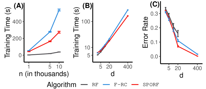
Figure 8: Comparison of training times of RF, Sporf, and F-RC on the 20-dimensional sparse parity setting. (A) Dependency of training time using the best set of hyperparameters (y-axis) on the number of training samples (x-axis) for the sparse parity problem. (B) Dependency of training time (y-axis) on the number of projections sampled at each split node (x-axis) for the sparse parity problem with $n=5000$. (C) Dependency of error rate (y-axis) on the number of projections sampled at each split node (x-axis) for the sparse parity problem with $n=5000$. Sporf and F-RC can sample many more than $p$ projections, unlike RF. As seen in panels (B) and (C), increasing $d$ above $p$ meaningfully improves classification performance at the expense of larger training times. However, comparing error rates and training times at $d=20$, Sporf can classify substantially better than RF even with no additional cost in training time.

6.5.2 Comparison of Training and Prediction Times for Different Implementations

We developed and maintain an open multi-core R implementation of Sporf , which is hosted on CRAN [33]. We compare both speed of training and strong scaling of our implementation to those of the R Ranger [36] and XGBoost [35] packages, which are currently two of the fastest, parallelized decision tree ensemble software packages available. Strong scaling is the time needed to train a forest with one core divided by the time needed to train a forest with multiple cores. Ranger offers a fast multicore version of RF that has been extensively optimized for runtime performance. XGBoost offers a fast multicore version of gradient boosted trees, and computational performance is optimized for shallow trees. Both Ranger and XGBoost are C++ implementations with R wrappers, whereas our Sporf implementation is almost entirely native R. Hyperparameters are chosen for each implementation so as to make the comparisons fair. For all implementations, trees are grown to full depth, 100 trees are constructed, and $d=\sqrt{p}$ features sampled at each node. For Sporf, $\lambda=1/p$. Experiments are run using four Intel Xeon E7-4860 v2 processors clocked at 2.60GHz, each processor having 12 physical cores and 24 threads. The amount of available memory is 1 TB DDR3-1600. The operating system is Ubuntu 16.04. Comparisons use three openly available large datasets:

MNIST

The MNIST dataset [37] has 60,000 training observations and 784 (28x28) features. For a small number of cores, Sporf is faster than XGBoost but slower than Ranger (Figure 9(A)). However, when 48 cores are used, Sporf is as fast as Ranger and still faster than XGBoost.

Higgs

The Higgs dataset (https://www.kaggle.com/c/higgs-boson) has 250,000 training observations and 31 features. Sporf is as fast as ranger and faster than XGBoost when using 48 cores (Figure 9(B)).

p53

The p53 dataset (https://archive.ics.uci.edu/ml/datasets/p53+Mutants) has 31,159 training observations and 5,409 features. Figure 9(C) shows a similar trend as for MNIST. For this dataset, utilizing additional resources with Sporf does not provide as much benefit due to the classification task being too easy (all algorithms achieve perfect classification accuracy)—the trees are shallow, causing the overhead cost of multithreading to outweigh the speed increase as a result of parallelism.

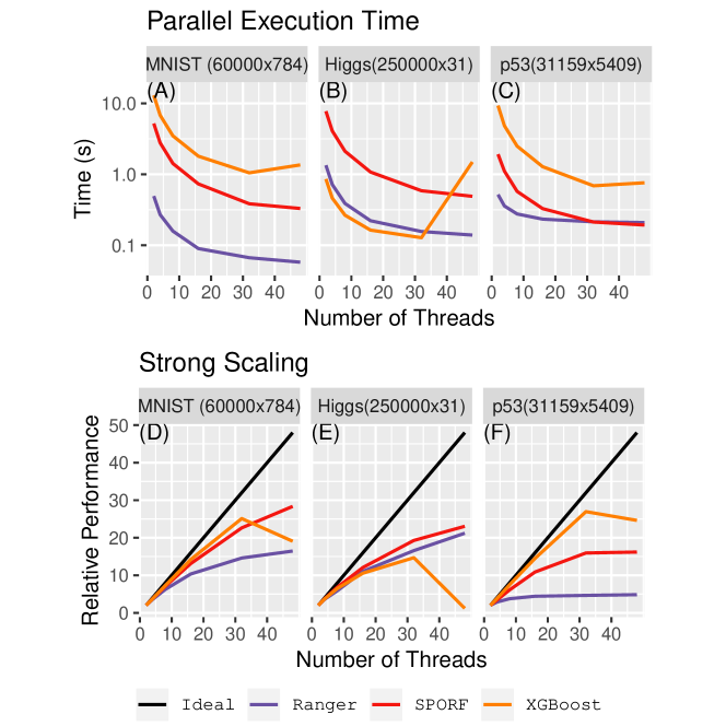
Figure 9: (A-C) The per-tree training time for three large real world datasets. Training was performed using matching parameters where possible, and default parameters otherwise. Sporf’s performance—even though it is written mostly in native R, as compared to the other optimized C++ codes—is comparable to the highly optimized XGBoost and Ranger and even outperforms XGBoost on two of the datasets. (D-F): Strong scaling is the time needed to train a forest with one core divided by the time needed to train a forest with multiple cores. This is a measurement of a system’s ability to efficiently utilize additional resources. Sporf is able to scale well over the entire range of tested cores, whereas XGBoost has sharp drops in scalability during which it is unable to use additional threads due to characteristics of the given datasets. The p53 dataset, despite having a large number of dimensions, is easily classifiable, which leads to short trees. The p53 strong scaling plot shows that when trees are short, the overhead of multithreading prevents Sporf from efficiently using the additional resources.

Strong scaling is the relative increase in speed of using multiple cores over that of using a single core. In the ideal case, the use of $N$ cores would produce a factor $N$ speedup. Sporf has the best strong scaling on MNIST (Figure 9(D)) and Higgs (Figure 9(E)), while it has strong scaling in between that of Ranger and XGBoost on the p53 data set (Figure 9(F)). This is due to the simplicity of the p53 dataset, as discussed above.

Prediction times can be just as, or even more important than training times in certain applications. For example, electron microscopy-based connectomics can acquire multi-petabyte datasets that require classification of each voxel [38]. Moreover, recent automatic hyperparameter tuning suites incorporate runtime in their evaluations, which leverage out-of-sample prediction accuracy [39]. Thus, accelerating prediction times can improve the effectiveness of hyperparameter sweeps.

Figure 10 compares the prediction times of the various implementations on the same three datasets. In addition to our standard Sporf prediction implementation, we also compare a "Forest Packing" prediction implementation [40]. Briefly, Forest Packing is a procedure performed after a forest has been grown that reduces prediction latency by reorganizing and compacting the forest data structure. The number of test points used for the Higgs, MNIST, and p53 datasets is 50,000, 10,000, and 6,000, respectively. Predictions were made sequentially without batching using a single core. Sporf is significantly faster than Ranger on the Higgs and MNIST datasets, and only marginally slower on the p53 dataset. XGBoost is much faster than both Sporf and Ranger, which is due to the fact that the XGBoost algorithm constructs much shallower trees than the other methods. Most notably, the Forest Packing procedure, which "packs" the trees learned by Sporf, makes predictions roughly ten times faster than XGBoost and over 100 times faster than the standard Sporf on all three datasets.

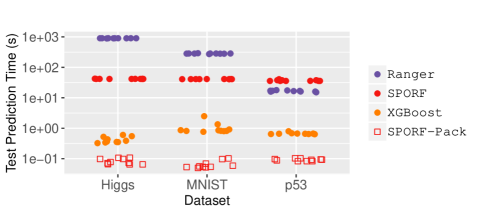
Figure 10: Comparison of test set prediction times. Forest Packing results show a 10x speed up in real time prediction scenarios. Test set sizes: Higgs, 50,000 observations; MNIST, 10,000 observations; p53, 6,000 observations. Predictions were made sequentially without batching.

7 Conclusion

In this work we showed that existing oblique splitting extensions to RF forfeit some of the nice properties of RF, while achieving improved performance in certain settings. We therefore introdced Sporf which was designed to preserve the desirable properties of both RF and oblique forest methods, rendering it statistically robust, computationally efficient, scalable, and interpretable. This work only focused on classification; we also have a preliminary implementation for regression, which seems to perform similarly to RF on a suite of regression benchmark data sets. Future work will investigate the behavior and performance of Sporf on univariate and multivariate regression tasks.

One limitation of using sparse random projections to generate the candidate oblique splits is that it will never find informative splits in cases for which the signal is contained in a dense linear combination of features or nonlinear combinations of features. In such cases, supervised computation of split directions may be more suitable. Perhaps a decision forest method that evaluates both sparse random projections and dense supervised projections at each split node could further improve performance in such settings.

On a more theoretical note, we demonstrated that Sporf achieves empirical statistical consistency on a classification problem for which Biau et al. [30] proved that RF cannot achieve better than an error rate of 1/6, even though the Bayes optimal error rate is zero in this setting. This raises a question as to whether it is possible to construct a problem in which RF is consistent and Sporf is not. Or could it be the case that Sporf is always consistent when RF is? The consistency theorems in Biau et al. [41] for RF in the case of additive regression models should be extendable to Sporf with some minor modifications—their proofs rely on clever adaptations of classical consistency results for data-independent partitioning classifiers, which are agnostic to whether the splits are axis-aligned or not. Another factor that dictates the lower bound of error rate, as Breiman [5] proved, is the relative balance between the strength and correlation of trees. Our investigation of strength and correlation on the Sparse Parity, Orthant, and Trunk simulations is offered in Appendix C. The results suggest that Sporf can outperform other algorithms because of stronger trees and/or less correlated trees. Therefore, Sporf perhaps offers more flexible control over the balance between tree strength and correlation, thereby allowing it to adapt better to different problems.

Our implementation of Sporf is as computationally efficient and scalable or more so than existing tree ensemble implementations. Additionally, our implementation can realize many previously proposed tree ensemble methods by allowing the user to define how random projections are generated. Open source code is available at https://neurodata.io/sporf/, including both the R package discussed here, and a C++ version with both R and Python bindings that we are actively developing.

Appendix A Hyperparameter Tuning

Hyperparameters in XGBoost are tuned via grid search using the R caret package. The values tried for each hyperparameter are based on suggestions by Owen Zhang (https://www.slideshare.net/OwenZhang2/tips-for-data-science-competitions), a research data scientist who has had many successes in data science competitions using XGBoost:

• nrounds: 100, 1000

• subsample: 0.5, 0.75, 1

• eta: 0.001, 0.01

• colsample_bytree: 0.4, 0.6, 0.8, 1

• min_child_weight: 1

• max_depth: 4, 6, 8, 10, 100000

• gamma: 0

Selection of the hyperparameter values is based on minimization of a five-fold cross-validation error rate.

Appendix B Real Benchmark datasets

We use 105 benchmark datasets from the UCI machine learning repository for classification. These datasets are most of the datasets used in Fernandez-Delgado et al. [1]; some were removed due to licensing or unavailability issues. We noticed certain anomalies in [1]’s pre-processed data, so we pre-processed the raw data again as follows.

1. Remove of nonsensical features. Some features, such as unique sample identifiers, or features that were the same value for every sample, were removed.

2. Impute missing values. The R randomForest package was used to impute missing values. This method was chosen because it is nonparametric and is one of the few imputation methods that can natively impute missing categorical entries.

3. One-hot-encode categorical features. Most classifiers cannot handle categorical data natively. Given a categorical feature with possible values $\{c_{1},\ldots,c_{m}\}$, we expand to $m$ binary features. If a data point has categorical value $c_{k},\forall k\in 1,\ldots,m$ then the $k^{th}$ binary feature is assigned a value of one and zero otherwise.

4. Integer encoding of ordinal features. Categorical features having order to them, such as "cold", "luke-warm", and "hot", were numerically encoded to respect this ordering with integers starting from 1.

5. Standardization of the format. Lastly, all datasets were stored as CSV files, with rows representing observations and columns representing features. The class labels were placed as the last column.

6. Five-fold parition. Each dataset was randomly divided into five partitions for five-fold cross-validation. Partitions preserved the relative class frequencies by stratification. Each partition included a different $20\%$ of the data for testing.

Appendix C Strength and Correlation of Trees

One of the most important and well-known results in ensemble learning theory for classification states that the generalization error of an ensemble learning procedure is bounded above by the quantity ${\bar{\rho}(1-s^{2})}/{s^{2}}$, where $\bar{\rho}$ is a particular measure of the correlation of the base learners and $s$ is a particular measure of the strength of the base learners [5]. In both Sporf and F-RC, the set of possible splits that can be sampled is far larger in size than that for RF, which may lead to more diverse trees. Moreover, the ability to sample a more diverse set of splits may increase the likelihood of finding good splits and therefore boost the strength of the trees. To investigate the strength and correlation of trees using different projection distributions, we evaluate RF, F-RC, and Sporf on the three simulation settings described above. Scatter plots of tree strength vs tree correlation are shown in Figure 11 for sparse parity ($n=1000$), orthant ($n=400$), Trunk ($n=10$), and Trunk ($n=100$). In all four settings, Sporf classifies as well as or better than RF and F-RC.

On the sparse parity setting, Sporf and F-RC produce significantly stronger trees than does RF, at the expense of an increase in correlation among the trees (Figure 11(A)). Both Sporf and F-RC are much more accurate than RF in this setting, so any performance degradation due to the increase in correlation relative to RF is outweighed by the increased strength. Sporf produces slightly less correlated trees than does F-RC, which may explain why Sporf has a slightly lower error rate than does F-RC on this setting.

On the orthant setting, F-RC produces trees of roughly the same strength as those in RF, but significantly more correlated (Figure 11(B)). This may explain why F-RC has substantially worse prediction accuracy than does RF. Sporf also produces trees more correlated than those in RF, but to a lesser extent than F-RC. Furthermore, the trees in Sporf are stronger than those in RF. Observing that Sporf has roughly the same error rate as RF does, it seems that any contribution of greater tree strength in Sporf is canceled by a contribution of greater tree correlation.

On the Trunk setting with $p=10$ and $n=10$, Sporf and F-RC produces trees that are comparable in strength to those in RF but less correlated (Figure 11(C)). However, when increasing $n$ to $100$, the trees in Sporf and F-RC become both stronger and more correlated. In both cases, Sporf and F-RC have better classification performance than RF.

These results suggest a possibly general phenomenon. Namely, for smaller training set sizes, tree correlation may be a more important factor than tree strength because there is not enough data to induce strong trees, and thus, the only way to improve performance is through increasing the diversity of trees. Likewise, when the training set is sufficiently large, tree correlation matters less because there is enough data to induce strong trees. Since Sporf has the ability to produce both stronger and more diverse trees than RF, it is adaptive to both regimes In all four settings, Sporf never produces more correlated trees than does F-RC, and sometimes produces less correlated trees. A possible explanation for this is that the splits made by Sporf are linear combinations of a random number of dimensions, whereas in F-RC the splits are linear combinations of a fixed number of dimensions. Thus, in some sense, there is more randomness in Sporf than in F-RC.

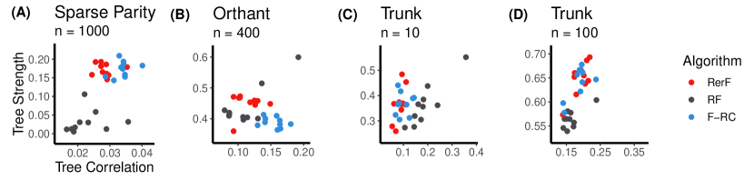
Figure 11: Comparison of tree strength and correlation of Sporf, RF, and F-RC on four of the simulated datasets: (A) sparse parity with $p=10,n=1000$, (B) orthant with $p=6,n=400$, (C) Trunk with $p=10,n=10$, and (D) Trunk with $p=10,n=100$. For a particular algorithm, there are ten dots, each corresponding to one of ten trials. Note in all settings, Sporf beats RF and/or F-RC. However, the mechanism by which it does varies across the different settings. In sparse parity Sporf wins because the trees are substantially stronger, even though the correlation increases. In Trunk for small sample size, it is purely because of less correlated trees. However, when sample size increases 10-fold, it wins purely because of stronger trees. This suggests that Sporf can effectively trade-off strength for correlation on the basis of sample complexity to empirically outperform RF and F-RC.

Appendix D Understanding the Bias and Variance of Sporf

The crux of supervised learning tasks is to optimize the trade-off between bias and variance. As a first step in understanding how the choice of projection distribution effects the balance between bias and variance, we estimate bias, variance, and error rate of the various algorithms on the sparse parity problem. Universally agreed upon definitions of bias and variance for 0-1 loss do not exist, and several such definitions have been proposed for each. Here we adopt the framework for defining bias and variance for 0-1 loss proposed in James [42]. Under this framework, bias and variance for 0-1 loss have similar interpretations to those for mean squared error. That is, bias is a measure of the distance between the expected output of a classifier and the true output, and variance is a measure of the average deviation of a classifier output around its expected output. Unfortunately, these definitions (along with the term for Bayes error) do not provide an additive decomposition for the expected 0-1 loss. Therefore, James [42] provides two additional statistics that do provide an additive decomposition. In this decomposition, the so-called "systematic effect" measures the contribution of bias to the error rate, while the "variance effect" measures the contribution of variance to the error rate. For completeness, we restate these definitions below.

Let $\bar{h}(X)=\operatornamewithlimits{argmax}\limits_{k}P_{\mathcal{D}_{n}}(h(X|\mathcal{D}_{n})=k)$ be the most common prediction (mode) with respect to the distribution of $\mathcal{D}_{n}$. This is referred to as the "systematic" prediction in James [42]. Furthermore, let $P^{*}(X)=P_{Y|X}(Y=h^{*}(X)|X)$ and $\bar{P}(X)=P_{\mathcal{D}_{n}}(h(X|\mathcal{D}_{n})=\bar{h}(X))$. The bias, variance, systematic effect (SE), and variance effect (VE) are defined as

$$Bias =P_{X}(\bar{h}(X)=h^{*}(X)),$$

$$Var =1-E_{X}[\bar{P}(X)],$$

$$SE =E_{X}[P^{*}(X)-P_{Y|X}(Y=\bar{h}(X)|X)],$$

$$VE =E_{X}[P_{Y|X}(Y=\bar{h}(X)|X)$$

$$-\sum\limits_{k}P_{Y|X}(Y=k|X)P_{\mathcal{D}_{n}}(h(X|\mathcal{D}_{n})=k)].$$

Figure 12 compares estimates of bias, variance, variance effect, and error rate for Sporf, RF, and F-RC as a function of number of training samples. Since the Bayes error is zero in these settings, systematic effect is the same as bias. The four metrics are estimated from 100 repeated experiments for each value of $n$. In Figure 12(A), Sporf has lower bias than both RF and F-RC for all training set sizes. All algorithms converge to approximately zero bias after about 3000 samples. Figure 12(B) shows that RF has substantially more variance than do Sporf and F-RC, and Sporf has slightly less variance than F-RC at 3,000 samples. The trend in Figure 12(C) is similar to that in Figure 12(B), which is not too surprising since VE measures the contribution of the variance to the error rate. Interestingly, although RF has noticeably more variance at 500 samples than do Sporf and F-RC, it has slightly lower VE. It is also surprising that the VE of RF increases from 500 to 1000 training samples. It could be that this is the result of the tradeoff of the substantial reduction in bias. In Figure 12(D), the error rate is shown for reference, which is the sum of bias and VE. Overall, these results suggest that Sporf wins on the sparse parity problem with a small sample size primarily through lower bias/SE, while with a larger sample size it wins mainly via lower variance/VE. A similar trend holds for the orthant problem (not shown).

Sparse Parity

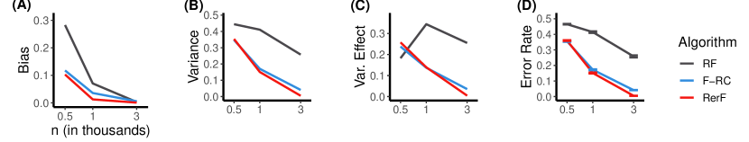
Figure 12: (A-D) Bias, variance, variance effect, and error rate, respectively, on the sparse parity problem as a function of the number of training samples. Error rate is the sum of systematic effect and variance effect, which roughly measure the contributions of bias and variance to the error rate, respectively. In this example, bias and systematic effect are identical because the Bayes error is zero (refer to [42]). For smaller training sets, Sporf wins primarily through lower bias/systematic effect, while for larger training sets it wins primarily through lower variance effect.

Appendix E Algorithms

Algorithm 1 Learning a Sporf classification tree.

1:(1) $\mathcal{D}_{n}=(\mathbf{X},\mathbf{y})\in\mathbb{R}^{n\times p}\times\mathcal{Y}^{n}$: training data (2) $\Theta$: set of split eligibility criteria

2:A Sporf decision tree $T$

3:function $T=$ growtree($\mathbf{X},\mathbf{y},\Theta$)

4:     $c=1$ $\triangleright$ $c$ is the current node index

5:     $M=1$ $\triangleright$ $M$ is the number of nodes currently existing

6:     $S^{(c)}=$ bootstrap($\{1,...,n\}$) $\triangleright$ $S^{(c)}$ is the indices of the observations at node $c$

7:     while $c<M+1$ do $\triangleright$ visit each of the existing nodes

8:         $(\mathbf{X^{\prime}},\mathbf{y^{\prime}})=(\mathbf{x}_{i},y_{i})_{i\in S^{(c)}}$ $\triangleright$ data at the current node

9:         for $k=1,\ldots,K$ do $n_{k}^{(c)}=\sum_{i\in S^{(c)}}I[y_{i}=k]$ end for $\triangleright$ class counts

10:         if $\Theta$ satisfied then $\triangleright$ do we split this node?

11:              $\mathbf{A}=[\mathbf{a}_{1}\cdots\mathbf{a}_{d}]\sim f_{\mathbf{A}}$ $\triangleright$ sample random $p\times d$ matrix as defined in 3.1

12:              $\mathbf{\widetilde{X}}=\mathbf{X^{\prime}}\mathbf{A}=(\mathbf{\widetilde{x}}_{i})_{i\in S^{(c)}}$ $\triangleright$ random projection into new feature space

13:              $(j^{*},t^{*})=$ findbestsplit($\mathbf{\widetilde{X}},\mathbf{y^{\prime}}$) $\triangleright$ Algorithm 2

14:              $S^{(M+1)}=\{i:\mathbf{\widetilde{x}}_{i}\cdot\mathbf{a}_{j^{*}}\leq t^{*}\quad\forall i\in S^{(c)}\}$ $\triangleright$ assign to left child node

15:              $S^{(M+2)}=\{i:\mathbf{\widetilde{x}}_{i}\cdot\mathbf{a}_{j^{*}}>t^{*}\quad\forall i\in S^{(c)}\}$ $\triangleright$ assign to right child node

16:              $\mathbf{a}^{*(c)}=\mathbf{a}_{j^{*}}$ $\triangleright$ store best projection for current node

17:              $\tau^{*(c)}=t^{*}$ $\triangleright$ store best split threshold for current node

18:              $\kappa^{(c)}=\{M+1,M+2\}$ $\triangleright$ node indices of children of current node

19:              $M=M+2$ $\triangleright$ update the number of nodes that exist

20:         else

21:              $(\mathbf{a}^{*(c)},\tau^{*(c)},\kappa^{*(c)})=$ NULL

22:         end if

23:         $c=c+1$ $\triangleright$ move to next node

24:     end while

25:     return $(S^{(1)},\{\mathbf{a}^{*(c)},\tau^{*(c)},\kappa^{(c)},\{n_{k}^{(c)}\}_{k\in\mathcal{Y}}\}_{c=1}^{m-1})$

26:end function

Algorithm 2 Finding the best node split. This function is called by growtree (Alg 1) at every split node. For each of the $p$ dimensions in $\mathbf{X}\in\mathbb{R}^{n\times p}$, a binary split is assessed at each location between adjacent observations. The dimension $j^{*}$ and split value $\tau^{*}$ in $j^{*}$ that best split the data are selected. The notion of “best” means maximizing some choice in scoring function. In classification, the scoring function is typically the reduction in Gini impurity or entropy. The increment function called within this function updates the counts in the left and right partitions as the split is incrementally moved to the right.

1:(1) $(\mathbf{X},\mathbf{y})\in\mathbb{R}^{n\times p}\times\mathcal{Y}^{n}$, where $\mathcal{Y}=\{1,\ldots,K\}$

2:(1) dimension $j^{*}$, (2) split value $\tau^{*}$

3:function $(j^{*},\tau^{*})=$ findbestsplit($\mathbf{X},\mathbf{y}$)

4:     for $j=1,\ldots,p$ do

5:         Let $\mathbf{x}^{(j)}=(x_{1}^{(j)},\ldots,x_{n}^{(j)})^{T}$ be the $jth$ column of $\mathbf{X}$.

6:         $\{m_{i}^{j}\}_{i\in[n]}=$ sort($\mathbf{x}^{(j)}$) $\triangleright$ $m_{i}^{j}$ is the index of the $i^{th}$ smallest value in $\mathbf{x}^{(j)}$

7:         $t=0$ $\triangleright$ initialize split to the left of all observations

8:         $n^{\prime}=0$ $\triangleright$ number of observations left of the current split

9:         $n^{\prime\prime}=n$ $\triangleright$ number of observations right of the current split

10:         for $k=1,\ldots,K$ do

11:              $n_{k}=\sum_{i=1}^{n}I[y_{i}=k]$ $\triangleright$ total number of observations in class $k$

12:              $n^{\prime}_{k}=0$ $\triangleright$ number of observations in class $k$ left of the current split

13:              $n^{\prime\prime}_{k}=n_{k}$ $\triangleright$ number of observations in class $k$ right of the current split

14:         end for

15:         for $t=1,\ldots,n-1$ do $\triangleright$ assess split location, moving right one at a time

16:              $(\{(n^{\prime}_{k},n^{\prime\prime}_{k})\},n^{\prime},n^{\prime\prime},y_{m_{t}^{j}})=$ increment($\{(n^{\prime}_{k},n^{\prime\prime}_{k})\},n^{\prime},n^{\prime\prime},y_{m_{t}^{j}}$)

17:              $Q^{(j,t)}=$ score($\{(n^{\prime}_{k},n^{\prime\prime}_{k})\},n^{\prime},n^{\prime\prime}$) $\triangleright$ measure of split quality

18:         end for

19:     end for

20:     $(j^{*},t^{*})=\operatornamewithlimits{argmax}\limits_{j,t}Q^{(j,t)}$

21:     for $i=0,1$ do $c_{i}=m_{t^{*}+i}^{j^{*}}$ end for

22:     $\tau^{*}=\frac{1}{2}(x_{c_{0}}^{(j^{*})}+x_{c_{1}}^{(j^{*})})$ $\triangleright$ compute the actual split location from the index $j^{*}$

23:     return $(j^{*},\tau^{*})$

24:end function

Appendix F Data Tables

Table 1: Five-fold cross-validation Cohen’s kappa values (mean$\pm$SEM) on the UCI datasets, along with summary statistics for each dataset. $n$ is the number of examples, $p_{num}$ is the number of numeric features, $p_{cat}$ is the number of categorical features, and $C$ is the number of classes. Best performing algorithm for each data set is highlighted in bold text.

					5-fold CV Error Rate
Dataset	$n$	$p_{num}$	$p_{cat}$	$C$	Sporf	RF	XGBoost	RR-RF	CCF
abalone	4177	7	1	28	$11.2\pm 0.8$	$11\pm 0.8$	$\mathbf{11.8\pm 0.4}$	$9.1\pm 0.5$	$10.4\pm 0.7$
acute_inflammation_task_1	120	6	0	2	$\mathbf{100\pm 0}$	$\mathbf{100\pm 0}$	$95\pm 2$	$\mathbf{100\pm 0}$	$\mathbf{100\pm 0}$
acute_inflammation_task_2	120	6	0	2	$\mathbf{100\pm 0}$	$\mathbf{100\pm 0}$	$87\pm 9$	$\mathbf{100\pm 0}$	$\mathbf{100\pm 0}$
adult	32561	7	7	2	$82.38\pm 0.29$	$82.42\pm 0.28$	$\mathbf{83.45\pm 0.28}$	$78.16\pm 0.39$	$80.2\pm 0.23$
annealing	798	27	5	5	$\mathbf{98\pm 1}$	$\mathbf{98\pm 1}$	$97\pm 1$	$91\pm 2$	$97\pm 1$
arrhythmia	452	279	0	13	$72\pm 2$	$\mathbf{74\pm 2}$	$72\pm 2$	$61\pm 2$	$66\pm 1$
audiology_std	200	68	1	24	$75\pm 4$	$73\pm 5$	$73\pm 5$	$65\pm 4$	$\mathbf{78\pm 5}$
balance_scale	625	4	0	3	$\mathbf{94\pm 1}$	$77\pm 3$	$83\pm 1$	$82\pm 1$	$90\pm 1$
balloons	16	4	0	2	$40\pm 20$	$50\pm 20$	$10\pm 30$	$\mathbf{60\pm 10}$	$40\pm 20$
bank	4521	11	5	2	$91.7\pm 0.1$	$\mathbf{91.9\pm 0.1}$	$\mathbf{91.9\pm 0.1}$	$91.3\pm 0.4$	$91.6\pm 0.3$
blood	748	4	0	2	$71\pm 1$	$\mathbf{72\pm 1}$	$\mathbf{72\pm 1}$	$71\pm 1$	$70\pm 1$
breast_cancer	286	7	2	2	$\mathbf{61\pm 2}$	$60\pm 3$	$58\pm 1$	$54\pm 4$	$57\pm 3$
breast_cancer-wisconsin	699	9	0	2	$\mathbf{96\pm 2}$	$\mathbf{96\pm 2}$	$95\pm 2$	$\mathbf{96\pm 2}$	$\mathbf{96\pm 2}$
breast_cancer-wisconsin-diag	569	30	0	2	$96\pm 1$	$94\pm 1$	$94\pm 1$	$96\pm 1$	$\mathbf{97\pm 1}$
breast_cancer-wisconsin-prog	198	33	0	2	$\mathbf{73\pm 2}$	$69\pm 3$	$72\pm 2$	$72\pm 2$	$72\pm 3$
car	1728	6	0	4	$96.5\pm 0.2$	$93.1\pm 0.8$	$96.5\pm 0.4$	$81.5\pm 1.4$	$\mathbf{96.9\pm 0.6}$
cardiotocography_task_1	2126	21	0	10	$83.5\pm 0.5$	$82.5\pm 0.6$	$\mathbf{84.4\pm 0.5}$	$74.7\pm 0.8$	$81.3\pm 1.1$
cardiotocography_task_2	2126	21	0	3	$93.9\pm 0.5$	$93.6\pm 0.6$	$\mathbf{94.5\pm 0.4}$	$90.1\pm 0.8$	$92.2\pm 0.5$
chess_krvk	28056	0	6	18	$84.01\pm 0.18$	$77.99\pm 0.18$	$\mathbf{86.76\pm 0.35}$	$59.17\pm 0.13$	$82.62\pm 0.22$
chess_krvkp	3196	35	1	2	$\mathbf{99.1\pm 0.2}$	$98.8\pm 0.2$	$98.8\pm 0.3$	$95.7\pm 0.6$	$98.8\pm 0.1$
congressional_voting	435	16	0	2	$94\pm 2$	$94\pm 2$	$\mathbf{96\pm 1}$	$94\pm 1$	$95\pm 2$
conn_bench-sonar-mines-rocks	208	60	0	2	$72\pm 4$	$72\pm 6$	$\mathbf{77\pm 7}$	$70\pm 3$	$75\pm 5$
conn_bench-vowel-deterding	528	11	0	11	$97\pm 0$	$96\pm 1$	$90\pm 2$	$97\pm 0$	$\mathbf{98\pm 1}$
contrac	1473	8	1	3	$29.3\pm 2.8$	$26.5\pm 1.9$	$\mathbf{31.6\pm 1.7}$	$24.9\pm 1.4$	$28\pm 1.5$
credit_approval	690	10	5	2	$77\pm 1$	$\mathbf{78\pm 1}$	$77\pm 1$	$74\pm 2$	$75\pm 2$
dermatology	366	34	0	6	$\mathbf{98\pm 1}$	$\mathbf{98\pm 1}$	$97\pm 1$	$96\pm 0$	$96\pm 1$
ecoli	336	7	0	8	$\mathbf{83\pm 1}$	$81\pm 2$	$81\pm 1$	$\mathbf{83\pm 1}$	$81\pm 1$
flags	194	22	6	8	$57\pm 3$	$\mathbf{58\pm 3}$	$57\pm 4$	$46\pm 5$	$54\pm 2$
glass	214	9	0	6	$64\pm 5$	$\mathbf{67\pm 6}$	$65\pm 5$	$56\pm 7$	$66\pm 7$
haberman_survival	306	3	0	2	$\mathbf{63\pm 3}$	$61\pm 3$	$\mathbf{63\pm 2}$	$57\pm 3$	$54\pm 4$
hayes_roth	132	0	4	3	$68\pm 7$	$68\pm 7$	$64\pm 8$	$66\pm 7$	$\mathbf{69\pm 7}$
heart_cleveland	303	10	3	5	$47\pm 2$	$48\pm 2$	$47\pm 1$	$\mathbf{51\pm 1}$	$45\pm 2$
heart_hungarian	294	10	3	2	$\mathbf{89\pm 3}$	$87\pm 2$	$87\pm 3$	$81\pm 3$	$85\pm 4$
heart_switzerland	123	10	3	5	$-5\pm 6$	$1\pm 4$	$-5\pm 6$	$2\pm 10$	$\mathbf{6\pm 10}$
heart_va	200	10	3	5	$13\pm 4$	$13\pm 6$	$15\pm 5$	$\mathbf{17\pm 5}$	$15\pm 3$
hepatitis	155	19	0	2	$44\pm 7$	$42\pm 15$	$37\pm 7$	$38\pm 7$	$\mathbf{54\pm 10}$
hill_valley	606	100	0	2	$\mathbf{100\pm 0}$	$12\pm 2$	$22\pm 4$	$88\pm 2$	$\mathbf{100\pm 0}$
hill_valley-noise	606	100	0	2	$\mathbf{90\pm 3}$	$3\pm 6$	$6\pm 3$	$65\pm 2$	$89\pm 2$
horse_colic	300	17	4	2	$76\pm 3$	$74\pm 4$	$\mathbf{80\pm 1}$	$77\pm 3$	$77\pm 3$
ilpd_indian-liver	583	10	0	2	$60\pm 2$	$59\pm 2$	$60\pm 1$	$62\pm 3$	$\mathbf{63\pm 1}$
image_segmentation	210	19	0	7	$\mathbf{93\pm 3}$	$92\pm 3$	$91\pm 2$	$87\pm 3$	$\mathbf{93\pm 3}$
ionosphere	351	34	0	2	$85\pm 2$	$82\pm 2$	$81\pm 1$	$\mathbf{88\pm 1}$	$86\pm 2$
iris	150	4	0	3	$91\pm 2$	$94\pm 3$	$92\pm 2$	$94\pm 2$	$\mathbf{96\pm 2}$
led_display	1000	7	0	10	$68.2\pm 1.3$	$68.6\pm 1.6$	$\mathbf{69.5\pm 1.2}$	$67.9\pm 1.4$	$67.6\pm 1.3$
lenses	24	4	0	3	$50\pm 20$	$40\pm 20$	$\mathbf{60\pm 20}$	$30\pm 10$	$40\pm 20$
letter	20000	16	0	26	$96.85\pm 0.13$	$96.37\pm 0.11$	$96.32\pm 0.05$	$95.24\pm 0.22$	$\mathbf{97.67\pm 0.18}$
libras	360	90	0	15	$85\pm 2$	$80\pm 2$	$76\pm 2$	$84\pm 2$	$\mathbf{90\pm 2}$
low_res-spect	531	100	1	48	$59\pm 3$	$51\pm 2$	$48\pm 3$	$48\pm 1$	$\mathbf{62\pm 1}$
lung_cancer	32	13	43	3	$30\pm 10$	$\mathbf{40\pm 10}$	$30\pm 20$	$20\pm 10$	$0\pm 10$
magic	19020	10	0	2	$\mathbf{82.65\pm 0.3}$	$81.48\pm 0.39$	$82.35\pm 0.24$	$79.55\pm 0.22$	$81.92\pm 0.37$
mammographic	961	3	2	2	$\mathbf{69\pm 2}$	$\mathbf{69\pm 1}$	$\mathbf{69\pm 1}$	$57\pm 1$	$61\pm 2$
molec_biol-promoter	106	0	57	4	$\mathbf{40\pm 2}$	$36\pm 5$	$32\pm 2$	$15\pm 4$	$19\pm 7$
molec_biol-splice	3190	0	60	3	$93\pm 0.7$	$93.2\pm 0.7$	$\mathbf{94.2\pm 0.5}$	$68.9\pm 0.6$	$92.8\pm 0.9$
monks_1	124	2	4	2	$\mathbf{98\pm 2}$	$\mathbf{98\pm 2}$	$82\pm 3$	$70\pm 5$	$81\pm 5$
monks_2	169	2	4	2	$37\pm 5$	$37\pm 5$	$45\pm 6$	$30\pm 3$	$\mathbf{61\pm 4}$
monks_3	122	2	4	2	$86\pm 4$	$86\pm 4$	$81\pm 3$	$\mathbf{87\pm 5}$	$81\pm 4$
mushroom	8124	7	15	2	$\mathbf{100\pm 0}$	$\mathbf{100\pm 0}$	$99.8\pm 0.1$	$99.9\pm 0$	$\mathbf{100\pm 0}$
musk_1	476	166	0	2	$80\pm 2$	$79\pm 4$	$80\pm 3$	$79\pm 2$	$\mathbf{83\pm 2}$
musk_2	6598	166	0	2	$97.4\pm 0.3$	$97.3\pm 0.4$	$\mathbf{98.2\pm 0.2}$	$95.1\pm 0.5$	$97.7\pm 0.4$
nursery	12960	6	2	5	$\mathbf{99.97\pm 0.02}$	$99.71\pm 0.05$	$99.91\pm 0.05$	$96.2\pm 0.08$	$99.92\pm 0.04$
optical	3823	64	0	10	$98.1\pm 0.2$	$97.9\pm 0.3$	$97.8\pm 0.3$	$97.7\pm 0.2$	$\mathbf{98.6\pm 0.1}$
ozone	2534	72	0	2	$94\pm 0.3$	$94.1\pm 0.3$	$\mathbf{94.4\pm 0.3}$	$93.9\pm 0.1$	$94.3\pm 0.2$
page_blocks	5473	10	0	5	$\mathbf{97.3\pm 0.2}$	$97.2\pm 0.1$	$\mathbf{97.3\pm 0.2}$	$96.9\pm 0.1$	$\mathbf{97.3\pm 0.2}$
parkinsons	195	22	0	2	$69\pm 8$	$\mathbf{75\pm 3}$	$67\pm 9$	$67\pm 10$	$\mathbf{75\pm 5}$
pendigits	7494	16	0	10	$99.5\pm 0.1$	$99.1\pm 0.1$	$99.1\pm 0.1$	$99.3\pm 0.1$	$\mathbf{99.6\pm 0.1}$
pima	768	8	0	2	$\mathbf{66\pm 4}$	$64\pm 4$	$63\pm 5$	$65\pm 2$	$64\pm 3$
pittsburgh_bridges-MATERIAL	106	4	3	3	$\mathbf{55\pm 5}$	$\mathbf{55\pm 5}$	$51\pm 5$	$12\pm 5$	$38\pm 10$
pittsburgh_bridges-REL-L	103	4	3	3	$58\pm 6$	$58\pm 7$	$59\pm 7$	$52\pm 3$	$\mathbf{62\pm 4}$
pittsburgh_bridges-SPAN	92	4	3	3	$40\pm 10$	$40\pm 10$	$40\pm 10$	$40\pm 10$	$40\pm 10$
pittsburgh_bridges-T-OR-D	102	4	3	2	$7\pm 7$	$7\pm 12$	$\mathbf{33\pm 11}$	$7\pm 7$	$27\pm 12$
pittsburgh_bridges-TYPE	106	4	3	7	$\mathbf{39\pm 4}$	$37\pm 4$	$27\pm 8$	$11\pm 7$	$24\pm 5$
planning	182	12	0	2	$60\pm 2$	$60\pm 4$	$48\pm 5$	$\mathbf{62\pm 2}$	$59\pm 4$
post_operative	90	8	0	3	$\mathbf{60\pm 0}$	$50\pm 10$	$\mathbf{60\pm 0}$	$50\pm 0$	$50\pm 10$
ringnorm	7400	20	0	2	$96.1\pm 0.2$	$92.1\pm 0.5$	$\mathbf{96.3\pm 0.4}$	$95.9\pm 0.1$	$95.6\pm 0.3$
seeds	210	7	0	3	$\mathbf{91\pm 3}$	$90\pm 4$	$89\pm 4$	$88\pm 4$	$90\pm 3$
semeion	1593	256	0	10	$93.4\pm 0.4$	$93.7\pm 0.7$	$93.7\pm 0.5$	$91\pm 0.9$	$\mathbf{94.2\pm 0.4}$
soybean	307	22	13	19	$90\pm 1$	$90\pm 2$	$90\pm 2$	$90\pm 1$	$\mathbf{92\pm 2}$
spambase	4601	57	0	2	$92.9\pm 0.7$	$92.2\pm 0.6$	$92.6\pm 0.5$	$90.4\pm 0.5$	$\mathbf{93.3\pm 0.7}$
spect	80	22	0	2	$30\pm 10$	$\mathbf{40\pm 10}$	$\mathbf{40\pm 10}$	$\mathbf{40\pm 20}$	$30\pm 10$
spectf	80	44	0	2	$\mathbf{60\pm 10}$	$50\pm 10$	$40\pm 10$	$\mathbf{60\pm 10}$	$50\pm 10$
statlog_australian-credit	690	10	4	2	$77\pm 2$	$\mathbf{78\pm 2}$	$76\pm 3$	$72\pm 1$	$74\pm 1$
statlog_german-credit	1000	14	6	2	$\mathbf{66.4\pm 1.5}$	$65\pm 1.7$	$63.6\pm 2.9$	$61.6\pm 1.7$	$64.3\pm 1.6$
statlog_heart	270	10	3	2	$68\pm 1$	$70\pm 2$	$\mathbf{71\pm 4}$	$69\pm 3$	$67\pm 2$
statlog_image	2310	19	0	7	$98\pm 0.5$	$97.7\pm 0.4$	$98.3\pm 0.4$	$96.5\pm 0.5$	$\mathbf{98.2\pm 0.4}$
statlog_landsat	4435	36	0	6	$88.5\pm 0.5$	$88.3\pm 0.6$	$\mathbf{89.2\pm 0.5}$	$87.8\pm 0.4$	$88.9\pm 0.6$
statlog_shuttle	43500	9	0	7	$\mathbf{99.98\pm 0.01}$	$99.97\pm 0.01$	$99.97\pm 0.01$	$99.87\pm 0.01$	$99.97\pm 0.01$
statlog_vehicle	846	18	0	4	$74\pm 1$	$68\pm 2$	$69\pm 1$	$69\pm 2$	$\mathbf{77\pm 0}$
steel_plates	1941	27	0	7	$68.1\pm 1$	$69.4\pm 0.6$	$\mathbf{71.1\pm 0.9}$	$64.4\pm 1.7$	$66.4\pm 1.5$
synthetic_control	600	60	0	6	$98\pm 1$	$\mathbf{99\pm 1}$	$98\pm 1$	$98\pm 1$	$\mathbf{99\pm 0}$
teaching	151	3	2	3	$\mathbf{39\pm 6}$	$36\pm 4$	$30\pm 3$	$\mathbf{39\pm 8}$	$38\pm 8$
thyroid	3772	21	0	3	$96.8\pm 1$	$\mathbf{97.2\pm 1.4}$	$96.5\pm 1.6$	$38.4\pm 1.8$	$93.7\pm 1.9$
tic_tac-toe	958	0	9	2	$96\pm 1$	$\mathbf{97\pm 1}$	$\mathbf{97\pm 1}$	$55\pm 3$	$95\pm 1$
titanic	2201	2	1	2	$\mathbf{69.1\pm 0.5}$	$\mathbf{69.1\pm 0.5}$	$68.5\pm 0.4$	$68.5\pm 0.4$	$68.5\pm 0.4$
twonorm	7400	20	0	2	$95.5\pm 0.3$	$94.8\pm 0.2$	$94.9\pm 0.3$	$\mathbf{95.7\pm 0.3}$	$\mathbf{95.7\pm 0.3}$
vertebral_column_task_1	310	6	0	2	$\mathbf{78\pm 2}$	$75\pm 2$	$72\pm 1$	$\mathbf{78\pm 2}$	$75\pm 1$
vertebral_column_task_2	310	6	0	3	$\mathbf{68\pm 5}$	$66\pm 5$	$66\pm 4$	$63\pm 4$	$67\pm 1$
wall_following	5456	24	0	4	$99.3\pm 0.2$	$99.3\pm 0.2$	$\mathbf{99.6\pm 0.1}$	$83.4\pm 0.9$	$96.3\pm 0.3$
waveform	5000	21	0	3	$\mathbf{79.5\pm 0.6}$	$77.9\pm 0.7$	$79.2\pm 0.4$	$\mathbf{79.5\pm 0.4}$	$79\pm 0.5$
waveform_noise	5000	40	0	3	$79.9\pm 0.5$	$78.9\pm 0.5$	$79.2\pm 0.7$	$79\pm 0.4$	$\mathbf{80.3\pm 0.6}$
wine	178	13	0	3	$95\pm 3$	$94\pm 4$	$\mathbf{97\pm 2}$	$96\pm 2$	$\mathbf{97\pm 2}$
wine_quality-red	1599	11	0	6	$\mathbf{47.3\pm 3}$	$46.2\pm 3.4$	$45.2\pm 2.9$	$47.1\pm 2.6$	$46.6\pm 2.7$
wine_quality-white	4898	11	0	7	$\mathbf{43.8\pm 2.2}$	$42.8\pm 1.6$	$42\pm 1.2$	$43.4\pm 2.2$	$43.7\pm 1.9$
yeast	1484	8	0	10	$47.7\pm 1.9$	$\mathbf{48\pm 2.5}$	$47.2\pm 2.4$	$46.5\pm 1.9$	$46.3\pm 2.4$
zoo	101	16	0	7	$93\pm 4$	$\mathbf{94\pm 3}$	$93\pm 2$	$\mathbf{94\pm 3}$	$\mathbf{94\pm 3}$

References

- Fernandez-Delgado et al. [2014] M. Fernandez-Delgado, E. Cernadas, S. Barro, and D. Amorim. Do we need hundreds of classifiers to solve real world classification problems? Journal of Machine Learning Research, 15(1):3133–3181, October 2014.
- Caruana et al. [2008] R. Caruana, N. Karampatziakis, and A. Yessenalina. An empirical evaluation of supervised learning in high dimensions. Proceedings of the 25th International Conference on Machine Learning, 2008.
- Caruana and Niculescu-Mizil [2006] Rich Caruana and Alexandru Niculescu-Mizil. An empirical comparison of supervised learning algorithms. In Proceedings of the 23rd international conference on Machine learning, pages 161–168. ACM, 2006.
- Chen and Guestrin [2016] Tianqi Chen and Carlos Guestrin. Xgboost: A scalable tree boosting system. In Proceedings of the 22nd acm sigkdd international conference on knowledge discovery and data mining, pages 785–794. ACM, 2016.
- Breiman [2001] L. Breiman. Random forests. Machine Learning, 4(1):5–32, October 2001.
- Blaser and Fryzlewicz [2016] Rico Blaser and Piotr Fryzlewicz. Random rotation ensembles. Journal of Machine Learning Research, 17(4):1–26, 2016.
- Rainforth and Wood [2015] Tom Rainforth and Frank Wood. Canonical correlation forests. arXiv preprint arXiv:1507.05444, 2015.
- Li et al. [2006] P. Li, T. J. Hastie, and K. W. Church. Very sparse random projections. In Proceedings of the 12th ACM SIGKDD international conference on Knowledge discovery and data mining, pages 287–296. ACM, 2006.
- Devroye et al. [1996] L. Devroye, L. Gyorfi, and G. Lugosi. A Probabilistic Theory of Pattern Recognition. Springer Science & Business Media, 1996.
- Tomita et al. [2017] Tyler M Tomita, Mauro Maggioni, and Joshua T Vogelstein. Roflmao: Robust oblique forests with linear matrix operations. In SIAM Data Mining, 2017.
- Heath et al. [1993] D. Heath, S. Kasif, and S. Salzberg. Induction of oblique decision trees. Journal of Artificial Intelligence Research, 2(2):1–32, 1993.
- Rodriguez et al. [2006] J. J. Rodriguez, L. I. Kuncheva, and C. J. Alonso. Rotation forest: A new classifier ensemble method. Pattern Analysis and Machine Intelligence, IEEE Transactions on, 28(10):1619–1630, 2006.
- Menze et al. [2011] B. H. Menze, B.M Kelm, D. N. Splitthoff, U. Koethe, and F. A. Hamprecht. On oblique random forests. In Dimitrios Gunopulos, Thomas Hofmann, Donato Malerba, and Michalis Vazirgiannis, editors, Machine Learning and Knowledge Discovery in Databases, volume 6912 of Lecture Notes in Computer Science, pages 453–469. Springer Berlin Heidelberg, 2011. ISBN 978-3-642-23782-9. 10.1007/978-3-642-23783-6_29. URL http://dx.doi.org/10.1007/978-3-642-23783-6_29.
- Lee et al. [2015] Donghoon Lee, Ming-Hsuan Yang, and Songhwai Oh. Fast and accurate head pose estimation via random projection forests. In Proceedings of the IEEE International Conference on Computer Vision, pages 1958–1966, 2015.
- Bingham and Mannila [2001] Ella Bingham and Heikki Mannila. Random projection in dimensionality reduction: applications to image and text data. In Proceedings of the seventh ACM SIGKDD international conference on Knowledge discovery and data mining, pages 245–250. ACM, 2001.
- Fern and Brodley [2003] Xiaoli Z Fern and Carla E Brodley. Random projection for high dimensional data clustering: A cluster ensemble approach. In Proceedings of the 20th international conference on machine learning (ICML-03), pages 186–193, 2003.
- Fradkin and Madigan [2003] Dmitriy Fradkin and David Madigan. Experiments with random projections for machine learning. In Proceedings of the ninth ACM SIGKDD international conference on Knowledge discovery and data mining, pages 517–522. ACM, 2003.
- Achlioptas [2003] Dimitris Achlioptas. Database-friendly random projections: Johnson-lindenstrauss with binary coins. Journal of computer and System Sciences, 66(4):671–687, 2003.
- Hegde et al. [2008] Chinmay Hegde, Michael Wakin, and Richard Baraniuk. Random projections for manifold learning. In Advances in neural information processing systems, pages 641–648, 2008.
- Dasgupta and Freund [2008] Sanjoy Dasgupta and Yoav Freund. Random projection trees and low dimensional manifolds. In Proceedings of the Fortieth Annual ACM Symposium on Theory of Computing, STOC ’08, pages 537–546, New York, NY, USA, 2008. ACM.
- Dasgupta and Freund [2009] S Dasgupta and Y Freund. Random projection trees for vector quantization. IEEE Transactions on Information, 2009.
- Dasgupta and Sinha [2013] S Dasgupta and K Sinha. Randomized partition trees for exact nearest neighbor search. Conference on Learning Theory, 2013.
- Breiman et al. [1998] Leo Breiman et al. Arcing classifier (with discussion and a rejoinder by the author). The annals of statistics, 26(3):801–849, 1998.
- Friedman [2001] Jerome H Friedman. Greedy function approximation: a gradient boosting machine. Annals of statistics, pages 1189–1232, 2001.
- Wyner et al. [2017] A J Wyner, M Olson, J Bleich, and D Mease. Explaining the success of adaboost and random forests as interpolating classifiers. J. Mach. Learn. Res., 2017.
- Ke et al. [2017] Guolin Ke, Qi Meng, Thomas Finley, Taifeng Wang, Wei Chen, Weidong Ma, Qiwei Ye, and Tie-Yan Liu. Lightgbm: A highly efficient gradient boosting decision tree. In I. Guyon, U. V. Luxburg, S. Bengio, H. Wallach, R. Fergus, S. Vishwanathan, and R. Garnett, editors, Advances in Neural Information Processing Systems 30, pages 3146–3154. Curran Associates, Inc., 2017. URL http://papers.nips.cc/paper/6907-lightgbm-a-highly-efficient-gradient-boosting-decision-tree.pdf.
- Vershynin [2019] Roman Vershynin. High Dimensional Probability: An Introduction with Applications in Data Science. 2019. URL https://www.math.uci.edu/~rvershyn/papers/HDP-book/HDP-book.pdf.
- Probst et al. [2019] Philipp Probst, Anne-Laure Boulesteix, and Bernd Bischl. Tunability: Importance of hyperparameters of machine learning algorithms. Journal of Machine Learning Research, 20(53):1–32, 2019.
- Breiman and Cutler [2002] Leo Breiman and Adele Cutler. Random Forests, 2002. URL https://www.stat.berkeley.edu/~breiman/RandomForests/cc_home.htm.
- Biau et al. [2008] G. Biau, L. Devroye, and G. Lugosi. Consistency of random forests and other averaging classifiers. The Journal of Machine Learning Research, 9:2015–2033, 2008.
- Trunk [1979] G. V. Trunk. A problem of dimensionality: A simple example. Pattern Analysis and Machine Intelligence, IEEE Transactions on, 1(3):306–307, 1979.
- Louppe [2014] Gilles Louppe. Understanding random forests: From theory to practice. arXiv preprint arXiv:1407.7502, 2014.
- Browne et al. [2018] James Browne, Tyler Tomita, and Joshua T. Vogelstein. rerf: Randomer Forest, 2018. URL https://cran.r-project.org/web/packages/rerf/.
- Eddelbuettel [2018] Dirk Eddelbuettel. Rcpp: Seamless R and C++ Integration, 2018. URL https://cran.r-project.org/web/packages/Rcpp/index.html.
- Chen [2018] Tianqi Chen. xgboost: Extreme Gradient Boosting, 2018. URL https://cran.r-project.org/web/packages/xgboost/.
- Wright [2018] Marvin N. Wright. ranger: A fast Implementation of Random Forests, 2018. URL https://cran.r-project.org/web/packages/ranger/.
- [37] Yann Lecun, Corinna Cortes, and Christopher J.C. Burges. The MNIST Database of Handwritten Digits. URL http://yann.lecun.com/exdb/mnist/.
- Motta et al. [2019] Alessandro Motta, Meike Schurr, Benedikt Staffler, and Moritz Helmstaedter. Big data in nanoscale connectomics, and the greed for training labels. Curr. Opin. Neurobiol., 55:180–187, May 2019.
- Falkner et al. [2018] Stefan Falkner, Aaron Klein, and Frank Hutter. Bohb: Robust and efficient hyperparameter optimization at scale. arXiv preprint arXiv:1807.01774, 2018.
- Browne et al. [2019] J Browne, D Mhembere, T Tomita, J Vogelstein, and R Burns. Forest Packing: Fast Parallel, Decision Forests. In Proceedings of the 2019 SIAM International Conference on Data Mining, Proceedings, pages 46–54. Society for Industrial and Applied Mathematics, May 2019.
- Biau et al. [2016] Gérard Biau, Erwan Scornet, and Johannes Welbl. Neural random forests. arXiv preprint arXiv:1604.07143, 2016.
- James [2003] Gareth M James. Variance and bias for general loss functions. Machine Learning, 51(2):115–135, 2003.