Dynamical coupled-channels model for neutrino-induced meson productions in resonance region

Abstract

A dynamical coupled-channels (DCC) model for neutrino-nucleon reactions in the resonance region is developed. Starting from the DCC model that we have previously developed through an analysis of $\pi N,\gamma N\to\pi N,\eta N,K\Lambda,K\Sigma$ reaction data for $W\leq 2.1$ GeV, we extend the model of the vector current to $Q^{2}\leq$ 3.0 (GeV/$c$)² by analyzing electron-induced reaction data for both proton and neutron targets. We derive axial-current matrix elements that are related to the $\pi N$ interactions of the DCC model through the Partially Conserved Axial Current (PCAC) relation. Consequently, the interference pattern between resonant and non-resonant amplitudes is uniquely determined. We calculate cross sections for neutrino-induced meson productions, and compare them with available data. Our result for the single-pion production reasonably agrees with the data. We also make a comparison with the double-pion production data. Our model is the first DCC model that can give the double-pion production cross sections in the resonance region. We also make comparison of our result with other existing models to reveal an importance of testing the models in the light of PCAC and electron reaction data. The DCC model developed here will be a useful input for constructing a neutrino-nucleus reaction model and a neutrino event generator for analyses of neutrino experiments.

I Introduction

An experimental observation of the leptonic CP violation and a determination of the neutrino mass hierarchy will be central issues in forthcoming next-generation neutrino oscillation experiments. Recent findings of relatively large $\theta_{13}$ t2k ; dayabay ; reno ; dchooz have boosted the momentum of the neutrino physics community towards addressing these issues. For a success of the next-generation experiments, a more precise interpretation of data will be necessary. This means that more precise knowledge of neutrino-nucleus reactions is critically important because neutrinos are detected in the experiments through observing remnants of the neutrino-nucleus reactions.

Neutrino experiments utilize neutrinos in a wide energy range, and therefore the relevant neutrino-nucleus reactions have various microscopic reaction mechanisms depending on the kinematics. For a relatively low-energy neutrino ($E_{\nu}\ \raise 1.29167pt\hbox{$<$\kern-7.5pt\lower 4.30554pt\hbox{$\sim$}}\$1 GeV) relevant to, e.g., the T2K t2k-2 , MiniBooNE miniboone-2 , and nuPRISM nuprism experiments, the dominant reaction mechanisms are the quasi-elastic (QE) knockout of a nucleon, and quasi-free excitation of the $\Delta(1232)$ resonance followed by a decay into a $\pi N$ final state. For a higher-energy neutrino ($2\ \raise 1.29167pt\hbox{$<$\kern-7.5pt\lower 4.30554pt\hbox{$\sim$}}\ E_{\nu}\ \raise 1.29167pt\hbox{$<$\kern-7.5pt\lower 4.30554pt\hbox{$\sim$}}\$4 GeV) relevant to, e.g., the Miner$\nu$a minerva-2 and future DUNE dune experiments, a large portion of data are from higher resonance excitations and deep inelastic scattering (DIS). In order to understand the neutrino-nucleus reactions of these different characteristics, obviously, it is important to combine different expertise. For example, nuclear theorists and neutrino experimentalists recently organized a collaboration at the J-PARC branch of the KEK theory center collab ; unified to tackle this challenging problem.

In this work, we focus on studying the neutrino reactions in the resonance region where the total hadronic energy $W$ extends, $m_{N}+m_{\pi}<W\ \raise 1.29167pt\hbox{$<$\kern-7.5pt\lower 4.30554pt\hbox{$\sim$}}\ 2$ GeV; $m_{N}$ ($m_{\pi}$) is the nucleon (pion) mass. Furthermore, as a step toward developing a neutrino-nucleus reaction model, we will be concerned with the neutrino reaction on a single nucleon. In the resonance region, particularly between the $\Delta(1232)$ and DIS regions, we are still in the stage of developing a single nucleon model that is a basic ingredient to construct a neutrino-nucleus reaction model.

First we discuss experimental data that are crucial to determine form factors associated with axial $N$-$N^{*}$ ($N^{*}$: nucleon resonance) transitions. Because of small cross sections, neutrino data are rather scarce. Available data are from old bubble chamber experiments at the Argonne National Laboratory (ANL) anl and the Brookhaven National Laboratory (BNL) bnl ; hydrogen and deuterium targets were used in the experiments. The single pion production data for $E_{\nu}\ \raise 1.29167pt\hbox{$<$\kern-7.5pt\lower 4.30554pt\hbox{$\sim$}}\$2 GeV are particularly useful, and theoretical models are confronted with the data to fix (or test) the strength of the predominant axial $N$-$\Delta(1232)$ transition. However, there has been the well-known discrepancy between the two datasets from ANL and BNL by $\sim$10%. This discrepancy is reflected in the uncertainty of the axial $N\Delta$ coupling, leading to theoretical uncertainty for neutrino-nucleus reaction cross sections. Regarding this, an interesting progress has been reported recently in Ref. reanalysis . In the reference, the authors tried to avoid the neutrino flux uncertainty of the old bubble chamber experiments. They took advantage of the fact that the ratio $\sigma(1\pi)/\sigma(0\pi)$ is fairly unaffected by the neutrino flux uncertainty, and that $\sigma(0\pi)$ on the deuterium is relatively well understood. Here, we denoted the cross section for the single-$\pi$ production [no $\pi$-emission process, mainly QE] by $\sigma(1\pi)$ [$\sigma(0\pi)$]. Multiplying $\sigma(1\pi)/\sigma(0\pi)$ from the two experiments by $\sigma(0\pi)$ from the GENIE 2.8 genie , they obtained $\sigma(1\pi)$ for the two experiments. They found that the newly obtained $\sigma(1\pi)$ are both fairly close to the original ANL data. Once this result is established, theoretical uncertainty associated with the strength of the axial $N\Delta$ coupling will be significantly reduced.

Another interesting analysis relevant to ANL and BNL data has been conducted by one of the present authors and his coworkers in Ref. wsl . They examined effects of the final state interactions (FSI) on cross sections for the single pion production off the deuteron. They found that the orthogonality between the deuteron and final $pn$ scattering wave functions significantly reduces the cross sections. Thus the ANL and BNL data from deuterium target would need more careful analysis with the FSI taken into account. While this kind of reanalysis is important, still the available data are rather scarce. It is highly desirable to have new data that are more precise and abundant. There is an idea wilking to upgrade the near detector of the T2K experiment to use D₂O as a target and study this important elementary process.

Regarding theoretical models, several models have been developed for neutrino-nucleon reactions in the resonance region; particularly the $\Delta(1232)$ region has been extensively studied because of its importance. Those models can be categorized into three classes according to their dynamical contents. The first class gives amplitudes as a sum of Breit-Wigner functions that represent resonant contributions. An example of this type developed recently is found in Ref. lalakulich , and they considered $\Delta(1232)~{}3/2^{+}$, $N(1535)~{}1/2^{-}$, $N(1440)~{}1/2^{+}$ and $N(1520)~{}3/2^{-}$ resonances. The second class of models considers tree-level non-resonant mechanisms in addition to resonant ones of the Breit-Wigner type. For example, the authors of Refs. valencia1 ; valencia2 ; indiana1 ; indiana2 derived tree-level non-resonant mechanisms from a chiral Lagrangian, and combined them with $\Delta(1232)$ of the Breit-Wigner type. The model of Ref. valencia2 has been further extended by including the $N(1520)~{}3/2^{-}$ resonance valencia3 . Meanwhile, the authors of Ref. giessen developed a model that contains all 4-star resonances with masses below 1.8 GeV, and included rather phenomenological non-resonant contributions. A model of the third class additionally takes account of the hadronic rescattering, so that the unitarity of the amplitude is satisfied. One of the present authors has developed such a model that works for the $\Delta(1232)$ region sul ; msl . A more complete list of existing models for the resonance region can be found, e.g., in Ref. AHN .

Although substantial efforts have been made recently as seen above, there still remain conceptual and/or practical problems in the existing models as follows:

1. We point out that reactions in the resonance region are multi-channel processes in nature. The relevant channels such as $\pi N,\pi\pi N,\eta N,K\Lambda,K\Sigma$ are strongly coupled with each other through the strong interaction. Therefore, the multi-channel couplings required by the unitarity are essential physics to be considered. However, no existing model takes account of this.

2. The neutrino-induced double pion production over the entire resonance region has not been seriously studied previously. As known from the photo- and electron-reactions, cross sections for the double-pion production are comparable or even larger than those for the single-pion production around and beyond the second resonance region, and a similar tendency is expected for the neutrino reactions. Therefore, it is important to have a good estimate for the double-pion production rate. Although some neutrino-induced double-pion production models have been developed previously biswas ; adjei ; spain-pipin , they are supposed to work for the threshold region only, a very limited kinematics in the whole resonance region. Thus for a practical calculation of neutrino reactions, for example, the authors of Ref. LGM extrapolated a DIS model to the resonance region, and gradually switched on its contribution for $W>1.6$ GeV, thereby simulating the double-pion contributions. This is not a well-justified procedure, and obviously the situation for the double-pion production models is unsatisfactory.

3. Interference between resonant and non-resonant amplitudes are not well under control for the axial-current in most of the previous models. This is due to the fact that the axial-current was not constructed in a manner consistent with the $\pi N$ interaction model. More detailed discussion on this will be given later in Sec. III.4.2.

Our goal here is to develop a neutrino-nucleon reaction model in the resonance region by overcoming the problems discussed above. In order to do so, the best available option would be to work with a coupled-channels model. In the last few years, we have developed a dynamical coupled-channels (DCC) model to analyze $\pi N,\gamma N\to\pi N,\eta N,K\Lambda,K\Sigma$ reaction data for a study of the baryon spectroscopy knls13 . In there, we have shown that the model is successful in giving a reasonable fit to a large amount ($\sim$ 23,000 data points) of the data. The model also has been shown to give a reasonable prediction for the pion-induced double pion productions kamano-pipin . Thus the DCC model seems a promising starting point for developing a neutrino-reaction model in the resonance region. At $Q^{2}=0$, we already have made an extension of the DCC model to the neutrino sector by invoking the PCAC (Partially Conserved Axial Current) hypothesis knls12 . At this particular kinematics, the cross section is given by the divergence of the axial-current amplitude that is related to the $\pi N$ amplitude through the PCAC relation. However, for describing the neutrino reactions in the whole kinematical region ($Q^{2}\neq 0$), a dynamical model for the vector- and axial-currents is needed.

Here are what we need to do in practice for extending the DCC model to cover the neutrino reactions. Regarding the vector current, we already have fixed the amplitude for the proton target at $Q^{2}$=0 in our previous analysis knls13 . The remaining task is to determine the $Q^{2}$-dependence of the vector couplings, i.e., form factors. This can be done by analyzing data for the single pion electroproduction and inclusive electron scattering. A similar analysis also needs to be done with the neutron target model. By combining the vector current amplitudes for the proton and neutron targets, we can do the isospin separation of the vector current. This is a necessary step before calculating neutrino processes. As for the axial-current matrix elements at $Q^{2}$=0, we derive them so that the consistency, required by the PCAC relation, with the DCC $\pi N$ interaction model is maintained. As a result of this derivation, the interference pattern between the resonant and non-resonant amplitudes are uniquely fixed within our model; this is an advantage of our approach. For the $Q^{2}$-dependence of the axial-current matrix elements, we still inevitably need to employ a simple ansatz due to the lack of experimental information. This is a limitation shared by all the existing neutrino-reaction models in the resonance region.

With the vector- and axial-current models as described above, we calculate the neutrino-induced meson productions in the resonance region. We compare our numerical results with available data for single-pion, double-pion, and Kaon productions. Particularly, comparison with the double-pion production data is made for the first time with the relevant resonance contributions and coupled-channels effects taken into account; the previous double-pion production models did not include resonant contributions biswas ; adjei , or include a $N(1440)~{}1/2^{+}$ resonance contribution only spain-pipin . Also, a comparison with other models would be interesting. Thus we will compare structure functions from the DCC model with those from the models of Refs. lalakulich ; RS ; RS2 .

The organization of this paper is as follows: In Sec. II, we present cross section formulae for the neutrino-induced meson productions. Then in Sec. III, we start with an overview of the DCC model, and discuss the hadronic vector- and axial-current amplitudes of the DCC model. We present our analysis of electron-induced reaction data in Sec. IV. Then we present numerical results for the neutrino reactions in Sec. V, followed by a conclusion in Sec. VI. Mathematical expressions for matrix elements of the non-resonant axial-current, resonant axial-current, and resonant vector-current are collected in Appendices A, B, and C, respectively. We also tabulate parameters associated with the vector $N$-$N^{*}$ form factors in Appendix D.

II Cross section formulae

The weak interaction Lagrangian for charged-current (CC) processes is given by

$${\cal L}^{\rm CC}={G_{F}V_{ud}\over\sqrt{2}}\int d^{3}x[J^{\rm CC}_{\mu}(x)l^{\rm CC\,\mu}(x)+{\rm h.c.}]\ ,$$ (1)

where $G_{F}=1.16637\times 10^{-5}$ (GeV)^-2 and $V_{ud}=0.974$ pdg . The leptonic current is denoted by $l^{\rm CC}_{\mu}$, and is explicitly written as

$$l^{\rm CC}_{\mu}(x) = \bar{\psi}_{l}(x)\gamma_{\mu}(1-\gamma_{5})\psi_{\nu}(x)\ .$$ (2)

The hadronic current is

$$J^{\rm CC}_{\mu}(x)=V^{+}_{\mu}(x)-A^{+}_{\mu}(x)\ ,$$ (3)

where $V^{+}_{\mu}$ and $A^{+}_{\mu}$ are the vector and axial currents. The superscript $+$ denotes the isospin raising operator. For neutral-current (NC) processes, the Lagrangian is given by

$${\cal L}^{{\rm NC}}={G_{F}\over\sqrt{2}}\int d^{3}xJ^{{\rm NC}}_{\mu}(x)l^{{\rm NC}\,\mu}(x)\ ,$$ (4)

with the hadronic and the leptonic currents given by,

$$J^{{\rm NC}}_{\mu}(x) = (1-\sin^{2}\theta_{W})V^{3}_{\mu}(x)-\sin^{2}\theta_{W}V^{s}_{\mu}(x)-A^{3}_{\mu}(x)\ ,$$ (5)

$$l^{{\rm NC}}_{\mu}(x) = \bar{\psi}_{\nu}(x)\gamma_{\mu}(1-\gamma_{5})\psi_{\nu}(x)\ ,$$ (6)

where $V^{s}_{\mu}$ is the isoscalar current, and $\sin^{2}\theta_{W}=0.23$ pdg .

We are concerned with a meson production reaction in neutrino-nucleon scattering $\nu(p_{\nu})+N(p_{N})\rightarrow l(p_{l})+f(p_{f})$, where the variables in the parentheses are four-momenta of the corresponding particles. A charged lepton (neutrino) is denoted by $l$ for CC (NC) reaction. A hadronic final state ($f$) in our reaction model is one of two-body meson-baryon states ($\pi N,\eta N,K\Lambda,K\Sigma$) or three-body $\pi\pi N$ states. The double differential cross section with respect to the final lepton distribution in the laboratory frame is given with a lepton tensor, $L^{\mu\nu}$, and a hadron tensor, $W^{{\rm Y},N\to f}_{\mu\nu}$, as

$$\frac{d^{3}\sigma_{\nu N\rightarrow lf}}{dE_{l}d\Omega_{l}}=\frac{G_{F}^{2}C_{\rm Y}}{4\pi^{2}}\frac{|\bm{p}_{l}|}{|\bm{p}_{\nu}|}L^{\mu\nu}W^{{\rm Y},N\to f}_{\mu\nu}\ ,$$ (7)

where Y=CC$\nu$, CC$\bar{\nu}$, NC for the neutrino CC, antineutrino CC, and NC reactions; $C_{\rm Y}=V_{ud}^{2}$ for Y=CC$\nu$, CC$\bar{\nu}$ and $C_{\rm Y}=1$ for Y=NC. We have also used $E_{a}$ as a notation for the on-shell energy of a particle $a$. The energy is related to the particle mass ($m_{a}$) by $E_{a}(p_{a})=\sqrt{m_{a}^{2}+\bm{p}_{a}^{2}}$. The leptonic tensor is

$$L^{\mu\nu} = p^{\mu}_{l}p^{\nu}_{\nu}+p^{\nu}_{l}p^{\mu}_{\nu}-g^{\mu\nu}(p_{\nu}\cdot p_{l})\pm i\epsilon^{\alpha\beta\mu\nu}p_{\nu,\alpha}p_{l,\beta}\ ,$$ (8)

where $\epsilon^{0123}=+1$ and $+(-)$ in the last term is for neutrino (anti-neutrino) reactions. The hadron tensor is given by

$$W^{{\rm Y},N\to f}_{\mu\nu} = \sum_{s_{f}^{z},p_{f}}\frac{1}{2}\sum_{s_{N}^{z}}(2\pi)^{3}\frac{E_{N}}{m_{N}}\delta^{(4)}(p_{N}+q-p_{f})\langle f^{(-)}|J^{\rm Y}_{\mu}(0)|N\rangle\langle f^{(-)}|J^{\rm Y}_{\nu}(0)|N\rangle^{*}\ .$$ (9)

Here $\sum_{s_{f}^{z},p_{f}}$ denotes the summation (integral) over the spin (momenta) states of the final hadrons. We used the momentum transfer $q^{\mu}$ defined by $q=(\omega,\bm{q})=p_{\nu}-p_{l}$. The state vector $|N\rangle=|N(p_{N},s_{N}^{z},t_{N}^{z})\rangle$ denotes the initial nucleon state with momentum $p_{N}$ and the $z$-components of the nucleon spin ($s_{N}^{z}$) and isospin ($t_{N}^{z}$). The state vector $\langle f^{(-)}|$ stands for the scattering final state with the incoming wave boundary condition. Explicit form of the matrix element of the hadron current, $\langle f^{(-)}|J^{\rm Y}_{\mu}(0)|N\rangle$, will be specified in the next section.

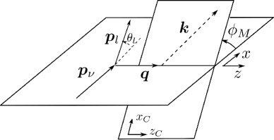
Figure 1: Momentum variables and scattering angles for a neutrino-induced single meson production reaction.

We express the hadron tensor for a two-body meson-baryon ($MB$) final state, $\nu(p_{\nu})+N(p_{N})\rightarrow l(p_{l})+M(k)+B(p)$, in terms of the matrix element of the hadronic current in the center-of-mass frame of the hadronic system (hCM). This expression is useful for working with reaction models in which the matrix elements are most easily calculated in the hCM. Also, the out-of-plane angle of the meson ($\phi_{M}$; see Fig. 1) explicitly appears in the cross section formula. We choose a coordinate system such that the $xz$-plane coincides with the lepton scattering plane, and the $z$-axis is along the momentum transfer $\bm{q}$. Regarding the coordinate system in the hCM, the meson is scattered in the $x_{C}z_{C}$-plane and the direction of the $z_{C}$-axis is chosen along $\bm{q}$. The angle between the lepton and hadron reaction planes is denoted by $\phi_{M}$, and is shown along with our coordinate system in Fig. 1. The hadron tensor for a two-body meson-baryon final state is given as

$$W^{{\rm Y},N\to MB}_{\mu\nu} = \frac{(2\pi)^{3}}{2}\sum_{s_{N}^{z},s_{B}^{z}}\int d\Omega_{M}^{*}\Lambda_{\mu}^{\ \lambda}\Lambda_{\nu}^{\ \sigma}\frac{|{\bm{k}}^{*}|E_{M}(k^{*})E_{B}(p^{*})E_{N}(p_{N}^{*})}{Wm_{N}}$$ (10)

$$\times \langle MB^{(-)}|J^{\rm Y}_{\lambda}(0)|N\rangle_{\rm hCM}\langle MB^{(-)}|J^{\rm Y}_{\sigma}(0)|N\rangle^{*}_{\rm hCM}\ .$$

Here the matrix element of the hadron current is evaluated in hCM. The initial nucleon state in hCM is $|N\rangle=|N(p_{N}^{*},s_{N}^{z},t_{N}^{z})\rangle$, while the final meson-baryon state in hCM, $|MB\rangle=|M(k^{*},t^{z}_{M})B(p^{*},s_{B}^{z},t_{B}^{z})\rangle$, has the momentum $k^{*}$ ($p^{*}$), the isospin $z$-components $t_{M}^{z}$ ($t_{B}^{z}$), and the spin $z$-component 0 ($s_{B}^{z}$) for the meson (baryon). Here we assume the meson is a pseudo-scalar particle. The momenta with the asterisk ($*$) are those in the hCM. Therefore $\bm{p}^{*}=-\bm{k}^{*}$ and $\bm{p}_{N}^{*}=-\bm{q}^{*}$. The quantity $W=\sqrt{(q+p_{N})^{2}}$ is the invariant mass of the hadronic system. We have also introduced the Lorentz transformation matrix, $\Lambda^{\ \mu}_{\nu}$, that transforms a vector in hCM to that in the laboratory frame. Nonzero elements of $\Lambda^{\ \mu}_{\nu}$ are explicitly given as

$$\Lambda^{\ 1}_{1}=\Lambda^{\ 2}_{2}=\cos\phi_{M},\ \Lambda^{\ 2}_{1}=-\Lambda^{\ 1}_{2}=-\sin\phi_{M},\ \Lambda^{\ 0}_{0}=\Lambda^{\ 3}_{3}=\frac{m_{N}+\omega}{W},\ \Lambda^{\ 0}_{3}=\Lambda^{\ 3}_{0}=-\frac{|\bm{q}|}{W}.$$

For a two-pion production, $\nu(p_{\nu})+N(p_{N})\rightarrow l(p_{l})+\pi(p_{1})+\pi(p_{2})+N(p_{N^{\prime}})$, a formal expression of the hadron tensor is given as

$$W^{{\rm Y},N\to\pi\pi N}_{\mu\nu} = {\cal B}_{\pi\pi}\frac{(2\pi)^{3}}{2}\sum_{s_{N}^{z},s_{N^{\prime}}^{z}}\int d\bm{p}_{1}d\bm{p}_{2}d\bm{p}_{N^{\prime}}\delta^{(4)}(q+p_{N}-p_{1}-p_{2}-p_{N^{\prime}})\frac{E_{N}(p_{N})}{m_{N}}$$ (12)

$$\times\langle\pi\pi N^{(-)}|J^{\rm Y}_{\mu}(0)|N\rangle\langle\pi\pi N^{(-)}|J^{\rm Y}_{\nu}(0)|N\rangle^{*}\ ,$$

where $|\pi\pi N\rangle=|\pi(p_{1},t_{1}^{z})\pi(p_{2},t_{2}^{z})N(p_{N^{\prime}},s_{N^{\prime}}^{z},t_{N^{\prime}}^{z})\rangle$ is the $\pi\pi N$ final state. The isospin states of the pions and the spin-isospin states of the final nucleon are denoted as $t_{1}^{z},t_{2}^{z}$ and $s_{N^{\prime}}^{z},t_{N^{\prime}}^{z}$, respectively. For identical pions, we need a symmetry factor, ${\cal B}_{\pi\pi}^{-1}=1+\delta_{t_{1}^{z},t_{2}^{z}}$. An explicit formula of the hadron tensor for the two-pion final state in our reaction model will be given in the next section.

Here we also introduce the inclusive cross section in which all the final hadronic states are integrated over. In the vanishing lepton mass limit, the inclusive cross section is given in terms of three structure functions, $W^{\rm Y}_{i}(W,Q^{2})$ ($i$=1,2,3; ${\rm Y}$=CC$\nu$, CC$\bar{\nu}$, NC):

$$\frac{d^{3}\sigma_{\nu N\to lX}}{dE_{l}d\Omega_{l}}=\frac{G^{2}_{F}C_{\rm Y}}{2\pi^{2}}E_{l}^{2}[2W^{\rm Y}_{1}\sin^{2}\frac{\theta_{l}}{2}+W^{\rm Y}_{2}\cos^{2}\frac{\theta_{l}}{2}\pm W^{\rm Y}_{3}\frac{E_{\nu}+E_{l}}{m_{N}}\sin^{2}\frac{\theta_{l}}{2}]\,,$$ (13)

where $C_{\rm Y}$ has been introduced in Eq. (7); the $+$ ($-$) sign in front of $W^{\rm Y}_{3}$ is for neutrino (anti-neutrino) reactions, and $\theta_{l}$ is the lepton scattering angle. The structure functions can be written with the inclusive hadron tensor evaluated in hCM and with $Q^{2}=-q^{2}$ as follows:

$$W^{\rm Y}_{1} = {1\over 2}\left(W^{\rm Y}_{xx}+W^{\rm Y}_{yy}\right)\ ,$$ (14)

$$W^{\rm Y}_{2} = {Q^{2}\over|\bm{q}|^{2}}\left(W^{\rm Y}_{1}+{Q^{2}\over|\bm{q}^{*}|^{2}}\left\{W^{\rm Y}_{00}+\left({\omega^{*}\over Q^{2}}\right)^{2}W^{\rm Y}_{\mu\nu}q^{*\mu}q^{*\nu}+2{\omega^{*}\over Q^{2}}{\rm Re}\left[W^{\rm Y}_{0\mu}\right]q^{*\mu}\right\}\right)\ ,$$ (15)

$$W^{\rm Y}_{3} = -{2m_{N}\over|\bm{q}|}{\rm Im}[W^{\rm Y}_{xy}]\ ,$$ (16)

and the dimensionless structure functions are conventionally defined by

$$F^{\rm Y}_{1} = m_{N}W^{\rm Y}_{1}\ ,\quad F^{\rm Y}_{2}=\omega W^{\rm Y}_{2}\ ,\quad F^{\rm Y}_{3}=\omega W^{\rm Y}_{3}\ .$$ (17)

The inclusive cross section within our DCC model is the sum of the two-body and three-body final states:

$$\frac{d^{3}\sigma_{\nu N\to lX}}{dE_{l}d\Omega_{l}}=\sum_{MB}\frac{d^{3}\sigma_{\nu N\to lMB}}{dE_{l}d\Omega_{l}}+\sum_{\pi\pi N}{d^{3}\sigma_{\nu N\to l\pi\pi N}\over dE_{l}d\Omega_{l}}\ ,$$ (18)

where the summation of $MB$ ($\pi\pi N$) runs over all charge states of $\pi N,\eta N,K\Lambda,K\Sigma$ ($\pi\pi N$).

Finally, we give the differential cross section with respect to $W$ and $Q^{2}$ for our later purpose:

$$\frac{d^{2}\sigma_{\nu N\to lf}}{dWdQ^{2}}={2\pi W\over 2m_{N}|\bm{p}_{\nu}||\bm{p}_{l}|}\frac{d^{3}\sigma_{\nu N\to lf}}{dE_{l}d\Omega_{l}}\ .$$ (19)

III Hadronic current in Dynamical Coupled-Channels Model

III.1 Overview of Dynamical Coupled-Channels Model

Here we present a brief and overall description of the DCC reaction model msl07 , which is followed by a more concrete and practical formulae in the next subsections. We start with an effective Hamiltonian for the meson-baryon system:

$$H = H_{0}+v+\Gamma\ .$$ (20)

The Fock space of the model consists of meson-baryon states ($\pi N,\eta N,K\Lambda,K\Sigma$ and $\pi\pi N$ states) and ’bare’ excited states ($N^{*},\Delta,\rho,\sigma$). Here the bare $N^{*}$ state represents a quark core component of the nucleon resonance; it is dressed by the meson cloud to form the resonance. We also include $\pi\Delta,\rho N$ and $\sigma N$ states as doorway states of the $\pi\pi N$ state. The symbol $H_{0}$ is the free Hamiltonian of the particles, and $v$ is non-resonant interactions among the two-body meson-baryon states and $\pi\pi$ states. The non-resonant interactions are based on the $s,t,u$-channel hadron-exchange mechanisms. $\Gamma$ represents transitions between bare excited states and two-body states such as $\Delta\leftrightarrow\pi N$. The scattering amplitude ($T$-matrix element) is obtained by solving the Lippmann-Schwinger equation as explained in detail in Ref. msl07 ; the Lippmann-Schwinger equation can be represented diagrammatically as shown in Fig. 2. The two-body scattering $T$-matrix for 7 channels $\alpha\rightarrow\beta$ ($\alpha,\beta=\pi N,\eta N,K\Lambda,K\Sigma,\pi\Delta,\rho N,\sigma N$) is given by the sum of non-resonant and resonant $T$-matrix as

$$\langle\beta|T^{(\pm)}(W)|\alpha\rangle = \langle\beta|t^{(\pm)}_{\rm non-res}(W)|\alpha\rangle+\langle\beta|t^{(\pm)}_{\rm res}(W)|\alpha\rangle\ ,$$ (21)

where the superscript $+(-)$ indicates the outgoing (incoming) boundary condition. Each term of the above equation corresponds to the diagram in Fig. 2 in the same ordering. The non-resonant $T$-matrix is obtained by solving the Lippmann-Schwinger equation,

$$\langle\beta|t^{(\pm)}_{\rm non-res}(W)|\alpha\rangle = \langle\beta|[V^{(\pm)}(W)+V^{(\pm)}(W)G^{(\pm)}_{MB}(W)t^{(\pm)}_{\rm non-res}(W)]|\alpha\rangle\ ,$$ (22)

where $G^{(\pm)}_{MB}(W)$ is Green function of a meson-baryon state; this is the free Green function for the stable channels such as $MB=\pi N,\eta N,K\Lambda,K\Sigma$, while for the unstable $MB=\pi\Delta,\rho N,\sigma N$ channels the Green function contains the self-energy to account for the decay into the $\pi\pi N$ channel.

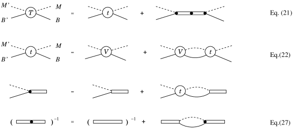
Figure 2: (Color online) Diagrammatic representation of the Lippmann-Schwinger equation. The corresponding equation numbers in the text are indicated on the right. The symbols $T$, $t$, and $V$ in the figures correspond to $T^{(\pm)}(W)$ and $t^{(\pm)}_{\rm non-res}(W)$ in Eq. (21), and $V^{(\pm)}(W)$ in Eq. (23), respectively. The third line represents the dressed $N^{*}$ decay vertex, $\langle\chi^{(-)}|\Gamma|N^{*}\rangle$, contained in Eq. (26). The double lines represent $N^{*}$-propagators and the fourth line corresponds to Eq. (27).

The effective two-body interaction is the sum of the interaction $v$ and the contribution of particle exchange ’Z-diagram’ that contains the $\pi\pi N$ intermediate state as

$$V^{(\pm)}(W)=v+Z^{(\pm)}(W).$$ (23)

Introducing a wave operator $\Omega^{(+/-)}$ and a scattering state $\chi^{(+/-)}$ for outgoing/incoming boundary condition as

$$\Omega^{(\pm)}(W) = 1+G^{(\pm)}_{MB}(W)t^{(\pm)}_{\rm non-res}(W)\ ,$$ (24)

$$|\chi_{\alpha}^{(\pm)}\rangle = \Omega^{(\pm)}|\alpha\rangle\ ,$$ (25)

the resonant $T$-matrix is given by

$$\langle\beta|t^{(+)}_{\rm res}(W)|\alpha\rangle = \sum_{m,n}\langle\chi_{\beta}^{(-)}|\Gamma|N^{*}_{m}\rangle[D(W)]_{m,n}\langle N^{*}_{n}|\Gamma|\chi_{\alpha}^{(+)}\rangle\ ,$$ (26)

where the summation is taken over all the considered bare $N^{*}$ and $\Delta$ states labelled by the indices, $m$ and $n$. The $N^{*}$ propagator is denoted by $[D(W)]_{m,n}$, and it can have nonzero off-diagonal elements through the rescattering as

$$[D^{-1}(W)]_{m,n} = (W-m_{m}^{0})\delta_{m,n}+\langle N^{*}_{m}|\Gamma\Omega^{(+)}(W)G_{MB}^{(+)}(W)\Gamma|N^{*}_{n}\rangle\ ,$$ (27)

for $N^{*}_{m}$ and $N^{*}_{n}$ belonging to the same partial wave. In the above equation, $m_{m}^{0}$ is the bare mass for $N^{*}_{m}$. All the parameters appearing in the strong interaction Hamiltonian have already been determined in our previous analysis knls13 .

Electroweak meson production reactions on a nucleon ($\gamma+N\rightarrow X$, $e+N\rightarrow e^{\prime}+X$ and $\nu+N\rightarrow l+X$) within the DCC reaction model are described in terms of the matrix element of the hadron current $J^{\mu}$ which is, for example, the current in Eq. (3) for the CC neutrino reaction. In the DCC model, the hadron current consists of non-resonant meson-production current and bare resonant current as

$$J^{\mu}=j^{\mu}_{\rm non-res}+j^{\mu}_{\rm res}\ ,$$ (28)

where we have suppressed the label “Y”(=CC, NC) for simplicity, and we will do the same to the symbols $J^{\mu}$ and $j^{\mu}$ in the rest of this section. The currents, $j^{\mu}_{\rm non-res}$ and $j^{\mu}_{\rm res}$, are the electroweak counterparts of $v$ and $\Gamma$ in the strong interaction Hamiltonian. Meson-baryon states produced by the current experience multiple rescattering to form final states. These scattering processes are described by $T$ matrix elements [Eq. (21)] that satisfy the unitarity condition. Thus the matrix element of the hadron current between nucleon and meson-baryon scattering state $\langle\alpha^{(-)}|$ is given as

$$\langle\alpha^{(-)}|J^{\mu}|N\rangle = \langle\chi_{\alpha}^{(-)}|j^{\mu}_{\rm non-res}|N\rangle$$ (29)

$$+ \sum_{m,n}\langle\chi_{\alpha}^{(-)}|\Gamma|N^{*}_{m}\rangle[D(W)]_{m,n}\langle N^{*}_{n}|j^{\mu}_{\rm res}+\Gamma\Omega^{(+)}(W)G^{(\pm)}_{MB}(W)j^{\mu}_{\rm non-res}|N\rangle\ ,$$

where the first term on the r.h.s. is purely from non-resonant dynamics while the second term is due to excitations of nucleon resonances. This matrix element is the input to calculate the hadron tensor in Eq. (9). A more definite expression of the matrix element will be given in the next subsection. We note that not only the on-shell matrix elements but also their off-energy-shell behavior are obtained in the DCC model.

Finally, a matrix element of the hadron current that contributes to the $\pi\pi N$ final state is given within the DCC model used in this work as follows:

$$\langle\pi\pi N^{(-)}|J^{\mu}|N\rangle = \langle\pi N|\Gamma|N\rangle G_{\pi N}^{(+)}(W)\langle\pi N^{(-)}|J^{\mu}|N\rangle$$ (30)

$$+ \langle\pi N|\Gamma|\Delta\rangle G_{\pi\Delta}^{(+)}(W)\langle\pi\Delta^{(-)}|J^{\mu}|N\rangle$$

$$+ \langle\pi\pi|\Gamma|\rho\rangle G_{\rho N}^{(+)}(W)\langle\rho N^{(-)}|J^{\mu}|N\rangle$$

$$+ \langle\pi\pi|\Gamma|\sigma\rangle G_{\sigma N}^{(+)}(W)\langle\sigma N^{(-)}|J^{\mu}|N\rangle\ ,$$

where $\langle MB^{(-)}|$ contains the hadronic rescattering as has been defined in Eqs. (24), (25) and (29), while $\langle\pi N|$ and $\langle\pi\pi|$ are non-interacting states.

Through our previous analysis of the pion- and photon-induced meson production reactions, we have already constructed a DCC model for the strong interaction and the electromagnetic current of the proton at $Q^{2}$=0. Also, all the resonance parameters such as the masses and strong decay widths have been extracted from the DCC model knls13 . In order to extend the model to calculate neutrino-induced reaction cross sections, our main task is to develop an axial-current model for $j^{\mu}_{\rm non-res}$ and $j^{\mu}_{\rm res}$. We also need to determine the $Q^{2}$-dependence of the vector form factors associated with $N$-$N^{*}$ transitions by analyzing both electron-proton and electron-neutron reaction data.

III.2 Formulae for numerical calculations

Based on the discussion in the previous subsection, we here present formulae that are practically used in numerical calculations. Particularly, we give expressions for matrix elements of the hadron current that are directly plugged in the hadron tensor defined in Sec. II. In this subsection, all kinematical variables are those in hCM, and thus we suppress the asterisk $({}^{*})$ used in the previous section for simplicity.

Let us consider the matrix element, defined in Eq. (29), for a meson production off the nucleon induced by the hadron current $J_{\mu}$, $\langle M(\bm{k})B(-\bm{k})^{(-)}|J_{\mu}(\bm{q},Q^{2})|N(-\bm{q})\rangle$, where $MB$=$\pi N$, $\eta N$, $\pi\Delta$, $\rho N$, $\sigma N$, $K\Lambda$, $K\Sigma$. For calculating the matrix element, we find it convenience to expand the matrix element in term of the the helicity-$LSJ$ mixed representation; $L$, $S$, and $J$ are the orbital angular momentum, total spin, and total angular momentum, respectively, for the final $MB$ state. For a detailed discussion on the $LSJ$- and mixed-representations we employ, see Appendices C and D in Ref. knls13 . Thus the matrix element of the hadron current is expressed as follows:

$$\langle M(\bm{k};s_{M}s_{M}^{z}t_{M}t_{M}^{z})B(-\bm{k};s_{B}s_{B}^{z}t_{B}t_{B}^{z})^{(-)}|J(\bm{q},Q^{2})\cdot\epsilon(\lambda)|N(-\bm{q};s_{N}s_{N}^{z}t_{N}t_{N}^{z})\rangle$$ (31)

$$= \sum_{LSJIL^{z}}\sqrt{2J+1\over 4\pi}(t_{M}t_{M}^{z}t_{B}t_{B}^{z}|II^{z})(t_{J}t_{J}^{z}t_{N}t_{N}^{z}|II^{z})(s_{M}s_{M}^{z}s_{B}s_{B}^{z}|SS^{z})$$

$$\times(LL^{z}SS^{z}|Js_{N}^{z}\!+\!m(\lambda))Y_{LL^{z}}(\hat{k})\,T_{MB,JN}(\lambda;k,q;W,Q^{2})\ ,$$

where $\bm{q}$ is taken along the $z$-axis. The spin (isospin) and its $z$-component for a particle $x$ are denoted by $s_{x}$ and $s_{x}^{z}$ ($t_{x}$ and $t_{x}^{z}$), respectively; $t_{J}$ is the isospin of the hadron current. The total isospin of the final $MB$ system is denoted by $I$. The notation $(j_{1}j_{1}^{z}j_{2}j_{2}^{z}|j_{3}j_{3}^{z})$ stands for the Clebsch-Gordan coefficient. Also, we denoted the polarization of the hadron current by $\lambda=t,-1,0,1$ in the spherical basis ($t$: time component), and $\epsilon(\lambda)$ is the corresponding polarization vector; $m(\lambda)=0,-1,0,1$ are for $\lambda=t,-1,0,1$, respectively. We have introduced the matrix element in the helicity-$LSJ$ mixed representation denoted by $T_{MB,JN}(\lambda;k,q;W,Q^{2})$ in which the label $MB$ is understood to include quantum numbers such as $L,S,J$, and $I$. The matrix element on the l.h.s. of Eq. (31) is $\langle MB^{(-)}|J_{\lambda}(0)|N\rangle_{\rm hCM}$ in Eq. (10). Thus we are now left with evaluating the hadron current matrix elements in the helicity-$LSJ$ mixed representation, $T_{MB,JN}$, in order to calculate neutrino cross sections using the formulae presented in Sec. II.

Following the manner in the previous subsection, we divide the matrix element into non-resonant and resonant parts as

$$T_{MB,JN}(\lambda;k,q;W,Q^{2})=t_{MB,JN}(\lambda;k,q;W,Q^{2})+t^{R}_{MB,JN}(\lambda;k,q;W,Q^{2})\ ,$$ (32)

where $t_{MB,JN}$ is non-resonant amplitude, corresponding to the first term in Eq. (29), and is calculated by

$$t_{MB,JN}(\lambda;k,q;W,Q^{2})=v_{MB,JN}(\lambda;k,q;Q^{2})$$

$$+\sum_{M^{\prime}B^{\prime}}\int p^{2}dp\,t_{MB,M^{\prime}B^{\prime}}(k,p;W)\,G_{M^{\prime}B^{\prime}}(p;W)\,v_{M^{\prime}B^{\prime},JN}(\lambda;p,q;Q^{2}),$$ (33)

where $v_{MB,JN}$ denotes a tree-level non-resonant current matrix element, $\langle MB|j_{\rm non-res}\cdot\epsilon(\lambda)|N\rangle$ [$j_{\rm non-res}$ from Eq. (28)], projected onto the helicity-$LSJ$ mixed representation. We will specify $v_{MB,JN}$ in the following subsection. Also, $t_{MB,M^{\prime}B^{\prime}}$ is the non-resonant hadronic scattering amplitude expressed with the $LSJ$ representation, and $G_{M^{\prime}B^{\prime}}$ is a meson-baryon Green’s function. The second term in Eq. (32) is the resonant amplitude, corresponding to the second term in Eq. (29), and is given by

$$t^{R}_{MB,JN}(\lambda;k,q;W,Q^{2}) = \sum_{m,n}\bar{\Gamma}_{MB,N^{\ast}_{m}}(k;W)[D(W)]_{m,n}\bar{\Gamma}_{N^{\ast}_{n},JN}(\lambda;q;W,Q^{2}),$$ (34)

$$\bar{\Gamma}_{N^{\ast},JN}(\lambda;q;W,Q^{2}) = \Gamma_{N^{\ast},JN}(\lambda;q,Q^{2})$$

$$+ \sum_{M^{\prime}B^{\prime}}\int p^{2}dp\,\Gamma_{N^{*},M^{\prime}B^{\prime}}(p)\,G_{M^{\prime}B^{\prime}}(p,W)\,t_{M^{\prime}B^{\prime},JN}(\lambda;p,q;W,Q^{2})\ ,$$

where $\Gamma_{N^{*},JN}$ denotes a bare $N^{*}$-excitation current, $\langle N^{\ast}|j_{\rm res}\cdot\epsilon(\lambda)|N\rangle$ [$j_{\rm res}$ from Eq. (28)], for which explicit expressions are given in Appendix B (Appendix C) for the axial-current (vector-current). We have also used $\Gamma_{MB,N^{\ast}}$, $\bar{\Gamma}_{MB,N^{\ast}}$ and $D(W)$ that are bare, dressed $N^{*}\to MB$ decay amplitudes and a dressed $N^{*}$ propagator, respectively. These quantities and $t_{MB,M^{\prime}B^{\prime}}$ and $G_{MB}$ in Eq. (33) have been defined and well discussed in Sec. II A of Ref. knls13 , and we will not repeat it here.

Before closing this subsection, we derive the hadron tensor for neutrino-induced double-pion productions. Because we have specified coupled channels considered in our DCC model, we can manipulate Eq. (12) to a more definite form to be used in actual calculations. As we mentioned, $\pi\Delta,\rho N,\sigma N$ are the doorway states into the $\pi\pi N$ channel in the DCC model, and they contribute to the double pion productions as in Eq. (30). In addition, we also include a mechanism of the hadron current-induced $N\to\pi+N$ transition followed by a perturbative $N\to\pi N$ process for the double-pion productions, as in the first term of Eq. (30). In principle, different doorway state contributions shown on the r.h.s. of Eq. (30) can interfere with each other. Also, even within the $\pi\Delta$ doorway state contribution, there is still an interference between diagrams in which the final two pions are interchanged. However, we can estimate these interference contributions to be small for total cross sections and $d^{2}\sigma/dWdQ^{2}$ because of the fact that the Z-diagrams in our currently used DCC model give rather small contributions to the $\pi N$ scattering knls13 . We note however that the interference could be more important for differential cross sections with respect to the pion emission angles, which we will not calculate in this work, as has been seen in Ref. msl07 . Thus we ignore the interference to derive a simpler hadron tensor for the double-pion production. For example, the contribution from the $\pi\Delta$ doorway state to $\pi_{1}\pi_{2}N$ production is given by

$$W^{{\rm Y},N\to\pi\Delta\to\pi_{1}\pi_{2}N}_{\mu\nu} = {\cal B}_{\pi\pi}\sum_{\{ab\}}\int^{W-m_{\pi}}_{m_{\pi}+m_{N}}dM_{\pi_{b}N}\frac{1}{2\pi}\frac{M_{\pi_{b}N}}{E_{\Delta}(k)}\frac{(t_{\pi_{b}}t^{z}_{\pi_{b}}t_{N}t^{z}_{N}|t_{\Delta}t^{z}_{\pi_{b}}+t^{z}_{N})^{2}\Gamma_{\Delta\to\pi_{b}N}(k;W)}{|W-E_{\pi_{a}}(k)-E_{\Delta}(k)-\Sigma_{\Delta\pi_{a}}(k;W)|^{2}}$$ (36)

$$\times W_{\mu\nu}^{{\rm Y},N\to\pi_{a}\Delta},$$

where $M_{\pi_{b}N}$ is the invariant mass of the $\pi_{b}N$ pair from the $\Delta$-decay, and $k$ is given by the relation, $W=E_{\pi_{a}}(k)+\sqrt{M_{\pi_{b}N}^{2}+k^{2}}$; $\Sigma_{\pi_{a}\Delta}(k;W)$ is the self-energy of the $\pi_{a}\Delta$ Green’s function as summarized in Appendix A of Ref. knls13 ; $\Gamma_{\Delta\to\pi_{b}N}(k;W)=-2\mathrm{Im}[\Sigma_{\pi_{a}\Delta}(k;W)]$; $(t_{\pi_{b}}t^{z}_{\pi_{b}}t_{N}t^{z}_{N}|t_{\Delta}t^{z}_{\pi_{b}}+t^{z}_{N})^{2}\Gamma_{\Delta\to\pi_{b}N}(k;W)$ gives the partial width of $\Delta$ into a given isospin state of $\pi_{b}N$; $\sum_{\{ab\}}$ indicates the sum over the permutations of the two pions, i.e., ${\{ab\}}={\{12\}},{\{21\}}$; the symmetry factor ${\cal B}_{\pi\pi}$ has been defined below Eq. (12). The quasi two-body hadron tensor, $W_{\mu\nu}^{{\rm Y},N\to\pi_{a}\Delta}$, is calculated using Eq. (10) similarly to the other stable two-body channels. A difference from the stable channel case is that $k$ determined above is used instead of the on-shell momentum. The hadron tensors for the double-pion productions due to the other doorway states can be derived in a similar manner.

III.3 Matrix elements of non-resonant currents

We here specify matrix elements of non-resonant current, $j^{\mu}_{\rm non-res}$ in Eq. (28), for meson productions. The matrix elements are projected onto the helicity-$LSJ$ state and plugged into $v_{MB,JN}$ in Eq. (33). As in Eqs. (3) and (5), the current consists of the vector and axial currents. Matrix elements of the non-resonant vector current at $Q^{2}=0$ have been fixed through the previous analysis of photon-induced meson-production data, and explicit expressions are given in Appendix D of Ref. knls13 . We also need to fix the $Q^{2}$-dependence of the matrix elements to study electron- and neutrino-induced reactions, and we use the parametrization given in Appendix A of Ref. nl1990 .

Regarding the axial current, we take advantage of the fact that most of our $\pi N\to MB$ potentials are derived from a chiral Lagrangian. Thus, we basically follow the way how the axial current is introduced in the chiral Lagrangian: an external axial current ($a^{\mu}_{\rm ext}$) enters into the chiral Lagrangian in combination with the pion field as $\partial^{\mu}\pi+f_{\pi}a^{\mu}_{\rm ext}$ where $f_{\pi}$ is the pion decay constant. Therefore, matrix elements of the hadronic axial current are obtained from those of $\pi N\rightarrow MB$ by a replacement $k^{\mu}\to if_{\pi}\epsilon^{\mu}(\lambda)$, where $k^{\mu}$ is the four-momentum of the incoming pion and $\epsilon^{\mu}(\lambda)$ is the polarization vector for $a^{\mu}_{\rm ext}$ with a polarization $\lambda$. We apply this replacement to the $\pi N\rightarrow MB$ potentials of the DCC model presented in Appendix C of Ref. knls13 . The tree-level axial current matrix elements constructed in this way are the non pion-pole part of the axial currents, $\langle MB|A^{i}_{\rm NP,tree}\cdot\epsilon(\lambda)|N\rangle$ ($i$: isospin component), and their expressions are presented in Appendix A of this paper. By construction, $A^{i,\mu}_{\rm NP,tree}$ and the meson-baryon potential $v$ satisfy the PCAC relation at $Q^{2}=-m^{2}_{\pi}$ yamagishi :

$$\langle MB|q\cdot A^{i}_{\rm NP,tree}|N\rangle=if_{\pi}\langle MB|v|\pi^{i}N\rangle\ .$$ (37)

The axial-current matrix element $A^{i,\mu}$ in Eqs. (3) and (5) is related to the non pion-pole part, $A^{i,\mu}_{\rm NP}$, by

$$A^{i,\mu}=A^{i,\mu}_{\rm NP}+q^{\mu}{1\over Q^{2}+m^{2}_{\pi}}q\cdot A^{i}_{\rm NP}\ ,$$ (38)

where the second term is the pion-pole term. In the DCC model of Ref. knls13 , we needed to introduce some meson-baryon potentials that are not from a chiral Lagrangian in order to fit a large amount of $\pi$-induced reaction data. Although we cannot apply the above replacement to derive the axial currents for those potentials, we can still add the corresponding axial currents to maintain the PCAC relation, as given in Eqs. (61), (62), (65), and (101).

The $Q^{2}$-dependence of the axial-coupling of the nucleon has been studied through data analyses of quasi-elastic neutrino scattering and single pion electroproduction near threshold. In the analyses, the axial mass ($M_{A}$) of the dipole form factor $F_{A}(Q^{2})=1/(1+Q^{2}/M^{2}_{A})^{2}$, has been determined to be $M_{A}$ = $1.026\pm 0.021$ GeV axial-mass . We employ this axial form factor, and assume that all non-resonant axial current amplitudes have the same $Q^{2}$-dependence.

III.4 Matrix elements of $N^{*}$-excitation currents

Here, we specify the last piece of the DCC model, $\Gamma_{N^{\ast},JN}(\lambda;q,Q^{2})$ in Eq. (LABEL:eq:nstargn).

III.4.1 Vector current

The hadronic vector current contributes to the neutrino-induced reactions in the finite $Q^{2}$ region. In Ref. knls13 , we have done a combined analysis of $\pi N,\gamma p\to\pi N,\eta N,K\Lambda,K\Sigma$ reaction data, and fixed matrix elements of the vector current at $Q^{2}=0$ for the proton target. The bare $N$-$N^{*}$-transition matrix elements induced by the vector current are parametrized and presented in Appendix C. What we need to do is to extend the matrix elements of the vector current of Ref. knls13 to the finite $Q^{2}$ region for application to the neutrino reactions. More concretely, we determine $Q^{2}$-dependence of $\tilde{M}_{l\pm}^{NN^{*}}(Q^{2})$, $\tilde{E}_{l\pm}^{NN^{*}}(Q^{2})$, $\tilde{S}_{l\pm}^{NN^{*}}(Q^{2})$, $x_{A_{3/2}}(Q^{2})$ and $x_{A_{1/2}}(Q^{2})$, which we collectively denote by $F^{V}_{NN^{*}}(Q^{2})$, for the proton and the neutron. (See Appendix C for the definition of the symbols.) This can be done by analyzing data for electron-induced reactions on the proton and the neutron, and analysis results will be presented in Sec. IV. Then we separate the vector form factors for $N^{*}$ of $I=1/2$ ($I$: isospin) into isovector and isoscalar parts as discussed in Appendix C. Regarding $N^{*}$ of $I=3/2$ for which only the isovector current contributes, we can determine the vector form factors by analyzing the proton-target data.

III.4.2 Axial current

Because of rather scarce neutrino reaction data, it is difficult to determine $N$-$N^{*}$ transition matrix elements induced by the axial-current. This is in sharp contrast with the situation for the vector form factors that are well determined by a large amount of electromagnetic reaction data. Thus, we need to take a different path to fix the axial form factors. The conventional practice is to write down a $N$-$N^{*}$ transition matrix element induced by the axial-current in a general form with three or four form factors. Then the PCAC relation, $\langle N^{*}|q\cdot A^{i}_{\rm NP}|N\rangle=if_{\pi}\langle N^{*}|\Gamma|\pi^{i}N\rangle$, is invoked to relate the presumably most important axial form factor at $Q^{2}=-m^{2}_{\pi}$ to the corresponding $\pi NN^{*}$ coupling. The other form factors are ignored except for the pion pole term. We then assume $A^{i,\mu}_{\rm NP}(Q^{2}=-m^{2}_{\pi})\sim A^{i,\mu}_{\rm NP}(Q^{2}=0)$. In the present work, we consider the axial currents for bare $N^{*}$ of the spin-parity $1/2^{\pm}$, $3/2^{\pm}$, $5/2^{\pm}$ and $7/2^{\pm}$, and determine their axial form factors at $Q^{2}=0$ using the above procedure. For more detail including explicit formulae, see Appendix B. It is even more difficult to determine the $Q^{2}$-dependence of the axial couplings to $N$-$N^{*}$ transitions because of the limited amount of data. Thus we assume that the $Q^{2}$-dependence of the axial form factors is the same as that used for the non-resonant axial-current amplitudes, i.e., the conventional dipole form factor with $M_{A}$=1.02 GeV. When necessary, we can adjust the axial mass for an axial $N$-$N^{*}$ coupling to fit available data.

It is worth emphasizing that a great advantage of our approach over the existing models is that relative phases between resonant and non-resonant amplitudes are made under control within the DCC model. This is possible in our approach by constructing the axial-current amplitudes and $\pi N$ interactions consistently with the requirement of the PCAC relation. As we will see, the resonant and non-resonant contributions to the neutrino reactions are sometimes comparable in magnitude and, in such a circumstance, it is essential to have a well-controlled relative phases between them to correctly describe the neutrino reactions. We also note that our DCC $\pi N$ model, on which the axial-current is based, has been extensively tested by data in Ref. knls13 .

IV Analysis of electron-induced reaction data

In this section, we analyze data for electron-induced reactions off the proton and neutron targets to determine the $Q^{2}$ dependence of $F^{V}_{NN^{*}}(Q^{2})$, namely $\tilde{M}^{NN^{*}}_{l\pm}(Q^{2})$, $\tilde{E}^{NN^{*}}_{l\pm}(Q^{2})$, $\tilde{S}^{NN^{*}}_{l\pm}(Q^{2})$, $x_{A_{3/2}}(Q^{2})$, and $x_{A_{3/2}}(Q^{2})$, which are our model parameters associated with the vector transition form factors and are defined in Appendix C. As explained in Sec. III.4.1, for the isospin $I=1/2$ nucleon resonances, the analysis of electron-induced reactions on both the proton- and neutron-targets is required to decompose the electromagnetic transition form factors into the isovector and isoscalar parts. This decomposition is necessary for calculating the CC and NC reactions. Regarding $I=3/2$ nucleon resonances, on the other hand, we determine the $F^{V}_{NN^{*}}(Q^{2})$ by analyzing only proton-target reactions data. The data we analyze span the kinematical region of $W\leq$ 2 GeV and $Q^{2}\leq$ 3 (GeV/$c$)² that is also shared by neutrino reactions for $E_{\nu}\leq$ 2 GeV. Meanwhile, it is a challenge for the DCC model to predict cross sections of various final hadron states in the finite $Q^{2}$ region by adjusting only the ’bare’ $N$-$N^{*}$ transition form factors. Thus the analysis of the electron-induced reaction data also serves as a testing ground for the soundness of the DCC model.

IV.1 Electron-proton reactions

Among data for electron-proton reactions in the resonance region, those for the single pion electroproductions are the most abundant over a wide range of $W$ and $Q^{2}$. Therefore, these are the most useful to determine the $Q^{2}$ dependence of the $p$-$N^{*}$ transition form factors. The cross sections for $p(e,e^{\prime}\pi^{0})p$ and $p(e,e^{\prime}\pi^{+})n$ have different sensitivities to resonances of different isospin state ($1/2$ or $3/2$). The angular distribution of the pion is useful to disentangle the spin-parity of the resonances. Based on the one-photon exchange approximation, a standard formula of the angular distribution for the single pion electroproduction can be expressed in terms of virtual photon cross sections $\displaystyle{d\sigma_{\beta}(Q^{2},W,\cos\theta_{\pi}^{*})}/{d\Omega_{\pi}^{*}}$ ($\beta=T,L,LT,TT,LT^{\prime}$) for the $\gamma^{*}N\to\pi N$ process in the hCM as,

$$\frac{d^{5}\sigma_{ep\rightarrow e^{\prime}\pi N}}{dE_{e^{\prime}}d\Omega_{e^{\prime}}d\Omega_{\pi}^{*}} = \Gamma_{\gamma}\left[\frac{d\sigma_{T}}{d\Omega_{\pi}^{*}}+\epsilon\frac{d\sigma_{L}}{d\Omega_{\pi}^{*}}+\sqrt{2\epsilon(1+\epsilon)}\frac{d\sigma_{LT}}{d\Omega_{\pi}^{*}}\cos\phi_{\pi}^{\ast}\right.$$ (39)

$$\left.+\epsilon\frac{d\sigma_{TT}}{d\Omega_{\pi}^{*}}\cos 2\phi_{\pi}^{\ast}+h_{e}\sqrt{2\epsilon(1-\epsilon)}\frac{d\sigma_{LT^{\prime}}}{d\Omega_{\pi}^{*}}\sin\phi_{\pi}^{\ast}\right]\ ,$$

where

$$\displaystyle\Gamma_{\gamma}=\frac{\alpha}{2\pi^{2}Q^{2}}\frac{E_{e^{\prime}}}{E_{e}}\frac{q_{\gamma}}{1-\epsilon}\ ,$$ (40)

and $q_{\gamma}=(W^{2}-m_{N}^{2})/2m_{N}$, $\epsilon=[1+2(q_{\gamma}^{2}/Q^{2})\tan^{2}(\theta_{e^{\prime}}/2)]^{-1}$, the scattering angle of electron $\theta_{e^{\prime}}$, the magnitude of the virtual photon three momentum $q_{\gamma}$, and the incident (outgoing) electron energy $E_{e}$ ($E_{e^{\prime}}$) in the laboratory frame; $h_{e}$ is the helicity of the incoming electron; $\phi_{\pi}^{\ast}$ ($\phi_{M}$ in Fig. 1) is the angle between the $\pi$-$N$ plane and the plane of the incoming and outgoing electrons. The formulae for calculating $d\sigma_{\beta}/d\Omega_{\pi}^{*}$ from the amplitudes defined by Eq. (32) are given in Ref. sl09 .

The CLAS Collaboration has collected data eepi-joo-prl ; eepi-joo-prc ; eepi-egiyan-prc ; clas-park ; clas-park2 ; clas-ungaro ; clas-smith ; clas-Aznauryan for the single pion electroproduction off the proton in the kinematical region of our interest, as shown in Fig. 3. Then they have extracted from the data the virtual photon cross sections introduced above joo-smith , i.e., $d\sigma_{T}/d\Omega_{\pi}^{*}+\epsilon d\sigma_{L}/d\Omega_{\pi}^{*}$, $d\sigma_{LT}/d\Omega_{\pi}^{*}$, $d\sigma_{TT}/d\Omega_{\pi}^{*}$, and $d\sigma_{LT^{\prime}}/d\Omega_{\pi}^{*}$. We fit these virtual photon cross sections to determine the $Q^{2}$ dependence of the $p$-$N^{*}$ transition form factors.

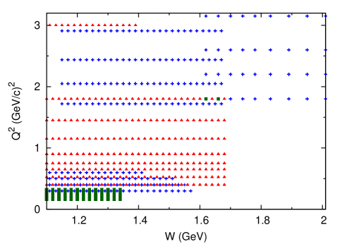
Figure 3: (Color online) Kinematical region covered by available single pion electroproduction data from the CLAS Collaboration eepi-joo-prl ; eepi-joo-prc ; eepi-egiyan-prc ; clas-park ; clas-park2 ; clas-ungaro ; clas-smith ; clas-Aznauryan . The red triangle [blue cross] points indicate the kinematical points where data for $p(e,e^{\prime}\pi^{0})p$ [$p(e,e^{\prime}\pi^{+})n$] are available. At the green square points, both $p(e,e^{\prime}\pi^{0})p$ and $p(e,e^{\prime}\pi^{+})n$ data are available.

As seen in Fig. 3, the single pion electroproduction data occupy a substantial portion of the relevant kinematical region of $W$ and $Q^{2}$. In some kinematical region, however, we still need more data to fix the vector form factors. In particular, data are missing for the $W\ \raise 1.29167pt\hbox{$>$\kern-7.5pt\lower 4.30554pt\hbox{$\sim$}}\ 1.4$ GeV and low-$Q^{2}$ region, and the $W\ \raise 1.29167pt\hbox{$>$\kern-7.5pt\lower 4.30554pt\hbox{$\sim$}}\ 1.7$ GeV and $Q^{2}\ \raise 1.29167pt\hbox{$<$\kern-7.5pt\lower 4.30554pt\hbox{$\sim$}}\ 2$ (GeV/$c$)². In those kinematical region, we fit the inclusive structure functions from an empirical model due to Christy and Bosted christy . The inclusive cross section is defined as

$$\frac{d^{3}\sigma_{ep\rightarrow e^{\prime}X}}{dE_{e^{\prime}}d\Omega_{e^{\prime}}} = \Gamma_{\gamma}\left[\sigma_{T}(W,Q^{2})+\epsilon\sigma_{L}(W,Q^{2})\right]\ ,$$ (41)

and the proton structure functions $W_{i}^{\rm em}$ [cf. Eqs. (14) and (15)] are related to the transverse and longitudinal cross sections as

$$W_{1}^{\rm em} = \frac{q_{\gamma}}{4\pi^{2}\alpha}\sigma_{T}(W,Q^{2})\ ,$$

$$W_{2}^{\rm em} = \frac{q_{\gamma}}{4\pi^{2}\alpha}\frac{Q^{2}}{Q^{2}+\omega^{2}}[\sigma_{T}(W,Q^{2})+\sigma_{L}(W,Q^{2})]\ .$$ (42)

We remark that an analysis of electron reaction data is also interesting in the context of studying the structure of nucleon resonances, and we are conducting a fuller and more dedicated analysis of electroproduction data to be reported elsewhere knls-e .

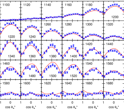
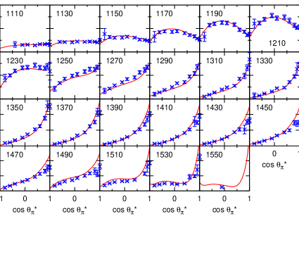
Figure 4: (Color online) The virtual photon cross section $d\sigma_{T}/d\Omega^{*}_{\pi}+\epsilon\,d\sigma_{L}/d\Omega^{*}_{\pi}$ ($\mu$b/sr) at $Q^{2}$=0.40 (GeV/$c$)² for $p(e,e^{\prime}\pi^{0})p$ (left) and $p(e,e^{\prime}\pi^{+})n$ (right) from the DCC model. The number in each panel indicates $W$ (MeV). The data are from Ref. eepi-joo-prl for $p(e,e^{\prime}\pi^{0})p$, and Ref. eepi-egiyan-prc for $p(e,e^{\prime}\pi^{+})n$.

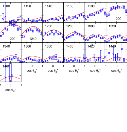
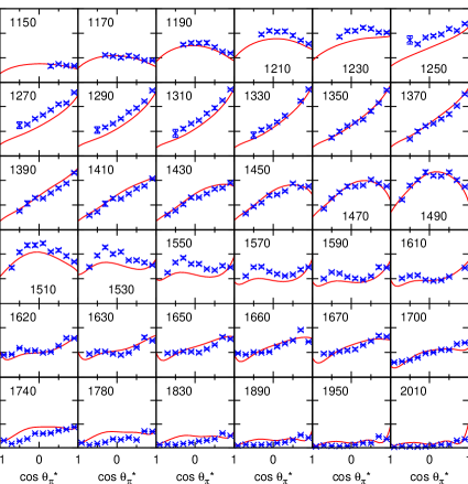
Figure 5: (Color online) The virtual photon cross section $d\sigma_{T}/d\Omega^{*}_{\pi}+\epsilon\,d\sigma_{L}/d\Omega^{*}_{\pi}$ ($\mu$b/sr) at $Q^{2}$=1.76 (GeV/$c$)². The data are in the range, $1.72\leq Q^{2}\leq$1.80 (GeV/$c$)², and are from Ref. eepi-joo-prl for $p(e,e^{\prime}\pi^{0})p$, and Refs. clas-park ; clas-park2 for $p(e,e^{\prime}\pi^{+})n$. The other features are the same as those in Fig. 4.

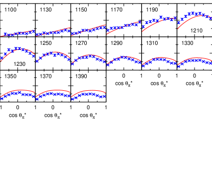
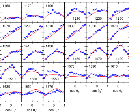
Figure 6: (Color online) The virtual photon cross section $d\sigma_{T}/d\Omega^{*}_{\pi}+\epsilon\,d\sigma_{L}/d\Omega^{*}_{\pi}$ ($\mu$b/sr) at $Q^{2}$=2.95 (GeV/$c$)². The data are in the range, $2.91\leq Q^{2}\leq$3.00 (GeV/$c$)², and are from Ref. clas-ungaro for $p(e,e^{\prime}\pi^{0})p$ and Refs. clas-park ; clas-park2 for $p(e,e^{\prime}\pi^{+})n$. The other features are the same as those in Fig. 4.

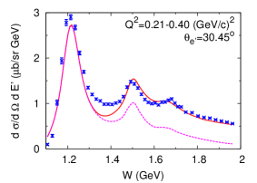
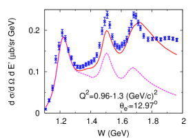
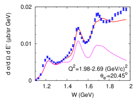
Figure 7: (Color online) Comparison of DCC-based calculation with data for inclusive electron-proton scattering at $E_{e}$=5.498 GeV. The red solid curves are for inclusive cross sections while the magenta dashed-curves are for contributions from the $\pi N$ final states. The range of $Q^{2}$ and the electron scattering angle ($\theta_{e^{\prime}}$) are indicated in each panel. The data are from Ref. E00-002 .

We have fitted $F^{V}_{pN^{*}}(Q^{2})$ to the data at several $Q^{2}$ values where the data are available. All the other parameters in the DCC model, 406 (115) parameters for hadronic ($\gamma$-$p$) interactions, are fixed as those determined by the combined analysis knls13 of $\pi N,\gamma p\to\pi N,\eta N,K\Lambda,K\Sigma$ data consisting of 22,348 data points. We have successfully tested the DCC-based vector current model with the data covering the whole kinematical region relevant to neutrino reactions of $E_{\nu}\leq 2$ GeV. Before presenting numerical results of the analysis, we take one more step as follows. In the course of the analysis, we have determined the $p$-$N^{*}$ vector form factors $F^{V}_{pN^{*}}(Q_{i}^{2})$ at particular $Q_{i}^{2}$ values where the data are available: $Q_{i}^{2}$=0, 0.16, 0.20, 0.24, 0.28, 0.30, 0.32, 0.40, 0.50, 0.525, 0.60, 0.65, 0.75, 0.90, 1.15, 1.45, 1.72, 1.80, 2.05, 2.20, 2.44, 2.60, 2.91, 3.00 (GeV/$c$)². When the model is applied to calculating neutrino cross sections, we need the form factors at arbitrary values of $Q^{2}$. Therefore, it is convenient to parametrize $F^{V}_{pN^{*}}(Q_{i}^{2})$ with a simple polynomial function of $Q^{2}$. We approximate the form factors using the following parametrization:

$$F^{V}_{NN^{*}}(Q^{2})\sim\sum_{n=0}^{\cal N}c^{N}_{n}(Q^{2})^{n}\ ,$$ (43)

where $c^{N}_{n}$ are constants. We set ${\cal N}=5$ in Eq. (43) and require that $c^{p}_{0}$ for the transverse form factors are exactly the same as the values determined by the analysis of photo-reactions, i.e., $c^{p}_{0}=F^{V}_{pN^{*}}(Q_{i}^{2}=0)$. Then the other $c^{p}_{n}$, totally 440 parameters, are determined to fit the obtained form factors $F^{V}_{pN^{*}}(Q_{i}^{2})$. We present numerical values for $c^{p}_{n}$ in Table 2 of Appendix D. We will use the approximate polynomial parametrization of $F^{V}_{pN^{*}}(Q^{2})$ in calculations presented hereafter.

Here we present some selected results of the analysis of electron-proton reactions. Among the five differential virtual photon cross sections in Eq. (39), only $d\sigma_{T}/d\Omega^{*}_{\pi}$ and $d\sigma_{L}/d\Omega^{*}_{\pi}$ survive after integrating over the hadronic final states. Therefore, they are the most important in view of applications to the neutrino reactions. Thus we show a combination of the virtual photon cross sections, $d\sigma_{T}/d\Omega^{*}_{\pi}+\epsilon\,d\sigma_{L}/d\Omega^{*}_{\pi}$, at $Q^{2}$=0.40, 1.76 and 2.95 (GeV/$c$)² for $p(e,e^{\prime}\pi^{0})p$ and $p(e,e^{\prime}\pi^{+})n$ from the DCC model in Figs. 4-6. In the same figures, the corresponding data are also shown for comparison. The DCC model fits the data reasonably well for both $\pi^{0}$ and $\pi^{+}$ channels. We also show in Fig. 7 our DCC-based calculation of differential cross sections of the inclusive electron-proton scattering in comparison with data; the single pion electroproduction cross sections from the DCC model are also presented. In each of the panels, the range of $Q^{2}$ is indicated, and $Q^{2}$ monotonically decreases as $W$ increases. The figures show a reasonable agreement between our calculation with the data, and also show the increasing importance of the multi-pion production processes above the $\Delta(1232)$ resonance region. However, we observe a discrepancy between the model and data in $W=1.3\sim 1.45$ GeV in the left panel of Fig. 7. Because our DCC model gives a reasonable fit to the single pion electroproduction data in this kinematical region as shown in Fig. 4, the discrepancy points to a problem in our DCC model in describing double-pion electroproduction in this kinematics. By simply adjusting the vector form factors, $F^{V}_{pN^{*}}(Q_{i}^{2})$, we were not able to fit the single-pion and inclusive data at the same time in this kinematics. A resolution to the discrepancy in the inclusive cross sections may require a combined analysis including double-pion production data. Also, as $Q^{2}$ increases, the DCC model starts to underestimate the inclusive cross section towards $W\sim$ 2 GeV where the kinematical region is entering the DIS and multi-meson production region. Currently available data of neutrino cross sections in the resonance region are not very precise compared to the high precision data of the electron-induced reactions. Therefore, for our present purpose of constructing a model of neutrino reaction comparable to the current neutrino data, it is sufficient to fit the electron-induced reactions data at the level as presented in Figs. 4-9, and we refrain from showing the $\chi^{2}$ values for the fits.

IV.2 Photon-neutron and electron-neutron reactions

Because a free neutron target is not available, “neutron”-target data are extracted from deuteron-target data. Effects of the final state interaction and the Fermi motion on the $\gamma d\rightarrow\pi^{-}pp$ reaction has been studied in Ref. taras11 . Here we analyze the data of pion photoproduction on “neutron” available in literature. We analyze unpolarized differential cross sections for $\gamma n\to\pi N$ from $\pi N$ threshold to $W=2$ GeV, and determine $F^{V}_{nN^{*}}(Q^{2}=0)$ and the cutoffs $\Lambda_{N^{*}}^{\rm e.m.}$ [Eqs. (214)-(216)] for $I$=1/2 $N^{*}$ states ($F_{nN^{*}}^{V}(Q^{2})\equiv F^{V}_{pN^{*}}(Q^{2})$ for $I$=3/2 $N^{*}$ states). A formula to calculate differential cross sections from the amplitudes of Eq. (32) can be found in Ref. msl07 , and we will not repeat it here. In the finite $Q^{2}$ region, we use empirical inclusive structure functions from Ref. christy2 as data to determine the transition vector form factors $F^{V}_{nN^{*}}(Q^{2})$. Bosted et al. bosted fitted inclusive electron-deuteron reaction data to obtain their model for the inclusive deuteron structure functions, and the inclusive “neutron” structure functions are obtained from that by subtracting the proton structure function of Ref. christy . We use an improved version christy2 of this “neutron” structure functions. After determining $F^{V}_{nN^{*}}(Q_{i}^{2})$ at $Q_{i}^{2}$=0, 0.20, …, 3.00 (GeV/$c$)² at every 0.20 (GeV/$c$)², we parametrize them using Eq. (43), as we did for the $p$-$N^{*}$ vector form factors. We present numerical values for $c^{n}_{n}$ (258 parameters) and those for the cutoffs $\Lambda_{N^{*}}^{\rm e.m.}$ (16 parameters) in Tables 3 and 4 of Appendix D. The following results are obtained with this approximate polynomial parametrization.

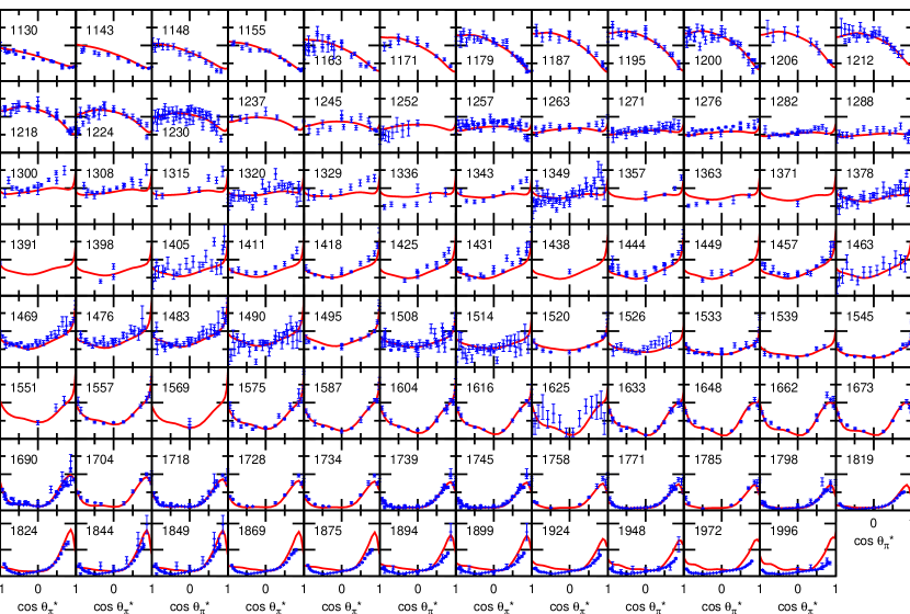
Figure 8: (Color online) Unpolarized differential cross sections, $d\sigma/d\Omega^{*}_{\pi}$ ($\mu$b/sr), for $\gamma n\to\pi^{-}p$. The data are from Refs. gn-pmp-1 ; gn-pmp-2 ; gn-pmp-3 ; gn-pmp-4 ; gn-pmp-5 ; gn-pmp-6 ; gn-pmp-7 ; gn-pmp-8 ; gn-pmp-9 ; gn-pmp-10 ; gn-pmp-11 ; gn-pmp-12 ; gn-pmp-13 ; gn-pmp-14 ; gn-pmp-15 ; gn-pmp-16 ; gn-pmp-17 ; gn-pmp-18 ; gn-pmp-19 ; gn-pmp-20 ; gn-pmp-21 ; gn-pmp-22 ; gn-pmp-23 ; gn-pmp-24 .

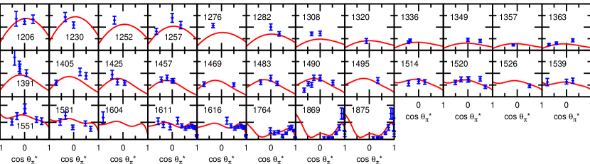
Figure 9: (Color online) Unpolarized differential cross sections $d\sigma/d\Omega^{*}_{\pi}$ ($\mu$b/sr), for $\gamma n\to\pi^{0}n$. The data are from Refs. gn-p0n-1 ; gn-p0n-2 ; gn-p0n-3 ; gn-p0n-4 .

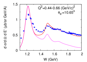
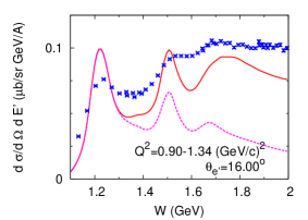
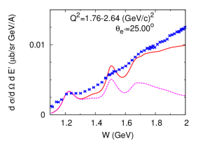
Figure 10: (Color online) Comparison of DCC-based calculation with data for differential cross sections per nucleon of inclusive electron-deuteron scattering at $E_{e}$=4.628 GeV. The red solid curves are for inclusive cross sections while the magenta dashed-curves are for contributions from the $\pi N$ final states. The range of $Q^{2}$ and the electron scattering angle ($\theta_{e^{\prime}}$) are indicated in each panel. The data are from Ref. en-incl .

We show unpolarized differential cross sections for $\gamma n\to\pi N$ calculated with the DCC model in comparison with data in Figs. 8 and 9, and find a reasonable agreement. We also show a comparison of the DCC-based calculation with data of differential cross sections per nucleon for the inclusive electron-deuteron scattering in Fig. 10. In this calculation, we simply take an average of electron-proton and electron-neutron differential cross sections in the free space. As seen in the figures, the calculated resonance peaks are sharper than the data, indicating that the smearing due to the Fermi motion and final state interaction needs to be taken into account to obtain a good agreement with the data hirata . Finally we note that a more comprehensive analysis including $\gamma n\to\pi N$ data is currently underway, which will be reported elsewhere neutron-dcc .

V Results for neutrino reactions

Before discussing neutrino reaction cross sections, first we examine the inclusive structure function $F^{\rm CC}_{2}$ defined in Eq. (17) at $Q^{2}$=0. At this particular kinematics, the neutrino cross sections are solely determined by $F^{\rm CC}_{2}$. $F^{\rm CC}_{2}(Q^{2}=0)$ has been often calculated with a PCAC model in which $F^{\rm CC}_{2}(Q^{2}=0)$ is related to (experimental) $\pi N$ total cross section by applying the PCAC hypothesis knls12 ; paschos-pcac . Within our DCC model, we can calculate $F^{\rm CC}_{2}(Q^{2}=0)$ either with the $\pi N$ amplitudes or with the hadronic axial-current amplitudes. In Fig. 11, we compare $F^{\rm CC}_{2}(Q^{2}=0)$ calculated by these two ways, and find a good agreement. Some comments are in order.

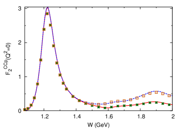
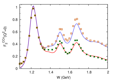
Figure 11: (Color online) The structure function $F^{\rm CC}_{2}$ at $Q^{2}=0$. $F^{\rm CC}_{2}$ calculated with the axial current amplitude (lines) are compared with those from $\pi N$ cross sections via the PCAC relation (points). The upper (lower) line and point are for inclusive ($\pi N$) final state(s). The left (right) panel is for CC $\nu$-proton/CC $\bar{\nu}$-neutron (CC $\nu$-neutron/CC $\bar{\nu}$-proton) process.

For the CC $\nu$-proton/CC $\bar{\nu}$-neutron process (left panel of Fig. 11), only $I$=3/2 resonances contribute, and the $\Delta(1232)$ dominates $F^{\rm CC}_{2}$ in low energies. On the other hand, for CC $\nu$-neutron/CC $\bar{\nu}$-proton process (right panel of Fig. 11), both $I$=1/2 and 3/2 resonances contribute. Thus not only the $\Delta(1232)$ but also $N(1535)~{}1/2^{-}$ and $N(1520)~{}3/2^{-}$ resonances in the second resonance region, $N(1675)~{}5/2^{-}$ and $N(1680)~{}5/2^{+}$ resonances in the third resonance region create characteristic energy dependence of $F^{\rm CC}_{2}$. Although we found the two calculations agree well by construction of the model, we still notice that the $\Delta(1232)$ peak from the axial-current amplitude somewhat overshoots that from the $\pi N$ model. Also, there are slight differences in the second and third resonance region in the right panel of Fig. 11. These differences originate from the fact that the spatial momentum transfer is fixed either at $Q^{2}$=0 or at $Q^{2}=-m^{2}_{\pi}$. For a more meaningful comparison, we could have compared the two $F^{\rm CC}_{2}$ calculated at the same $Q^{2}$. Indeed, we have confirmed a significantly better agreement between $F^{\rm CC}_{2}(Q^{2}=-m^{2}_{\pi})$ from the axial current amplitudes and those from the $\pi N$ cross sections, which should be the case by definition of the model. Here, we showed $F^{\rm CC}_{2}$ that is actually used in calculating the neutrino cross sections, and how much it can deviate from those obtained with the $\pi N$ cross sections. Also, we remark that even though most existing neutrino-nucleon reaction models in the resonance region have axial-currents based on the PCAC relation, they do not necessarily give $F^{\rm CC}_{2}(Q^{2}=0)$ in agreement with those from the $\pi N$ cross sections; we will come back to this point later in this section.

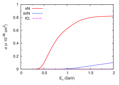
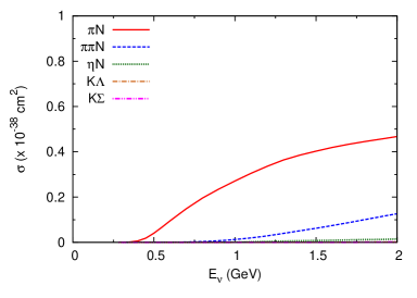
Figure 12: (Color online) Total cross sections for the CC $\nu_{\mu}\,p$ (left) and $\nu_{\mu}n$ (right) reactions.

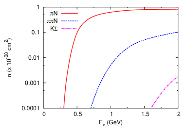
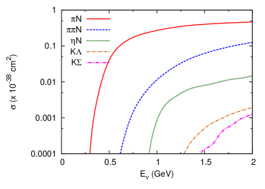
Figure 13: (Color online) The same as Fig. 12 but in log scale.

Now we present cross sections for the $\nu_{\mu}\,N$ reactions. With the DCC model, we can predict contributions from all the final states included in our model. Also, the DCC model provides all possible differential cross sections for each channel. Here, we present total cross sections for the CC $\nu_{\mu}\,N$ reactions up to $E_{\nu}=2$ GeV in Fig. 12; we also show them in Fig. 13 in log scale to see contributions from all of the final states. For the proton-target, the single pion production dominates in the considered energy region. For the neutron-target, the single pion production is still the largest, but double-pion production becomes relatively more important towards $E_{\nu}=2$ GeV. The $\eta N$ and $KY$ production cross sections are ${\cal O}(10^{-1}$-$10^{-2})$ smaller.

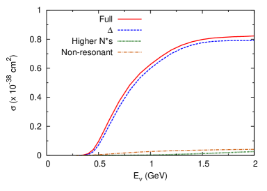
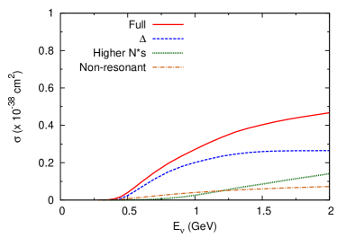
Figure 14: (Color online) Various mechanisms contributing to $\nu_{\mu}\,p\to\mu^{-}\pi^{+}p$ (left) and $\nu_{\mu}n\to\mu^{-}\pi N$ (right).

Next we examine reaction mechanisms of the $\nu_{\mu}\,N$ scattering. In Fig. 14, we break down the single-pion production cross sections into several contributions each of which contains a set of certain mechanisms. For the proton-target process, the contribution from the $\Delta$(1232) resonance dominates, while the higher $N^{*}$ contribution is very small. The $\Delta$ contribution here is the neutrino cross section calculated with the resonant amplitude, Eq. (34), of the $P_{33}$ partial wave only, while the higher $N^{*}$ contribution is from the resonant amplitude including all partial waves other than $P_{33}$. The non-resonant cross sections calculated from the non-resonant amplitude of Eq. (33) is small for the proton-target process. In contrast, the situation is more complex in the neutron-target process where the $\Delta$ gives a smaller contribution and both $I=$1/2 and 3/2 resonances contribute. As can be seen in the right panel of Fig. 14, the $\Delta$ dominates for $E_{\nu}\ \raise 1.29167pt\hbox{$<$\kern-7.5pt\lower 4.30554pt\hbox{$\sim$}}\ 1$ GeV, and higher resonances and non-resonant mechanisms give comparable contributions towards $E_{\nu}\sim 2$ GeV. This shows an importance of including both resonant and non-resonant contributions with the interferences among them under control, as has been stressed in Sec. III.4.2.

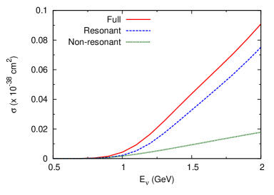
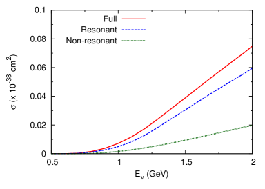
Figure 15: (Color online) Various mechanisms contributing to $\nu_{\mu}\,p\to\mu^{-}\pi^{+}\pi^{0}p$ (left) and $\nu_{\mu}n\to\mu^{-}\pi^{+}\pi^{-}p$ (right).

Similarly, the contribution of resonant and non-resonant amplitudes are shown in Fig. 15 for the two-pion production reaction. Because $\Delta(1232)$ mainly contributes below the $\pi\pi N$ production threshold and thus gives a small contribution here, the resonant and non-resonant contributions are more comparable. Still, the figures show that the resonance-excitations are the main mechanism for the double-pion production in this energy region.

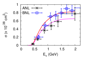
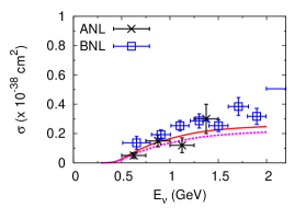
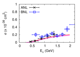
Figure 16: (Color online) Comparison of the DCC-based calculation (red solid curves) with data for $\nu_{\mu}\,p\to\mu^{-}\pi^{+}p$ (left), $\nu_{\mu}n\to\mu^{-}\pi^{0}p$ (middle) and $\nu_{\mu}n\to\mu^{-}\pi^{+}n$ (right). The DCC calculation with $0.8\times g_{AN\Delta(1232)}^{\rm PCAC}$ is also shown (magenta dashed curve). ANL (BNL) data are from Ref. anl (bnl ).

Next we compare the CC neutrino-induced single pion production cross sections from the DCC model with available data from Refs. anl ; bnl in Fig. 16. The left panel shows the total cross sections for $\nu_{\mu}\,p\to\mu^{-}\pi^{+}p$ for which $\Delta(1232)$ dominates as we have seen in Fig. 14. If the $\Delta(1232)$-dominance persists in the neutron-target processes shown in the middle and right panels of Fig. 16, the isospin Clebsch-Gordan coefficients determine the relative strength as $\sigma(\nu_{\mu}n\to\mu^{-}\pi^{0}p)/\sigma(\nu_{\mu}p\to\mu^{-}\pi^{+}p)=2/9\sim 0.22$, and $\sigma(\nu_{\mu}n\to\mu^{-}\pi^{+}n)/\sigma(\nu_{\mu}p\to\mu^{-}\pi^{+}p)=1/9\sim 0.11$. The actual ratios from the DCC model are $\sigma(\nu_{\mu}n\to\mu^{-}\pi^{0}p)/\sigma(\nu_{\mu}p\to\mu^{-}\pi^{+}p)=$ 0.28, 0.27, 0.29, and $\sigma(\nu_{\mu}n\to\mu^{-}\pi^{+}n)/\sigma(\nu_{\mu}p\to\mu^{-}\pi^{+}p)=$ 0.13, 0.17, 0.21 at $E_{\nu}$=0.5, 1, 1.5 GeV, respectively. The deviations from the naive isospin analysis are due to the the non-resonant and higher-resonances contributions mostly in the neutron-target processes, as we have seen in Fig. 14. The two datasets from BNL and ANL for $\nu_{\mu}p\to\mu^{-}\pi^{+}p$ shown in the left panel of Fig. 16 are not consistent as has been well known, and our result is closer to the BNL data anl . For the other channels, our result is fairly consistent with both of the BNL and ANL data. It seems that the bare axial $N$-$\Delta(1232)$ coupling constants determined by the PCAC relation are too large to reproduce the ANL data. Because axial $N$-$N^{*}$ coupling constants should be better determined by analyzing neutrino-reaction data, it is tempting to multiply the bare axial $N$-$\Delta(1232)$ coupling constants, $g_{AN\Delta(1232)}^{\rm PCAC}$, defined in Eq. (165) by 0.8, so that the DCC model better fits the ANL data. The resulting cross sections are shown by the dashed curves in Fig. 16. We find that $\sigma(\nu_{\mu}p\to\mu^{-}\pi^{+}p)$ is reduced due to the dominance of the $\Delta(1232)$ resonance in this channel, while $\sigma(\nu_{\mu}n\to\mu^{-}\pi N)$ is only slightly reduced. As mentioned in the introduction, the original data of these two experimental data have been reanalyzed recently reanalysis , and it is pointed out that the discrepancy between the two datasets is resolved. The resulting cross sections are closer to the previous ANL data. However, the number of data is still very limited, and a new measurement of neutrino cross sections on the hydrogen and deuterium is highly desirable. We also note that the data shown in Fig. 16 were taken from experiments using the deuterium target. Thus one should analyze the data considering the nuclear effects such as the initial two-nucleon correlation and the final state interactions. Recently, the authors of Ref. wsl have taken a first step towards such an analysis. They developed a model that consists of elementary amplitudes for neutrino-induced single pion production off the nucleon sul , pion-nucleon rescattering amplitudes, and the deuteron and final $NN$ scattering wave functions. Although they did not analyze the ANL and BNL data with their model, they examined how much the cross sections at certain kinematics can be changed by considering the nuclear effects. They found that the cross sections can be reduced as much as 30% for $\nu_{\mu}d\to\mu^{-}\pi^{+}pn$ due to the $NN$ rescattering. Meanwhile, the cross sections for $\nu_{\mu}d\to\mu^{-}\pi^{0}pp$ are hardly changed by the final state interaction. It will be important to analyze the ANL and BNL data with this kind of model to determine the axial nucleon current, particularly the axial $N$-$\Delta$(1232) transition strength.

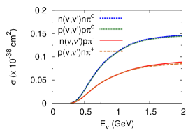
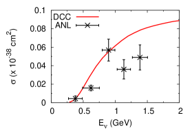
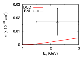
Figure 17: (Color online) (left) DCC-based calculation for NC neutrino-induced single pion productions. (middle) Comparison of the DCC model and ANL data NC-data for $\nu n\to\nu p\pi^{-}$. (right) Comparison of the DCC model and BNL data KL-data for $\nu n\to\mu^{-}K^{+}\Lambda$.

Regarding the NC single pion production, we show results in Fig. 17. In the left panel, we show the cross sections for all final charge states. The ratios $\sigma(\nu p\to\nu p\pi^{0})/\sigma(\nu p\to\nu n\pi^{+})\sim\sigma(\nu n\to\nu n\pi^{0})/\sigma(\nu n\to\nu p\pi^{-})\sim 2$ can be mostly understood from the isospin Clebsch-Gordan coefficient accompanied by the $\Delta\to\pi N$ vertex. A slight difference between $\sigma(\nu p\to\nu p\pi^{0})$ and $\sigma(\nu n\to\nu n\pi^{0})$ [also between $\sigma(\nu p\to\nu n\pi^{+})$ and $\sigma(\nu n\to\nu p\pi^{-})$] is mostly from different interference patterns between the isovector and isoscalar currents. In the middle panel of Fig. 17, we compare the NC $\nu n\to\nu p\pi^{-}$ cross sections from the DCC model with ANL data NC-data , and find a fair consistency. In closing this paragraph, we compare our DCC-based result for another single meson production, $\nu n\to\mu^{-}K^{+}\Lambda$, with data in the right panel of Fig. 17. Although our result undershoots the data, the data are based on statistically very limited number of events (3 events) and we still cannot say something conclusive.

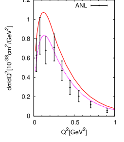
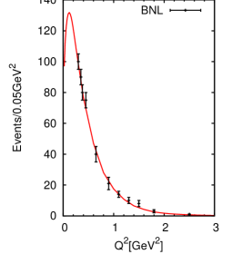
Figure 18: (Color online) The flux-averaged (0.5 GeV $\leq E_{\nu}\leq$ 6 GeV) $d\sigma/dQ^{2}$ for $\nu_{\mu}\,p\to\mu^{-}\pi^{+}p$. (Left) The DCC-based calculation (red solid curve) is compared with the ANL data anl . The DCC calculation with $0.8\times g_{AN\Delta(1232)}^{\rm PCAC}$ is also shown (magenta dashed curve). Contributions from high $W$ ($>$1.4 GeV) are cut in the calculation in order to be consistent with the data. (Right) The DCC-based calculation (red solid curve) is compared with the BNL data bnl .

We also compare our calculation of the single pion production with data for differential cross sections with respect to $Q^{2}$ ($d\sigma/dQ^{2}$). To make contact with the data in Refs. anl ; data90 , we calculate the following flux-averaged cross sections:

$$\frac{d\bar{\sigma}}{dQ^{2}}={\displaystyle\int_{E_{\rm min}}^{E_{\rm max}}dE_{\nu}\frac{N(E_{\nu})}{\sigma_{\rm model}(E_{\nu})}\frac{d\sigma_{\rm model}}{dQ^{2}}(E_{\nu})\over\displaystyle\int_{E_{min}}^{E_{max}}dE_{\nu}\frac{N(E_{\nu})}{\sigma_{\rm model}(E_{\nu})}}\ ,$$ (44)

where $N(E_{\nu})$ is the number of events at neutrino energy $E_{\nu}$, and is given in Fig. 6 of Ref. anl and Fig. 4 of Ref. data90 . The DCC model gives cross sections denoted as $\sigma_{\rm model}(E_{\nu})$. In the left panel of Fig. 18, we compare the DCC-based calculation with the ANL data anl . We find here again that the DCC model overshoots the ANL data for $\nu_{\mu}\,p\to\mu^{-}\pi^{+}p$. This tempts us to plot $d\sigma/dQ^{2}$ obtained with the bare axial $N$-$\Delta(1232)$ coupling constants, $g_{AN\Delta(1232)}({\rm PCAC})$, multiplied by 0.8, as we did in Fig. 16(left). This result is in better agreement with the ANL data as seen in Fig. 18 (left). The assumed dipole form factor ($M_{A}=1.02$ GeV) for the bare axial $N$-$\Delta(1232)$ vertex seems fairly consistent with the data. In the right panel of Fig. 18, we compare the DCC-based calculation with the BNL data data90 . The $Q^{2}$-dependence of the BNL data with the arbitrary scale is well explained with our DCC model.

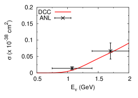
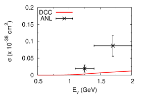
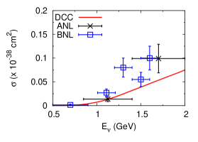
Figure 19: (Color online) Comparison of the DCC-based calculation with data for $\nu_{\mu}\,p\to\mu^{-}\pi^{+}\pi^{0}p$ (left), $\nu_{\mu}p\to\mu^{-}\pi^{+}\pi^{+}n$ (middle) and $\nu_{\mu}n\to\mu^{-}\pi^{+}\pi^{-}p$ (right). ANL (BNL) data are from Ref. anl2 (bnl ).

We finally compare our results for double-pion productions with existing data in Fig. 19. Although there exist a few theoretical works on the neutrino-induced double-pion production near threshold biswas ; adjei ; spain-pipin , our calculation for the first time takes account of relevant resonance contributions for this process. The DCC-based prediction is fairly consistent with the data in the order of the magnitude. Particularly, the cross sections for $\nu_{\mu}\,p\to\mu^{-}\pi^{+}\pi^{0}p$ from the DCC model are in agreement with data. However, the DCC prediction underestimates the $\nu_{\mu}\,p\to\mu^{-}\pi^{+}\pi^{+}n$ data. The rather small ratio of $\sigma(\nu_{\mu}\,p\to\mu^{-}\pi^{+}\pi^{+}n)/\sigma(\nu_{\mu}\,p\to\mu^{-}\pi^{+}\pi^{0}p)\sim 13\%$ at $E_{\nu}$=2 GeV from our calculation can be understood as follows. Within the present DCC-based calculation, $\pi\pi N$ final states are from decays of the $\pi N$ and of the $\pi\Delta$, $\rho N$, $\sigma N$ quasi two-body states. For a neutrino CC process on the proton for which hadronic states have $I=3/2$, the $\pi N$, $\pi\Delta$, $\rho N$ channels can contribute. Within the current DCC model, we found that the $\pi\Delta$ channel gives a dominant contribution to the double pion productions. Then, retaining only the $\pi\Delta$ contribution, the ratio is given by the isospin Clebsch-Gordan coefficients as, $\sigma(\nu_{\mu}\,p\to\mu^{-}\pi^{+}\pi^{+}n)/\sigma(\nu_{\mu}\,p\to\mu^{-}\pi^{+}\pi^{0}p)=2/13\sim 15\%$, in good agreement with the ratio from the full calculation. With a very limited dataset, we do not further pursue the origin of the difference between our calculation and the data. If the double-pion data are further confirmed, then the model needs to incorporate some other mechanisms and/or adjust model parameters of the DCC model to explain the data.

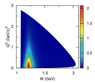
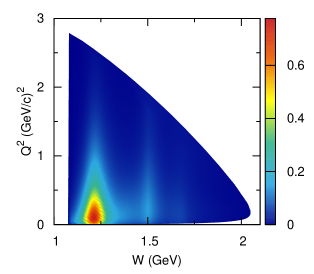
Figure 20: (Color online) Contour plots of $d^{2}\sigma/dWdQ^{2}$ for $\nu_{\mu}\,p\to\mu^{-}\pi^{+}p$ (left) and $\nu_{\mu}n\to\mu^{-}\pi N$ (right) at $E_{\nu}=2$ GeV.

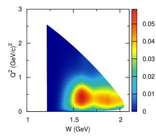
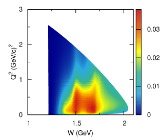
Figure 21: (Color online) Contour plots of $d^{2}\sigma/dWdQ^{2}$ for $\nu_{\mu}\,p\to\mu^{-}\pi^{+}\pi^{0}p$ (left) and $\nu_{\mu}n\to\mu^{-}\pi^{+}\pi^{-}p$ (right) at $E_{\nu}=2$ GeV.

Important and characteristic hadronic dynamics changes as $W$ and $Q^{2}$ change. Thus, it would be interesting to see double-differential cross sections, $d^{2}\sigma/dWdQ^{2}$, as shown in Fig. 20 for the single-pion productions. The prominent peak due to $\Delta(1232)$ has a long tail toward higher $Q^{2}$ region. For the neutron-target, the resonant behavior in the second resonance region is also seen. Similar contour plots are also shown for double-pion productions in Fig. 21. Here, the situation is very different from the single pion case, and the main contributors are resonances in the second and third resonance regions.

Since a comparison of the DCC model with other models is interesting, we compare in Figs. 22 and 23 the structure function $F^{\rm CC}_{2}(Q^{2}=0)$ of the DCC model with the model due to Lalakulich et al. lalakulich (LPP model), and the Rein-Sehgal (RS) model RS ; RS2 .

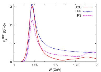
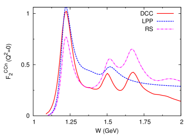
Figure 22: (Color online) $F^{\rm CC}_{2}$ at $Q^{2}=0$ from contribution of the single pion production only. The DCC model is compared with the LPP model due to Lalakulich et al. lalakulich and the Rein-Sehgal (RS) model RS ; RS2 . The left (right) panel is for the CC $\nu_{\mu}\,p$ ($\nu_{\mu}\,n$) reaction.

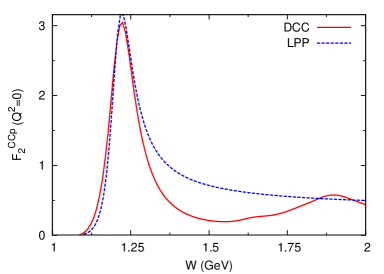
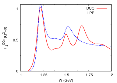
Figure 23: (Color online) The inclusive structure function $F^{\rm CC}_{2}$ at $Q^{2}=0$. The other features are the same as those in Fig. 22.

The LPP model consists of four amplitudes of the Breit-Wigner form for $\Delta(1232)~{}3/2^{+}$, $N(1535)~{}1/2^{-}$, $N(1440)~{}1/2^{+}$ and $N(1520)~{}3/2^{-}$ resonances with no background. The RS model consists of 18 Breit-Wigner terms plus a non-interfering non-resonant background of $I=1/2$. On the left (right) panel of Fig. 22, we show $F^{\rm CC}_{2}$ for the CC reaction on the proton (neutron) going to the $\pi N$ final state. From the comparison, a good agreement between the DCC model and the LPP model is found only near the $\Delta(1232)$ peak; otherwise they are rather different. The RS model rather undershoot the $\Delta(1232)$ peak, as has been also pointed out in Refs. AHN ; RS-ff ; leitner ; nuint12 . Near the threshold ($W\sim$ 1.1 GeV), meanwhile, $F^{\rm CC}_{2}(Q^{2}=0)$ of the DCC model is larger than those of the LPP and RS models. A similar tendency persists in the inclusive $F^{\rm CC}_{2}$ as shown in Fig. 23. For the LPP model, $F_{2}^{{\rm CC}p}$ in the left panels of Figs. 22 and 23 are the same because only the $\Delta(1232)$ contributes to the proton-target process, and it decays almost exclusively into the $\pi N$ state. As discussed earlier in this paper, $F^{\rm CC}_{2}$ at $Q^{2}=0$ is related to the $\pi N$ cross sections through the PCAC relation, and thus is given almost model-independently. We have shown in Fig. 11 that $F^{\rm CC}_{2}$ from the DCC axial current model and that from the precise $\pi N$ model agree well in accordance with the PCAC relation. Therefore, the difference between the DCC model and the LPP and the RS models in $F^{\rm CC}_{2}(Q^{2}=0)$ reveals a consequence of missing the consistency between the axial-current and the $\pi N$ interaction in the latter models.

VI Conclusion

In this work, we have developed a dynamical coupled-channels (DCC) model for neutrino-nucleon reactions in the resonance region. Our starting point is the DCC model that we have developed through a comprehensive analysis of $\pi N,\gamma p\to\pi N,\eta N,K\Lambda,K\Sigma$ data for $W\leq 2.1$ GeV knls13 . The model has also been shown to give a reasonable description of $\pi N\to\pi\pi N$ kamano-pipin . In order to extend the DCC model of Ref. knls13 to what works for the neutrino reactions, we analyzed data for the single pion photoproduction off the neutron, and also data for the electron scattering on both proton and neutron targets. Through the analysis, we determined the $Q^{2}$-dependence of the vector form factors up to $Q^{2}\leq 3$ (GeV/$c$)². By combining the vector form factors for the proton and neutron, we separated the vector form factors into the isovector and isoscalar parts; this isospin separation is a necessary step to apply the model to the neutrino reactions. We also derived the axial-current matrix elements. An appealing point of our approach is that we can derive the axial-current matrix elements that are linked to the $\pi N$ potential of the DCC model through the PCAC relation. As a consequence, relative phases between the non-resonant and resonant axial current amplitudes are uniquely determined within the DCC model. The $Q^{2}$-dependences of the axial form factors are difficult to determine with the available data. Thus we used the same axial form factors for all the axial $N$-$N^{*}$ vertices. Although this prescription is what we can do best for the moment, we hope to improve this in future if more data become available. Then, the preparation for calculating the neutrino-induced meson productions off the nucleon is completed.

We have presented cross sections for the neutrino-induced meson productions for $E_{\nu}\leq 2$ GeV. In this energy region, the single-pion production gives the largest contribution. Towards $E_{\nu}\sim 2$ GeV, the cross section for the double-pion production is getting larger to become 1/8 (1/4) of the single-pion production cross section for the proton (neutron) target. Because our DCC model has been determined by analyzing the $\pi N,\gamma N\to\pi N,\eta N,K\Lambda,K\Sigma$ data, we can also make a quantitative prediction for the neutrino cross sections for $\eta N$, $K\Lambda$, and $K\Sigma$ productions. We found that cross sections for $\eta N,K\Lambda$ and $K\Sigma$ productions are $10^{-2}$-$10^{-3}$ times smaller than those for the single pion production. We have compared our numerical results with the available experimental data. For the single-pion production, our result, for which the axial $N$-$N^{*}$ couplings are fixed by the PCAC relation, is consistent with the BNL data for $\nu_{\mu}p\to\mu^{-}\pi^{+}p$, while fair agreement with both ANL and BNL data is found for the neutron target data. Through the comparison with the single pion production data for $W\ \raise 1.29167pt\hbox{$<$\kern-7.5pt\lower 4.30554pt\hbox{$\sim$}}\$1.4 GeV for which the $\Delta(1232)$-excitation is the dominant mechanism, we were able to study the strength and the $Q^{2}$-dependence of the axial $N$-$\Delta(1232)$ coupling. We also calculated double-pion production cross sections by taking account of relevant resonance contributions for the first time, and compared them with the data. We found a good agreement for $\nu_{\mu}\,p\to\mu^{-}\pi^{+}\pi^{0}p$ and $\nu_{\mu}n\to\mu^{-}\pi^{+}\pi^{-}p$, but not for $\nu_{\mu}p\to\mu^{-}\pi^{+}\pi^{+}n$. Because the data are statistically rather poor, it is difficult to make a conclusive judgement on the DCC model. We hope new high quality data will become available in near future. We examined reaction mechanisms contributing to the single-pion production. For the proton target where only $I=3/2$ states contribute, the $\Delta(1232)$ dominates. However, for the neutron target where both $I=1/2$ and 3/2 states contribute, the $\Delta(1232)$, higher $N^{*}$ resonances, and non-resonant mechanisms give comparable contributions towards $E_{\nu}\sim 2$ GeV. Thus it is very important to have interference patterns among those different mechanisms under control. In this regard, our DCC approach has an advantage over the other existing models, as mentioned in the above paragraph.

Finally, we make some remarks on our future prospect. Our DCC model should be smoothly connected to a DIS model in the resonance-DIS overlapping region. Because the DCC model still has degrees of freedom to vary the $Q^{2}$-dependence of the axial form factors, we can adjust them to fit the $W$- and $Q^{2}$-dependences of inclusive cross sections from the DIS model in the overlapping region. This needs be done in a future work. Having developed the DCC neutrino-nucleon reaction model that covers the whole resonance region, next task should be developing a neutrino-nucleus reaction model in which the DCC model describes the elementary processes. The simplest case is the neutrino-deuteron reactions, and for that, we can do a relatively well-established quantum mechanical calculation, as done in Ref. wsl . It will be interesting to extend the work of Ref. wsl by replacing the elementary amplitudes therein with those from the DCC model developed here. Then, ANL and BNL data should be reanalyzed with this model that takes care of not only the Fermi motion but also the final state interactions (FSI). The importance of FSI has been demonstrated in Ref. wsl . Also, this development can serve as a preparation for a possible T2K experiment wilking that utilizes heavy-water (D₂O) as the target. Application to heavier nuclei will also be very important. In the $\Delta(1232)$ region, the well-developed $\Delta$-hole model D-hole1 ; D-hole2 may give a hint to address pion productions in the neutrino-nucleus reaction. For even higher energy neutrino reactions, a fully quantum mechanical calculation seems formidable. Combining the elementary amplitudes of the DCC model with a hadron transport model may be a possible and practical option, as has been done in the literature gibuu ; spain-cascade .

Appendix A Matrix elements of non-resonant axial currents

We explained in Sec. III.3 how to derive matrix elements of non-resonant axial-currents to be implemented in the DCC model. Here, we present tree-level, non pion-pole (NP) part of the matrix elements for a single meson production, $\langle M(k^{\prime},j)B(p^{\prime})|A^{i}_{\mu}(q)|N(p)\rangle$, where $i$ and $j$ are isospin components and the other variables in the parentheses are four-momenta carried by the corresponding nucleon ($N$), baryon ($B$), meson ($M$), and axial-current ($A_{\mu}$); labels for the spin and isospin states for the baryons are suppressed. The following expressions in Appendices A-C are those in the center-of-mass frame of the hadronic system (hCM). The matrix elements can be expressed in the following form:

$$\langle{M(k^{\prime}j),B(p^{\prime})}|A^{i}_{{\rm NP,tree}}(q)\cdot\epsilon(\lambda)|{N(p)}\rangle$$ (45)

$$= \frac{1}{(2\pi)^{3}}\sum_{n}\sqrt{\frac{m_{N}m_{B}}{E_{N}(-\bm{q})E_{B}(-\bm{k}^{\prime})2E_{M}(\bm{k}^{\prime})}}\bar{u}_{B}(-\bm{k}^{\prime})\bar{A}(n)u_{N}(-\bm{q})\,,$$

where $\epsilon^{\mu}(\lambda)$ is the polarization vector for the hadron axial current with a polarization $\lambda$. The Dirac spinor for the baryon $B$ is denoted by $u_{B}(\bm{p})$ that is also supposed to implicitly contain the isospin spinor. In the following subsections, we present expressions for $\bar{A}(n)$ for each process labeled by the index $n$. $\bar{A}(n)$ is composed of several terms, denoted as $\bar{A}^{n}_{a}$, $\bar{A}^{n}_{b}$,…, etc. for which we also present diagrammatic representations in TABLE 1. It is noted that, in evaluating the time component of four-momenta contained in the propagators in the following equations, we follow the definite procedures defined by the unitary transformation method sko ; sl ; see also Appendix C of Ref. msl07 .

For the axial-current matrix elements shown in the following subsections, we include at each vertex a dipole form factor in the same way as those used for $\pi N\to MB$ potentials in Ref. knls13 . For a meson-baryon-baryon vertex, we include a form factor of the form

$$F(\bm{k},\Lambda)=\left(\Lambda^{2}\over\bm{k}^{2}+\Lambda^{2}\right)^{2}$$ (46)

where $\bm{k}$ and $\Lambda$ are the meson momentum and the cutoff, respectively. For a $N$-$B$ transition vertex induced by the axial current, we also include a form factor of Eq. (46) in which $\bm{k}$ is chosen to satisfy

$$W=\sqrt{\bm{k}^{2}+m^{2}_{\pi}}+\sqrt{\bm{k}^{2}+m^{2}_{N}}\ ,$$ (47)

in order to satisfy the PCAC relation, Eq. (37). In a $t$-channel diagram, there is a meson-meson transition vertex induced by the axial-current, and we use a dipole form factor of Eq. (46) where $\bm{k}$ being the momentum of the exchanged meson. For a contact term, we use double dipole form factor, $F(\bm{k}^{\prime},\Lambda)F(\bm{k},\Lambda)$, where $\bm{k}^{\prime}$ is the outgoing meson momentum. In addition to this hadronic form factor, we also include the axial form factor of the dipole form, as discussed in Sec. III.3, to take care of the $Q^{2}$-dependence of the axial couplings.

In the following expressions, we use notations such as $\tilde{k}=p-p^{\prime}$ and $k$ that satisfies Eq. (47). We also denote $\epsilon^{\mu}$ for $\epsilon^{\mu}(\lambda)$ for simplicity. The $i$-th component of Pauli matrix that acts on the nucleon isospin spinors is denoted by $\tau^{i}$. We denote the pseudoscalar, vector, and scalar mesons by $P$, $V$, and $S$, respectively, and the octet and decuplet baryons by $B$. With this notation, the $PBB^{\prime}$, $VBB^{\prime}$, and $SBB^{\prime}$ coupling constants are denoted respectively by $f_{PBB^{\prime}}$, $g_{VBB^{\prime}}$, and $g_{SBB^{\prime}}$, while the $PP^{\prime}V$ and $PP^{\prime}S$ coupling constants are denoted by $g_{PP^{\prime}V}$ and $g_{PP^{\prime}S}$, respectively. The tensor coupling constant of a $VBB^{\prime}$ coupling is denoted by $\kappa_{V}$. For numerical values of couplings, masses, cutoffs appearing below in this appendix, we use those determined in Ref. knls13 , and listed in TABLEs XI-XIII of the reference. In addition, we use $f_{\pi}=93$ MeV.

Table 1: Diagrammatic representations for non-resonant axial-current matrix elements. $\bar{A}^{n}_{a}$, $\bar{A}^{n}_{b}$,… correspond to expressions presented in Eqs. (53)-(137). The wavy lines represent the external axial-currents.

$MB=\pi N$	$\bar{A}^{1}_{a}$	$\bar{A}^{1}_{b}$	$\bar{A}^{1}_{c}$	$\bar{A}^{1}_{d}$,$\bar{A}^{1}_{e}$,$\bar{A}^{1}_{f}$	$\bar{A}^{1}_{g}$	$\bar{A}^{1}_{h}$
$\eta N$	$\bar{A}^{2}_{a}$	$\bar{A}^{2}_{b}$
$\sigma N$	$\bar{A}^{3}_{a}$	$\bar{A}^{3}_{b}$		$\bar{A}^{3}_{c}$
$\rho N$	$\bar{A}^{4}_{a}$	$\bar{A}^{4}_{b}$		$\bar{A}^{4}_{c}$,$\bar{A}^{4}_{e}$		$\bar{A}^{4}_{d}$
$\pi\Delta$	$\bar{A}^{5}_{a}$	$\bar{A}^{5}_{b}$	$\bar{A}^{5}_{d}$	$\bar{A}^{5}_{c}$
$K\Lambda$	$\bar{A}^{6}_{a}$	$\bar{A}^{6}_{b}$	$\bar{A}^{6}_{c}$	$\bar{A}^{6}_{d}$,$\bar{A}^{6}_{e}$
$K\Sigma$	$\bar{A}^{7}_{a}$	$\bar{A}^{7}_{b}$,$\bar{A}^{7}_{c}$	$\bar{A}^{7}_{d}$	$\bar{A}^{7}_{e}$,$\bar{A}^{7}_{f}$

A.1 $MB=\pi N$

$$\bar{A}(1)=\bar{A}^{1}_{a}+\bar{A}^{1}_{b}+\bar{A}^{1}_{c}+\bar{A}^{1}_{d}+\bar{A}^{1}_{e}+\bar{A}^{1}_{f}+\bar{A}^{1}_{g}+\bar{A}^{1}_{h}\ ,$$ (48)

with

$$\bar{A}^{1}_{a} = if_{\pi}\left(\frac{f_{\pi NN}}{m_{\pi}}\right)^{2}\not\!{k}^{\prime}\gamma_{5}\tau^{j}{1\over\ooalign{\hfil/\hfil\crcr$p$}^{\prime}+\ooalign{\hfil/\hfil\crcr$k$}^{\prime}-m_{N}}\not\!{\epsilon}\gamma_{5}\tau^{i}\ ,$$ (53)

$$\bar{A}^{1}_{b} = if_{\pi}\left(\frac{f_{\pi NN}}{m_{\pi}}\right)^{2}\not\!{\epsilon}\gamma_{5}\tau^{i}{1\over\ooalign{\hfil/\hfil\crcr$p$}-\ooalign{\hfil/\hfil\crcr$k$}^{\prime}-m_{N}}\not\!{k}^{\prime}\gamma_{5}\tau^{j}\ ,$$ (58)

$$\bar{A}^{1}_{c} = if_{\pi}\left(\frac{f_{\pi N\Delta}}{m_{\pi}}\right)^{2}{\epsilon}_{\alpha}(T^{\dagger})^{i}S^{\alpha\beta}_{\Delta}(p-k^{\prime}){k}^{\prime}_{\beta}T^{j}\ ,$$ (59)

$$\bar{A}^{1}_{d} = -iC_{V1}\frac{f_{\pi}g_{\rho NN}g_{\rho\pi\pi}}{m_{\rho}^{2}}\left[\not\!{\epsilon}+C_{V2}\frac{\kappa_{\rho}}{4m_{N}}(\not\!{\epsilon}\not\!{\tilde{k}}-\not\!{\tilde{k}}\not\!{\epsilon})\right]i\epsilon_{jil}\tau^{l}$$ (60)

$$+if_{\pi}g_{\rho NN}g_{\rho\pi\pi}\frac{\tilde{k}^{2}}{m^{2}_{\rho}(\tilde{k}^{2}-m^{2}_{\rho})}\left[\not\!{\epsilon}+\frac{\kappa_{\rho}}{4m_{N}}(\not\!{\epsilon}\not\!{\tilde{k}}-\not\!{\tilde{k}}\not\!{\epsilon})\right]i\epsilon_{jil}\tau^{l}\ ,$$

$$\bar{A}^{1}_{e} = +if_{\pi}C_{S}{\epsilon^{3}\over|\bm{q}|}\frac{k\cdot k^{\prime}}{m_{\pi}}\delta_{ij}$$ (61)

$$-i\left(f_{\pi}g_{\sigma NN}g_{\sigma\pi\pi}\frac{\tilde{k}^{2}}{m_{\sigma}^{2}(\tilde{k}^{2}-m_{\sigma}^{2})}+f_{\pi}g_{f_{0}NN}g_{f_{0}\pi\pi}\frac{\tilde{k}^{2}}{m_{f_{0}}^{2}(\tilde{k}^{2}-m_{f_{0}}^{2})}\right){\epsilon^{3}\over|\bm{q}|}\frac{k\cdot k^{\prime}}{m_{\pi}}\delta_{ij}\ ,$$

$$\bar{A}^{1}_{f} = -if_{\pi}{\epsilon^{3}\over|\bm{q}|}\frac{g_{\sigma NN}\tilde{g}_{\sigma\pi\pi}m_{\pi}^{2}}{f_{\pi}}\frac{1}{\tilde{k}^{2}-m_{\sigma}^{2}}\delta_{ij}\ ,$$ (62)

$$\bar{A}^{1}_{g} = if_{\pi}\left(\frac{f_{\pi N\Delta}}{m_{\pi}}\right)^{2}{k}^{\prime}_{\alpha}(T^{\dagger})^{j}\left[S^{\alpha\beta}_{\Delta}(p^{\prime}+k^{\prime})-S^{(+)\alpha\beta}_{\Delta}(p^{\prime}+k^{\prime})\right]{\epsilon}_{\beta}T^{i}\ ,$$ (63)

where $S^{(+)\alpha\beta}_{\Delta}$ is the positive energy part of the $\Delta$ propagator; in the frame where the $\Delta$ is at rest,

$$S^{(+)mn}_{\Delta}(p)={1\over 6}{1+\gamma^{0}\over p^{0}-m_{\Delta}}(3\delta_{mn}-\sigma_{m}\sigma_{n})\ .$$ (64)

Also, the operator $T$ ($T^{\dagger}$) generates an isospin transition from $I=1/2$ to 3/2 ($I=3/2$ to 1/2) states. We note here that we include the cross diagram of $s$-channel $\Delta(1232)$-resonance diagram as a part of the non-resonant mechanism, as in Eq. (59). For $S_{31}$ partial wave, we also add

$$\bar{A}^{1}_{h} = if_{\pi}{\epsilon^{3}\over|\bm{q}|}c_{S_{31}}\ .$$ (65)

A.2 $MB=\eta N$

$$\bar{A}(2)=\bar{A}^{2}_{a}+\bar{A}^{2}_{b}\ ,$$ (66)

with

$$\bar{A}^{2}_{a} = if_{\pi}\frac{f_{\pi NN}f_{\eta NN}}{m_{\pi}m_{\eta}}\not\!{k}^{\prime}\gamma_{5}{1\over\ooalign{\hfil/\hfil\crcr$p$}^{\prime}+\ooalign{\hfil/\hfil\crcr$k$}^{\prime}-m_{N}}\not\!{\epsilon}\gamma_{5}\tau^{i}\ ,$$ (71)

$$\bar{A}^{2}_{b} = if_{\pi}\frac{f_{\pi NN}f_{\eta NN}}{m_{\pi}m_{\eta}}\not\!{\epsilon}\gamma_{5}\tau^{i}{1\over\ooalign{\hfil/\hfil\crcr$p$}-\ooalign{\hfil/\hfil\crcr$k$}^{\prime}-m_{N}}\not\!{k}^{\prime}\gamma_{5}\ .$$ (76)

A.3 $MB=\sigma N$

$$\bar{A}(3)=\bar{A}^{3}_{a}+\bar{A}^{3}_{b}+\bar{A}^{3}_{c}\ ,$$ (77)

with

$$\bar{A}^{3}_{a} = -f_{\pi}\frac{f_{\pi NN}}{m_{\pi}}g_{\sigma NN}{1\over\ooalign{\hfil/\hfil\crcr$p$}^{\prime}+\ooalign{\hfil/\hfil\crcr$k$}^{\prime}-m_{N}}\not\!{\epsilon}\gamma_{5}\tau^{i}\ ,$$ (82)

$$\bar{A}^{3}_{b} = -f_{\pi}\frac{f_{\pi NN}}{m_{\pi}}g_{\sigma NN}\not\!{\epsilon}\gamma_{5}{1\over\ooalign{\hfil/\hfil\crcr$p$}-\ooalign{\hfil/\hfil\crcr$k$}^{\prime}-m_{N}}\tau^{i}\ ,$$ (87)

$$\bar{A}^{3}_{c} = -f_{\pi}\frac{f_{\pi NN}g_{\sigma\pi\pi}}{m_{\pi}^{2}}\not\!{\tilde{k}}\gamma_{5}\tau^{i}\frac{\tilde{k}\cdot\epsilon}{\tilde{k}^{2}-m^{2}_{\pi}}\ .$$ (88)

A.4 $MB=\rho^{\prime}N$

$$\bar{A}(4)=\bar{A}^{4}_{a}+\bar{A}^{4}_{b}+\bar{A}^{4}_{c}+\bar{A}^{4}_{d}+\bar{A}^{4}_{e}\ ,$$ (89)

with

$$\bar{A}^{4}_{a} = -f_{\pi}\frac{f_{\pi NN}}{m_{\pi}}g_{\rho NN}\Gamma_{\rho^{\prime}}{1\over\ooalign{\hfil/\hfil\crcr$p$}^{\prime}+\ooalign{\hfil/\hfil\crcr$k$}^{\prime}-m_{N}}\not\!{\epsilon}\gamma_{5}\tau^{i}\ ,$$ (94)

$$\bar{A}^{4}_{b} = -f_{\pi}\frac{f_{\pi NN}}{m_{\pi}}g_{\rho NN}\not\!{\epsilon}\gamma_{5}\tau^{i}{1\over\ooalign{\hfil/\hfil\crcr$p$}-\ooalign{\hfil/\hfil\crcr$k$}^{\prime}-m_{N}}\Gamma_{\rho^{\prime}}\ ,$$ (99)

$$\bar{A}^{4}_{c} = -2if_{\pi}\frac{f_{\pi NN}}{m_{\pi}}g_{\rho\pi\pi}\epsilon_{ijl}\tau^{l}\frac{\epsilon\cdot\epsilon_{\rho^{\prime}}^{*}\not\!{\tilde{k}}\gamma_{5}}{\tilde{k}^{2}-m_{\pi}^{2}}\ ,$$ (100)

$$\bar{A}^{4}_{d} = -if_{\pi}{\epsilon^{3}\over|\bm{q}|}\frac{f_{\pi NN}}{m_{\pi}}g_{\rho NN}\not\!{\epsilon_{\rho^{\prime}}}^{*}\gamma_{5}\epsilon_{jil}\tau^{l}\ ,$$ (101)

$$\bar{A}^{4}_{e} = if_{\pi}\frac{g_{\omega NN}g_{\omega\pi\rho}}{m_{\omega}}\delta_{ij}\frac{\epsilon^{\alpha\beta\gamma\delta}\epsilon_{\rho^{\prime}\alpha}^{*}k^{\prime}_{\beta}\epsilon_{\gamma}}{\tilde{k}^{2}-m^{2}_{\omega}}\left[\gamma_{\delta}+\frac{\kappa_{\omega}}{4m_{N}}(\gamma_{\delta}\not\!{\tilde{k}}-\not\!{\tilde{k}}\gamma_{\delta})\right]\ ,$$ (102)

where $\epsilon_{\rho^{\prime}}^{*\mu}$ is the polarization vector for the $\rho$-meson, and

$$\Gamma_{\rho^{\prime}} = \frac{\tau^{j}}{2}\left[\not\!{\epsilon_{\rho^{\prime}}}^{*}+\frac{\kappa_{\rho}}{4m_{N}}(\not\!{\epsilon_{\rho^{\prime}}}^{*}\not\!{k}^{\prime}-\not\!{k}^{\prime}\not\!{\epsilon_{\rho^{\prime}}}^{*})\right]\ ,$$ (103)

and $\epsilon^{0123}=+1$ convention is taken.

A.5 $MB=\pi\Delta$

$$\bar{A}(5)=\bar{A}^{5}_{a}+\bar{A}^{5}_{b}+\bar{A}^{5}_{c}+\bar{A}^{5}_{d}\ ,$$ (104)

with

$$\bar{A}^{5}_{a} = if_{\pi}\frac{f_{\pi NN}f_{\pi N\Delta}}{m_{\pi}^{2}}T^{j}\epsilon_{\Delta}^{*}\cdot k^{\prime}{1\over\ooalign{\hfil/\hfil\crcr$p$}^{\prime}+\ooalign{\hfil/\hfil\crcr$k$}^{\prime}-m_{N}}\not\!{\epsilon}\gamma_{5}\tau^{i}\ ,$$ (109)

$$\bar{A}^{5}_{b} = if_{\pi}\frac{f_{\pi NN}f_{\pi N\Delta}}{m^{2}_{\pi}}T^{i}\epsilon_{\Delta}^{*}\cdot\epsilon{1\over\ooalign{\hfil/\hfil\crcr$p$}-\ooalign{\hfil/\hfil\crcr$k$}^{\prime}-m_{N}}\not\!{k}^{\prime}\gamma_{5}\tau^{j}\ ,$$ (114)

$$\bar{A}^{5}_{c} = -2f_{\pi}\frac{f_{\rho N\Delta}f_{\rho\pi\pi}}{m_{\rho}}\frac{\epsilon_{jil}T^{l}}{\tilde{k}^{2}-m^{2}_{\rho}}[\epsilon_{\Delta}^{*}\cdot\tilde{k}\not\!{\epsilon}\gamma_{5}-\epsilon_{\Delta}^{*}\cdot\epsilon\not\!{\tilde{k}}\gamma_{5}]\ ,$$ (115)

$$\bar{A}^{5}_{d} = -if_{\pi}\frac{f_{\pi\Delta\Delta}f_{\pi N\Delta}}{m^{2}_{\pi}}[\epsilon_{\Delta}^{*}]_{\mu}\not\!{\epsilon}\gamma_{5}T^{i}_{\Delta}S^{\mu\nu}_{\Delta}(p-k^{\prime})T^{j}k_{\nu}^{\prime}\ ,$$ (116)

where $\epsilon_{\Delta}^{*\mu}$ is the polarization vector for $\Delta$.

A.6 $MB=K\Lambda$

$$\bar{A}(6)=\bar{A}^{6}_{a}+\bar{A}^{6}_{b}+\bar{A}^{6}_{c}+\bar{A}^{6}_{d}+\bar{A}^{6}_{e}\ ,$$ (117)

with

$$\bar{A}^{6}_{a} = if_{\pi}\frac{f_{\pi NN}f_{K\Lambda N}}{m_{\pi}m_{K}}\not\!{k}^{\prime}\gamma_{5}{1\over\ooalign{\hfil/\hfil\crcr$p$}^{\prime}+\ooalign{\hfil/\hfil\crcr$k$}^{\prime}-m_{N}}\not\!{\epsilon}\gamma_{5}\tau^{i}\ ,$$ (122)

$$\bar{A}^{6}_{b} = if_{\pi}{f_{\pi\Lambda\Sigma}f_{K\Sigma N}\over m_{K}m_{\pi}}\not\!{\epsilon}\gamma_{5}S_{\Sigma}(p-k^{\prime})\not\!{k}^{\prime}\gamma_{5}\tau^{i}\ ,$$ (123)

$$\bar{A}^{6}_{c} = if_{\pi}\frac{f_{\pi\Lambda\Sigma^{*}}f_{KN\Sigma^{*}}}{m_{K}m_{\pi}}{\epsilon}_{\alpha}S^{\alpha\beta}_{\Sigma^{*}}(p-k^{\prime}){k}^{\prime}_{\beta}\tau^{i}\ ,$$ (124)

$$\bar{A}^{6}_{d} = -2if_{\pi}g_{K^{*}N\Lambda}g_{K^{*}K\pi}{-g_{\mu\rho}+\tilde{k}_{\mu}\tilde{k}_{\rho}/m^{2}_{K^{*}}\over\tilde{k}^{2}-m^{2}_{K^{*}}}\left(\gamma^{\mu}-i\frac{\kappa_{{K^{*}}N\Lambda}}{m_{N}+m_{\Lambda}}\sigma^{\mu\nu}\tilde{k}_{\nu}\right)\epsilon^{\rho}\tau^{i}\ ,$$ (125)

$$\bar{A}^{6}_{e} = -if_{\pi}\frac{g_{\kappa\Lambda N}g_{\kappa K\pi}}{m_{\pi}}\frac{\epsilon\cdot k^{\prime}}{\tilde{k}^{2}-m_{\kappa}^{2}}\tau^{i}\ .$$ (126)

For the $K$ production amplitudes in this and the following subsections, the isospin operator $\tau$ acts on isospin spinors of the initial nucleon and the final $K$.

A.7 $MB=K\Sigma$

$$\bar{A}(7)=\bar{A}^{7}_{a}+\bar{A}^{7}_{b}+\bar{A}^{7}_{c}+\bar{A}^{7}_{d}+\bar{A}^{7}_{e}+\bar{A}^{7}_{f}\ ,$$ (127)

with

$$\bar{A}^{7}_{a} = if_{\pi}\frac{f_{\pi NN}f_{K\Sigma N}}{m_{\pi}m_{K}}\not\!{k}^{\prime}\gamma_{5}\tau^{j}{1\over\ooalign{\hfil/\hfil\crcr$p$}^{\prime}+\ooalign{\hfil/\hfil\crcr$k$}^{\prime}-m_{N}}\not\!{\epsilon}\gamma_{5}\tau^{i}\ ,$$ (132)

$$\bar{A}^{7}_{b} = if_{\pi}{f_{\pi\Lambda\Sigma}f_{K\Lambda N}\over m_{K}m_{\pi}}\not\!{\epsilon}\gamma_{5}S_{\Lambda}(p-k^{\prime})\not\!{k}^{\prime}\gamma_{5}\delta^{ij}\ ,$$ (133)

$$\bar{A}^{7}_{c} = if_{\pi}{f_{\pi\Sigma\Sigma}f_{K\Sigma N}\over m_{K}m_{\pi}}\not\!{\epsilon}\gamma_{5}S_{\Sigma}(p-k^{\prime})\not\!{k}^{\prime}\gamma_{5}i\epsilon^{ijk}\tau_{k}\ ,$$ (134)

$$\bar{A}^{7}_{d} = if_{\pi}\frac{f_{\pi\Sigma\Sigma^{*}}f_{KN\Sigma^{*}}}{m_{K}m_{\pi}}{\epsilon}_{\alpha}S^{\alpha\beta}_{\Sigma^{*}}(p-k^{\prime}){k}^{\prime}_{\beta}i\epsilon^{ijk}\tau_{k}\ ,$$ (135)

$$\bar{A}^{7}_{e} = -2if_{\pi}g_{K^{*}N\Sigma}g_{K^{*}K\pi}{-g_{\mu\rho}+\tilde{k}_{\mu}\tilde{k}_{\rho}/m^{2}_{K^{*}}\over\tilde{k}^{2}-m^{2}_{K^{*}}}\left(\gamma^{\mu}-i\frac{\kappa_{{K^{*}}N\Sigma}}{m_{N}+m_{\Sigma}}\sigma^{\mu\nu}\tilde{k}_{\nu}\right)\epsilon^{\rho}\tau^{i}\tau^{j}\ ,$$ (136)

$$\bar{A}^{7}_{f} = -if_{\pi}\frac{g_{\kappa\Sigma N}g_{\kappa K\pi}}{m_{\pi}}\frac{\epsilon\cdot k^{\prime}}{\tilde{k}^{2}-m_{\kappa}^{2}}\tau^{i}\tau^{j}\ ,$$ (137)

where the suffix $j$ is the isospin state of $\Sigma$.

Appendix B Bare $N^{*}$ axial current matrix elements

We present the axial $N$-$N^{*}$ transition matrix element for each of $1/2^{\pm},3/2^{\pm},5/2^{\pm},7/2^{\pm}$ bare $N^{*}$ in the helicity basis. The matrix element is parametrized in terms of form factors that can be determined at $Q^{2}=0$ by invoking the PCAC relation to the $\pi+N\to N^{*}$ matrix element. Before presenting the expressions for the axial $N$-$N^{*}$ matrix elements, we give the definition for the axial $N$-$N^{*}$ matrix elements and how they are connected to the $\pi+N\to N^{*}$ matrix elements through the PCAC relation. We also specify how the axial $N$-$N^{*}$ matrix elements presented in this section are implemented in the formulae in Sec. III.1.

A tree-level $s$-channel bare $N^{*}$ amplitude for an axial-current induced single pion production is given in the plane wave basis by

$${1\over(2\pi)^{3}}\sqrt{m_{N}^{2}\over E_{N}(-\bm{q})E_{N}(-\bm{k}^{\prime})2E_{\pi}(\bm{k}^{\prime})}\ {\langle{\pi(k^{\prime},j)N(p^{\prime})}|h_{N^{*}\to\pi N}|{N^{*}}\rangle\langle{N^{*}}|{A^{i}_{N^{*}}(q)\cdot\epsilon}|{N(p)}\rangle\over E-m_{N^{*}}}\ ,$$ (138)

where the normalization of the amplitude is the same as that of Eq. (45). The axial $N$-$N^{*}$ and $N^{*}\to\pi N$ matrix elements are $\langle{N^{*}}|{A^{i}_{N^{*}}(q)\cdot\epsilon}|{N(p)}\rangle$ and $\langle{\pi(k^{\prime},j)N(p^{\prime})}|h_{N^{*}\to\pi N}|{N^{*}}\rangle$, respectively. Let us first present expressions for the $N^{*}\to\pi N$ matrix element that is subsequently related to the axial matrix element by the PCAC relation. The $N^{*}\to\pi N$ matrix element $\langle{\pi(k^{\prime},j)N(p^{\prime})}|h_{N^{*}\to\pi N}|{N^{*}}\rangle$ is parametrized by

$$\langle{\pi(k^{\prime},j)N(p^{\prime})}|h_{N^{*}\to\pi N}|{N^{*}}\rangle$$

$$=-i\,g_{\pi N,N^{*}}(\bm{k}^{\prime})(1j{1\over 2}t_{N}^{z}|T_{N^{*}}T^{z}_{N^{*}})\sum_{L^{z}}(LL^{z}{1\over 2}s_{N}^{z}|J_{N^{*}}M_{N^{*}})Y_{LL^{z}}(\hat{\bm{k}^{\prime}})\ ,$$ (139)

where $(1j1/2t_{N}^{z}|T_{N^{*}}T^{z}_{N^{*}})$ is the isospin Clebsch-Gordan coefficient. The $N^{*}$ has the spin $J_{N^{*}}$ and the parity $(-1)^{L+1}$, and it decays into the $\pi N$ state with the orbital angular momentum $L$. The vertex function is denoted by $g_{\pi N,N^{*}}(k^{\prime})$ that is related to $\Gamma_{\pi N,N^{*}}$ in Eq. (LABEL:eq:nstargn) by

$$g_{\pi N,N^{*}}(\bm{k}^{\prime}) = i\sqrt{(2\pi)^{3}E_{N}(-\bm{k}^{\prime})2E_{\pi}(\bm{k}^{\prime})\over m_{N}}\,\Gamma_{\pi N,N^{*}}(\bm{k}^{\prime})$$ (140)

$$= \sqrt{E_{N}(-\bm{k}^{\prime})2E_{\pi}(\bm{k}^{\prime})\over m^{2}_{N}}\,C_{\pi N(L,S=1/2),N^{\ast}}\left(\frac{\Lambda_{N^{\ast}}^{2}}{\Lambda_{N^{\ast}}^{2}+\bm{k}^{\prime 2}}\right)^{(2+L/2)}\left(\frac{|\bm{k}^{\prime}|}{m_{\pi}}\right)^{L}\ ,$$

where we have used the parametrization for $\Gamma_{\pi N,N^{*}}$ defined in Ref. knls13 . We use numerical values for the coupling $C_{\pi N(L,S=1/2),N^{\ast}}$ and the cutoff $\Lambda_{N^{\ast}}$ presented in Ref. knls13 .

Now we discuss the axial $N$-$N^{*}$ transition matrix element. First we separate the dependence on the isospin components from the matrix element by

$$\langle{N^{*}}|A^{i}_{N^{*}}(q)\cdot\epsilon|{N}\rangle=A_{J^{\pm}_{N^{*}}}(q)\cdot\epsilon\ (1i{1\over 2}t_{N}^{z}|T_{N^{*}}T^{z}_{N^{*}})\ ,$$ (141)

where $J^{\pm}_{N^{*}}$ is the spin-parity of $N^{*}$. The non pion-pole part of the matrix element $A^{\mu}_{J^{\pm}_{N^{*}}}(q)$ can be determined by the $\pi NN^{*}$ coupling constant $g_{\pi N,N^{*}}$ using the PCAC relation, $\langle N^{*}|q\cdot A^{i}_{{\rm NP},N^{*}}|N\rangle=if_{\pi}\langle N^{*}|h_{\pi N\to N^{*}}|\pi^{i}N\rangle$. Since the $\pi NN^{*}$ coupling constants have been determined at $Q^{2}=-m_{\pi}^{2}$ from our analysis of the $\pi N$ reaction data knls13 , we determine $A^{\mu}_{{\rm NP},N^{*}}(q)$ at $Q^{2}=-m_{\pi}^{2}$ using the PCAC relation:

$$q\cdot A_{{\rm NP},J^{\pm}_{N^{*}}}(q)|_{Q^{2}=-m^{2}_{\pi}} = -\sum_{M}(-1)^{M}f_{\pi}\ g_{\pi NN^{*}}(\bm{q})\ Y_{L,-M}(\hat{\bm{q}})\ (LM{1\over 2}s_{N}^{z}|J_{N^{*}}M+s_{N}^{z})\ .$$ (142)

We can simplify this equation by taking the $z$-axis along ${\bm{q}}$:

$$q\cdot A_{{\rm NP},J^{\pm}_{N^{*}}}(q)|_{Q^{2}=-m^{2}_{\pi}} = -\sqrt{L+1\over 4\pi}f_{\pi}\ g_{\pi NN^{*}}({\bm{q}})\ ,$$ (143)

for $J_{N^{*}}=L+1/2$, and

$$q\cdot A_{{\rm NP},J^{\pm}_{N^{*}}}(q)|_{Q^{2}=-m^{2}_{\pi}} = \pm\sqrt{L\over 4\pi}f_{\pi}\ g_{\pi NN^{*}}({\bm{q}})\ ,$$ (144)

for $J_{N^{*}}=L-1/2$; $\pm$ is for $s_{N}^{z}=\pm 1/2$. As will be shown in the following subsections, we use Eqs. (143) and (144) to fix form factors $g^{J_{N^{*}}^{\pm}}(Q^{2}=-m^{2}_{\pi})$ contained in $A_{J^{\pm}_{N^{*}}}^{\mu}(q)$. Then we take the PCAC hypothesis: $g^{J_{N^{*}}^{\pm}}(Q^{2}=-m^{2}_{\pi})\sim g^{J_{N^{*}}^{\pm}}(Q^{2}=0)$. For the $Q^{2}$-dependence of $g^{J_{N^{*}}^{\pm}}(Q^{2})$, as discussed in Sec. III.4.2, we assume the dipole form factor that is implicit in the expressions in the following subsections. We note that the axial form factor $g^{J_{N^{*}}^{\pm}}(Q^{2})$ fixed by Eqs. (143) and (144) at a range of $\bm{q}$ acquires a $W$-dependence that is the same as that of $g_{\pi NN^{*}}({\bm{q}})$; $\bm{q}$ and $W$ are related by $W=\sqrt{\bm{q}^{2}+m^{2}_{\pi}}+\sqrt{\bm{q}^{2}+m^{2}_{N}}$. Thus we denote the axial form factors by $g^{J_{N^{*}}^{\pm}}(W,Q^{2})$. The axial-current amplitudes determined in this way satisfy the PCAC relation with the $\pi N$ amplitudes at any $W$, as shown in Fig. 11. Finally, the axial-current part of the vertex function $\Gamma_{N^{\ast},JN}$ in Eq. (LABEL:eq:nstargn) is related to the axial-current matrix element by

$$\Gamma_{N^{\ast},JN}(\lambda;W,q) = \frac{1}{(2\pi)^{3/2}}\sqrt{m_{N}\over E_{N}(-{\bm{q}})}\ \sqrt{4\pi\over 2J_{N^{*}}+1}\ {A_{J^{\pm}_{N^{*}}}(q)}\cdot\epsilon(\lambda)\ .$$ (145)

B.1 Spin 1/2 $N^{*}$

The matrix element of axial vector current between the nucleon and spin $1/2^{\pm}$ $N^{*}$ [$A_{J^{\pm}_{N^{*}}}(q)\cdot\epsilon$ in Eq. (141)] is generally given, the induced tensor term being omitted, by

$$A_{1/2^{\pm}}(q)\cdot\epsilon=\bar{u}_{1/2^{\pm}}(\bm{0})\left[g^{1/2^{\pm}}_{A}(Q^{2})\ooalign{\hfil/\hfil\crcr$\epsilon$}+g^{1/2^{\pm}}_{P}(Q^{2})q\cdot\epsilon\right]\binom{\gamma_{5}}{\mathbbm{1}_{4}}u_{N}(-{\bm{q}})\ ,$$ (148)

where the upper (lower) operator is for positive (negative) parity $N^{*}$; $g^{1/2^{\pm}}_{A}(Q^{2})$ and $g^{1/2^{\pm}}_{P}(Q^{2})$ are form factors. The matrix element for the divergence of the axial current is

$$q\cdot A_{1/2^{+}}(q) = \mp{|\bm{q}|\over E_{N}(-\bm{q})+m_{N}}\left\{g^{1/2^{+}}_{A}(Q^{2})(q^{0}+m_{N}+E_{N}(-\bm{q}))+g^{1/2^{+}}_{P}(Q^{2})q^{2}\right\}\ ,$$

$$q\cdot A_{1/2^{-}}(q) = g^{1/2^{-}}_{A}(Q^{2})\left(q^{0}+{|\bm{q}|^{2}\over E_{N}(-\bm{q})+m_{N}}\right)+g^{1/2^{-}}_{P}(Q^{2})q^{2}\ ,$$ (149)

where the sign $\mp$ is for $s_{N}^{z}=\pm 1/2$. Taking $Q^{2}=-m^{2}_{\pi}$ and dropping the small $g^{1/2^{\pm}}_{P}(Q^{2})q^{2}$ term, we obtain

$$q\cdot A_{{\rm NP},1/2^{+}}(q)|_{Q^{2}=-m^{2}_{\pi}} = \mp{|{\bm{q}}|\over E_{N}(-{\bm{q}})+m_{N}}\left\{g^{1/2^{+}}_{A}(Q^{2}=-m^{2}_{\pi})({q}^{0}+m_{N}+E_{N}(-{\bm{q}}))\right\}\ ,$$

$$q\cdot A_{{\rm NP},1/2^{-}}(q)|_{Q^{2}=-m^{2}_{\pi}} = g^{1/2^{-}}_{A}(Q^{2}=-m^{2}_{\pi})\left(q^{0}+{|{\bm{q}}|^{2}\over E_{N}(-{\bm{q}})+m_{N}}\right)\ .$$ (150)

Comparing this with Eqs. (143) and (144), we find

$$g^{1/2^{+}}_{A}(W,Q^{2}=-m^{2}_{\pi}) = -{1\over\sqrt{4\pi}}{E_{N}(-{\bm{q}})+m_{N}\over q^{0}+m_{N}+E_{N}(-{\bm{q}})}{f_{\pi}\over|{\bm{q}}|}g^{1/2^{+}}_{\pi NN^{*}}({\bm{q}})\ ,$$

$$g^{1/2^{-}}_{A}(W,Q^{2}=-m^{2}_{\pi}) = -{1\over\sqrt{4\pi}}{f_{\pi}\over q^{0}+{|{\bm{q}}|^{2}\over E_{N}(-{\bm{q}})+m_{N}}}g^{1/2^{-}}_{\pi NN^{*}}({\bm{q}})\ ,$$ (151)

where we have introduced the $W$-dependence in the form factors. The PCAC hypothesis dictates $g^{1/2^{\pm}}_{A}(W,Q^{2}=-m^{2}_{\pi})\sim g^{1/2^{\pm}}_{A}(W,Q^{2}=0)$. The $g_{P}$ term can be understood as the pion pole term, and thus is given by

$$g^{1/2^{+}}_{P}(W,Q^{2}) = {q^{0}+m_{N}+E_{N}(-{\bm{q}})\over Q^{2}+m_{\pi}^{2}}g^{1/2^{+}}_{A}(W,Q^{2})\ ,$$

$$g^{1/2^{-}}_{P}(W,Q^{2}) = {q^{0}+{|{\bm{q}}|^{2}\over E_{N}(-{\bm{q}})+m_{N}}\over Q^{2}+m_{\pi}^{2}}g^{1/2^{-}}_{A}(W,Q^{2})\ .$$ (152)

The axial-current amplitudes for $1/2^{+}N^{*}$ in the helicity basis are

$$A_{1/2^{+}}(q)\cdot\epsilon^{(t)} = \mp{|{\bm{q}}|\over E_{N}(-{\bm{q}})+m_{N}}\left[g^{1/2^{+}}_{A}(W,Q^{2})+q^{0}g^{1/2^{+}}_{P}(W,Q^{2})\right]\ ,$$

$$A_{1/2^{+}}(q)\cdot\epsilon^{(0)} = \mp\left[g^{1/2^{+}}_{A}(W,Q^{2})-{|\bm{q}|^{2}\over E_{N}(-{\bm{q}})+m_{N}}g^{1/2^{+}}_{P}(W,Q^{2})\right]\ ,$$

$$A_{1/2^{+}}(q)\cdot\epsilon^{(+1)} = \left\{\begin{array}[]{l}0\qquad\qquad\qquad\qquad(s_{N}^{z}=+1/2)\ ,\\ \sqrt{2}\,g^{1/2^{+}}_{A}(W,Q^{2})\qquad(s_{N}^{z}=-1/2)\ ,\end{array}\right.$$ (155)

where the helicity of the axial current is indicated by $\epsilon^{(\lambda)}$ with $\lambda=+1,0,t$ in the spherical basis. The sign $\mp$ is for $s_{N}^{z}=\pm 1/2$. For the $1/2^{-}N^{*}$ state, the helicity amplitudes are

$$A_{1/2^{-}}(q)\cdot\epsilon^{(t)} = g^{1/2^{-}}_{A}(W,Q^{2})+q^{0}g^{1/2^{-}}_{P}(W,Q^{2})\ .$$

$$A_{1/2^{-}}(q)\cdot\epsilon^{(0)} = {|{\bm{q}}|\over E_{N}(-{\bm{q}})+m_{N}}g^{1/2^{-}}_{A}(W,Q^{2})-|\bm{q}|\,g^{1/2^{-}}_{P}(W,Q^{2})\ ,$$

$$A_{1/2^{-}}(q)\cdot\epsilon^{(+1)} = \left\{\begin{array}[]{l}0\qquad\qquad\qquad\qquad\qquad\qquad\quad(s_{N}^{z}=+1/2)\ ,\\ {|{\bm{q}}|\over E_{N}(-{\bm{q}})+m_{N}}\sqrt{2}\,g^{1/2^{-}}_{A}(W,Q^{2})\qquad(s_{N}^{z}=-1/2)\ .\end{array}\right.$$ (158)

B.2 Spin 3/2 $N^{*}$

The matrix element of axial vector current between the nucleon and $3/2^{\pm}$ $N^{*}$ [$A_{J^{\pm}_{N^{*}}\,\mu}(q)$ in Eq. (141)] is generally given by

$$A_{3/2^{\pm}\,\mu}(q) = \bar{u}^{\alpha}_{3/2^{\pm}}(\bm{0})\left[g^{3/2^{\pm}}_{1}(Q^{2})(g_{\alpha\mu}\ooalign{\hfil/\hfil\crcr$q$}-q_{\alpha}\gamma_{\mu})+g^{3/2^{\pm}}_{2}(Q^{2})(g_{\alpha\mu}q\cdot p-q_{\alpha}p_{\mu})\right.$$ (162)

$$\left.+g^{3/2^{\pm}}_{3}(Q^{2})g_{\alpha\mu}+g^{3/2^{\pm}}_{4}(Q^{2})q_{\alpha}q_{\mu}\right]\binom{\mathbbm{1}_{4}}{\gamma_{5}}u_{N}(-{\bm{q}})\ ,$$

where $g^{3/2^{\pm}}_{n}(Q^{2})\ (n=1...4)$ are form factors. The matrix element of the divergence of the axial current is

$$q\cdot A_{3/2^{\pm}}(q)=\bar{u}^{\alpha}_{3/2^{\pm}}(\bm{0})\left[g^{3/2^{\pm}}_{3}(Q^{2})q_{\alpha}+g^{3/2^{\pm}}_{4}(Q^{2})q_{\alpha}q^{2}\right]\binom{\mathbbm{1}_{4}}{\gamma_{5}}u_{N}(-{\bm{q}})\ .$$ (163)

Taking $Q^{2}=-m^{2}_{\pi}$ and dropping the small $g^{3/2^{\pm}}_{4}(Q^{2})q_{\alpha}q^{2}$ term, we obtain

$$q\cdot A_{{\rm NP},3/2^{+}}(q)|_{Q^{2}=-m^{2}_{\pi}} = -\sqrt{2\over 3}|\bm{q}|g^{3/2^{+}}_{3}(Q^{2}=-m^{2}_{\pi})\ ,$$

$$q\cdot A_{{\rm NP},3/2^{-}}(q)|_{Q^{2}=-m^{2}_{\pi}} = \pm\sqrt{2\over 3}{|\bm{q}|^{2}\over 2m_{N}}g^{3/2^{-}}_{3}(Q^{2}=-m^{2}_{\pi})\ .$$ (164)

Comparing this with Eqs. (143) and (144), we find

$$g^{3/2^{+}}_{3}(W,Q^{2}=-m^{2}_{\pi}) = \sqrt{3\over 4\pi}{f_{\pi}\over|\bm{q}|}g^{3/2^{+}}_{\pi NN^{*}}({\bm{q}})\ ,$$

$$g^{3/2^{-}}_{3}(W,Q^{2}=-m^{2}_{\pi}) = \sqrt{3\over 4\pi}{2m_{N}f_{\pi}\over|\bm{q}|^{2}}g^{3/2^{-}}_{\pi NN^{*}}({\bm{q}})\ ,$$ (165)

where we have introduced the $W$-dependence in the form factors. The PCAC hypothesis dictates $g^{3/2^{\pm}}_{3}(W,Q^{2}=-m^{2}_{\pi})\sim g^{3/2^{\pm}}_{3}(W,Q^{2}=0)$. From the PCAC and the pion dominance, we have a pion-pole term:

$$g^{3/2^{\pm}}_{4}(W,Q^{2})={1\over Q^{2}+m_{\pi}^{2}}g^{3/2^{\pm}}_{3}(W,Q^{2})\ .$$ (166)

Considering $g_{3}$ and $g_{4}$ terms, the helicity amplitudes for $3/2^{+}N^{*}$ are

$$A_{3/2^{+}}(q)\cdot\epsilon^{(t)} = -\sqrt{2\over 3}|\bm{q}|q^{0}\,g^{3/2^{+}}_{4}(W,Q^{2})\ ,$$

$$A_{3/2^{+}}(q)\cdot\epsilon^{(0)} = -\sqrt{2\over 3}\left[g^{3/2^{+}}_{3}(W,Q^{2})-|\bm{q}|^{2}\,g^{3/2^{+}}_{4}(W,Q^{2})\right]\ ,$$

$$A_{3/2^{+}}(q)\cdot\epsilon^{(+1)} = \left\{\begin{array}[]{l}-g^{3/2^{+}}_{3}(W,Q^{2})\qquad\quad(s_{N}^{z}=+1/2)\ ,\\ -{1\over\sqrt{3}}g^{3/2^{+}}_{3}(W,Q^{2})\qquad(s_{N}^{z}=-1/2)\ ,\end{array}\right.$$ (169)

and for $3/2^{-}N^{*}$,

$$A_{3/2^{-}}(q)\cdot\epsilon^{(t)} = \pm\sqrt{2\over 3}{|{\bm{q}}|^{2}q^{0}\over 2m_{N}}g^{3/2^{-}}_{4}(W,Q^{2})\ ,$$

$$A_{3/2^{-}}(q)\cdot\epsilon^{(0)} = \pm\sqrt{2\over 3}{|{\bm{q}}|\over 2m_{N}}\left[g^{3/2^{-}}_{3}(W,Q^{2})-|\bm{q}|^{2}\,g^{3/2^{-}}_{4}(W,Q^{2})\right]\ ,$$

$$A_{3/2^{-}}(q)\cdot\epsilon^{(+1)} = \left\{\begin{array}[]{l}{|{\bm{q}}|\over 2m_{N}}g^{3/2^{-}}_{3}(W,Q^{2})\qquad\qquad(s_{N}^{z}=+1/2)\ ,\\ -{1\over\sqrt{3}}{|{\bm{q}}|\over 2m_{N}}g^{3/2^{-}}_{3}(W,Q^{2})\qquad(s_{N}^{z}=-1/2)\ ,\end{array}\right.$$ (172)

where the sign $\pm$ is for $s_{N}^{z}=\pm 1/2$.

B.3 Spin 5/2 $N^{*}$

The matrix element of axial vector current between the nucleon and $5/2^{\pm}$ $N^{*}$ [$A_{J^{\pm}_{N^{*}}\,\mu}(q)$ in Eq. (141)] is generally given by

$$A_{5/2^{\pm}\,\mu}(q) = \bar{u}^{\alpha\beta}_{5/2^{\pm}}(\bm{0})q_{\beta}\left[g^{5/2^{\pm}}_{1}(Q^{2})(g_{\alpha\mu}\ooalign{\hfil/\hfil\crcr$q$}-q_{\alpha}\gamma_{\mu})+g^{5/2^{\pm}}_{2}(Q^{2})(g_{\alpha\mu}q\cdot p-q_{\alpha}p_{\mu})\right.$$ (176)

$$\left.+g^{5/2^{\pm}}_{3}(Q^{2})g_{\alpha\mu}+g^{5/2^{\pm}}_{4}(Q^{2})q_{\alpha}q_{\mu}\right]\binom{\gamma_{5}}{\mathbbm{1}_{4}}u_{N}(-{\bm{q}})\ ,$$

where $g^{5/2^{\pm}}_{n}(Q^{2})\ (n=1...4)$ are form factors. The matrix element of the divergence of the axial current is

$$q\cdot A_{5/2^{\pm}}(q)=\bar{u}^{\alpha\beta}_{5/2^{\pm}}(\bm{0})q_{\beta}\left[g^{5/2^{\pm}}_{3}(Q^{2})q_{\alpha}+g^{5/2^{\pm}}_{4}(Q^{2})q_{\alpha}q^{2}\right]\binom{\gamma_{5}}{\mathbbm{1}_{4}}u_{N}(-{\bm{q}})\ .$$ (177)

Taking $Q^{2}=-m^{2}_{\pi}$ and dropping the small $g^{5/2^{\pm}}_{4}(Q^{2})q_{\alpha}q^{2}$ term, we obtain

$$q\cdot A_{{\rm NP},5/2^{+}}(q)|_{Q^{2}=-m^{2}_{\pi}} = \mp\sqrt{2\over 5}{|{\bm{q}}|^{3}\over 2m_{N}}g^{5/2^{+}}_{3}(Q^{2}=-m^{2}_{\pi})\ ,$$

$$q\cdot A_{{\rm NP},5/2^{-}}(q)|_{Q^{2}=-m^{2}_{\pi}} = \sqrt{2\over 5}|{\bm{q}}|^{2}g^{5/2^{-}}_{3}(Q^{2}=-m^{2}_{\pi})\ .$$ (178)

Comparing this with Eqs. (143) and (144), we find

$$g^{5/2^{+}}_{3}(W,Q^{2}=-m^{2}_{\pi}) = -\sqrt{15\over 8\pi}{2m_{N}f_{\pi}\over|{\bm{q}}|^{3}}g^{5/2^{+}}_{\pi NN^{*}}({\bm{q}})\ ,$$

$$g^{5/2^{-}}_{3}(W,Q^{2}=-m^{2}_{\pi}) = -\sqrt{15\over 8\pi}{f_{\pi}\over|{\bm{q}}|^{2}}g^{5/2^{-}}_{\pi NN^{*}}({\bm{q}})\ ,$$ (179)

where we have introduced the $W$-dependence in the form factors. The PCAC hypothesis dictates $g^{5/2^{\pm}}_{3}(W,Q^{2}=-m^{2}_{\pi})\sim g^{5/2^{\pm}}_{3}(W,Q^{2}=0)$. From the PCAC and the pion dominance, we have a pion-pole term:

$$g^{5/2^{\pm}}_{4}(W,Q^{2})={1\over Q^{2}+m_{\pi}^{2}}g^{5/2^{\pm}}_{3}(W,Q^{2})\ .$$ (180)

Considering $g_{3}$ and $g_{4}$ terms, the helicity amplitudes for $5/2^{+}N^{*}$ are

$$A_{5/2^{+}}(q)\cdot\epsilon^{(t)} = \mp\sqrt{2\over 5}q^{0}{|{\bm{q}}|^{3}\over 2m_{N}}g^{5/2^{+}}_{4}(W,Q^{2})\ ,$$

$$A_{5/2^{+}}(q)\cdot\epsilon^{(0)} = \mp\sqrt{2\over 5}{|{\bm{q}}|^{2}\over 2m_{N}}\left[g^{5/2^{+}}_{3}(W,Q^{2})-|\bm{q}|^{2}\,g^{5/2^{+}}_{4}(W,Q^{2})\right]\ ,$$

$$A_{5/2^{+}}(q)\cdot\epsilon^{(+1)} = \left\{\begin{array}[]{l}-\sqrt{2\over 5}{|{\bm{q}}|^{2}\over 2m_{N}}g^{5/2^{+}}_{3}(W,Q^{2})\qquad(s_{N}^{z}=+1/2)\ ,\\ {1\over\sqrt{5}}{|{\bm{q}}|^{2}\over 2m_{N}}g^{5/2^{+}}_{3}(W,Q^{2})\quad\qquad(s_{N}^{z}=-1/2)\ ,\end{array}\right.$$ (183)

where the sign $\mp$ is for $s_{N}^{z}=\pm 1/2$, and for $5/2^{-}N^{*}$,

$$A_{5/2^{-}}(q)\cdot\epsilon^{(t)} = \sqrt{2\over 5}q^{0}|\bm{q}|^{2}g^{5/2^{-}}_{4}(W,Q^{2})\ ,$$

$$A_{5/2^{-}}(q)\cdot\epsilon^{(0)} = \sqrt{2\over 5}|{\bm{q}}|\left[g^{5/2^{-}}_{3}(W,Q^{2})-|\bm{q}|^{2}\,g^{5/2^{-}}_{4}(W,Q^{2})\right]\ ,$$

$$A_{5/2^{-}}(q)\cdot\epsilon^{(+1)} = \left\{\begin{array}[]{l}\sqrt{2\over 5}|{\bm{q}}|g^{5/2^{-}}_{3}(W,Q^{2})\qquad(s_{N}^{z}=+1/2)\ ,\\ {1\over\sqrt{5}}|{\bm{q}}|g^{5/2^{-}}_{3}(W,Q^{2})\qquad(s_{N}^{z}=-1/2)\ .\end{array}\right.$$ (186)

B.4 Spin 7/2 $N^{*}$

The matrix element of axial vector current between the nucleon and $7/2^{\pm}$ $N^{*}$ [$A_{J^{\pm}_{N^{*}}\,\mu}(q)$ in Eq. (141)] is generally given by

$$A_{7/2^{\pm}\,\mu}(q) = \bar{u}^{\alpha\beta\gamma}_{7/2^{\pm}}(\bm{0})q_{\beta}q_{\gamma}\left[g^{7/2^{\pm}}_{1}(Q^{2})(g_{\alpha\mu}\ooalign{\hfil/\hfil\crcr$q$}-q_{\alpha}\gamma_{\mu})+g^{7/2^{\pm}}_{2}(Q^{2})(g_{\alpha\mu}q\cdot p-q_{\alpha}p_{\mu})\right.$$ (190)

$$\left.+g^{7/2^{\pm}}_{3}(Q^{2})g_{\alpha\mu}+g^{7/2^{\pm}}_{4}(Q^{2})q_{\alpha}q_{\mu}\right]\binom{\mathbbm{1}_{4}}{\gamma_{5}}u_{N}(-{\bm{q}})\ ,$$

where $g^{7/2^{\pm}}_{n}(Q^{2})\ (n=1...4)$ are form factors. The matrix element of the divergence of the axial current is

$$q\cdot A_{7/2^{\pm}}(q)=\bar{u}^{\alpha\beta\gamma}_{7/2^{\pm}}(\bm{0})q_{\beta}q_{\gamma}\left[g^{7/2^{\pm}}_{3}(Q^{2})q_{\alpha}+g^{7/2^{\pm}}_{4}(Q^{2})q_{\alpha}q^{2}\right]\binom{\mathbbm{1}_{4}}{\gamma_{5}}u_{N}(-{\bm{q}})\ .$$

Taking $Q^{2}=-m^{2}_{\pi}$ and dropping the small $g^{7/2^{\pm}}_{4}(Q^{2})q_{\alpha}q^{2}$ term, we obtain

$$q\cdot A_{{\rm NP},7/2^{+}}(q)|_{Q^{2}=-m^{2}_{\pi}} = -\sqrt{8\over 35}|{\bm{q}}|^{3}g^{7/2^{+}}_{3}(Q^{2}=-m^{2}_{\pi})\ ,$$ (192)

$$q\cdot A_{{\rm NP},7/2^{-}}(q)|_{Q^{2}=-m^{2}_{\pi}} = \pm\sqrt{8\over 35}{|{\bm{q}}|^{4}\over 2m_{N}}g^{7/2^{-}}_{3}(Q^{2}=-m^{2}_{\pi})\ .$$ (193)

Comparing this with Eqs. (143) and (144), we find

$$g^{7/2^{+}}_{3}(W,Q^{2}=-m^{2}_{\pi}) = \sqrt{35\over 8\pi}{f_{\pi}\over|{\bm{q}}|^{3}}g^{7/2^{+}}_{\pi NN^{*}}({\bm{q}})\ ,$$

$$g^{7/2^{-}}_{3}(W,Q^{2}=-m^{2}_{\pi}) = \sqrt{35\over 8\pi}{2m_{N}f_{\pi}\over|{\bm{q}}|^{4}}g^{7/2^{-}}_{\pi NN^{*}}({\bm{q}})\ ,$$ (194)

where we have introduced the $W$-dependence in the form factors. The PCAC hypothesis dictates $g^{7/2^{\pm}}_{3}(W,Q^{2}=-m^{2}_{\pi})\sim g^{7/2^{\pm}}_{3}(W,Q^{2}=0)$. From the PCAC and the pion dominance, we have a pion-pole term:

$$g^{7/2^{\pm}}_{4}(W,Q^{2})={1\over Q^{2}+m_{\pi}^{2}}g^{7/2^{\pm}}_{3}(W,Q^{2})\ .$$ (195)

Considering $g_{3}$ and $g_{4}$ terms, the helicity amplitudes for $7/2^{+}$ are

$$A_{7/2^{+}}(q)\cdot\epsilon^{(t)} = -\sqrt{8\over 35}q^{0}|{\bm{q}}|^{3}g^{7/2^{+}}_{4}(W,Q^{2})\ ,$$

$$A_{7/2^{+}}(q)\cdot\epsilon^{(0)} = -\sqrt{8\over 35}|{\bm{q}}|^{2}\left[g^{7/2^{+}}_{3}(W,Q^{2})-|\bm{q}|^{2}\,g^{7/2^{+}}_{4}(W,Q^{2})\right]\ ,$$

$$A_{7/2^{+}}(q)\cdot\epsilon^{(+1)} = \left\{\begin{array}[]{l}-{2\over\sqrt{21}}|{\bm{q}}|^{2}g^{7/2^{+}}_{3}(W,Q^{2})\qquad(s_{N}^{z}=+1/2)\ ,\\ -{2\over\sqrt{35}}|{\bm{q}}|^{2}g^{7/2^{+}}_{3}(W,Q^{2})\qquad(s_{N}^{z}=-1/2)\ ,\end{array}\right.$$ (198)

and for $7/2^{-}$ (the sign $\pm$ is for $s_{N}^{z}=\pm 1/2$),

$$A_{7/2^{-}}(q)\cdot\epsilon^{(t)} = \pm\sqrt{8\over 35}q^{0}{|{\bm{q}}|^{4}\over 2m_{N}}g^{7/2^{-}}_{4}(W,Q^{2})\ ,$$

$$A_{7/2^{-}}(q)\cdot\epsilon^{(0)} = \pm\sqrt{8\over 35}{|{\bm{q}}|^{3}\over 2m_{N}}\left[g^{7/2^{-}}_{3}(W,Q^{2})-|\bm{q}|^{2}\,g^{7/2^{-}}_{4}(W,Q^{2})\right]\ ,$$

$$A_{7/2^{-}}(q)\cdot\epsilon^{(+1)} = \left\{\begin{array}[]{l}{2\over\sqrt{21}}{|{\bm{q}}|^{3}\over 2m_{N}}g^{7/2^{-}}_{3}(W,Q^{2})\quad\qquad(s_{N}^{z}=+1/2)\ ,\\ -{2\over\sqrt{35}}{|{\bm{q}}|^{3}\over 2m_{N}}g^{7/2^{-}}_{3}(W,Q^{2})\qquad(s_{N}^{z}=-1/2)\ .\end{array}\right.$$ (201)

Appendix C Bare $N^{*}$ vector current matrix elements

Following the formulation of Ref. knls13 , we parametrize a bare $\gamma^{(*)}N\to N^{*}$ vertex matrix element in the helicity representation as

$$\Gamma_{N^{\ast},\gamma^{(*)}N}(q)=\frac{1}{(2\pi)^{3/2}}\sqrt{4\pi\over 2J_{N^{*}}+1}\sqrt{\frac{m_{N}}{E_{N}(-\bm{q})}}\sqrt{\frac{q_{R}}{|q_{0}|}}G^{NN^{\ast}}_{\lambda}(q)\delta_{\lambda,(\lambda_{\gamma}-\lambda_{N})},$$ (202)

where $\lambda_{\gamma}$ and $\lambda_{N}$ are the helicity quantum numbers of the (virtual) photon and the nucleon, respectively, and $q_{R}$ and $q_{0}$ are defined by $M_{N^{\ast}}=q_{R}+E_{N}(\bm{q}_{R})$ and $W=q_{0}+E_{N}(-\bm{q})$, respectively. For $N^{*}$ of $I=1/2$, this vertex can be separated into the isovector ($\Gamma^{IV}$) and isoscalar ($\Gamma^{IS}$) parts as follows:

$$\Gamma^{IV}_{N^{\ast},VN} = {1\over 2}{\Gamma_{N^{\ast},\gamma^{(*)}p}-\Gamma_{N^{\ast},\gamma^{(*)}n}\over(10{1\over 2}{1\over 2}|{1\over 2}{1\over 2})}\ ,$$ (203)

$$\Gamma^{IS}_{N^{\ast},VN} = {\Gamma_{N^{\ast},\gamma^{(*)}p}+\Gamma_{N^{\ast},\gamma^{(*)}n}\over 2}\ ,$$ (204)

where $(10{1\over 2}{1\over 2}|{1\over 2}{1\over 2})$ is the isospin Clebsch-Gordan coefficient. Regarding $N^{*}$ of $I=3/2$, they have only the isovector part as given by

$$\Gamma^{IV}_{N^{\ast},VN} = {\Gamma_{N^{\ast},\gamma^{(*)}p}\over(10{1\over 2}{1\over 2}|{3\over 2}{1\over 2})}={\Gamma_{N^{\ast},\gamma^{(*)}n}\over(10{1\over 2}{1\over 2}|{3\over 2}{1\over 2})}\ ,$$ (205)

The quantities introduced above ($\Gamma^{IV}_{N^{\ast},VN}$, $\Gamma^{IS}_{N^{\ast},VN}$) correspond to the vector part of $\Gamma_{N^{\ast},JN}$ in Eq. (LABEL:eq:nstargn). The helicity amplitudes $G^{NN^{*}}_{\lambda}(q)$ in Eq. (202) are

$$G^{NN^{*}}_{\lambda}(q) = A^{NN^{*}}_{\lambda}(q)\qquad{\rm for\ transverse\ current,}$$ (206)

$$= S^{NN^{*}}_{\lambda}(q)\qquad{\rm for\ longitudinal\ current.}$$ (207)

The helicity amplitudes can be written with the multipole amplitudes of the vector $N$-$N^{*}$ transition such as $E^{NN^{\ast}}_{l\pm}$, $M^{NN^{\ast}}_{l\pm}$ and $S^{NN^{\ast}}_{l\pm}$ [${l\pm}$ is related to the spin ($J_{N^{*}}$) and parity ($P$) of $N^{*}$ by $J_{N^{*}}=l\pm 1/2$ and $P=(-1)^{l+1}$] as

$$A^{NN^{*}}_{3/2}(q) = \frac{\sqrt{l(l+2)}}{2}[-M^{NN^{\ast}}_{l+}(q)+E^{NN^{\ast}}_{l+}(q)],$$ (208)

$$A^{NN^{*}}_{1/2}(q) = -\frac{1}{2}[lM^{NN^{\ast}}_{l+}(q)+(l+2)E^{NN^{\ast}}_{l+}(q)],$$ (209)

$$S^{NN^{*}}_{1/2}(q) = S^{NN^{\ast}}_{l+}(q),$$ (210)

for $J_{N^{*}}=l+1/2$, and

$$A^{NN^{*}}_{3/2}(q) = -\frac{\sqrt{(l-1)(l+1)}}{2}[M^{NN^{\ast}}_{l-}(q)+E^{NN^{\ast}}_{l-}(q)],$$ (211)

$$A^{NN^{*}}_{1/2}(q) = +\frac{1}{2}[(l+1)M^{NN^{\ast}}_{l-}(q)-(l-1)E^{NN^{\ast}}_{l-}(q)],$$ (212)

$$S^{NN^{*}}_{1/2}(q) = S^{NN^{\ast}}_{l-}(q),$$ (213)

for $J_{N^{*}}=l-1/2$. The multipole amplitudes are parametrized as

$$M^{NN^{\ast}}_{l\pm}(q) = \left(\frac{q}{m_{\pi}}\right)^{l}\left(\frac{(\Lambda^{\text{e.m.}}_{N^{\ast}})^{2}+m_{\pi}^{2}}{(\Lambda_{N^{\ast}}^{\text{e.m.}})^{2}+q^{2}}\right)^{(2+l/2)}\tilde{M}^{NN^{\ast}}_{l\pm}(Q^{2}),$$ (214)

$$E^{NN^{\ast}}_{l\pm}(q) = \left(\frac{q}{m_{\pi}}\right)^{(l\pm 1)}\left(\frac{(\Lambda^{\text{e.m.}}_{N^{\ast}})^{2}+m_{\pi}^{2}}{(\Lambda_{N^{\ast}}^{\text{e.m.}})^{2}+q^{2}}\right)^{[2+(l\pm 1)/2]}\tilde{E}^{NN^{\ast}}_{l\pm}(Q^{2}),$$ (215)

$$S^{NN^{\ast}}_{l\pm}(q) = \left(\frac{q}{m_{\pi}}\right)^{(l\pm 1)}\left(\frac{(\Lambda^{\text{e.m.}}_{N^{\ast}})^{2}+m_{\pi}^{2}}{(\Lambda_{N^{\ast}}^{\text{e.m.}})^{2}+q^{2}}\right)^{[2+(l\pm 1)/2]}\tilde{S}^{NN^{\ast}}_{l\pm}(Q^{2})\ .$$ (216)

One exception for the above parametrization is applied to the first bare state in $P_{33}$ for which we use the following forms:

$$A^{\text{1st}P_{33}}_{3/2}(q) = -x_{A_{3/2}}(Q^{2})\frac{\sqrt{3}}{2}A\left[G^{\rm SL}_{M}(Q^{2})-(1-N)G_{E}^{\rm SL}(Q^{2})\right],$$ (217)

$$A^{\text{1st}P_{33}}_{1/2}(q) = -x_{A_{1/2}}(Q^{2})\frac{1}{2}A\left[G^{\rm SL}_{M}(Q^{2})-(1+N)G_{E}^{\rm SL}(Q^{2})\right],$$ (218)

$$S^{\text{1st}P_{33}}_{1/2}(q) = x_{S_{1/2}}(Q^{2})B\,G^{\rm SL}_{C}(Q^{2}),$$ (219)

with

$$A = eW|\bm{q}|\left(m_{\Delta}+m_{N}\over m_{N}\right)\sqrt{{1\over 2q_{R}}{E_{N}(q_{R})\over m_{N}}{E_{N}(-\bm{q})+m_{N}\over E_{N}(-\bm{q})}}{1\over(m_{\Delta}+m_{N})^{2}+Q^{2}}\ ,$$ (220)

$$N = {4W|\bm{q}|^{2}\over E_{N}(-\bm{q})+m_{N}}{1\over(m_{\Delta}-m_{N})^{2}+Q^{2}}\ ,$$ (221)

$$B = -e\sqrt{{1\over 2q_{R}}{E_{N}(q_{R})\over m_{N}}}{4W|\bm{q}|^{4}\over\sqrt{2E_{N}(-\bm{q})[E_{N}(-\bm{q})+m_{N}]}}\left(m_{\Delta}+m_{N}\over 2m_{N}\right)$$ (222)

$$\times{1\over[(m_{\Delta}+m_{N})^{2}+Q^{2}][(m_{\Delta}-m_{N})^{2}+Q^{2}]}\ ,$$

$$G_{\xi}(Q^{2}) = G_{\xi}(0)\left(\frac{1}{1+Q^{2}/0.71({\rm GeV}/c)^{2}}\right)^{2}(1+aQ^{2})\exp(-bQ^{2}),$$ (223)

with $\xi=M,E,C$ and $G^{\rm SL}_{M}(0)=1.85$, $G^{\rm SL}_{E}(0)=0.025$, $G^{\rm SL}_{C}(0)=-0.238$ sl ; sl2 ; $a=0.154$ and $b=0.166$ (GeV/c)^-2 sl2 . The cutoff $\Lambda^{\text{e.m.}}_{N^{\ast}}$ and the coupling constants $\tilde{M}_{l\pm}^{NN^{*}}(Q^{2})$, $\tilde{E}_{l\pm}^{NN^{*}}(Q^{2})$ and $\tilde{S}_{l\pm}^{NN^{*}}(Q^{2})$ in Eqs. (214)-(216), as well as the factors $x_{A_{3/2}}(Q^{2})$, $x_{A_{1/2}}(Q^{2})$ and $x_{S_{1/2}}(Q^{2})$ in Eqs. (217)-(219) are determined by fitting data. In Ref. knls13 , we have done a combined analysis of $\pi N,\gamma p\to\pi N,\eta N,K\Lambda,K\Sigma$ reaction data, and fixed these parameters at $Q^{2}=0$ for the proton target. The numerical values for these parameters are also presented in the reference.

Appendix D Parameters $c^{N}_{n}$ in Eq. (43)

Table 2: Parameters $c^{p}_{n}$ defined in Eq. (43) for the proton target. The first column shows bare $N^{*}$ specified by their partial waves; (1) [(2)] indicates the first [second] bare state in the specified partial wave. For ${F}^{V}_{pN^{*}}(Q^{2})$=$\tilde{M}^{N^{*}}_{l\pm}(Q^{2})$, $\tilde{E}^{N^{*}}_{l\pm}(Q^{2})$, and $\tilde{S}^{N^{*}}_{l\pm}(Q^{2})$, the unit for a parameter $c^{p}_{n}$ is [$10^{-3}$ GeV^-1/2 (GeV/$c$)^-2n]. Only for $P_{33}(1)$ for which we present ${F}^{V}_{pN^{*}}(Q^{2})$= $x_{A_{3/2}}(Q^{2})$, $x_{A_{1/2}}(Q^{2})$, and $x_{S_{1/2}}(Q^{2})$ from the left to right, the unit for a parameter $c^{p}_{n}$ is [(GeV/$c$)^-2n].

${F}^{V}_{pN^{*}}$	$\tilde{M}^{N^{*}}_{l\pm}(Q^{2})$						$\tilde{E}^{N^{*}}_{l\pm}(Q^{2})$						$\tilde{S}^{N^{*}}_{l\pm}(Q^{2})$
	$c^{p}_{0}$	$c^{p}_{1}$	$c^{p}_{2}$	$c^{p}_{3}$	$c^{p}_{4}$	$c^{p}_{5}$	$c^{p}_{0}$	$c^{p}_{1}$	$c^{p}_{2}$	$c^{p}_{3}$	$c^{p}_{4}$	$c^{p}_{5}$	$c^{p}_{0}$	$c^{p}_{1}$	$c^{p}_{2}$	$c^{p}_{3}$	$c^{p}_{4}$	$c^{p}_{5}$
$S_{11}(1)$	—	—	—	—	—	—	-47.	-429.	754.	-648.	237.	-31.	-0.5	9.0	-22.3	21.5	-8.3	1.1
$S_{11}(2)$	—	—	—	—	—	—	-13.	113.	-182.	141.	-50.	7.	0.29	-2.55	-0.74	3.64	-1.91	0.29
$P_{11}(1)$	4.	-101.	60.	-7.	-1.	—	—	—	—	—	—	—	-0.7	6.6	-16.0	13.0	-4.6	0.6
$P_{11}(2)$	66.	-303.	530.	-417.	143.	-18.	—	—	—	—	—	—	-4.	-455.	307.	-86.	8.	—
$P_{11}(3)$	-28.	161.	-873.	971.	-420.	62.	—	—	—	—	—	—	13.4	-32.0	35.4	-18.8	4.7	-0.4
$P_{13}(1)$	29.	-133.	-498.	629.	-240.	30.	-11.	-158.	437.	-385.	136.	-17.	1.7	7.5	11.2	-23.0	11.0	-1.6
$P_{13}(2)$	-57.	339.	-689.	544.	-190.	24.	-101.	802.	-2074.	1799.	-638.	80.	-24.	203.	-182.	59.	-6.	—
$D_{13}(1)$	20.	-38.	205.	-176.	59.	-7.	44.	-503.	1526.	-1253.	414.	-49.	36.	28.	-246.	429.	-210.	31.
$D_{13}(2)$	-2.8	15.3	-45.9	42.0	-15.1	1.9	-7.	-195.	420.	-348.	121.	-15.	40.	-103.	131.	-59.	9.	—
$D_{15}(1)$	-2.7	15.6	-3.7	9.0	-5.5	0.9	2.8	-18.0	33.1	-24.9	7.8	-0.9	19.4	-65.2	98.6	-67.6	20.8	-2.4
$D_{15}(2)$	-19.	-365.	920.	-803.	294.	-38.	-4.	-34.	103.	-94.	35.	-5.	3.2	-24.3	53.9	-48.0	17.1	-2.1
$F_{15}(1)$	1.56	-5.27	7.86	-5.42	1.71	-0.20	1.6	0.7	17.0	-24.9	11.1	-1.6	4.0	-13.5	21.8	-10.6	1.6	—
$F_{17}(1)$	0.75	-4.30	5.53	-2.76	0.44	—	-0.13	0.67	-0.73	0.26	-0.03	—	1.22	-0.24	-1.74	1.73	-0.61	0.07
$G_{17}(1)$	3.0	-27.6	32.2	-13.5	1.9	—	3.6	-16.7	20.7	-9.5	1.4	—	12.2	-32.9	34.3	-14.1	2.0	—
$G_{19}(1)$	-0.3	-21.4	17.5	-7.1	1.1	—	-0.11	2.78	-3.60	1.70	-0.25	—	0.72	-1.73	3.58	-1.95	0.32	—
$H_{19}(1)$	0.06	—	—	—	—	—	-0.06	—	—	—	—	—	—	—	—	—	—	—
$S_{31}(1)$	—	—	—	—	—	—	260.	-1903.	4324.	-3470.	1189.	-146.	-0.61	2.67	-3.59	8.07	-4.36	0.69
$S_{31}(2)$	—	—	—	—	—	—	-256.	-6013.	17817.	-17166.	6567.	-872.	271.	-181.	-88.	175.	-78.	11.
$P_{31}(1)$	22.	336.	-673.	499.	-161.	19.	—	—	—	—	—	—	-2.12	-2.01	0.79	-0.13	—	—
$P_{31}(2)$	-73.	-11741.	30223.	-27142.	9778.	-1236.	—	—	—	—	—	—	97.	-393.	754.	-560.	180.	-21.
$P_{33}(1)$	0.99	0.54	-0.40	0.16	-0.03	—	1.22	1.43	-3.62	3.51	-1.43	0.20	-0.2	3.5	-12.9	13.1	-5.0	0.7
$P_{33}(2)$	94.	-352.	576.	-435.	149.	-19.	-1.22	-1.58	6.42	-5.28	1.79	-0.22	-0.25	2.98	-1.63	0.27	—	—
$D_{33}(1)$	-3.3	-28.3	69.3	-55.1	18.3	-2.2	19.9	29.7	-74.1	67.2	-28.3	4.3	0.21	-1.60	3.51	-3.06	1.10	-0.14
$D_{33}(2)$	0.	-192.	486.	-448.	167.	-22.	109.	-93.	12.	178.	-100.	15.	184.	-108.	-246.	433.	-191.	26.
$D_{35}(1)$	-3.13	-1.06	4.01	-0.62	-0.09	—	-0.59	0.39	0.31	-0.26	0.05	—	4.83	-6.69	0.16	3.56	-1.77	0.25
$D_{35}(2)$	-10.3	-1.6	-2.3	4.0	-1.0	—	-9.01	8.03	-8.87	4.70	-0.80	—	39.	143.	-44.	1.	1.	—
$F_{35}(1)$	-0.44	1.41	-1.29	0.49	-0.06	—	-0.73	0.52	-0.07	-0.25	0.07	—	5.6	6.0	-10.9	4.7	-0.6	—
$F_{35}(2)$	-0.5	-26.1	42.1	-21.2	3.4	—	40.1	-76.4	69.4	-27.3	3.8	—	0.02	0.11	-0.43	0.16	-0.02	—
$F_{37}(1)$	0.48	-2.84	4.59	-3.15	0.98	-0.11	0.02	0.06	-0.10	0.05	-0.01	—	-0.04	0.20	-0.27	0.13	-0.02	—
$F_{37}(2)$	11.2	34.7	-16.2	12.5	-3.2	—	-1.8	-57.3	83.5	-43.6	7.2	—	6.2	-17.8	26.6	-12.2	1.8	—
$G_{37}(1)$	-0.30	0.63	-0.58	0.42	-0.09	—	0.89	-2.53	1.95	-0.65	0.08	—	3.1	-7.2	11.9	-5.2	0.7	—
$G_{39}(1)$	0.2	-9.2	10.2	-4.2	0.6	—	-0.03	-0.37	-0.45	0.52	-0.12	—	0.89	-1.48	1.78	-1.24	0.40	-0.05
$H_{39}(1)$	-0.09	1.44	-2.16	1.07	-0.17	—	-0.22	-1.44	2.16	-1.07	0.17	—	—	—	—	—	—	—

Table 3: Parameters $c^{n}_{n}$ defined in Eq. (43) for the neutron target. The parameters for $I$=1/2 $N^{*}$ are presented while those for $I$=3/2 $N^{*}$ are the same as those for the proton target. The other features are the same as those in TABLE 2.

${F}^{V}_{nN^{*}}$	$\tilde{M}^{N^{*}}_{l\pm}(Q^{2})$						$\tilde{E}^{N^{*}}_{l\pm}(Q^{2})$						$\tilde{S}^{N^{*}}_{l\pm}(Q^{2})$
	$c^{n}_{0}$	$c^{n}_{1}$	$c^{n}_{2}$	$c^{n}_{3}$	$c^{n}_{4}$	$c^{n}_{5}$	$c^{n}_{0}$	$c^{n}_{1}$	$c^{n}_{2}$	$c^{n}_{3}$	$c^{n}_{4}$	$c^{n}_{5}$	$c^{n}_{0}$	$c^{n}_{1}$	$c^{n}_{2}$	$c^{n}_{3}$	$c^{n}_{4}$	$c^{n}_{5}$
$S_{11}(1)$	—	—	—	—	—	—	28.	730.	-1439.	1092.	-344.	39.	180.	-944.	1672.	-1067.	279.	-25.
$S_{11}(2)$	—	—	—	—	—	—	38.	-250.	456.	-343.	114.	-14.	16.	-67.	105.	-69.	20.	-2.
$P_{11}(1)$	-30.2	25.3	42.9	-59.2	23.0	-2.9	—	—	—	—	—	—	-13.	156.	-282.	188.	-47.	4.
$P_{11}(2)$	-118.	222.	-345.	256.	-83.	10.	—	—	—	—	—	—	-11.9	34.5	-42.4	23.1	-5.7	0.5
$P_{11}(3)$	107.	-527.	939.	-701.	230.	-27.	—	—	—	—	—	—	2.4	-32.7	-1.1	27.8	-13.8	1.9
$P_{13}(1)$	-2.	-76.	126.	-98.	36.	-5.	5.	-85.	115.	-78.	27.	-4.	-13.2	33.8	-32.4	13.9	-2.9	0.2
$P_{13}(2)$	124.	152.	-30.	-26.	7.	-0.	34.	70.	-186.	116.	-21.	-0.	25.4	-20.7	-21.3	39.6	-16.9	2.3
$D_{13}(1)$	-35.	216.	-521.	392.	-120.	13.	-21.	343.	-731.	564.	-180.	21.	139.	-379.	426.	-113.	-3.	3.
$D_{13}(2)$	20.	-109.	193.	-139.	44.	-5.	-14.	90.	-164.	119.	-38.	4.	6.6	-48.5	70.6	-42.6	11.6	-1.2
$D_{15}(1)$	22.	-117.	208.	-154.	50.	-6.	0.9	-8.0	17.4	-13.3	4.3	-0.5	6.1	-24.6	35.3	-22.9	6.9	-0.8
$D_{15}(2)$	-30.	154.	-271.	193.	-60.	7.	-2.1	11.3	-20.0	15.1	-5.0	0.6	13.8	-49.4	67.6	-42.8	12.6	-1.4
$F_{15}(1)$	-1.8	14.6	-18.5	10.0	-2.7	0.3	0.6	-10.6	44.9	-44.0	16.2	-2.0	40.5	-88.5	48.1	15.3	-14.9	2.5
$F_{17}(1)$	-1.37	1.45	0.80	-4.85	2.84	-0.46	3.9	-16.3	26.9	-17.3	4.9	-0.5	-2.0	-5.3	16.0	-14.0	4.9	-0.6
$G_{17}(1)$	2.77	-8.29	7.62	-6.36	3.11	-0.52	-19.	112.	-202.	147.	-47.	6.	-4.32	2.07	-5.28	5.77	-2.16	0.26
$G_{19}(1)$	-2.7	14.4	-25.1	18.0	-5.7	0.7	0.13	0.73	-2.75	2.06	-0.54	0.04	16.8	-46.8	49.0	-23.7	6.0	-0.6
$H_{19}(1)$	0.84	-3.22	4.25	-3.14	1.17	-0.16	-3.3	20.0	-36.5	26.5	-8.3	1.0	10.7	-28.9	29.6	-13.7	3.4	-0.4

Table 4: Parameters $\Lambda_{N^{*}}^{\rm e.m.}$ defined in Eqs. (214)-(216) for the neutron target. The parameters for $I$=1/2 $N^{*}$ are presented while those for $I$=3/2 $N^{*}$ are the same as those for the proton target and are given in Ref. knls13 .

	$\Lambda_{N^{*}}^{\rm e.m.}$ (MeV)
$S_{11}(1)$	571.35
$S_{11}(2)$	1455.5
$P_{11}(1)$	1925.4
$P_{11}(2)$	1685.8
$P_{11}(3)$	1975.7
$P_{13}(1)$	902.49
$P_{13}(2)$	500.13
$D_{13}(1)$	647.46
$D_{13}(2)$	1053.7
$D_{15}(1)$	994.51
$D_{15}(2)$	815.99
$F_{15}(1)$	647.65
$F_{17}(1)$	503.27
$G_{17}(1)$	500.27
$G_{19}(1)$	500.31
$H_{19}(1)$	553.28

References

• (1) K. Abe et al. (T2K Collaboration), Phys. Rev. Lett. 112, 061802 (2014).
• (2) F. An et al. (Daya Bay Collaboration), Phys. Rev. Lett. 112, 061801 (2014).
• (3) J. Ahn et al. (RENO Collaboration), Phys. Rev. Lett. 108, 191802 (2012).
• (4) Y. Abe et al. (Double Chooz Collaboration), Phys. Lett. B 723, 66 (2013).
• (5) N. Abgrall et al. (T2K Collaboration), Nucl. Instrum. Meth. A 659, 106 (2011).
• (6) A.A. Aguilar-Arevalo et al. (MiniBooNE Collaboration), Nucl. Instr. Meth. A 599, 28 (2009).
• (7) S. Bhadra et al. (The nuPRISM Collaboration), arXiv:1412.3086[hep-ex].
• (8) L. Aliaga et al. (Miner$\nu$a Collaboration), Nucl. Inst. and Meth. A 743, 130 (2014).
• (9) http://www.dunescience.org.
• (10) http://nuint.kek.jp/index_e.html. http://j-parc-th.kek.jp/html/English/e-index.html.
• (11) S.X. Nakamura, Y. Hayato, M. Hirai, H. Kamano, S. Kumano, M. Sakuda, K. Saito, and T. Sato, AIP Conf. Proc. 1663, 120010 (2015).
• (12) S. J. Barish et al., Phys. Rev. D 19, 2521 (1979).
• (13) T. Kitagaki et al., Phys. Rev. D 34, 2554 (1986).
• (14) C. Wilkinson, P. Rodrigues, S. Cartwright, L. Thompson, and K. McFarland, Phys. Rev. D 90, 112017 (2014).
• (15) C. Andreopoulos, A. Bell, D. Bhattacharya, F. Cavanna, J. Dobson, et al., Nucl. Instrum. Meth. A 614, 87 (2010).
• (16) J.-J. Wu, T. Sato, and T.-S. H. Lee, Phys. Rev. C 91, 035203 (2015).
• (17) M. Wilking, Talk at 9th International Workshop on Neutrino-Nucleus Interactions in the Few-GeV region (NuInt14), 19-24 May 2014, Surrey, UK.
• (18) O. Lalakulich, E. A. Paschos, and G. Piranishvili, Phys. Rev. D 74, 014009 (2006).
• (19) E. Hernandez, J. Nieves, and M. Valverde, Phys. Rev. D 76, 033005 (2007).
• (20) E. Hernandez, J. Nieves, M. Valverde, and M. J. Vicente Vacas, Phys. Rev. D 81, 085046 (2010).
• (21) B. D. Serot and X. Zhang, Advances in Quantum Field Theory, ed. by Sergey Ketov (Intech, Rijeka, Croatia, 2012); arXiv:1110.2760 [nucl-th].
• (22) B. D. Serot and X. Zhang, Phys. Rev. C 86, 015501 (2012).
• (23) E. Hernandez, J. Nieves, and M. J. V. Vacas, Phys. Rev. D 87, 113009 (2013).
• (24) T. Leitner, O. Buss, L. Alvarez-Ruso, and U. Mosel, Phys. Rev. C 79, 034601 (2009).
• (25) T. Sato, D. Uno, and T.-S. H. Lee, Phys. Rev. C 67, 065201 (2003).
• (26) K. Matsui, T. Sato, and T.-S. H. Lee, Phys. Rev. C 72, 025204 (2005).
• (27) L. Alvarez-Ruso, Y. Hayato, and J. Nieves, New J. Phys. 16 075015 (2014).
• (28) S. N. Biswas, S. R. Choudhury, A. K. Goyal and J. N. Passi, Phys. Rev. D 18, 3187 (1978).
• (29) S. A. Adjei, D. A. Dicus, and V. L. Teplitz, Phys. Rev. D 24, 623 (1981)
• (30) E. Hernandez, J. Nieves, S.K. Singh, M. Valverde, and M.J. Vicente Vacas Phys. Rev. D 77, 053009 (2008).
• (31) O. Lalakulich, K. Gallmeister, and U. Mosel, Phys. Rev. C 86, 014607 (2012).
• (32) H. Kamano, S. X. Nakamura, T.-S. H. Lee, and T. Sato, Phys. Rev. C 88, 035209 (2013).
The model parameters have been updated from those presented in this reference. See Supplemental Material at [URL will be inserted by publisher] for the list of the parameter values used in this work.
• (33) H. Kamano, Phys. Rev. C 88, 045203 (2013).
• (34) H. Kamano, S. X. Nakamura, T.-S. H. Lee, and T. Sato, Phys. Rev. D 86, 097503 (2012).
• (35) D. Rein and L. M. Sehgal, Annals Phys. 133, 79 (1981).
• (36) D. Rein, Z. Phys. C 35, 43 (1987).
• (37) K.A. Olive et al. (Particle Data Group), Chin. Phys. C 38, 090001 (2014).
• (38) A. Matsuyama, T. Sato, and T.-S. H. Lee, Phys. Rep. 439, 193 (2007).
• (39) S. Nozawa and T.-S. H. Lee, Nucl. Phys. A513, 511 (1990).
• (40) H. Yamagishi and I. Zahed, Ann. of Phys. (N.Y.) 247, 292 (1996).
• (41) V. Bernard et al., J. Phys. G28, R1 (2002).
• (42) T. Sato and T.-S. H. Lee, J. Phys. G 36, 073001 (2009).
• (43) K. Joo et al. (CLAS Collaboration), Phys. Rev. Lett. 88, 122001 (2002).
• (44) K. Joo et al. (CLAS Collaboration), Phys. Rev. C 68, 032201 (2003).
• (45) H. Egiyan et al. (CLAS Collaboration), Phys. Rev. C 73, 025204 (2006).
• (46) K. Park et al.(The CLAS Collaboration), Phys. Rev. C 77 015208 (2008).
• (47) K. Park et al.(The CLAS Collaboration), Phys. Rev. C 91, 045203 (2015).
• (48) M. Ungaro et al.(The CLAS Collaboration), Phys. Rev. Lett. 97, 112003 (2006).
• (49) L.C. Smith et al. (CLAS Collaboration), AIP Conf. Proc. 904, 222 (2007).
• (50) I.G. Aznauryan et al. (CLAS Collaboration) Phys. Rev. C 80, 055203 (2009).
• (51) K. Joo and L. C. Smith, private communication.
• (52) M.E. Christy and P. E. Bosted, Phys. Rev. C 81, 055213 (2010).
• (53) H. Kamano, S. X. Nakamura, T.-S. H. Lee, and T. Sato, in preparation.
• (54) Preliminary results from JLab E00-002, C. Keppel, M.I. Niculescu, spokespersons. Data files can be obtained at https://hallcweb.jlab.org/resdata/database.
• (55) V. E. Tarasov, W. J. Briscoe, H. Gao, A. E. Kudryavtsev and I. I. Strakovsky, Phys. Rev. C84 035203 (2011).
• (56) M.E. Christy, private communication.
• (57) P.E. Bosted and M.E. Christy, Phys. Rev. C 77, 065206 (2008).
• (58) G. Neugebauer, W. Wales, and R. L. Walker Phys. Rev 119, 1726 (1960).
• (59) T. Fujii, H. Okuno, S. Orito, H. Sasaki, T. Nozaki, F. Takasaki, K. Takikawa, K. Amako, I. Endo, K. Yoshida, M. Higuchi, M. Sato, and Y. Sumi, Phys. Rev. Lett. 26, 1672 (1971).
• (60) P. Benz et al. (Aachen-Bonn-Hamburg-Heidelberg-München Collaboration), Nucl. Phys. B 65, 158 (1973).
• (61) V. Rossi, A. Piazza, G. Susinno, F. Carbonara, G. Gialanella, M. Napolitano, R. Rinzivillo, L. Votano, G. C. Mantovani, A. Piazzoli, and E. Lodi-Rizzini Nuovo Cim. A 13, 59 (1973).
• (62) J. Boucrot, D. Blum, B. Grossetête, W. McGill, and H. Nguyen Ngoc, Nuovo Cim. A 18, 635 (1973).
• (63) M. Beneventano, S. d’Angelo, F. de Notaristefani, P. Monacelli, L. Paoluzi, A. Proia, F. Sebastiani, and M. Severi, Nuovo Cim. A 19, 529 (1974).
• (64) P. A. Berardo, R. P. Haddock, B. M. K. Nefkens, L. J. Verhey, M. E. Zeller, A. S. L. Parsons, and P. Truoel, Phys. Rev. D 9, 621 (1974).
• (65) G. von Holtey, G. Knop, H. Stein, J. Stümpfig, and H. Wahlen Nucl. Phys. B 70, 379 (1974).
• (66) P. E. Scheffler and P. L. Walden, Nucl. Phys. B 75, 125 (1974).
• (67) J. C. Comiso, D. J. Blasberg, R. P. Haddock, B. M. K. Nefkens, P. Truoel, and L. J. Verhey, Phys. Rev. D 12, 719 (1975).
• (68) A.J. Weiss, D.J. Blasberg, J.C. Comiso, R.P. Haddock, B.M.K. Nefkens, L.J. Verhey, M.B. Zeller, K.M. Crowe, A. Fainberg, and P. Truoel, Nucl. Phys. B 101, 1 (1975).
• (69) T. Fujii, T. Kondo, F. Takasaki, S. Yamada, S. Homma, K. Huke, S. Kato, H. Okuno, I. Endo, and H. Fujii Nucl. Phys. B 120, 395 (1977).
• (70) P.E. Argan, G. Audit, A. Bloch, J.L. Faure, J.M. Laget, J. Martin, G. Tamas, and C. Schuhl, Nucl. Phys. A 296, 373 (1978).
• (71) M. T. Tran et al., Nucl. Phys. A 324, 301 (1979).
• (72) L.O. Abrahamian, F.V. Adamian, Aleksandr O. Aganyants, G.G. Akopian, G.V. Arustamian, P.I. Galumian, V.G. Grabsky, S.E. Piliposian, A.M. Sirunian, and G.A. Vartapetian, EFI-389-47-79-YEREVAN.
• (73) M. Salomon, D.F. Measday, J-M. Poutissou, and B.C. Robertson Nucl. Phys. A 414, 493 (1984).
• (74) A. Bagheri, K. A. Aniol, F. Entezami, M. D. Hasinoff, D. F. Measday, J-M. Poutissou, M. Salomon, and B. C. Robertson, Phys. Rev C 38, 875 (1988).
• (75) G. J. Kim, J. Arends, W. J. Briscoe, J. Engelage, B. M. K. Nefkens, M. E. Sadler, and H. J. Ziock, Phys. Rev. D 40, 244 (1989).
• (76) M. Wang, Ph. D. Thesis, University of Kentucky, 1992.
• (77) K. Liu, Ph. D. Thesis, University of Kentucky, 1994.
• (78) A. Shafi et al. (Crystal Ball Collaboration), Phys. Rev. C 70, 035204 (2004).
• (79) L.Y. Zhu et al. (Jefferson Lab E94-104 Collaborations), Phys. Rev. C 71, 044603 (2005).
• (80) W. J. Briscoe, A. E. Kudryavtsev, P. Pedroni, I. I. Strakovsky, V. E. Tarasov, and R. L. Workman, Phys. Rev. C 86, 065207 (2012).
• (81) W. Chen, H. Gao, W. J. Briscoe, D. Dutta, A. E. Kudryavtsev, M. Mirazita, M. W. Paris, P. Rossi, S. Stepanyan, I. I. Strakovsky, V. E. Tarasov, and R. L. Workman, Phys. Rev C 86, 015206 (2012).
• (82) C. R. Clinesmith, Ph. D. Thesis, California Institute of Technology, 1967.
• (83) C. Bacci, R. Baldini-Celio, B. Esposito, C. Mencuccini, A. Reale, G. Sciacca, M. Spinetti, and A. Zallo, Phys. Lett. B 39, 559 (1972).
• (84) Y. Hemmi, T. Inagaki, R. Kikuchi, A. Maki, K. Miyake, T. Nakamura, A. Sasaki, N. Tamura, S. Yasumi, and H. Okuno Nucl. Phys. B 55, 333 (1973).
• (85) A. Ando et al., Physik Daten, Physics Data (Fach- Informationszentrum, Karlsruhe, 1977).
• (86) V. Tvaskis et al., Nucl. Phys. B (Proc. Suppl.) 159, 163 (2006) and references therein.
• (87) M. Hirata, N. Katagiri, K. Ochi, and T. Takaki, Phys. Rev. C 66, 014612 (2002).
• (88) H. Kamano, S. X. Nakamura, T.-S. H. Lee, and T. Sato, in preparation.
• (89) E.A. Paschos and D. Schalla, Phys. Rev. D 84, 013004 (2011).
• (90) M. Derrick et al., Phys. Lett. B 92, 363 (1980).
• (91) N. J. Baker et al., Phys. Rev. D 24, 2779 (1981).
• (92) T. Kitagaki et al., Phys. Rev. D 42, 1331 (1990).
• (93) D. Day et al., Phys. Rev. D 28,2714 (1983).
• (94) K. M. Graczyk and J. T. Sobczyk, Phys.Rev. D 77, 053001 (2008); Erratum-ibid. D 79, 079903 (2009).
• (95) T. Leitner, O. Buss, U. Mosel, and L. Alvarez-Ruso, PoS NUFACT08, 009 (2008).
• (96) S.X. Nakamura, H. Kamano, T.-S. H. Lee, and T. Sato, AIP Conf. Proc. 1663, 070005 (2015).
• (97) J. H. Koch and N. Ohtsuka, Nucl. Phys. A 435, 765 (1985)
• (98) M. Hirata, F. Lenz and K. Yazaki, Ann. Phys. 108, 116 (1977).
• (99) O. Buss, T. Gaitanos, K. Gallmeister, H. van Hees, M. Kaskulov, O. Lalakulich, A.B. Larionov, T. Leitner, J. Weil, and U. Mosel, Phys. Rept. 512, 1 (2012).
• (100) E. Hernandez, J. Nieves, and M. J. Vicente Vacas, Phys. Rev. D 87, 113009 (2013).
• (101) M. Kobayashi, T. Sato, and H. Ohtsubo, Prog. Theor. Phys. 98, 927 (1997).
• (102) T. Sato and T.-S. H. Lee, Phys. Rev. C 54, 2660 (1996).
• (103) T. Sato and T.-S. H. Lee, Phys. Rev. C 63, 055201 (2001).