The Resurgence of the Cusp Anomalous Dimension

Abstract

This work addresses the resurgent properties of the cusp anomalous dimension’s strong coupling expansion, obtained from the integral Beisert-Eden-Staudacher (BES) equation. This expansion is factorially divergent, and its first non-perturbative corrections are related to the mass gap of the $O(6)$ $\sigma$-model. The factorial divergence can also be analysed from a resurgence perspective. Building on the work of Basso and Korchemsky, a transseries ansatz for the cusp anomalous dimension is proposed and the corresponding expected large-order behaviour studied. One finds non-perturbative phenomena in both the positive and negative real coupling directions, which need to be included to address the analyticity conditions coming from the BES equation. After checking the resurgence structure of the proposed transseries, it is shown that it naturally leads to an unambiguous resummation procedure, furthermore allowing for a strong/weak coupling interpolation.

I Introduction and Set-up

The cusp anomalous dimension plays a central role in the study on many observables in four dimensional gauge theories. In supersymmetric $\mathcal{N}=4$ Yang–Mills theory (SYM), it appears when studying the scaling behaviour of the anomalous dimension of a Wilson loop with a light-like cusp in the integration contour, in the $SL(2)$ sector of the theory Polyakov:1980ca . The Wilson loop operators carry a Lorentz spin $S$ and a twist $L$, and for the case of large spin and $L\sim\ln S$ the scaling behaviour of the minimal anomalous dimension is Belitsky:2006en ; Alday:2007mf ; Freyhult:2007pz ; Frolov:2006qe

$$\gamma_{S,L}\left(g\right)=\left(2\Gamma_{\mathrm{cusp}}\left(g\right)+\epsilon\left(g,j\right)\right)\ln S+O\left(L^{-1}\right),$$

where $(4\pi g)^{2}=\lambda=g_{\mathrm{YM}}^{2}N$ is the ’t Hooft coupling. Also, $j=L/\ln S$ is the only dependence on the twist from the leading contribution to the scaling, and taking $j=0$ leaves us with the twist independent cusp anomalous dimension Korchemsky:1987wg ; Korchemsky:1988si . It is a function solely of the coupling, and has been thoroughly studied in different regimes.

At weak coupling this function can be expanded in powers of $g^{2}$, with coefficients determined from perturbation theory Bern:2006ew ; Cachazo:2006az , and the corresponding series is convergent. At strong coupling, through the AdS/CFT correspondence Maldacena:1997re , one can obtain an expansion in $g^{-1}$ from the semiclassical analysis of the energy of folded spinning strings in $\mathrm{AdS}{}_{5}\times S^{5}$, where the Lorentz spin and twist become angular momenta of the string solution Gubser:1998bc ; Frolov:2002av .

Studying the interpolating region between weak and strong coupling is difficult, and integrability played a crucial role. The all-loop Bethe ansatz for $\mathcal{N}=4$ SYM Arutyunov:2004vx ; Staudacher:2004tk ; Beisert:2005fw led to a set of integral equations, the BES equations Freyhult:2007pz ; Eden:2006rx ; Beisert:2006ez ; Belitsky:2006wg , describing the anomalous dimension, valid for any arbitrary coupling (with the FRS equations Freyhult:2007pz valid for any scaling parameter $j$). In terms of an auxiliary function $\gamma\left(2gt\right)$, the BES equation can be written as

$$\frac{\gamma(2gt)}{2gt}=K\left(2gt,0\right)-2g\int_{0}^{\infty}\frac{dt^{\prime}}{e^{t^{\prime}}-1}K(2gt,2gt^{\prime})\gamma(2gt^{\prime}).$$

where the BES kernel $K\left(t,t^{\prime}\right)$ can be found in Eden:2006rx ; Beisert:2006ez ; Basso:2008tx . This auxiliary function is related to the cusp anomalous dimension by

$$\Gamma_{\mathrm{cusp}}\left(g\right)=8\lim_{t\rightarrow 0}\frac{\gamma(2gt)}{2gt}.$$

Solving these equations at weak coupling returned higher terms of the convergent perturbative expansion for the small $g\ll 1$ region Beisert:2006ez . For intermediate coupling $g\sim 1$ a smooth solution to the BES equation was found numerically Benna:2006nd . At strong coupling different attempts were made at solving the BES equations Alday:2007qf ; Kostov:2007kx ; Beccaria:2007tk , and in Basso:2007wd ; Kostov:2008ax a solution was found leading to a strong coupling expansion. This approach consisted in noticing that a change of variables

$$\Omega\left(t\right)=\gamma(t)\left(1+\cosh\left(\frac{t}{4g}\right)\right),$$

returns a simpler set of coupled integral equations for $\Omega\left(t\right)$, which are then solved using Fourier methods Hasenfratz:1990zz ; Hasenfratz:1990ab . One subsequently obtains a solution of the BES equation in the form Basso:2008tx ; Basso:2009gh

$$\Omega\left(\mathrm{i}t\right)=f_{0}\left(t\right)V_{0}\left(t\right)+f_{1}\left(t\right)V_{1}\left(t\right),$$

where ($x=8\pi g$)

$$f{}_{0}\left(t\right) \negthickspace\equiv -1+$$

$$+\sum_{n\geq 1}2t\left[c_{+}(n,x)\frac{U_{1}^{+}\left(\frac{nx}{2}\right)}{nx-2t}+c_{-}(n,x)\frac{U_{1}^{-}\left(\frac{nx}{2}\right)}{nx+2t}\right],$$

$$f_{1}\left(t\right) \negthickspace\equiv \sum_{n\geq 1}nx\left[c_{+}(n,x)\frac{U_{0}^{+}\left(\frac{nx}{2}\right)}{nx-2t}+c_{-}(n,x)\frac{U_{0}^{-}\left(\frac{nx}{2}\right)}{nx+2t}\right].$$

The functions $U_{0,1}^{\pm}$ and $V_{0,1}$ can be written in terms of Whittaker functions of $1^{\mathrm{st}}$ and $2^{\mathrm{nd}}$ kinds, but for our purposes we only need their asymptotic expansions for large $x$, which can be found in Appendix A. The coefficients $c_{\pm}(n,x)$ are determined from analyticity conditions on the solution $\Omega\left(\mathrm{i}t\right)$ (given that $\gamma\left(\mathrm{i}t\right)$ is an entire function): from the expresions for $f_{n}(t)$ it already has the correct pole structure, but one still needs to impose the existence of zeroes at

$$t_{\textrm{zeroes}}=\frac{x}{2}\alpha_{\ell}\equiv\frac{x}{2}\left(\ell-\frac{1}{4}\right),\quad\ell\in\mathbb{Z}.$$ (2)

This condition can be re-written as

$$1 = \sum_{n\geq 1}\frac{c_{+}\left(n,x\right)}{n-\alpha_{\ell}}\left(U_{1}^{+}\left(\frac{nx}{2}\right)\alpha_{\ell}+U_{0}^{+}\left(\frac{nx}{2}\right)n\,r\left(\alpha_{\ell}\right)\right)+$$ (3)

$$+\sum_{n\geq 1}\frac{c_{-}\left(n,x\right)}{n+\alpha_{\ell}}\left(U_{1}^{-}\left(\frac{nx}{2}\right)\alpha_{\ell}+U_{0}^{-}\left(\frac{nx}{2}\right)n\,r\left(\alpha_{\ell}\right)\right),$$

where $r\left(\alpha\right)$ is the ratio of functions $V_{1}\left(nx/2\right)$ and $V_{0}\left(nx/2\right)$, as defined in Appendix A. This analyticity condition allows us to determine the coefficients $c_{\pm}\left(n,x\right)$ order by order as expansions in large coupling $x$. Once these coefficients are known, the cusp anomalous dimension is given by ($x=8\pi g$)

$$\frac{\Gamma(g)}{2g} = 1-2f_{1}\left(0\right)$$

$$=1-2\sum_{n\geq 1}\left[c_{+}(n,x)\,U_{0}^{+}\left(\frac{nx}{2}\right)+c_{-}(n,x)\,U_{0}^{-}\left(\frac{nx}{2}\right)\right].$$

The strong coupling expansion found in this way is asymptotic. Moreover, the series is non-Borel summable for positive real coupling, due to the existence of singularities on the positive real axis of the Borel plane, which give rise to non-perturbative, exponentially suppressed corrections at strong coupling. In order to understand the analytic properties of the solution to the BES equation at strong coupling, one needs to account for all the non-perturbative phenomena in this limit. In Basso:2008tx ; Basso:2009gh the above procedure was taken a step further and the perturbative coefficients around the first non-perturbative correction were determined.

Both scaling function $\epsilon\left(g,j\right)$ and cusp anomalous dimension $\Gamma_{\mathrm{cusp}}\left(g\right)$ have non-perturbative corrections. In Alday:2007mf it was proposed that the scaling function $\epsilon\left(g,j\right)$ at strong coupling is directly related to the energy density of the ground state of the $O(6)$ non-linear $\sigma$-model embedded in $\mathrm{AdS}{}_{5}\times S^{5}$ (taking $j/2$ to be the particle density). Moreover, the non-perturbative corrections appearing in $\epsilon\left(g,j\right)$ at strong coupling are given by the mass scale (mass gap) of the $O(6)$ model. Agreement between these two quantities was checked in Basso:2008tx ; Bajnok:2008it ; Volin:2009wr , at the level of the first non-perturbative correction to the scaling function. As for the cusp anomalous dimension, as it solves a different integral equation altogether, such a relation was less expected. Nevertheless, in Basso:2009gh , it was shown that the first non-perturbative correction to the anomalous dimension is exactly given by the square of the $O(6)$ mass gap.

Two important questions still remain at this point: are we aware of all of the non-perturbative phenomena defining the analytic properties of the cusp anomalous dimension? How can we systematically deal with a non-Borel summable asymptotic series? To answer both these questions we will now turn to the theory of resurgence.

Resurgent functions have been seen in a wide range of systems. In mathematics they appear for example as solutions of differential and finite difference equations (see e.g. the well studied cases of Painlevé I, II and Riccati non-linear differential equations Daalhuis05 ; Garoufalidis:2010ya ; Aniceto:2011nu ; Schiappa:2013opa ). Analogously, often one can only determine physical observables in specific regimes of the coupling of the theory via a series expansion such as

$$\left\langle\mathcal{O}\left(g\right)\right\rangle\simeq\sum_{k\geq 0}\mathcal{O}_{k}g^{-k}.$$ (5)

However, these expansions are often asymptotic: the coefficients are factorially divergent, with large order behaviour

$$\mathcal{O}_{k}\sim\frac{\Gamma\left(k+\beta\right)}{A^{k+\beta}}\,,\quad k\gg 1.$$ (6)

$A,\beta$ are numbers related to the position and type of singularities of the related Borel transform.

It is well known that this divergence hints to the existence of non-perturbative phenomena unaccounted for in the perturbative series expansions. In physical settings, the existence of non-perturbative phenomena has been long noticed in the contexts of quantum mechanics Bender:1969si ; Bender:1990pd and quantum field theories Dyson:1952tj , associated to instantons ZinnJustin:1980uk and renormalons Beneke:1998ui . In these examples, the existence of asymptotic multi-instanton sectors allowed for a complete unambiguous description of the energy eigenvalues via a transseries solution and resurgence Bogomolny:1980ur ; ZinnJustin:1981dx ; ZinnJustin:1982td . Since then, the asymptotic behaviour of perturbation theory and the resurgence behind it was seen to exist in many different examples in physical systems, from quantum mechanics Dunne:2013ada ; Basar:2013eka ; Dunne:2014bca , to large $N$ gauge theories David:1990sk ; David:1992za ; Marino:2006hs ; Marino:2007te ; Marino:2008ya ; Marino:2008vx ; Pasquetti:2009jg ; Aniceto:2011nu ; Schiappa:2013opa ; Couso-Santamaria:2015wga , quantum field theories Dunne:2012ae ; Dunne:2012zk ; Cherman:2013yfa ; Dunne:2013ada ; Aniceto:2014hoa ; Shifman:2014fra ; Basar:2015xna ; Dunne:2015ywa and topological strings Santamaria:2013rua ; Couso-Santamaria:2014iia ; Grassi:2014cla .

To account for all non-perturbative phenomena, one upgrades our perturbative expansions into a transseries Marino:2008ya : a formal expansion in both perturbative variable $g$ and non-perturbative monomials $\mathrm{e}^{-Ag}$. Schematically

$$\left\langle\mathcal{O}\left(g,\sigma\right)\right\rangle=\sum_{n\geq 0}\sigma^{n}\mathrm{e}^{-nAg}g^{\beta_{n}}\sum_{k\geq 0}\mathcal{O}_{k}^{(n)}g^{-k},$$ (7)

where $\sigma$ is a parameter to be fixed from some boundary conditions specific to each problem. The transseries is a formal object, since for each non-perturbative sector labeled by $n$ one has an associated asymptotic expansion $\Phi_{n}\left(g\right)\simeq g^{\beta_{n}}\sum_{k\geq 0}\mathcal{O}_{k}^{(n)}g^{-k}$, with coefficients growing factorially at large orders. However, these sectors are not independent of each other: they are sectors of a resurgent transseries, whose large-order growth is intimately related Aniceto:2011nu . A resurgent transseries is an expansion like (7), where the coefficients of one sector $\mathcal{O}_{k}^{(m)}$ are related to, i.e. resurge in, the coefficients of neighbouring sectors $\mathcal{O}_{k}^{(m^{\prime})}$ ($m$ close to $m^{\prime}$). For example, for the perturbative sector ($n=0$), one expects a direct relation to the $n=1$ sector

$$\mathcal{O}_{k}^{(0)}\sim\frac{\Gamma\left(k+\beta_{n}\right)}{A^{k+\beta_{n}}}\left(\mathcal{O}_{0}^{(1)}+\frac{A}{g}\mathcal{O}_{1}^{(1)}+\cdots\right)\,,\;k\gg 1.$$ (8)

The exact expressions for these large-order relations Aniceto:2011nu can be determined via resurgent analysis (for a introduction to resurgence see Aniceto:2011nu ; sauzin14 ; Dorigoni:2014hea ; Upcoming:2015 and references therein). The associated Borel transforms $\mathcal{B}\left[\Phi_{n}\right](s)$, have a non-zero radius of convergence and singularities on the corresponding Borel $s$-plane at positions $s=nA,\,n\in\mathbb{N}$.

At this point we have a formal solution for our observable, and we now need to retrieve physical information from the asymptotic series $\Phi_{n}(g)$. This is done via Borel resummation: the calculated Borel transform has a non-zero radius of convergence, and one can determine the analytic function associated with each series $\mathcal{B}\left[\Phi_{n}\right](s)$, either exactly or by finding an approximate analytic result via the so-called Borel–Padé approximants Bender:1978 ; Marino:2008ya ; Aniceto:2011nu . Once the function or its approximant is known we then perform a resummation via a Lapace transform

$$\mathcal{S}\Phi_{n}\left(g\right)=\int_{0}^{+\infty}ds\,\mathrm{e}^{-s\,g}\mathcal{B}\left[\Phi_{n}\right](s),$$ (9)

and the full answer for the observable is given by the transseries with each of its sectors resummed. This can only be performed if no poles exist in the direction of integration on the Borel plane, in this case on the positive real line. If instead $A$ is positive and real, the positive real line is called a Stokes line (singular direction on the Borel plane), and the series is said to be non-Borel summable: only lateral resummations can be defined:

$$\mathcal{S}_{\pm}\Phi_{n}\left(g\right)=\int_{0}^{+\infty\,\mathrm{e}^{\pm\mathrm{i}\epsilon}}ds\,\mathrm{e}^{-s\,g}\mathcal{B}\left[\Phi_{n}\right](s),$$ (10)

these lateral resummations differ by a non-perturbative ambiguity $\left(\mathcal{S}_{+}-\mathcal{S}_{-}\right)\Phi_{n}\left(g\right)\sim\mathrm{e}^{-Ag}$, which is purely imaginary when the coefficients $\mathcal{O}_{k}^{(n)}$ are real and the Stokes line is along the real axis. Now the importance of having a resurgent transseries becomes apparent: due to the relations between different sectors, by taking into account the full transseries and a specific value for the transseries parameter $\sigma$, the ambiguities between different sectors cancel each other, and one is left with a non-ambiguous real-valued result. This is called median resummation (see Aniceto:2013fka and references therein).

Recalling the transseries (7), let us assume that the positive real axis is a Stokes line and choose the lateral Borel resummation $\mathcal{S}_{+}$ for every sector of the transseries. This resummation will have real and imaginary parts

$$\mathcal{S}_{+}\Phi_{n} = \frac{1}{2}\left(\mathcal{S}_{+}+\mathcal{S}_{-}\right)\Phi_{n}+\frac{1}{2}\left(\mathcal{S}_{+}-\mathcal{S}_{-}\right)\Phi_{n}$$ (11)

$$\equiv \mathcal{S}_{R}\Phi_{n}+\mathrm{i}\mathcal{S}_{I}\Phi_{n},$$

The imaginary contribution $\mathcal{S}_{I}\Phi_{n}$ is just the ambiguity coming from the sector $\Phi_{n}$. We can now determine the real and imaginary parts of the resummed transseries Aniceto:2013fka

$$\mathcal{S}_{+}\left\langle\mathcal{O}\left(g,\sigma\right)\right\rangle \equiv \sum_{n\geq 0}\sigma^{n}\mathrm{e}^{-nAg}\mathcal{S}_{+}\Phi_{n}(g)\equiv\sum_{n\geq 0}\sigma^{n}F^{(n)}\left(g\right)$$

$$\equiv \mathcal{S}_{R}\left\langle\mathcal{O}\right\rangle+\mathrm{i}\,\mathcal{S}_{I}\left\langle\mathcal{O}\right\rangle.$$

The ambiguity in the resummation of the transseries is just its imaginary part ($\sigma=\sigma_{R}+\mathrm{i}\,\sigma_{I}$)

$$\mathcal{S}_{I}\left\langle\mathcal{O}\right\rangle = \mathrm{Im}\left(F^{(0)}\right)+\sigma_{I}\mathrm{Re}\left(F^{(1)}\right)+\sigma_{R}\mathrm{Im}\left(F^{(1)}\right)+$$ (12)

$$+2\sigma_{R}\sigma_{I}\mathrm{Re}\left(F^{(2)}\right)+\left(\sigma_{R}^{2}-\sigma_{I}^{2}\right)\mathrm{Im}\left(F^{(2)}\right)+\cdots.$$

Median resummation is a specific prescription to cancel this imaginary contribution to the resummation of the transseries along the positive real axis to all orders, by some carefully chosen values of the transseries parameter $\sigma=\sigma_{0}$. This cancelation happens to all orders, and we are left with a real unambiguous answer

$$\mathcal{S}_{R}\left\langle\mathcal{O}(g,\sigma_{0})\right\rangle = \mathrm{Re}\left(F^{(0)}\right)+\sigma_{0,R}\mathrm{Re}\left(F^{1}\right)+$$

$$+\left(\sigma_{0,R}^{2}-\sigma_{0,I}^{2}\right)\mathrm{Im}\left(F^{(2)}\right)+\cdots.$$

This resummed result can then be interpolated from the original regime where the asymptotic series were defined, into any complex value of the coupling $g$, taking into consideration any crossing of singular Stokes lines. The systematic resummation and interpolation from asymptotic series using resurgence has recently been addressed for different problems Grassi:2014cla ; Couso-Santamaria:2015wga ; Basar:2015xna ; Heller:2015dha ; Hatsuda:2015owa .

The aim of this paper is to perform a resurgent analysis of the expansions found in Basso:2009gh for the strong coupling regime of the cusp anomalous dimension. We start from the solution to the BES equations presented above, and enforce the analytic properties at the level of the expansion coefficients. We then determine the structure of singularities of the Borel transform associated to the perturbative sector by means of a Borel–Padé approximant. This allows us to finally propose a transseries ansatz for the cusp anomalous dimension which encompasses all the expected non-perturbative phenomena existing at strong coupling. Using this ansatz in the analyticity conditions, we determine the coefficients of our transseries, solved order by order for every sector.

Equipped with the series expansion for perturbative and non-perturbative sectors of the cusp anomalous dimension, we then check its resurgent properties via the large-order relations. Along the way we determine the relevant Stokes constant associated with the Stokes transition across the positive real line.

We finish by using the methods of median resummation to systematically define a non-ambiguous resummed result valid at any value of the coupling, which encodes the analytic properties of the solution and can be used to interpolate between strong and weak coupling regimes.

II Singularity Structure of the Cusp

In the interest of finding the correct transseries solution for the cusp anomalous dimension, we first analyse its perturbative asymptotic series. With that goal in mind we assume the coefficients $c_{\pm}\left(n,x\right)$ have a simple (asymptotic) expansion in powers of $x^{-1}$ where $x=8\pi g$:

$$c_{\pm}\left(n,x\right)=x^{\beta_{\pm}\left(0\right)}n^{\pm 1/4}\sum_{k=0}^{+\infty}\phi_{k}^{(0,\pm)}\left(n\right)\,x^{-k}.$$ (14)

Substituting this ansatz into the analyticity conditions (3), and making use of the asymptotic expansions in Appendix A, as well as properties of sums found in Appendix B, one obtains for each power in $x^{-k}$ relations for the coefficients $\phi_{k}^{(0,\pm)}(n)$ depending on the ones for lower $k$. Solving these relations iteratively (in the same way as was done in Basso:2009gh for the first few coefficients), we determine

$$\phi_{k}^{(0,\pm)}(n)=\sum_{m=0}^{n}Q_{k,m}^{(0,\pm)}n^{-n}\phi_{0}^{(0,\pm)}(n),$$ (15)

where the expressions for $\phi_{0}^{(0,\pm)}(n)$ are very simple and can be found in Appendix B. The analyticity condition imposes restrictions on the coefficients $\beta_{\pm}(0)$:

$$\beta_{\pm}(0)=\pm 1/4.$$ (16)

The general solution for the numerical coefficients $Q_{k,m}^{(0,\pm)}$ is then simply given by

$$4Q_{k,k}^{(0,+)} = -\sum_{r=0}^{k-1}Q_{r,r}^{(0,+)}\sum_{\ell=0}^{k-r}M_{k-r,\ell}^{(0,+)},$$ (17)

$$4Q_{k,k}^{(0,-)} = -\sum_{r=0}^{k-1}Q_{r,r}^{(0,-)}\sum_{\ell=0}^{k-r}M_{k-r,\ell}^{(1,-)},$$

for $m=k$, and for $0\leq a<k$

$$2Q_{k,a}^{(0,+)} = -4\sum_{m=a+1}^{k}Q_{k,m}^{(0,+)}\,K_{m-a}^{(0,+)}-$$

$$-\sum_{r=1}^{a}\sum_{\ell=0}^{r}M_{r,r-\ell}^{(0,+)}\sum_{m=a}^{k}Q_{k-r,m-r}^{(0,+)}K_{m-a}^{(0,+)}-$$

$$-\sum_{r=a+1}^{k}\sum_{m=r}^{k}Q_{k-r,m-r}^{(0,+)}K_{m-a}^{(0,+)}\sum_{\ell=0}^{a}M_{r,r-\ell}^{(0,+)}+$$

$$+\sum_{r=a+1}^{k}\sum_{m=r}^{k}Q_{k-r,m-r}^{(0,-)}K_{m-a}^{(0,-)}M_{r-1,r-a-1}^{(1,+)},$$

where similar solutions can be written for $Q_{k,a}^{(0,-)}$ by exchanging $K_{m}^{(0,+)}\leftrightarrow K_{m}^{(0,-)}$, and $M_{r,\ell}^{(0,+)}\rightarrow M_{r,\ell}^{(1,-)}$, $M_{r,\ell}^{(1,+)}\rightarrow M_{r,\ell}^{(0,-)}$. The definitions for the coefficients $M_{r,\ell}^{(n,\pm)}$ and $K_{m}^{(n,\pm)}$ can be found in the Appendices. One can now determine several coefficients in the expansions (14), which was done numerically up to $k=200$. For the cusp anomalous dimension one then uses the expansion (I), and the expansions for the functions $U_{k}^{\pm}\left(\frac{nx}{2}\right),\,k=0,1$ given in Appendix A.

The strong coupling perturbative expansion for the cusp anomalous dimension becomes

$$\Gamma_{\mathrm{cusp}}(g)=2g\left(1+\Gamma^{(0)}\left(4\pi g\right)+O\left(\mathrm{e}^{-\frac{1}{2}4\pi g}\right)\right),$$ (19)

where the perturbative asymptotic expansion is

$$\Gamma^{(0)}(x)\equiv-2f_{1,\textrm{pert}}(0)\simeq\sum_{k=1}^{+\infty}\left(\frac{x}{2}\right)^{-k}\Gamma_{k}^{(0)}.$$ (20)

The expansion coefficients are simply given by

$$\Gamma_{k}^{(0)} \simeq 2^{1-k}\sum_{m=0}^{k-1}\sum_{s=0}^{m}S_{+}\left(s\right)Q_{k-1-s,m-s}^{(0,+)}K_{m+1}^{(0,+)}+$$

$$+2^{1-k}\sum_{m=0}^{k-1}\sum_{s=0}^{m}S_{-}\left(s\right)Q_{k-1-s,m-s}^{(0,-)}K_{m+1}^{(0,-)},$$

with

$$S_{+}\left(s\right) = \frac{\Gamma\left(5/4+s\right)\Gamma\left(1/4+s\right)}{\Gamma\left(5/4\right)\Gamma\left(1/4\right)\,s!}(-1)^{s},$$ (22)

$$S_{-}(s) = \frac{\Gamma\left(3/4+s\right)\Gamma\left(-1/4+s\right)}{\Gamma\left(3/4\right)\Gamma\left(-1/4\right)\,s!}(-1)^{s}.$$

One can now see that the coefficients $\Gamma_{k}^{(0)}$ grow factorially for large order $k$. In fact they grow as $\Gamma(k-1/2)$, in agreement with the factorial growth found in Basso:2007wd . Associated with this factorial growth there will be non-perturbative phenomena dictating the asymptotic nature of the series. This non-perturbative phenomena is most naturally represented as singularities on the complex Borel plane: we expect to find singularities at positions $s=n\,A$, where $A=1/2$ – these will be associated to non-perturbative exponentially suppressed contributions of the type $\mathrm{e}^{-n\,A\,4\pi g}$.

To study the singularity structure associated with the perturbative expansion $\Gamma^{(0)}(g)$ we determine its Borel transform via the usual approach

$$\mathcal{B}\left[\Gamma^{(0)}\right](s)=\sum_{k=0}^{+\infty}\frac{\Gamma_{k+1}^{(0)}\,s^{k}}{\Gamma\left(k+1\right)}.$$ (23)

This expansion will now have a non-zero radius of convergence and we approximate the corresponding function via the method of Padé approximants: using a diagonal approximant or order $N=100$ (half the order of coefficients calculated for the original series), we determine the best fit for a ratio of two polynomials $BP_{N}\left(\Gamma^{(0)}\right)$ and analyse the structure of poles for this function. This allows us to see the position and type of nearest singularities to the origin on the Borel plane: in particular, a condensation of poles hints to the existence of a branch cut. In Figure 1 the structure of poles of the Borel–Padé approximant is given. We find the expected pole at $s=A=1/2$, but we also find another type of singularity on the negative real axis at $s=-4A=-2$.

The first type of singularity had already been known, it is directly related to the square of the mass gap of the $O(6)$ $\sigma$-model embedded in $\mathrm{AdS}{}_{5}\times S^{5}$ Basso:2009gh . The fact that it lies on the positive real axis prevents us from defining a resummation on this axis: we can only define lateral resummations (10) which differ by an imaginary ambiguous contribution. However, the second type of singularity lies on the negative real axis. Even though it will not give any ambiguous contribution to a resummation for real and positive coupling $g$, the analyticity conditions will not be blind to it. These types of singularities have been found before in the study of the Painlevé I and II equations Garoufalidis:2010ya ; Aniceto:2011nu ; Schiappa:2013opa .

If the perturbative expansion for some observable is asymptotic, one should upgrade the solution to include non-perturbative sectors, into what is called a transseries. The most important ingredient to writing a transseries solution fully describing our observable is to include all possible sectors associated with singularities on the Borel plane. In the present case, this means upgrading the expansions for $c_{\pm}(n,g)$ to a transseries including both types of singularities found.

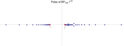
Figure 1: Poles of the diagonal Borel–Padé approximant of order 100 for the perturbative series of $\Gamma(2g)/(2g)-1$. There accumulation of poles in both positive and negative real directions, starting at $s=A\equiv 1/2$ and at $s=-4A=-2$. Note the existence of spurious poles away from the real line: non-stable numerical effects of the Padé method, which move away by choosing different non-diagonal approximants.

III Transseries and Analyticity Conditions

We can now write a trasseries ansatz for our coefficients $c_{\pm}\left(n,g\right)$ appearing in (I).

$$c_{\pm}\left(n,x;\sigma_{i}\right)=\sum_{m_{1},m_{2}=0}^{+\infty}\sigma_{1}^{m_{1}}\sigma_{2}^{m_{2}}\mathrm{e}^{(4m_{2}-m_{1})A\frac{x}{2}}c_{\pm}^{(m_{i})}\left(n,x\right),$$ (24)

where $\sigma_{i}$ are the transseries (or instanton counting) parameters, $A=\frac{1}{2}$ and $c_{\pm}^{(m)}(n,x)$ are perturbative expansions around each non-perturbative sector $(m_{1},m_{2})$: $c_{\pm}^{(0)}(n,x)$ are simply the perturbative expansions (14) found in the previous Section, while the others will generically be

$$c_{\pm}^{(m_{i})}\left(n,x\right)\simeq x^{\beta_{\pm}\left(m_{i}\right)}\sum_{k=0}^{+\infty}x^{-k}\phi_{k}^{(m,\pm)}\left(n\right)n^{\pm 1/4},$$ (25)

where $\beta_{\pm}\left(m\right)$ are numerical factors associated with the type of branch cuts on the Borel plane. In general one is interested in the transseries solution at some particular value of the coupling $x$ (usually real positive), and the parameters $\sigma_{i}$ are fixed by some physical input. Moreover, having a non-zero $\sigma_{2}$ for positive real $x$ would lead to unstable, exponentially enhanced contributions, which physically we know should not be included. Nevertheless, such sectors need to be introduced in order to account for all the analytic properties of the problem at hand, even if in the end, once resummation is performed, the parameter $\sigma_{2}$ gets fixed to zero.

Another important issue is that of resonance Garoufalidis:2010ya ; Aniceto:2011nu ; Schiappa:2013opa ; Upcoming:2015 : for transseries with more than one type of exponential behaviour $\mathrm{e}^{-m_{1}A_{1}-m_{2}A_{2}}$, if there are values $m_{i}$ such that $m_{1}A_{1}+m_{2}A_{2}=0$, a phenomena called resonance occurs. In the case of transseries solutions to non-linear differential equations, it is seen that the associated recursion relations break down at these locations unless we enhance the perturbative expansions $c_{\pm}^{(m)}$ (25) to include other non-perturbative sectors, such as some finite number of powers of $\log(x)$. In the present case we will find resonance when $m_{1}=4m_{2}$, and one can expect a rich structure like the one found for the Painlevé solutions Aniceto:2011nu ; Schiappa:2013opa . For our present case we will limit the study to the transseries contributions up to "two instantons", $m=2$ in (24), and will not reach these structures in our analysis.

Having written the transseries ansatz, we now need to substitute it in the analyticity conditions (3). After some algebra, we can re-write these conditions as

$$2 = \sum_{m_{2},m=0}^{+\infty}\sigma_{1}^{m}\sigma_{2}^{m_{2}}\mathrm{e}^{-A\frac{x}{2}\left(m-4m_{2}\right)}\times$$

$$\times\sum_{r=0}^{\left\lfloor\frac{m}{4\left|\alpha\right|}\right\rfloor}\sigma_{1}^{-4\left|\alpha\right|r}\left(F_{+}^{(m,r)}\left(n,x\right)+F_{-}^{(m,r)}\left(n,x\right)\right),$$

which need to be obeyed for every zero $\alpha=\ell-\frac{1}{4}$, $\ell\in\mathbb{Z}$. Throughout this paper, we focus on the contributions with $m\leq 2$ and $m_{2}=0$. Therefore we will leave the issue of resonance and higher non-perturbative corrections for subsequent work. We briefly note that the last sum in (III) goes up to the integer part $\left\lfloor\frac{m}{4\left|\alpha\right|}\right\rfloor$, which will be non-zero if $m\geq 4\left|\alpha\right|$. For $\alpha_{\ell}<0$ this already happens for $m=1$ and $\alpha_{0}=-1/4$. For $\alpha_{\ell}\geq\alpha_{1}=3/4>0$, the first non-perturbative contribution will be at $m=3$. The case $m=4$ is somewhat special, as both $\alpha_{0}=-1/4$ and $\alpha_{1}=3/4$ return a non-zero sum (for $m\geq 5$ there will be two negative zeroes). It would also be at this point (taking $m_{2}=1$) that we find the first instance of resonance: it is likely that the two effects will mix in the analyticity conditions.

Taking $m_{2}=0$, then the functions $F_{\pm}$ are

$$F_{+}^{(m,r)}\left(n,x\right) = x^{\beta_{+}\left(m-4\left|\alpha\right|r\right)-1/4}\times$$

$$\times\sum_{k=0}^{+\infty}x^{-k}\sum_{n\geq 1}\frac{\phi_{k}^{(m-4\left|\alpha\right|r,+)}\left(n\right)}{n-\alpha}\times$$

$$\times A_{0,1}\left(x,-n\right)\left(\delta_{r,0}\frac{A_{1,1}\left(x,-n\right)}{A_{0,1}\left(x,-n\right)}\alpha+x^{-1}\bar{R}_{r}\left(x,\alpha\right)\right),$$

$$F_{-}^{(m,r)}\left(n,x\right) = x^{\beta_{-}\left(m-4\left|\alpha\right|r\right)-3/4}\times$$

$$\times\sum_{k=0}^{+\infty}x^{-k}\sum_{n\geq 1}\frac{\phi_{k}^{(m-4\left|\alpha\right|r,-)}\left(n\right)}{(n+\alpha)\,n}\times$$

$$\times A_{0,0}\left(x,-n\right)\left(\delta_{r,0}\frac{A_{1,0}\left(x,-n\right)}{A_{0,0}\left(x,-n\right)}\alpha+n\,\bar{R}_{r}\left(x,\alpha\right)\right).$$

We can now solve (III) for each $m$, and this was done for $m=1,2$, in the same manner as for the perturbative series in the previous Section. We found that

$$\beta_{+}\left(1\right)=\frac{3}{4},\,\beta_{-}(1)=\frac{1}{4},\,\beta_{\pm}\left(2\right)=\pm\frac{1}{4},$$ (29)

and also

$$\phi_{k}^{(m,+)}(n) = \sum_{\ell=0}^{k-1}Q_{k,\ell}^{(m,+)}\frac{1}{n^{\ell}}\phi_{1}^{(m,+)}(n),$$

$$\phi_{k}^{(m,-)}(n) = \sum_{\ell=0}^{k}Q_{k,\ell}^{(m,-)}\frac{1}{n^{\ell}}\phi_{0}^{(m,-)}(n),$$ (30)

where

$$\phi_{1}^{(m,+)}(n) = -\mathcal{P}^{(m)}\phi_{0}^{(0,+)}(n),$$

$$\phi_{0}^{(m,+)}(n) = 0,$$ (31)

$$\phi_{0}^{(m,-)}(n) = \mathcal{P}^{(m)}\phi_{0}^{(0,-)}\left(n-1\right).$$

The numerical coefficients $\mathcal{P}^{(m)}$ are also determined:

$$\mathcal{P}^{(1)} = \frac{\overline{\sigma_{1}}\mathrm{e}^{3\pi\mathrm{i}/4}}{2}\frac{\Gamma\left(3/4\right)}{\Gamma(5/4)},$$

$$\mathcal{P}^{(2)} = -\left(\mathcal{P}^{(1)}\right)^{2}.$$ (32)

It is worth noting that these coefficients seem to depend on the transseries parameter, which it is not yet fixed. The value of the transseries parameters can vary with the value of the coupling $x$: even if we fix them to a particular value, when we move on the $x$-plane, these parameters will jump in value when crossing any Stokes line (lines where there are singularities on the Borel plane) – such jump will be governed by the so-called Stokes automorphism. So how can we interpret the numerical values $\mathcal{P}^{(m)}$ if they depend on a parameter which will change its value? In fact, the analyticity conditions are solved in a specific direction on the $x$-plane: the one which was chosen to perform the asymptotic expansions. In this region we will have a specific value $\sigma_{1}\equiv\overline{\sigma_{1}}$, and the $\mathcal{P}^{(m)}$ will be fixed at that position on the $x$-plane.

Once the $c_{\pm}^{(m)}(n,x)$ are determined for $m=0,1,2$, we can write down the corresponding transseries for the cusp anomalous dimension (I). One can write down the full transseries solution corresponding to (24), but for the present we will take $m_{2}=0$. Then

$$\Gamma_{\textrm{cusp}}\left(g,\sigma\right)=2g\left(1+\sum_{m=0}^{+\infty}\sigma^{m}\mathrm{e}^{-mA\frac{x}{2}}\Gamma^{(m)}(x)\right),$$ (33)

where $\sigma\equiv\sigma_{1}\mathcal{P}^{(1)}$, $\Gamma^{(0)}$ was the perturbative contribution previously calculated (II). The two first non-perturbative corrections can be written as ($m=1,2$)

$$\Gamma^{(m)}(x)\simeq x^{-\beta\left(m\right)}\sum_{k=0}^{+\infty}\Gamma_{k}^{(m)}\left(\frac{x}{2}\right)^{-k},$$ (34)

where $\beta\left(m\right)=-\frac{m}{2}$ and the coefficients are

$$\Gamma_{0}^{(m)} = -4\frac{\mathcal{P}^{(m)}}{\left(\mathcal{P}^{(1)}\right)^{m}},$$ (35)

$$\Gamma_{k}^{(m)} = -2^{1-k}\frac{\mathcal{P}^{(m)}}{\left(\mathcal{P}^{(1)}\right)^{m}}\times$$

$$\times\left(\sum_{a=0}^{k}\sum_{s=0}^{a}S_{-}\left(s\right)Q_{k-s,a-s}^{(m,-)}\sum_{r=0}^{a}4^{a+1-r}K_{r}^{(0-)}\right.+$$

$$+\left.\sum_{a=0}^{k-1}\sum_{s=0}^{a}S_{+}\left(s\right)Q_{k-s,a-s}^{(m,+)}K_{a+1}^{(0+)}\right),\>k\geq 1.$$

We have now calculated the perturbative coefficients around the first two non-perturbative sectors. If we analyse the growth of these coefficients, we find the same factorial growth $\Gamma\left(k-1/2\right)$ for $m=0,1$, and the factorial growth $\Gamma\left(k+1/2\right)$ for $m=2$: not only the perturbative series is asymptotic, but so are the non-perturbative ones. Moreover the singularities which lead to these sectors lie on the positive real axis, and thus one cannot properly define a single integration contour on which to perform the resummation of the Borel transform.

Nevertheless, many lessons have been learned by now on the cases of resurgent transseries: if our transseries is resurgent, then there is a way of defining a single non-ambiguous result which properly cancels the imaginary ambiguity at all non-perturbative orders. But in order to use these results from resurgence, we first need to check that our transseries is indeed resurgent.

IV Resurgence and Large-Order

Let us now check that the transseries formed by the asymptotic series $\Gamma^{(m)}$ is indeed resurgent, i.e. that the coefficients $\Gamma_{k}^{(m)},\Gamma_{\ell}^{(m^{\prime})}$ of neighbouring sectors $m,m^{\prime}$ are related. To perform this check we use the coefficients $\Gamma_{k}^{(m)}$ of the asymptotic series (34) and check if their large order behaviour coincides with the large-order relations predicted by resurgence techniques. These are relations between the large order $k\gg 1$ $\Gamma_{k}^{(m)}$ of one sector with the low order coefficients of a nearby sector $\Gamma_{\ell}^{(m^{\prime})}$.

Take the transseries (33); assuming this transseries is resurgent, we can use the so-called alien calculus to determine the discontinuity of each asymptotic series $\Gamma^{(m)}$ across singular directions (or Stokes lines). In our case (given we have taken $m_{2}=0$) we only have one singular direction: the positive real axis $\theta=0$. Resurgence then tells us Aniceto:2011nu that the discontinuity of the perturbative series along this direction is (recall that $A=1/2$)

$$\mathrm{Disc}_{0}\Gamma^{(0)}(x)=-S_{1}\mathrm{e}^{-A\frac{x}{2}}\Gamma^{(1)}-\left(S_{1}\right)^{2}\mathrm{e}^{-2A\frac{x}{2}}\Gamma^{(2)}+\cdots.$$ (37)

There is one unknown constant in the above relation, the Stokes constant $S_{1}$. As we will see, the large order relations will allow us to determine this constant with great accuracy. This step is extremely important as the Stokes constant plays a crucial role in the ambiguity cancelation and resummation.

From the discontinuity, we can use Cauchy’s theorem to determine large-order relations ZinnJustin:1980uk . Schematically, one writes

$$\Gamma^{(0)}(z) = \oint_{\omega=z}\frac{d\omega}{2\pi\mathrm{i}}\frac{\Gamma^{(0)}(\omega)}{\omega-z}$$

$$\simeq \int_{0}^{+\infty}\frac{d\omega}{2\pi\mathrm{i}}\frac{\mathrm{Disc}_{0}\Gamma^{(0)}(\omega)}{\omega-z}+\oint_{\infty}(\cdots).$$

In certain conditions, it can be shown by scaling arguments that the integral at infinity does not contribute Bender:1990pd ; Collins:1977dw . Expanding the r.h.s for large $z$, using the resurgence relation for the discontinuity, and finally comparing equal powers of $z$ for the expansions in both sides of the equation, we arrive at the relation

$$\Gamma_{k}^{(0)} \simeq -\frac{S_{1}\mathcal{P}^{(1)}}{2\pi\mathrm{i}}\sum_{h=0}^{+\infty}\Gamma_{h}^{(1)}\frac{\Gamma\left(k-\frac{1}{2}-h\right)}{A^{k-\frac{1}{2}-h}}-$$

$$-\frac{\left(S_{1}\mathcal{P}^{(1)}\right)^{2}}{2\pi\mathrm{i}}\sum_{h=0}^{+\infty}\Gamma_{h}^{(1)}\frac{\Gamma\left(k-1-h\right)}{(2A)^{k-1-h}},\>k\gg 1.$$

This formula states that if resurgence is expected, then the large $k$ behaviour of the perturbative series is dictated by the coefficients of the first non-perturbative sector, and then, more exponentially suppressed ($2^{-k}$), the coefficients of the second non-perturbative sector appear, and so on. The proportionality constant is once again the Stokes constant $S_{1}$. Taking the ratio (which removes the dependence on the yet unknown Stokes constant) of two consecutive coefficients, and assuming $k\gg 1$, we have a series (asymptotic again)

$$\frac{\Gamma_{k}^{(0)}}{\Gamma_{k+1}^{(0)}}\frac{k}{A}\simeq\sum_{h=0}^{+\infty}c_{h}\,k^{-h},$$ (40)

where the coefficients $c_{h}$ can be predicted from the original large order relation (IV). The first coefficients are

$$c_{0}=1;\>c_{1}=\frac{1}{2};\>c_{2}=\frac{1}{4}+A\frac{\Gamma_{1}^{(1)}}{\Gamma_{0}^{(1)}};\>\cdots.$$ (41)

We can now check the convergence of $\Gamma_{k}^{(0)}$ to the coefficients $c_{h}$ by successively removing the previous coefficient from the ratio. For example to check the convergence to the coefficient $c_{2}$ we analyse

$$\left(\left(\frac{\Gamma_{k}^{(0)}}{\Gamma_{k+1}^{(0)}}\frac{k}{A}-c_{0}\right)k-c_{1}\right)k\rightarrow c_{2}+O\left(k^{-1}\right).$$ (42)

In Figure 2 we present the convergence to coefficient $c_{10}$. In order for this convergence to be correct, all of the previous coefficients need to be correct to a very high accuracy, since factorial errors propagate rapidly. In this figure, the original ratio (in red) is shown, together with two related Richardson transforms which speed the convergence of this series in $1/n$ (see Marino:2007te ; Garoufalidis:2010ya ). The error between the numerically calculated coefficient (via Richardson transforms) and the predicted result from the large-order formula is of order $10^{-7}$.

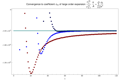
Figure 2: Convergence of the large order ratio of perturbative coefficients to the predicted result related to the first non-perturbative sector. In red is shown the original ratio, and in blue the corresponding Richardson transforms of order 2 (light blue) and 6 (dark blue). In light green the predicted value for the coefficient $c_{10}$ is shown.

If instead of dealing with the ratio of coefficients we analyse the following

$$\frac{2\pi\,A^{k-\frac{1}{2}}\,\Gamma_{k}^{(0)}}{\Gamma\left(k-\frac{1}{2}\right)\Gamma_{0}^{(1)}} \simeq \mathrm{i}S_{1}\mathcal{P}^{(1)}\sum_{h=0}^{+\infty}\frac{\Gamma_{h}^{(1)}}{\Gamma_{0}^{(1)}}\frac{\Gamma\left(k-\frac{1}{2}-h\right)}{\Gamma\left(k-\frac{1}{2}\right)}A^{h}$$ (43)

$$\sim \mathrm{i}S_{1}\mathcal{P}^{(1)}+O\left(k^{-1}\right),$$

we directly obtain a convergence to the unknown Stokes constant. In Figure 3 this convergence is shown, with both the original series and a related Richardson transform. The increase in convergence speed from the Richardson interpolation method allows us to determine the Stokes constant to a very high accuracy. Up to an error of $10^{-23}$ we find

$$\mathrm{i}S_{1}\mathcal{P}^{(1)}=\frac{1}{2}\frac{\Gamma\left(3/4\right)}{\Gamma(5/4)}.$$ (44)

The same ideas were repeated for the asymptotic series of $\Gamma^{(1)}$, whose large order will be directly related to coefficients of $\Gamma^{(2)}$, finding that resurgence predictions also worked in this case. Note that unlike the previous cases, the large-order behaviour of $\Gamma^{(2)}$ is dictated not only by $\Gamma^{(3)}$ but also by $\Gamma^{(1)}$ (the two nearest singularities on the Borel plane will be equally distant from the origin, at $s=\pm A$). We conclude that indeed the transseries for the cusp anomalous dimension is resurgent, and thus we can apply the methods of ambiguity cancelation known to exist for resurgent transseries.

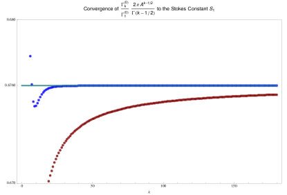
Figure 3: Convergence of the perturbative coefficients to the Stokes constant. In red the original series is shown, and in blue the second Richardson transform with increased convergence. In dark green the calculated value for the Stokes constant is shown.

V Ambiguity Cancelation and Interpolation

The next two questions which follow are: if our transseries is resurgent, can we use this knowledge to write a non-ambiguous result? And if this is possible, can we then interpolate from the strong coupling asymptotic expansion to small coupling?

The answer to the first question is simply yes. The fact that we have a resurgent transseries directly tells us how to obtain a non-ambiguous result even when resumming in directions which are non-Borel summable, i.e., along Stokes lines.

In order to verify the ambiguity cancelation it is sufficient to check that the imaginary part of the resummed lateral transseries cancels to higher and higher orders. The ambiguity coming from the perturbative series, i.e. the imaginary contribution from performing a lateral resummation, is of order $\mathrm{e}^{-A\,4\pi g}$ for each value of the coupling $g$. This is exactly the order at which the first non-perturbative sector starts contributing. In fact, if we add the two with the proper choice of parameter $\sigma$ in (7) we can see that the newfound imaginary part will now be of order $\mathrm{e}^{-2A\,4\pi g}$ - the order of the second non-perturbative sector. In order to see this cancelation, and to determine the value of the parameter $\sigma=\sigma_{1}\mathcal{P}^{(1)}$ which brings about the cancelation, we first need to resum our asymptotic series.

The method for resumming our series is the so-called Écalle-Borel–Padé resummation method. It consists in calculating the Borel transforms for each sector $\mathcal{B}\left[\Gamma^{(m)}\right](s)$, then determining a Padé approximant for each Borel transform, and subsequently perform a lateral Borel resummation (we have chosen $\mathcal{S}_{+}$ as in (10)) for different values of the coupling $0.1\leq g\leq 4$ in order to obtain a resummed result for the full transseries for general values of $g$. The imaginary part of the transseries for the cusp

$$\frac{\mathcal{S}_{+}\Gamma}{2g}-1=\mathcal{S}_{+}\Gamma^{(0)}+\sigma\,\mathrm{e}^{-\frac{1}{2}4\pi g}\mathcal{S}_{+}\Gamma^{(1)}+\sigma^{2}\,\mathrm{e}^{-4\pi g}\mathcal{S}_{+}\Gamma^{(2)}+\cdots$$ (45)

is given by (12). In Figure 4 the order $10^{-\alpha}$ of the imaginary part can be seen if we only include $\mathcal{S}_{+}\Gamma^{(0)}$ (dark brown), or if we include both perturbative and first non-perturbative contributions (light brown), and finally if we include all calculated contributions (up to second order, in purple). The cancelation is shown for a range of values of the coupling, ranging from weak to strong coupling. For example for $g=1.5$ if we include only the perturbative part, the imaginary ambiguity is of order $10^{-5}$. Including the first non-perturbative sector cancels this imaginary part to $10^{-10}$. Including all three sectors cancels the imaginary part up to 16 decimal places. The value of the transseries parameter used was

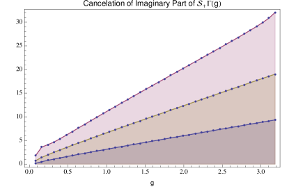
Figure 4: Order of magnitude $10^{-\alpha}$ (where $\alpha$ is shown on the y-axis) of the imaginary part of the transseries for the cusp anomalous dimension, when one adds only the perturbative series (dark brown), if one adds also the first non-perturbative correction (light brown) and if one takes all three calculated contributions (light purple).

$$\sigma_{0}=-\left(1+\mathrm{i}\right)\frac{\mathrm{i}S_{1}\mathcal{P}^{(1)}}{2}=\frac{1}{2\sqrt{2}}\mathrm{e^{-3\pi\mathrm{i}/4}}\frac{\Gamma\left(3/4\right)}{\Gamma\left(5/4\right)},$$ (46)

with the Stokes constant given by (44). This is in complete agreement with the proportionality constant appearing in front of the non-perturbative corrections in Basso:2009gh .

We are now ready to answer the second question posed in this Section: once we have managed to write down a real unambiguous transseries result, given by (I) with the parameter $\sigma_{0}$ determined in (46), can we use this result to interpolate between strong and weak coupling? In Figure 5 we show the truncated asymptotic series result in a dashed green line: this result is accurate at strong coupling, but diverges for weak coupling. In blue we plotted the weak coupling expansion for the cusp anomalous dimension as determined (up to 7 loop order) by Beisert:2006ez . Naturally this result diverges for large values of the coupling. In red we show the resummed result including the perturbative series and the first two non-perturbative sectors. We see clearly that the red dots follow both the strong and weak regime closely, starting to diverge for $g<0.2$. In order to obtain more accurate results after this point, we would need to include the next non-perturbative order.

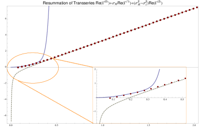
Figure 5: Resummation of the transseries result for different values of the coupling, shown in red. For large coupling the behaviour is dictated by the perturbative series alone, as shown by the dashed line – the truncated summation of the perturbative expansion $\Gamma^{(0)}$, which diverges for small g. In this regime another line is shown in blue, corresponding to the small coupling expansion (up to 7 loops) of the cusp anomalous dimension. The red dots interpolate between these two regimes, starting to diverge around value $g=0.2$.

In summary, once we have established resurgence of the transseries, we are able to write down an unambiguous result, and use that same result to reach values of the coupling as small as $g=0.2$. Moreover, the information encoded in the transseries solution for the cusp anomalous dimension goes beyond the strong/weak interpolation for positive real values of the coupling. The resummation can be performed for $g\in\mathbb{C}$: one can obtain a solution for any value of coupling, having in mind that to reach certain values one might have to cross a Stokes line and the transseries goes through a so-called Stokes transition (in a Stokes transition the transseries parameters will jump in value, and this jump is dictated by the Stokes constants and can be calculated from resurgence techniques). In other words, the transseries solution encodes the analytic properties of the cusp anomalous dimension as a function of the coupling.

Another extremely insightful example of how the transseries encoded the analytic properties of the observable was recently achieved in the context of matrix models Couso-Santamaria:2015wga , where from a large $N$ asymptotic expansion, resurgence and resummation techniques allowed the authors to reach not only finite values of the rank $N$, but they were also able to analytically continue their results to any complex value of $N$, once Stokes phenomena were taken into account.

VI Conclusions/Outlook

In this work we presented a thorough analysis of the resurgent properties of the cusp anomalous dimension’s strong coupling expansion. When analysing the perturbative series we found that there are two types of singularities on the Borel plane in both the positive and negative real axis. These need to be taken into account in order to fully solve the analyticity conditions coming from the BES equations. Nevertheless their physical interpretation has not yet been addressed. The non-perturbative behaviour associated with singularities at $s=nA$ (on the positive real axis), were seen to be directly linked to the mass gap of the $O(6)$ $\sigma$-model at least for $n=1$ Basso:2009gh . The singularities at $s=-4nA$ are much more suppressed and as such haven’t been addressed, but some questions can be immediately raised: does the same feature appear for the energy density of the $O(6)$ model? Does the relation between scaling function and energy density hold for higher exponentially suppressed contributions? Since the two types of non-perturbative phenomena are collinear, will we witness resonance?

For the aims of the current paper we used a transseries ansatz for the cusp anomalous dimension which did not include the second type of non-perturbative phenomena, as we only studied the solution up to $n=2$ in the non-perturbative order. Nevertheless this was enough to check the resurgent properties of the strong coupling expansion, with the large-order relations predicted by resurgence accurately solving the large order behaviour of the perturbative expansion and first non-perturbative order.

In our case we could determine the asymptotic expansions around the non-perturbative sectors via the BES equation, and use these to check the resurgence of the transseries. In cases when only perturbation theory is known, one can go the opposite way and use the predictions of resurgence to determine the coefficients of the expansions around the non-perturbative sectors.

Knowing that the transeries proposed is indeed resurgent we then proceeded to determine the resummed transseries, using a lateral resummation procedure. This naturally introduces an imaginary ambiguity, which can then be seen to cancel given the proper choice of the transseries parameter: using the methods of median resummation Aniceto:2013fka we determined the transseries parameter to be the one proposed in Basso:2009gh .

Finally the resummation procedure can be done for different values of the coupling, and we showed that including up to second order non-perturbative effects, we could systematically obtain accurate results for the cusp anomalous dimension all the way from strong coupling up to $g\simeq 0.2$. Moreover we can perform the resummation for any values of the coupling, as long as we take into consideration the Stokes phenomena occurring when we analytically continue our results across Stokes lines.

This work is an example in the use and elegance of the resurgence techniques. Knowing the perturbative asymptotic expansion of an observable in some regime, we can determine the non-perturbative corrections via large order relations, and upgrade the solution to a transseries. We can then use resummation methods such as Écalle-Borel–Padé to obtain a resummed solution for any value of the coupling (using resurgence techniques to analytically continue the solution across Stokes lines). This resummed transseries encodes the analytic properties of our observable as a function of the coupling.

Other open questions still to be addressed are whether one can use a transseries ansatz for the auxiliary function in the BES equation, and through this find an equivalent approach to determining the coefficients $\Gamma_{k}^{(m)}$ to the one used in Basso:2007wd ; Basso:2009gh . Also, it remains to be understood how these results translate to the problem of the scaling function $\epsilon(g,j)$ and the energy density of the $O(6)$ $\sigma$-model. The first question is if one can find a full transseries in these cases. If so, will we have the same type of singularities? Finally, in these two cases we have two parameters $g,j$ and it would be important to understand how the different regimes dictated by these parameters appear in the resurgent context.

Appendix A Asymptotic Expansions

In order to write down the asymptotic expressions appearing in the main text, we need first to define the following four asymptotic expansions

$$A_{0,0}\left(x,\alpha\right) = \sum_{s=0}^{+\infty}\frac{\Gamma\left(\frac{3}{4}+s\right)\Gamma\left(-\frac{1}{4}+s\right)}{\Gamma\left(-\frac{1}{4}\right)\,s!\,\left(x\,\alpha\right)^{s}},$$ (47)

$$A_{0,1}\left(x,\alpha\right) = \sum_{s=0}^{+\infty}\frac{\Gamma\left(\frac{1}{4}+s\right)\Gamma\left(\frac{5}{4}+s\right)}{\Gamma\left(\frac{1}{4}\right)\,s!\,\left(x\,\alpha\right)^{s}},$$ (48)

$$A_{1,0}\left(x,\alpha\right) = \sum_{s=0}^{+\infty}\frac{\Gamma\left(\frac{3}{4}+s\right)^{2}}{\Gamma\left(\frac{3}{4}\right)\,s!\,\left(x\,\alpha\right)^{s}},$$ (49)

$$A_{1,1}\left(x,\alpha\right) = \sum_{s=0}^{+\infty}\frac{\Gamma\left(\frac{1}{4}+s\right)^{2}}{\Gamma\left(\frac{1}{4}\right)\,s!\,\left(x\,\alpha\right)^{s}}.$$ (50)

In all the expressions in this appendix we assume $\alpha\neq 0$. The functions $U_{n}^{\pm}\left(x\right),\,n=0,1$ have been defined in Basso:2009gh in terms of Whittaker functions of the second kind. For the purposes of this paper however, we are only interested in their asymptotic expansions for large $x$, which are:

$$U_{0}^{+}\left(\frac{nx}{2}\right) \simeq \left(nx\right)^{-5/4}A_{0,1}\left(x,-n\right),$$

$$U_{0}^{-}\left(\frac{nx}{2}\right) \simeq \left(nx\right)^{-3/4}A_{0,0}\left(x,-n\right),$$ (51)

$$U_{1}^{+}\left(\frac{nx}{2}\right) \simeq \frac{1}{2}\left(nx\right)^{-1/4}A_{1,1}\left(x,-n\right),$$

$$U_{1}^{-}\left(\frac{nx}{2}\right) \simeq \frac{1}{2}\left(nx\right)^{-3/4}A_{1,0}\left(x,-n\right).$$

Note that even from these asymptotic expansions it is not difficult to see that these functions have a cut on the negative real axis. The other functions of interest appearing in the main text are $V_{n}\left(x\right),\,n=0,1$. Again, in Basso:2009gh these are entire functions which were written in terms of Whittaker functions of the first kind, but for our purposes we are only interested in their asymptotic expansions. More specifically we will only need the asymptotic expansion of their ratio:

$$2r\left(\alpha\right)\equiv 2\frac{V_{1}\left(\frac{\alpha x}{2}\right)}{V_{0}\left(\frac{\alpha x}{2}\right)}.$$ (52)

The asymptotic expansion of this ratio for large $x$ depends on the sign of $\alpha$. For $\alpha=\left|\alpha\right|>0$

$$2r\left(\left|\alpha\right|\right)\simeq\sum_{k=0}^{+\infty}(-1)^{k}\mathrm{e}^{-k\left|\alpha\right|x}\mathrm{e}^{5\pi\mathrm{i}k/4}\left(\left|\alpha\right|x\right)^{-k/2}R_{k}\left(x,\left|\alpha\right|\right)$$ (53)

where

$$R_{0}\left(x,\left|\alpha\right|\right) = \frac{A_{1,0}\left(x,\left|\alpha\right|\right)}{A_{0,0}\left(x,\left|\alpha\right|\right)},$$ (54)

$$R_{k}\left(x,\left|\alpha\right|\right) = \left(R_{0}\left(x,\left|\alpha\right|\right)+\left|\alpha\right|x\frac{A_{1,1}\left(x,-\left|\alpha\right|\right)}{A_{0,1}\left(x,-\left|\alpha\right|\right)}\right)\times$$

$$\qquad\qquad\qquad\qquad\times\left(\frac{A_{0,1}\left(x,-\left|\alpha\right|\right)}{A_{0,0}\left(x,\left|\alpha\right|\right)}\right)^{k}.$$

For $\alpha=-\left|\alpha\right|<0$ we then have

$$2r\left(-\left|\alpha\right|\right)\simeq\sum_{k=0}^{+\infty}(-1)^{k}\mathrm{e}^{-k\left|\alpha\right|x}\mathrm{e}^{3\pi\mathrm{i}k/4}\left(\left|\alpha\right|x\right)^{k/2}\widetilde{R}_{k}\left(x,\left|\alpha\right|\right)$$ (55)

where

$$\widetilde{R}_{0}\left(x,\left|\alpha\right|\right) = x\left|\alpha\right|\frac{A_{1,1}\left(x,\left|\alpha\right|\right)}{A_{0,1}\left(x,\left|\alpha\right|\right)},$$ (56)

$$\widetilde{R}_{k}\left(x,\left|\alpha\right|\right) = \left(\widetilde{R}_{0}\left(x,\left|\alpha\right|\right)-\frac{A_{1,0}\left(x,-\left|\alpha\right|\right)}{A_{0,0}\left(x,-\left|\alpha\right|\right)}\right)\times$$

$$\qquad\qquad\qquad\qquad\times\left(\frac{A_{0,0}\left(x,-\left|\alpha\right|\right)}{A_{0,1}\left(x,\left|\alpha\right|\right)}\right)^{k}.$$

In Section III when solving the analyticity conditions, some particular combinations of the asymptotic expansions $A_{i,j}\left(x,\alpha\right)$ repeatedly appeared. These were

$$M_{0}^{(+)}(x) \equiv \frac{A_{0,1}\left(x,-n\right)}{x}\times$$ (57)

$$\qquad\times\left(\frac{A_{1,1}(x,-n)}{A_{0,1}\left(x,-n\right)}\left|\alpha\right|x+\frac{A_{1,0}\left(x,\left|\alpha\right|\right)}{A_{0,0}\left(x,\left|\alpha\right|\right)}\right)$$

$$\simeq \left|\alpha\right|\Gamma\left(\frac{5}{4}\right)\sum_{r=0}^{+\infty}x^{-r}\sum_{\ell=0}^{r}\frac{M_{r,\ell}^{(0,+)}}{n^{\ell}\left|\alpha\right|^{r-\ell}},$$

$$M_{1}^{(+)}(x) \equiv \frac{A_{0,0}\left(x,-n\right)}{xn\left(n+\left|\alpha\right|\right)}\times$$ (58)

$$\qquad\times\left(\frac{A_{1,0}(x,-n)}{A_{0,0}\left(x,-n\right)}\left|\alpha\right|+n\frac{A_{1,0}\left(x,\left|\alpha\right|\right)}{A_{0,0}\left(x,\left|\alpha\right|\right)}\right)$$

$$\simeq \frac{1}{n}\Gamma\left(\frac{3}{4}\right)\sum_{r=0}^{+\infty}x^{-r-1}\sum_{\ell=0}^{r}\frac{M_{r,\ell}^{(1,+)}}{n^{\ell}\left|\alpha\right|^{r-\ell}},$$

$$M_{0}^{(-)}(x) \equiv \frac{A_{0,1}\left(x,-n\right)}{(n+\left|\alpha\right|)}\left|\alpha\right|\times$$ (59)

$$\qquad\times\left(-\frac{A_{1,1}(x,-n)}{A_{0,1}\left(x,-n\right)}+\frac{A_{1,1}\left(x,\left|\alpha\right|\right)}{A_{0,1}\left(x,\left|\alpha\right|\right)}\right)$$

$$\simeq \frac{1}{n}\Gamma\left(\frac{5}{4}\right)\sum_{r=0}^{+\infty}x^{-r-1}\sum_{\ell=0}^{r}\frac{M_{r,\ell}^{(0,-)}}{n^{\ell}\left|\alpha\right|^{r-\ell}},$$

$$M_{1}^{(-)}(x) \equiv \frac{A_{0,0}\left(x,-n\right)}{xn}\left|\alpha\right|\times$$ (60)

$$\qquad\times\left(-\frac{A_{1,0}(x,-n)}{A_{0,0}\left(x,-n\right)}+xn\frac{A_{1,1}\left(x,\left|\alpha\right|\right)}{A_{0,1}\left(x,\left|\alpha\right|\right)}\right)$$

$$\simeq \left|\alpha\right|\Gamma\left(\frac{3}{4}\right)\sum_{r=0}^{+\infty}x^{-r}\sum_{\ell=0}^{r}\frac{M_{r,\ell}^{(1,-)}}{n^{\ell}\left|\alpha\right|^{r-\ell}}.$$

Appendix B Relations Between Sums

Given the two fundamental objects $\phi_{0}^{(0,\pm)}\left(n\right)$ independent of the coupling $x=8\pi g$, appearing in the transseries of the coefficients $c_{\pm}\left(n,x\right)$ in (24), these can easily be determined from analyticity conditions to be

$$\phi_{0}^{(0,+)}(n) = 2\frac{\Gamma\left(n-\frac{3}{4}+1\right)}{n!\,\Gamma\left(\frac{1}{4}\right)^{2}},$$ (61)

$$\phi_{0}^{(0,-)}\left(n\right) = \frac{\Gamma\left(n-\frac{1}{4}+1\right)}{2\,n!\,\Gamma\left(\frac{3}{4}\right)^{2}}.$$ (62)

With these definitions we calcuate the following sums for $m\geq 1$

$$K_{m}^{(0,+)} \equiv -\Gamma\left(\frac{5}{4}\right)\sum_{n\geq 1}\frac{\phi_{0}^{(0,+)}(n)}{n^{m}}$$ (63)

$$= -\frac{1}{8}\,_{m+2}F_{m+1}\left(\mathbf{a}^{+},\mathbf{b};1\right),$$

$$K_{m}^{(0,-)} \equiv -\Gamma\left(\frac{3}{4}\right)\sum_{n\geq 1}\frac{\phi_{0}^{(0,-)}(n)}{n^{m}}$$ (64)

$$= -\frac{3}{8}\,_{m+2}F_{m+1}\left(\mathbf{a}^{-},\mathbf{b};1\right),$$

where $\,{}_{p+1}F_{p}$ is a generalized hypergeometric function, $\mathbf{a}^{\pm}$ are vectors with $m+2$ entries: $\mathbf{a^{+}}=\left(1,\cdots,1,5/4\right)$ and $\mathbf{a^{-}}=\left(1,\cdots,1,7/4\right)$, whereas $\mathbf{b}=\left(2,\cdots,2\right)$ is a vector with $m+1$ entries. Defining also $K_{0}^{(0,\pm)}\equiv 1/2$, one can easily see that

$$\Gamma\left(\frac{5}{4}\right)\sum_{n\geq 1}\frac{\phi_{0}^{(0,+)}(n)\left|\alpha\right|}{(n-\left|\alpha\right|)n^{m}} = \sum_{\ell=0}^{m}\frac{K_{\ell}^{(0,+)}}{\left|\alpha\right|^{m-\ell}},$$

$$\Gamma\left(\frac{3}{4}\right)\sum_{n\geq 1}\frac{\phi_{0}^{(0,-)}(n)\left|\alpha\right|}{(n-\left|\alpha\right|)n^{m}} = \sum_{\ell=0}^{m}\frac{K_{\ell}^{(0,-)}}{\left|\alpha\right|^{m-\ell}}.$$ (65)

In all the expressions in this Appendix we assume $\alpha_{\ell}=\ell-1/4$, for $\ell\in\mathbb{Z}$. Other useful identities of $\phi_{0}^{(0,-)}(n)$ are

$$\sum_{n\geq 1}\frac{\phi_{0}^{(0,-)}(n-1)}{n-\left|\alpha_{\ell}\right|}=0,\>\ell\leq-1,$$ (66)

$$\Gamma\left(\frac{3}{4}\right)\sum_{n\geq 1}\frac{\phi_{0}^{(0,-)}(n-1)}{\left(n-\left|\alpha_{\ell}\right|\right)n^{m}} =$$

$$=-\sum_{s=0}^{m-1}\frac{1}{\left|\alpha_{\ell}\right|^{m-s}}\sum_{r=0}^{s}\frac{K_{r}^{(0,-)}}{\left|\alpha_{0}\right|^{s-r+1}},\>m,-\ell\geq 1,$$

$$\Gamma\left(\frac{3}{4}\right)\sum_{n\geq 1}\frac{\phi_{0}^{(0,-)}(n-1)}{n^{m}}=\sum_{\ell=0}^{m-1}\frac{K_{\ell}^{(0,-)}}{\left|\alpha_{0}\right|^{m-\ell}},\>m\geq 1,$$ (68)

$$\Gamma\left(\frac{3}{4}\right)\left|\alpha_{0}\right|\sum_{n\geq 1}\frac{\phi_{0}^{(0,-)}(n-1)}{(n-\left|\alpha_{0}\right|)n^{m}}=\sum_{\ell=0}^{m}\frac{K_{\ell}^{(1,-)}}{\left|\alpha_{0}\right|^{m-\ell}},\>m\geq 0,$$ (69)

where $K_{0}^{(1,-)}=\pi/(4\sqrt{2})$ and for $\ell\geq 1$ $K_{\ell}^{(1,-)}=(-1)\sum_{a=0}^{\ell-1}4^{\ell-a}K_{a}^{(0,-)}$. Useful identities of $\phi_{0}^{(0,+)}(n)$ are

$$\Gamma\left(\frac{5}{4}\right)\left|\alpha_{0}\right|\sum_{n\geq 1}\frac{\phi_{0}^{(0,+)}(n)}{(n+\left|\alpha_{0}\right|)n^{m}}=-\sum_{\ell=0}^{m}\left(-4\right)^{m-\ell}K_{\ell}^{(1,+)},$$ (70)

where $K_{0}^{(1,+)}=\frac{1}{2}-\frac{\pi}{4\sqrt{2}}$ and $K_{\ell}^{(1,+)}=K_{\ell}^{(0,+)}$ for $\ell\geq 1$.

References

- (1) A. M. Polyakov Nucl.Phys. B164 (1980) 171–188.
- (2) A. V. Belitsky, A. S. Gorsky, and G. P. Korchemsky Nucl. Phys. B748 (2006) 24–59, hep-th/0601112.
- (3) L. F. Alday and J. M. Maldacena JHEP 0711 (2007) 019, arXiv:0708.0672 [hep-th].
- (4) L. Freyhult, A. Rej, and M. Staudacher J. Stat. Mech. 0807 (2008) P07015, 0712.2743.
- (5) S. Frolov, A. Tirziu, and A. A. Tseytlin Nucl. Phys. B766 (2007) 232–245, hep-th/0611269.
- (6) G. Korchemsky and A. Radyushkin Nucl.Phys. B283 (1987) 342–364.
- (7) G. Korchemsky Mod.Phys.Lett. A4 (1989) 1257–1276.
- (8) Z. Bern, M. Czakon, L. J. Dixon, D. A. Kosower, and V. A. Smirnov Phys.Rev. D75 (2007) 085010, arXiv:hep-th/0610248 [hep-th].
- (9) F. Cachazo, M. Spradlin, and A. Volovich Phys.Rev. D75 (2007) 105011, arXiv:hep-th/0612309 [hep-th].
- (10) J. M. Maldacena Adv. Theor. Math. Phys. 2 (1998) 231–252, hep-th/9711200.
- (11) S. S. Gubser, I. R. Klebanov, and A. M. Polyakov Phys. Lett. B428 (1998) 105–114, hep-th/9802109.
- (12) S. Frolov and A. A. Tseytlin JHEP 06 (2002) 007, hep-th/0204226v5.
- (13) G. Arutyunov, S. Frolov, and M. Staudacher JHEP 10 (2004) 016, hep-th/0406256.
- (14) M. Staudacher JHEP 05 (2005) 054, hep-th/0412188.
- (15) N. Beisert and M. Staudacher Nucl. Phys. B727 (2005) 1–62, hep-th/0504190.
- (16) B. Eden and M. Staudacher J.Stat.Mech. 0611 (2006) P11014, arXiv:hep-th/0603157 [hep-th].
- (17) N. Beisert, B. Eden, and M. Staudacher J. Stat. Mech. 01 (2007) P021, hep-th/0610251.
- (18) A. Belitsky Phys.Lett. B643 (2006) 354–361, arXiv:hep-th/0609068 [hep-th].
- (19) B. Basso and G. Korchemsky Nucl.Phys. B807 (2009) 397–423, arXiv:0805.4194 [hep-th].
- (20) M. Benna, S. Benvenuti, I. Klebanov, and A. Scardicchio Phys. Rev. Lett. 98 (2007) 131603, hep-th/0611135.
- (21) L. F. Alday, G. Arutyunov, M. Benna, B. Eden, and I. Klebanov JHEP 0704 (2007) 082, arXiv:hep-th/0702028 [HEP-TH].
- (22) I. Kostov, D. Serban, and D. Volin Nucl. Phys. B789 (2008) 413–451, hep-th/0703031.
- (23) M. Beccaria, G. F. D. Angelis, and V. Forini JHEP 04 (2007) 066, hep-th/0703131.
- (24) B. Basso, G. Korchemsky, and J. Kotanski Phys.Rev.Lett. 100 (2008) 091601, arXiv:0708.3933 [hep-th].
- (25) I. Kostov, D. Serban, and D. Volin JHEP 0808 (2008) 101, arXiv:0801.2542 [hep-th].
- (26) P. Hasenfratz, M. Maggiore, and F. Niedermayer Phys.Lett. B245 (1990) 522–528.
- (27) P. Hasenfratz and F. Niedermayer Phys.Lett. B245 (1990) 529–532.
- (28) B. Basso and G. P. Korchemsky J. Phys. A42 (2009) 254005, 0901.4945.
- (29) Z. Bajnok, J. Balog, B. Basso, G. Korchemsky, and L. Palla Nucl.Phys. B811 (2009) 438–462, arXiv:0809.4952 [hep-th].
- (30) D. Volin Phys.Rev. D81 (2010) 105008, arXiv:0904.2744 [hep-th].
- (31) A. Olde Daalhuis Proceedings of the Royal Society of London A: Mathematical, Physical and Engineering Sciences 461 no. 2062, (2005) 3005–3021.
- (32) S. Garoufalidis, A. Its, A. Kapaev, and M. Mariño Int. Math. Res. Notices 2012 (2012) 561, arXiv:1002.3634 [math.CA].
- (33) I. Aniceto, R. Schiappa, and M. Vonk Commun. Num. Theor. Phys. 6 (2012) 339, arXiv:1106.5922 [hep-th].
- (34) R. Schiappa and R. Vaz Commun.Math.Phys. 330 (2014) 655–721, arXiv:1302.5138 [hep-th].
- (35) C. M. Bender and T. T. Wu Phys. Rev. 184 (1969) 1231.
- (36) C. M. Bender and T. Wu Phys. Rev. D7 (1973) 1620.
- (37) F. Dyson Phys.Rev. 85 (1952) 631–632.
- (38) J. Zinn-Justin Phys.Rept. 70 (1981) 109.
- (39) M. Beneke Phys. Rept. 317 (1999) 1, arXiv:hep-ph/9807443 [hep-ph].
- (40) E. Bogomolny Phys. Lett. B91 (1980) 431.
- (41) J. Zinn-Justin Nucl.Phys. B192 (1981) 125–140.
- (42) J. Zinn-Justin Nucl.Phys. B218 (1983) 333–348.
- (43) G. V. Dunne and M. Ünsal Phys.Rev. D89 no. 4, (2014) 041701, arXiv:1306.4405 [hep-th].
- (44) G. Başar, G. V. Dunne, and M. Ünsal JHEP 1310 (2013) 041, arXiv:1308.1108 [hep-th].
- (45) G. V. Dunne and M. Unsal Phys.Rev. D89 no. 10, (2014) 105009, arXiv:1401.5202 [hep-th].
- (46) F. David Nucl.Phys. B348 (1991) 507–524.
- (47) F. David Phys.Lett. B302 (1993) 403–410, arXiv:hep-th/9212106 [hep-th].
- (48) M. Mariño JHEP 0803 (2008) 060, arXiv:hep-th/0612127 [hep-th].
- (49) M. Mariño, R. Schiappa, and M. Weiss Commun. Num. Theor. Phys. 2 (2008) 349, arXiv:0711.1954 [hep-th].
- (50) M. Mariño JHEP 0812 (2008) 114, arXiv:0805.3033 [hep-th].
- (51) M. Mariño, R. Schiappa, and M. Weiss J. Math. Phys. 50 (2009) 052301, arXiv:0809.2619 [hep-th].
- (52) S. Pasquetti and R. Schiappa Annales Henri Poincaré 11 (2010) 351, arXiv:0907.4082 [hep-th].
- (53) R. Couso-Santamaría, R. Schiappa, and R. Vaz Annals Phys. 356 (2015) 1–28, arXiv:1501.01007 [hep-th].
- (54) G. V. Dunne and M. Ünsal JHEP 1211 (2012) 170, arXiv:1210.2423 [hep-th].
- (55) G. V. Dunne and M. Ünsal Phys. Rev. D87 (2013) 025015, arXiv:1210.3646 [hep-th].
- (56) A. Cherman, D. Dorigoni, G. V. Dunne, and M. Ünsal Phys.Rev.Lett. 112 (2014) 021601, arXiv:1308.0127 [hep-th].
- (57) I. Aniceto, J. G. Russo, and R. Schiappa JHEP 1503 (2015) 172, arXiv:1410.5834 [hep-th].
- (58) M. Shifman J.Exp.Theor.Phys. 120 no. 3, (2015) 386–398, arXiv:1411.4004 [hep-th].
- (59) G. Başar and G. V. Dunne JHEP 1502 (2015) 160, arXiv:1501.05671 [hep-th].
- (60) G. V. Dunne and M. Ünsal arXiv:1505.07803 [hep-th].
- (61) R. Couso-Santamaría, J. D. Edelstein, R. Schiappa, and M. Vonk Annales Henri Poincaré, in press .
- (62) R. Couso-Santamaría, J. D. Edelstein, R. Schiappa, and M. Vonk Commun.Math.Phys. 338 no. 1, (2015) 285–346, arXiv:1407.4821 [hep-th].
- (63) A. Grassi, M. Marino, and S. Zakany JHEP 1505 (2015) 038, arXiv:1405.4214 [hep-th].
- (64) D. Sauzin arXiv:1405.0356 [math.DS].
- (65) D. Dorigoni arXiv:1411.3585 [hep-th].
- (66) I. Aniceto, G. Başar, and R. Schiappa upcoming (2015) .
- (67) C. Bender and S. Orszag McGraw-Hill (1978) .
- (68) I. Aniceto and R. Schiappa Commun.Math.Phys. 335 no. 1, (2015) 183–245, arXiv:1308.1115 [hep-th].
- (69) M. P. Heller and M. Spalinski arXiv:1503.07514 [hep-th].
- (70) Y. Hatsuda and K. Okuyama arXiv:1505.07460 [hep-th].
- (71) J. C. Collins and D. E. Soper Annals Phys. 112 (1978) 209–234.