Quark production in heavy ion collisions:
Formalism and boost invariant
fermionic light-cone mode functions

Abstract

We revisit the problem of quark production in high energy heavy ion collisions, at leading order in $\alpha_{s}$ in the color glass condensate framework. In this first paper, we setup the formalism and express the quark spectrum in terms of a basis of solutions of the Dirac equation (the mode functions). We determine analytically their initial value in the Fock-Schwinger gauge on a proper time surface $Q_{s}\tau_{0}\ll 1$, in a basis that makes manifest the boost invariance properties of this problem. We also describe a statistical algorithm to perform the sampling of the mode functions.

• Institut de physique théorique, Université Paris Saclay
  CEA, CNRS, F-91191 Gif-sur-Yvette, France

• Institut für Theoretische Physik, Universität Heidelberg
  Philosophenweg 16, D-69120, Heidelberg, Germany

1 Introduction

In heavy ion collisions at ultrarelativistic energies, such as those performed at the RHIC or the LHC, the bulk of particle production originates from soft gluons that carry a small fraction of the projectile longitudinal momentum [1, 2, 3, 4, 5, 6]. Because of the infrared singularity present in the emission probability of soft massless gluons, the occupation number of these gluons increases as an inverse power of the longitudinal momentum fraction $x$, according to the BFKL evolution equation [7, 8]. When it reaches values of order $1/\alpha_{s}$, non-linear processes such as recombinations become important and tame the growth of the occupation number – a phenomenon known as gluon saturation [1].

By virtue of this large occupation number, the dynamics of these soft gluons is essentially classical, but non-perturbative because highly non-linear [9, 10]. The Color Glass Condensate (CGC) effective theory [11, 12, 13] provides an organization principle for this regime of strong interactions, and a calculational framework for computing observables relevant to hadronic or nuclear collisions involving such densely occupied projectiles.

In the study of heavy ion collisions, the CGC has been applied to calculate the gluon yield at early times [14, 15]. At leading order (tree level), this amounts to solving the classical Yang-Mills equations with light-cone currents representing the fast color charges of the two projectiles. At next-to-leading order (one loop) [16], one can extract the terms that contain logarithms of the collision energy and show that they can be absorbed into the renormalization group evolution –according to the JIMWLK equation [17, 18] – of the probability distribution of the above currents.

The CGC framework can also be used in order to study the production of quarks in heavy ion collisions. In this framework, the light-cone color currents couple only to gluons (because gluons are the dominant constituents of high energy hadrons or nuclei), and quarks are produced indirectly from the gluons by the process $\text{\sl gluons}\to q\overline{q}$. Thus, the quark spectrum is one order higher in $\alpha_{s}$ than the gluon spectrum. Equivalently, one may say that the quark spectrum is a 1-loop quantity while the gluon spectrum is a tree level quantity. It is well known that the single inclusive quark spectrum can be expressed in terms of a basis of solutions of the Dirac equation, with a color background field that corresponds to the LO gluons (i.e. the classical solution of the Yang-Mills equations). The choice of this basis of solutions is not unique. When they are chosen in such a way that they coincide with the free spinors $v_{s}({\bm{k}})e^{ik\cdot x}$ or $u_{s}({\bm{k}})e^{-ik\cdot x}$ in the remote past, they are often called mode functions in the literature, and we will also adopt this terminology in the rest of this paper.

This approach can be used to study the production of fermions or scalar particles in any situation where the production is due to a classical background field [19, 20, 21, 22, 23]. In the context of heavy ion collisions, this formulation has been used first in studies of electron production in nuclear collisions [29, 30] (although this is a pure QED process, its treatment in the “equivalent photon” approximation is very similar to the CGC), and later in a computation of quark production in heavy ion collisions [31, 32]. This earlier work was limited in a number of ways: (i) the basis of mode functions that was used was expressed in terms of proper time and the Cartesian coordinates $x,y,z$, making the boost invariance of the problem highly non-obvious, (ii) the sum over the modes was restricted to a subset of all the possible modes, and (iii) the resulting quark spectrum may be contaminated by spurious lattice doublers at high momentum.

The goal of this work is to revisit this study in order to overcome all these limitations. In this first paper, we first obtain a new basis for the Dirac mode functions, that naturally depend on the proper time $\tau$, on the rapidity $\eta$ and on the transverse position ${\bm{x}}_{\perp}$. These mode functions are indexed by the transverse momentum ${\bm{k}}_{\perp}$ and a wave number $\nu$ which is the Fourier conjugate to $\eta$, making them very convenient for a lattice implementation where the grid covers a fixed range in $\eta$. In order to improve the sampling of the mode functions, we use spinors that are random linear superpositions of all the possible mode functions. A proper choice of the distribution of the random weights ensures that the exact result is recovered in the limit of infinite statistics. With finite statistics, this procedure provides a straightforward way to estimate the statistical errors. Numerical results based on a lattice implementation of this framework will be presented in a forthcoming paper.

The contents of the paper is the following : In the section 2, we briefly remind the reader of the Color Glass Condensate and of the expression of the quark spectrum in this framework. We also show in this section how to choose a basis of mode function that makes boost invariance manifest. In the section 3, we present a statistical method to sample the modes, and derive the formula for the corresponding statistical errors. The initial value of the mode functions on the forward light-cone (i.e. just after the collision of the two nuclei) is derived in the section 4. The section 5 is devoted to concluding remarks. A few appendices collect more technical material. The derivation of the expression of the quark inclusive spectrum in terms of Dirac mode functions is recalled in the appendix A, and an alternate derivation following more closely standard Feynman perturbation theory is presented in the appendix B. The appendix C discusses a technicality in the derivation of the initial value of the mode functions, and the appendix D is devoted to the study of a conserved inner product between the mode functions. We make an extensive use of this inner product in order to properly normalize the mode functions, and as a consistency check at various stages of the calculation. In the section E, we use the QED version of the mode functions derived in the section 4 in order to recover the electron production amplitude in the collision of two electrical charges.

2 Quark yield in the CGC framework

2.1 Color Glass Condensate

The Color Glass Condensate framework is an effective theory that can be used to study the early stages of heavy ion collisions, summarized by the following Lagrangian density,

$${\cal L}=-\frac{1}{4}F^{\mu\nu}F_{\mu\nu}+A_{\mu}(J_{1}^{\mu}+J_{2}^{\mu})+\overline{\psi}(i\raise 0.6458pt\hbox{$/$}\kern-6.69998pt\hbox{$D$}-m)\psi\;,$$ (1)

written here for one family of quarks of mass $m$. The color charge content of the incoming nuclei is described by the two currents $J_{1,2}^{\mu}$, whose supports are restricted to the light-cones, $J_{1}^{\mu}\propto\delta(x^{-})$ and $J_{2}^{\mu}\propto\delta(x^{+})$, in a collision at very high energy. These currents fluctuate event-by-event, with a Gaussian probability distribution in the McLerran-Venugopalan (MV) model [9, 10] that we use in this paper. If one is interested in the production of quarks in a given collision, one could draw randomly one configuration of $J_{1,2}^{\mu}$, and not perform an average over these currents.

In the gluon saturation regime, the currents $J_{1,2}$ are inversely proportional to the gauge coupling,

$$J_{1,2}^{\mu}\sim\frac{1}{g}\;.$$ (2)

For this reason, gluonic observables at leading order are expressible in terms of a classical color field that obeys the Yang-Mills equation with the source $J_{1}+J_{2}$,

$$\big{[}D_{\mu},F^{\mu\nu}\big{]}=J_{1}^{\mu}+J_{2}^{\mu}\;.$$ (3)

One should in principle also impose the covariant conservation of the current $[D_{\mu},J_{1}^{\mu}+J_{2}^{\mu}]=0$. This constraint becomes trivial in the Fock-Schwinger gauge, $x^{+}A^{-}+x^{-}A^{+}=0$, since it ensures that the gauge potential vanishes on the support of the current. We adopt this gauge in the following. Furthermore, for inclusive observables, one can prove that this equation of motion must be supplemented by a retarded boundary condition [33], such that the gauge field vanishes in the remote past, thereby making this classical solution unique. In the saturation regime, this classical gauge field is strong, of order $A^{\mu}\sim 1/g$.

2.2 Inclusive quark spectrum

In the CGC framework, the fermions do not couple directly to the currents $J_{1,2}^{\mu}$, but only indirectly through the gauge field that appears in the covariant derivative in the Dirac operator $i\raise 0.6458pt\hbox{$/$}\kern-6.69998pt\hbox{$D$}-m$. Therefore, the natural order of magnitude of the spinors is $\psi\sim 1$, in accordance with the fact that the occupation number of fermions is bounded by unity. Thus, observables that contain quark fields are of higher order in the gauge coupling. For instance, the $g^{2}$ power counting for the quark spectrum at LO is the same as that of the gluon spectrum at NLO: both are 1-loop quantities, the only difference being the nature of the field running in the loop (quark versus gluon). In a fixed background color field, the quark spectrum at LO is given by the following formula, whose derivation is recalled in the appendix A :

$$2\omega_{\bm{p}}\frac{dN_{\rm q}}{d^{3}{\bm{p}}} = \frac{1}{(2\pi)^{3}}\sum_{\genfrac{}{}{0.0pt}{}{\sigma,s=\uparrow,\downarrow}{a,b}}\int\frac{d^{3}{\bm{k}}}{(2\pi)^{3}2\omega_{\bm{k}}}\;\lim_{x^{0}\to+\infty}\left|\big{(}\psi^{0+}_{{\bm{p}}\sigma b}\big{|}\psi^{-}_{{\bm{k}}sa}\big{)}_{x^{0}}\right|^{2}\;,$$ (4)

($\omega_{\bm{k}}\equiv\sqrt{{\bm{k}}^{2}+m^{2}}$) where $\psi_{{\bm{p}}\sigma b}^{0+}$ is a free positive energy spinor of momentum ${\bm{p}}$, spin $\sigma$ and color $b$ (since quarks live in the fundamental representation of the gauge group $SU(N_{c})$, this color index runs from 1 to $N_{c}$). In the absence of background field, these spinors are given by,

$$\psi_{{\bm{p}}\sigma b}^{0+}(x)=u_{\sigma}({\bm{p}})\,e^{-ip\cdot x}\qquad(p^{0}=\omega_{\bm{p}})\;.$$ (5)

However, it may also happen that the gauge fields at $x^{0}\to+\infty$ evolve into a nonzero pure gauge configuration. In this case, the above spinor should be replaced by a color rotated one:

$$\psi_{{\bm{p}}\sigma b}^{0+\alpha b^{\prime}}(x)=u_{\sigma}^{\alpha}({\bm{p}})\,\Omega_{b^{\prime}b^{\prime\prime}}({\bm{x}})\delta_{bb^{\prime\prime}}\,e^{-ip\cdot x}\;,$$ (6)

where $SU(N_{c})$ is the $SU(N_{c})$ matrix defining the pure gauge background.

In contrast, $\psi_{{\bm{k}}sa}^{-}$ is a spinor that has evolved over the background color field, starting at $x^{0}=-\infty$ from a negative energy free spinor of momentum ${\bm{k}}$ and spin $s$ :

$$(i\raise 0.6458pt\hbox{$/$}\kern-6.69998pt\hbox{$D$}_{x}-m)\,\psi^{-}_{{\bm{k}}sa}(x)=0\quad,\quad\lim_{x^{0}\to-\infty}\psi^{-}_{{\bm{k}}sa}(x)=v_{s}({\bm{k}})e^{ik\cdot x}\;.$$ (7)

Note that the subscripts $a,b$ refer to the initial color of the quarks. The color they carry at the point $x$ is not written explicitly, and is encoded in the $N_{c}\,(\mbox{color})\times 4\,(\mbox{Dirac})$ components of the spinors.

The inner product $\big{(}\cdot\big{|}\cdot\big{)}_{x^{0}}$ that appears under the integral in eq. (4) is defined by

$$\big{(}\psi\big{|}\chi\big{)}_{x^{0}}\equiv\int d^{3}{\bm{x}}\;\psi^{\dagger}(x^{0},{\bm{x}})\,\chi(x^{0},{\bm{x}})\;.$$ (8)

(In the product $\psi^{\dagger}\chi$, all the unwritten color and Dirac indices are contracted.) The properties of this inner product are studied in detail in the appendix D. In this appendix, we also use its conservation as a consistency check of the results that will be derived in the section 4. Note that the formula for the quark spectrum requires that one takes the limit of infinite time. As we shall discuss later in this section, this is also a requirement for the quark spectrum to be gauge invariant.

Eq. (4) is the expression for the fully inclusive spectrum that we are going to use in the rest of this paper. The virtue of this formula is that it reduces the calculation of a one-loop graph in a background field to solving a (linear) partial differential equation with retarded boundary conditions. Even if this can be done analytically only for very simple backgrounds, this problem can in principle be tackled numerically for completely general backgrounds.

Note that in eq. (4), the spectrum is summed over all the possible final states and over the spin of the tagged quark. In order to obtain the polarized spectrum, one simply needs to remove the sum over the spin index $\sigma$. This formula also contains sums over the colors of the initial and final fermion. These sums should not be undone, as the spectrum of quarks with a given color has no gauge invariant meaning. ${\bm{k}}$ and $s$ can be viewed as the momentum and spin of the antiquark that must be produced along with the quark to satisfy the conservation of the flavor quantum number, as reflected by the initial condition for the spinor $\psi_{{\bm{k}}s}$ in the remote past.

2.3 Boost invariance

2.3.1 Change of coordinates

Since collisions in the high energy limit are invariant under boosts along the longitudinal axis, it is convenient to trade the longitudinal components of the momenta $p_{z},k_{z}$ in favor of the corresponding rapidities $y_{p}$ and $y_{k}$. Likewise, the proper time $\tau$ and spatial rapidity $\eta$ are more suitable than $x^{0}$ and $z$ to map the space-time:

$$\tau\equiv\sqrt{t^{2}-z^{2}}\quad,\quad\eta\equiv\frac{1}{2}\ln\left(\frac{t+z}{t-z}\right)\;.$$ (9)

Besides the obvious change in the measure $dp_{z}/\omega_{\bm{p}}=dy$, one must alter the definition of the inner product so that the integration is on a surface of constant $\tau$ (instead of a constant $x^{0}$),

$$\big{(}\psi\big{|}\chi\big{)}_{\tau}\equiv\tau\int d^{2}{\bm{x}}_{\perp}d\eta\;\psi^{\dagger}(\tau,{\bm{x}}_{\perp},\eta)\,e^{-\eta\gamma^{0}\gamma^{3}}\,\chi(\tau,{\bm{x}}_{\perp},\eta)\;.$$ (10)

(See the appendix D.) When doing this, eq. (4) becomes

$$\frac{dN_{\rm q}}{dy_{p}d^{2}{\bm{p}}_{\perp}}=\frac{1}{8\pi(2\pi)^{3}}\sum_{\genfrac{}{}{0.0pt}{}{\sigma,s=\uparrow,\downarrow}{a,b}}\int\frac{d^{2}{\bm{k}}_{\perp}}{(2\pi)^{2}}dy_{k}\;\lim_{\tau\to+\infty}\left|\big{(}\psi^{0+}_{{\bm{p}}_{\perp}y_{p}\sigma b}\big{|}\psi^{-}_{{\bm{k}}_{\perp}y_{k}sa}\big{)}_{\tau}\right|^{2}\;.$$ (11)

The boost invariance of the problem implies that the inner product depends only on the difference of the rapidities $y_{p}-y_{k}$. After integration over $y_{k}$, the resulting quark spectrum is independent of the rapidity $y_{p}$.

2.3.2 Boost invariant spinors

The boost invariance can be made manifest at the level of the spinors $\psi_{{\bm{p}}_{\perp}y_{p}\sigma b}^{0+}$ and $\psi_{{\bm{k}}_{\perp}y_{k}sa}^{-}$ themselves. Even when the background field is invariant under boosts in the $z$ direction, these spinors depend separately on the momentum rapidity $y$ and on the spacetime rapidity $\eta$. This can be trivially seen on the vacuum spinors, whose rapidity dependence can be made explicit as follows

$$\psi_{{\bm{p}}_{\perp}y_{p}\sigma b}^{0+}(\tau,\eta,{\bm{x}}_{\perp})=e^{\tfrac{y_{p}}{2}\gamma^{0}\gamma^{3}}\;u_{\sigma}({\bm{p}}_{\perp},y=0)\;e^{-iM_{\bm{p}}\tau\cosh(y_{p}-\eta)}\,e^{i{\bm{p}}_{\perp}\cdot{\bm{x}}_{\perp}}\;,$$ (12)

where $M_{\bm{p}}\equiv\sqrt{{\bm{p}}_{\perp}^{2}+m^{2}}$ is the transverse mass. To turn the prefactor into a function of $y_{p}-\eta$, it is convenient to define transformed spinors as follows,

$$\widehat{\psi}{}_{{\bm{k}}_{\perp}ysa}\equiv\sqrt{\tau}\,e^{-\frac{\eta}{2}\gamma^{0}\gamma^{3}}\;\psi{}_{{\bm{k}}_{\perp}ysa}\;.$$ (13)

The factor $\sqrt{\tau}$ has been introduced for later convenience. After this transformation, the new spinors $\widehat{\psi}_{{\bm{k}}_{\perp}ysa}$ are boost invariant, in the sense that they depend on the spatial rapidity $\eta$ and on the momentum rapidity $y$ only through the difference $y-\eta$ (provided that the background field does not depend on $\eta$).

The boosted spinors introduced in eq. (13) also offer the advantage of obeying a simpler form of the Dirac equation where rapidity does not appear explicitly in the coefficients. In order to see this, first note that

$$\gamma^{0}\partial_{0}+\gamma^{3}\partial_{3}=\gamma^{0}\;e^{-\eta\gamma^{0}\gamma^{3}}\;\partial_{\tau}+\frac{1}{\tau}\gamma^{3}\;e^{-\eta\gamma^{0}\gamma^{3}}\;\partial_{\eta}\;.$$ (14)

Then, multiply this operator on the left by $\exp(-\frac{\eta}{2}\gamma^{0}\gamma^{3})$. A simple calculation gives

$$e^{-\frac{\eta}{2}\gamma^{0}\gamma^{3}}\,\left[\gamma^{0}\partial_{0}+\gamma^{3}\partial_{3}\right]=\left[\gamma^{0}\,\partial_{\tau}+\frac{\gamma^{3}}{\tau}\,\partial_{\eta}+\frac{\gamma^{0}}{2\tau}\right]\;e^{-\frac{\eta}{2}\gamma^{0}\gamma^{3}}\;.$$ (15)

From this observation, we conclude that the modified spinors $\widehat{\psi}$ obey the following Dirac equation :

$$\left[i\left(\gamma^{0}\,D_{\tau}+\frac{\gamma^{3}}{\tau}\,D_{\eta}+\gamma^{i}D_{i}\right)-m\right]\;\widehat{\psi}=0\;.$$ (16)

One can see that the coefficients of this equation are independent of the rapidity $\eta$ when the background field is boost invariant (so that there is no $\eta$ dependence hidden in the covariant derivatives). In terms of the boost invariant spinors defined in eq. (13), the inner product on a constant proper time surface takes a particularly simple form,

$$\big{(}\psi\big{|}\chi\big{)}_{\tau}\equiv\int d^{2}{\bm{x}}_{\perp}d\eta\;\widehat{\psi}^{\dagger}(\tau,{\bm{x}}_{\perp},\eta)\,\widehat{\chi}(\tau,{\bm{x}}_{\perp},\eta)\;.$$ (17)

2.3.3 Mode functions in the $\nu$ basis

Another useful transformation is to go from a basis where the spinors have a definite momentum rapidity $y$ to a basis where they have a fixed Fourier conjugate $\nu$ to the space-time rapidity $\eta$,

$$\widehat{\psi}_{{\bm{k}}_{\perp}ysa}\to\widehat{\psi}_{{\bm{k}}_{\perp}\nu sa}\equiv\int dy\;e^{i\nu y}\;\widehat{\psi}_{{\bm{k}}_{\perp}ysa}\;.$$ (18)

When the background field is boost invariant (i.e. independent of $\eta$), $\widehat{\psi}_{{\bm{k}}_{\perp}ysa}$ depends only on $y-\eta$ and the spinor $\widehat{\psi}_{{\bm{k}}_{\perp}\nu sa}$ in the new basis has a trivial $\eta$ dependence in $\exp(i\nu\eta)$:

$$\widehat{\psi}_{{\bm{k}}_{\perp}\nu sa}(\tau,{\bm{x}}_{\perp},\eta)=e^{i\nu\eta}\;\widetilde{\psi}_{{\bm{k}}_{\perp}\nu sa}(\tau,{\bm{x}}_{\perp})\;.$$ (19)

$\nu$ is a conserved quantum number and the $\eta$ dependence of these spinors is not altered by their propagation over the background field. Moreover, the Dirac equation obeyed by these spinors is effectively $2+1$ dimensional,

$$\left[i\left(\gamma^{0}\,D_{\tau}+i\frac{\gamma^{3}}{\tau}\,(\nu-gA_{\eta})+\gamma^{i}D_{i}\right)-m\right]\;\widetilde{\psi}_{{\bm{k}}_{\perp}\nu sa}=0\;,$$ (20)

since the $\eta$ dependence can be factored out.

When calculating the inner product of two such spinors (see eq. (141)), the integration over $\eta$ trivially yields a delta function,

$$\big{(}\psi_{{\bm{p}}_{\perp}\nu\sigma b}\big{|}\psi_{{\bm{k}}_{\perp}\nu^{\prime}sa}\big{)}_{\tau}=2\pi\delta(\nu-\nu^{\prime})\;\underbrace{\int d^{2}x_{\perp}\;\widetilde{\psi}^{\dagger}_{{\bm{p}}_{\perp}\nu\sigma b}(\tau,{\bm{x}}_{\perp})\widetilde{\psi}_{{\bm{k}}_{\perp}\nu^{\prime}sa}(\tau,{\bm{x}}_{\perp})}_{\equiv\big{[}\psi_{{\bm{p}}_{\perp}\nu\sigma b}\big{|}\psi_{{\bm{k}}_{\perp}\nu^{\prime}sa}\big{]}_{\tau}}\;,$$ (21)

where we denote by $\big{[}\cdot\big{|}\cdot\big{]}_{\tau}$ the “reduced” inner product that remains after one has factored out the delta function. In this basis, the quark spectrum is given by

$$\frac{dN_{\rm q}}{dy_{p}d^{2}{\bm{p}}_{\perp}}=\frac{1}{8\pi(2\pi)^{3}}\sum_{\genfrac{}{}{0.0pt}{}{\sigma,s=\uparrow,\downarrow}{a,b}}\int\frac{d^{2}{\bm{k}}_{\perp}}{(2\pi)^{2}}\frac{d\nu}{2\pi}\;\lim_{\tau\to+\infty}\left|\big{[}\psi_{{\bm{p}}_{\perp}\nu\sigma b}^{0+}\big{|}\psi_{{\bm{k}}_{\perp}\nu sa}^{-}\big{]}_{\tau}\right|^{2}\;.$$ (22)

In this formula, it is tempting to ignore the limit $\tau\to+\infty$ and to interpret the resulting expression as the quark spectrum at the finite proper time $\tau$. One should however consider such a generalization with caution, since it is not possible to rigorously define asymptotic states at a finite time.

2.4 Gauge invariance

Under a local gauge transformation, a spinor $\psi(x)$ is transformed as follows

$$\psi(x)\quad\to\quad\Omega(x)\,\psi(x)\;,$$ (23)

where $\Omega(x)$ is an $SU(N_{c})$ matrix. Since the inner product that enters in the quark spectrum given by eqs. (4) or (22) is local, it is gauge invariant provided of course that the spinors $\psi^{-}$ and $\psi^{0+\dagger}$ are gauge rotated consistently.

In eq. (6), we have already indicated that the spinors $\psi^{0+\dagger}$ should be obtained from the free solutions in a null background (5) by an appropriate color rotation, if the background field at the time of quark measurement is a nonzero pure gauge. The square of the inner product that appears in eq. (4) can be written as

$$\left|\big{(}\psi^{0+}_{{\bm{p}}\sigma b}\big{|}\psi^{-}_{{\bm{k}}sa}\big{)}_{x^{0}}\right|^{2} = \int d^{3}{\bm{x}}d^{3}{\bm{y}}\;e^{i{\bm{p}}\cdot({\bm{y}}-{\bm{x}})}\;\Big{[}\psi^{-}_{{\bm{k}}sa}(x^{0},{\bm{y}})\Big{]}^{\dagger}u_{\sigma}({\bm{p}})$$ (24)

$$\qquad\qquad\times\Big{[}\Omega({\bm{y}})\Omega^{\dagger}({\bm{x}})\Big{]}u_{\sigma}^{\dagger}({\bm{p}})\psi^{-}_{{\bm{k}}sa}(x^{0},{\bm{x}})\;.$$

For the time being, let assume that the background field is a pure gauge at the time $x^{0}$ where the quarks are being measured. The factor $\Omega({\bm{y}})\Omega^{\dagger}({\bm{x}})$ depends on this pure gauge, and can be obtained by a Wilson line between the points ${\bm{x}}$ and ${\bm{y}}$,

$$\Omega({\bm{y}})\Omega^{\dagger}({\bm{x}})=U_{\gamma}({\bm{y}},{\bm{x}})\equiv{\rm P}\,\exp\Big{(}ig\int_{\gamma}dz^{\mu}A_{\mu}(z)\Big{)}\;,$$ (25)

where $\gamma$ is a path from ${\bm{x}}$ to ${\bm{y}}$ in the hyperplane of fixed time $x^{0}$. Thus, in practice one would calculate

$$\left|\big{(}\psi^{0+}_{{\bm{p}}\sigma b}\big{|}\psi^{-}_{{\bm{k}}sa}\big{)}_{x^{0}}\right|^{2} = \int d^{3}{\bm{x}}d^{3}{\bm{y}}\;e^{i{\bm{p}}\cdot({\bm{y}}-{\bm{x}})}\;\Big{[}\psi^{-}_{{\bm{k}}sa}(x^{0},{\bm{y}})\Big{]}^{\dagger}u_{\sigma}({\bm{p}})$$ (26)

$$\qquad\qquad\times\;U_{\gamma}({\bm{y}},{\bm{x}})\;u_{\sigma}^{\dagger}({\bm{p}})\psi^{-}_{{\bm{k}}sa}(x^{0},{\bm{x}})\;.$$

When the background field is a pure gauge, this does not depend on the path $\gamma$ chosen between ${\bm{x}}$ and ${\bm{y}}$. If one extends the use of eq. (26) to a situation where the background field at the time $x^{0}$ is not a pure gauge, one still obtains a gauge invariant result, but there is now an ambiguity due to the choice of the path. Indeed, Wilson lines $U_{\gamma}$ and $U_{\gamma^{\prime}}$ evaluated on two different paths differ by a Wilson loop,

$$U_{\gamma}U^{\dagger}_{\gamma^{\prime}}={\rm P}\,\exp\,\Big{(}ig\oint_{\gamma\cup{\gamma^{\prime}}^{-1}}dz^{\mu}\;A_{\mu}(z)\Big{)}$$ (27)

defined over the closed loop $\gamma\cup{\gamma^{\prime}}^{-1}$ made of the path $\gamma$ followed by the reverse of the path $\gamma^{\prime}$. This Wilson loop measures the chromo-magnetic flux across the closed loop, and is therefore equal to the identity only if the background field is a pure gauge. One expects this irreducible ambiguity to decrease with the quark momentum. On the one hand, in the spectrum of quarks of momentum ${\bm{p}}$, the typical spatial separation $\big{|}{\bm{x}}-{\bm{y}}\big{|}$ is of order $1/|{\bm{p}}|$ (since ${\bm{x}}-{\bm{y}}$ and ${\bm{p}}$ are Fourier conjugates in eq. (24)), and the closed loops that one would have to consider in the above argument have a typical area of order $1/|{\bm{p}}|^{2}$. On the other hand, numerical studies of the gauge fields produced in the McLerran-Venugopalan model indicate that the expectation value of Wilson loops decreases exponentially with the area of the loop when it becomes larger than $Q_{s}^{-2}$ [36, 37]. This suggests that this ambiguity should not affect much the quark spectrum for $|{\bm{p}}|\gtrsim Q_{s}$.

3 Statistical sampling method

3.1 Sketch of a direct algorithm

Eq. (22) contains the essence of our procedure for calculating the quark spectrum:

• Draw randomly a pair of sources $J_{1,2}^{\mu}$, and solve the classical Yang-Mills equation (3) with null retarded initial conditions.

• For a given transverse momentum ${\bm{k}}_{\perp}$, wavenumber $\nu$, spin $s$ and color $a$, initialize the spinor $\psi_{{\bm{k}}_{\perp}\nu sa}$ as a free negative energy spinor.

• Solve the reduced 2+1 dimensional Dirac equation (20) for the time evolution of this spinor over the color field found in the step i.

• At some sufficiently large time, project the spinor $\psi_{{\bm{k}}_{\perp}\nu sa}$ on a free positive energy spinor of transverse momentum ${\bm{p}}_{\perp}$, same wavenumber $\nu$, spin $\sigma$ and color $b$. This gives the reduced inner product $\big{[}\psi_{{\bm{p}}_{\perp}\nu\sigma b}^{0+}\big{|}\psi_{{\bm{k}}_{\perp}\nu sa}^{-}\big{]}_{\tau}$.

• Repeat the steps ii to iv in order to sum over all ${\bm{k}}_{\perp},\nu,s,a$’s.

• (optional) Repeat steps i to v in order to average over the configurations of the color sources $J_{1,2}^{\mu}$.

If we discretize the transverse plane into a $N_{x}\times N_{y}$ grid and the rapidity axis into a grid with $N_{\eta}$ points, the computational cost for solving the Dirac equation for one mode function scales as $N_{x}N_{y}N_{\tau}$ where $N_{\tau}$ is the number of timesteps. Note that this cost does not depend on $N_{\eta}$ since the $\eta$ dependence can be factored out for a boost invariant background. This must be repeated for the $N_{x}N_{y}N_{\eta}$ mode functions. Therefore, the total computational cost scales as $(N_{x}N_{y})^{2}N_{\eta}N_{\tau}$.

3.2 Statistical method

The algorithm described in the previous subsection is deterministic, but it suffers from an unfavorable scaling with the size of the transverse grid, since the computational cost scales as $(N_{x}N_{y})^{2}$. Instead of doing in full the sum over all the modes, it is possible to do it by a Monte-Carlo sampling in which one uses random linear superpositions of the mode functions

$$\psi_{c}^{-}\equiv\sum_{\genfrac{}{}{0.0pt}{}{s=\uparrow,\downarrow}{a}}\int\frac{d^{2}{\bm{k}}_{\perp}}{(2\pi)^{2}}\frac{d\nu}{2\pi}\;c_{{\bm{k}}_{\perp}\nu sa}\;\psi_{{\bm{k}}_{\perp}\nu sa}^{-}\;,$$ (28)

where the coefficients $c_{{\bm{k}}_{\perp}\nu sa}$ are random numbers with the following variance

$$\big{<}c_{{\bm{k}}_{\perp}\nu sa}c_{{\bm{k}}^{\prime}_{\perp}\nu^{\prime}s^{\prime}a^{\prime}}^{*}\big{>}=(2\pi)^{3}\,\delta({\bm{k}}_{\perp}-{\bm{k}}^{\prime}_{\perp})\,\delta(\nu-\nu^{\prime})\,\delta_{ss^{\prime}}\,\delta_{aa^{\prime}}\;.$$ (29)

The justification of this approach is to note that the projector on the subspace of negative energy spinors can be rewritten as follows

$$\sum_{\genfrac{}{}{0.0pt}{}{s=\uparrow,\downarrow}{a}}\int\frac{d^{2}{\bm{k}}_{\perp}}{(2\pi)^{2}}\frac{d\nu}{2\pi}\;\big{|}\psi^{-}_{{\bm{k}}_{\perp}\nu sa}\big{)}\big{(}\psi^{-}_{{\bm{k}}_{\perp}\nu sa}\big{|}=\int[Dc]\;{\cal P}[c]\;\;\big{|}\psi^{-}_{c}\big{)}\big{(}\psi^{-}_{c}\big{|}\;,$$ (30)

where ${\cal P}[c]$ is a normalized probability distribution (in practice a Gaussian distribution) with zero mean value and a variance given in eq. (29). In eq. (22), the integrals over ${\bm{k}}_{\perp},\nu$ and the sums over $s,a$ are then replaced by a statistical average over these random numbers,

$$\underbrace{2\pi\delta(0)}_{L_{\eta}}\frac{dN_{\rm q}}{dy_{p}d^{2}{\bm{p}}_{\perp}}=\frac{1}{8\pi(2\pi)^{3}}\sum_{\genfrac{}{}{0.0pt}{}{\sigma=\uparrow,\downarrow}{b}}\int\frac{d\nu}{2\pi}[Dc]\;{\cal P}[c]\;\lim_{\tau\to+\infty}\left|\big{(}\psi_{{\bm{p}}_{\perp}\nu\sigma b}^{0+}\big{|}\psi_{c}^{-}\big{)}_{\tau}\right|^{2}.$$ (31)

($L_{\eta}$ is the total length of the $\eta$ interval represented in the lattice implementation.) Since the random sum in eq. (28) mixes the various $\nu$’s, the evolution of $\psi_{c}^{-}$ is governed by the 3+1 dimensional Dirac equation (16), and the computational cost of this approach scales as $N_{x}N_{y}N_{\eta}N_{\tau}N_{\rm conf}$ where $N_{\rm conf}$ is the number of samples used in the statistical average. Compared to the direct deterministic method, a power of $N_{x}N_{y}$ has been replaced by $N_{\rm conf}$, which is advantageous for large grids if $N_{\rm conf}\ll N_{x}N_{y}$.

3.3 Statistical errors

The statistical method summarized by the eqs. (30) and (31) is exact only in the case of a perfect sampling of the Gaussian distribution ${\cal P}[c]$. In practice, this sampling is performed by generating a large but finite number $N_{\rm conf}$ of configurations. In doing this, the left hand side of eq. (30) is replaced by

$$\frac{1}{V^{2}}\sum_{\vec{\bm{J}},\vec{\bm{J}}^{\prime}}\;C_{N_{\rm conf}}(\vec{\bm{J}},\vec{\bm{J}}^{\prime})\;\big{|}\psi^{-}_{\vec{\bm{J}}}\big{)}\big{(}\psi^{-}_{\vec{\bm{J}}^{\prime}}\big{|}$$ (32)

where we have used discrete notations that correspond to the lattice implementation, and we use the following shorthands :

$$V \equiv L_{x}L_{y}L_{\eta}\qquad\mbox{(total lattice volume)}$$

$$\vec{\bm{J}} \equiv (j_{x},j_{y},j_{\eta},s,a)\;.$$ (33)

(The integers $j_{x,y,\eta}$ label the momentum modes ${\bm{k}}_{\perp},\nu$ in the lattice implementation, and $s,a$ are the spin and color quantum numbers.) The coefficients that appear in the sum in eq. (32) result from $N_{\rm conf}$ samplings of the Gaussian distribution :

$$C_{N_{\rm conf}}(\vec{\bm{J}},\vec{\bm{J}}^{\prime})\equiv\frac{1}{N_{\rm conf}}\sum_{n=1}^{N_{\rm conf}}c_{\vec{\bm{J}}}^{(n)}c_{\vec{\bm{J}}^{\prime}}^{(n)*}\;.$$ (34)

In this equation, $c^{(n)}_{\vec{\bm{J}}}$ is the $n$-th random sample for the mode $\vec{\bm{J}}$.

With $N_{\rm conf}$ samples, the observables we are interested in (e.g. the inclusive quark spectrum given by eq. (31)) are generically approximated by

$${\cal O}_{N_{\rm conf}}={\cal N}\sum_{\vec{\bm{f}}}\frac{1}{V^{2}}\sum_{\vec{\bm{J}},\vec{\bm{J}}^{\prime}}C_{N_{\rm conf}}(\vec{\bm{J}},\vec{\bm{J}}^{\prime})\;\big{(}\psi_{\vec{\bm{F}}}^{0+}\big{|}\psi^{-}_{\vec{\bm{J}}}\big{)}\big{(}\psi^{-}_{\vec{\bm{J}}^{\prime}}\big{|}\psi_{\vec{\bm{F}}}^{0+}\big{)}\;,$$ (35)

where $\vec{\bm{F}}$ denotes the quantum numbers of the final state, $\sum_{\vec{\bm{f}}}$ a partial sum over these quantum numbers (in the case of eq. (31), this partial sum is over the wave number $\nu$, the spin and color of the produced quark), and ${\cal N}$ a normalization factor. $C_{N_{\rm conf}}(\vec{\bm{J}},\vec{\bm{J}}^{\prime})$ is itself a random number, whose distribution can be determined in the large $N_{\rm conf}$ limit by a method similar to the derivation of the central limit theorem. The mean value and variance of this approximation can be obtained from those of $C_{N_{\rm conf}}(\vec{\bm{J}},\vec{\bm{J}}^{\prime})$. Let us first recall that

$$\big{<}c_{\vec{\bm{J}}}^{(n)}\big{>}=0\;,\quad\big{<}c_{\vec{\bm{J}}}^{(n)}c_{\vec{\bm{J}}^{\prime}}^{(n^{\prime})}\big{>}=0\;,\quad\big{<}c_{\vec{\bm{J}}}^{(n)*}c_{\vec{\bm{J}}^{\prime}}^{(n^{\prime})}\big{>}=V\,\delta_{nn^{\prime}}\,\delta_{\vec{\bm{J}},\vec{\bm{J}}^{\prime}}\;.$$ (36)

This leads easily to

$$\big{<}C_{N_{\rm conf}}(\vec{\bm{J}},\vec{\bm{J}}^{\prime})\big{>} = V\,\delta_{\vec{\bm{J}},\vec{\bm{J}}^{\prime}}\;,$$

$$\big{<}C_{N_{\rm conf}}(\vec{\bm{J}},\vec{\bm{J}}^{\prime})C_{N_{\rm conf}}(\vec{\bm{K}},\vec{\bm{K}}^{\prime})\big{>} = \big{<}C_{N_{\rm conf}}(\vec{\bm{J}},\vec{\bm{J}}^{\prime})\big{>}\big{<}C_{N_{\rm conf}}(\vec{\bm{K}},\vec{\bm{K}}^{\prime})\big{>}$$ (37)

$$\qquad+\frac{V^{2}}{N_{\rm conf}}\,\delta_{\vec{\bm{J}},\vec{\bm{K}}^{\prime}}\;\delta_{\vec{\bm{J}}^{\prime},\vec{\bm{K}}}\;.$$

The formula for the variance is exact if the distribution of $c_{\vec{\bm{J}}}$ is Gaussian. Like in the central limit theorem, the variance of $C_{N_{\rm conf}}$ decreases as $1/N_{\rm conf}$.

From the first of eqs. (37), we obtain the mean value of ${\cal O}_{N_{\rm conf}}$

$$\big{<}{\cal O}_{N_{\rm conf}}\big{>}={\cal N}\sum_{\vec{\bm{f}}}\frac{1}{V}\sum_{\vec{\bm{J}}}\big{(}\psi_{\vec{\bm{F}}}^{0+}\big{|}\psi^{-}_{\vec{\bm{J}}}\big{)}\big{(}\psi^{-}_{\vec{\bm{J}}}\big{|}\psi_{\vec{\bm{F}}}^{0+}\big{)}\;,$$ (38)

which is indeed the exact value of the observable. Using the second of eqs. (37), we get

$$\big{<}{\cal O}_{N_{\rm conf}}^{2}\big{>} = \big{<}{\cal O}_{N_{\rm conf}}\big{>}^{2}$$

$$+\frac{1}{N_{\rm conf}}\frac{{\cal N}^{2}}{V^{2}}\sum_{\vec{\bm{f}},\vec{\bm{f}}^{\prime}}\sum_{\vec{\bm{J}},\vec{\bm{K}}}\big{(}\psi_{\vec{\bm{F}}}^{0+}\big{|}\psi^{-}_{\vec{\bm{J}}}\big{)}\big{(}\psi^{-}_{\vec{\bm{K}}}\big{|}\psi_{\vec{\bm{F}}}^{0+}\big{)}\big{(}\psi_{\vec{\bm{F}}^{\prime}}^{0+}\big{|}\psi^{-}_{\vec{\bm{K}}}\big{)}\big{(}\psi^{-}_{\vec{\bm{J}}}\big{|}\psi_{\vec{\bm{F}}^{\prime}}^{0+}\big{)}\,.$$

We see that the standard deviation of ${\cal O}_{N_{\rm conf}}$ decreases as $1/\sqrt{N_{\rm conf}}$, with a coefficient that has a non-trivial covariance. It can itself be estimated by the statistical method as follows :

• Define two random linear superpositions of the negative energy mode functions :

  $$\psi_{1,2}^{-}\equiv\frac{1}{V}\sum_{\vec{\bm{J}}}c^{(1,2)}_{\vec{\bm{J}}}\;\psi_{\vec{\bm{J}}}^{-}$$ (40)

  with uncorrelated random weights $c_{\vec{\bm{J}}}^{(1)}$ and $c_{\vec{\bm{J}}}^{(2)}$,

• Evolve these two spinors in time by solving the Dirac equation,

• Compute the following quantity :

  $${\cal N}^{2}\sum_{\vec{\bm{f}},\vec{\bm{f}}^{\prime}}\big{(}\psi_{\vec{\bm{F}}}^{0+}\big{|}\psi^{-}_{1}\big{)}\big{(}\psi^{-}_{2}\big{|}\psi_{\vec{\bm{F}}}^{0+}\big{)}\big{(}\psi_{\vec{\bm{F}}^{\prime}}^{0+}\big{|}\psi^{-}_{2}\big{)}\big{(}\psi^{-}_{1}\big{|}\psi_{\vec{\bm{F}}^{\prime}}^{0+}\big{)}=$$

  $$\qquad=\Big{|}{\cal N}\sum_{\vec{\bm{f}}}\big{(}\psi^{-}_{2}\big{|}\psi_{\vec{\bm{F}}}^{0+}\big{)}\big{(}\psi_{\vec{\bm{F}}}^{0+}\big{|}\psi^{-}_{1}\big{)}\Big{|}^{2}\;,$$ (41)

• Repeat the steps i-iii in order to average over the random numbers $c^{(1,2)}_{\vec{\bm{J}}}$. Since this is just an error estimate, a small number of samples is sufficient. In practice, one may divide the $N_{\rm conf}$ samples already calculated in two subsets, and use these subsets to evaluate the error.

The standard deviation of ${\cal O}_{N_{\rm conf}}$ is the square root of the result of this computation, divided by $\sqrt{N_{\rm conf}}$. Note that the summand in eq. (41) is a complex number, which can lead to phase cancellations when summing over the final quantum numbers $\vec{\bm{f}}$. These cancellations are more effective for more inclusive observables, thanks to a more extended sum on $\vec{\bm{f}}$.

3.4 Relation to “low-cost fermions”

In real-time lattice simulations of fermions, the so-called low-cost fermion method [38] has been used in several works, e.g. [39, 40, 41, 42, 43, 44]. Let us briefly compare this method with our approach. In our statistical method, we compute the following quantity using the stochastic field (28):

$$\langle\psi_{c}^{-\,\dagger}(x)\mathcal{O}\psi_{c}^{-}(y)\rangle_{c}=\sum_{\vec{\bm{J}}}\psi_{\vec{\bm{J}}}^{-\,\dagger}(x)\mathcal{O}\psi_{\vec{\bm{J}}}^{-}(y)\;,$$ (42)

where $\vec{\bm{J}}$ comprises all quantum numbers including momentum, and $\mathcal{O}$ is a matrix that depends on the observable we wish to compute. In the case of the spectrum (31), ${\cal O}\equiv\psi_{\vec{\bm{J}}^{\prime}}^{0+}(x)\psi_{\vec{\bm{J}}^{\prime}}^{0+\,\dagger}(y)$. In the low-cost fermion method, instead of using one stochastic field (28), one employs two kinds of stochastic fields called “male” and “female” fields:

$$\psi_{{}_{\text{M}}}\equiv\frac{1}{\sqrt{2}}\sum_{\vec{\bm{J}}}\left[c_{\vec{\bm{J}}}\psi_{\vec{\bm{J}}}^{+}+d_{\vec{\bm{J}}}\psi_{\vec{\bm{J}}}^{-}\right],\hskip 10.0pt\psi_{{}_{\text{F}}}\equiv\frac{1}{\sqrt{2}}\sum_{\vec{\bm{J}}}\left[c_{\vec{\bm{J}}}\psi_{\vec{\bm{J}}}^{+}-d_{\vec{\bm{J}}}\psi_{\vec{\bm{J}}}^{-}\right]\;,$$ (43)

where $c_{\vec{\bm{J}}}$ and $d_{\vec{\bm{J}}}$ are independent random numbers that have the same variance as eq. (36). Combining these two fields, one can compute

$$-\langle\psi_{{}_{\text{M}}}^{\dagger}(x)\mathcal{O}\psi_{{}_{\text{F}}}(y)\rangle=\frac{1}{2}\sum_{\vec{\bm{J}}}\psi_{\vec{\bm{J}}}^{-\,\dagger}(x)\mathcal{O}\psi_{\vec{\bm{J}}}^{-}(y)-\frac{1}{2}\sum_{\vec{\bm{J}}}\psi_{\vec{\bm{J}}}^{+\,\dagger}(x)\mathcal{O}\psi_{\vec{\bm{J}}}^{+}(y)\;,$$ (44)

instead of eq. (42). By using the completeness relation

$$\sum_{\vec{\bm{J}}}\left[\psi_{\vec{\bm{J}}}^{+}(t,\mathbf{x})\psi_{\vec{\bm{J}}}^{+\,\dagger}(t,\mathbf{y})+\psi_{\vec{\bm{J}}}^{-}(t,\mathbf{x})\psi_{\vec{\bm{J}}}^{-\,\dagger}(t,\mathbf{y})\right]=\mbox{1}\mbox{l}$$ (45)

(1l is the unit matrix in the spin, color and position of the spinors at the time $t$), we can relate the quantities evaluated in our method (42) and in the low-cost fermion method (44) by

$$\langle\psi_{c}^{-\,\dagger}(x)\mathcal{O}\psi_{c}^{-}(y)\rangle=-\langle\psi_{{}_{\text{M}}}^{\dagger}(x)\mathcal{O}\psi_{{}_{\text{F}}}(y)\rangle+2\delta(\mathbf{x}-\mathbf{y})\;.$$ (46)

(for 2 spin states and 2 colors.) Therefore, the two methods provide the same result up to a trivial additive term, that can be interpreted as a constant vacuum contribution. However, our method has two advantages over the low-cost fermion method. Firstly, it is numerically less costly than the low-cost fermion method, simply because it uses only one kind of stochastic field. Secondly, the statistical errors are smaller for the evaluation of the spectrum. In our method (42), the spectrum is directly obtained from the statistical ensemble, without any subtraction. On the other hand, in the low-cost fermion method (44), one gets directly access to $\tfrac{1}{2}-{f}$ ($f$ being the fermion occupation number), and the vacuum 1/2 must be subtracted later. Because this vacuum 1/2 also contains statistical errors due to the Monte-Carlo sampling, the low-cost fermion method suffers from comparatively larger statistical errors, especially when the value of the occupation number is small compared to 1/2.

4 Fermionic mode functions on the light-cone

4.1 Background gauge field

In order to use the classical-statistical method in the calculation of the quark spectrum, we should solve the Dirac equation with a background color field, starting with a free spinor at $x^{0}=-\infty$. However, it is not straightforward to do this numerically, due to the singular nature of the gauge field on the light-cones $x^{\pm}=0$. The field strength on these lines is proportional to a $\delta(x^{\pm})$, which cannot be handled easily in a numerical program. Similarly to the case of gluon production, one should first solve the Dirac equation analytically up to a surface $\tau=\tau_{0}\ll Q_{s}^{-1}$, and perform the numerical resolution only in the forward light-cone for $\tau\geq\tau_{0}$.

In this section, we generalize to the case of spinors the derivation that was performed in ref. [45]. Since the Dirac equation is linear, its solution can be written as the sum of a left-moving and a right-moving partial waves, as illustrated in the left diagram in the figure 1. These two partial waves are totally independent. We take advantage of this fact to choose the gauge for the background field differently for each of them, in order to simplify the resolution of the Dirac equation. Of course, before adding up the two partial waves in order to construct the full solution, we must perform a gauge rotation that brings them to a common gauge.

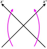
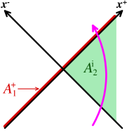
Figure 1: Left : decomposition of the solution of the Dirac equation into left-moving and right-moving partial waves. Right : structure of the gauge field produced by the two nuclei in the $A^{-}=0$ gauge, that we use for solving the Dirac equation for the right-moving partial wave. $x^{\pm}$ denote light-cone coordinates, $x^{\pm}\equiv(t\pm z)/\sqrt{2}$.

For the right-moving partial wave, it is convenient to work in the light-cone gauge $A^{-}=0$, in the same spirit as what was done in ref. [45] for the gluons. After having determined the right-moving spinor at the proper time $\tau_{0}$ inside the forward light-cone, we will rotate it to the Fock-Schwinger gauge. The calculation for the left-moving spinor (to be performed in the light-cone gauge $A^{+}=0$) will not be performed here, since the result can be guessed from the other partial wave by symmetry. The structure of the background field in the $A^{-}=0$ is shown in the right diagram of the figure 1. It is made of the following two elements :

• the nucleus moving in the $+z$ direction produces a field $A_{1}^{+}$, proportional to a $\delta(x^{-})$ and independent of $x^{+}$.

• in the region $x^{+}>0,x^{-}<0$, the nucleus moving in the $-z$ direction produces a field $A_{1}^{i}$, which has the form of a transverse pure gauge,

  $$A_{2}^{i}=\frac{i}{g}\,U_{2}^{\dagger}\partial^{i}U_{2}\;.$$ (47)

• in the strip corresponding to the shock-wave of the nucleus moving in the $+z$ direction, this field $A_{2}^{i}$ receives a color precession induced by the first nucleus. This color rotated field reads

  $$\alpha_{2}^{ia}=\frac{i}{g}U_{1ab}(x^{-},{\bm{x}}_{\perp})\,(U_{2}^{\dagger}\partial^{i}U_{2})_{b}\;,$$ (48)

  where

  $$U_{1}(x^{-},{\bm{x}}_{\perp})={\rm T}\;\exp ig\int_{0}^{x^{-}}dz^{-}\;A_{1}^{+}(z^{-},{\bm{x}}_{\perp})\;.$$ (49)

  Note that eq. (48) is equivalent to

  $$\alpha_{2}^{i}\equiv\alpha_{2}^{ia}t^{a}=U_{1}A_{2}^{i}U_{1}^{\dagger}\;.$$ (50)

Therefore, by starting the evolution at $x^{0}=-\infty$, the right-moving partial wave encounters first the field $A_{2}^{i}$ and then the field $A_{1}^{+}$. In order to express the quark spectrum, we need the negative energy spinors, $\psi^{-}_{{\bm{k}}sa}$ (${\bm{k}}$ is the 3-momentum of the incoming quark, $s$ its spin and $a$ its color). Before they encounter the background color field, they read simply

$$\psi^{-}_{{\bm{k}}sa}(x)=v_{s}({\bm{k}})\,e^{+ik\cdot x}\;.$$ (51)

Since the background color field has only a finite jump on the half-line $x^{+}=0,x^{-}<0$, the spinors are continuous across this line, and the above formulas remain valid up to $x^{+}=0^{+}$ (just above this line).

4.2 Evolution in the region $x^{-}<0,x^{+}>0$

The next step is to solve the Dirac equation in the region $x^{+}>0,x^{-}<0$. Since the background field is a pure gauge in this region, the covariant derivative can be written as

$$D^{\mu}=U_{2}^{\dagger}\,\partial^{\mu}\,U_{2}\;.$$ (52)

Therefore, the new spinor defined by $\breve{\psi}_{{\bm{k}}sa}^{-}\equiv U_{2}\,\psi_{{\bm{k}}sa}^{-}$ obeys the free Dirac equation :

$$(i\raise 0.6458pt\hbox{$/$}\kern-5.29999pt\hbox{$\partial$}-m)\breve{\psi}_{{\bm{k}}sa}^{-}=0\;.$$ (53)

The solution of this equation can be expressed in terms of the initial value of $\breve{\psi}_{{\bm{k}}sa}^{-}$ on the surface $x^{+}=0^{+}$ by the following Green’s formula,

$$\breve{\psi}_{{\bm{k}}sa}^{-}(x)=i\int_{y^{+}=0}dy^{-}d^{2}{\bm{y}}_{\perp}\;S_{{}_{R}}^{0}(x,y)\,\gamma^{+}\,\breve{\psi}_{{\bm{k}}sa}^{-}(y)\;,$$ (54)

where $S_{{}_{R}}^{0}(x,y)$ is the bare retarded propagator for a quark,

$$S_{{}_{R}}^{0}(x,y)\equiv\int\frac{d^{4}{\bm{p}}}{(2\pi)^{4}}\;\frac{e^{-ip\cdot(x-y)}}{\raise 0.43057pt\hbox{$/$}\kern-6.30005pt\hbox{$p$}-m+ip_{0}\gamma^{0}\epsilon}\;.$$ (55)

Note that, even if we have not restricted the integration range for the variable $y^{-}$ in eq. (54), the fact that the support of the retarded propagator $S_{{}_{R}}^{0}$ is limited to $x^{0}>y^{0},(x-y)^{2}\geq 0$ imposes that $y^{-}\leq x^{-}$. Therefore, for a point $x$ located in the region $x^{+}>0,x^{-}<0$ (shaded in green in the figure 1), only points with $y^{-}<0$ on the initial surface can contribute. This is the reason we can solve independently the equation for the left- and right-moving partial waves.

By introducing the Fourier representation (55) of the retarded propagator in the Green’s formula (54), one can perform most of the integrations analytically except the final integration over transverse momentum. This leads to

$${\psi}^{-}_{{\bm{k}}sa}(x) = U_{2}^{\dagger}({\bm{x}}_{\perp})\smash{\int\frac{d^{2}{\bm{p}}_{\perp}}{(2\pi)^{2}}}\;e^{i{\bm{p}}_{\perp}\cdot{\bm{x}}_{\perp}}\,e^{i(k^{+}x^{-}+\frac{M_{\bm{p}}^{2}}{2k^{+}}x^{+})}\,\widetilde{U}_{2}({\bm{p}}_{\perp}+{\bm{k}}_{\perp})$$ (56)

$$\qquad\qquad\qquad\qquad\times\left(1-\gamma^{+}\frac{p^{i}\gamma^{i}+m}{2k^{+}}\right){\cal P}^{+}v_{s}({\bm{k}})\;,$$

where $M_{\bm{p}}\equiv\sqrt{{\bm{p}}_{\perp}^{2}+m^{2}}$ is the transverse mass and where we have introduced the projector ${\cal P}^{+}\equiv\gamma^{-}\gamma^{+}/2$. We have also introduced the Fourier transform of the Wilson line $U_{2}$

$$\widetilde{U}_{2}({\bm{k}}_{\perp})\equiv\int d^{2}{\bm{y}}_{\perp}\;e^{-i{\bm{k}}_{\perp}\cdot{\bm{y}}_{\perp}}\;U_{2}({\bm{y}}_{\perp})\;.$$ (57)

One can check that eq. (56) falls back to the free spinor $v_{s}({\bm{k}})\exp(ik\cdot x)$ if the background field is turned off ($U_{2}=1$).

4.3 Evolution across the line $x^{-}=0~{}~{}~{}(x^{+}>0)$

The next step is to propagate the spinor (56) across the field $A_{1}^{+}$ of the nucleus moving in the $+z$ direction. The region of space-time supporting this field is infinitesimal (since $A_{1}^{+}\sim\delta(x^{-})$), but the infinite strength of the gauge field in this region nevertheless produces a finite change of the spinors. In this region, there is also an ${\cal O}(1)$ transverse component of the gauge field, given in eq. (48). The Dirac equation,

$$\left[i(\partial^{+}-igA_{1}^{+})\gamma^{-}+i\partial^{-}\gamma^{+}-iD^{i}\gamma^{i}-m\right]\,\psi^{-}=0\;,$$ (58)

can be separated into a part that depends on the background field $A_{1}^{+}$ and a constraint independent of $A_{1}^{+}$ by multiplying it by the projectors ${\cal P}^{+}$ or ${\cal P}^{-}\equiv\gamma^{+}\gamma^{-}/2$ :

$$i\partial^{-}{\cal P}^{+}\psi_{{\bm{k}}sa}^{-} = \frac{m-i\gamma^{i}D^{i}}{2}\gamma^{-}{\cal P}^{-}\psi_{{\bm{k}}sa}^{-}$$

$$i(\partial^{+}-igA_{1}^{+}){\cal P}^{-}\psi_{{\bm{k}}sa}^{-} = \frac{\gamma^{+}(i\gamma^{i}D^{i}+m)}{2}\psi_{{\bm{k}}sa}^{-}\;.$$ (59)

The first equation, independent of the background field, is a constraint that relates the two projections of the spinors at every $x^{-}$ (note that this equation does not contain the $\partial^{+}$ derivative). The second equation determines the dynamical evolution (in the variable $x^{-}$) of the ${\cal P}^{-}$ projection under the influence of the background field $A_{1}^{+}$. Inserting the first equation into the second gives a second order equation that drives the evolution of the ${\cal P}^{-}$ projection,

$$\left(2\partial^{-}(\partial^{+}-igA_{1}^{+})-D_{\perp}^{2}+m^{2}\right)\,{\cal P}^{-}\psi_{{\bm{k}}sa}^{-}=0\;.$$ (60)

In this equation, the $\partial^{+}$ derivative and the field $A_{1}^{+}$ are large (inversely proportional to the thickness of the shock-wave that supports the $A_{1}^{+}$ field), while all the other terms do not have this large factor. Physically, keeping only the term in $\partial^{+}-igA_{1}^{+}$ leads to the eikonal approximation, where the fermion would propagate on a straight line along the $x^{-}$ axis, while the terms $-D_{\perp}^{2}+m^{2}$ lead to some transverse diffusion with respect to this axis. In the limit where the thickness of the shock-wave goes to zero, we can neglect it :

$$i(\partial^{+}-igA_{1}^{+}){\cal P}^{-}\psi_{{\bm{k}}sa}^{-}=0\;.$$ (61)

(Note that this approximation is only valid to cross the shock-wave, and should not be used to evolve at a finite distance from the shock-wave.) The solution of this equation is very simple,

$${\cal P}^{-}\psi_{{\bm{k}}sa}^{-}(x)=U_{1}(x^{-},{\bm{x}}_{\perp})\,{\cal P}^{-}\psi_{{\bm{k}}sa}^{-}(0,x^{+},{\bm{x}}_{\perp})\;,$$ (62)

where the $x^{-}$-dependent Wilson line $U_{1}$ was defined in eq. (49). The spinor at $x^{-}=0$ that appears in the right hand side is given by eq. (56). Then, the constraint equation can be solved to give

$${\cal P}^{+}\psi_{{\bm{k}}sa}^{-}(x)=-i\int^{x^{+}}dz^{+}\;\frac{m-i\gamma^{i}D^{i}}{2}\gamma^{-}\,U_{1}(x^{-},{\bm{x}}_{\perp})\,{\cal P}^{-}\psi_{{\bm{k}}sa}^{-}(0,z^{+},{\bm{x}}_{\perp})\;.$$ (63)

Note that the constraint defines the ${\cal P}^{+}$ projection of the spinor only up to an arbitrary function of $x^{-}$ and ${\bm{x}}_{\perp}$. This “integration constant” can be determined by requesting that we recover the ${\cal P}^{+}$ projection of a free spinor when all the Wilson lines are set to the identity.

4.4 Transformation to Fock-Schwinger gauge

In order to gauge transform these spinors to the Fock-Schwinger gauge, it is sufficient to multiply them by $U_{1}^{\dagger}$,

$$\psi_{{\bm{k}}sa\,{}_{\rm FS}}^{-}(x)=U_{1}^{\dagger}({\bm{x}}_{\perp})\,\psi_{{\bm{k}}sa}^{-}(x)\;.$$ (64)

When this transformation is applied to eqs. (62) and (63), the Wilson line $U_{1}$ appears in two types of combinations :

$$U_{1}^{\dagger}U_{1}=1\qquad\mbox{and}\qquad U_{1}^{\dagger}D^{i}U_{1}\;.$$ (65)

The second of these structures can be simplified if we recall that $D^{i}$ is the covariant derivative built with the field of eq. (50). Therefore,

$$U_{1}^{\dagger}D^{i}U_{1} = U_{1}^{\dagger}(\partial^{i}-igU_{1}A_{2}^{i}U_{1}^{\dagger})U_{1}$$ (66)

$$= \underbrace{\partial^{i}-ig(A_{1}^{i}+A_{2}^{i})}_{D^{i}_{{}_{\rm FS}}}\;,$$

where $A_{1}^{i}$ is defined in the same way as $A_{2}^{i}$ (see the eq. (47)),

$$A_{1}^{i}\equiv\frac{i}{g}\,U_{1}^{\dagger}\partial^{i}U_{1}\;.$$ (67)

Note that the field $A_{1}^{i}+A_{2}^{i}$ that appears in this equation is nothing but the transverse component of the gauge potential in the Fock-Schwinger gauge at $\tau=0^{+}$, hence the notation $D_{{}_{\rm FS}}^{i}$ for the resulting covariant derivative. Therefore, the two projections of the right-moving negative energy spinors in the Fock-Schwinger gauge read (at $x^{-}=0^{+}$, just above the shock-wave)

$${\cal P}^{-}\psi_{{\bm{k}}sa\,{}_{\rm FS}}^{-}(x) = U_{2}^{\dagger}({\bm{x}}_{\perp})\smash{\int\frac{d^{2}{\bm{p}}_{\perp}}{(2\pi)^{2}}}\;e^{i{\bm{p}}_{\perp}\cdot{\bm{x}}_{\perp}}\,e^{i\frac{M_{\bm{p}}^{2}}{2k^{+}}x^{+}}$$

$$\qquad\qquad\times\;\widetilde{U}_{2}({\bm{p}}_{\perp}+{\bm{k}}_{\perp})\,\frac{p^{i}\gamma^{i}-m}{2k^{+}}\,\gamma^{+}\,v_{s}({\bm{k}})$$

$${\cal P}^{+}\psi_{{\bm{k}}sa\,{}_{\rm FS}}^{-}(x) = (i\gamma^{i}D^{i}_{{}_{\rm FS}}-m)\,U_{2}^{\dagger}({\bm{x}}_{\perp})\smash{\int\frac{d^{2}{\bm{p}}_{\perp}}{(2\pi)^{2}}}\;e^{i{\bm{p}}_{\perp}\cdot{\bm{x}}_{\perp}}\,e^{i\frac{M_{\bm{p}}^{2}}{2k^{+}}x^{+}}$$ (68)

$$\qquad\qquad\times\;\widetilde{U}_{2}({\bm{p}}_{\perp}+{\bm{k}}_{\perp})\,\gamma^{-}\,\frac{p^{i}\gamma^{i}-m}{2M_{\bm{p}}^{2}}\,\gamma^{+}\,v_{s}({\bm{k}})$$

The eqs. (68) for the right-moving spinors must be completed by a set of similar equations for the left-moving spinors. These can be obtained from the above formulas by the following substitutions

$$U_{2} \to U_{1}$$

$$x^{+} \to x^{-}\quad,\quad k^{+}\;\to\;k^{-}$$

$${\cal P}^{+} \to {\cal P}^{-}\quad,\quad{\cal P}^{-}\;\to\;{\cal P}^{+}$$

$$\gamma^{+} \to \gamma^{-}\quad,\quad\gamma^{-}\;\to\;\gamma^{+}\;.$$ (69)

At this point, we have the components of the negative energy mode functions on the light-cone $\tau=0^{+}$ (i.e. just after the collision), which provides all the necessary initial data for studying their evolution after the collision. As explained in the appendix C, these formulas can also be used as initial conditions at some initial time $\tau_{0}>0$, provided that $\tau_{0}\ll a_{\perp}$ where $a_{\perp}$ is the transverse lattice spacing used in the numerical resolution.

4.5 Mode functions in the $\nu$ basis

So far, we have derived the mode functions $\psi_{{\bm{k}}sa}$ in terms of the Cartesian 3-momentum ${\bm{k}}$. However, as explained in the section 2.3,the boost invariance of a high energy collision is more manifest if one uses the modified spinors defined in eq. (13) and if one further goes to a basis where the spinors are labeled by the quantum number $\nu$ (Fourier conjugate to $\eta$) instead of $y$. It is easy to obtain these new mode functions by the following transformation :

$$\widehat{\psi}{}_{{\bm{k}}_{\perp}\nu sa}\equiv\sqrt{\tau}\;e^{-\frac{\eta}{2}\gamma^{0}\gamma^{3}}\int_{-\infty}^{+\infty}dy\;e^{i\nu y}\;\psi{}_{{\bm{k}}_{\perp}ysa}\;.$$ (70)

For the right-moving partial waves, the integral that enters in the transformation of ${\cal P}^{\epsilon}\psi^{-}$ is of the form

$$I^{\epsilon}_{{}_{\rm R}}\equiv\int_{-\infty}^{+\infty}dy\;e^{i\nu y}\;e^{\epsilon\frac{y}{2}}\;e^{i\alpha e^{-y}}\;,$$ (71)

while for the left moving partial waves, one needs

$$I^{\epsilon}_{{}_{\rm L}}\equiv\int_{-\infty}^{+\infty}dy\;e^{i\nu y}\;e^{\epsilon\frac{y}{2}}\;e^{i\alpha e^{+y}}\;.$$ (72)

These integrals can be expressed in terms of the $\Gamma$ function,

$$I_{{}_{\rm R}}^{\epsilon}=(-i\alpha)^{i\nu+\frac{\epsilon}{2}}\,\Gamma\big{(}-i\nu-\tfrac{\epsilon}{2}\big{)}\quad,\quad I_{{}_{\rm L}}^{\epsilon}=(-i\alpha)^{-i\nu-\frac{\epsilon}{2}}\,\Gamma\big{(}i\nu+\tfrac{\epsilon}{2}\big{)}\;.$$ (73)

Let us now recapitulate our results for the fermionic mode functions on the light-cone after this transformation, after summing the right-moving and left-moving partial waves, and including both the ${\cal P}^{+}$ and ${\cal P}^{-}$ projections

$$\widehat{\psi}_{{\bm{k}}_{\perp}\nu sa\,{}_{\rm FS}}^{-}(x)\mathrel{\mathop{\kern 0.0pt=}\limits_{\tau\to 0^{+}}}-\frac{e^{i\frac{\pi}{4}}}{\sqrt{M_{\bm{k}}}}\;e^{i\nu\eta}{\int\frac{d^{2}{\bm{p}}_{\perp}}{(2\pi)^{2}}}\;{\frac{e^{i{\bm{p}}_{\perp}\cdot{\bm{x}}_{\perp}}}{M_{\bm{p}}}}\;$$

$$\!\!\!\!\times\Bigg{\{}e^{\frac{\pi\nu}{2}}\Big{(}\tfrac{M_{\bm{p}}^{2}\tau}{2M_{\bm{k}}}\Big{)}^{i\nu}\!\Gamma(-i\nu\!+\!{\tfrac{1}{2}})U_{2}^{\dagger}({\bm{x}}_{\perp})\widetilde{U}_{2}({\bm{p}}_{\perp}\!+\!{\bm{k}}_{\perp})\gamma^{+}$$

$$\!\!\!\!+e^{-\frac{\pi\nu}{2}}\Big{(}\tfrac{M_{\bm{p}}^{2}\tau}{2M_{\bm{k}}}\Big{)}^{-i\nu}\!\Gamma(i\nu\!+\!{\tfrac{1}{2}})U_{1}^{\dagger}({\bm{x}}_{\perp})\widetilde{U}_{1}({\bm{p}}_{\perp}\!+\!{\bm{k}}_{\perp})\gamma^{-}\!\Bigg{\}}(p^{i}\gamma^{i}\!+\!m)v_{s}({\bm{k}}_{\perp},y\!=\!0)\,.$$

(74)

In this formula, we have kept only the terms that are non-vanishing in the limit $\tau\to 0^{+}$. Therefore, its use should be restricted to very early times.

5 Summary and outlook

In this paper, we have reconsidered the problem of quark production in heavy ion collisions in the color glass condensate framework. Our approach is closely following that of refs. [31, 32], which expresses the leading order inclusive quark spectrum in terms of a set of mode functions of the Dirac equation, but overcomes a number of limitations of this earlier work.

Firstly, we have defined a basis of fermionic mode functions that are more appropriate for the boost invariant expanding geometry of a high energy collision. In particular, since these mode functions are indexed by the Fourier conjugate $\nu$ to rapidity, they are especially suitable for a lattice implementation in which one discretizes the rapidity axis. We have calculated analytically the value of these mode functions just after the collision, at a proper time $Q_{s}\tau\ll 1$ and in the Fock-Schwinger gauge, in terms of the Wilson lines that represent the classical color background field of the two colliding nuclei. Thanks to these analytical initial values, one will not have to deal with crossing the light-cones in the numerical resolution of the Dirac equation.

Secondly, we have exposed a statistical method for sampling the set of modes over which one must sum in the calculation of the quark spectrum. This method ensures that no mode is left out, while considerably reducing the computing time compared to a complete sum over all the modes. This approach also provides a more robust way of estimating the error one makes in the sum over the modes functions.

In a forthcoming paper, we will apply the formalism that we have setup in the present paper to a study of quark production in two situations. Firstly, we will present a test of the method in the case of a background field for which one can solve analytically the Dirac equation for the mode functions (a constant $SU(2)$ chromo-electrical field). Then, we will present results on quark production in heavy ion collisions, in the case where the background color field is given by the MV model. In order to mitigate the problems caused by the lattice fermion doubler modes, we will also explain how our framework must be modified in order to include a Wilson term in the fermionic action.

Appendix A Quark spectrum in the Schwinger-Keldysh formalism

In this appendix, we recall the derivation of the formulas (4) for the inclusive quark spectrum, starting from the standard LSZ reduction formulas. For simplicity, we consider only one flavor of quarks. Since in the CGC framework, the external sources are only coupled to gluons and quarks can only produced in quark-antiquark pairs (the net flavor number is always zero).

A.1 Single quark pair amplitude

Firstly, let us consider the amplitude for producing a single quark-antiquark pair,

$${\cal M}_{1}({\bm{p}},{\bm{q}}) \equiv \big{<}Q({\bm{p}}),\overline{Q}({\bm{q}}){}_{\rm out}\big{|}0{}_{\rm in}\big{>}$$ (75)

$$= \big{<}0{}_{\rm out}\big{|}b_{\rm out}({\bm{p}})d_{\rm out}({\bm{q}})\big{|}0{}_{\rm in}\big{>}\;.$$

In order to keep the notations concise, we are not writing explicitly the color and spin indices of the quark and antiquark. The operator $b_{\rm out}^{\dagger}({\bm{p}})$ (resp. $d_{\rm out}^{\dagger}({\bm{q}})$) creates a quark of momentum ${\bm{p}}$ (resp. an antiquark of momentum ${\bm{q}}$).

Using the decomposition of the free field operator $\psi_{\rm out}(x)$ as a superposition of free modes, we have

$$b_{\rm out}({\bm{p}}) = \int d^{3}{\bm{x}}\;\overline{u}({\bm{p}})\gamma^{0}\;\psi_{\rm out}(t,{\bm{x}})\;e^{ip\cdot x}$$

$$d_{\rm out}({\bm{q}}) = \int d^{3}{\bm{x}}\;\overline{\psi}_{\rm out}(t,{\bm{x}})\gamma^{0}\;v({\bm{q}})\;e^{iq\cdot x}\;.$$ (76)

(In these formulas, $p^{0}=\sqrt{{\bm{p}}^{2}+m^{2}}$ and $q^{0}=\sqrt{{\bm{q}}^{2}+m^{2}}$.) Note that the time $t$ at which these formulas are evaluated do not change the result. Using these formulas, standard manipulations lead to the LSZ reduction formulas for the single quark pair production amplitude,

$${\cal M}_{1}({\bm{p}},{\bm{q}}) = \int d^{4}x\,d^{4}y\;e^{ip\cdot x}\,\overline{u}({\bm{p}})(i\stackrel{{\scriptstyle\rightarrow}}{{\raise 0.6458pt\hbox{$/$}\kern-5.29999pt\hbox{$\partial$}}}_{x}-m)$$ (77)

$$\times\big{<}0{}_{\rm out}\big{|}{\rm T}\psi(x)\overline{\psi}(y)\big{|}0{}_{\rm in}\big{>}\;(i\stackrel{{\scriptstyle\leftarrow}}{{\raise 0.6458pt\hbox{$/$}\kern-5.29999pt\hbox{$\partial$}}}_{y}+m)\;v({\bm{q}})\,e^{iq\cdot y}\;.$$

Note that the 2-point correlation function that appears in this formula is a Feynman (i.e. time-ordered) propagator. Its evaluation to all orders in the background gluon field cannot be performed in practice. Indeed, even though it obeys the Dirac equation, its determination is made extremely complicated by the fact that it must satisfy mixed boundary conditions, both at $x^{0}=-\infty$ and at $x^{0}=+\infty$.

A.2 Inclusive quark spectrum

There is no practical way to calculate the single quark amplitude considered in the previous subsection, in the presence of a strong background gluon field, as is the case in the high energy heavy ion collisions. This is not a big limitation however, because this quantity is also not very phenomenologically useful in such a context. Indeed, for light quarks (quark flavors for which $m\lesssim Q_{s}$), quark production is not a rare process and more than one quark pair are produced in a collision. Therefore, the probability $P_{1}$ of producing exactly one quark pair (given by the square of ${\cal M}_{1}$) is not very interesting.

Much more useful would be the complete probability distribution, $P_{1}$, $P_{2}$, $P_{3}$, etc. Unfortunately, calculating them is as complicated as calculating $P_{1}$. But it turns out that the moments of the probability distribution are much easier to compute. Besides the trivial one ($\sum_{n=0}^{\infty}P_{n}=1$), the simplest of these moments is the first moment, $\sum_{n}nP_{n}$, that gives the mean number of produced pairs. A little more information can be gathered by considering the same quantity in differential form, which is precisely the quark spectrum. In terms of transition amplitudes, this quantity reads

$$\frac{dN_{\rm q}}{d^{3}{\bm{p}}} \equiv \frac{1}{(2\pi)^{3}2\omega_{\bm{p}}}\,\sum_{n=0}^{+\infty}(n+1)\frac{1}{(n+1)!^{2}}\int d\Phi_{\bm{q}}\prod_{i=1}^{n}d\Phi_{{\bm{p}}_{i}}d\Phi_{{\bm{q}}_{i}}$$

$$\!\!\!\times\left|\big{<}0{}_{\rm out}\big{|}b_{\rm out}({\bm{p}})d_{\rm out}({\bm{q}})b_{\rm out}({\bm{p}}_{1})d_{\rm out}({\bm{q}}_{1})\cdots b_{\rm out}({\bm{p}}_{n})d_{\rm out}({\bm{q}}_{n})\big{|}0{}_{\rm in}\big{>}\right|^{2}\;.$$

where we have used the shorthand

$$d\Phi_{\bm{q}}\equiv\frac{d^{3}{\bm{q}}}{(2\pi)^{3}2\omega_{\bm{q}}}$$ (79)

for the invariant phase-space of final state quarks and antiquarks. In this formula, the differential probability for producing $n+1$ quark-antiquark pairs is weighted by the number of quarks ($n+1$), and then integrated over the phase-space of all the antiquarks and of $n$ of the quarks. This quantity is normalized in such a way that it gives the mean number of produced quarks after integration over $d^{3}{\bm{p}}$,

$$\int d^{3}{\bm{p}}\;\frac{dN_{\rm q}}{d^{3}{\bm{p}}}=\sum_{n=0}^{+\infty}nP_{n}\equiv\left<N_{\rm q}\right>\;.$$ (80)

Most of eq. (LABEL:eq:spectrum-def) is in fact the projector on the subspace of states with net flavor number $-1$,

$${\bm{1}} \equiv \sum_{n=0}^{+\infty}\frac{1}{n!(n+1)!}\int d\Phi_{\bm{q}}\prod_{i=1}^{n}d\Phi_{{\bm{p}}_{i}}d\Phi_{{\bm{q}}_{i}}$$ (81)

$$\!\!\!\!\times\big{|}[{\bm{p}}_{1}\cdots{\bm{p}}_{n}]_{{}_{Q}}[{\bm{q}}{\bm{q}}_{1}\cdots{\bm{q}}_{n}]_{{}_{\overline{Q}}}\;{}_{\rm out}\big{>}\big{<}[{\bm{p}}_{1}\cdots{\bm{p}}_{n}]_{{}_{Q}}[{\bm{q}}{\bm{q}}_{1}\cdots{\bm{q}}_{n}]_{{}_{\overline{Q}}}\;{}_{\rm out}\big{|}\;,$$

that has a trivial action on the state $b_{\rm out}({\bm{p}})\big{|}0{}_{\rm in}\big{>}$ (since this state has also flavor number $-1$), and eq. (LABEL:eq:spectrum-def) can then be reduced to the much more compact form

$$\frac{dN_{\rm q}}{d^{3}{\bm{p}}}=\frac{1}{(2\pi)^{3}2\omega_{\bm{p}}}\;\big{<}0{}_{\rm in}\big{|}b_{\rm out}^{\dagger}({\bm{p}})b_{\rm out}({\bm{p}})\big{|}0{}_{\rm in}\big{>}\;.$$ (82)

The interpretation of this formula is quite transparent, since it amounts to evaluating the expectation value of the final quark number operator, for a system prepared in the pure state $\big{|}0{}_{\rm in}\big{>}$.

Using eqs. (76), this can be rewritten in terms of the quark field operator as follows,

$$\frac{dN_{\rm q}}{d^{3}{\bm{p}}} = \frac{1}{(2\pi)^{3}2\omega_{\bm{p}}}\;\int d^{4}x\,d^{4}y\;e^{ip\cdot x}\;\overline{u}({\bm{p}})\,(i\stackrel{{\scriptstyle\rightarrow}}{{\raise 0.6458pt\hbox{$/$}\kern-5.29999pt\hbox{$\partial$}}}_{x}-m)$$ (83)

$$\times\big{<}0{}_{\rm in}\big{|}\psi(x)\overline{\psi}(y)\big{|}0{}_{\rm in}\big{>}\;(i\stackrel{{\scriptstyle\leftarrow}}{{\raise 0.6458pt\hbox{$/$}\kern-5.29999pt\hbox{$\partial$}}}_{y}-m)\;e^{-ip\cdot y}\,u({\bm{p}})\;.$$

The main differences between this expression and the similar expression for the amplitude ${\cal M}_{1}$ are the following :

• The vacuum state is the in-vacuum state on both sides.

• The two spinors are not time ordered.

These differences in fact lead to considerable simplifications in the evaluation of this quantity in the presence of a strong background gluon field.

The first step is to note that the 2-point correlator that appears in the integrand of eq. (83) is the component $S_{-+}(x,y)$ of the fermion 2-point function in the Schwinger-Keldysh formalism. In the presence of a background field $A^{\mu}$, its tree level expression (to all orders in the background field) can be obtained by noticing that it obeys the following equations

$$(i\stackrel{{\scriptstyle\longrightarrow}}{{\raise 0.6458pt\hbox{$/$}\kern-6.69998pt\hbox{$D$}}}_{x}-m)\,{\cal S}_{-+}(x,y)=0\;,\quad{\cal S}_{-+}(x,y)\,(i\stackrel{{\scriptstyle\longleftarrow}}{{\raise 0.6458pt\hbox{$/$}\kern-6.69998pt\hbox{$D$}}}_{y}-m)=0$$

$$\lim_{x^{0},y^{0}\to-\infty}{\cal S}_{-+}(x,y)={\cal S}_{-+}^{\rm vacuum}(x,y)\;.$$ (84)

Next, one should recall the expression of the vacuum propagator ${\cal S}_{-+}^{\rm vacuum}(x,y)$,

$${\cal S}_{-+}^{\rm vacuum}(x,y)=\sum_{\genfrac{}{}{0.0pt}{}{s=\uparrow,\downarrow}{a}}\int\frac{d^{3}{\bm{k}}}{(2\pi)^{3}2\omega_{\bm{k}}}\;e^{ik\cdot(x-y)}\;v_{s}({\bm{k}})\overline{v}_{s}({\bm{k}})\;.$$ (85)

It is then easy to construct a semi-explicit expression for the dressed propagator ${\cal S}_{-+}(x,y)$ in terms of a basis of solutions of the Dirac equation:

$$S_{-+}(x,y)=\sum_{\genfrac{}{}{0.0pt}{}{s=\uparrow,\downarrow}{a}}\int\frac{d^{3}{\bm{k}}}{(2\pi)^{3}2\omega_{\bm{k}}}\;\psi_{{\bm{k}}sa}(x)\overline{\psi}_{{\bm{k}}sa}(y)$$

$$(i\raise 0.6458pt\hbox{$/$}\kern-6.69998pt\hbox{$D$}_{x}-m)\,\psi_{{\bm{k}}sa}(x)=0\quad,\quad\lim_{x^{0}\to-\infty}\psi_{{\bm{k}}sa}(x)=v_{s}({\bm{k}})\,e^{ik\cdot x}\;.$$ (86)

When this expression is inserted into eq. (83), one must evaluate the following expression

$$\int d^{4}x\;e^{ip\cdot x}\;\overline{u}_{\sigma}({\bm{p}})\,(i\stackrel{{\scriptstyle\rightarrow}}{{\raise 0.6458pt\hbox{$/$}\kern-5.29999pt\hbox{$\partial$}}}_{x}-m)\;\psi_{{\bm{k}}sa}(x)\;.$$ (87)

It is useful to note that

$$e^{ip\cdot x}\;\overline{u}_{\sigma}({\bm{p}})\,(i\stackrel{{\scriptstyle\leftarrow}}{{\raise 0.6458pt\hbox{$/$}\kern-5.29999pt\hbox{$\partial$}}}_{x}+m)=0\;.$$ (88)

Adding this identity to the integrand of eq. (87), we obtain

$$\int d^{4}x\,e^{ip\cdot x}\,\overline{u}_{\sigma}({\bm{p}})\,(i\stackrel{{\scriptstyle\rightarrow}}{{\raise 0.6458pt\hbox{$/$}\kern-5.29999pt\hbox{$\partial$}}}_{x}\!-\!m)\,\psi_{{\bm{k}}sa}(x)=i\int d^{4}x\,\partial_{\mu}\left[e^{ip\cdot x}\,\overline{u}_{\sigma}({\bm{p}})\gamma^{\mu}\,\psi_{{\bm{k}}sa}(x)\right]\,,$$ (89)

which can be rewritten as a 3-dimensional integral since it is the integral of a total derivative. The boundary at spatial infinity can be dropped if there are no background fields there. The boundary at $x^{0}\to-\infty$ does not contribute because it leads to the vanishing overlap $u^{\dagger}({\bm{p}})v({\bm{p}})$. The only remaining contribution comes from $x^{0}\to\infty$,

$$\int d^{4}x\;e^{ip\cdot x}\;\overline{u}_{\sigma}({\bm{p}})\,(i\stackrel{{\scriptstyle\rightarrow}}{{\raise 0.6458pt\hbox{$/$}\kern-5.29999pt\hbox{$\partial$}}}_{x}-m)\;\psi_{{\bm{k}}sa}(x)=i\lim_{x^{0}\to+\infty}\int d^{3}{\bm{x}}\;e^{ip\cdot x}\;{u}^{\dagger}_{\sigma}({\bm{p}})\;\psi_{{\bm{k}}sa}(x)\;.$$ (90)

This formula leads immediately to eq. (4).

Appendix B Quark spectrum from Feynman amplitudes

In the previous appendix, we presented a derivation of the quark spectrum based on fairly standard many-body manipulations: we first related this spectrum to the expectation value of the quark number operator, and then we evaluated the latter using the Schwinger-Keldysh formalism. However, a more elementary derivation is possible, where the many-body aspects of the problem are treated “by hand”. In the present appendix, we present such an alternate derivation, starting from the Feynman amplitudes for producing 1,2,3,… quark-antiquark pairs, and combining them in the appropriate way to obtain the single quark spectrum. This method is a bit more involved since it requires to account for all the final state particle permutations, but it has the advantage of making more tangible the combinatorics that happens under the hood in the derivation of the appendix A.

B.1 Pair production amplitudes

The starting point is the amplitude ${\cal M}_{1}({\bm{p}},{\bm{q}})$ for producing one quark-antiquark pair, already introduced in eq. (75). This amplitude is made of a time ordered 2-point function connecting the quark of momentum ${\bm{p}}$ and the antiquark of momentum ${\bm{q}}$, times a disconnected sum of vacuum-vacuum graphs. The latter is crucial in the presence of a background field, since the sum of the vacuum-vacuum graphs is not a pure phase (unlike when the background is the vacuum). In practice, we do not need to calculate this factor, since it is the same in all amplitudes and can therefore be determined at the very end by the request that the sum of all probabilities to produce 0,1,2,3,… quarks is equal to one. For now, we will simply write

$${\cal M}_{1}({\bm{p}},{\bm{q}})\equiv\underbrace{\big{<}0{}_{\rm out}\big{|}0{}_{\rm in}\big{>}}_{\mbox{\scriptsize sum of vacuum graphs}}\times\;{\cal M}_{1}^{c}({\bm{p}},{\bm{q}})\;,$$ (91)

where ${\cal M}_{1}^{c}$ is the connected part of the pair production amplitude (only this factor carries a dependence on the momenta of the produced quark and antiquark).

In the rest of this appendix, we limit the discussion to the lowest order for the factor ${\cal M}_{1}^{c}$. At this order, it is simply made of a Feynman propagator connecting the produced quark and antiquark, dressed by the background field:

$${\cal M}_{1}^{c}({\bm{p}},{\bm{q}})=\raise-34.1433pt\hbox to56.9055pt{\leavevmode\resizebox{56.9055pt}{}{\includegraphics{M1c}}}$$ (92)

For the sake of simplicity, we will represent this dressed propagator as follows:

$$\raise-34.1433pt\hbox to56.9055pt{\leavevmode\resizebox{56.9055pt}{}{\includegraphics{M1c}}}\quad=\quad\raise-34.1433pt\hbox to39.83368pt{\leavevmode\resizebox{39.83368pt}{}{\includegraphics{M1c1}}}\quad\;.$$ (93)

A more explicit expression of the connected part of the single pair production amplitude is

$${\cal M}_{1}^{c}({\bm{p}},{\bm{q}})=\overline{u}({\bm{p}})T_{{}_{F}}(p,-q)v({\bm{q}})\;,$$ (94)

where $T_{{}_{F}}$ is the dressed Feynman propagator, amputated of its final free propagators. In terms of the dressed ($G_{{}_{F}}$) and free ($G_{{}_{F}}^{0}$) Feynman propagators, it is given by

$$G_{{}_{F}}=G_{{}_{F}}^{0}+G_{{}_{F}}^{0}\;T_{{}_{F}}\;G_{{}_{F}}^{0}\;.$$ (95)

The convention for the momenta in eq. (94) is that the 4-momentum $-q$ enters on one side of the propagator and the 4-momentum $p$ exits on the other side.

At the same level of approximation, the amplitude for producing $n$ pairs is obtained as follows:

$${\cal M}_{n}({\bm{p}}_{1}\cdots{\bm{p}}_{n},{\bm{q}}_{1}\cdots{\bm{q}}_{n})={\big{<}0{}_{\rm out}\big{|}0{}_{\rm in}\big{>}}\sum_{\sigma\in{\mathfrak{S}}_{n}}\epsilon(\sigma)\;{\cal M}_{1}^{c}({\bm{p}}_{1},{\bm{q}}_{\sigma_{1}})\cdots{\cal M}_{1}^{c}({\bm{p}}_{n},{\bm{q}}_{\sigma_{n}})\;,$$ (96)

where ${\mathfrak{S}}_{n}$ is the symmetry group of the set $[1,n]$. The sum over all the permutations $\sigma\in{\mathfrak{S}}_{n}$ is necessary in order to account of all the possible ways to connect the quarks with antiquarks. $\epsilon(\sigma)$ is the signature of the permutation $\sigma$, resulting from the signs collected when permuting fermion fields.

B.2 Final state combinatorics

It is possible to encapsulate all the information about the distribution of the produced quarks in the following generating functional,

$${\cal F}[z({\bm{p}})]\equiv\sum_{n=0}^{\infty}\;\int\limits_{{{\bm{p}}_{1}\cdots{\bm{p}}_{n}}\atop{{\bm{q}}_{1}\cdots{\bm{q}}_{n}}}^{+}\frac{z({\bm{p}}_{1})\cdots z({\bm{p}}_{n})}{n!^{2}}\;\big{|}{\cal M}_{n}({\bm{p}}_{1}\cdots{\bm{p}}_{n},{\bm{q}}_{1}\cdots{\bm{q}}_{n})\big{|}^{2}\;,$$ (97)

where we have used the following shorthand for 1-particle phase-space integrals:

$$\int\limits_{\bm{p}}^{+}\equiv\int\frac{d^{3}{\bm{p}}}{(2\pi)^{3}2\omega_{\bm{p}}}=\int\frac{d^{4}p}{(2\pi)^{4}}\;2\pi\theta(p^{0})\delta(p^{2}-m^{2})\;.$$ (98)

The $+$ superscript on the integration symbol indicates that we keep only the positive on-shell energy. Likewise, a $-$ superscript will indicate that the negative on-shell energy is retained:

$$\int\limits_{\bm{p}}^{-}\equiv\int\frac{d^{4}p}{(2\pi)^{4}}\;2\pi\theta(-p^{0})\delta(p^{2}-m^{2})\;.$$ (99)

From its definition, it is easy to see that the single quark spectrum is obtained as

$$\frac{dN_{\rm q}}{d^{3}{\bm{p}}}=\left.\frac{\delta{\cal F}[z]}{\delta z({\bm{p}})}\right|_{z\equiv 1}\;.$$ (100)

Note also that unitary (the sum that all probabilities should be one) implies that ${\cal F}[z\equiv 1]=1$. Inserting eq. (96) into eq. (97), we obtain

$${\cal F}[z] = \big{|}\big{<}0{}_{\rm out}\big{|}0{}_{\rm in}\big{>}\big{|}^{2}\sum_{n}\frac{1}{n!^{2}}\sum_{\sigma,\sigma^{\prime}\in{\mathfrak{S}}_{n}}\epsilon(\sigma)\epsilon(\sigma^{\prime})\;\int\limits_{{{\bm{p}}_{1}\cdots{\bm{p}}_{n}}\atop{{\bm{q}}_{1}\cdots{\bm{q}}_{n}}}^{+}z({\bm{p}}_{1})\cdots z({\bm{p}}_{n})$$ (101)

$$\times{\cal M}_{1}^{c*}({\bm{p}}_{1},{\bm{q}}_{\sigma_{1}})\,{\cal M}_{1}^{c}({\bm{p}}_{1},{\bm{q}}_{\sigma^{\prime}_{1}})\cdots{\cal M}_{1}^{c*}({\bm{p}}_{n},{\bm{q}}_{\sigma_{n}})\,{\cal M}_{1}^{c}({\bm{p}}_{n},{\bm{q}}_{\sigma^{\prime}_{n}})\;.$$

When all the spin and Dirac indices are summed over, the product in the second line forms closed quark loops, from which the spinors can be eliminated by using $u({\bm{p}})\overline{u}({\bm{p}})=\raise 0.43057pt\hbox{$/$}\kern-6.30005pt\hbox{$p$}+m$ and $v({\bm{q}})\overline{v}({\bm{q}})=\raise 0.43057pt\hbox{$/$}\kern-5.29999pt\hbox{$q$}-m$. It is convenient to change $q\to-q$ for all the antiquarks, so that we have:

$${\cal F}[z] = \big{|}\big{<}0{}_{\rm out}\big{|}0{}_{\rm in}\big{>}\big{|}^{2}\sum_{n}\frac{(-1)^{n}}{n!}\sum_{\rho\in{\mathfrak{S}}_{n}}\epsilon(\rho)\int\limits_{{{\bm{q}}_{1}\cdots{\bm{q}}_{n}}}^{-}\prod_{i=1}^{n}L[z]_{{\bm{q}}_{i}{\bm{q}}_{\rho_{i}}}\;,$$ (102)

where we have defined

$$L[z]_{{\bm{q}}{\bm{q}}^{\prime}}\equiv\int\limits_{\bm{p}}^{+}z({\bm{p}})\;T_{{}_{F}}^{*}(q,p)(\raise 0.43057pt\hbox{$/$}\kern-6.30005pt\hbox{$p$}+m)T_{{}_{F}}(p,q^{\prime})(\raise 0.43057pt\hbox{$/$}\kern-5.29999pt\hbox{$q$}^{\prime}+m)\equiv\quad\raise-36.98857pt\hbox to62.59596pt{\leavevmode\resizebox{62.59596pt}{}{\includegraphics{L}}}\;.$$ (103)

In the diagrammatic representation used for this quantity, the dotted line represents the final state. Right of this line is an amplitude and left of this line is a complex conjugated amplitude. In order to go from eq. (101) to eq. (102), we have used the symmetry of the $n$-quark and $n$-antiquark phase-spaces and the permutation $\rho$ is defined as $\rho\equiv\sigma^{-1}\sigma^{\prime}$.

Every permutation $\rho\in{\mathfrak{S}}_{n}$ has a unique decomposition in a product of cycles. In eq. (102), each of these cycles will produce a closed quark loop, that depend on $z$ through the quantity $L[z]$ (linear in $z$) defined in eq. (103). The degree in $z$ of such a quark loop is the order of the cycle (the number of iterations before the cycle returns to the starting point). For a cycle of order $r$, we will denote the value of the corresponding quark loop ${\rm tr}\,((L[z])^{r})$, where the trace symbol compactly encapsulates the integrals over all the momenta along the loop, as well as the contractions over Dirac and color indices. The important point is that in eq. (102) the product of $L$’s depends only on the orders of the cycles into which the permutation $\rho$ can be decomposed: if $\rho=c_{1}c_{2}\cdots c_{l}$ where the $c_{j}$’s are cycles of orders $r_{1},r_{2}\cdots r_{l}$, then we have

$$\int\limits_{{{\bm{q}}_{1}\cdots{\bm{q}}_{n}}}^{-}\prod_{i=1}^{n}L[z]_{{\bm{q}}_{i}{\bm{q}}_{\rho_{i}}}=\prod_{j=1}^{l}{\rm tr}\,\big{(}(L[z])^{r_{j}}\big{)}\;.$$ (104)

In order to perform the sum over the permutations $\rho$, it is sufficient to know the number of $\rho$’s that admit a decomposition into $a_{1}$ cycles of order 1, $a_{2}$ cycles of order 2, …, $a_{n}$ cycles of order $n$ (with the constraint $a_{1}+2a_{2}+\cdots+na_{n}=n$),

$$\frac{n!}{a_{1}!\cdots a_{n}!}\;\frac{1}{1^{a_{1}}\cdots n^{a_{n}}}\;,$$ (105)

and its signature

$$\epsilon(\rho)=(-1)^{n}\prod_{j=1}^{n}(-1)^{a_{j}}\;.$$ (106)

Combining these results, we can rewrite

$$\sum_{n\geq 0}\frac{(-1)^{n}}{n!}\sum_{\rho\in{\mathfrak{S}}_{n}}\epsilon(\rho)\int\limits_{{{\bm{q}}_{1}\cdots{\bm{q}}_{n}}}^{-}\prod_{i=1}^{n}L[z]_{{\bm{q}}_{i}{\bm{q}}_{\rho_{i}}}=$$

$$\qquad\qquad=\sum_{n\geq 0}\sum_{{a_{1}+2a_{2}+\cdots}\atop{\cdots+na_{n}=n}}\prod_{j=1}^{n}\frac{1}{a_{j}!}\left(-\frac{{\rm tr}\,\big{(}(L[z])^{j}\big{)}}{j}\right)^{a_{j}}$$

$$\qquad\qquad=\sum_{n\geq 0}\sum_{{a_{1}+2a_{2}+\cdots=n}}\prod_{j=1}^{\infty}\frac{1}{a_{j}!}\left(-\frac{{\rm tr}\,\big{(}(L[z])^{j}\big{)}}{j}\right)^{a_{j}}$$

$$\qquad\qquad=\sum_{p\geq 0}\sum_{{a_{1}+a_{2}+\cdots=p}}\prod_{j=1}^{\infty}\frac{1}{a_{j}!}\left(-\frac{{\rm tr}\,\big{(}(L[z])^{j}\big{)}}{j}\right)^{a_{j}}$$

$$\qquad\qquad=\sum_{p\geq 0}\frac{1}{p!}\left(-{\rm tr}\,\sum_{j=1}^{\infty}\frac{(L[z])^{j}}{j}\right)^{p}=\exp\left({\rm tr}\,\ln(1-L[z])\right)\;.$$ (107)

The second and third lines are equivalent because the constraint $\sum_{j\geq 1}ja_{j}=n$ prevents $a_{j}$’s with $j>n$ from being nonzero. Going from the third to the fourth line merely corresponds to a different way of slicing the sum over all $a_{j}$’s.

The only missing ingredient is the prefactor $\big{|}\big{<}0{}_{\rm out}\big{|}0{}_{\rm in}\big{>}\big{|}^{2}$, that can be trivially determined in order to satisfy unitarity. The final expression for the generating functional is therefore

$${\cal F}[z]=\frac{\exp\left({\rm tr}\,\ln(1-L[z])\right)}{\exp\left({\rm tr}\,\ln(1-L[1])\right)}\;.$$ (108)

Taking a functional derivative leads to the following expression for the quark spectrum:

$$\frac{dN_{\rm q}}{d^{3}{\bm{p}}} = -{\rm tr}\,\left(\big{(}1-L[1]\big{)}^{-1}\,\left.\frac{\delta L[z]}{\delta z({\bm{p}})}\right|_{z\equiv 1}\right)$$ (109)

$$=$$

At this stage, we have a representation of the quark spectrum in terms of the object $L[z]$, which is itself quadratic in the Feynman propagator of a quark in a background field. However, this expression contains terms of arbitrary order in this propagator, because of the prefactor $(1-L[1])^{-1}$. Note that in a weak background field, the quantity $L[1]$ is small and the first term, quadratic in the Feynman propagator, dominates the sum. This is the limit where the pair production probability is small and where at most one pair is produced in a collision. Therefore, the quark spectrum is almost equal to the differential probability of producing a single quark, given by the first diagram in the above series. The second, third, etc… diagrams encode Fermi-Dirac correlations that are only important when more than one quark are likely to be produced (which is the case in heavy ion collisions for quarks whose mass is comparable to the gluon saturation momentum or smaller).

B.3 Expression in terms of retarded amplitudes

It turns out that a much simpler expression, quadratic in the propagator, can be obtained if we rewrite eq. (109) in terms of the retarded propagator of the quark. One can define a retarded analogue $T_{{}_{R}}$ of $T_{{}_{F}}$, built with free retarded propagators instead of free Feynman propagators. The free Feynman and retarded propagators are related by

$$G_{{}_{F}}^{0}(p)=G_{{}_{R}}^{0}(p)+\underbrace{2\pi(\raise 0.43057pt\hbox{$/$}\kern-6.30005pt\hbox{$p$}+m)\theta(-p^{0})\delta(p^{2}-m^{2})}_{\rho_{-}(p)}\;.$$ (110)

If we denote by $V$ one insertion of the background field, the following two equations define $T_{{}_{F}}$ and $T_{{}_{R}}$ recursively

$$T_{{}_{F}} = V+VG_{{}_{F}}^{0}T_{{}_{F}}=V+T_{{}_{F}}G_{{}_{F}}^{0}V$$

$$T_{{}_{R}} = V+VG_{{}_{R}}^{0}T_{{}_{R}}=V+T_{{}_{R}}G_{{}_{R}}^{0}V\;,$$ (111)

from which one first obtains:

$$T_{{}_{F}} = \big{(}1-VG_{{}_{F}}^{0}\big{)}^{-1}V$$ (112)

$$= \big{(}1-VG_{{}_{F}}^{0}\big{)}^{-1}\big{(}1-VG_{{}_{R}}^{0}\big{)}T_{{}_{R}}=\big{(}1-VG_{{}_{R}}^{0}-V\rho_{-}\big{)}^{-1}\big{(}1-VG_{{}_{R}}^{0}\big{)}T_{{}_{R}}$$

$$= \big{(}1-(1-VG_{{}_{R}}^{0})^{-1}V\rho_{-}\big{)}^{-1}T_{{}_{R}}=\big{(}1-T_{{}_{R}}\rho_{-}\big{)}^{-1}T_{{}_{R}}\;.$$

In terms of these compact notations, $L[1]$ can be written as

$$L[1] = T_{{}_{F}}^{*}\rho_{+}T_{{}_{F}}\rho_{-}\;,$$ (113)

where $\rho_{+}(p)\equiv 2\pi(\raise 0.43057pt\hbox{$/$}\kern-6.30005pt\hbox{$p$}+m)\theta(+p^{0})\delta(p^{2}-m^{2})$, and manipulations similar to above lead to an expression that depends only on the retarded $T_{{}_{R}}$:

$$L[1]=\big{(}1-T_{{}_{R}}^{*}\rho_{-}\big{)}^{-1}\big{(}T_{{}_{R}}^{*}\rho_{+}T_{{}_{R}}\rho_{-}\big{)}\big{(}1-T_{{}_{R}}\rho_{-}\big{)}^{-1}\;.$$ (114)

Note that since $L[z]$ is a linear functional of $z({\bm{p}})$, the derivative $\delta L[z]/\delta z({\bm{p}})$ is similar to $L[1]$, but with the intermediate momentum $p$ fixed instead of being integrated over. We will denote this as follows:

$$\frac{\delta L[z]}{\delta z({\bm{p}})}=\big{(}1-T_{{}_{R}}^{*}\rho_{-}\big{)}^{-1}\big{(}T_{{}_{R}}^{*}\,(\raise 0.43057pt\hbox{$/$}\kern-6.30005pt\hbox{$p$}+m)\,T_{{}_{R}}\rho_{-}\big{)}\big{(}1-T_{{}_{R}}\rho_{-}\big{)}^{-1}\;.$$ (115)

In the same fashion, one also obtains the following identities:

$$\big{(}1-T_{{}_{R}}^{*}\rho_{-}\big{)}\big{(}1-T_{{}_{R}}\rho_{-}\big{)} = 1+\big{(}T_{{}_{R}}^{*}\rho_{+}T_{{}_{R}}\rho_{-}\big{)}\;,$$

$$1-L[1] = \big{(}1-T_{{}_{R}}^{*}\rho_{-}\big{)}^{-1}\big{(}1-T_{{}_{R}}\rho_{-}\big{)}^{-1}\;.$$ (116)

Therefore,

$$\frac{dN_{\rm q}}{d^{3}{\bm{p}}}=-{\rm tr}\,\left(\big{(}1-L[1]\big{)}^{-1}\;\frac{\delta L[z]}{\delta z({\bm{p}})}\right)=-{\rm tr}\,\big{(}T_{{}_{R}}^{*}\,(\raise 0.43057pt\hbox{$/$}\kern-6.30005pt\hbox{$p$}+m)\,T_{{}_{R}}\rho_{-}\big{)}\;.$$ (117)

The outcome of these algebraic manipulations can be pictorially summarized as

$$\raise-45.5244pt\hbox to213.39566pt{\leavevmode\resizebox{213.39566pt}{}{\includegraphics{dNdp}}}\quad=\quad\raise-11.38109pt\hbox to48.36958pt{\leavevmode\resizebox{48.36958pt}{}{\includegraphics{dNdpR}}}\;\;,$$ (118)

where the blue lines in the right hand side are retarded propagators. The connection with the previous appendix and the formula (4) resides in the following identities:

$$-{\rm tr}\,\big{(}T_{{}_{R}}^{*}\,(\raise 0.43057pt\hbox{$/$}\kern-6.30005pt\hbox{$p$}+m)\,T_{{}_{R}}\rho_{-}\big{)} = \sum_{\sigma,s}\int_{\bm{q}}^{+}\big{|}\overline{u}_{\sigma}({\bm{p}})T_{{}_{R}}(p,-q)v_{s}({\bm{q}})\big{|}^{2}\;,$$

$$\overline{u}_{\sigma}({\bm{p}})T_{{}_{R}}(p,-q)v_{s}({\bm{q}}) = \lim_{x^{0}\to+\infty}\int d^{3}{\bm{x}}\;\psi^{0+\dagger}_{{\bm{p}}\sigma}(x^{0},{\bm{x}})\,\psi^{-}_{{\bm{q}}s}(x^{0},{\bm{x}})\;.$$ (119)

Appendix C Evolution from $\tau=0^{+}$ to $\tau_{0}>0$

The eqs. (68) (and their counterparts for the left-moving partial waves) give the value of the fermionic mode functions immediately after the collision, one the semi-axis $x^{-}=0^{+},x^{+}>0$ for the right-moving partial waves and on the semi-axis $x^{+}=0^{+},x^{-}>0$ for the left-moving partial waves. Therefore these formulas provide for each mode function the complete initial data on the light-cone $\tau=0^{+}$.

Figure 2: Evolution between the forward light-cone ($\tau=0^{+}$) and the time $\tau_{0}$ at which the numerical solution of the Dirac equation starts.

However, the transformation to the quantum number $\nu$ (Fourier conjugate of the spatial rapidity $\eta$) introduces a non-analyticity in the time dependence, in the form of factors $\tau^{\pm i\nu}$. For this reason, the numerical resolution of the Dirac equation should be started at a strictly positive proper time $\tau_{0}>0$. Therefore, one should evolve the mode functions from the time $\tau=0^{+}$ to the time $\tau_{0}$ (see the figure 2), by using the Green’s formula for solutions of the Dirac equation,

$$\psi(\tau_{0},\eta,{\bm{x}}_{\perp})=i\Bigg{[}\int\limits_{\genfrac{}{}{0.0pt}{}{y^{-}=0^{+}}{y^{+}>0}}dy^{+}+\int\limits_{\genfrac{}{}{0.0pt}{}{y^{+}=0^{+}}{y^{-}>0}}dy^{-}\Bigg{]}\int d^{2}{\bm{y}}_{\perp}\;S_{{}_{R}}(\tau_{0},\eta,{\bm{x}}_{\perp};y)\;\raise 0.6458pt\hbox{$/$}\kern-5.74997pt\hbox{$n$}\;\psi(y)\;.$$ (120)

This Green’s formula in principle contains the Dirac propagator dressed by the background color field, which is not known analytically inside the forward light-cone. However, if one is interested only in very small propagation times $Q_{s}\tau_{0}\ll 1$ one can use the bare Dirac propagator instead, the effects of the background field on the evolution of the spinors start becoming important only at $Q_{s}\tau_{0}\gtrsim 1$. But even with a bare propagator, the evaluation of eq. (120) is cumbersome. It turns out that this is not necessary, if the time $\tau_{0}$ is chosen small enough.

For elementary plane waves, the basic formula to justify this is the following :

$$\int dy\;e^{i\nu y}\;\left(e^{ik^{+}x^{-}}+e^{ik^{-}x^{+}}\right)\mathrel{\mathop{\kern 0.0pt\approx}\limits_{M_{\bm{k}}\tau_{0}\ll 1}}\int dy\;e^{i\nu y}\;e^{i(k^{+}x^{-}+k^{-}x^{+})}\;,$$ (121)

where $k^{\pm}=(M_{\bm{k}}/\sqrt{2})\,e^{\pm y}$ and $x^{\pm}=(\tau_{0}/\sqrt{2})\,e^{\pm\eta}$. This formula can be checked by an explicit calculation of the integrals on both sides, which can be expressed in terms of Hankel functions for the right hand side and in terms of Gamma functions in the left hand side, and by doing the Taylor expansion to first order of the Hankel functions. The interpretation of this formula is the following:

• the left hand side is the sum of the left- and right-moving partial waves, evaluated as if the time was $\tau=0^{+}$ (i.e. neglecting the evolution from $\tau$ to $\tau_{0}$),

• the right hand side contains the plane wave evolved to the time $\tau_{0}$ (i.e. the result of using the Green’s formula from $\tau$ to $\tau_{0}$).

In other words, eq. (121) shows that it is legitimate to neglect the time evolution of the spinors in the forward light-cone, provided that the time obeys $M_{\bm{k}}\tau_{0}\ll 1$. This exercise shows that if the time $\tau_{0}$ obeys this condition, it is sufficient to add up the two partial waves on the light-cone, and to apply the transformation $y\to\nu$ to their sum. Let us end this appendix by an important remark regarding the condition $M_{\bm{k}}\tau_{0}\ll 1$: it must be satisfied for all the transverse masses $M_{\bm{k}}=\sqrt{{\bm{k}}_{\perp}^{2}+m^{2}}$ that can exist in the problem. In the lattice discretization of the Dirac equation, this implies that one must have $\tau_{0}\ll a_{\perp}$ where $a_{\perp}$ is the transverse lattice spacing.

Appendix D Conserved inner product

D.1 Definition and main properties

Let us consider a locally space-like surface $\Sigma$. For every point $y\in\Sigma$, we can define an orthogonal vector such that

$$n_{\mu}dy^{\mu}=0\mbox{\ \ for any displacement\ }dy^{\mu}\ \mbox{around\ }y\in\Sigma$$

$$n^{0}>0$$

$$n_{\mu}n^{\mu}=1\;.$$ (122)

Given two spinors $\psi$ and $\chi$, one can define the following inner product on $\Sigma$,

$$\big{(}\psi\big{|}\chi\big{)}_{{}_{\Sigma}}\equiv\int_{\Sigma}d^{3}{\bm{S}}_{\bm{y}}\;\overline{\psi}(y)\,\raise 0.6458pt\hbox{$/$}\kern-5.74997pt\hbox{$n$}\,\chi(y)\;,$$ (123)

where $d^{3}{\bm{S}}_{\bm{y}}$ is the 3-dimensional measure on the surface $\Sigma$. One sees immediately that this inner product is Hermitean,

$$\big{(}\psi\big{|}\chi\big{)}_{{}_{\Sigma}}^{*}=\big{(}\chi\big{|}\psi\big{)}_{{}_{\Sigma}}\;.$$ (124)

The main property of the inner product defined in eq. (123) is that it is independent of the surface $\Sigma$ if both $\psi$ and $\chi$ are solutions of the same Dirac equation,

$$(i\raise 0.6458pt\hbox{$/$}\kern-6.69998pt\hbox{$D$}-m)\psi=0\;.$$ (125)

(This is true for any real valued background potential $A_{\mu}$.) From now on, we can thus drop the subscript $\Sigma$ in our notation for this inner product. Note also that this inner product is gauge invariant, since it involves the product of a spinor and the Hermitean conjugate of another spinor at the same space-time point.

Let us give more explicit expressions of the inner product (123) for two important types of surface $\Sigma$. On a constant $x^{0}$ surface, it takes the following form,

$$\big{(}\psi\big{|}\chi\big{)}_{{\rm const\ }x^{0}}\equiv\int d^{3}{\bm{y}}\;{\psi}^{\dagger}(y)\,\chi(y)\;.$$ (126)

On a surface of constant proper time, the integration measure is $d^{3}{\bm{S}}_{\bm{y}}\!=\!\tau d\eta d^{2}{\bm{y}}_{\perp}$ and the normal unit vector $n^{\mu}$ has the following components

$$n^{+}=\frac{e^{+\eta}}{\sqrt{2}}\quad,\quad n^{-}=\frac{e^{-\eta}}{\sqrt{2}}\quad,\quad n^{i}=0\;.$$ (127)

Therefore, the inner product reads

$$\big{(}\psi\big{|}\chi\big{)}_{\tau}=\tau\int d\eta d^{2}{\bm{y}}_{\perp}\;\psi^{\dagger}(\tau,\eta,{\bm{y}}_{\perp})\;e^{-\eta\gamma^{0}\gamma^{3}}\;\chi(\tau,\eta,{\bm{y}}_{\perp})\;.$$ (128)

D.2 Inner product at $x^{0}=-\infty$

This conserved inner product can be used as a consistency check for the various analytic formulas that we have obtained for the mode functions in the section 4. The first step is to evaluate the inner product on the surface $y^{0}=-\infty$, where the mode functions $\psi_{{\bm{k}}sa}^{\pm}$ are not yet modified by the background field. We get

$$\big{(}\psi_{{\bm{k}}sa}^{+}\big{|}\psi_{{\bm{k}}^{\prime}s^{\prime}a^{\prime}}^{+}\big{)} = (2\pi)^{3}2\omega_{\bm{k}}\delta({\bm{k}}-{\bm{k}}^{\prime})\delta_{ss^{\prime}}\delta_{aa^{\prime}}\;,$$

$$\big{(}\psi_{{\bm{k}}sa}^{-}\big{|}\psi_{{\bm{k}}^{\prime}s^{\prime}a^{\prime}}^{-}\big{)} = (2\pi)^{3}2\omega_{\bm{k}}\delta({\bm{k}}-{\bm{k}}^{\prime})\delta_{ss^{\prime}}\delta_{aa^{\prime}}\;,$$

$$\big{(}\psi_{{\bm{k}}sa}^{+}\big{|}\psi_{{\bm{k}}^{\prime}s^{\prime}a^{\prime}}^{-}\big{)} = 0\;.$$ (129)

D.3 Inner product at $\tau=0^{+}$ in LC gauge and $y$ basis

Now, let us use the eqs. (68) and their counterparts for the left-moving partial wave in order to check that the spinors (in light-cone gauge, and in the $y$ basis) evolved to the forward light-cone are consistent with eqs. (129). First of all, from the definition of eq. (123), we immediately see that

$$\big{(}\psi\big{|}\chi\big{)}_{\tau=0^{+}} \equiv \sqrt{2}\int\limits_{y^{-}=0^{+},y^{+}>0}dy^{+}d^{2}{\bm{y}}_{\perp}\;{\psi}^{\dagger}(y)\,{\cal P}^{-}\,\chi(y)$$ (130)

$$+\sqrt{2}\int\limits_{y^{+}=0^{+},y^{-}>0}dy^{-}d^{2}{\bm{y}}_{\perp}\;{\psi}^{\dagger}(y)\,{\cal P}^{+}\,\chi(y)\;.$$

In words, on the right branch of the light-cone we need only the ${\cal P}^{-}$ projection of the spinors, and their ${\cal P}^{+}$ projection on the left branch of the light-cone. The other projections do not contribute to the inner product evaluated on the light-cone.

Adding the contributions of the two branches of the light-cone, we find the following expression for the inner product,

$$\big{(}\psi_{{\bm{k}}sa}^{-}\big{|}\psi_{{\bm{k}}^{\prime}s^{\prime}a^{\prime}}^{-}\big{)}_{\tau=0^{+}} = i\sqrt{2}(2\pi)^{2}\delta({\bm{k}}_{\perp}-{\bm{k}}^{\prime}_{\perp})\delta_{aa^{\prime}}\left[\frac{v^{\dagger}_{s}({\bm{k}}_{\perp},y){\cal P}^{+}v_{s^{\prime}}({\bm{k}}_{\perp},y^{\prime})}{k^{+}-k^{\prime+}+i\epsilon}\right.$$ (131)

$$\quad\qquad\qquad\qquad+\left.\frac{v^{\dagger}_{s}({\bm{k}}_{\perp},y){\cal P}^{-}v_{s^{\prime}}({\bm{k}}_{\perp},y^{\prime})}{k^{-}-k^{\prime-}+i\epsilon}\right]\;,$$

where $y,y^{\prime}$ are the momentum rapidities corresponding to the 3-momenta ${\bm{k}},{\bm{k}}^{\prime}$. Using Gordon’s identities, one sees that the imaginary part of the right hand side vanishes. Thanks to

$$\delta(k^{+}-k^{\prime+})=\frac{\sqrt{2}}{M_{\bm{k}}e^{y}}\delta(y-y^{\prime})\quad,\quad\delta(k^{-}-k^{\prime-})=\frac{\sqrt{2}}{M_{\bm{k}}e^{-y}}\delta(y-y^{\prime})\;,$$ (132)

where we denote $M_{\bm{k}}\equiv\sqrt{k_{\perp}^{2}+m^{2}}$, we arrive at

$$\big{(}\psi_{{\bm{k}}sa}^{-}\big{|}\psi_{{\bm{k}}^{\prime}s^{\prime}a^{\prime}}^{-}\big{)}_{\tau=0^{+}} = (2\pi)^{3}\delta(y-y^{\prime})\delta({\bm{k}}_{\perp}-{\bm{k}}^{\prime}_{\perp})\delta_{aa^{\prime}}\frac{1}{M_{\bm{k}}}$$ (133)

$$\qquad\times\;{v^{\dagger}_{s}({\bm{k}}_{\perp},y)(e^{-y}{\cal P}^{+}+e^{y}{\cal P}^{-})v_{s^{\prime}}({\bm{k}}_{\perp},y)}\;.$$

The second line can be simplified by noticing that

$$\gamma^{0}\gamma^{3}={\cal P}^{+}-{\cal P}^{-}\quad,\quad\big{[}{\cal P}^{+},{\cal P}^{-}\big{]}=0\;.$$ (134)

From these identities, we obtain easily

$$e^{-y\gamma^{0}\gamma^{3}}=e^{-y{\cal P}^{+}}e^{y{\cal P}^{-}}=e^{y}{\cal P}^{-}+e^{-y}{\cal P}^{+}\;.$$ (135)

Using the fact that $\exp(-y\gamma^{0}\gamma^{3}/2)$ acts on spinors as a boost of rapidity $-y$ in the $z$ direction, we have

$$v^{\dagger}_{s}({\bm{k}}_{\perp},y)\left[e^{y}{\cal P}^{-}\!+\!e^{-y}{\cal P}^{+}\right]v_{s^{\prime}}({\bm{k}}_{\perp},y) = v^{\dagger}_{s}({\bm{k}}_{\perp},y)e^{-\frac{y}{2}\gamma^{0}\gamma^{3}}\!e^{-\frac{y}{2}\gamma^{0}\gamma^{3}}v_{s^{\prime}}({\bm{k}}_{\perp},y)$$ (136)

$$= v^{\dagger}_{s}({\bm{k}}_{\perp},0)v_{s^{\prime}}({\bm{k}}_{\perp},0)$$

$$= 2M_{\bm{k}}\delta_{ss^{\prime}}\;.$$

Therefore, we obtain

$$\big{(}\psi_{{\bm{k}}sa}^{-}\big{|}\psi_{{\bm{k}}^{\prime}s^{\prime}a^{\prime}}^{-}\big{)}_{\tau=0^{+}} = 2(2\pi)^{3}\delta(y-y^{\prime})\delta({\bm{k}}_{\perp}-{\bm{k}}^{\prime}_{\perp})\delta_{ss^{\prime}}\delta_{aa^{\prime}}$$ (137)

$$= 2\omega_{\bm{k}}(2\pi)^{3}\delta({\bm{k}}-{\bm{k}}^{\prime})\delta_{ss^{\prime}}\delta_{aa^{\prime}}\;,$$

which is consistent with the conservation of the inner product. A similar verification can be performed for the positive energy mode functions $\psi_{{\bm{k}}sa}^{+}$.

D.4 Inner product at $\tau=0^{+}$ in FS gauge and $\nu$ basis

We can perform the same check for the mode functions in the Fock-Schwinger gauge and $\nu$ basis given by eq. (74). Firstly, let us apply the transformation

$$\psi{}_{{\bm{k}}_{\perp}\nu sa}\equiv\int dy\;e^{i\nu y}\;\psi{}_{{\bm{k}}_{\perp}ysa}$$ (138)

to eqs. (129) in order to know what to expect for the inner product in the $\nu$ basis. This trivial calculation tells us that we should obtain

$$\big{(}\psi{}_{{\bm{k}}_{\perp}\nu sa}^{-}\big{|}\psi{}_{{\bm{k}}^{\prime}_{\perp}\nu^{\prime}s^{\prime}a^{\prime}}^{-}\big{)}=2(2\pi)^{4}\delta(\nu-\nu^{\prime})\delta({\bm{k}}_{\perp}-{\bm{k}}^{\prime}_{\perp})\delta_{ss^{\prime}}\delta_{aa^{\prime}}\;.$$ (139)

Let us now calculate this inner product directly from eq. (74). The inner product on a surface of constant $\tau$ is given by eq. (128). It is convenient to absorb the factor $\tau\exp(-\eta\gamma^{0}\gamma^{3})$ by defining new spinors that are the original ones boosted to the comoving frame at the rapidity $\eta$, times a factor $\sqrt{\tau}$,

$$\widehat{\psi}(\tau,\eta,{\bm{y}}_{\perp})\equiv\sqrt{\tau}\,e^{-\frac{\eta}{2}\gamma^{0}\gamma^{3}}\;\psi(\tau,\eta,{\bm{y}}_{\perp})\;.$$ (140)

In terms of these boosted spinors, the inner product reads simply :

$$\big{(}\psi\big{|}\chi\big{)}_{\tau}=\int d\eta d^{2}{\bm{y}}_{\perp}\;\widehat{\psi}^{\dagger}(\tau,\eta,{\bm{y}}_{\perp})\widehat{\chi}(\tau,\eta,{\bm{y}}_{\perp})\;.$$ (141)

When we insert two instances of the formula (74) in this equation, we see immediately that the crossed terms vanish because they contain $(\gamma^{+})^{2}=(\gamma^{-})^{2}=0$. Using the following identities,

$$\int\frac{d^{2}{\bm{p}}_{\perp}}{(2\pi)^{2}}\;\left[\widetilde{U}_{2}^{\dagger}({\bm{p}}_{\perp}\!+\!{\bm{k}}_{\perp})\widetilde{U}_{2}({\bm{p}}_{\perp}\!+\!{\bm{k}}_{\perp}^{\prime})\right]_{aa^{\prime}}=(2\pi)^{2}\delta({\bm{k}}_{\perp}-{\bm{k}}_{\perp}^{\prime})\delta_{aa^{\prime}}$$

$$\Gamma(\tfrac{1}{2}+i\nu)\Gamma(\tfrac{1}{2}-i\nu)=\frac{\pi}{\cosh(\pi\nu)}\;,$$ (142)

we first arrive at

$$\big{(}\psi{}_{{\bm{k}}_{\perp}\nu sa}^{-}\big{|}\psi{}_{{\bm{k}}^{\prime}_{\perp}\nu^{\prime}s^{\prime}a^{\prime}}^{-}\big{)} = (2\pi)^{3}\delta({\bm{k}}_{\perp}-{\bm{k}}_{\perp}^{\prime})\delta(\nu-\nu^{\prime})\delta_{aa^{\prime}}\frac{\pi}{M_{\bm{k}}\cosh(\pi\nu)}$$

$$\!\!\!\!\!\times\,v_{s}^{\dagger}({\bm{k}}_{\perp},y\!=\!0)\Big{[}e^{\pi\nu}\gamma^{-}\gamma^{+}+e^{-\pi\nu}\gamma^{+}\gamma^{-}\Big{]}v_{s^{\prime}}({\bm{k}}_{\perp},y\!=\!0)\;.$$

The second line can then be simplified as follows :

$$v_{s}^{\dagger}({\bm{k}}_{\perp},y\!=\!0)\Big{[}e^{\pi\nu}\gamma^{-}\gamma^{+}+e^{-\pi\nu}\gamma^{+}\gamma^{-}\Big{]}v_{s^{\prime}}({\bm{k}}_{\perp},y\!=\!0)=$$

$$\qquad=2\,v_{s}^{\dagger}({\bm{k}}_{\perp},y\!=\!0)\Big{[}e^{\pi\nu}{\cal P}^{+}+e^{-\pi\nu}{\cal P}^{-}\Big{]}v_{s^{\prime}}({\bm{k}}_{\perp},y\!=\!0)$$

$$\qquad=2\,v_{s}^{\dagger}({\bm{k}}_{\perp},y\!=\!0)\,e^{\pi\nu\gamma^{0}\gamma^{3}}\,v_{s^{\prime}}({\bm{k}}_{\perp},y\!=\!0)$$

$$\qquad=2\,v_{s}^{\dagger}({\bm{k}}_{\perp},y\!=\!\pi\nu)\,v_{s^{\prime}}({\bm{k}}_{\perp},y\!=\!\pi\nu)$$

$$\qquad=4\,M_{\bm{k}}\,\cosh(\pi\nu)\,\delta_{ss^{\prime}}\;.$$ (144)

Inserting this into eq. (LABEL:eq:tmp5) gives the expected result (139).

Appendix E Abelian case: electron spectrum in QED

The initial value of the mode functions just above the forward light-cone, given in eq. (74), can also be used in the Abelian case. The analogous problem in QED would be that of the production of electrons in a high-energy collision of two large electrical charges $Z_{1}$ and $Z_{2}$. When they collide, the electromagnetic field of the two charges can produce electron-positron pairs. The spectrum of the produced electrons can be calculated by a formalism which is very similar to the Color Glass Condensate considered in this paper. In this description, the two colliding charges are replaced by the electrical currents they carry along their trajectories. These currents are the source of electromagnetic fields, that can be obtained by solving the Maxwell’s equations with sources :

$$\partial_{\mu}F^{\mu\nu}=J_{1}^{\nu}+J_{2}^{\nu}\;.$$ (145)

It is then this electromagnetic field that produces the charged fermions (in QED, this approach is known as the equivalent photon approximation.)

Since QED is an Abelian gauge theory, it is much simpler than QCD in certain respects. Firstly, the Wilson lines $U_{1}$ and $U_{2}$ are simply complex valued phases, that can be commuted at will. Secondly, each of the colliding charge produces transverse ${\bm{E}}$ and ${\bm{B}}$ which are localized in a shockwave transverse to its trajectory. In the Fock-Schwinger gauge, the corresponding gauge potential is a pure gauge in the half-space located after the shockwave. But since Maxwell’s equations are linear, the solution for the 2-charge problem is the sum of the solutions for individual nuclei, i.e. a sum of two pure gauge fields, which is itself a pure gauge. In QED, the fields are thus trivial inside the forward light-cone, unlike the QCD case.

The formula (74), that gives the mode functions just above the forward light-cone, is therefore sufficient to obtain in closed form the amplitude. One can evaluate it by computing the inner product of eq. (10) at an infinitesimal time $\tau\to 0^{+}$, since the evolution at $\tau>0$ is trivial. The only subtlety when doing so is that, since there is a non-zero pure gauge field in the forward light-cone, one should use a gauge rotated free positive energy spinor instead of $\psi_{{\bm{p}}\sigma}^{0+}$,

$$\psi_{{\bm{p}}\sigma}^{(U_{1}U_{2})+}(x)\equiv U_{1}^{\dagger}({\bm{x}}_{\perp})U_{2}^{\dagger}({\bm{x}}_{\perp})\;u_{\sigma}({\bm{p}})\,e^{-ip\cdot x}\;.$$ (146)

This free spinor must be first transformed as in eq. (70),

$$\widehat{\psi}_{{\bm{p}}_{\perp}\nu\sigma}^{(U_{1}U_{2})+}(x)\equiv\sqrt{\tau}\,U_{1}^{\dagger}({\bm{x}}_{\perp})U_{2}^{\dagger}({\bm{x}}_{\perp})\int dy\;e^{i\nu y}\;e^{-\frac{\eta}{2}\gamma^{0}\gamma^{3}}\;u_{\sigma}({\bm{p}})\,e^{-ip\cdot x}\;.$$ (147)

In order to perform the integral over the momentum rapidity $y$, we need first to extract the $y$ dependence hidden in the spinor $u_{\sigma}({\bm{p}})$,

$$u_{\sigma}({\bm{p}}_{\perp},y)=e^{\frac{y}{2}\gamma^{0}\gamma^{3}}\,u_{\sigma}({\bm{p}}_{\perp},0)=\left[e^{\frac{y}{2}}{\cal P}^{+}+e^{-\frac{y}{2}}{\cal P}^{-}\right]\,u_{\sigma}({\bm{p}}_{\perp},0)\;.$$ (148)

Therefore, we have

$$\widehat{\psi}_{{\bm{p}}_{\perp}\nu\sigma}^{(U_{1}U_{2})+}(x)=\sqrt{\tau}\,U_{1}^{\dagger}({\bm{x}}_{\perp})U_{2}^{\dagger}({\bm{x}}_{\perp})\,e^{i\nu\eta}\,e^{i{\bm{p}}_{\perp}\cdot{\bm{x}}_{\perp}}$$

$$\qquad\quad\times\int dy\;e^{i\nu y}\;e^{-iM_{\bm{p}}\tau\cosh(y)}\,\left[e^{\frac{y}{2}}{\cal P}^{+}+e^{-\frac{y}{2}}{\cal P}^{-}\right]\,u_{\sigma}({\bm{p}}_{\perp},0)\;,$$ (149)

where $M_{\bm{p}}=\sqrt{{\bm{p}}_{\perp}^{2}+m^{2}}$ denotes the transverse mass (in this equation, we have redefined the integration variable $y-\eta\to y$). The result of the integration over $y$ can be expressed in terms of Hankel functions, thanks to

$$\int_{-\infty}^{+\infty}dy\;e^{-\alpha y}\;e^{-iz\cosh(y)}=-i\pi\,e^{-i\frac{\pi\alpha}{2}}\;H^{(2)}_{\alpha}(z)\;,$$ (150)

where $H_{\alpha}^{(2)}(z)\equiv J_{\alpha}(z)-iY_{\alpha}(z)$. In the limit $\tau\to 0^{+}$, we need only the beginning of the Taylor expansion of the Hankel function,

$$H^{(2)}_{\alpha}(z)\mathrel{\mathop{\kern 0.0pt=}\limits_{z\to 0^{+}}}\frac{i}{\sin(\pi\alpha)}\left[\left(\frac{z}{2}\right)^{-\alpha}\frac{1}{\Gamma(1-\alpha)}-\left(\frac{z}{2}\right)^{\alpha}\frac{e^{i\pi\alpha}}{\Gamma(1+\alpha)}\right]\;.$$ (151)

Note that when $\alpha$ has a non-zero real part, only one of the two terms dominates when $z\to 0$, depending on the sign of this real part. Therefore, in the combination $\sqrt{z}H^{(2)}_{-i\nu-\frac{\epsilon}{2}}(z)$, only one of the two terms survives when $z\to 0^{+}$,

$$\sqrt{z}\;e^{-i\frac{\pi}{2}(-i\nu-\frac{1}{2})}\;H^{(2)}_{-i\nu-\frac{1}{2}}(z)\mathrel{\mathop{\kern 0.0pt=}\limits_{z\to 0^{+}}}\frac{\sqrt{2}\,e^{i\frac{\pi}{4}}\,e^{\frac{\pi\nu}{2}}}{\cosh(\pi\nu)\Gamma(\frac{1}{2}-i\nu)}\;\left(\frac{z}{2}\right)^{-i\nu}$$

$$\sqrt{z}\;e^{-i\frac{\pi}{2}(-i\nu+\frac{1}{2})}\;H^{(2)}_{-i\nu+\frac{1}{2}}(z)\mathrel{\mathop{\kern 0.0pt=}\limits_{z\to 0^{+}}}\frac{\sqrt{2}\,e^{i\frac{\pi}{4}}\,e^{-\frac{\pi\nu}{2}}}{\cosh(\pi\nu)\Gamma(\frac{1}{2}+i\nu)}\;\left(\frac{z}{2}\right)^{i\nu}\;.$$ (152)

Therefore,

$$\widehat{\psi}_{{\bm{p}}_{\perp}\nu\sigma}^{(U_{1}U_{2})+}(x)\mathrel{\mathop{\kern 0.0pt=}\limits_{\tau\to 0^{+}}}\pi e^{-i\frac{\pi}{4}}\,U_{1}^{\dagger}({\bm{x}}_{\perp})U_{2}^{\dagger}({\bm{x}}_{\perp})\;\sqrt{\frac{2}{M_{\bm{p}}}}\,\frac{e^{i\nu\eta}\,e^{i{\bm{p}}_{\perp}\cdot{\bm{x}}_{\perp}}}{\cosh(\pi\nu)}$$

$$\quad\times\left[\frac{e^{\frac{\pi\nu}{2}}}{\Gamma(\tfrac{1}{2}-i\nu)}\left(\tfrac{M_{\bm{p}}\tau}{2}\right)^{-i\nu}{\cal P}^{+}+\frac{e^{-\frac{\pi\nu}{2}}}{\Gamma(\tfrac{1}{2}+i\nu)}\left(\tfrac{M_{\bm{p}}\tau}{2}\right)^{i\nu}{\cal P}^{-}\right]\,u_{\sigma}({\bm{p}}_{\perp},0)\;.$$

Similarly, the negative energy spinors evolved from the remote past up to $\tau=0^{+}$ read,

$$\widehat{\psi}_{{\bm{k}}_{\perp}\mu s}^{-}(x)=-\frac{e^{i\frac{\pi}{4}}}{\sqrt{M_{\bm{k}}}}\;e^{i\mu\eta}{\int\frac{d^{2}{\bm{q}}_{\perp}}{(2\pi)^{2}}}\;{\frac{1}{M_{\bm{q}}}}\;$$

$$\quad\times\Bigg{\{}\left(\frac{M_{\bm{q}}^{2}\tau}{2M_{\bm{k}}}\right)^{i\mu}e^{\frac{\pi\mu}{2}}\,\Gamma(\tfrac{1}{2}-i\mu)\,U_{2}^{\dagger}({\bm{x}}_{\perp})\widetilde{U}_{2}({\bm{q}}_{\perp}+{\bm{k}}_{\perp})\,\gamma^{+}$$

$$\qquad+\left(\frac{M_{\bm{q}}^{2}\tau}{2M_{\bm{k}}}\right)^{-i\mu}e^{-\frac{\pi\mu}{2}}\,\Gamma(\tfrac{1}{2}+i\mu)\,U_{1}^{\dagger}({\bm{x}}_{\perp})\widetilde{U}_{1}({\bm{q}}_{\perp}+{\bm{k}}_{\perp})\,\,\gamma^{-}\,\Bigg{\}}$$

$$\qquad\qquad\times e^{i{\bm{q}}_{\perp}\cdot{\bm{x}}_{\perp}}\,(q^{i}\gamma^{i}+m)\,v_{s}({\bm{k}}_{\perp},y=0)\;.$$ (154)

Using ${\cal P}^{+}\gamma^{+}={\cal P}^{-}\gamma^{-}=0$, the inner product between ${\psi}_{{\bm{p}}_{\perp}\nu\sigma}^{(U_{1}U_{2})+}$ and $\psi_{{\bm{k}}_{\perp}\mu s}^{-}$ reads

$$\!\!\big{(}{\psi}_{{\bm{p}}_{\perp}\nu\sigma}^{(U_{1}U_{2})+}\big{|}\psi_{{\bm{k}}_{\perp}\mu s}^{-}\big{)}=2\pi\delta(\nu-\mu)\frac{\pi\,e^{i\frac{\pi}{2}}}{\cosh(\pi\nu)}\sqrt{\tfrac{2}{M_{\bm{p}}M_{\bm{k}}}}\int\frac{d^{2}{\bm{q}}_{\perp}}{(2\pi)^{2}}\,\frac{1}{M_{\bm{q}}}\,u_{\sigma}^{\dagger}({\bm{p}}_{\perp},0)$$

$$\qquad\times\Big{\{}\left(\tfrac{M_{\bm{k}}M_{\bm{p}}}{M_{\bm{q}}^{2}}\right)^{i\nu}\widetilde{U}_{2}({\bm{p}}_{\perp}\!-\!{\bm{q}}_{\perp})\widetilde{U}_{1}({\bm{q}}_{\perp}\!+\!{\bm{k}}_{\perp})\,\gamma^{-}$$

$$\qquad\;+\left(\tfrac{M_{\bm{k}}M_{\bm{p}}}{M_{\bm{q}}^{2}}\right)^{-i\nu}\widetilde{U}_{1}({\bm{p}}_{\perp}\!-\!{\bm{q}}_{\perp})\widetilde{U}_{2}({\bm{q}}_{\perp}\!+\!{\bm{k}}_{\perp})\,\gamma^{+}\Big{\}}\,(q^{i}\gamma^{i}+m)\,v_{s}({\bm{k}}_{\perp},0)\;.$$

In order to compare with existing results in the literature (e.g. eq. (52) in ref. [29]), one should perform the inverse transformation $\nu\to y_{p},\mu\to y_{k}$ to return to momentum rapidity variables :

$$\big{(}{\psi}_{{\bm{p}}\sigma}^{(U_{1}U_{2})+}\big{|}\psi_{{\bm{k}}s}^{-}\big{)}=\int\frac{d\nu d\mu}{(2\pi)^{2}}\;e^{i\nu y_{p}}e^{-i\mu y_{k}}\;\big{(}{\psi}_{{\bm{p}}_{\perp}\nu\sigma}^{(U_{1}U_{2})+}\big{|}\psi_{{\bm{k}}_{\perp}\mu s}^{-}\big{)}\;.$$ (156)

Thanks to the following formula,

$$\int\frac{d\nu}{2\pi}\;\frac{e^{i\nu z}}{\cosh(\pi\nu)}=\frac{1}{2\pi\,\cosh(\frac{z}{2})}\;,$$ (157)

it is easy to perform these integrals and one obtains

$$\big{(}{\psi}_{{\bm{p}}\sigma}^{(U_{1}U_{2})+}\big{|}\psi_{{\bm{k}}s}^{-}\big{)}=i\sqrt{2}\int\frac{d^{2}{\bm{q}}_{\perp}}{(2\pi)^{2}}\;u^{\dagger}_{\sigma}({\bm{p}}_{\perp},y=0)$$

$$\quad\times\,\Bigg{\{}\frac{\widetilde{U}_{2}({\bm{p}}_{\perp}-{\bm{q}}_{\perp})\widetilde{U}_{1}({\bm{q}}_{\perp}+{\bm{k}}_{\perp})e^{\frac{y_{p}-y_{k}}{2}}\gamma^{-}}{M_{\bm{q}}^{2}+2k^{-}p^{+}}$$

$$\quad\;\;+\frac{\widetilde{U}_{1}({\bm{p}}_{\perp}-{\bm{q}}_{\perp})\widetilde{U}_{2}({\bm{q}}_{\perp}+{\bm{k}}_{\perp})e^{\frac{y_{k}-y_{p}}{2}}\gamma^{+}}{M_{\bm{q}}^{2}+2k^{+}p^{-}}\Bigg{\}}(m+q^{i}\gamma^{i})v_{s}({\bm{k}}_{\perp},y=0)\;.$$

The final step to compare with ref. [29] is to use the identities

$$e^{\frac{y_{p}-y_{k}}{2}}u^{\dagger}_{\sigma}({\bm{p}}_{\perp},y=0)\gamma^{-}(m+q^{i}\gamma^{i})v_{s}({\bm{k}}_{\perp},y=0)$$

$$\qquad\qquad\qquad=u^{\dagger}_{\sigma}({\bm{p}}_{\perp},y_{p})\gamma^{-}(m+q^{i}\gamma^{i})v_{s}({\bm{k}}_{\perp},y_{k})$$

$$e^{\frac{y_{k}-y_{p}}{2}}u^{\dagger}_{\sigma}({\bm{p}}_{\perp},y=0)\gamma^{+}(m+q^{i}\gamma^{i})v_{s}({\bm{k}}_{\perp},y=0)$$

$$\qquad\qquad\qquad=u^{\dagger}_{\sigma}({\bm{p}}_{\perp},y_{p})\gamma^{+}(m+q^{i}\gamma^{i})v_{s}({\bm{k}}_{\perp},y_{k})\;,$$ (159)

thanks to which we finally obtain

$$\big{(}{\psi}_{{\bm{p}}\sigma}^{(U_{1}U_{2})+}\big{|}\psi_{{\bm{k}}s}^{-}\big{)}=i\sqrt{2}\int\frac{d^{2}{\bm{q}}_{\perp}}{(2\pi)^{2}}\;u^{\dagger}_{\sigma}({\bm{p}}_{\perp},y_{p})$$

$$\qquad\times\,\Bigg{\{}\frac{\widetilde{U}_{2}({\bm{p}}_{\perp}-{\bm{q}}_{\perp})\widetilde{U}_{1}({\bm{q}}_{\perp}+{\bm{k}}_{\perp})\gamma^{-}}{M_{\bm{q}}^{2}+2k^{-}p^{+}}$$

$$\qquad\quad\;+\frac{\widetilde{U}_{1}({\bm{p}}_{\perp}-{\bm{q}}_{\perp})\widetilde{U}_{2}({\bm{q}}_{\perp}+{\bm{k}}_{\perp})\gamma^{+}}{M_{\bm{q}}^{2}+2k^{+}p^{-}}\Bigg{\}}(m+q^{i}\gamma^{i})v_{s}({\bm{k}}_{\perp},y_{k})\;.$$

This formula is identical to the eq. (52) in ref. [29]. Note that in order to recover this known result, it was crucial to gauge rotate the free spinor used in the projection, because the gauge field inside the forward light-cone is a non-zero pure gauge in the Fock-Schwinger gauge.

References

- [1] L.V. Gribov, E.M. Levin, M.G. Ryskin, Phys. Rept. 100, 1 (1983).
- [2] A.H. Mueller, J-W. Qiu, Nucl. Phys. B 268, 427 (1986).
- [3] J.P. Blaizot, A.H. Mueller, Nucl. Phys. B 289, 847 (1987).
- [4] J.P. Blaizot, F. Gelis, Nucl. Phys. A750 148 (2005).
- [5] F. Gelis, T. Lappi, R. Venugopalan, Int. J. Mod. Phys. E 16, 2595 (2007).
- [6] T. Lappi, Int. J. Mod. Phys. E20, 1 (2011).
- [7] I. Balitsky, L.N. Lipatov, Sov. J. Nucl. Phys. 28, 822 (1978).
- [8] E.A. Kuraev, L.N. Lipatov, V.S. Fadin, Sov. Phys. JETP 45, 199 (1977).
- [9] L.D. McLerran, R. Venugopalan, Phys. Rev. D 49, 2233 (1994).
- [10] L.D. McLerran, R. Venugopalan, Phys. Rev. D 49, 3352 (1994).
- [11] E. Iancu, A. Leonidov, L.D. McLerran, Lectures given at Cargese Summer School on QCD Perspectives on Hot and Dense Matter, Cargese, France, 6-18 Aug 2001, hep-ph/0202270.
- [12] H. Weigert, Prog. Part. Nucl. Phys. 55, 461 (2005).
- [13] F. Gelis, E. Iancu, J. Jalilian-Marian, R. Venugopalan, Ann. Rev. Part. Nucl. Sci. 60, 463 (2010).
- [14] A. Krasnitz, R. Venugopalan, Phys. Rev. Lett. 86, 1717 (2001).
- [15] T. Lappi, Phys. Rev. C 67, 054903 (2003).
- [16] F. Gelis, T. Lappi, R. Venugopalan, Phys. Rev. D 78, 054019 (2008).
- [17] E. Iancu, A. Leonidov, L.D. McLerran, Nucl. Phys. A 692, 583 (2001).
- [18] E. Iancu, A. Leonidov, L.D. McLerran, Phys. Lett. B 510, 133 (2001).
- [19] K. Fukushima, F. Gelis, T. Lappi, Nucl. Phys. A 831, 184 (2009).
- [20] N. Tanji, Annals Phys. 324, 1691 (2009).
- [21] N. Tanji, Annals Phys. 325, 2018 (2010).
- [22] N. Tanji, Phys. Rev. D 83, 045011 (2011).
- [23] F. Gelis, N. Tanji, Phys. Rev. D 87, 125035 (2013).
- [24] F. Gelis, R. Venugopalan, Phys. Rev. D 69, 014019 (2004).
- [25] J.P. Blaizot, F. Gelis, R. Venugopalan, Nucl. Phys. A 743, 13 (2004).
- [26] J.P. Blaizot, F. Gelis, R. Venugopalan, Nucl. Phys. A 743, 57 (2004).
- [27] D. Kharzeev, K. Tuchin, Nucl. Phys. A 735, 248 (2004).
- [28] D. Kharzeev, K. Tuchin, Nucl. Phys. A 770, 40 (2006).
- [29] A.J. Baltz, L.D. McLerran, Phys. Rev. C 58, 1679 (1998).
- [30] A.J. Baltz, F. Gelis, L.D. McLerran, A. Peshier, Nucl. Phys. A 695, 395 (2001).
- [31] F. Gelis, K. Kajantie, T. Lappi, Phys. Rev. C. 71, 024904 (2005).
- [32] F. Gelis, K. Kajantie, T. Lappi, Phys. Rev. Lett. 96, 032304 (2006).
- [33] F. Gelis, R. Venugopalan, Nucl. Phys. A 776, 135 (2006).
- [34] S. Catani, M. Ciafaloni, F. Hautmann, Nucl. Phys. B 366, 135 (1991).
- [35] J.C. Collins, R.K. Ellis, Nucl. Phys. B 360, 3 (1991).
- [36] A. Dumitru, Y. Nara, E. Petreska, Phys. Rev. D 88, 054016 (2013).
- [37] A. Dumitru, T. Lappi, Y. Nara, Phys. Lett. B 734, 7 (2014).
- [38] Sz. Borsanyi, M. Hindmarsh, Phys. Rev. D 79, 065010 (2009).
- [39] G. Aarts, J. Smit, Nucl. Phys. B 555, 355 (1999).
- [40] G. Aarts, J. Smit, Phys. Rev. D 61, 025002 (2000).
- [41] P.M. Saffin, A. Tranberg, JHEP 1107, 066 (2011).
- [42] P.M. Saffin, A. Tranberg, JHEP 1202, 102 (2012).
- [43] J. Berges, D. Gelfand, D. Sexty, Phys. Rev. D 89, 2, 025001 (2014).
- [44] V. Kasper, F. Hebenstreit, J. Berges, Phys. Rev. D 90, 2, 025016 (2014).
- [45] T. Epelbaum, F. Gelis, Phys. Rev. D 88, 085015 (2013).