h KA-TP-14-2015
The Order $\mathcal{O}(\alpha_{t}\alpha_{s})$ Corrections to the Trilinear Higgs Self-Couplings in the Complex NMSSM

Abstract

A consistent interpretation of the Higgs data requires the same precision in the Higgs boson masses and in the trilinear Higgs self-couplings, which are related through their common origin from the Higgs potential. In this work we provide the two-loop corrections at order ${\cal O}(\alpha_{t}\alpha_{s})$ in the approximation of vanishing external momenta to the trilinear Higgs self-couplings in the CP-violating Next-to-Minimal Supersymmetric extension of the Standard Model (NMSSM). In the top/stop sector two different renormalization schemes have been implemented, the OS and the $\overline{\text{DR}}$ scheme. The two-loop corrections to the self-couplings are of the order of 10% in the investigated scenarios. The theoretical error, estimated both from the variation of the renormalization scale and from the change of the top/stop sector renormalization scheme, has been shown to be reduced due to the inclusion of the two-loop corrections.

1 Introduction

While the discovery of the Higgs boson by the LHC experiments ATLAS [1] and CMS [2] certainly marked a milestone for particle physics, it also triggered a change of paradigm: The Higgs particle, formerly target of experimental research, has become a tool in the quest for our understanding of nature. Although the Standard Model (SM) of particle physics has been tested at the quantum level and the discovered scalar particle behaves SM-like [3] there are experimental and theoretical arguments to assume it to be a low-energy effective theory of a more fundamental theory appearing at some high scale. In the absence of any direct observation of new states the study of the Higgs boson and its properties may reveal the existence of beyond the SM (BSM) physics. In particular, the discovered particle could be the SM-like Higgs boson of the enlarged Higgs sector of a supersymmetric extension of the SM. Supersymmetric (SUSY) theories [4, 5, 6, 7, 8, 9, 10, 11, 12, 13, 14, 15, 16, 17, 18] require the introduction of at least two complex Higgs doublets in order to give masses to up- and down-type quarks and ensure an anomaly-free theory. This minimal setup is extended by a complex singlet superfield in the Next-to-Minimal Supersymmetric extension of the SM (NMSSM) [19, 20, 21, 22, 23, 24, 25, 26, 27, 28, 29, 30, 31, 32, 33, 34]. After electroweak symmetry breaking (EWSB) the NMSSM Higgs sector features seven Higgs bosons, which in the CP-conserving case are three neutral CP-even, two neutral CP-odd and two charged Higgs bosons. In contrast to the Minimal Supersymmetric extension (MSSM) [35, 36, 37, 38] in the NMSSM CP-violation can occur in the Higgs sector already at tree level. The additional sources of CP-violation in SUSY theories are interesting not only because they clearly mark physics beyond the SM, but also because CP-violation is an important ingredient for successful baryogenesis [39]. From a phenomenological point of view it entails a plethora of interesting new physics (NP) scenarios not excluded by experiment yet.

In order to study NP extensions, to properly interpret the experimental data and to be able to distinguish different BSM realizations, from the theory side we need as precise predictions as possible not only for experimental observables but also for the parameters of the theory under investigation. In the Higgs sector these are in particular the Higgs boson masses and couplings. In the recent years there has been quite some progress in the computation of the higher order corrections to the Higgs boson masses of both the CP-conserving and CP-violating NMSSM. Thus in the CP-conserving NMSSM after the computation of the leading one-loop (s)top and (s)bottom contributions [41, 42, 43, 44, 45] and the chargino, neutralino as well as scalar one-loop contributions at leading logarithmic accuracy [46], the full one-loop contributions in the $\overline{\text{DR}}$ renormalization scheme have first been provided in [47] and subsequently in [48]. In [47] also the order ${\cal O}(\alpha_{t}\alpha_{s}+\alpha_{b}\alpha_{s})$ corrections in the approximation of zero external momenta have been given, and recently, first corrections beyond order ${\cal O}(\alpha_{t}\alpha_{s}+\alpha_{b}\alpha_{s})$ have been published in [49, 50]. Our group has calculated the full one-loop corrections in the Feynman diagrammatic approach in a mixed $\overline{\text{DR}}$-on-shell and in a pure on-shell renormalization scheme [51]. In the CP-violating NMSSM the contributions to the mass corrections from the third generation squark sector, from the charged particle loops and from gauge boson contributions have been computed in the effective potential approach at one loop-level in Refs. [52, 53, 54, 55, 56]. The full one-loop and logarithmically enhanced two-loop effects in the renormalization group approach have subsequently been given [57]. We have contributed with the calculation of the full one-loop corrections in the Feynman diagrammatic approach [58] and recently provided the two-loop corrections to the neutral NMSSM Higgs boson masses in the Feynman diagrammatic approach for zero external momenta at the order ${\cal O}(\alpha_{t}\alpha_{s})$ based on a mixed $\overline{\text{DR}}$-on-shell renormalization scheme [59]. Several codes have been published for the evaluation of the NMSSM mass spectrum from a user-defined input at a user-defined scale. The Fortran package NMSSMTools [60, 61, 62] computes the masses and decay widths in the CP-conserving $\mathbb{Z}^{3}$-invariant NMSSM and can be interfaced with SOFTSUSY [63, 64], which provides the mass spectrum for a CP-conserving NMSSM, also including the possibility of $\mathbb{Z}^{3}$ violation. Recently, it has been extended to include also the CP-violating NMSSM [65]. The spectrum of different SUSY models, including the NMSSM, can be generated by interfacing SPheno [66, 67] with SARAH [68, 69, 70, 71, 49]. This is also the case for the recently published package FlexibleSUSY [72, 73], when interfaced with SARAH. All these codes include the Higgs mass corrections up to two-loop order, obtained in the effective potential approach. The program package NMSSMCALC [74, 75] on the other hand, which calculates the NMSSM Higgs masses and decay widths in the CP-conserving and CP-violating NMSSM, provides the one-loop corrections and the ${\cal O}(\alpha_{t}\alpha_{s})$ corrections in the full Feynman diagrammatic approach, where the latter are obtained in the approximation of vanishing external momenta.

The Higgs self-couplings are intimately related to the Higgs boson masses via the Higgs potential. For a consistent description therefore not only the Higgs boson masses have to be provided at highest possible precision, but also the Higgs self-couplings need to be evaluated at the same level of accuracy. The trilinear Higgs self-coupling enters the Higgs-to-Higgs decay widths. These can become sizable in NMSSM Higgs sectors with light Higgs states in the spectrum [76, 77, 78], and via the total width these decays sensitively alter the branching ratios of these states. Also Higgs pair production processes are affected by the size of the trilinear Higgs self-couplings [79, 80, 81]. Their determination marks a further step in our understanding of the Higgs sector of EWSB [82, 83, 84]. We have provided the one-loop corrections to the trilinear Higgs self-couplings for the CP-conserving NMSSM [79]. They have been calculated in the Feynman diagrammatic approach with non-vanishing external momenta. The renormalization scheme that has been applied is a mixture of On-Shell (OS) and $\overline{\mbox{DR}}$ conditions. In this paper we present, in the framework of the CP-violating NMSSM, our computation of the dominant two-loop corrections due to top/stop loops to the trilinear Higgs self-couplings of the neutral NMSSM Higgs bosons. In addition, we give explicit formulae for the leading one-loop corrections at order ${\cal O}(\alpha_{t})$. We use the Feynman diagrammatic approach in the approximation of zero external momenta and furthermore work in the gaugeless limit. We find that the determination of the two-loop corrections reduces the error on the trilinear Higgs self-coupling due to unknown higher order corrections and hence contributes to the effort of providing precise predictions for NMSSM parameters and hence observables. We have furthermore expanded for this paper the full one-loop corrections with full momentum dependence to include CP-violating effects.

The outline of the paper is as follows. In section 2 we set our notation, introduce the NMSSM Higgs sector and present the determination of the loop-corrected effective trilinear Higgs self-couplings. Section 3 is then dedicated to the numerical analysis. We discuss the effects of the loop corrections on the trilinear Higgs self-couplings and the implications for Higgs-to-Higgs decays. Section 4 contains our conclusions.

2 The effective trilinear Higgs self-couplings in the NMSSM

In this section we present the details of the calculation of the effective trilinear Higgs self-couplings at order ${\cal O}(\alpha_{t})$ and at order $\mathcal{O}(\alpha_{t}\alpha_{s})$. We closely follow the convention and notation of our paper on the Higgs mass corrections in the complex NMSSM at order $\mathcal{O}(\alpha_{t}\alpha_{s})$ [59]. We therefore repeat here only the most important definitions relevant for our calculation. We work in the framework of the complex NMSSM with a scale invariant superpotential and a discrete $\mathbb{Z}^{3}$ symmetry. In terms of the two Higgs doublets $H_{d}$ and $H_{u}$, and the scalar singlet $S$, the Higgs potential reads,

$$V_{H} = (|\lambda S|^{2}+m_{H_{d}}^{2})H_{d,i}^{*}H_{d,i}+(|\lambda S|^{2}+m_{H_{u}}^{2})H_{u,i}^{*}H_{u,i}+m_{S}^{2}|S|^{2}$$

$$+\frac{1}{8}(g_{2}^{2}+g_{1}^{2})(H_{d,i}^{*}H_{d,i}-H_{u,i}^{*}H_{u,i})^{2}+\frac{1}{2}g_{2}^{2}|H_{d,i}^{*}H_{u,i}|^{2}$$

$$+|-\epsilon^{ij}\lambda H_{d,i}H_{u,j}+\kappa S^{2}|^{2}+\big{[}-\epsilon^{ij}\lambda A_{\lambda}SH_{d,i}H_{u,j}+\frac{1}{3}\kappa A_{\kappa}S^{3}+\text{ h.c.}\big{]}\,.$$

The indices of the fundamental representation of $SU(2)_{L}$ are denoted by $i,j=1,2$, and $\epsilon_{ij}$ is the totally antisymmetric tensor with $\epsilon_{12}=\epsilon^{12}=1$. The dimensionless parameters $\lambda$ and $\kappa$ and the soft SUSY breaking trilinear couplings $A_{\lambda}$ and $A_{\kappa}$ can in general be complex. The $U(1)_{Y}$ and $SU(2)_{L}$ gauge couplings are given by $g_{1}$ and $g_{2}$, respectively. In order to obtain the Higgs boson masses, trilinear and quartic Higgs self-couplings from the Higgs potential, the Higgs doublets and the singlet field are replaced by the expansions about their vacuum expectation values (VEVs), $v_{d},v_{u}$ and $v_{s}$,

$$H_{d}=\begin{pmatrix}\frac{1}{\sqrt{2}}(v_{d}+h_{d}+ia_{d})\\ h_{d}^{-}\end{pmatrix},\quad H_{u}=e^{i\varphi_{u}}\begin{pmatrix}h_{u}^{+}\\ \frac{1}{\sqrt{2}}(v_{u}+h_{u}+ia_{u})\end{pmatrix},\quad S=\frac{e^{i\varphi_{s}}}{\sqrt{2}}(v_{s}+h_{s}+ia_{s}),~{}$$ (2.2)

where two additional phases, $\varphi_{u}$ and $\varphi_{s}$, have been introduced. Note, that in order to keep the Yukawa coupling neutral we absorb the phase $\varphi_{u}$ into the left- and right-handed top fields, which of course affects all couplings involving only one top quark [59].

We work in the approximation of zero external momenta and call the thus derived self-couplings ’effective’ self-couplings. The (loop-corrected) self-couplings are automatically real in this approach. In the interaction basis, the effective trilinear Higgs self-couplings at order $\mathcal{O}(\alpha_{t}\alpha_{s})$ can be cast into the form

$$\Gamma_{\phi_{i}\phi_{j}\phi_{k}}=\lambda_{\phi_{i}\phi_{j}\phi_{k}}+\Delta^{\text{\tiny(}\!\text{\tiny 1}\!\text{\tiny)}}\!\lambda_{\phi_{i}\phi_{j}\phi_{k}}+\Delta^{\text{\tiny(}\!\text{\tiny 2}\!\text{\tiny)}}\!\lambda_{\phi_{i}\phi_{j}\phi_{k}},$$ (2.3)

with $\phi=(h_{d},h_{u},h_{s},a_{d},a_{u},a_{s})$ and $i,j,k=1,\ldots,6$. The first term represents the tree-level trilinear couplings, which can directly be derived from the tree-level Higgs potential Eq. (2) by taking the derivative

$$\lambda_{\phi_{i}\phi_{j}\phi_{k}}=\frac{\partial^{3}V_{H}}{\partial\phi_{i}\partial\phi_{j}\partial\phi_{k}}\;.$$ (2.4)

Explicit expressions for these couplings can be found in Appendix A. The second and third terms denote the one- and two-loop corrections to the Higgs self-couplings. They can be obtained by either taking the derivative of the corresponding loop-corrected effective potential or by using the Feynman diagrammatic approach in the approximation of zero external momenta. At one-loop level we use both methods and find that the results obtained in these two different approaches agree as expected. However, at two-loop level, for the sake of automatization of our codes we solely employ the Feynman diagrammatic approach. Therefore only the latter is described in the following.

In order to obtain the effective trilinear couplings in the mass eigenstate basis, the self-couplings in the interaction basis have to be rotated to the mass basis by applying the rotation matrix ${\cal R}^{(l)}$. In detail, we have,

$$\Phi=(H_{1},H_{2},H_{3},H_{4},H_{5},G)\,,\quad\Phi^{T}={\cal R}^{(l)}\,\phi^{T}\;,$$ (2.5)

where $l=1,2$ stands for the loop order and $\Phi$ for the loop-corrected mass eigenstates. These are denoted by upper case $H$ and ordered by ascending mass with $M_{H_{1}}\leq M_{H_{2}}\leq M_{H_{3}}\leq M_{H_{4}}\leq M_{H_{5}}$. The neutral Goldstone boson $G$ has been singled out. Note in particular, that the mass eigenstates are no CP eigenstates any more since we work in the CP-violating NMSSM. In order to be as precise as possible in the computation of the loop-corrected trilinear Higgs self-couplings in the mass eigenstate basis, we employ the most precise rotation matrix ${\cal R}^{(l)}$ that is available. This means, that we rotate to the mass eigenstates $H_{i}$ ($i=1,...,5$) at two-loop order. The loop-corrected rotation matrix ${\cal R}^{(l)}$ is computed by the Fortran package NMSSMCALC [74, 75] where the zero momentum approximation is employed, so that the matrix is unitary. In particular, the rotation matrix includes the complete electroweak (EW) corrections at one-loop order and the order ${\cal O}(\alpha_{t}\alpha_{s})$ corrections at two-loop level. For more details see [51, 58, 59].

The rotation matrix ${\cal R}^{(l)}$ can be decomposed in the rotation matrix ${\cal R}$, that rotates the interaction eigenstates to the tree-level mass eigenstates $\Phi^{(0)}\equiv(h_{1},h_{2},h_{3},h_{4},h_{5},G)$, singling out the Goldstone boson $G$, and in the finite wave-function renormalization factor ${\bf Z}$, cf. [51, 79],

$${\cal R}^{(l)}_{is}={\bf Z}_{ij}{\cal R}_{js}\;,\quad i,j,s=1,..,6\;.$$ (2.6)

With this definition, the loop-corrected effective trilinear couplings between the Higgs bosons in the 2-loop mass eigenstate basis are hence given by $(i,i^{\prime},j,j^{\prime},k,k^{\prime}=1,...,5)$

$$\Gamma_{\Phi_{i}\Phi_{j}\Phi_{k}}={\bf Z}_{ii^{\prime}}{\bf Z}_{jj^{\prime}}{\bf Z}_{kk^{\prime}}\Gamma_{h_{i^{\prime}}h_{j^{\prime}}h_{k^{\prime}}}\;,$$ (2.7)

where the couplings in the tree-level mass eigenstates $\Gamma_{h_{i^{\prime}}h_{j^{\prime}}h_{k^{\prime}}}$ are obtained from Eq. (2.3) by rotation with ${\cal R}$.

2.1 The order ${\cal O}(\alpha_{t})$ corrections

In this subsection we present the one-loop corrections at order ${\cal O}(\alpha_{t})$. Due to the large top quark Yukawa coupling, at one-loop level the corrections from the top/stop sector are the dominant corrections to the Higgs boson masses and self-couplings. This is in particular true for the SM-like Higgs boson. The latter must be dominantly $h_{u}$-like, inducing via the top loop a sufficiently large coupling to the gluons, so that its rates are in accordance with the measured signal rates of the discovered Higgs boson, which at the LHC is dominantly produced through gluon fusion. The restriction to the order ${\cal O}(\alpha_{t})$ corrections with large top/stop masses in the loops furthermore ensures the approximation of zero external momenta to be reliable. This approximation breaks down if the masses of the particles running in the loops are small. For the numerical analysis presented in section 3 we took care to choose scenarios where all possibly involved loop particles are sufficiently heavy so that not only the approximation of zero external momenta works well but also the order ${\cal O}(\alpha)$ corrections do not play a significant role. The full EW and the order ${\cal O}(\alpha_{t})$ corrections differ by less than 4% for the chosen scenarios as we explicitly verified.

In the following we give the analytic formulae for the one-loop order ${\cal O}(\alpha_{t})$ corrections to the trilinear Higgs self-couplings in the interaction basis at vanishing external momenta. These formulae are compact enough to be easily implemented in computer codes. In order to extract only the $\mathcal{O}(\alpha_{t})$ and later on the $\mathcal{O}(\alpha_{t}\alpha_{s})$ corrections we neglect all $D$-term contributions to the Higgs potential and to the stop mixing matrix i.e. we work in the gaugeless limit, where the electric coupling $e$ and the $W$ and $Z$ boson masses $M_{W}$ and $M_{Z}$ are taken to be zero but the vacuum expectation value $v$ and the weak mixing angle $\theta_{W}$ are kept finite. In this approximation, the stop mass matrix reads

$$\mathcal{M}_{\tilde{t}}=\begin{pmatrix}m_{\tilde{Q}_{3}}^{2}+m_{t}^{2}&m_{t}\left(A_{t}^{*}e^{-i\varphi_{u}}-\frac{\mu_{\text{eff}}}{\tan\beta}\right)\\[5.69054pt] m_{t}\left(A_{t}e^{i\varphi_{u}}-\frac{\mu_{\text{eff}}^{*}}{\tan\beta}\right)&m_{\tilde{t}_{R}}^{2}+m_{t}^{2}\end{pmatrix}\,,$$ (2.8)

where $m_{t}$ denotes the top quark mass and the effective higgsino mixing parameter

$$\mu_{\text{eff}}=\frac{\lambda v_{s}e^{i\varphi_{s}}}{\sqrt{2}}$$ (2.9)

and the ratio of the two VEVs $v_{u}$ and $v_{d}$,

$$\tan\beta=\frac{v_{u}}{v_{d}}\;,$$ (2.10)

have been introduced. The soft SUSY breaking masses $m_{\tilde{Q}_{3}}$ and $m_{\tilde{t}_{R}}$ are real, whereas the trilinear coupling $A_{t}\equiv|A_{t}|\exp(i\varphi_{A_{t}})$ is in general complex. The matrix is diagonalized by a unitary matrix $\mathcal{U}_{\tilde{t}}$, rotating the interaction states $\tilde{t}_{L}$ and $\tilde{t}_{R}$ to the mass eigenstates $\tilde{t}_{1}$ and $\tilde{t}_{2}$,

$$(\tilde{t}_{1},\tilde{t}_{2})^{T} = \mathcal{U}_{\tilde{t}}~{}(\tilde{t}_{L},\tilde{t}_{R})^{T}\,$$ (2.11)

$$\text{diag}(m_{\tilde{t}_{1}}^{2},m_{\tilde{t}_{2}}^{2}) = \mathcal{U}_{\tilde{t}}~{}\mathcal{M}_{\tilde{t}}~{}\mathcal{U}_{\tilde{t}}^{\dagger}\,.$$ (2.12)

The order $\mathcal{O}(\alpha_{t})$ corrections to the trilinear Higgs self-couplings in the interaction basis are decomposed as

$$\Delta^{\text{\tiny(}\!\text{\tiny 1}\!\text{\tiny)}}\!\lambda_{\phi_{i}\phi_{j}\phi_{k}}=\Delta^{\text{\tiny(}\!\text{\tiny 1}\!\text{\tiny)}}\!\lambda^{\text{UR}}_{\phi_{i}\phi_{j}\phi_{k}}+\Delta^{\text{\tiny(}\!\text{\tiny 1}\!\text{\tiny)}}\!\lambda^{\text{CT}}_{\phi_{i}\phi_{j}\phi_{k}}\;.$$ (2.13)

The first term denotes the unrenormalized part arising from the one-loop diagrams with tops and stops running in the loops. The explicit expressions for $\Delta^{\text{\tiny(}\!\text{\tiny 1}\!\text{\tiny)}}\!\lambda^{\text{UR}}_{\phi_{i}\phi_{j}\phi_{k}}$ are given in Appendix B. The contributions from the parameter counterterms are collected in the second part $\Delta^{\text{\tiny(}\!\text{\tiny 1}\!\text{\tiny)}}\!\lambda^{\text{CT}}_{\phi_{i}\phi_{j}\phi_{k}}$. Their explicit expressions in terms of the counterterms, defined in the following, are given in Appendix C.

For the order $\mathcal{O}(\alpha_{t})$ and and the order $\mathcal{O}(\alpha_{t}\alpha_{s})$ corrections, we need to renormalize the following set of parameters [59],

$$t_{h_{d}},t_{h_{u}},t_{h_{s}},t_{a_{d}},t_{a_{s}},M_{H^{\pm}}^{2},v,\tan\beta,|\lambda|\,,$$ (2.14)

where $t_{\phi}$, $\phi=h_{d},h_{u},h_{s},a_{d},a_{s}$ denote the five independent tadpoles, $M_{H^{\pm}}$ stands for the mass of the charged Higgs boson and $v\approx 246$ GeV is given by

$$v^{2}=v_{u}^{2}+v_{d}^{2}\;.$$ (2.15)

In order to renormalize the parameters, they are replaced by the renormalized ones and the corresponding counterterms as follows:

$$t_{\phi} \rightarrow t_{\phi}+\delta^{\text{\tiny(}\!\text{\tiny 1}\!\text{\tiny)}}\!t_{\phi}+\delta^{\text{\tiny(}\!\text{\tiny 2}\!\text{\tiny)}}\!t_{\phi}\qquad\qquad\quad\quad\text{with}~{}~{}\phi=h_{d},h_{u},h_{s},a_{d},a_{s}\;,$$ (2.16)

$$M_{H^{\pm}}^{2} \rightarrow M_{H^{\pm}}^{2}+\delta^{\text{\tiny(}\!\text{\tiny 1}\!\text{\tiny)}}\!M_{H^{\pm}}^{2}+\delta^{\text{\tiny(}\!\text{\tiny 2}\!\text{\tiny)}}\!M_{H^{\pm}}^{2}\;,$$ (2.17)

$$v \rightarrow v+\delta^{\text{\tiny(}\!\text{\tiny 1}\!\text{\tiny)}}\!v+\delta^{\text{\tiny(}\!\text{\tiny 2}\!\text{\tiny)}}\!v\;,$$ (2.18)

$$\tan\beta \rightarrow\tan\beta+\delta^{\text{\tiny(}\!\text{\tiny 1}\!\text{\tiny)}}\!\tan\beta+\delta^{\text{\tiny(}\!\text{\tiny 2}\!\text{\tiny)}}\!\tan\beta\;,$$ (2.19)

$$|\lambda| \rightarrow|\lambda|+\delta^{\text{\tiny(}\!\text{\tiny 1}\!\text{\tiny)}}\!|\lambda|+\delta^{\text{\tiny(}\!\text{\tiny 2}\!\text{\tiny)}}\!|\lambda|\;.$$ (2.20)

Here the superscript $(1)$ denotes the counterterms of ${\cal O}(\alpha_{t})$ and the superscript $(2)$ the counterterms of ${\cal O}(\alpha_{t}\alpha_{s})$.

In addition to the parameter renormalization, also the wave function renormalization of the Higgs fields is needed in order to obtain a UV finite result. At ${\cal O}(\alpha_{t})$ and ${\cal O}(\alpha_{t}\alpha_{s})$, only the Higgs doublet $H_{u}$ has a non-vanishing wave function renormalization counterterm [59], which is introduced as

$$H_{u}\rightarrow\left(1+\frac{1}{2}\delta^{\text{\tiny(}\!\text{\tiny 1}\!\text{\tiny)}}\!Z_{H_{u}}+\frac{1}{2}\delta^{\text{\tiny(}\!\text{\tiny 2}\!\text{\tiny)}}\!Z_{H_{u}}\right)H_{u}\;.$$ (2.21)

The parameters are renormalized in a mixed OS-$\overline{\text{DR}}$ renormalization scheme as described in [59]. In this scheme part of the parameters, that are directly related to “physical” quantities, are renormalized on-shell, and the remaining parameters are defined via $\overline{\text{DR}}$ conditions, as

$$\underbrace{t_{h_{d}},t_{h_{u}},t_{h_{s}},t_{a_{d}},t_{a_{s}},M_{H^{\pm}}^{2},v}_{\mbox{on-shell scheme}},\underbrace{\tan\beta,|\lambda|}_{\overline{\mbox{DR}}\mbox{ scheme}}\;.$$ (2.22)

While it is debatable if the tadpole parameters can be called physical quantities, their introduction is motivated by physical interpretation, so that in slight abuse of the language we call their renormalization conditions on-shell. For the wavefunction renormalization of the Higgs fields, the $\overline{\text{DR}}$ scheme is employed. Note that this procedure is applied for both the order ${\cal O}(\alpha_{t})$ and the order ${\cal O}(\alpha_{t}\alpha_{s})$ corrections. We do not repeat the renormalization conditions here, since they are introduced in detail in [59]. We give, however, the explicit expressions for the counterterms of order ${\cal O}(\alpha_{t})$. For the OS renormalization constants at order ${\cal O}(\alpha_{t})$ we find in $D=4-2\epsilon$ dimensions:

$$\frac{\delta^{\text{\tiny(}\!\text{\tiny 1}\!\text{\tiny)}}\!v}{v} = \frac{c_{W}^{2}}{2s_{W}^{2}}\left(\frac{\delta^{\text{\tiny(}\!\text{\tiny 1}\!\text{\tiny)}}\!M_{Z}^{2}}{M_{Z}^{2}}-\frac{\delta^{\text{\tiny(}\!\text{\tiny 1}\!\text{\tiny)}}\!M_{W}^{2}}{M_{W}^{2}}\right)+\frac{1}{2}\frac{\delta^{\text{\tiny(}\!\text{\tiny 1}\!\text{\tiny)}}\!M_{W}^{2}}{M_{W}^{2}}$$ (2.23)

$$\delta^{\text{\tiny(}\!\text{\tiny 1}\!\text{\tiny)}}\!M_{H^{\pm}}^{2} = \frac{3m_{t}^{2}c_{\beta}^{2}}{8\pi^{2}s_{\beta}^{2}v^{2}}\Big{(}\text{A}_{0}(m_{\tilde{Q}_{3}}^{2})-2\text{A}_{0}(m_{t}^{2})+|\mathcal{U}_{\tilde{t}_{12}}|^{2}\text{A}_{0}(m_{\tilde{t}_{1}}^{2})+|\mathcal{U}_{\tilde{t}_{22}}|^{2}\text{A}_{0}(m_{\tilde{t}_{2}}^{2})]\,$$ (2.24)

$$+ \left|m_{t}|\mathcal{U}_{\tilde{t}_{11}}|+|A_{t}|e^{i\phi_{x}}|\mathcal{U}_{\tilde{t}_{12}}|+\frac{|\lambda|t_{\beta}v_{s}|\mathcal{U}_{\tilde{t}_{12}}|}{\sqrt{2}}\right|^{2}\text{B}_{0}(0,m_{\tilde{Q}_{3}}^{2},m_{\tilde{t}_{1}}^{2})$$

$$+ \left|m_{t}|\mathcal{U}_{\tilde{t}_{21}}|+|A_{t}|e^{i\phi_{x}}|\mathcal{U}_{\tilde{t}_{22}}|+\frac{|\lambda|t_{\beta}v_{s}|\mathcal{U}_{\tilde{t}_{22}}|}{\sqrt{2}}\right|^{2}\text{B}_{0}(0,m_{\tilde{Q}_{3}}^{2},m_{\tilde{t}_{2}}^{2})\Big{)}$$

$$\delta^{\scriptscriptstyle{(1)}}t_{h_{d}} = \frac{3|\lambda|m_{t}^{2}v_{s}\left(\sqrt{2}c_{\beta}|\lambda|v_{s}-2|A_{t}|s_{\beta}c_{\varphi_{x}}\right)}{16\sqrt{2}\pi^{2}s_{\beta}^{2}v}\left(\frac{1}{\epsilon}+F_{1}\right)$$ (2.25)

$$\delta^{\scriptscriptstyle{(1)}}t_{h_{u}} = -\frac{3m_{t}^{2}}{16\pi^{2}s_{\beta}^{2}v}\frac{1}{\epsilon}\left[\sqrt{2}|A_{t}||\lambda|v_{s}c_{\beta}c_{\varphi_{x}}-2s_{\beta}\left(|A_{t}|^{2}+m_{\tilde{t}_{1}}^{2}+m_{\tilde{t}_{2}}^{2}-2m_{t}^{2}\right)\right]$$ (2.26)

$$- \frac{3m_{t}^{2}}{16\pi^{2}s_{\beta}^{2}v}\bigg{[}\sqrt{2}|A_{t}||\lambda|v_{s}c_{\beta}c_{\varphi_{x}}F_{1}-2s_{\beta}\bigg{(}|A_{t}|^{2}F_{1}+m_{\tilde{t}_{1}}^{2}+m_{\tilde{t}_{2}}^{2}-2m_{t}^{2}$$

$$- m_{\tilde{t}_{1}}^{2}\log\frac{m_{\tilde{t}_{1}}^{2}}{Q^{2}}-m_{\tilde{t}_{2}}^{2}\log\frac{m_{\tilde{t}_{2}}^{2}}{Q^{2}}+2m_{t}^{2}\log\frac{m_{t}^{2}}{Q^{2}}\bigg{)}\bigg{]}$$

$$\delta^{\scriptscriptstyle{(1)}}t_{h_{s}} = \frac{vc_{\beta}}{v_{s}}\delta^{\scriptscriptstyle{(1)}}t_{h_{d}}$$ (2.27)

$$\delta^{\scriptscriptstyle{(1)}}t_{a_{d}} = \frac{3|A_{t}||\lambda|m_{t}^{2}v_{s}s_{\varphi_{x}}}{8\sqrt{2}\pi^{2}s_{\beta}v}\left(\frac{1}{\epsilon}+F_{1}\right)$$ (2.28)

$$\delta^{\scriptscriptstyle{(1)}}t_{a_{s}} = \frac{vc_{\beta}}{v_{s}}\delta^{\scriptscriptstyle{(1)}}t_{a_{d}}$$ (2.29)

with

$$\frac{\delta^{\text{\tiny(}\!\text{\tiny 1}\!\text{\tiny)}}\!M_{W}^{2}}{M_{W}^{2}} = -\frac{3m_{t}^{2}}{8\pi^{2}v^{2}}\frac{1}{\epsilon}-\frac{3}{16\pi^{2}v^{2}}\bigg{[}m_{t}^{2}-2m_{t}^{2}\log\frac{m_{t}^{2}}{Q^{2}}+|\mathcal{U}_{\tilde{t}_{11}}|^{2}F_{0}(m_{\tilde{t}_{1}}^{2},m_{\tilde{Q}_{3}}^{2})$$

$$+|\mathcal{U}_{\tilde{t}_{21}}|^{2}F_{0}(m_{\tilde{t}_{2}}^{2},m_{\tilde{Q}_{3}}^{2})\bigg{]}$$

$$\frac{\delta^{\text{\tiny(}\!\text{\tiny 1}\!\text{\tiny)}}\!M_{Z}^{2}}{M_{Z}^{2}} = -\frac{3m_{t}^{2}}{8\pi^{2}v^{2}}\frac{1}{\epsilon}-\frac{3}{16\pi^{2}v^{2}}\bigg{[}-2m_{t}^{2}\log\frac{m_{t}^{2}}{Q^{2}}+|\mathcal{U}_{\tilde{t}_{11}}|^{2}|\mathcal{U}_{\tilde{t}_{12}}|^{2}F_{0}(m_{\tilde{t}_{1}}^{2},m_{\tilde{t}_{2}}^{2})\bigg{]}$$ (2.31)

and

$$F_{0}(x,y) = x+y-\frac{2xy}{x-y}\log\frac{x}{y}\,,$$ (2.32)

$$F_{1} = \frac{m_{\tilde{t}_{2}}^{2}-m_{\tilde{t}_{1}}^{2}+m_{\tilde{t}_{1}}^{2}\log\frac{m_{\tilde{t}_{1}}^{2}}{Q^{2}}-m_{\tilde{t}_{2}}^{2}\log\frac{m_{\tilde{t}_{2}}^{2}}{Q^{2}}}{m_{\tilde{t}_{2}}^{2}-m_{\tilde{t}_{1}}^{2}}.$$ (2.33)

And for the $\overline{\text{DR}}$ renormalization constants we get:

$$\delta^{\text{\tiny(}\!\text{\tiny 1}\!\text{\tiny)}}\!Z_{H_{u}}=\frac{-3m_{t}^{2}}{8\pi^{2}v^{2}\sin^{2}\beta}\frac{1}{\epsilon}\,,\qquad\delta^{\text{\tiny(}\!\text{\tiny 1}\!\text{\tiny)}}\!\tan\beta=\frac{1}{2}\tan\beta\,\delta^{\text{\tiny(}\!\text{\tiny 1}\!\text{\tiny)}}\!Z_{H_{u}}\,,\qquad\delta^{\text{\tiny(}\!\text{\tiny 1}\!\text{\tiny)}}\!|\lambda|=\frac{-|\lambda|}{2}\delta^{\text{\tiny(}\!\text{\tiny 1}\!\text{\tiny)}}\!Z_{H_{u}}\,.$$ (2.34)

Here $\phi_{x}=\varphi_{u}+\varphi_{s}+\varphi_{\lambda}+\varphi_{A_{t}}$, with $\varphi_{\lambda}$ and $\varphi_{A_{t}}$ being the complex phase of $\lambda$, and accordingly of $A_{t}$, has been introduced. Furthermore we use $c_{\beta}\equiv\cos\beta$ etc. The functions $\text{A}_{0}\!\left(m^{2}\right)$ and $\text{B}_{0}\!\left(p^{2},m_{1}^{2},m_{2}^{2}\right)$ denote the scalar one-point and two-point functions, respectively, in the convention of [85], and $Q$ is the renormalization scale.

2.2 The order ${\cal O}(\alpha_{t}\alpha_{s})$ corrections

In order to obtain the order ${\cal O}(\alpha_{t}\alpha_{s})$ corrections we use the Feynman diagrammatic approach in the approximation of zero external momenta. These corrections are composed of

$$\Delta^{\text{\tiny(}\!\text{\tiny 2}\!\text{\tiny)}}\!\lambda_{\phi_{i}\phi_{j}\phi_{k}}=\Delta^{\text{\tiny(}\!\text{\tiny 2}\!\text{\tiny)}}\!\lambda^{\text{UR}}_{\phi_{i}\phi_{j}\phi_{k}}+\Delta^{\text{\tiny(}\!\text{\tiny 2}\!\text{\tiny)}}\!\lambda^{\text{CT1L}}_{\phi_{i}\phi_{j}\phi_{k}}+\Delta^{\text{\tiny(}\!\text{\tiny 2}\!\text{\tiny)}}\!\lambda^{\text{CT2L}}_{\phi_{i}\phi_{j}\phi_{k}}\;.$$ (2.35)

The first part consists of the contributions from genuine two-loop diagrams. These must contain either a gluon or gluino or a four-stop coupling in order to give a contribution of order ${\cal O}(\alpha_{t}\alpha_{s})$. Some sample diagrams are presented in Fig. 1. In the approximation of zero external momenta all two-loop three-point functions can be reduced to the product of two one-loop tadpoles and to the two-loop one-point integral which are presented analytically in the literature [86, 87, 88, 89, 90, 91, 92].

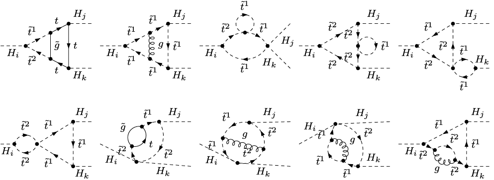
Figure 1: Sample of genuine two-loop diagrams contributing to the ${\cal O}(\alpha_{t}\alpha_{s})$ corrections to the trilinear Higgs self-couplings between $H_{i}$, $H_{j}$ and $H_{k}$ ($i,j,k=1,...,5$).

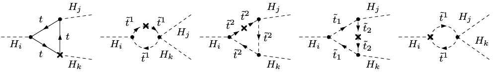
Figure 2: Some representative one-loop diagrams with one-loop counterterm insertion contributing to the ${\cal O}(\alpha_{t}\alpha_{s})$ corrections to the trilinear Higgs self-couplings.

The second part $\Delta^{\text{\tiny(}\!\text{\tiny 2}\!\text{\tiny)}}\!\lambda^{\text{CT1L}}_{\phi_{i}\phi_{j}\phi_{k}}$ denotes the contributions arising from the one-loop diagrams with top quarks and stops as loop particles and with one insertion of a counterterm of order ${\cal O}(\alpha_{s})$ from the top/stop sector. Some representative diagrams for this set are depicted in Fig. 2. The parameters of the top/stop and bottom/sbottom sectors are renormalized at order ${\cal O}(\alpha_{s})$. The bottom quarks are treated as massless, so that the left- and right-handed sbottom states do not mix and only the left-handed sbottom with a mass of $m_{\tilde{Q}_{3}}$ contributes. We choose the set of independent parameters entering the top/stop and bottom/sbottom sector, that we renormalize, to be given by

$$m_{t}\;,\quad m_{\tilde{Q}_{3}}\;,\quad m_{\tilde{t}_{R}}\quad\mbox{and}\quad A_{t}\;.$$ (2.36)

Note that $A_{t}$ is in general complex. We renormalize these parameters both in the $\overline{\text{DR}}$ and in the OS scheme. The definition of their counterterms can be found in [59]. According to the SUSY Les Houches Accord (SLHA) [93, 94] convention, $m_{\tilde{Q}_{3}}$, $m_{\tilde{t}_{R}}$ and $A_{t}$ are given as $\overline{\text{DR}}$ parameters. When we choose the OS scheme these parameters need finite shifts for the conversion into OS parameters. In the $\overline{\text{DR}}$ scheme on the other hand, the given top pole mass must be translated into a $\overline{\text{DR}}$ mass. These translations according to our conventions are described in detail in [59].

The third part consists of contributions arising from the order ${\cal O}(\alpha_{t}\alpha_{s})$ counterterms. The explicit expressions of $\Delta^{\text{\tiny(}\!\text{\tiny 2}\!\text{\tiny)}}\!\lambda^{\text{CT2L}}_{\phi_{i}\phi_{j}\phi_{k}}$ in terms of $\delta^{\text{\tiny(}\!\text{\tiny 2}\!\text{\tiny)}}\!t_{\phi}$, $\delta^{\text{\tiny(}\!\text{\tiny 2}\!\text{\tiny)}}\!M_{H^{\pm}}^{2},$ $\delta^{\text{\tiny(}\!\text{\tiny 2}\!\text{\tiny)}}\!v,$ $\delta^{\text{\tiny(}\!\text{\tiny 2}\!\text{\tiny)}}\!\tan\beta$, $\delta^{\text{\tiny(}\!\text{\tiny 2}\!\text{\tiny)}}\!|\lambda|$ and $\delta^{\text{\tiny(}\!\text{\tiny 2}\!\text{\tiny)}}\!Z_{H_{u}}$ are the same as in the one-loop case after replacing the one-loop by the two-loop counterterms. The formulae are given in Appendix C. For the exact definitions of the two-loop counterterms, we refer the reader to [59].

Our results have been obtained in two independent calculations. For the generation of the amplitudes we have employed FeynArts [95, 96] using in one calculation a model file created by SARAH [97, 68, 69, 70] and in the other calculation a model file based on the one presented in [98] which has been extended by our group to the case of the NMSSM. The contraction of the Dirac matrices was done with FeynCalc [99]. The reduction to master integrals was performed using the program TARCER [100], which is based on a reduction algorithm developed by Tarasov [101, 102] and which is included in FeynCalc. We have applied dimensional reduction [103, 104] in the manipulation of the Dirac algebra and in the tensor reduction. In our calculation no $\gamma_{5}$ terms appear that require a special treatment in $D$ dimensions, so that we take $\gamma_{5}$ to be anti-symmetric with all other Dirac matrices. The cancellation of the single pole and double poles has been checked. The results of the two computations are in full agreement. We furthermore compared our results in the limit of the real MSSM with Ref. [105] where the two-loop ${\cal O}(\alpha_{t}\alpha_{s})$ corrections to the MSSM Higgs self-couplings were given, and we found agreement between the two computations.

3 Numerical analysis

3.1 Scenarios

For the numerical analysis of the impact of the higher order corrections on the Higgs self-couplings we made sure to choose scenarios that comply with the experimental constraints. In order to find viable scenarios we performed a scan in the NMSSM parameter space. We checked the scenarios for their accordance with the LHC Higgs data by using the programs HiggsBounds [106, 107, 108] and HiggsSignals [109]. The programs require as inputs the effective couplings of the Higgs bosons, normalized to the corresponding SM values, as well as the masses, the widths and the branching ratios of the Higgs bosons. These have been obtained for the SM and NMSSM Higgs bosons from the Fortran code NMSSMCALC [74, 75]. A remark is in order for the loop-induced Higgs couplings to gluons and photons. The effective NMSSM Higgs boson coupling to the gluons normalized to the corresponding coupling of a SM Higgs boson with same mass is obtained by taking the ratio of the partial widths for the Higgs decays into gluons in the NMSSM and the SM, respectively. The QCD corrections up to next-to-next-to-next-to leading order in the limit of heavy quarks [110, 111, 112, 113, 114, 115, 116, 117, 118, 119] and squarks [120, 121] are included. As the EW corrections are unknown for the NMSSM Higgs boson decays, they are consistently neglected also in the SM decay width. The loop-mediated effective Higgs coupling to the photons has been obtained analogously. Here the NLO QCD corrections to quark and squark loops including the full mass dependence for the quarks [113, 122, 123, 124, 125, 126, 127] and squarks [128] are taken into account. The EW corrections, which are unknown for the SUSY case, are neglected also in the SM.

For the numerical analysis of the corrections to the Higgs self-couplings, we have chosen two parameter sets that fulfill the above constraints. For both scenarios we use the SM input parameters [129, 130]

$$\alpha(M_{Z}) =1/128.962\,, \alpha^{\overline{\mbox{MS}}}_{s}(M_{Z}) =0.1184\,, M_{Z} =91.1876\,~{}\text{GeV}\,,$$ (3.37)

$$M_{W} =80.385\,~{}\text{GeV}\,, m_{t} =173.5\,~{}\text{GeV}\,, m^{\overline{\text{MS}}}_{b}(m_{b}^{\overline{\text{MS}}}) =4.18\,~{}\text{GeV}\;.$$

In the numerical evaluation, however, we chose to use the running $\alpha_{s}^{\overline{\text{DR}}}$. It is obtained by converting the $\alpha^{\overline{\mbox{MS}}}_{s}$, that is evaluated with the SM renormalization group equations at two-loop order, to the $\overline{\text{DR}}$ scheme. The light quark masses, which have only a small influence on the loop results, have been set to

$$m_{u}=2.5\,~{}\text{MeV}\;,\quad m_{d}=4.95\,~{}\text{MeV}\;,\quad m_{s}=100\,~{}\text{MeV}\quad\mbox{and}\quad m_{c}=1.42\,~{}\text{GeV}\;.$$ (3.38)

The remaining parameters differ in the two scenarios. Thus we have:
Scenario 1: The soft SUSY breaking masses and trilinear couplings are chosen as

$$m_{\tilde{u}_{R},\tilde{c}_{R}}=m_{\tilde{d}_{R},\tilde{s}_{R}}=m_{\tilde{Q}_{1,2}}=m_{\tilde{L}_{1,2}}=m_{\tilde{e}_{R},\tilde{\mu}_{R}}=3\;\mbox{TeV}\,,\;m_{\tilde{t}_{R}}=1909\,~{}\text{GeV}\,,\;$$

$$m_{\tilde{Q}_{3}}=2764\,~{}\text{GeV}\,,\;m_{\tilde{b}_{R}}=1108\,~{}\text{GeV}\,,\;m_{\tilde{L}_{3}}=472\,~{}\text{GeV}\,,\;m_{\tilde{\tau}_{R}}=1855\,~{}\text{GeV}\,,$$

$$|A_{u,c,t}|=1283\,~{}\text{GeV}\,,\;|A_{d,s,b}|=1020\,~{}\text{GeV}\,,\;|A_{e,\mu,\tau}|=751\,~{}\text{GeV}\,,\;$$ (3.39)

$$|M_{1}|=908\,~{}\text{GeV},\;|M_{2}|=237\,~{}\text{GeV}\,,\;|M_{3}|=1966\,~{}\text{GeV}\,,$$

$$\varphi_{A_{d,s,b}}=\varphi_{A_{e,\mu,\tau}}=\varphi_{A_{u,c,t}}=\pi\,,\;\varphi_{M_{1}}=\varphi_{M_{2}}=\varphi_{M_{3}}=0\;.$$

The remaining input parameters are given by

$$|\lambda|=0.374\;,\quad|\kappa|=0.162\;,\quad|A_{\kappa}|=178\,~{}\text{GeV}\;,\quad|\mu_{\text{eff}}|=184\,~{}\text{GeV}\;,$$

$$\varphi_{\lambda}=\varphi_{\kappa}=\varphi_{\mu_{\text{eff}}}=\varphi_{u}=0\;,\quad\varphi_{A_{\kappa}}=\pi\;,\quad\tan\beta=7.52\;,\quad M_{H^{\pm}}=1491\,~{}\text{GeV}\;.$$ (3.40)

Scenario 2: For the soft SUSY breaking masses and trilinear couplings we chose

$$m_{\tilde{u}_{R},\tilde{c}_{R}}=m_{\tilde{d}_{R},\tilde{s}_{R}}=m_{\tilde{Q}_{1,2}}=m_{\tilde{L}_{1,2}}=m_{\tilde{e}_{R},\tilde{\mu}_{R}}=3\;\mbox{TeV}\,,\;m_{\tilde{t}_{R}}=1170\,~{}\text{GeV}\,,\;$$

$$m_{\tilde{Q}_{3}}=1336\,~{}\text{GeV}\,,\;m_{\tilde{b}_{R}}=1029\,~{}\text{GeV}\,,\;m_{\tilde{L}_{3}}=2465\,~{}\text{GeV}\,,\;m_{\tilde{\tau}_{R}}=301\,~{}\text{GeV}$$

$$|A_{u,c,t}|=1824\,~{}\text{GeV}\,,\;|A_{d,s,b}|=1539\,~{}\text{GeV}\,,\;|A_{e,\mu,\tau}|=1503\,~{}\text{GeV}\,,\;$$ (3.41)

$$|M_{1}|=862.4\,~{}\text{GeV},\;|M_{2}|=201.5\,~{}\text{GeV}\,,\;|M_{3}|=2285\,~{}\text{GeV}$$

$$\varphi_{A_{d,s,b}}=\varphi_{A_{e,\mu,\tau}}=\pi\,,\;\varphi_{A_{u,c,t}}=\varphi_{M_{1}}=\varphi_{M_{2}}=\varphi_{M_{3}}=0\;.$$

And the remaining input parameters are set as follows,

$$|\lambda|=0.629\;,\quad|\kappa|=0.208\;,\quad|A_{\kappa}|=179.7\,~{}\text{GeV}\;,\quad|\mu_{\text{eff}}|=173.7\,~{}\text{GeV}\;,$$

$$\varphi_{\lambda}=\varphi_{\mu_{\text{eff}}}=\varphi_{u}=\varphi_{A_{\kappa}}=0\;,\quad\varphi_{\kappa}=\pi\;,\quad\tan\beta=4.02\;,\quad M_{H^{\pm}}=788\,~{}\text{GeV}\;.$$ (3.42)

We follow the SLHA format, which requires $\mu_{\text{eff}}$ as input parameter. The values for $v_{s}$ and $\varphi_{s}$ can then be obtained by using Eq. (2.9). In the SLHA format, the parameters $\lambda,\kappa,A_{\kappa},\mu_{\text{eff}},\tan\beta$ as well as the soft SUSY breaking masses and trilinear couplings are understood as $\overline{\text{DR}}$ parameters at the scale $\mu_{R}=M_{s}$, whereas the charged Higgs mass is an OS parameter. We set the SUSY scale $M_{s}$ to

$$M_{s}=\sqrt{m_{\tilde{Q}_{3}}m_{\tilde{t}_{R}}}\;.$$ (3.43)

The resulting supersymmetric particle spectrum from the thus chosen parameter values is in accordance with present LHC searches for SUSY particles [131, 132, 133, 134, 135, 136, 137, 138, 139, 140, 141, 142, 143, 144, 145]. Note, that in the following we will drop the subscript ’eff’ for $\mu$. Furthermore, whenever we will use the expressions OS and $\overline{\text{DR}}$ these refer to the renormalization in the top/stop sector.

3.2 Results for the loop-corrected self-couplings

OS	${H_{1}}$	${H_{2}}$	${H_{3}}$	${H_{4}}$	${H_{5}}$
mass tree [GeV]	71.14	117.49	211.12	1491	1492
main component	$h_{u}$	$h_{s}$	$a_{s}$	$a$	$h_{d}$
mass one-loop [GeV]	98.65	139.17	217.27	1490	1491
main component	$h_{s}$	$h_{u}$	$a_{s}$	$a$	$h_{d}$
mass two-loop [GeV]	94.68	125.06	217.32	1490	1491
main component	$h_{s}$	$h_{u}$	$a_{s}$	$a$	$h_{d}$
$\overline{\text{DR}}$	${H_{1}}$	${H_{2}}$	${H_{3}}$	${H_{4}}$	${H_{5}}$
mass tree [GeV]	71.14	117.49	211.12	1491	1492
main component	$h_{u}$	$h_{s}$	$a_{s}$	$a$	$h_{d}$
mass one-loop [GeV]	91.60	120.00	217.36	1491	1491
main component	$h_{s}$	$h_{u}$	$a_{s}$	$a$	$h_{d}$
mass two-loop [GeV]	94.41	124.24	217.33	1490	1491
main component	$h_{s}$	$h_{u}$	$a_{s}$	$a$	$h_{d}$

Table 1: Scenario 1: Masses and main components of the neutral Higgs bosons at tree and one-loop level and at order ${\cal O}(\alpha_{t}\alpha_{s})$ as obtained by using OS (upper) and $\overline{\text{DR}}$ (lower) renormalization in the top/stop sector.

In this and the following subsection we discuss the impact of the order ${\cal O}(\alpha_{t}\alpha_{s})$ corrections on the trilinear Higgs self-couplings and on Higgs-to-Higgs decay widths. We start by discussing the results for the parameter set called scenario 1 in the previous subsection. The masses of the Higgs bosons and their main composition in terms of singlet/doublet and scalar/pseudoscalar components at tree level, one-loop and two-loop order are summarized in Table 1 both for the OS and the $\overline{\text{DR}}$ renormalization in the top/stop sector. The tree-level stop masses in this scenario are rather heavy and given by

$$\begin{array}[]{llll}\mbox{OS}&:&m_{\tilde{t}_{1}}=1992\mbox{ GeV}\;,&m_{\tilde{t}_{2}}=2820\mbox{ GeV}\;,\\ \overline{\text{DR}}&:&m_{\tilde{t}_{1}}=1911\mbox{ GeV}\;,&m_{\tilde{t}_{2}}=2768\mbox{ GeV}\;.\end{array}$$ (3.46)

and for the $\overline{\text{DR}}$ top mass we have $m_{t}^{\overline{\text{DR}}}=136.34$ GeV. For definiteness, with respect to the mass corrections one-loop means here and in the following that we include the full EW corrections at non-vanishing external momenta, while at two-loop level the order ${\cal O}(\alpha_{t}\alpha_{s})$ corrections are computed at vanishing external momenta. As can be inferred from the table, the masses of the three lightest scalars are substantially different, so that mixing effects due to CP-violation for non-vanishing phases cannot be expected to be significant. The reason for choosing this scenario are higher order corrections to the trilinear Higgs self-coupling of the SM-like Higgs boson which are rather important for this parameter point. This boson is given by the state with the largest $h_{u}$ component and a mass value around 125 GeV. At tree level it is the lightest Higgs boson $H_{1}$ that is mainly $h_{u}$-like, and its mass thus receives large corrections which are dominantly stemming from the top/stop sector. The large corrections shift the $H_{1}$ mass above the one of $H_{2}$ so that the two Higgs bosons interchange their roles, as they are ordered by ascending mass. At one- and two-loop level it is therefore the second lightest Higgs boson, which is $h_{u}$-like. For convenience, we denote in the following the mass eigenstate that is dominantly $h_{u}$-like, by $h$. Furthermore, when we perform comparisons in the interaction basis at different loop-levels, these will be done for the $h_{u}$ state.

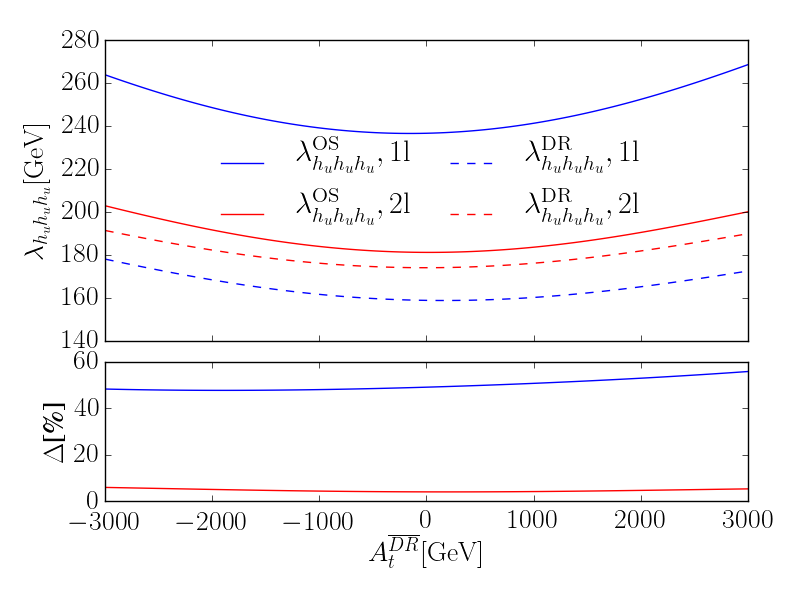
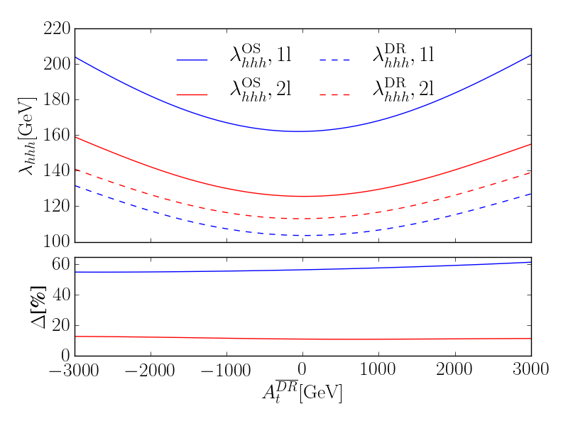
Figure 3: Scenario 1: Upper panels: Trilinear self-coupling of the $h_{u}$ interaction state (left) and the mass eigenstate $h$ (right) as a function of $A_{t}^{\overline{\text{DR}}}$ including the one-loop correction (blue/two outer lines) and also the two-loop corrections (red/two middle lines). In the top/stop sector either the OS scheme (solid lines) or the $\overline{\mbox{DR}}$ scheme (dashed lines) has been applied. Lower Panels: Absolute value of the relative deviation of the correction using OS or ${\overline{\mbox{DR}}}$ renormalization in the top/stop sector, $\Delta=|\lambda_{HHH}^{m_{t}(\overline{\text{DR}})}-\lambda_{HHH}^{m_{t}\text{(OS)}}|/\lambda_{HHH}^{m_{t}(\overline{\text{DR}})}$ ($H=h_{u},h$), in percent as a function of $A_{t}^{\overline{\text{DR}}}$, at one-loop (blue/upper) and two-loop (red/lower).

In Fig. 3 we show the dependence of the one- and two-loop corrections to the Higgs self-coupling on the $\overline{\text{DR}}$ parameter $A_{t}$ in the two different renormalization schemes applied in the stop sector. The one-loop corrections have been obtained at order ${\cal O}(\alpha_{t})$ for vanishing external momenta. We explicitly verified, that the differences between the one-loop result in this approximation and the one including the full one-loop corrections for non-vanishing momenta at the threshold are below 4% for the investigated parameter points. Two-loop corrections always refer to the order ${\cal O}(\alpha_{t}\alpha_{s})$ corrections at vanishing external momenta. The left plot of Fig. 3 shows the corrections to the self-coupling of $h_{u}$ in the interaction basis, $\lambda_{h_{u}h_{u}h_{u}}$. Figure 3 (right) displays the loop-corrected self-couplings after rotation to the mass eigenstate $h$ with dominant $h_{u}$ component. The rotation to the mass eigenstates is performed with the mixing matrix ${\cal R}^{(2)}$ defined in Eq. (2.5) for both the one- and the two-loop curves in the plot. The mass values and mixing matrix elements have been computed with NMSSMCALC. Note that at two-loop order the $h_{u}$ dominated state is given by the second lightest Higgs boson $H_{2}$, cf. Table 1. The dependence on $A_{t}$ is more pronounced after rotation to the mass eigenstates. Overall, however, the size and shape of the corrections both in the interaction and in the mass eigenstates are comparable. At the parameter point of scenario 1 the tree-level coupling $\lambda_{h_{u}h_{u}h_{u}}=101.70$ GeV in both renormalization schemes. In the OS scheme the one-loop correction increases it by 140% while it is decreased by 24% to two-loop order. In the $\overline{\text{DR}}$ scheme the increase is of 74% going from tree- to one-loop order supplemented by another increase of 9% when adding the two-loop corrections. The reason, why the one- and two-loop corrections differ much more in the OS scheme than in the $\overline{\mbox{DR}}$ scheme can be understood as follows. In the $\overline{\mbox{DR}}$ scheme the top quark mass, which according to the SLHA accord is an OS parameter, has to be converted to the $\overline{\mbox{DR}}$ value. Thereby, the finite counterterm to the top mass, which in the OS scheme is included at two-loop level, is already induced at one-loop level in the value of the $\overline{\mbox{DR}}$ mass. In this way some corrections of order ${\cal O}(\alpha_{t}\alpha_{s})$, which in the OS scheme only appear at the two-loop level, are moved to the one-loop level, cf. also [59].

The lower panels of Fig. 3 display the difference in the self-couplings when using the two different renormalization schemes in the top/stop sector,

$$\Delta=\frac{|\lambda_{HHH}^{m_{t}(\overline{\text{DR}})}-\lambda_{HHH}^{m_{t}\text{(OS)}}|}{\lambda_{HHH}^{m_{t}(\overline{\text{DR}})}}\;,$$ (3.47)

where $H$ both refers to the $h_{u}$ dominated mass eigenstate $h$, and to the $h_{u}$ interaction eigenstate. This value gives a rough estimate of the theoretical error in the Higgs self-coupling due to the unknown higher order corrections. In the interaction eigenstate it is of order ${\cal O}(50\%)$ at one-loop level, decreasing to roughly 4% at two-loop level. In the mass eigenstate it is about 5% higher at both loop orders. The inclusion of the two-loop corrections hence substantially decreases the theoretical uncertainty.

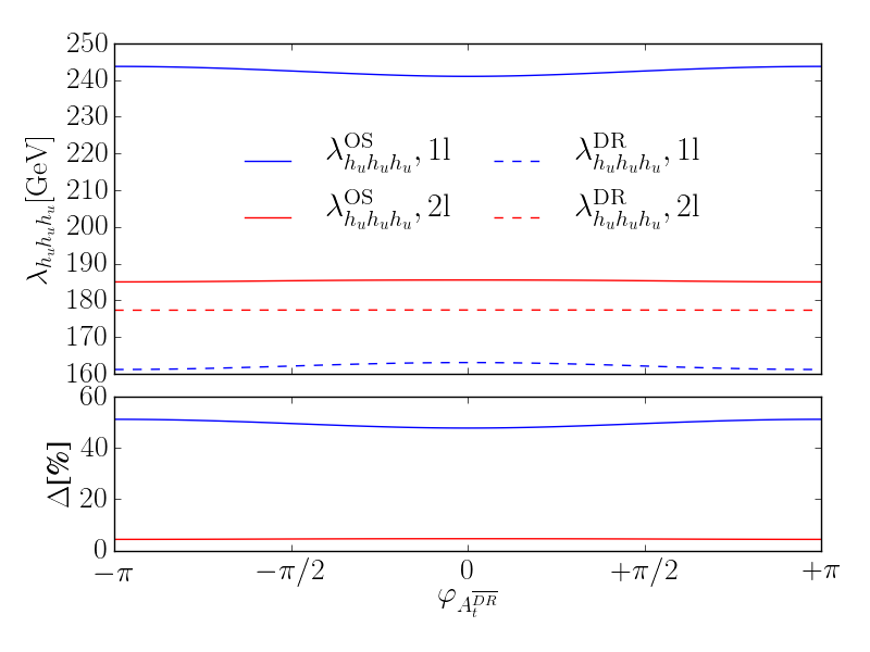
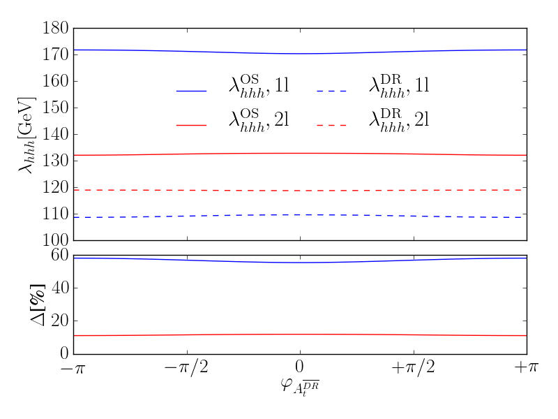
Figure 4: Scenario 1: Same as Fig. 3, but now as a function of $\varphi_{A_{t}}^{\overline{\text{DR}}}$.

Figure 4 shows the same as Fig. 3 but now as a function of the phase $\varphi_{A_{t}}$. All other CP-violating phases have been kept to zero. The figure shows that the dependence of the loop corrections on the phase is almost negligible, as expected for radiatively induced CP-violation. The size of the loop corrections and the remaining theoretical uncertainty are of the same order as for the variation of $A_{t}$.

OS	${H_{1}}$	${H_{2}}$	${H_{3}}$	${H_{4}}$	${H_{5}}$
mass tree [GeV]	79.15	103.55	146.78	796.62	803.86
main component	$h_{s}$	$h_{u}$	$a_{s}$	$h_{d}$	$a$
mass one-loop [GeV]	103.45	129.15	139.83	796.53	802.94
main component	$h_{s}$	$a_{s}$	$h_{u}$	$h_{d}$	$a$
mass two-loop [GeV]	102.99	126.09	128.94	796.45	803.07
main component	$h_{s}$	$h_{u}$	$a_{s}$	$h_{d}$	$a$
$\overline{\text{DR}}$	${H_{1}}$	${H_{2}}$	${H_{3}}$	${H_{4}}$	${H_{5}}$
mass tree [GeV]	79.15	103.55	146.78	796.62	803.86
main component	$h_{s}$	$h_{u}$	$a_{s}$	$h_{d}$	$a$
mass one-loop [GeV]	102.80	120.52	128.80	796.36	803.09
main component	$h_{s}$	$h_{u}$	$a_{s}$	$h_{d}$	$a$
mass two-loop [GeV]	103.09	124.55	128.91	796.36	803.03
main component	$h_{s}$	$h_{u}$	$a_{s}$	$h_{d}$	$a$

Table 2: Scenario 2: Masses and main components of the neutral Higgs bosons at tree and one-loop level and at order ${\cal O}(\alpha_{t}\alpha_{s})$ as obtained by using OS (upper) and $\overline{\text{DR}}$ (lower) renormalization in the top/stop sector.

We now turn to the discussion of scenario 2. The masses and dominant composition of the mass eigenstates at tree level, one- and two-loop order are summarized in Table 2. In the OS scheme again the composition of the mass ordered states changes when going from tree level to one-loop level and from one- to two-loop level. In contrast to scenario 1 the masses of $H_{2}$ and $H_{3}$ are now much closer together, in particular after inclusion of the two-loop corrections. We therefore expect CP-violating effects to be more important here. The $H_{2}$ state is identified with the discovered Higgs boson. The stop masses are again rather heavy with

$$\begin{array}[]{llll}\mbox{OS}&:&m_{\tilde{t}_{1}}=1145\mbox{ GeV}\;,&m_{\tilde{t}_{2}}=1421\mbox{ GeV}\;,\\ \overline{\text{DR}}&:&m_{\tilde{t}_{1}}=1126\mbox{ GeV}\;,&m_{\tilde{t}_{2}}=1387\mbox{ GeV}\;.\end{array}$$ (3.50)

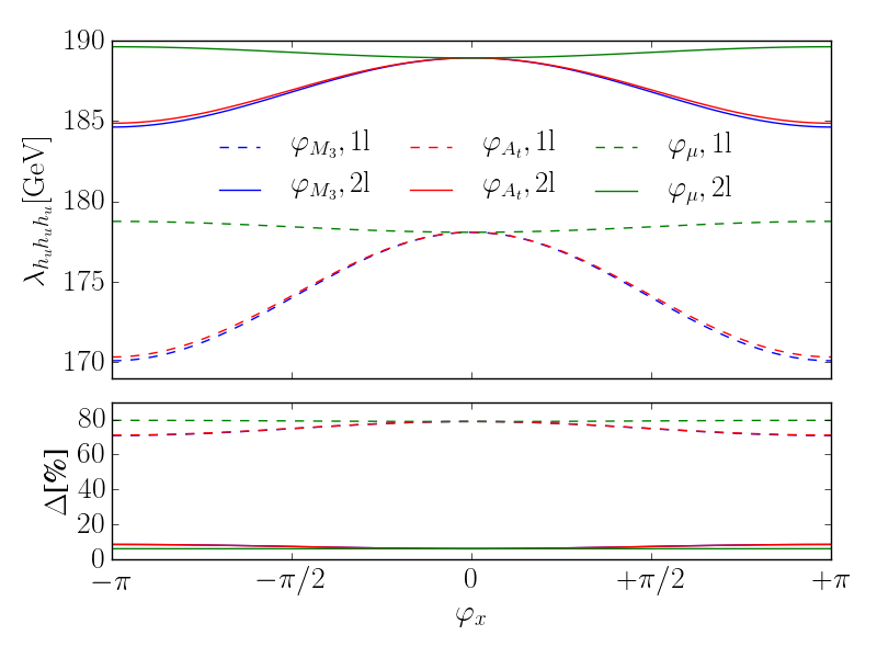
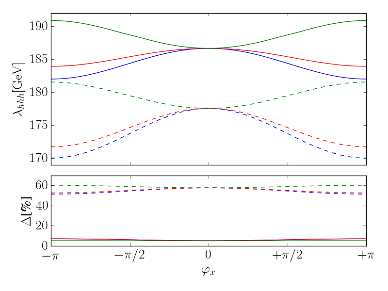
Figure 5: Scenario 2: Upper panels: Trilinear self-coupling of the $h_{u}$ interaction state (left) and the mass eigenstate $h$ (right) at one-loop (dashed lines) and two-loop (solid lines) as a function of the phases $\varphi_{\mu}$ (green/grey), $\varphi_{A_{t}}$ (red/black upper) and $\varphi_{M_{3}}$ (blue/black lower). Lower Panels: Size of the relative correction of $n^{th}$ order to the Higgs self-coupling with respect to the $(n-1)^{th}$ order – i.e. $\Delta=|\lambda_{HHH}^{(n)}-\lambda_{HHH}^{(n-1)}|/\lambda_{HHH}^{(n-1)}$ – in percent for $H=h_{u}$ (left) and $H=h$ (right) as a function of the phases $\varphi_{\mu}$ (green/grey), $\varphi_{A_{t}}$ (red/black) and $\varphi_{M_{3}}$ (blue/black) for $n=2$ (solid line) and $n=1$ (dashed line). The red and blue lines almost lie on top of each other. In the top/stop sector we have applied $\overline{\text{DR}}$ renormalization.

In Fig. 5 we show the dependence of the Higgs self-coupling of the $h_{u}$ state in the interaction basis (left) and of the $h_{u}$-like mass eigenstate $h$ (right) at one- (dashed) and two-loop order (full) for $\overline{\text{DR}}$ renormalization in the top/stop sector as a function of the phases $\varphi_{M_{3}}$, $\varphi_{A_{t}}$ and $\varphi_{\mu}$. For illustrative purposes we have varied the phases in rather large ranges although they might already be excluded by experiment. We start from our original CP-conserving scenario and turn on the phases one by one. Note, that $\varphi_{\mu}$ has been varied such that the CP-violating phase $\varphi_{y}=\varphi_{\kappa}-\varphi_{\lambda}+2\varphi_{s}-\varphi_{u}$, that appears already at tree level in the Higgs sector, remains zero, i.e. $\varphi_{\lambda}$ and $\varphi_{s}$ were varied at the same time as $\varphi_{\lambda}=2\varphi_{s}=2/3\varphi_{\mu}$, while $\varphi_{\kappa}$ and $\varphi_{u}$ are kept zero. As expected, the loop-corrected couplings show a somewhat larger dependence on $\varphi_{A_{t}}$ than in scenario 1, in particular in the mass eigenstate basis. Defining as

$$\delta\lambda_{HHH}=\frac{\lambda_{HHH}(\pi)-\lambda_{HHH}(0)}{\lambda_{HHH}(0)}\;,$$ (3.51)

we have in the mass eigenstate basis $H\equiv h$ the variations

$$\delta\lambda_{hhh}^{\varphi_{\mu}}=2.2\%\;,\quad\delta\lambda_{hhh}^{\varphi_{A_{t}}}=1.6\%\quad\mbox{and}\quad\delta\lambda_{hhh}^{\varphi_{M_{3}}}=2.7\%$$ (3.52)

for the two-loop corrected self-coupling. Note, that the one-loop corrected self-couplings show a dependence on the phase of $M_{3}$, although the genuine diagrammatic gluino corrections only appear at two-loop level. This dependence enters through the conversion of the OS top quark mass to the $\overline{\mbox{DR}}$ mass. Overall, the dependence of the loop corrected self-couplings on the CP-violating phases is smaller in the interaction states than in the mass eigenstates, which are obtained by rotating the interaction states with the mixing elements obtained from the loop corrected masses, that also depend on the CP-violating phases.

The lower panels show the relative corrections, defined at order $n=1,2$ as

$$\Delta=\frac{|\lambda_{HHH}^{(n)}-\lambda_{HHH}^{(n-1)}|}{\lambda_{HHH}^{(n-1)}}\;.$$ (3.53)

In the interaction basis they are of order $\sim 70-80$% for the one-loop corrections relative to the tree-level coupling and are somewhat larger than the corresponding values in the mass eigenstate basis, which are of order $\sim 50-60$%. For the two-loop coupling relative to the one-loop coupling the corrections are significantly reduced to about $5-8$% in both the interaction and the mass eigenstate basis. The two-loop corrections hence considerably reduce the theoretical uncertainty.

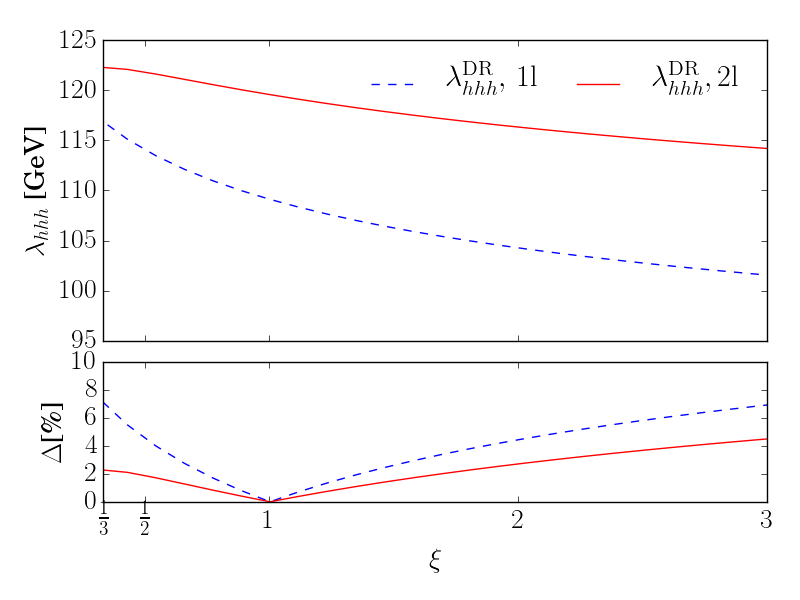
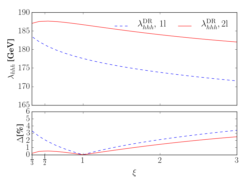
Figure 6: Scale dependence of the trilinear coupling $\lambda_{hhh}$ at one- (blue/dashed) and two-loop order (red/full) for scenario 1 (left) and scenario 2 (right). The scale $\mu_{R}=\xi M_{s}$ has been varied in an interval of $\xi=1/3...3$ around the central scale $\mu_{0}=M_{s}$. The lower plots show the variation in percent compared to the central scale, i.e. $\Delta=[\lambda_{hhh}(\mu_{R})-\lambda_{hhh}(\mu_{0})]/\lambda_{hhh}(\mu_{0})$.

In order to further study the theoretical uncertainty, we show in Fig. 6 for scenario 1 (left) and scenario 2 (right) the scale variation of the trilinear Higgs self-coupling in the mass eigenstate $h$ at one- and at two-loop order. We have varied the renormalization scale $\mu_{R}$ between 1/3 and 3 times the central scale $\mu_{0}=M_{s}$. The scale variation affects the $\overline{\mbox{DR}}$ parameters entering the calculation. In the absence of an implementation of the 2-loop renormalization group equations (RGE) for the complex NMSSM, which is devoted to future work, we obtain the parameters at the different scales by exploiting the relation between $\overline{\mbox{DR}}$ and OS parameters, as explained in Appendix D. This should approximate the results obtained from the RGE running rather well, in case the scale is not varied in a too large range. Since the scale variation provides only a rough estimate of the error made by neglecting higher order corrections this approach is sufficient for our purpose. As can be inferred from the figures, in scenario 1 the one-loop coupling is altered by up to 7% compared to its value at the central scale in the investigated range. This reduces to 2-5% at two-loop order. In scenario 2 the corresponding numbers at one-loop order are 3.5% compared to up to 2.5% for the two-loop coupling. As expected, the scale dependence reduces when going from one- to two-loop order. Note, however, that these numbers should not be taken as estimate for the residual theoretical uncertainty.

3.3 Phenomenological implications

We now turn to the discussion of the phenomenological implications due to the loop-corrected Higgs self-couplings. Higgs self-couplings are involved in Higgs-to-Higgs decays and in Higgs pair production processes. At the LHC, pair production dominantly proceeds through gluon fusion. This process, however, includes EW corrections beyond those approximated by the loop-corrected effective trilinear couplings. As they are not available at present we will not discuss Higgs pair production further and concentrate on Higgs-to-Higgs decays.

The decay width for the Higgs-to-Higgs decay $H_{i}\to H_{j}H_{k}$ including the two-loop corrections to the Higgs self-coupling is obtained from

$$\Gamma(H_{i}\to H_{j}H_{k})=\frac{\lambda^{1/2}(M_{H_{i}}^{2},M_{H_{j}}^{2},M_{H_{k}}^{2})}{16\pi f\,M_{H_{i}}^{3}}|{\cal M}_{H_{i}\to H_{j}H_{k}}|^{2}\;,$$ (3.54)

where $f=2$ for identical final state particles and $f=1$ otherwise. The decay amplitude is denoted by ${\cal M}_{H_{i}\to H_{j}H_{k}}$ and $\lambda=(x-y-z)^{2}-4yz$ is the two-body phase space function. In case of CP-violation all Higgs-to-Higgs decays between the five neutral Higgs bosons are possible, if kinematically allowed, so that $i,j,k=1,...,5$. In the CP-conserving case, however, only the trilinear Higgs couplings between three CP-even or one CP-even and two CP-odd Higgs bosons are non-vanishing. The matrix element is given by

$${\cal M}_{H_{i}\to H_{j}H_{k}} = \sum_{i^{\prime},j^{\prime},k^{\prime}=1}^{5}{\bf Z}_{ii^{\prime}}{\bf Z}_{jj^{\prime}}{\bf Z}_{kk^{\prime}}\Gamma_{h_{i^{\prime}}h_{j^{\prime}}h_{k^{\prime}}}+\delta M_{H_{i}\to H_{j}H_{k}}^{\text{mix}}\;.$$ (3.55)

Here $\Gamma_{h_{i^{\prime}}h_{j^{\prime}}h_{k^{\prime}}}$ is the loop corrected trilinear Higgs self-coupling in the tree-level mass eigenstate basis, where the Goldstone boson has been singled out. We here include at one-loop level the full electroweak corrections [79] at $p^{2}\neq 0$, where we set the 4-momenta of the external Higgs particles equal to the respective loop-corrected Higgs mass values $p_{H_{i,j,k}}^{2}=M_{H_{i,j,k}}^{2}$ as obtained with NMSSMCALC [51, 58, 59, 75], and at two-loop the order ${\cal O}(\alpha_{t}\alpha_{s})$ corrections at $p^{2}=0$. The proper on-shell conditions of the external Higgs bosons as required in the decay process are ensured by rotating the tree-level mass eigenstates $h_{i^{\prime},j^{\prime},k^{\prime}}$ to the loop corrected mass eigenstates $H_{i,j,k}$ with the matrix ${\bf Z}$, cf. [51, 79]. In this calculation we include at one-loop order the full electroweak corrections at non-vanishing external momenta. At two-loop order as usual the order ${\cal O}(\alpha_{t}\alpha_{s})$ corrections which are available only at $p^{2}=0$ are taken into account. The $\delta M_{H_{i}\to H_{j}H_{k}}^{\text{mix}}$ accounts for the contributions stemming from the mixing of the CP-odd components of the external Higgs bosons with the Goldstone and with the $Z$ boson, respectively. These contributions, which are evaluated by setting the external momenta to the tree-level masses in order to maintain gauge invariance, are small already at one-loop order compared to the remaining contributions to the decay amplitude, as has been shown in [79]. We hence do not include the two-loop contributions, that can safely be expected to be negligible.

In the plots below we show apart from the two-loop corrected decay widths also the ones at one-loop order. The only change required to adapt formula (3.55) to this case is in $\Gamma_{h_{i^{\prime}}h_{j^{\prime}}h_{k^{\prime}}}$ where solely the one-loop corrections to the vertex functions together with the corresponding counterterms are included. In particular we also use the two-loop corrected mass eigenstates and mixing matrix elements for the external particles (apart from the mixing contribution with the Goldstone and $Z$ boson of course).

The scenario which the following discussion is based on and which has been checked to be compatible with the constraints from the LHC Higgs data, is given by:

Scenario 3: The soft SUSY breaking masses and trilinear couplings are chosen as

$$m_{\tilde{u}_{R},\tilde{c}_{R}}=m_{\tilde{d}_{R},\tilde{s}_{R}}=m_{\tilde{Q}_{1,2}}=m_{\tilde{L}_{1,2}}=m_{\tilde{e}_{R},\tilde{\mu}_{R}}=3\;\mbox{TeV}\,,\;m_{\tilde{t}_{R}}=1940\,~{}\text{GeV}\,,\;$$

$$m_{\tilde{Q}_{3}}=2480\,~{}\text{GeV}\,,\;m_{\tilde{b}_{R}}=1979\,~{}\text{GeV}\,,\;m_{\tilde{L}_{3}}=2667\,~{}\text{GeV}\,,\;m_{\tilde{\tau}_{R}}=1689\,~{}\text{GeV}\,,$$

$$|A_{u,c,t}|=1192\,~{}\text{GeV}\,,\;|A_{d,s,b}|=685\,~{}\text{GeV}\,,\;|A_{e,\mu,\tau}|=778\,~{}\text{GeV}\,,\;$$ (3.56)

$$|M_{1}|=517\,~{}\text{GeV},\;|M_{2}|=239\,~{}\text{GeV}\,,\;|M_{3}|=1544\,~{}\text{GeV}\,,$$

$$\varphi_{A_{d,s,b}}=\varphi_{A_{e,\mu,\tau}}=0\,,\;\varphi_{A_{u,c,t}}=\pi\,,\;\varphi_{M_{1}}=\varphi_{M_{2}}=\varphi_{M_{3}}=0\;.$$

The remaining input parameters are given by

$$|\lambda|=0.267\;,\quad|\kappa|=0.539\;,\quad|A_{\kappa}|=810\,~{}\text{GeV}\;,\quad|\mu_{\text{eff}}|=104\,~{}\text{GeV}\;,$$

$$\varphi_{\lambda}=\varphi_{\kappa}=\varphi_{\mu_{\text{eff}}}=\varphi_{u}=0\;,\quad\varphi_{A_{\kappa}}=\pi\;,\quad\tan\beta=8.97\;,\quad M_{H^{\pm}}=613\,~{}\text{GeV}\;.$$ (3.57)

This results in the Higgs mass spectrum given in Table 3 at tree, one- and two-loop level together with the main singlet/doublet and scalar/pseudoscalar components at each loop level.

OS	${H_{1}}$	${H_{2}}$	${H_{3}}$	${H_{4}}$	${H_{5}}$
mass tree [GeV]	49.17	99.83	609.21	611.77	715.92
main component	$h_{s}$	$h_{u}$	$a$	$h_{d}$	$a_{s}$
mass one-loop [GeV]	87.36	139.10	608.71	611.37	694.73
main component	$h_{s}$	$h_{u}$	$a$	$h_{d}$	$a_{s}$
mass two-loop [GeV]	83.66	124.95	608.73	611.37	694.76
main component	$h_{s}$	$h_{u}$	$a$	$h_{d}$	$a_{s}$
$\overline{\text{DR}}$	${H_{1}}$	${H_{2}}$	${H_{3}}$	${H_{4}}$	${H_{5}}$
mass tree [GeV]	49.17	99.83	609.21	611.77	715.92
main component	$h_{s}$	$h_{u}$	$a$	$h_{d}$	$a_{s}$
mass one-loop [GeV]	80.66	119.68	608.72	611.37	694.79
main component	$h_{s}$	$h_{u}$	$a$	$h_{d}$	$a_{s}$
mass two-loop [GeV]	83.03	124.34	608.71	611.36	694.78
main component	$h_{s}$	$h_{u}$	$a$	$h_{d}$	$a_{s}$

Table 3: Scenario 3: Masses and main components of the neutral Higgs bosons at tree and one-loop level and at order ${\cal O}(\alpha_{t}\alpha_{s})$ as obtained by using OS (upper) and $\overline{\text{DR}}$ (lower) renormalization in the top/stop sector.

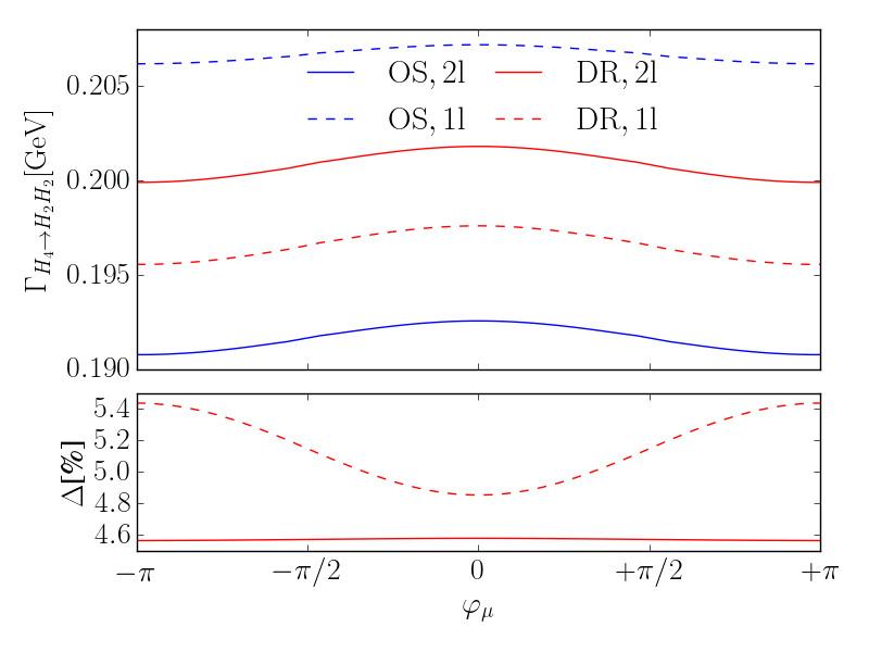
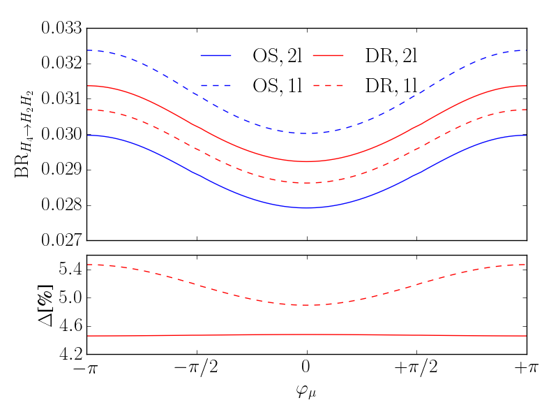
Figure 7: Scenario 3: Upper: Loop-corrected decay width (left) and branching ratio (right) of the Higgs-to-Higgs decay $H_{4}\to H_{2}H_{2}$ as a function of $\varphi_{\mu}$ with the top/stop sector renormalized in the OS (blue/two outer lines) and in the $\overline{\mbox{DR}}$ scheme (red/two inner lines) at 1-loop (dashed) and at 2-loop (full) order. Lower: Relative deviation between the two renormalization schemes $\Delta=|O(\overline{\mbox{DR}})-O(\mbox{OS})|/O(\overline{\mbox{DR}})$ for $O=\Gamma$ (left) and $O=\mbox{BR}$ (right) at 1-loop (dashed) and 2-loop (full).

In Fig. 7 (left) we show the partial decay width for the decay of the heavy $h_{d}$-like Higgs boson $H_{4}$ into a pair of SM-like Higgs bosons $H_{2}$, including the higher order corrections to the Higgs-self-couplings at one- and two-loop level as obtained from Eq. (3.54). We start from the parameter point of scenario 3 with vanishing phase $\varphi_{\mu}=0$. The phase is then varied in the range $-\pi...\pi$, such that at tree level the CP-violating phase $\varphi_{y}$ in the Higgs sector vanishes. As expected the dependence of the decay width on the CP-violating phase induced through the loop corrections is small, remaining below the per-cent level. For $\varphi_{\mu}=0$ the tree-level decay width in the OS scheme is 0.171 GeV and 0.186 GeV in the $\overline{\mbox{DR}}$ scheme. In the latter the one-loop corrections increase the decay width by 6.5% and the two-loop corrections add another 2.0% on top of that. In the OS we find a 21% increase at one-loop and a 7% decrease at two-loop so that at two-loop order the results in the two renormalization schemes approach each other, as can also be inferred from the lower left plot, which shows that the dependence on the renormalization scheme decreases from one- to two-loop level. Depending on the renormalization scheme different input parameters of the top/stop sector have to be converted to match the required renormalization scheme. The corresponding induced two-loop corrections into the one-loop corrections lead to a different dependence on the CP-violating phase of the two schemes at one-loop level. At two-loop level this difference in the phase dependence is then almost washed out and the scheme dependence is about 4.58% independent of $\varphi_{\mu}$. For the computation of the branching ratio of the decay, shown in Fig. 7 (right), we replace in the program package NMSSMCALC the tree-level decay widths $\Gamma(H_{i}\to H_{j}H_{k})$ with our loop-corrected ones. The branching ratio, which with ${\cal O}(3\%)$ is very small shows the same trend as the decay width with respect to the loop corrections.

The non-vanishing CP-violating phase induces through the higher order corrections CP mixing in the Higgs mass eigenstates, such that otherwise not allowed decays of e.g. the CP-odd doublet-like $H_{3}$ into a pair of SM-like $H_{2}$ bosons are possible. The branching ratio remains, however, tiny, reaching at most 0.58 per mille for $|\varphi_{\mu}|\approx\pi/2$ in our scenario.

4 Conclusions

The search for New Physics and the proper interpretation of the experimental data requires from the theoretical side precise predictions of parameters and observables. In this work we computed the two-loop corrections to the trilinear Higgs self-couplings in the CP-violating NMSSM. Originating from the Higgs potential the Higgs boson masses and self-couplings are related to each other. For a consistent interpretation therefore the level of accuracy of the self-couplings has to match the one of the masses, that have been provided previously up to the two-loop level. Here, the two-loop corrections to the self-couplings have been calculated at the same order ${\cal O}(\alpha_{t}\alpha_{s})$ at vanishing external momenta. We have allowed for two renormalization schemes in the top/stop sector, namely OS and $\overline{\text{DR}}$ renormalization. Depending on the scenario and the renormalization scheme, the two-loop corrections are of the order of 5-10% relative to the one-loop couplings, compared to up to 80% for the one-loop corrections relative to the tree-level values. The investigation of the remaining theoretical uncertainty performed by varying the renormalization scheme of the top/stop sector or by changing the renormalization scale confirmed that the theoretical error is reduced through the inclusion of the two-loop corrections. As expected the dependence on the CP-violating phase due to radiatively induced CP-violation is small and of the order of a few percent.

The trilinear self-couplings are relevant in Higgs pair production processes and Higgs-to-Higgs decays, which now become accessible at run 2 of the LHC. While Higgs pair production requires the inclusion of further higher order corrections beyond the loop-corrected Higgs self-couplings provided in this work, the inclusion of the radiatively corrected trilinear Higgs self-coupling improves the prediction for the Higgs-to-Higgs decay rates and related branching ratios. For the investigated scenario and decay we find that the two-loop corrections alter the decay width by 2% (7%) in the $\overline{\text{DR}}$ (OS) scheme with respect to the one-loop level, which is to be compared to about 7% (21%) when going from tree- to one-loop level. The dependence on the renormalization scheme is reduced from $\sim 4.8-5.4$% in the investigated range of the phase $\varphi_{\mu}$ at one-loop level to $\sim 4.5$% at two-loop level. The behaviour in the branching ratio is similar to the one of the decay width.

In summary, the inclusion of the two-loop corrections at ${\cal O}(\alpha_{t}\alpha_{s})$ in the approximation of vanishing external momenta in the trilinear Higgs self-couplings of the CP-violating NMSSM Higgs sector is necessary to match the available precision in the Higgs masses and to allow for a consistent interpretation of the Higgs data. Being of the order of 10% they have been shown to further reduce the theoretical error due to missing higher order corrections.

Acknowledgments

MM and DTN have been supported in part by the DFG SFB/TR9 “Computational Particle Physics”. HZ acknowledges financial support from the Graduiertenkolleg “GRK 1694: Elementarteilchenphysik bei höchster Energie und höchster Präzision”. The authors thank Michael Spira and Kathrin Walz for helpful discussions.

Appendix

Appendix A Tree-level trilinear Higgs self-couplings

In this appendix we present the tree-level trilinear Higgs self-couplings in the interaction eigenstates, $\lambda_{ijk},$ $i,j,k=1,...,6$ with the correspondences $1\mathrel{\widehat{=}}h_{d}$, $2\mathrel{\widehat{=}}h_{u}$, $3\mathrel{\widehat{=}}h_{s}$, $4\mathrel{\widehat{=}}a_{d}$, $5\mathrel{\widehat{=}}a_{u}$, $6\mathrel{\widehat{=}}a_{s}$. They are symmetric in the three indices. Using the short-hand notations $c_{x}\equiv\cos x$ etc. and

$$\phi_{x} = \varphi_{u}+\varphi_{s}+\varphi_{\lambda}+\varphi_{A_{\lambda}}\,,$$

$$\phi_{y} = \varphi_{u}-2\varphi_{s}+\varphi_{\lambda}-\varphi_{\kappa}\,,$$ (A.58)

$$\phi_{z} = 3\varphi_{s}+\varphi_{A_{\kappa}}+\varphi_{\kappa}\,,$$

we have

$$\lambda_{111} =\frac{3c_{\beta}M_{Z}^{2}}{v}\,,\quad\lambda_{112}=-\frac{s_{\beta}M_{Z}^{2}}{v}+|\lambda|^{2}s_{\beta}v\,,\quad\lambda_{113}=|\lambda|^{2}v_{s}\,,\quad\lambda_{114}=0\,,\quad\lambda_{115}=0\,,$$

$$\lambda_{116} =0\,,\quad\lambda_{122}=-\frac{c_{\beta}M_{Z}^{2}}{v}+|\lambda|^{2}c_{\beta}v\,,\quad\lambda_{123}=-\frac{|A_{\lambda}||\lambda|c_{\phi_{x}}}{\sqrt{2}}-|\lambda||\kappa|v_{s}c_{\phi_{y}}\,,\quad\lambda_{124}=0\,,$$

$$\lambda_{125} =0\,,\quad\lambda_{126}=-\frac{3}{2}|\lambda||\kappa|v_{s}s_{\phi_{y}}\,,\quad\lambda_{133}=|\lambda|^{2}vc_{\beta}-|\kappa||\lambda|vs_{\beta}c_{\phi_{y}}\,,\quad\lambda_{134}=0\,,$$

$$\lambda_{135} =\frac{1}{2}|\lambda||\kappa|v_{s}s_{\phi_{y}}\,,\quad\lambda_{136}=-|\lambda||\kappa|vs_{\phi_{y}}s_{\beta}\,,\quad\lambda_{144}=\frac{c_{\beta}M_{Z}^{2}}{v}\,,\quad\quad\lambda_{145}=0\,,$$

$$\lambda_{146} =0\,,\quad\lambda_{155}=-\frac{c_{\beta}M_{Z}^{2}}{v}+|\lambda|^{2}c_{\beta}v\,,\quad\lambda_{156}=\frac{|A_{\lambda}||\lambda|c_{\phi_{x}}}{\sqrt{2}}-|\lambda||\kappa|v_{s}c_{\phi_{y}}\,,$$

$$\lambda_{166} =|\lambda|^{2}c_{\beta}v+|\kappa||\lambda|vs_{\beta}c_{\phi_{y}}\,,\quad\lambda_{222}=\frac{3M_{Z}^{2}s_{\beta}}{v}\,,\quad\lambda_{223}=|\lambda|^{2}v_{s}\,,\quad\lambda_{224}=0\,,\quad\lambda_{225}=0\,,$$

$$\lambda_{226} =0\,,\quad\lambda_{233}=-|\lambda||\kappa|vc_{\beta}c_{\phi_{y}}+|\lambda|^{2}s_{\beta}v\,,\quad\lambda_{234}=\frac{1}{2}|\kappa||\lambda|v_{s}s_{\phi_{y}}\,,\quad\lambda_{235}=0\,,$$

$$\lambda_{236} =-|\kappa||\lambda|vc_{\beta}s_{\phi_{y}}\,,\quad\lambda_{244}=-\frac{M_{Z}^{2}s_{\beta}}{v}+|\lambda|^{2}vs_{\beta}\,,\quad\lambda_{245}=0\,,$$

$$\lambda_{246} =\frac{|A_{\lambda}||\lambda|c_{\phi_{x}}}{\sqrt{2}}-|\lambda||\kappa|v_{s}c_{\phi_{y}}\,,\quad\lambda_{255}=\frac{M_{Z}^{2}s_{\beta}}{v}\,,\quad\lambda_{256}=0\,,$$

$$\quad\lambda_{266} =|\lambda||\kappa|vc_{\beta}c_{\phi_{y}}+|\lambda|^{2}s_{\beta}v\,,\quad\lambda_{333}=6|\kappa|^{2}v_{s}+\sqrt{2}|A_{\kappa}||\kappa|c_{\phi_{z}}\,,\quad\lambda_{334}=|\kappa||\lambda|vs_{\beta}s_{\phi_{y}}\,,$$

$$\lambda_{335} =|\kappa||\lambda|vc_{\beta}s_{\phi_{y}}\,,\quad\lambda_{336}=\frac{3|\lambda||\kappa|s_{\beta}c_{\beta}s_{\phi_{y}}v^{2}}{v_{s}}\,,\quad\lambda_{344}=|\lambda|^{2}v_{s}\,,$$

$$\lambda_{345} =\frac{|A_{\lambda}||\lambda|c_{\phi_{x}}}{\sqrt{2}}|\kappa||\lambda|v_{s}c_{\phi_{y}}\,,\quad\lambda_{346}=-|\kappa||\lambda|vs_{\beta}c_{\phi_{y}}\,,\quad\lambda_{355}=|\lambda|^{2}v_{s}\,,$$

$$\lambda_{356} =-|\kappa||\lambda|vc_{\beta}c_{\phi_{y}}\,,\lambda_{366}=-\sqrt{2}|A_{\kappa}||\kappa|c_{\phi_{z}}+2|\kappa|^{2}v_{s}\,,\quad\lambda_{444}=0\,,\quad\lambda_{445}=0\,,$$

$$\lambda_{446} =0\,,\quad\lambda_{455}=0\,,\quad\lambda_{456}=\frac{3}{2}|\kappa||\lambda|v_{s}s_{\phi_{y}}\,,\quad\lambda_{466}=-|\kappa||\lambda|vs_{\beta}s_{\phi_{y}}\,,$$

$$\lambda_{555} =0\,,\quad\lambda_{556}=0\,,\quad\lambda_{566}=-|\kappa||\lambda|vc_{\beta}s_{\phi_{y}}\,,\quad\lambda_{666}=-\frac{3|\kappa||\lambda|c_{\beta}s_{\beta}s_{\phi_{y}}v^{2}}{v_{s}}\,.$$ (A.59)

Appendix B The order ${\cal O}(\alpha_{t})$ corrections to the trilinear Higgs self-couplings

The order ${\cal O}(\alpha_{t})$ one-loop corrections introduced in Eq. (2.13), $\Delta^{(1)}\lambda^{\text{UR}}_{\phi_{i}\phi_{j}\phi_{k}}\equiv\Delta^{(1)}_{ijk}$ ($i,j,k=1,...,6$), with the same correspondences as introduced in Appendix A, can be cast into the form

$$\Delta^{(1)}_{ijk} =-2C_{F}m_{t}y_{t}^{3}\left[F_{1x}\left((h_{i}^{t})^{*}h_{j}^{t}h_{k}^{t}+h_{i}^{t}(h_{j}^{t})^{*}h_{k}^{t}+h_{i}^{t}h_{j}^{t}(h_{k}^{t})^{*}\right)+h_{i}^{t}h_{j}^{t}h_{k}^{t}+\text{c.c.}\right]$$ (B.60)

$$-C_{F}y_{t}^{3}\bigg{[}\left(-F_{3x}y_{h_{i}\tilde{t}_{2}\tilde{t}_{1}}y_{h_{j}\tilde{t}_{1}\tilde{t}_{2}}y_{h_{k}\tilde{t}_{1}\tilde{t}_{1}}+F_{2x}y_{h_{i}\tilde{t}_{2}\tilde{t}_{2}}y_{h_{j}\tilde{t}_{2}\tilde{t}_{1}}y_{h_{k}\tilde{t}_{1}\tilde{t}_{2}}+\text{Permutation}[i,j,k]\right)$$

$$-\frac{y_{h_{i}\tilde{t}_{1}\tilde{t}_{1}}y_{h_{j}\tilde{t}_{1}\tilde{t}_{1}}y_{h_{k}\tilde{t}_{1}\tilde{t}_{1}}}{m_{\tilde{t}_{1}}^{2}}-\frac{y_{h_{i}\tilde{t}_{2}\tilde{t}_{2}}y_{h_{j}\tilde{t}_{2}\tilde{t}_{2}}y_{h_{k}\tilde{t}_{2}\tilde{t}_{2}}}{m_{\tilde{t}_{2}}^{2}}\bigg{]}$$

$$-C_{F}y_{t}^{2}\bigg{[}F_{4x}\left(y_{h_{k}\tilde{t}_{2}\tilde{t}_{1}}y_{h_{i}h_{j}\tilde{t}_{1}\tilde{t}_{2}}+y_{h_{k}\tilde{t}_{1}\tilde{t}_{2}}y_{h_{i}h_{j}\tilde{t}_{2}\tilde{t}_{1}}\right)-\log\frac{m_{\tilde{t}_{1}}^{2}}{Q^{2}}y_{h_{k}\tilde{t}_{1}\tilde{t}_{1}}y_{h_{i}h_{j}\tilde{t}_{1}\tilde{t}_{1}}$$

$$-\log\frac{m_{\tilde{t}_{2}}^{2}}{Q^{2}}y_{h_{k}\tilde{t}_{2}\tilde{t}_{2}}y_{h_{i}h_{j}\tilde{t}_{2}\tilde{t}_{2}}+(k\leftrightarrow i)+(k\leftrightarrow j)\bigg{]}$$

where

$$C_{F} =\frac{3}{16\pi^{2}}\,,\quad y_{t}=\frac{\sqrt{2}m_{t}}{vs_{\beta}}\,,\quad F_{1x}=2\log\frac{m_{t}^{2}}{Q^{2}}+1\,,\quad F_{2x}=\frac{m_{\tilde{t}_{1}}^{2}-m_{\tilde{t}_{2}}^{2}-m_{\tilde{t}_{1}}^{2}\log\frac{m_{\tilde{t}_{1}}^{2}}{m_{\tilde{t}_{2}}^{2}}}{(m_{\tilde{t}_{1}}^{2}-m_{\tilde{t}_{2}}^{2})^{2}}\,,$$ (B.61)

$$F_{3x} =\frac{m_{\tilde{t}_{1}}^{2}-m_{\tilde{t}_{2}}^{2}-m_{\tilde{t}_{2}}^{2}\log\frac{m_{\tilde{t}_{1}}^{2}}{m_{\tilde{t}_{2}}^{2}}}{(m_{\tilde{t}_{1}}^{2}-m_{\tilde{t}_{2}}^{2})^{2}}\,,\quad F_{4x}=\frac{m_{\tilde{t}_{1}}^{2}-m_{\tilde{t}_{2}}^{2}-m_{\tilde{t}_{1}}^{2}\log\frac{m_{\tilde{t}_{1}}^{2}}{Q^{2}}+m_{\tilde{t}_{2}}^{2}\log\frac{m_{\tilde{t}_{2}}^{2}}{Q^{2}}}{(m_{\tilde{t}_{1}}^{2}-m_{\tilde{t}_{2}}^{2})}\,,$$ (B.62)

and the non-vanishing couplings read

$$h_{2}^{t} =\frac{1}{\sqrt{2}}\,,\quad h_{5}^{t}=\frac{i}{\sqrt{2}}\,,\quad y_{h_{1}\tilde{t}_{n}\tilde{t}_{m}}=-\frac{1}{\sqrt{2}}\mu^{*}\mathcal{U}_{\tilde{t}_{n1}}^{*}\mathcal{U}_{\tilde{t}_{m2}}-\frac{1}{\sqrt{2}}\mu\mathcal{U}_{\tilde{t}_{n2}}^{*}\mathcal{U}_{\tilde{t}_{m1}}\,,$$ (B.63)

$$y_{h_{2}\tilde{t}_{n}\tilde{t}_{m}} =\frac{A_{t}e^{i\varphi_{u}}\mathcal{U}_{\tilde{t}_{m2}}\mathcal{U}_{\tilde{t}_{n1}}^{*}}{\sqrt{2}}+\frac{A_{t}^{*}e^{-i\varphi_{u}}\mathcal{U}_{\tilde{t}_{m1}}\mathcal{U}_{\tilde{t}_{n2}}^{*}}{\sqrt{2}}+\sqrt{2}m_{t}\mathcal{U}_{\tilde{t}_{m1}}\mathcal{U}_{\tilde{t}_{n1}}^{*}+\sqrt{2}m_{t}\mathcal{U}_{\tilde{t}_{m2}}\mathcal{U}_{\tilde{t}_{n2}}^{*}\,,$$

$$y_{h_{3}\tilde{t}_{n}\tilde{t}_{m}} =-\frac{\lambda^{*}c_{\beta}ve^{-i\varphi_{s}}\mathcal{U}_{\tilde{t}_{m,2}}\mathcal{U}_{\tilde{t}_{n,1}}^{*}}{2}-\frac{\lambda c_{\beta}ve^{i\varphi_{s}}\mathcal{U}_{\tilde{t}_{m,1}}\mathcal{U}_{\tilde{t}_{n,2}}^{*}}{2}\,,$$

$$y_{h_{4}\tilde{t}_{n}\tilde{t}_{m}} =\frac{1}{\sqrt{2}}i\mu^{*}\mathcal{U}_{\tilde{t}_{m2}}\mathcal{U}_{\tilde{t}_{n1}}^{*}-\frac{1}{\sqrt{2}}i\mu\mathcal{U}_{\tilde{t}_{m1}}\mathcal{U}_{\tilde{t}_{n2}}^{*}\,,$$

$$y_{h_{5}\tilde{t}_{n}\tilde{t}_{m}} =\frac{iA_{t}e^{i\varphi_{u}}\mathcal{U}_{\tilde{t}_{m2}}\mathcal{U}_{\tilde{t}_{n1}}^{*}}{\sqrt{2}}-\frac{iA_{t}^{*}e^{-i\varphi_{u}}\mathcal{U}_{\tilde{t}_{m1}}\mathcal{U}_{\tilde{t}_{n2}}^{*}}{\sqrt{2}}\,,$$

$$y_{h_{6}\tilde{t}_{n}\tilde{t}_{m}} =\frac{i\lambda^{*}c_{\beta}ve^{-i\varphi_{s}}\mathcal{U}_{\tilde{t}_{m2}}\mathcal{U}_{\tilde{t}_{n1}}^{*}}{2}-\frac{i\lambda c_{\beta}ve^{i\varphi_{s}}\mathcal{U}_{\tilde{t}_{m1}}\mathcal{U}_{\tilde{t}_{n2}}^{*}}{2}\,,$$

$$y_{h_{1}h_{3}\tilde{t}_{n}\tilde{t}_{m}} =-\frac{1}{2}\lambda^{*}e^{-i\varphi_{s}}\mathcal{U}_{\tilde{t}_{m2}}\mathcal{U}_{\tilde{t}_{n1}}^{*}-\frac{1}{2}\lambda e^{i\varphi_{s}}\mathcal{U}_{\tilde{t}_{m1}}\mathcal{U}_{\tilde{t}_{n2}}^{*}\,,$$

$$y_{h_{1}h_{6}\tilde{t}_{n}\tilde{t}_{m}} =\frac{1}{2}i\lambda^{*}e^{-i\varphi_{s}}\mathcal{U}_{\tilde{t}_{m2}}\mathcal{U}_{\tilde{t}_{n1}}^{*}-\frac{1}{2}i\lambda e^{i\varphi_{s}}\mathcal{U}_{\tilde{t}_{m1}}\mathcal{U}_{\tilde{t}_{n2}}^{*}\,,$$

$$y_{h_{2}h_{2}\tilde{t}_{n}\tilde{t}_{m}} =y_{t}\mathcal{U}_{\tilde{t}_{m1}}\mathcal{U}_{\tilde{t}_{n1}}^{*}+y_{t}\mathcal{U}_{\tilde{t}_{m2}}\mathcal{U}_{\tilde{t}_{n2}}^{*}\,,$$

$$y_{h_{3}h_{4}\tilde{t}_{n}\tilde{t}_{m}} =\frac{1}{2}i\lambda^{*}e^{-i\varphi_{s}}\mathcal{U}_{\tilde{t}_{m2}}\mathcal{U}_{\tilde{t}_{n1}}^{*}-\frac{1}{2}i\lambda e^{i\varphi_{s}}\mathcal{U}_{\tilde{t}_{m1}}\mathcal{U}_{\tilde{t}_{n2}}^{*}\,,$$

$$y_{h_{4}h_{6}\tilde{t}_{n}\tilde{t}_{m}} =\frac{1}{2}\lambda^{*}e^{-i\varphi_{s}}\mathcal{U}_{\tilde{t}_{m2}}\mathcal{U}_{\tilde{t}_{n1}}^{*}+\frac{1}{2}\lambda e^{i\varphi_{s}}\mathcal{U}_{\tilde{t}_{m1}}\mathcal{U}_{\tilde{t}_{n2}}^{*}\,,$$

$$y_{h_{5}h_{5}\tilde{t}_{n}\tilde{t}_{m}} =y_{t}\mathcal{U}_{\tilde{t}_{m1}}\mathcal{U}_{\tilde{t}_{n1}}^{*}+y_{t}\mathcal{U}_{\tilde{t}_{m2}}\mathcal{U}_{\tilde{t}_{n2}}^{*}\;.$$

Appendix C The trilinear Higgs self-coupling counterterms

Here we summarize the one- and two-loop ($l=1,2$) non-vanishing counterterms $\Delta^{(l)}\lambda^{\text{CT}}_{ijk}$ that arise in the computation of the loop-corrected Higgs self-couplings $\lambda_{ijk}$ ($i,j,k=1,...,6)$. They are given in the interaction basis, and read in terms of the various tadpole, mass, wave function and parameter counterterms as

$$\Delta^{(l)}\lambda^{\text{CT}}_{112} =2vs_{\beta}|\lambda|\delta^{\text{(}l\text{)}}\!|\lambda|+vc_{\beta}^{3}|\lambda|^{2}\delta^{\text{(}l\text{)}}\!\tan\beta+s_{\beta}|\lambda|^{2}\delta^{\text{(}l\text{)}}\!v+\frac{1}{2}vs_{\beta}|\lambda|^{2}\delta^{\text{(}l\text{)}}\!Z_{h_{u}}\,,$$ (C.64)

$$\Delta^{(l)}\lambda^{\text{CT}}_{113} =2v_{s}|\lambda|\delta^{\text{(}l\text{)}}\!|\lambda|\,,$$

$$\Delta^{(l)}\lambda^{\text{CT}}_{122} =2vc_{\beta}|\lambda|\delta^{\text{(}l\text{)}}\!|\lambda|-vc_{\beta}^{2}s_{\beta}|\lambda|^{2}\delta^{\text{(}l\text{)}}\!\tan\beta+c_{\beta}|\lambda|^{2}\delta^{\text{(}l\text{)}}\!v+vc_{\beta}|\lambda|^{2}\delta^{\text{(}l\text{)}}\!Z_{h_{u}},$$

$$\Delta^{(l)}\lambda^{\text{CT}}_{123} =\left(-\frac{1}{2}v_{s}c_{\phi_{y}}|\kappa|-\frac{v^{2}c_{\beta}s_{\beta}|\lambda|}{v_{s}}\right)\delta^{\text{(}l\text{)}}\!|\lambda|-\frac{c_{2\beta}c_{\beta}^{2}(2M^{2}_{H^{\pm}}+v^{2}|\lambda|^{2})\delta^{\text{(}l\text{)}}\!\tan\beta}{2v_{s}}$$

$$+\frac{s_{\beta}^{3}\delta^{\text{(}l\text{)}}\!t_{h_{d}}+c_{\beta}^{3}\delta^{\text{(}l\text{)}}\!t_{h_{u}}}{vv_{s}}-\frac{c_{\beta}s_{\beta}\delta^{\text{(}l\text{)}}\!M^{2}_{H^{\pm}}}{v_{s}}-\frac{vc_{\beta}s_{\beta}|\lambda|^{2}\delta^{\text{(}l\text{)}}\!v}{v_{s}}$$

$$-\frac{(s_{2\beta}M^{2}_{H^{\pm}}+v_{s}^{2}c_{\phi_{y}}|\kappa||\lambda|+v^{2}c_{\beta}s_{\beta}|\lambda|^{2})\delta^{\text{(}l\text{)}}\!Z_{h_{u}}}{4v_{s}}\,,$$

$$\Delta^{(l)}\lambda^{\text{CT}}_{126} =-\frac{3}{2}v_{s}s_{\phi_{y}}|\kappa|\delta^{\text{(}l\text{)}}\!|\lambda|-\frac{3}{4}v_{s}s_{\phi_{y}}|\kappa||\lambda|\delta^{\text{(}l\text{)}}\!Z_{h_{u}}+\frac{\delta^{\text{(}l\text{)}}\!t_{a_{d}}}{vv_{s}s_{\beta}},$$

$$\Delta^{(l)}\lambda^{\text{CT}}_{133} =v(-c_{\phi_{y}}s_{\beta}|\kappa|+2c_{\beta}|\lambda|)\delta^{\text{(}l\text{)}}\!|\lambda|-vc_{\beta}^{2}|\lambda|(c_{\beta}c_{\phi_{y}}|\kappa|+s_{\beta}|\lambda|)\delta^{\text{(}l\text{)}}\!\tan\beta$$

$$+|\lambda|(-c_{\phi_{y}}s_{\beta}|\kappa|+c_{\beta}|\lambda|)\delta^{\text{(}l\text{)}}\!v,$$

$$\Delta^{(l)}\lambda^{\text{CT}}_{135} =\frac{1}{2}v_{s}|\kappa|s_{\phi_{y}}\delta^{\text{(}l\text{)}}\!|\lambda|+\frac{1}{4}v_{s}|\kappa||\lambda|s_{\phi_{y}}\delta^{\text{(}l\text{)}}\!Z_{h_{u}}+\frac{\delta^{\text{(}l\text{)}}\!t_{a_{d}}}{vv_{s}s_{\beta}},$$

$$\Delta^{(l)}\lambda^{\text{CT}}_{136} =-vs_{\beta}s_{\phi_{y}}|\kappa|\delta^{\text{(}l\text{)}}\!|\lambda|-vc_{\beta}^{3}s_{\phi_{y}}|\kappa||\lambda|\delta^{\text{(}l\text{)}}\!\tan\beta-s_{\beta}s_{\phi_{y}}|\kappa||\lambda|\delta^{\text{(}l\text{)}}\!v,$$

$$\Delta^{(l)}\lambda^{\text{CT}}_{155} =\Delta^{(l)}\lambda^{\text{CT}}_{122},\qquad\Delta^{(l)}\lambda^{\text{CT}}_{156}=-\Delta^{(l)}\lambda^{\text{CT}}_{123},$$

$$\Delta^{(l)}\lambda^{\text{CT}}_{166} =v(c_{\phi_{y}}s_{\beta}|\kappa|+2c_{\beta}|\lambda|)\delta^{\text{(}l\text{)}}\!|\lambda|+vc_{\beta}^{2}|\lambda|(c_{\beta}c_{\phi_{y}}|\kappa|-s_{\beta}|\lambda|)\delta^{\text{(}l\text{)}}\!\tan\beta$$

$$+|\lambda|(c_{\phi_{y}}s_{\beta}|\kappa|+c_{\beta}|\lambda|)\delta^{\text{(}l\text{)}}\!v,$$

$$\Delta^{(l)}\lambda^{\text{CT}}_{223} =2v_{s}|\lambda|\delta^{\text{(}l\text{)}}\!|\lambda|+v_{s}|\lambda|^{2}\delta^{\text{(}l\text{)}}\!Z_{h_{u}},$$

$$\Delta^{(l)}\lambda^{\text{CT}}_{233} =(-vc_{\beta}c_{\phi_{y}}|\kappa|+2vs_{\beta}|\lambda|)\delta^{\text{(}l\text{)}}\!|\lambda|+vc_{\beta}^{2}|\lambda|(c_{\phi_{y}}s_{\beta}|\kappa|+c_{\beta}|\lambda|)\delta^{\text{(}l\text{)}}\!\tan\beta$$

$$+|\lambda|(-c_{\beta}c_{\phi_{y}}|\kappa|+s_{\beta}|\lambda|)\delta^{\text{(}l\text{)}}\!v+\frac{1}{2}v|\lambda|(-c_{\beta}c_{\phi_{y}}|\kappa|+s_{\beta}|\lambda|)\delta^{\text{(}l\text{)}}\!Z_{h_{u}},$$

$$\Delta^{(l)}\lambda^{\text{CT}}_{234} =\Delta^{(l)}\lambda^{\text{CT}}_{135},$$

$$\Delta^{(l)}\lambda^{\text{CT}}_{236} =-vc_{\beta}|\kappa|s_{\phi_{y}}\delta^{\text{(}l\text{)}}\!|\lambda|+vc_{\beta}^{2}s_{\beta}|\kappa||\lambda|s_{\phi_{y}}\delta^{\text{(}l\text{)}}\!\tan\beta-c_{\beta}|\kappa||\lambda|s_{\phi_{y}}\delta^{\text{(}l\text{)}}\!v-\frac{1}{2}vc_{\beta}|\kappa||\lambda|s_{\phi_{y}}\delta^{\text{(}l\text{)}}\!Z_{h_{u}},$$

$$\Delta^{(l)}\lambda^{\text{CT}}_{244} =\Delta^{(l)}\lambda^{\text{CT}}_{112},$$

$$\Delta^{(l)}\lambda^{\text{CT}}_{246} =\left(-\frac{3}{2}v_{s}c_{\phi_{y}}|\kappa|+\frac{v^{2}c_{\beta}s_{\beta}|\lambda|}{v_{s}}\right)\delta^{\text{(}l\text{)}}\!|\lambda|+\frac{c_{2\beta}c_{\beta}^{2}(2M^{2}_{H^{\pm}}+v^{2}|\lambda|^{2})\delta^{\text{(}l\text{)}}\!\tan\beta}{2v_{s}}$$

$$-\frac{s_{\beta}^{3}\delta^{\text{(}l\text{)}}\!t_{h_{d}}+c_{\beta}^{3}\delta^{\text{(}l\text{)}}\!t_{h_{u}}}{vv_{s}}+\frac{vc_{\beta}s_{\beta}|\lambda|^{2}\delta^{\text{(}l\text{)}}\!v}{v_{s}}+\frac{c_{\beta}s_{\beta}\delta^{\text{(}l\text{)}}\!M^{2}_{H^{\pm}}}{v_{s}}$$

$$+\frac{(s_{2\beta}M^{2}_{H^{\pm}}-3v_{s}^{2}c_{\phi_{y}}|\kappa||\lambda|+v^{2}c_{\beta}s_{\beta}|\lambda|^{2})\delta^{\text{(}l\text{)}}\!Z_{h_{u}}}{4v_{s}},$$

$$\Delta^{(l)}\lambda^{\text{CT}}_{266} =v(c_{\beta}c_{\phi_{y}}|\kappa|+2s_{\beta}|\lambda|)\delta^{\text{(}l\text{)}}\!|\lambda|+vc_{\beta}^{2}|\lambda|(-c_{\phi_{y}}s_{\beta}|\kappa|+c_{\beta}|\lambda|)\delta^{\text{(}l\text{)}}\!\tan\beta$$

$$+|\lambda|(c_{\beta}c_{\phi_{y}}|\kappa|+s_{\beta}|\lambda|)\delta^{\text{(}l\text{)}}\!v+\frac{1}{2}v|\lambda|(c_{\beta}c_{\phi_{y}}|\kappa|+s_{\beta}|\lambda|)\delta^{\text{(}l\text{)}}\!Z_{h_{u}},$$

$$\Delta^{(l)}\lambda^{\text{CT}}_{333} =\frac{3v^{2}c_{\beta}s_{\beta}s_{\phi_{y}}t_{\phi_{z}}|\kappa|\delta^{\text{(}l\text{)}}\!|\lambda|}{v_{s}}+\frac{3v^{2}c_{\beta}^{2}c_{2\beta}s_{\phi_{y}}t_{\phi_{z}}|\kappa||\lambda|\delta^{\text{(}l\text{)}}\!\tan\beta}{v_{s}}+\frac{6vc_{\beta}s_{\beta}s_{\phi_{y}}t_{\phi_{z}}|\kappa||\lambda|\delta^{\text{(}l\text{)}}\!v}{v_{s}},$$

$$\Delta^{(l)}\lambda^{\text{CT}}_{334} =vs_{\beta}s_{\phi_{y}}|\kappa|\delta^{\text{(}l\text{)}}\!|\lambda|+vc_{\beta}^{3}s_{\phi_{y}}|\kappa||\lambda|\delta^{\text{(}l\text{)}}\!\tan\beta+s_{\beta}s_{\phi_{y}}|\kappa||\lambda|\delta^{\text{(}l\text{)}}\!v,$$

$$\Delta^{(l)}\lambda^{\text{CT}}_{335} =vc_{\beta}s_{\phi_{y}}|\kappa|\delta^{\text{(}l\text{)}}\!|\lambda|-vc_{\beta}^{2}s_{\beta}s_{\phi_{y}}|\kappa||\lambda|\delta^{\text{(}l\text{)}}\!\tan\beta+c_{\beta}s_{\phi_{y}}|\kappa||\lambda|\delta^{\text{(}l\text{)}}\!v+\frac{1}{2}vc_{\beta}s_{\phi_{y}}|\kappa||\lambda|\delta^{\text{(}l\text{)}}\!Z_{h_{u}},$$

$$\Delta^{(l)}\lambda^{\text{CT}}_{336} =\frac{3v^{2}c_{\beta}s_{\beta}s_{\phi_{y}}|\kappa|\delta^{\text{(}l\text{)}}\!|\lambda|}{v_{s}}+\frac{3v^{2}c_{\beta}^{2}c_{2\beta}s_{\phi_{y}}|\kappa||\lambda|\delta^{\text{(}l\text{)}}\!\tan\beta}{v_{s}}+\frac{6vc_{\beta}s_{\beta}s_{\phi_{y}}|\kappa||\lambda|\delta^{\text{(}l\text{)}}\!v}{v_{s}},$$

$$\Delta^{(l)}\lambda^{\text{CT}}_{344} =\Delta^{(l)}\lambda^{\text{CT}}_{113},\qquad\Delta^{(l)}\lambda^{\text{CT}}_{345}=-\Delta^{(l)}\lambda^{\text{CT}}_{123},\qquad\Delta^{(l)}\lambda^{\text{CT}}_{346}=\frac{c_{\phi_{y}}}{s_{\phi_{y}}}\Delta^{(l)}\lambda^{\text{CT}}_{136},$$

$$\Delta^{(l)}\lambda^{\text{CT}}_{355} =\Delta^{(l)}\lambda^{\text{CT}}_{223},\qquad\Delta^{(l)}\lambda^{\text{CT}}_{356}=\frac{c_{\phi_{y}}}{s_{\phi_{y}}}\Delta^{(l)}\lambda^{\text{CT}}_{335},\qquad\Delta^{(l)}\lambda^{\text{CT}}_{366}=-\Delta^{(l)}\lambda^{\text{CT}}_{333},$$

$$\Delta^{(l)}\lambda^{\text{CT}}_{456} =-\Delta^{(l)}\lambda^{\text{CT}}_{126},\quad\Delta^{(l)}\lambda^{\text{CT}}_{466}=-\Delta^{(l)}\lambda^{\text{CT}}_{334},\quad\Delta^{(l)}\lambda^{\text{CT}}_{566}=-\Delta^{(l)}\lambda^{\text{CT}}_{335},\quad\Delta^{(l)}\lambda^{\text{CT}}_{666}=-\Delta^{(l)}\lambda^{\text{CT}}_{336}.$$

Appendix D Computation of $\overline{\mbox{DR}}$ parameters at different scales

The values of the $\overline{\mbox{DR}}$ parameters at the scale $\mu$ are obtained by renormalization group running from the starting scale $\mu_{0}$ to the scale $\mu$. If the scales are not too far apart an approximate result can be obtained by exploiting the relation between OS and $\overline{\mbox{DR}}$ parameters $p$ at the scale $\mu$,

$$p^{\text{OS}}+\delta p^{\text{OS}}(\mu)=p^{\overline{\mbox{DR}}}(\mu)+\delta p^{\overline{\mbox{DR}}}(\mu)\;.$$ (D.65)

Here $\delta p^{\text{OS}}$ and $\delta p^{\overline{\mbox{DR}}}$ denote the OS and ${\overline{\mbox{DR}}}$ counterterm, respectively. The scale dependence in the $\overline{\mbox{DR}}$ counterterm, which purely subtracts the UV divergences, enters through the scale dependence of the parameters. As has been shown in [59] the only $\overline{\mbox{DR}}$ parameters that receive two-loop counterterms at order ${\cal O}(\alpha_{t}\alpha_{s})$ are $\tan\beta$ and $\lambda$, and this arises due to the non-vanishing wave function renormalization counterterm for $H_{u}$. We exemplify for $\tan\beta$ how to obtain the relation between the $\overline{\mbox{DR}}$ renormalized $\tan\beta$’s at two different scales $\mu_{1}$ and $\mu_{2}$. We denote by $\tan\beta^{\text{pure}\overline{\mbox{DR}}}$ the $\tan\beta$ defined through the $\overline{\mbox{DR}}$ condition with the top/stop sector renormalized $\overline{\mbox{DR}}$. Analogously, $\tan\beta^{\text{pureOS}}$ is understood to be the OS $\tan\beta$ and the top/stop sector renormalized in the OS scheme. The relation between these two definitions of $\tan\beta$ is given by,

$$\tan\beta^{\text{pureOS}}+\delta^{(1)}\tan\beta^{\text{pureOS}}+\delta^{(2)}\tan\beta^{\text{pureOS}} =$$

$$\tan\beta^{\text{pure}\overline{\mbox{DR}}}+\delta^{(1)}\tan\beta^{\text{pure}\overline{\mbox{DR}}}+\delta^{(2)}\tan\beta^{\text{pure}\overline{\mbox{DR}}}\,,$$

where again the superscripts $(1)$ and $(2)$ refer to the one- and two-loop counterterm, respectively. The one- and two-loop counterterms in the pure OS scheme can be expanded in terms of $\epsilon$ as

$$\delta^{(1)}\tan\beta^{\text{pureOS}} = \mu^{2\epsilon}\left(\frac{a_{1}(m_{t}^{\text{OS}})}{\epsilon}+f_{1}(m_{t}^{\text{OS}})\right)$$ (D.67)

$$\delta^{(2)}\tan\beta^{\text{pureOS}} = \mu^{4\epsilon}\left(\frac{b_{2}(m_{t}^{\text{OS}},\alpha_{s}^{\overline{\text{DR}}}(\mu))}{\epsilon^{2}}+\frac{a_{2}(m_{t}^{\text{OS}},\alpha_{s}^{\overline{\text{DR}}}(\mu))}{\epsilon}+f_{2}(m_{t}^{\text{OS}},\alpha_{s}^{\overline{\text{DR}}}(\mu))\right)$$ (D.68)

where the functions $a_{1}$ and $f_{1}$ do not depend on the renormalization scale $\mu$ while $a_{2}$, $b_{2}$ and $f_{2}$ implicitly depend on $\mu$ through their dependence on $\alpha_{s}^{\overline{\text{DR}}}(\mu)$. Note that these expansions can only be applied in the OS scheme of the top/stop sector in the context of our calculation. In the limit $\epsilon\to 0$ these equations read

$$\delta^{(1)}\tan\beta^{\text{pureOS}} = \frac{a_{1}(m_{t}^{\text{OS}})}{\epsilon}+a_{1}(m_{t}^{\text{OS}})\ln\mu^{2}+f_{1}(m_{t}^{\text{OS}})$$ (D.69)

$$\delta^{(2)}\tan\beta^{\text{pureOS}} = \frac{b_{2}(m_{t}^{\text{OS}},\alpha_{s}^{\overline{\text{DR}}}(\mu))}{\epsilon^{2}}+\frac{a_{2}(m_{t}^{\text{OS}},\alpha_{s}^{\overline{\text{DR}}}(\mu))+2\,b_{2}(m_{t}^{\text{OS}},\alpha_{s}^{\overline{\text{DR}}}(\mu))\ln\mu^{2}}{\epsilon}$$ (D.70)

$$+2\,a_{2}(m_{t}^{\text{OS}},\alpha_{s}^{\overline{\text{DR}}}(\mu))\ln\mu^{2}+2\,b_{2}(m_{t}^{\text{OS}},\alpha_{s}^{\overline{\text{DR}}}(\mu))\ln^{2}\mu^{2}$$

$$+f_{2}(m_{t}^{\text{OS}},\alpha_{s}^{\overline{\text{DR}}}(\mu))\;.$$

The one- and two-loop counterterms in the pure $\overline{\text{DR}}$ scheme are

$$\delta^{\text{\tiny(}\!\text{\tiny 1}\!\text{\tiny)}}\!\tan\beta^{\text{pure}\overline{\text{DR}}} = \frac{a_{1}(m_{t}^{\overline{\text{DR}}}(\mu))}{\epsilon},$$ (D.71)

$$\delta^{\text{\tiny(}\!\text{\tiny 2}\!\text{\tiny)}}\!\tan\beta^{\text{pure}\overline{\text{DR}}} = \frac{b_{2}(m_{t}^{\overline{\text{DR}}}(\mu),\alpha_{s}^{\overline{\text{DR}}}(\mu))}{\epsilon^{2}}+\frac{c_{2}(m_{t}^{\overline{\text{DR}}}(\mu),\alpha_{s}^{\overline{\text{DR}}}(\mu))}{\epsilon}\,.$$ (D.72)

Replacing Eqs. (D.69), (D.70), (D.71) and (D.72) into Eq. (D) one gets the relation of the pure $\overline{\mbox{DR}}$ renormalized $\tan\beta$’s at the scales $\mu_{1}$ and $\mu_{2}$. Taking into account the relation

$$m_{t}^{\overline{\mbox{DR}}}=m_{t}^{\text{OS}}+(\delta m_{t})_{\text{fin}}\,,$$ (D.73)

where $(\delta m_{t})_{\text{fin}}$ denotes the finite part of the OS counterterm, all terms proportional to the poles in $\epsilon$ cancel at the considered order, and we are left with

$$\tan\beta^{\text{pure}\overline{\text{DR}}}(\mu_{1}) - \tan\beta^{\text{pure}\overline{\text{DR}}}(\mu_{2})=a_{1}(m_{t}^{\text{OS}})\ln\frac{\mu_{1}^{2}}{\mu_{2}^{2}}$$ (D.74)

$$+2\,a_{2}(m_{t}^{\text{OS}},\alpha_{s}^{\overline{\text{DR}}}(\mu_{1}))\ln\mu_{1}^{2}-2\,a_{2}(m_{t}^{\text{OS}},\alpha_{s}^{\overline{\text{DR}}}(\mu_{2}))\ln\mu_{2}^{2}$$

$$+2\,b_{2}(m_{t}^{\text{OS}},\alpha_{s}^{\overline{\text{DR}}}(\mu_{1}))\ln^{2}\mu_{1}^{2}-2\,b_{2}(m_{t}^{\text{OS}},\alpha_{s}^{\overline{\text{DR}}}(\mu_{2}))\ln^{2}\mu_{2}^{2}\,.$$

For the parameters $p$ that are renormalized at one-loop order only, this relation simplifies to

$$p^{\text{pure}\overline{\text{DR}}}(\mu_{1})-p^{\text{pure}\overline{\text{DR}}}(\mu_{2})=a_{1}\ln\frac{\mu_{1}^{2}}{\mu_{2}^{2}}\,.$$ (D.75)

References

- [1] ATLAS Collaboration, G. Aad et al., Phys.Lett. B716, 1 (2012), 1207.7214.
- [2] CMS Collaboration, S. Chatrchyan et al., Phys.Lett. B716, 30 (2012), 1207.7235.
- [3] M. Gouzevitch, A. Kaczmarska, M. Muhlleitner, and K. Turzynski, PoS DIS2014, 003 (2014).
- [4] D. Volkov and V. Akulov, Phys.Lett. B46, 109 (1973).
- [5] J. Wess and B. Zumino, Nucl.Phys. B70, 39 (1974).
- [6] P. Fayet, Phys.Lett. B64, 159 (1976).
- [7] P. Fayet, Phys.Lett. B69, 489 (1977).
- [8] P. Fayet, Phys.Lett. B84, 416 (1979).
- [9] G. R. Farrar and P. Fayet, Phys.Lett. B76, 575 (1978).
- [10] S. Dimopoulos and H. Georgi, Nucl.Phys. B193, 150 (1981).
- [11] N. Sakai, Z.Phys. C11, 153 (1981).
- [12] E. Witten, Nucl.Phys. B188, 513 (1981).
- [13] H. P. Nilles, Phys.Rept. 110, 1 (1984).
- [14] H. E. Haber and G. L. Kane, Phys.Rept. 117, 75 (1985).
- [15] M. Sohnius, Phys.Rept. 128, 39 (1985).
- [16] J. Gunion and H. E. Haber, Nucl.Phys. B272, 1 (1986).
- [17] J. Gunion and H. E. Haber, Nucl.Phys. B278, 449 (1986).
- [18] A. Lahanas and D. V. Nanopoulos, Phys.Rept. 145, 1 (1987).
- [19] P. Fayet, Nucl.Phys. B90, 104 (1975).
- [20] R. Barbieri, S. Ferrara, and C. A. Savoy, Phys.Lett. B119, 343 (1982).
- [21] M. Dine, W. Fischler, and M. Srednicki, Phys.Lett. B104, 199 (1981).
- [22] H. P. Nilles, M. Srednicki, and D. Wyler, Phys.Lett. B120, 346 (1983).
- [23] J. Frere, D. Jones, and S. Raby, Nucl.Phys. B222, 11 (1983).
- [24] J. Derendinger and C. A. Savoy, Nucl.Phys. B237, 307 (1984).
- [25] J. R. Ellis, J. Gunion, H. E. Haber, L. Roszkowski, and F. Zwirner, Phys.Rev. D39, 844 (1989).
- [26] M. Drees, Int.J.Mod.Phys. A4, 3635 (1989).
- [27] U. Ellwanger, M. Rausch de Traubenberg, and C. A. Savoy, Phys.Lett. B315, 331 (1993), hep-ph/9307322.
- [28] U. Ellwanger, M. Rausch de Traubenberg, and C. A. Savoy, Z.Phys. C67, 665 (1995), hep-ph/9502206.
- [29] U. Ellwanger, M. Rausch de Traubenberg, and C. A. Savoy, Nucl.Phys. B492, 21 (1997), hep-ph/9611251.
- [30] T. Elliott, S. King, and P. White, Phys.Lett. B351, 213 (1995), hep-ph/9406303.
- [31] S. King and P. White, Phys.Rev. D52, 4183 (1995), hep-ph/9505326.
- [32] F. Franke and H. Fraas, Int.J.Mod.Phys. A12, 479 (1997), hep-ph/9512366.
- [33] M. Maniatis, Int.J.Mod.Phys. A25, 3505 (2010), 0906.0777.
- [34] U. Ellwanger, C. Hugonie, and A. M. Teixeira, Phys.Rept. 496, 1 (2010), 0910.1785.
- [35] J. F. Gunion, H. E. Haber, G. L. Kane, and S. Dawson, Front.Phys. 80, 1 (2000).
- [36] S. P. Martin, Adv.Ser.Direct.High Energy Phys. 21, 1 (2010), hep-ph/9709356.
- [37] S. Dawson, p. 261 (1997), hep-ph/9712464.
- [38] A. Djouadi, Phys.Rept. 459, 1 (2008), hep-ph/0503173.
- [39] A. Sakharov, Pisma Zh.Eksp.Teor.Fiz. 5, 32 (1967).
- [40] S. Liebler, Eur.Phys.J. C75, 210 (2015), 1502.07972.
- [41] U. Ellwanger, Phys.Lett. B303, 271 (1993), hep-ph/9302224.
- [42] T. Elliott, S. King, and P. White, Phys.Lett. B305, 71 (1993), hep-ph/9302202.
- [43] T. Elliott, S. King, and P. White, Phys.Lett. B314, 56 (1993), hep-ph/9305282.
- [44] T. Elliott, S. King, and P. White, Phys.Rev. D49, 2435 (1994), hep-ph/9308309.
- [45] P. Pandita, Z.Phys. C59, 575 (1993).
- [46] U. Ellwanger and C. Hugonie, Phys.Lett. B623, 93 (2005), hep-ph/0504269.
- [47] G. Degrassi and P. Slavich, Nucl.Phys. B825, 119 (2010), 0907.4682.
- [48] F. Staub, W. Porod, and B. Herrmann, JHEP 1010, 040 (2010), 1007.4049.
- [49] M. D. Goodsell, K. Nickel, and F. Staub, Phys.Rev. D91, 035021 (2015), 1411.4665.
- [50] M. Goodsell, K. Nickel, and F. Staub, (2015), 1503.03098.
- [51] K. Ender, T. Graf, M. Muhlleitner, and H. Rzehak, Phys.Rev. D85, 075024 (2012), 1111.4952.
- [52] S. Ham, J. Kim, S. Oh, and D. Son, Phys.Rev. D64, 035007 (2001), hep-ph/0104144.
- [53] S. Ham, S. Oh, and D. Son, Phys.Rev. D65, 075004 (2002), hep-ph/0110052.
- [54] S. Ham, Y. Jeong, and S. Oh, (2003), hep-ph/0308264.
- [55] K. Funakubo and S. Tao, Prog.Theor.Phys. 113, 821 (2005), hep-ph/0409294.
- [56] S. Ham, S. Kim, S. OH, and D. Son, Phys.Rev. D76, 115013 (2007), 0708.2755.
- [57] K. Cheung, T.-J. Hou, J. S. Lee, and E. Senaha, Phys.Rev. D82, 075007 (2010), 1006.1458.
- [58] T. Graf, R. Grober, M. Muhlleitner, H. Rzehak, and K. Walz, JHEP 1210, 122 (2012), 1206.6806.
- [59] M. Muhlleitner, D. T. Nhung, H. Rzehak, and K. Walz, JHEP 1505, 128 (2015), 1412.0918.
- [60] U. Ellwanger, J. F. Gunion, and C. Hugonie, JHEP 0502, 066 (2005), hep-ph/0406215.
- [61] U. Ellwanger and C. Hugonie, Comput.Phys.Commun. 175, 290 (2006), hep-ph/0508022.
- [62] U. Ellwanger and C. Hugonie, Comput.Phys.Commun. 177, 399 (2007), hep-ph/0612134.
- [63] B. Allanach, Comput.Phys.Commun. 143, 305 (2002), hep-ph/0104145.
- [64] B. Allanach, P. Athron, L. C. Tunstall, A. Voigt, and A. Williams, Comput.Phys.Commun. 185, 2322 (2014), 1311.7659.
- [65] F. Domingo, (2015), 1503.07087.
- [66] W. Porod, Comput.Phys.Commun. 153, 275 (2003), hep-ph/0301101.
- [67] W. Porod and F. Staub, Comput.Phys.Commun. 183, 2458 (2012), 1104.1573.
- [68] F. Staub, Comput.Phys.Commun. 182, 808 (2011), 1002.0840.
- [69] F. Staub, Computer Physics Communications 184, pp. 1792 (2013), 1207.0906.
- [70] F. Staub, Comput.Phys.Commun. 185, 1773 (2014), 1309.7223.
- [71] M. D. Goodsell, K. Nickel, and F. Staub, (2014), 1411.0675.
- [72] P. Athron, J.-h. Park, D. Stockinger, and A. Voigt, (2014), 1406.2319.
- [73] P. Athron, J.-h. Park, D. Stockinger, and A. Voigt, (2014), 1410.7385.
- [74] J. Baglio et al., EPJ Web Conf. 49, 12001 (2013).
- [75] J. Baglio et al., Comput.Phys.Commun. 185, 3372 (2014), 1312.4788.
- [76] U. Ellwanger, JHEP 1308, 077 (2013), 1306.5541.
- [77] S. Munir, Phys.Rev. D89, 095013 (2014), 1310.8129.
- [78] S. King, M. Muhlleitner, R. Nevzorov, and K. Walz, Phys.Rev. D90, 095014 (2014), 1408.1120.
- [79] D. T. Nhung, M. Muhlleitner, J. Streicher, and K. Walz, JHEP 1311, 181 (2013), 1306.3926.
- [80] C. Han, X. Ji, L. Wu, P. Wu, and J. M. Yang, JHEP 1404, 003 (2014), 1307.3790.
- [81] L. Wu, J. M. Yang, C.-P. Yuan, and M. Zhang, (2015), 1504.06932.
- [82] A. Djouadi, W. Kilian, M. Muhlleitner, and P. Zerwas, Eur.Phys.J. C10, 27 (1999), hep-ph/9903229.
- [83] A. Djouadi, W. Kilian, M. Muhlleitner, and P. Zerwas, Eur.Phys.J. C10, 45 (1999), hep-ph/9904287.
- [84] M. M. Muhlleitner, (2000), hep-ph/0008127.
- [85] T. Hahn and M. Perez-Victoria, Comput.Phys.Commun. 118, 153 (1999), hep-ph/9807565.
- [86] A. I. Davydychev and J. Tausk, Nucl.Phys. B397, 123 (1993).
- [87] C. Ford, I. Jack, and D. Jones, Nucl.Phys. B387, 373 (1992), hep-ph/0111190.
- [88] R. Scharf and J. Tausk, Nucl.Phys. B412, 523 (1994).
- [89] G. Weiglein, R. Scharf, and M. Bohm, Nucl.Phys. B416, 606 (1994), hep-ph/9310358.
- [90] F. A. Berends and J. Tausk, Nucl.Phys. B421, 456 (1994).
- [91] S. P. Martin, Phys.Rev. D65, 116003 (2002), hep-ph/0111209.
- [92] S. P. Martin and D. G. Robertson, Comput.Phys.Commun. 174, 133 (2006), hep-ph/0501132.
- [93] P. Z. Skands et al., JHEP 0407, 036 (2004), hep-ph/0311123.
- [94] B. Allanach et al., Comput.Phys.Commun. 180, 8 (2009), 0801.0045.
- [95] J. Kublbeck, M. Bohm, and A. Denner, Comput.Phys.Commun. 60, 165 (1990).
- [96] T. Hahn, Comput.Phys.Commun. 140, 418 (2001), hep-ph/0012260.
- [97] F. Staub, Comput.Phys.Commun. 181, 1077 (2010), 0909.2863.
- [98] T. Hahn and C. Schappacher, Comput.Phys.Commun. 143, 54 (2002), hep-ph/0105349.
- [99] R. Mertig, M. Bohm, and A. Denner, Comput.Phys.Commun. 64, 345 (1991).
- [100] R. Mertig and R. Scharf, Comput.Phys.Commun. 111, 265 (1998), hep-ph/9801383.
- [101] O. Tarasov, Phys.Rev. D54, 6479 (1996), hep-th/9606018.
- [102] O. Tarasov, Nucl.Phys. B502, 455 (1997), hep-ph/9703319.
- [103] W. Siegel, Phys.Lett. B84, 193 (1979).
- [104] D. Stockinger, JHEP 0503, 076 (2005), hep-ph/0503129.
- [105] M. Brucherseifer, R. Gavin, and M. Spira, Phys.Rev. D90, 117701 (2014), 1309.3140.
- [106] P. Bechtle, O. Brein, S. Heinemeyer, G. Weiglein, and K. E. Williams, Comput.Phys.Commun. 181, 138 (2010), 0811.4169.
- [107] P. Bechtle, O. Brein, S. Heinemeyer, G. Weiglein, and K. E. Williams, Comput.Phys.Commun. 182, 2605 (2011), 1102.1898.
- [108] P. Bechtle et al., Eur.Phys.J. C74, 2693 (2014), 1311.0055.
- [109] P. Bechtle, S. Heinemeyer, O. St l, T. Stefaniak, and G. Weiglein, Eur.Phys.J. C74, 2711 (2014), 1305.1933.
- [110] T. Inami, T. Kubota, and Y. Okada, Z.Phys. C18, 69 (1983).
- [111] A. Djouadi, M. Spira, and P. Zerwas, Phys.Lett. B264, 440 (1991).
- [112] M. Spira, A. Djouadi, D. Graudenz, and P. Zerwas, Phys.Lett. B318, 347 (1993).
- [113] M. Spira, A. Djouadi, D. Graudenz, and P. Zerwas, Nucl.Phys. B453, 17 (1995), hep-ph/9504378.
- [114] M. Kramer, E. Laenen, and M. Spira, Nucl.Phys. B511, 523 (1998), hep-ph/9611272.
- [115] K. Chetyrkin, B. A. Kniehl, and M. Steinhauser, Phys.Rev.Lett. 79, 353 (1997), hep-ph/9705240.
- [116] K. Chetyrkin, B. A. Kniehl, and M. Steinhauser, Nucl.Phys. B510, 61 (1998), hep-ph/9708255.
- [117] Y. Schroder and M. Steinhauser, JHEP 0601, 051 (2006), hep-ph/0512058.
- [118] K. Chetyrkin, J. H. Kuhn, and C. Sturm, Nucl.Phys. B744, 121 (2006), hep-ph/0512060.
- [119] P. Baikov and K. Chetyrkin, Phys.Rev.Lett. 97, 061803 (2006), hep-ph/0604194.
- [120] S. Dawson, A. Djouadi, and M. Spira, Phys.Rev.Lett. 77, 16 (1996), hep-ph/9603423.
- [121] A. Djouadi, V. Driesen, W. Hollik, and J. I. Illana, Eur.Phys.J. C1, 149 (1998), hep-ph/9612362.
- [122] H.-Q. Zheng and D.-D. Wu, Phys.Rev. D42, 3760 (1990).
- [123] A. Djouadi, M. Spira, J. van der Bij, and P. Zerwas, Phys.Lett. B257, 187 (1991).
- [124] S. Dawson and R. Kauffman, Phys.Rev. D47, 1264 (1993).
- [125] A. Djouadi, M. Spira, and P. Zerwas, Phys.Lett. B311, 255 (1993), hep-ph/9305335.
- [126] K. Melnikov and O. I. Yakovlev, Phys.Lett. B312, 179 (1993), hep-ph/9302281.
- [127] M. Inoue, R. Najima, T. Oka, and J. Saito, Mod.Phys.Lett. A9, 1189 (1994).
- [128] M. Muhlleitner and M. Spira, Nucl.Phys. B790, 1 (2008), hep-ph/0612254.
- [129] Particle Data Group, K. Olive et al., Chin.Phys. C38, 090001 (2014).
- [130] F. Jegerlehner, Nuovo Cim. C034S1, 31 (2011), 1107.4683.
- [131] ATLAS Collaboration, G. Aad et al., Eur.Phys.J. C72, 2237 (2012), 1208.4305.
- [132] ATLAS Collaboration, G. Aad et al., Phys.Lett. B720, 13 (2013), 1209.2102.
- [133] ATLAS, G. Aad et al., JHEP 1310, 189 (2013), 1308.2631.
- [134] ATLAS Collaboration, G. Aad et al., JHEP 1406, 124 (2014), 1403.4853.
- [135] ATLAS Collaboration, G. Aad et al., JHEP 1409, 176 (2014), 1405.7875.
- [136] ATLAS Collaboration, G. Aad et al., JHEP 1409, 015 (2014), 1406.1122.
- [137] ATLAS Collaboration, G. Aad et al., (2014), 1407.0583.
- [138] CMS Collaboration, S. Chatrchyan et al., Eur.Phys.J. C73, 2677 (2013), 1308.1586.
- [139] CMS Collaboration, (2013), CMS-PAS-SUS-13-008.
- [140] CMS Collaboration, S. Chatrchyan et al., JHEP 1401, 163 (2014), 1311.6736.
- [141] CMS Collaboration, S. Chatrchyan et al., Phys.Rev.Lett. 112, 161802 (2014), 1312.3310.
- [142] CMS Collaboration, (2013), CMS-PAS-SUS-13-018.
- [143] CMS Collaboration, (2013), CMS-PAS-SUS-13-019.
- [144] CMS Collaboration, V. Khachatryan et al., Phys.Lett. B736, 371 (2014), 1405.3886.
- [145] CMS Collaboration, (2014), CMS-PAS-SUS-14-011.