In-domain control of a heat equation: an approach combining zero-dynamics inverse and differential flatness

Abstract

This paper addresses the set-point control problem of a heat equation with in-domain actuation. The proposed scheme is based on the framework of zero dynamics inverse combined with flat system control. Moreover, the set-point control is cast into a motion planing problem of a multiple-input, multiple-out system, which is solved by a Green’s function-based reference trajectory decomposition. The validity of the proposed method is assessed through the convergence and solvability analysis of the control algorithm. The performance of the developed control scheme and the viability of the proposed approach are confirmed by numerical simulation of a representative system.

1 Introduction

Control of parabolic partial differential equations (PDEs) is a long-standing problem in PDE control theory and practice. There exists a very rich literature devoted to this topic and it is continuing to draw a great attention for both theoretical studies and practical applications. In the existing literature, the majority of work is dedicated to boundary control, which may be represented as a standard Cauchy problem to which functional analytic setting based on semigroup and other related tools can be applied (see, e.g., [1, 2, 3, 4]). It is interesting to note that in recent years, some methods that were originally developed for the control of finite-dimensional systems have been successfully extended to the control of parabolic PDEs, such as backstepping (see, e.g., [5, 6, 7]), flat systems (see, e.g., [8, 9, 10, 11, 12, 13, 14]), as well as their variations (see, e.g., [15, 16, 17]).

This paper addresses the in-domain (or interior point) control problem of a heat equation, which may arise in application related concerns for, e.g., the enhancement of control efficiency. Integrating a number of control inputs acting in the domain will lead to non-standard inhomogeneous PDEs [1, 18], which should be treated differently than the standard boundary control problem. The control scheme developed in the present work is based-on the framework of zero-dynamics inverse (ZDI), which was introduced by Byrnes and his collaborators in [19] and has been exploited and developed in a series of work [20, 21, 22, 23, 24]. It is pointed out in [23] that “for certain boundary control systems it is very easy to model the system’s zero dynamics, which, in turn, provides a simple systematic methodology for solving certain problems of output regulation.” Indeed, the construction of zero dynamics for output regulation of certain in-domain controlled PDEs is also straightforward (see, e.g., [22]) and hence, the control design can be carried out in a systematic manner. A main issue related to the ZDI design is that the computation of dynamic control laws requires resolving the corresponding zero dynamics, which may be very difficult for generic regulation problems, such as set-point control. To overcome this difficulty, we leverage one of the fundamental properties of flat systems, that is if a lumped or distributed parameter system is differentially flat (or flat for short), then its states and inputs can be explicitly expressed by the so-called flat output and its time-derivatives [25, 13]. In the context of ZDI design, the control can be derived from the flat output without explicitly solving the zero dynamics. Moreover, in the framework of flat systems, set-point control can be cast into a problem of motion planning, which can also be carried out in a systematic manner.

The system model used in this work is taken from [22]. In order to perform control design, we present the original system in a form of parallel connection. This formulation allows a significant simplification of computation. As the control with multiple actuators located in the domain leads to a multiple-input, multiple-output (MIMO) problem, the design of reference trajectories is not trivial. To overcome this problem, we introduce a Green’s function-based reference trajectory decomposition scheme that enables a simple and computational tractable implementation of the proposed control algorithm.

The remainder of the paper is organized as follows. Section 2 describes the model of the considered system and its equivalent settings. Section 3 presents the detailed control design. Section 4 deals with motion planning and addresses the convergence and the solvability of the proposed control scheme. A simulation study is carried out in Section 5, and, finally, some concluding remarks are presented in Section 6.

2 Problem Setting

In the present work, we consider a scaler parabolic equation describing one-dimensional heat transfer with boundary and in-domain control, which is studied in [22]. Denote by $z(x,t)$ the heat distribution over the one-dimensional space, $x$, and the time, $t$. The derivatives of $z(x,t)$ with respect to its variables are denoted by $z_{x}$ and $z_{t}$, respectively. For notational simplicity, we may not show all the variables of functions if there is no ambiguity, e.g., $z=z(x,t)$. Consider $m$ points $x_{j}$, $j=1,\ldots,m$, in the interval $(0,1)$ and assume, without loss of generality, that $0=x_{0}<x_{1}<x_{2}<\cdots<x_{m}<x_{m+1}=1$. Let $\Omega\doteq\underset{j=0}{\overset{m}{\bigcup}}(x_{j},x_{j+1})$. The considered heat equation with boundary and in-domain control in a normalized coordinate is of the form:

$$z_{t}(x,t)-z_{xx}(x,t)=0,\ \ x\in\Omega,\ t>0,$$ (1a)

$$z(x,0)=\phi(x),$$ (1b)

$$B_{0}z=z_{x}(0,t)-k_{0}z(0,t)=0,$$ (1c)

$$B_{1}z=z_{x}(1,t)+k_{1}z(1,t)=0,$$ (1d)

$$z(x_{j}^{+})=z(x_{j}^{-}),\ j=1,...,m,$$ (1e)

$$B_{x_{j}}z=\left[z_{x}\right]_{x_{j}}=u_{j}(t),\ j=1,2,...,m,$$ (1f)

where for a function $\psi(\cdot)$ and a point $x\in[0,1]$ we define

$$\left[\psi\right]_{x}=\psi(x^{+})-\psi(x^{-}),$$

with $x^{-}$ and $x^{+}$ denoting, respectively, the usual meaning of left and right hand limits to $x$. The initial condition is specified by (1b) with $\phi(x)\in L^{2}(0,1)$. In System (1), we assume that we can control the heat flow in and out of the system at the points $x_{j}$, i.e.,

$$u_{j}(t)=\left[z_{x}\right]_{x_{j}}=z_{x}(x_{j}^{+},t)-z_{x}(x_{j}^{-},t).$$

Note that in (1), $B_{x_{j}},x_{j}\in[0,1],$ represents the point-wise control located on the boundary or in the domain.

The space of weak solutions to System (1) is chosen to be $H^{1}(0,1)$. Note that System (1) is exponentially stable in $H^{1}(0,1)$ if the boundary controls $B_{0}$ and $B_{1}$ are chosen such that $k_{0}\geq 0$, $k_{1}\geq 0$, and $k_{0}+k_{1}>0$ [23].

Denote a set of reference signals by $\{z^{D}_{i}(x_{i},t)\}_{i=1}^{m}$. Let

$$e_{i}(t)=z(x_{i},t)-z^{D}_{i}(x_{i},t)$$

be the regulation errors. Let $e(t)=\{e_{i}(t)\}_{i=1}^{m}$ and $u(t)=\{u_{i}(t)\}_{i=1}^{m}$.

Problem 1

The considered regulation problem is to find a dynamic control $u(t)$ such that the regulation error satisfies $e(t)\rightarrow 0$ as $t\rightarrow\infty$.

The above in-domain control problem can also be formulated in another way by replacing the jump conditions in (1f) by point-wise controls as source terms. The resulting system will be of following the form

$$z_{t}(x,t)-z_{xx}(x,t)=\sum_{j=1}^{m}\delta(x-x_{j})\alpha_{j}(t),\ 0<x<1,\ t>0,$$ (2a)

$$z(x,0)=\phi(x),$$ (2b)

$$B_{0}z=z_{x}(0,t)-k_{0}z(0,t)=0,$$ (2c)

$$B_{1}z=z_{x}(1,t)+k_{1}z(1,t)=0,$$ (2d)

where $\delta(x-x_{j})$ is the Dirac delta function supported at the point $x_{j}$, denoting an actuation spot, and $\alpha_{j}:t\mapsto\mathbb{R}$, $j=1,\ldots,m$, are the in-domain control signals.

Lemma 1

Considering weak solutions in $H^{1}(0,1)$, System (1) and System (2) are equivalent if

$$\alpha_{j}(t)=-u_{j}(t)=-\left[z_{x}\right]_{x_{j}},\ \ j=1,...,m.$$

Proof 1

The proof follows the idea presented in [26]. Indeed, it suffices to prove “System (1) $\Rightarrow$ System (2).” Let $X=L^{2}(0,1)$ be a Hilbert space equipped with the inner product $\langle u,v\rangle=\displaystyle\int_{0}^{1}u(x)v(x)\text{d}x$. Let the operator $A$ be defined by $Au=u_{xx}$, with domain $\ \mathcal{D}(A)=\{u\in H^{2}(0,1);B_{0}u=B_{1}u=0\}$. It is easy to see that $A^{*}$, the adjoint of $A$, is equal to $A$. Let $\widetilde{A}$ be an extension of $A$ with domain $\ \mathcal{D}(\widetilde{A})=\{u\in X;\ u\in H^{2}(\underset{i=0}{\overset{m}{\cup}}(x_{i},x_{i+1})),B_{0}u=B_{1}u=0,\ u(x_{j}^{+})=u(x_{j}^{-}),\ j=1,...,m\}$. Let $u\in\mathcal{D}(\widetilde{A}),\ v\in\mathcal{D}(A^{*})=\mathcal{D}(A)$. Using integration by parts we obtain that

$$\langle\widetilde{A}u,v\rangle=\langle u,Av\rangle+\sum_{j=1}^{m}\left(u_{x}(x_{j}^{-})-u_{x}(x_{j}^{+})\right)v(x_{j}).$$ (3)

Let $X_{-1}=(\mathcal{D}(A^{*}))^{\prime}$, the dual space of $\mathcal{D}(A)$. We need to define another extension for $A$. Let $\hat{A}:H^{1}(0,1)\rightarrow X_{-1}$ be defined by

$$\langle\hat{A}u,v\rangle=\langle u,A^{*}v\rangle\ \ \text{for\ all}\ v\in\mathcal{D}(A^{*}),$$ (4)

with $\mathcal{D}(\hat{A})=H^{1}(0,1)$. Note that $\delta(\cdot-x_{j})$ is not in $X$, but it is in the large space $X_{-1}$. It follows from (3), (4), and $A=A^{*}$ that

$$\widetilde{A}u=\hat{A}u+\sum_{j=1}^{m}\left(u_{x}(x_{j}^{-})-u_{x}(x_{j}^{+})\right)\delta(x-x_{j}),$$ (5)

in $X_{-1}$. If $u$ satisfies System (1), then $\dot{u}(t)=\widetilde{A}u(t)$, which yields, considering (5), $\dot{u}(t)=\hat{A}u+\sum_{j=1}^{m}(u_{x}(x_{j}^{-})-u_{x}(x_{j}^{+}))\delta(x-x_{j})$. Finally, we can see that System (1) becomes System (2) with $\alpha_{j}(t)=-u_{j}(t)=-\left[z_{x}\right]_{x_{j}},\ j=1,...,m$, where we look for generalized solutions $u(x,t)\in\mathcal{D}(\hat{A})=H^{1}(0,1)$ such that (5) is true in $X_{-1}$. $\Box$

To establish in-domain control at every actuation point, we will proceed in the way of parallel connection, i.e., for every $x_{j}\in(0,1)$, consider the following two systems

$$z_{t}(x,t)-z_{xx}(x,t)=0,\ \ x\in(0,x_{j})\cup(x_{j},1),\ t>0,$$ (6a)

$$z(x,0)=\phi_{j}(x),$$ (6b)

$$B_{0}z=z_{x}(0,t)-k_{0}z(0,t)=0,$$ (6c)

$$B_{1}z=z_{x}(1,t)+k_{1}z(1,t)=0,$$ (6d)

$$z(x_{j}^{+})=z(x_{j}^{-}),$$ (6e)

$$B_{x_{j}}z=\left[z_{x}\right]_{x_{j}}=v_{j}(t).$$ (6f)

and

$$z_{t}(x,t)-z_{xx}(x,t)=\delta(x-x_{j})\beta_{j}(t),\ 0<x<1,\ t>0,$$ (7a)

$$z(x,0)=\phi_{j}(x),$$ (7b)

$$B_{0}z=z_{x}(0,t)-k_{0}z(0,t)=0,$$ (7c)

$$B_{1}z=z_{x}(1,t)+k_{1}z(1,t)=0,$$ (7d)

with $\sum_{j=1}^{m}\phi_{j}(x)=\phi(x)$. Similarly, System (6) and (7) are equivalent provided $z\in H^{1}(0,1)$ and $\beta_{j}=-v_{j}=-\left[z_{x}\right]_{x_{j}}$. Let $\alpha_{j}=-u_{j}=\beta_{j}=-v_{j}=-[z^{j}_{x}]_{x_{j}}$ for any $j=1,2,...,m$, where $z^{j}$ denotes the solution to System (7). One may directly check that $z(x,t)=\sum_{j=1}^{m}z^{j}(x,t)$ is a solution to System (2). Moreover,

$$[z_{x}]_{x_{i}}=\sum_{j=1}^{m}[z^{j}_{x}]_{x_{i}}=[z^{i}_{x}]_{x_{i}}=u_{i},$$

for any $i=1,2,...,m$. Hence $z(x,t)=\sum_{j=1}^{m}z^{j}(x,t)$ is a solution to System (1). Therefore, throughout this paper, we assume $\alpha_{j}=-u_{j}=\beta_{j}=-v_{j}=-[z^{j}_{x}]_{x_{j}}$ for any $j=1,2,...,m$. Due to the equivalences of System (1) and (2), and System (6) and (7), we may consider (2) and System (6) in the following parts.

3 Control Design Based on Zero-Dynamics Inverse and Differential Flatness

In the framework of zero-dynamics inverse, the in-domain control is derived from the so-called forced zero-dynamics that are constructed from the original system dynamics by replacing the control constraints by the regulation constraints. To work with the parallel connected system (6), we first split the reference signal as:

$$z^{D}(x,t)=\sum^{m}_{j=1}\gamma_{j}(x,x_{j})z^{d}_{j}(x_{j},t),$$ (8)

in which the function $\gamma_{j}(x,x_{j})$ will be determined in Proposition 4 (see Section 4). Denoting by $\varepsilon^{j}(t)=z^{j}(x_{j},t)-z^{d}_{j}(x_{j},t)$ the regulation error corresponding to System (6) and replacing the control constraint by $\varepsilon^{j}(t)=0$, we obtain the corresponding zero-dynamics for a fixed $j$:

$$\xi_{t}(x,t)=\xi_{xx}(x,t),\ x\in(0,x_{j})\cup(x_{j},1),\ t>0,$$ (9a)

$$\xi(x,0)=0,$$ (9b)

$$\xi_{x}(0,t)-k_{0}\xi(0,t)=0,$$ (9c)

$$\xi_{x}(1,t)+k_{1}\xi(1,t)=0,$$ (9d)

$$\xi(x_{j},t)=z^{d}_{j}(x_{j},t).$$ (9e)

For simplicity, we denote by $z^{j}$ and $\xi^{j}$ the solutions to the $j^{th}$ systems (6) and (9), respectively. Also, we write henceforth $z^{d}_{j}(t)=z^{d}_{j}(x_{j},t)$ as the reference trajectory in the $j^{th}$ system (9) if there is no ambiguity. The in-domain control signal of System (6) can then be computed by

$$v_{j}=[z^{j}_{x}]_{x_{j}}=[\xi^{j}_{x}]_{x_{j}}.$$ (10)

Remark 1

Note that for $k_{0}\geq 0,k_{1}\geq 0$ with $k_{0}+k_{1}\neq 0$, arguing as [22], we have

$$\varepsilon^{j}(t)=z^{j}(x_{j},t)-z^{d}_{j}(x_{j},t)\rightarrow 0\text{ as }t\rightarrow\infty.$$

Obviously, to find the control signals, we need to solve the corresponding zero-dynamics (9). For this purpose, we leverage the technique of flat systems [27, 11, 13]. In particular, we apply a standard procedure of Laplace transform-based method to find the solution to (9). Henceforth, we denote by $\widehat{f}(x,s)$ the Laplace transform of a function $f(x,t)$ with respect to time variable. Then, for fixed $x_{j}\in(0,1)$, the transformed equations of (9) in the Laplace domain read as

$$s\widehat{\xi}(x,s)=\widehat{\xi}_{xx}(x,s),\ x\in(0,x_{j})\cup(x_{j},1),\ s\in\mathbb{C},$$ (11a)

$$\widehat{\xi}(x,0)=0,$$ (11b)

$$\widehat{\xi}_{x}(0,s)-k_{0}\widehat{\xi}(0,s)=0,$$ (11c)

$$\widehat{\xi}_{x}(1,s)+k_{1}\widehat{\xi}(1,s)=0,$$ (11d)

$$\widehat{\xi}(x_{j},s)=\widehat{z}^{d}_{j}(x_{j},s).$$ (11e)

We divide (11) into two sub-systems, i.e., for fixed $x_{j}\in(0,1)$, considering

$$s\widehat{\xi}(x,s)=\widehat{\xi}_{xx}(x,s),\ 0<x<x_{j},\ s\in\mathbb{C},$$ (12a)

$$\widehat{\xi}(x,0)=0,$$ (12b)

$$\widehat{\xi}_{x}(0,s)-k_{0}\widehat{\xi}(0,s)=0,$$ (12c)

$$\widehat{\xi}(x_{j},s)=\widehat{z}^{d}_{j}(x_{j},s),$$ (12d)

and

$$s\widehat{\xi}(x,s)=\widehat{\xi}_{xx}(x,s),\ x_{j}<x<1,\ s\in\mathbb{C},$$ (13a)

$$\widehat{\xi}(x,0)=0,$$ (13b)

$$\widehat{\xi}_{x}(1,s)+k_{1}\widehat{\xi}(x,s)=0,$$ (13c)

$$\widehat{\xi}(x_{j},s)=\widehat{z}^{d}_{j}(x_{j},s),$$ (13d)

Let $\widehat{\xi}^{j}_{-}(x,s)$ and $\widehat{\xi}^{j}_{+}(x,s)$ be the general solutions to (12) and (13), respectively, and denote their inverse Laplace transforms by ${\xi}^{j}_{-}(x,t)$ and ${\xi}^{j}_{+}(x,t)$. The solution to (9) can be written as

$$\xi^{j}(x,t)={\xi}^{j}_{-}(x,t)\chi_{\{(0,x_{j})\}}+{\xi}^{j}_{+}(x,t)\chi_{\{[x_{j},1)\}},$$

where

$$\chi(x)_{\{\Omega_{j}\}}=\left\{\begin{array}[]{ll}1,&\hbox{$x\in\Omega_{j}\subseteq(0,1)$;}\\ 0,&\hbox{otherwise.}\end{array}\right.$$

Then at each point $x_{i}\in(0,1)$, by (10) and the argument of “parallel connection” (see Section 2), we have $[z_{x}]_{x_{i}}=\sum_{j=1}^{m}[z^{j}_{x}]_{x_{i}}=[z^{i}_{x}]_{x_{i}}=[\xi^{i}_{x}]_{x_{i}},\ i=1,\ldots,m$. Hence the in-domain control signals of System (1) can be computed by

$$u_{i}=[z_{x}]_{x_{i}}=[\xi^{i}_{x}]_{x_{i}},\ i=1,\ldots,m.$$ (14)

In the following steps, we present the computation of the solution to System (9), $\xi^{j}$. Issues related to the reference trajectory $z^{D}(x,t)$ for System (1) will be addressed in Section 4.

Note that $\widehat{\xi}^{j}_{-}(x,s)$ and $\widehat{\xi}^{j}_{+}(x,s)$, the general solutions to (12) and (13), are given by

$$\widehat{\xi}^{j}_{-}(x,s) =C_{1}\phi_{1}(x,s)+C_{2}\phi_{2}(x,s),$$

$$\widehat{\xi}^{j}_{+}(x,s) =C_{3}\phi_{1}(x,s)+C_{4}\phi_{2}(x,s),$$

with

$$\phi_{1}(x,s)=\frac{\sinh(\sqrt{s}x)}{\sqrt{s}},\ \phi_{2}(x,s)=\cosh(\sqrt{s}x).$$

We obtain by applying (12c) and (12d)

$$C_{1}\phi_{1}(x_{j},s)+C_{2}\phi_{2}(x_{j},s)=\widehat{z}^{d}_{j}(x_{j},s),\ C_{1}-k_{0}C_{2}=0,$$

which can be written as

$$\begin{pmatrix}\phi_{1}(x_{j},s)&\phi_{2}(x_{j},s)\\ 1&-k_{0}\end{pmatrix}\begin{pmatrix}C_{1}\\ C_{2}\\ \end{pmatrix}=\begin{pmatrix}\widehat{z}^{d}_{j}(x_{j},s)\\ 0\\ \end{pmatrix}.$$

Let

$$R^{j}_{-}=\begin{pmatrix}\phi_{1}(x_{j},s)&\phi_{2}(x_{j},s)\\ 1&-k_{0}\end{pmatrix}$$

and

$$\widehat{z}^{d}_{j}(x_{j},s)=-\text{det}(R^{j}_{-})\widehat{y}^{j}_{-}(x_{j},s).$$ (15)

We obtain

$$\begin{pmatrix}C_{1}\\ C_{2}\\ \end{pmatrix}=\dfrac{\text{adj}(R^{j}_{-})}{\text{det}(R^{j}_{-})}\begin{pmatrix}\widehat{z}^{d}_{j}(x_{j},s)\\ 0\\ \end{pmatrix}=\begin{pmatrix}k_{0}\widehat{y}^{j}_{-}(x_{j},s)\\ \widehat{y}^{j}_{-}(x_{j},s)\\ \end{pmatrix}.$$

Therefore, the solution to (12) can be expressed as

$$\widehat{\xi}^{j}_{-}(x,s)=(k_{0}\phi_{1}(x)+\phi_{2}(x))\widehat{y}^{j}_{-}(x_{j},s).$$ (16)

We may proceed in the same way to deal with (13). Indeed, letting

$$R^{j}_{+}=\begin{pmatrix}\phi_{1}(x_{j},s)&\phi_{2}(x_{j},s)\\ \phi_{2}(1,s)+k_{1}\phi_{1}(1,s)&s\phi_{1}(1,s)+k_{1}\phi_{2}(1,s)\\ \end{pmatrix}$$

and

$$\widehat{z}^{d}_{j}(x_{j},s)=\text{det}(R^{j}_{+})\widehat{y}^{j}_{+}(x_{j},s),$$ (17)

we get from (13)

$$\begin{pmatrix}C_{3}\\ C_{4}\\ \end{pmatrix}=\begin{pmatrix}(s\phi_{1}(1,s)+k_{1}\phi_{2}(1,s))\widehat{y}^{j}_{+}(x_{j},s)\\ -(\phi_{2}(1,s)+k_{1}\phi_{1}(1,s))\widehat{y}^{j}_{+}(x_{j},s)\\ \end{pmatrix},$$

and

$$\widehat{\xi}^{j}_{+}(x,s)= \left((s\phi_{1}(1,s)+k_{1}\phi_{2}(1,s))\phi_{1}(x)\right.$$

$$+\left.(\phi_{2}(1,s)+k_{1}\phi_{1}(1,s))\phi_{2}(x)\right)\widehat{y}^{j}_{+}(x_{j},s).$$ (18)

Applying modulus theory [28, 29] to (15) and (17), we may choose $\widehat{y}_{j}(x_{j},s)$ as the basic output such that

$$\widehat{y}^{j}_{+}(x_{j},s) =-\text{det}(R^{j}_{-})\widehat{y}_{j}(x_{j},s),$$ (19)

$$\widehat{y}^{j}_{-}(x_{j},s) =\text{det}(R^{j}_{+})\widehat{y}_{j}(x_{j},s).$$ (20)

Then, using the property of hyperbolic functions, we obtain from (16) and (3) that

$$\widehat{\xi}^{j}_{-}(x,s)= \left(k_{1}\frac{\sinh(\sqrt{s}x_{j}-\sqrt{s})}{\sqrt{s}}-\cosh(\sqrt{s}x_{j}-\sqrt{s})\right)$$

$$\times\left(k_{0}\frac{\sinh(\sqrt{s}x)}{\sqrt{s}}+\cosh(\sqrt{s}x)\right)\widehat{y}_{j}(x_{j},s),$$ (21)

$$\widehat{\xi}^{j}_{+}(x,s)= \left(k_{1}\frac{\sinh(\sqrt{s}x-\sqrt{s})}{\sqrt{s}}-\cosh(\sqrt{s}x-\sqrt{s})\right)$$

$$\times\left(k_{0}\frac{\sinh(\sqrt{s}x_{j})}{\sqrt{s}}+\cosh(\sqrt{s}x_{j})\right)\widehat{y}_{j}(x_{j},s).$$ (22)

Note that

$$\widehat{\xi}^{j}(x,s)=\widehat{\xi}^{j}_{-}(x,s)\chi_{\{(0,x_{j})\}}+\widehat{\xi}^{j}_{+}(x,s)\chi_{\{[x_{j},1)\}}$$ (23)

is a solution to (11). Using the fact

$$\sinh x=\sum^{\infty}_{n=0}\frac{x^{2n+1}}{(2n+1)!},\ \cosh x=\sum^{\infty}_{n=0}\frac{x^{2n}}{(2n)!},$$

we obtain

$$\widehat{\xi}^{j}(x,s)$$

$$= \Bigg{[}\Bigg{(}k_{0}k_{1}\sum_{n=0}^{\infty}\sum_{k=0}^{n}\frac{x^{2k+1}(x_{j}-1)^{2(n-k)+1}}{(2k+1)![2(n-k)+1]!}s^{n}-k_{0}\sum_{n=0}^{\infty}\sum_{k=0}^{n}\frac{x^{2k+1}(x_{j}-1)^{2(n-k)}}{(2k+1)![2(n-k)]!}s^{n}$$

$$+k_{1}\sum_{n=0}^{\infty}\sum_{k=0}^{n}\frac{x^{2k}(x_{j}-1)^{2(n-k)+1}}{(2k)![2(n-k)+1]!}s^{n}-\sum_{n=0}^{\infty}\sum_{k=0}^{n}\frac{x^{2k}(x_{j}-1)^{2(n-k)}}{(2k)![2(n-k)]!}s^{n}\Bigg{)}\chi_{\{(0,x_{j})\}}$$

$$+\Bigg{(}k_{0}k_{1}\sum_{n=0}^{\infty}\sum_{k=0}^{n}\frac{x_{j}^{2k+1}(x-1)^{2(n-k)+1}}{(2k+1)![2(n-k)+1]!}s^{n}-k_{0}\sum_{n=0}^{\infty}\sum_{k=0}^{n}\frac{x_{j}^{2k+1}(x-1)^{2(n-k)}}{(2k+1)![2(n-k)]!}s^{n}$$

$$+k_{1}\sum_{n=0}^{\infty}\sum_{k=0}^{n}\frac{x_{j}^{2k}(x-1)^{2(n-k)+1}}{(2k)![2(n-k)+1]!}s^{n}-\sum_{n=0}^{\infty}\sum_{k=0}^{n}\frac{x_{j}^{2k}(x-1)^{2(n-k)}}{(2k)![2(n-k)]!}s^{n}\Bigg{)}\chi_{\{[x_{j},1)\}}\Bigg{]}\widehat{y}_{j}.$$

It follows that

$$\xi^{j}(x,t)$$

$$= \Bigg{[}\Bigg{(}k_{0}k_{1}\sum_{n=0}^{\infty}\sum_{k=0}^{n}\frac{x^{2k+1}(x_{j}-1)^{2(n-k)+1}}{(2k+1)![2(n-k)+1]!}y_{j}^{(n)}-k_{0}\sum_{n=0}^{\infty}\sum_{k=0}^{n}\frac{x^{2k+1}(x_{j}-1)^{2(n-k)}}{(2k+1)![2(n-k)]!}y_{j}^{(n)}$$

$$+k_{1}\sum_{n=0}^{\infty}\sum_{k=0}^{n}\frac{x^{2k}(x_{j}-1)^{2(n-k)+1}}{(2k)![2(n-k)+1]!}y_{j}^{(n)}-\sum_{n=0}^{\infty}\sum_{k=0}^{n}\frac{x^{2k}(x_{j}-1)^{2(n-k)}}{(2k)![2(n-k)]!}y_{j}^{(n)}\Bigg{)}\chi_{\{(0,x_{j})\}}$$

$$+\Bigg{(}k_{0}k_{1}\sum_{n=0}^{\infty}\sum_{k=0}^{n}\frac{x_{j}^{2k+1}(x-1)^{2(n-k)+1}}{(2k+1)![2(n-k)+1]!}y_{j}^{(n)}-k_{0}\sum_{n=0}^{\infty}\sum_{k=0}^{n}\frac{x_{j}^{2k+1}(x-1)^{2(n-k)}}{(2k+1)![2(n-k)]!}y_{j}^{(n)}$$

$$+k_{1}\sum_{n=0}^{\infty}\sum_{k=0}^{n}\frac{x_{j}^{2k}(x-1)^{2(n-k)+1}}{(2k)![2(n-k)+1]!}y_{j}^{(n)}-\sum_{n=0}^{\infty}\sum_{k=0}^{n}\frac{x_{j}^{2k}(x-1)^{2(n-k)}}{(2k)![2(n-k)]!}y_{j}^{(n)}\Bigg{)}\chi_{\{[x_{j},1)\}}\Bigg{]}.$$ (24)

By a direct computation we get

$$\left[\widehat{\xi}^{j}_{x}\right]_{x_{j}}= \left[\left(\frac{k_{0}k_{1}}{\sqrt{s}}+\sqrt{s}\right)\sinh(\sqrt{s})+(k_{0}+k_{1})\cosh(\sqrt{s})\right]\times\widehat{y}_{j}(x_{j},s)$$

$$= \left(k_{0}k_{1}\sum^{\infty}_{n=0}\frac{s^{n}}{(2n+1)!}+(k_{0}+k_{1})\sum^{\infty}_{n=0}\frac{s^{n}}{(2n)!}\right.\left.+\sum^{\infty}_{n=0}\frac{s^{n+1}}{(2n+1)!}\right)\widehat{y}_{j}(x_{j},s).$$ (25)

It follows from (14) that

$$u_{j}(t)= \left[\xi^{j}_{x}\right]_{x_{j}}$$

$$= k_{0}k_{1}\sum^{\infty}_{n=0}\frac{y^{(n)}_{j}(x_{j},t)}{(2n+1)!}+(k_{0}+k_{1})\sum^{\infty}_{n=0}\frac{y^{(n)}_{j}(x_{j},t)}{(2n)!}+\sum^{\infty}_{n=0}\frac{y^{(n+1)}_{j}(x_{j},t)}{(2n+1)!}.$$ (26)

Remark 2

The reference signal $z^{d}_{j}(x_{j},t)$ can be derived in the same way from the flat output from (15) and (17). However, as the flatness-based control is driven by flat output, there is no need to explicitly compute $z^{d}_{j}(x_{j},t)$.

4 Motion Planning

For control purpose, we have to choose appreciate reference trajectories, or equivalently the basic outputs. In the present work, we consider the set-point control problem, i.e. to steer the heat distribution to a desired steady-state profile, denoted by $\bar{z}^{D}(x)$. Without loss of generality, we consider a set of basic outputs of the form:

$$y_{j}(t)=\overline{y}(x_{j})\varphi_{j}(t),\ j=1,\ldots,m,$$ (27)

where $\varphi_{j}(t)$ is a smooth function evolving from 0 to 1. Motion planning amounts then to deriving $\overline{y}(x_{j})$ from $\bar{z}^{D}(x)$ and to determining appropriate functions $\varphi_{j}(t)$, for $j=1,\ldots,m$.

To this aim and due to the equivalence of the systems (1) and (2), we consider the steady-state heat equation corresponding to System (2):

$$\bar{z}_{xx}(x)=\sum_{j=1}^{m}\delta(x-x_{j})\bar{\alpha}_{j},\ 0<x<1,\ t>0,$$ (28a)

$$\bar{z}_{x}(0)-k_{0}\bar{z}(0)=0,$$ (28b)

$$\bar{z}_{x}(1)+k_{1}\bar{z}(1)=0.$$ (28c)

Based on the principle of superposition for linear systems, the solution to the steady-state heat equation (28) can be expressed as:

$$\bar{z}(x)=\int_{0}^{1}\sum_{j=1}^{m}G(x,\zeta)\delta(\zeta-x_{j})\bar{\alpha}_{j}\text{d}\zeta=\sum_{j=1}^{m}G(x,x_{j})\bar{\alpha}_{j}.$$ (29)

where $G(x,\zeta)$ is the Green’s function corresponding to (28), which is of the form

$$G(x,\zeta)=\left\{\begin{array}[]{ll}\dfrac{(k_{1}\zeta-k_{1}-1)(k_{0}x+1)}{k_{0}+k_{1}+k_{0}k_{1}},\ 0\leq x<\zeta;\hbox{}{}{}{}\\ \dfrac{(k_{1}x-k_{1}-1)(k_{0}\zeta+1)}{k_{0}+k_{1}+k_{0}k_{1}},\ \zeta\leq x\leq 1.\hbox{}\end{array}\right.$$ (32)

Indeed, it is easy to check that $G_{xx}(x,\zeta)=\delta(x-\zeta)$ and $G(x,\zeta)$ satisfies the boundary conditions, $G_{x}(0,\zeta)-k_{0}G(0,\zeta)=0$ and $G_{x}(1,\zeta)+k_{1}G(1,\zeta)=0$, the joint condition, $G(\zeta^{+},\zeta)=G(\zeta^{-},\zeta)$, and the jump condition, $[G_{x}(x,\zeta)]_{\zeta}=1$.

Taking $m$ distinguished points along the solution to (28), $\bar{z}(x_{1},t),\ldots,\bar{z}(x_{m},t)$, we get

$$\begin{pmatrix}\bar{z}(x_{1})\\ \vdots\\ \bar{z}(x_{m})\end{pmatrix}=\begin{pmatrix}G(x_{1},x_{1})&\cdots&G(x_{1},x_{m})\\ \vdots&\ddots&\vdots\\ G(x_{m},x_{1})&\cdots&G(x_{m},x_{m})\\ \end{pmatrix}\begin{pmatrix}\bar{\alpha}_{1}\\ \vdots\\ \bar{\alpha}_{m}\end{pmatrix}.$$ (33)

Lemma 2

The matrix $(G(x_{i},x_{j}))_{m\times m}$ chosen as in (33) is invertible. Thus

$$\begin{pmatrix}\bar{\alpha}_{1}\\ \vdots\\ \bar{\alpha}_{m}\end{pmatrix}=\begin{pmatrix}G(x_{1},x_{1})&\cdots&G(x_{1},x_{m})\\ \vdots&\ddots&\vdots\\ G(x_{m},x_{1})&\cdots&G(x_{m},x_{m})\\ \end{pmatrix}^{-1}\begin{pmatrix}\bar{z}(x_{1})\\ \vdots\\ \bar{z}(x_{m})\end{pmatrix}.$$ (34)

Proof 2

For $m=1$, since $k_{0}\geq 0,k_{1}\geq 0,k_{0}+k_{1}>0$ and $x_{1}\in(0,1)$, it follows that $G(x_{1},x_{1})=\frac{(k_{1}x_{1}-k_{1}-1)(k_{0}x_{1}+1)}{k_{0}+k_{1}+k_{0}k_{1}}<0$. Hence it is invertible. We prove the claim for $m>1$ by contradiction. Suppose that the matrix $(G(x_{i},x_{j}))_{m\times m}$ is not invertible, then it is of rank $m-1$ or less. Without loss of generality, we may assume that for some $x_{n}>x_{i}$ with $i=1,...,n-1$, there exist $n-1$ constants $l_{1},\ l_{2},...,\ l_{n-1}$ such that

$$G(x_{1},x_{n}) =\sum_{i=1}^{n-1}l_{i}G(x_{1},x_{i}),$$ (35a)

$$\vdots$$

$$G(x_{n},x_{n}) =\sum_{i=1}^{n-1}l_{i}G(x_{n},x_{i}),$$ (35b)

where $1<n\leq m$ and $\sum_{i=1}^{n-1}l^{2}_{i}>0$. Let

$$G(x)=G(x,x_{n}),\ \ F(x)=\sum_{i=1}^{n-1}l_{i}G(x,x_{i}).$$

(35) shows that $F(x)=G(x)$ at every boundary point of $[x_{1},x_{2}],\ [x_{2},x_{3}],\ldots,[x_{n-1},x_{n}]$. Note that $F(x)$ is a linear function in $[x_{1},x_{2}],\ [x_{2},x_{3}],\ldots,[x_{n-1},x_{n}]$, and that $G(x)=\frac{(k_{1}x_{n}-k_{1}-1)(k_{0}x+1)}{k_{0}+k_{1}+k_{0}k_{1}}$ in $[x_{1},x_{n}]$, i.e., $G(x)$ is a linear function in $[x_{1},x_{n}]$. Hence $F(x)\equiv G(x)$ in $[x_{1},x_{n}]$.

By $F(x_{1})=G(x_{1})$, we get

$$k_{1}x_{n}-k_{1}-1=\sum^{n-1}_{i=1}l_{i}(k_{1}x_{i}-k_{1}-1).$$ (36)

By $F(x_{n})=G(x_{n})$, we get

$$k_{0}x_{n}+1=\sum^{n-1}_{i=1}l_{i}(k_{0}x_{i}+1).$$ (37)

Therefore

$$\sum^{n-1}_{i=1}l_{i}=1.$$ (38)

By $F_{x}(x_{1}^{+})=G_{x}(x_{1}^{+})$ and $F_{x}(x_{n}^{-})=G_{x}(x_{n}^{-})$, we get

$$k_{0}(k_{1}x_{n}-k_{1}-1)= k_{0}k_{1}\sum^{n-1}_{i=1}l_{i}x_{i}-k_{0}(k_{1}+1)\sum^{n-1}_{i=2}l_{i}+l_{1}k_{1},$$

$$= k_{0}k_{1}\sum^{n-1}_{i=1}l_{i}x_{i}+k_{1}\sum^{n-1}_{i=1}l_{i}.$$ (39)

It follows that $\sum^{n-1}_{i=2}l_{i}=0$, which yields, considering (38), $l_{1}=1$. By $F_{x}(x_{2}^{+})=G_{x}(x_{2})=F_{x}(x_{2}^{-})$, we deduce

$$l_{1}k_{1}(k_{0}x_{1}+1)+l_{2}k_{1}(k_{0}x_{2}+1)+k_{0}\sum^{n-1}_{i=3}l_{i}(k_{1}x_{i}-k_{1}-1)$$

$$= l_{1}k_{1}(k_{0}x_{1}+1)+k_{0}\sum^{n-1}_{i=2}l_{i}(k_{1}x_{i}-k_{1}-1),$$

which gives $l_{2}=0$. Similarly, by $F_{x}(x_{j}^{+})=G_{x}(x_{j})=F_{x}(x_{j}^{-})\ (j=3,4,...,n-2)$, we obtain $l_{3}=l_{4}=...=l_{n-2}=0.$ Hence $l_{n-1}=0$. Then we deduce from (39) that

$$k_{0}(k_{1}x_{n}-k_{1}-1)=k_{1}(k_{0}x_{1}+1).$$ (40)

It follows from (37) that

$$k_{0}x_{1}+1=k_{0}x_{n}+1.$$ (41)

We conclude by (40) and (41) that $k_{0}+k_{1}+k_{0}k_{1}=0$, which is a contradiction to $k_{0}\geq 0,\ k_{1}\geq 0$, and $k_{0}+k_{1}>0$. $\Box$

In steady-state, we can obtain from (3) that

$$\overline{u}_{j}=(k_{0}k_{1}+k_{0}+k_{1})\overline{y}(x_{j})=-\bar{\alpha}_{j}.$$ (42)

Finally, $\overline{y}(x_{j})$ can be computed by (34) and (42) for a given $\bar{z}^{D}(x)$.

It is worth noting that (34) provides a simple and straightforward way to compute the static control from the prescribed steady-state profile. Indeed, a direct computation can show that applying (34) will result in the same static control obtained in [22] where a serially connected model is used.

To ensure the convergence of (3) and (3), we choose the following smooth function as $\varphi_{j}(t)$:

$$\varphi_{j}(t)=\left\{\begin{array}[]{l l}0,&\quad\mbox{if $t\leq 0$}\\ \dfrac{\displaystyle\int_{0}^{t}\exp(-1/(\tau(1-\tau)))^{\varepsilon}d\tau}{\displaystyle\int_{0}^{T}\exp(-1/(\tau(1-\tau)))^{\varepsilon}d\tau},&\quad\mbox{if $t\in(0,T)$}\\ 1,&\quad\mbox{if $t\geq T$}\\ \end{array}\right.$$ (43)

which is known as Gevrey function of order $\sigma=1+1/\varepsilon$, $\varepsilon>0$ (see, e.g., [13]).

Lemma 3

If the basic outputs $\varphi_{j}(t)$, $j=1,\ldots,m$, are chosen as Gevrey functions of order $1<\sigma<2$, then the infinite series (3) and (3) are convergent.

Proof 3

We prove the convergence of the power series (3) and (3) using Cauchy-Hadamard Theorem. Indeed, it suffices to prove the convergence of

$$\sum_{n=0}^{\infty}\sum_{k=0}^{n}\frac{1}{(2k)![2(n-k)!]}\varphi^{(n)}_{j}(t).$$ (44)

Then the convergence of the series in (3) and (3) follows easily using the same argument.

We recall that the bounds of Gevrey functions of order $\sigma$ are given by [30]

$$\exists K,M>0,\forall k\in\mathbb{Z}_{\geq 0},\forall t\in[t_{0},T],\left|\varphi^{(k+1)}(t)\right|\leq M\frac{(k!)^{\sigma}}{K^{k}}.$$ (45)

Denote in (44)

$$b_{n}=\sum_{k=0}^{n}\frac{1}{(2k)![2(n-k)!]}\varphi^{(n)}_{j}(t).$$

Then, (44) converges if $\limsup_{n\rightarrow\infty}\sqrt[n]{|b_{n}|}<1$. Now $b_{n}$ can be estimated by (45)

$$|b_{n}| \leq\sum_{k=0}^{n}\frac{M}{(2k)![2(n-k)!]}\frac{(n!)^{\sigma}}{K^{n}}$$

$$\leq M\frac{2^{n}}{(2n)!}\frac{(n!)^{\sigma}}{K^{n}}.$$

Therefore

$$\limsup_{n\rightarrow\infty}\sqrt[n]{|b_{n}|} \leq\limsup_{n\rightarrow\infty}\frac{2}{K}M^{1/n}\frac{\left((n!)^{1/n}\right)^{\sigma}}{{\left(((2n)!)^{1/2n}\right)^{2}}}$$

$$\leq\limsup_{n\rightarrow\infty}\frac{2}{K}\frac{(n/e)^{\sigma}}{(2n/e)^{2}}$$

$$=\frac{e^{2-\sigma}}{2K}\limsup_{n\rightarrow\infty}n^{\sigma-2}=\left\{\begin{array}[]{ll}0,&\hbox{$\sigma<2$,}\\ \dfrac{1}{2K},&\hbox{$\sigma=2$,}\\ \infty,&\hbox{$\sigma>2$,}\end{array}\right.$$

where in the second inequality we applied Stirling’s formaula $\sqrt[n]{n!}\simeq(n/e)$. We can conclude by Cauchy-Hadamard Theorem that (44) converges for $\sigma<2$, and for $\sigma=2$ if $2K>1$. The series (44) diverges if $\sigma>2$. $\Box$

Theorem 4

Assume $k_{0}\geq 0,\ k_{1}\geq 0,$ with $k_{0}+k_{1}>0$. Let the basic outputs $\varphi_{j}(t)$, $j=1,\ldots,m$, be chosen as (43) with an order $1<\sigma<2$. Let the reference trajectory of System (1) be given by (8) with

$$\gamma_{j}(x,x_{j})=-\dfrac{(k_{0}k_{1}+k_{0}+k_{1})G(x,x_{j})}{(k_{0}x_{j}+1)(k_{0}(x_{j}-1)-1)},\ j=1,\ldots,m,$$ (46)

where $G(x,\zeta)$ is the Green’s function defined by (32). Then the regulation error of System (1) with the control given in (3) tends to zero, i.e.,

$$e_{i}(t)=z(x_{i},t)-z^{D}_{i}(x_{i},t)\rightarrow 0\ \ \text{as}\ t\rightarrow\infty,$$

for $i=1,2,...,m.$

Proof 4

By a direct computation we have

$$|e_{i}(t)|= |z(x_{i},t)-z^{D}_{i}(x_{i},t)|$$

$$= \left|z(x_{i},t)+\sum_{j=1}^{m}\frac{(k_{0}k_{1}+k_{0}+k_{1})G(x_{i},x_{j})z^{d}_{j}(x_{j},t)}{(k_{0}x_{j}+1)(k_{0}(x_{j}-1)-1)}\right|$$

$$= \left|z(x_{i},t)+\sum_{j=1}^{m}\frac{(k_{0}k_{1}+k_{0}+k_{1})G(x_{i},x_{j})\xi^{j}(x_{j},t)}{(k_{0}x_{j}+1)(k_{0}(x_{j}-1)-1)}\right|$$

$$\leq \left|z(x_{i},t)-\bar{z}(x_{i})\right|+\left|\bar{z}(x_{i})+(k_{0}k_{1}+k_{0}+k_{1})\sum_{j=1}^{m}G(x_{i},x_{j})\overline{y}(x_{j})\right|$$

$$+\left|(k_{0}k_{1}+k_{0}+k_{1})\sum_{j=1}^{m}\frac{G(x_{i},x_{j})\xi^{j}(x_{j},t)}{(k_{0}x_{j}+1)(k_{0}(x_{j}-1)-1)}\right.$$

$$\left.-(k_{0}k_{1}+k_{0}+k_{1})\sum_{j=1}^{m}G(x_{i},x_{j})\overline{y}(x_{j})\right|.$$

By (42) and (29), it follows

$$\bar{z}(x_{i})=-(k_{0}k_{1}+k_{0}+k_{1})\sum_{j=1}^{m}G(x_{i},x_{j})\overline{y}(x_{j}).$$

Based on (3), (27), and the property of $\varphi_{j}(t)$ we have

$$\frac{\xi^{j}(x_{j},t)}{(k_{0}x_{j}+1)(k_{0}(x_{j}-1)-1)}\rightarrow\overline{y}(x_{j})\ \ \text{as}\ t\rightarrow\infty.$$

Note that $z(x_{i},t)\rightarrow\bar{z}(x_{i})\ \ \text{as}\ t\rightarrow\infty.$ Therefore $|e_{i}(t)|\rightarrow 0\ \ \text{as}\ t\rightarrow\infty.$ $\Box$

Remark 3

For any $x\in(0,1)$, replace $x_{i}$ by $x$ in the proof of Proposition 4, we can get $|z(x,t)-z^{D}(x,t)|\rightarrow 0\ \ \text{as}\ t\rightarrow\infty,$ which shows that the solution $z(x,t)$ of System (1) converges to the reference trajectory $z^{D}(x,t)$ at every point $x\in(0,1)$.

5 Simulation Study

In the simulation, we implement System (2) with $12$ actuators evenly distributed in the domain at the spot points $\{1/13,2/13,\ldots,12/13\}$. The heat distribution and the time are all represented in normalized coordinates. The numerical implementation is based on a PDE solver, pdepe, in Matlab PDE Toolbox. 200 points in space and 50 points in time are used for the region $[0,1]\times[0,2]$ in numerical simulation. The basic outputs $\varphi_{j}(t)$ used in the simulation are Gevrey functions of the same order. In order to meet the convergence condition given in Proposition 3, the order of Gevrey functions is set to $\sigma=1.1$. The feedback boundary control gains are chosen as $k_{0}=k_{1}=10$. The initial condition in simulation is set to $z(x,0)=\cos(\pi x)$.

The desired heat distribution and the evolution of heat distribution of the system controlled by the developed algorithm are depicted in Fig. 1. Snapshots of regulation errors are presented in Fig. 2, which show that the regulation error tends to 0 along the space. The control signals that steer the heat distribute from the initial profile to track the de sired one are illustrated in Fig. 3. The simulation results show that the system performs very well with affordable control efforts.

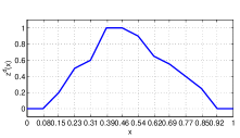
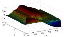
Figure 1: Evolution of heat distribution: (a) desired profile; (b) solution surface.

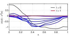
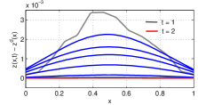
Figure 2: Snapshot of regulation errors: (a) errors for $t\in[0,1]$; (b) errors for $t\in[1,2]$.

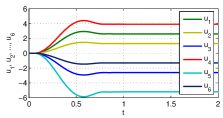
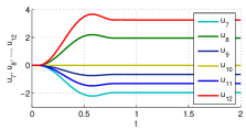
Figure 3: Control signals: (a) $u_{1}$ to $u_{6}$; (b) $u_{7}$ to $u_{12}$.

6 Conclusion

This paper presented a solution to the problem of set-point control of heat distribution with in-domain actuation described by an inhomogeneous parabolic PDE. To apply the paradigm of zero dynamic inverse, the system is presented in an equivalent parallel connection form. The technique of flat systems is employed in the design of dynamic control and motion planning. As the control with multiple in-domain actuators results in a MIMO problem, a Green’s function-based reference trajectory decomposition is introduced, which considerably simplifies the design and the implementation of the developed control scheme. The convergence and solvability analysis confirms the validity of the control algorithm and the simulation results demonstrate the viability of the proposed approach. Finally, as both ZDI design and flatness-based control can be carried out in a systematic manner, we can expect that the approach developed in this work may be applicable to a broad class of distributed parameter systems.

References

References

- [1] A. Bensoussan, G. Da Prato, M. Delfor, S. K. Mitter, Representation and Control of Infinite-Dimensional Systems, 2nd Ed., Birkhäuser, Boston, 2007.
- [2] R. F. Curtain, H. J. Zwart, An Introduction to Infinite-Dimensional Linear System Theory, Vol. 12 of Text in Applied Mathematic, Springer-Verlag, NY, 1995.
- [3] I. Lasiecka, R. Triggiani, Control Theory for Partial Differential Equations: Volume 1, Abstract Parabolic Systems, Cambridge University Press, Cambridge, UK, 2000.
- [4] M. Tucsnak, G. Weiss, Observation and Control for Operator Semigroups, Birkhauser Verlag AG, Basel, 2009.
- [5] M. Krstić, A. Smyshyaev, Boundary Control of PDEs: A Course on Backstepping Designs, SIAM, New York, 2008.
- [6] A. Smyshyaev, M. Krstić, Adaptive Control of Parabolic PDEs, Princeton University Press, Princeton, New Jersey, 2010.
- [7] D. Tsubakino, M. Krstic, S. Hara, Backstepping control for parabolic pdes with in-domain actuation, in: Proc. of the 2012 American Control Conference, Montreal, Canada, 2012, pp. 2226–2231.
- [8] A. Kharitonov, O. Sawodny, Flatness-based feedforward control for parabolic distributed parameter systems with distributed control, Int. J. of Control 79 (7) (2006) 677–687.
- [9] B. Laroche, P. Martin, P. Rouchon, Motion planning for the heat equation, Int. J. of Robust Nonlinear Control 10 (2000) 629–643.
- [10] A. F. Lynch, J. Rudolph, Flatness-based boundary control of a class of quasilinear parabolic distributed parameter systems, Int. J. of Control 75 (15).
- [11] T. Meurer, Control of Higher-Dimensional PDEs: Flatness and Backstepping Designs, Springer, Berlin, 2013.
- [12] N. Petit, P. Rouchon, J. M. Boueih, F. Guerin, P. Pinvidic, Control of an industrial polymerization reactor using flatness, Int. J. of Control 12 (5) (2002) 659–665.
- [13] J. Rudolph, Flatness Based Control of Distributed Parameter Systems, Shaker-Verlag, Aachen, 2003.
- [14] B. Schörkhuber, T. Meurer, A. Jüngel, Flatness of semilinear parabolic PDEs–a generalized Cauchy-Kowalevski approach, IEEE Trans. on Automatic Control 58 (9) (2013) 2277–2291.
- [15] F. Malchow, O. Sawodny, Feedforward control of inhomogeneous linear first order distributed parameter systems, in: Proc. of the 2011 American Control Conference, San Francisco, CA, 2011, pp. 3597–3602.
- [16] T. Meurer, Flatness-based trajectory planning for diffusion-reaction systems in a parallelepipedon - a spectral approach, Automatica 47 (5) (2011) 935–949.
- [17] T. Meurer, A. Kugi, Tracking control for boundary controlled parabolic pdes with varying parameters: Combining backstepping and differential flatness, Automatica 45 (2009) 1182–1194.
- [18] I. Lasiecka, R. Triggiani, Control Theory for Partial Differential Equations: Continuous and Approximation Theories, Cambridge Universioty Press, Cambridge, UK, 2000.
- [19] C. I. Byrnes, D. S. Gilliam, Asymptotic properties of root locus for distributed parameter systems, in: Proc. of the 27th IEEE Conference on Decision and Control, Austin, Texas, 1988, pp. 45–51.
- [20] C. I. Byrnes, D. S. Gilliam, On the transfer function of the zero dynamics for a boundary controlled heat problem in two dimensions, in: Proc. of the 48th IEEE Conference on Decision and Control, Shanghai, China, 2009, pp. 2369–2374.
- [21] C. I. Byrnes, D. S. Gilliam, A. Isidori, V. I. Shubov, Set point boundary control for a nonlinear distributed parameter system, in: Proc. of the 42nd IEEE Conference on Decision and Control, Maui, Hawaii, 2003, pp. 312–317.
- [22] C. I. Byrnes, D. S. Gilliam, A. Isidori, V. I. Shubov, Interior point control of a heat equation using zero dynamics design, in: Proc. of the 2006 American Control Conference, Minneapolis, Minnesota, 2006, pp. 1138–1143.
- [23] C. I. Byrnes, D. S. Gilliam, A. Isidori, V. I. Shubov, Zero dynamics design modeling and boundary feedback design for parabolic systems, Mathematical and Computer Modelling 44 (9-10) (2006) 857–869.
- [24] C. I. Byrnes, D. S. Gilliam, C. Hu, V. I. Shubov, Asymptotic regulation for distributed parameter systems via zero dynamics inverse design, Int. J. of Robust and Nolinear Control 23 (3) (2013) 305–333.
- [25] M. Fliess, J. Lévine, P. Martin, P. Rouchon, Flatness and defect of nonlinear system introductory theory and examples, Int. J. of Control 61 (1995) 1327–1361.
- [26] R. Rebarber, Exponential stability of coupled beam with dissipative joints: A frequency domain approach, SIAM J. Control Opt. 33 (1) (1995) 1–28.
- [27] M. Fliess, P. Martin, N. Petit, P. Rouchon, Active restoration of a signal by precompensation technique, in: the 38th IEEE Conf. on Decision and Control, Phoenix, AZ, 1999, pp. 1007–1011.
- [28] H. Mounier, J. Rudolph, M. Petitot, M. Fliess, A flexible rod as a linear delay system, in: Proc. of the 3rd European Control Conference, Rome, Italy, 1995.
- [29] P. Rouchon, Motion planning, equivalence, and infinite dimensional systems, Int. J. Appl. Math. Comp. Sc. 11 (1) (2001) 165–180.
- [30] W. B. Dunbar, N. Petit, P. Rouchon, P. Martin, Motion planning for a nonlinear stefan problem, ESAIM: Control, Optimisation and Calculus of Variations 9 (2003) 275–296.