Entanglement in a linear coherent feedback chain of nondegenerate optical parametric amplifiers
Abstract
This paper is concerned with linear quantum networks of nondegenerate optical parametric amplifiers (NOPAs), with up to 6, which are interconnected in a coherent feedback chain. Each network connects two communicating parties (Alice and Bob) over two transmission channels. In previous work we have shown that a dual-NOPA coherent feedback network generates better Einstein-Podolsky-Rosen (EPR) entanglement (i.e., more two-mode squeezing) between its two outgoing Gaussian fields than a single NOPA, when the same total pump power is consumed and the systems undergo the same transmission losses over the same distance. This paper aims to analyze stability, EPR entanglement between two outgoing fields of interest, and bipartite entanglement of two-mode Gaussian states of cavity modes of the -NOPA networks under the effect of transmission and amplification losses, as well as time delays. It is numerically shown that, in the absence of losses and delays, the network with more NOPAs in the chain requires less total pump power to generate the same degree of EPR entanglement. Moreover, we report on the internal entanglement synchronization that occurs in the steady state between certain pairs of Gaussian oscillator modes inside the NOPA cavities of the networks.
1 Introduction
Entanglement is a key factor in certain quantum information processing tasks, such as quantum teleportation [1, 2]. Continuous-variable quantum information is highly motivated, as preparation of continuous-variable entangled states is efficient and mathematical description of a continuous variable system is adapted to various physical systems (e.g., quadrature operators of light and total angular momentum operators of an ensemble of atoms satisfy the canonical commutation relations) [3, 4, 5]. In particular, Gaussian states play an important role in continuous-variable quantum information ascribable to 1) physically, the ground state of a quantized electromagnetic field is a Gaussian state; 2) mathematically, though an arbitrary Gaussian state lives in an infinite Hilbert space, it is simply and completely characterized by the mean and (symmetrized) covariance of field operators, which are represented by a vector and a matrix with finite dimensions, respectively; 3) experimentally, entanglement in Gaussian states is easily obtained [5, 6, 7, 8]. For instance, Gaussian entangled beams can be generated by employing a strong coherent pump beam to shine a nonlinear crystal inside the cavity of a nondegenerate optical parametric amplifier (NOPA). Interactions between the pump beam and two modes in the cavity produce a pair of entangled outgoing fields in Gaussian states which have strong correlations in quadrature-phase amplitudes [8]. Such entanglement is called Einstein-Podolsky-Rosen (EPR) entanglement.
In this paper, we investigate EPR entanglement between two propagating continuous-mode light fields and bipartite entanglement of two-mode Gaussian states. The former one, namely, the two-mode squeezing of the two continuous-mode fields, is characterized by a two-mode squeezing spectrum , which can be obtained via an associated quantum Langevin equation. Strong EPR entanglement is indicated by a high degree of two-mode squeezing over a wide frequency range. The sufficient condition of EPR entanglement existing at a certain frequency for a pair of quadrature-phase amplitudes is that the value of the corresponding satisfies a sum criterion [8, 9]. On the other hand, entanglement of two-mode Gaussian states can be measured by the logarithmic negativity in the time domain. The logarithmic negativity is calculated based on the covariance matrix of the position and momentum operators corresponding to the two modes. For strong entanglement, has a high positive value [7, 10]. More details of the two quantities of entanglement are given in Section 4.
In reality, a quantum system is dissipative due to interactions between the system and its environment. Such inevitable losses degrade entanglement. Thus, transmission distance and communication quality are limited. Failure of the communication may even happen [1, 11]. Consequently, reliable generation and distribution of entanglement in the presence of losses in transmission channels is a central issue in quantum communications.
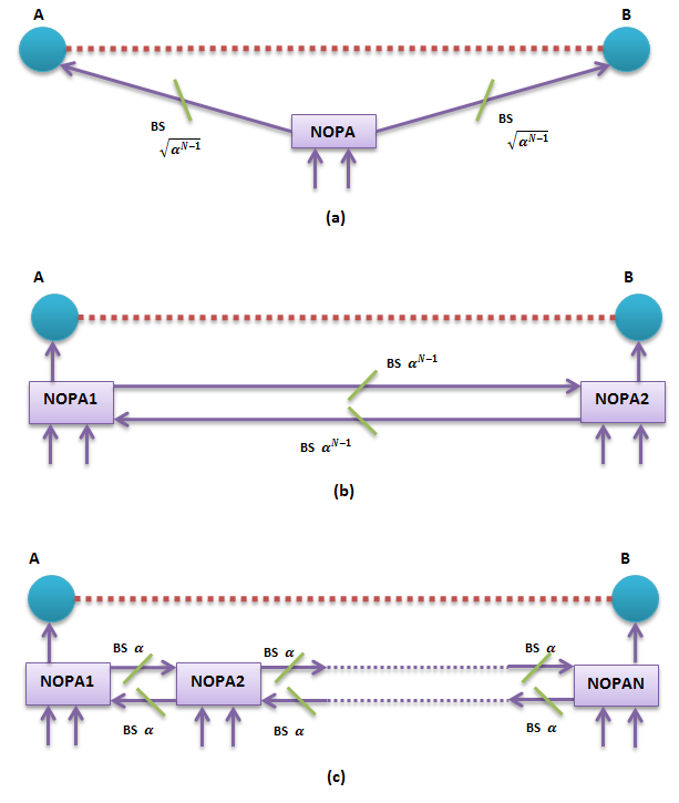
Our previous work [12] has investigated EPR entanglement prepared by a dual-NOPA coherent feedback network where the two NOPAs are distributed separately at two distant communicating ends (Alice and Bob), as shown in Fig. 1 (b). The degree of EPR entanglement is influenced by the total pump power applied to the system, values of the damping rates of the NOPAs, amplification losses induced by unwanted interactions between a NOPA and its environment, as well as transmission losses caused by leakage of photons along the transmission channels. Moreover, time delays in the process of transmission narrow the bandwidth of suppressed two-mode squeezing. Compared to a single NOPA placed in between the two ends (at Charlie’s) over the same transmission distance as indicated in Fig. 1 (a), the coherent feedback configuration consumes less total pump power to achieve the same degree of EPR entanglement when amplification losses are ignored and the damping rates of the systems are identical; on the other hand, the dual-NOPA system proposed in [12] achieves higher level of EPR entanglement against transmission losses under the same total pump power and damping rates. More precisely, for sufficiently high transmission rates one would employ a distributed version of the scheme, while for low transmission rates a centralised architecture would be employed to give enhanced entanglement under the same pump power and damping rates.
This paper studies a coherent feedback configuration of up to six NOPAs that are evenly deployed between two ends (Alice and Bob) and connected in a linear coherent feedback interconnection, as shown in Fig. 1 (c). Descriptions of optical components employed in the system as well as the dynamics of the system under the effects of losses and time delays are given in Section 2. Section 3 gives an analysis of stability conditions in systems without and with losses. We prove a theorem showing that the stability thresholds can be obtained by solving certain polynomials. Section 4 is devoted to investigating and comparing degrees of end-to-end EPR entanglement of the -NOPA systems in absence of time delays but with losses considered. We give the ideal values of and as shown in Fig 2 for -NOPA systems with the even number and the odd number of NOPAs. Moreover, we look into entanglement of two-mode Gaussian states related to pairs of optical cavity modes. In this section, there are some qualitative findings such as in the absence of losses, the degree of end-to-end entanglement increases as the amplitude of pump beam for each NOPA approaches the value at which the system just loses stability; in the presence of losses, there exists an optimal value of pump amplitude of NOPAs for the end-to-end entanglement; the entanglement generated between collective modes is different between systems with an even and odd number of NOPAs; with the same pump power and without losses, increasing the number of NOPAs improves the end-to-end entanglement but not the entanglement of internal two-mode Gaussian states. The interesting qualitative observations described above are not straightforward to analyze quantitatively, so their quantitative analyses are left as topics for future research. Section 5 explores effects of time delays on the stability and entanglement of the systems. Finally, we restate the main results of this paper as a conclusion in Section 6.
The following notations are adopted in this paper: denotes , the transpose of a matrix of numbers or operators is denoted by , and denotes (i) the complex conjugate of a number, (ii) the conjugate transpose of a matrix, as well as (iii) the adjoint of an operator. denotes an by identity matrix, is an by zero matrix (we simply write , if ), trace operator is represented by , denotes the Kronecker delta and denotes the Dirac delta function. denotes quantum expectation and denotes the largest singular value of a matrix.
2 System Model
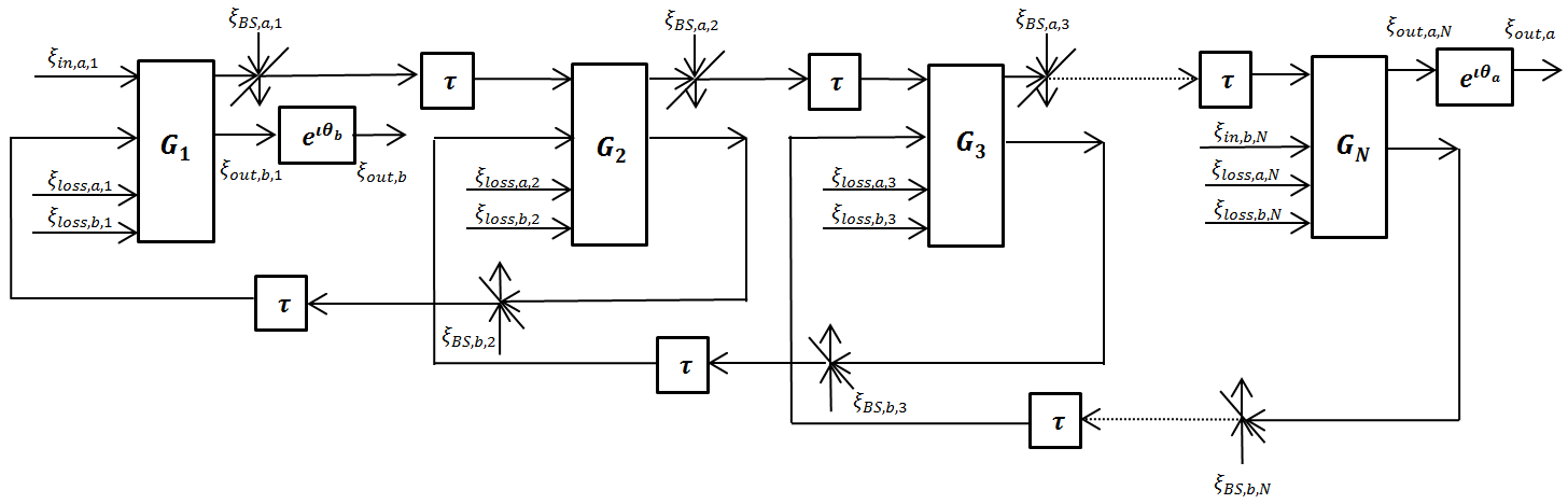
In this section, a brief introduction of quantum optical devices and dynamics of the system is given. Fig. 2 shows a detailed system model of our -NOPA coherent feedback network. We take account of the system undergoing losses and time delays. The first NOPA () and the -th NOPA () are placed at Alice’s and Bob’s, respectively; the other NOPAs are deployed in a linear line in between Alice and Bob. The length of the path between every two neighbouring NOPAs is identical. Transmission losses are modelled by beamsplitters. The time delay in each path is denoted by a constant . Two adjustable phase shifters with phase shifts and , respectively, are placed at two outputs separately in order to obtain the best two-mode squeezing between fields and .
2.1 Quantum optical components
2.1.1 NOPA
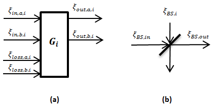
Fig. 3 (a) gives a block diagram representation of a NOPA . Four ingoing boson fields are in the vacuum state, among which and are unwanted amplification losses. The field operators comply with the commutation relations, that is, for a boson field operator , we have . The main component of NOPA is a two-ended cavity with two orthogonally polarized boson modes and , which obey the commutation relations , , and . The fields , , and interact with the modes via coupling operators , , and , respectively, where and are damping rates. To yield EPR entanglement between outgoing Gaussian fields and , a strong pump beam in a coherent state is employed to shine the nonlinear crystal inside the cavity. The modes are coupled with the beam via the system Hamiltonian , where is a real parameter related to the effective amplitude of the pumping field [8, 13].
The time-varying interaction Hamiltonian between the system and its environment is , where and [14]. The time evolution of the mode and field operators in the Heisenberg picture are given by [13]
where is a unitary process satisfying the quantum white noise equation . Using the rules of quantum stochastic calculus, the dynamics of the NOPA is described by the quantum Langevin equations [8, 13, 15, 16]
| (1) |
and the output fields are
| (2) |
2.1.2 Beamsplitter
The transmission loss in a path between two adjacent NOPAs is caused by loss of photons. It is modelled by a beamsplitter with transmission rate and reflection rate [13, 17]. As shown in Fig. 3 (b), output signal of the beamsplitter is the combination of the two ingoing fields, that is, . In our case, is a white-noise field operator in the ground state and is an outgoing Gaussian field of a NOPA.
Assume the total transmission distance between Alice and Bob is kilometres. Therefore, the length of each path between every two adjacent NOPAs is km. Based on the assumption of that there exists around dB per kilometre transmission loss in optical fibre [18], we obtain that the transmission rate of each beamsplitter is .
2.2 The -NOPA coherent feedback network
Based on the dynamics of a NOPA and the transformation of a beamsplitter as given above, an -NOPA coherent feedback system undergoing transmission losses and time delays as depicted in Fig. 2 has the following dynamics at time , when all the nodes of the network are connected,
| (3) | |||||
with outputs
| (4) | |||||
where and .
As a linear stochastic model, the dynamics of the system can be described by a linear quantum stochastic differential equation in the quadrature operators of the system [19, 20]. Note that quadratures of a bosonic mode, say , are and . Similarly, the quadratures of a field operator, say , are and . Define the vectors of quadratures corresponding to the -NOPA system as
| (5) |
In the absence of time delays, the system dynamics is of the form
| (6) | |||||
| (7) |
For the -NOPA system, the covariance matrix of its -mode Gaussian state is
| (8) |
where is the initial density operator of the system. Furthermore, when time delays are neglected, satisfies the Lyapunov matrix differential equation
| (9) |
Specially, the steady-state covariance matrix satisfies the Lyapunov equation [11, 23]
| (10) |
Define the parameters of the system as follows. For each NOPA, we set Hz and Hz, where () and () are real parameters, and Hz is a reference value for the transmissivity mirrors of the NOPA. Following [12, 21], we assume that when and the value of is proportional to the absolute value of , so we set [12, 21]. Suppose that the total transmission distance is km, then the transmission rate of each beamsplitter is and time delay in the path between any two adjacent NOPAs is around . The range of the adjustable phase shifts and is .
3 Stability analysis
This section is devoted to the stability analysis of our -NOPA system. If the system is unstable, the mean total photon number in the cavity modes is continuously growing, which is undesirable. By stability, we mean that the mean of the quadrature vector becomes a zero vector as time approaches infinity, namely, , and Eq. (10) has a unique solution [24]. The system is stable when in Eq. (6) is Hurwitz, that is, all the eigenvalues of have real negative parts. We are interested in the range of over which stability is assured. However, unlike the dual-NOPA system studied in our previous work [12], it is infeasible to obtain an explicit expression for the stability threshold at which the system just loses stability by checking the Hurwitz property of . Here, by regarding as an uncertainty, we employ the -analysis method from control theory [22] to obtain the following lemma.
Lemma 1
In the absence of time delays, an -NOPA coherent feedback system is stable if and only if and , where .
Proof. First, for convenience, let us define the following matrices,
| (15) | |||
| (24) |
Recall that , then from Eq. (3) and Eq. (6) the matrix of an -NOPA system is a real matrix given by
| (30) |
where . To proceed, we now investigate the robust stability condition of a certain feedback system, as shown in Fig.4. The state space of the system is given by
| (31) |
where and is the state vector. Hence, the transfer function of the system is . As long as the stability condition of this system holds, our -NOPA coherent feedback system is stable.
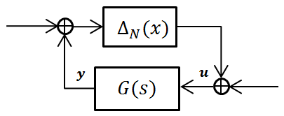
According to Theorem 11.8 in [22], if the system (31) with transfer function is stable, then the closed-loop system in Fig. 4 with structured uncertainty satisfying () is internally stable if and only if
| (32) |
where
| (35) | |||
| (36) |
First, we check the stability of the system (31). Using (24) and (30), we obtain that . Hence is stable because has all its zeros in the left half plane by virtue of the fact that and . Noting that , we have , therefore, . Since , for (32) to be fulfilled we must have that . Since and , we obtain Lemma 1.
Lemma 1 shows that the system is stable as long as does not have any purely imaginary eigenvalues. In fact, we shall prove that has no eigenvalues on the imaginary axis, which leads to the following theorem.
Theorem 2
In the absence of time delays, an -NOPA coherent feedback system is stable if and only if , where is the smallest positive root of the polynomial .
Proof. For convenience, we define , and an invertible matrix
| (45) |
Exploiting (30), the characteristic polynomial of is
| (50) | |||||
where and are matrices given by
| (56) | |||||
| (62) |
Since for any square matrices such that and is invertible, we obtain
| (63) |
and is a symmetric matrix given by
| (70) | |||||
where . Let us define the column of (LABEL:eq:AuAl_n2I) as . Let for any non-zero and apply the following elementary column operations: and for . Thus, the matrix (LABEL:eq:AuAl_n2I) is reduced to a matrix given by
| (78) |
where and is a complex number. As and is a negative real number, it can be found that the columns of the matrix are linearly independent, that is, for a vector , the equality
| (83) |
is true if and only if . Thus, the matrix has full rank, which leads to when . Consequently, non-zero . Following Lemma 1, we obtain the theorem.
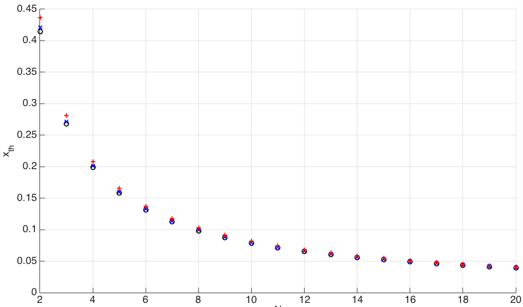
In the rest of paper, we shall numerically analyze stability and entanglement performance of the -NOPA coherent feedback system. To this end, we now set , that is, . Based on Theorem 2, with the help of Mathematica, we get Fig. 5 that plots the values of the stability threshold of our -NOPA systems () in the absence of losses (black circles), with transmission losses only (blue crosses) and with both transmission and amplification losses (red plus signs). The values of of the -NOPA systems () are listed in Table 1. It is indicated that the value of the stability threshold decreases as more NOPAs are added to the network. The rate of decrease becomes smaller as the number of NOPAs grows. Moreover, existence of amplification and transmission losses broadens the range of over which stability is guaranteed. Notice from the figure that the effect of transmission and amplification losses on diminishes for higher values of .
| N | |||
|---|---|---|---|
| () | () | () | |
| 2 | 0.4142 | 0.4209 | 0.4363 |
| 3 | 0.2679 | 0.2715 | 0.2808 |
| 4 | 0.1989 | 0.2013 | 0.2080 |
| 5 | 0.1583 | 0.1602 | 0.1655 |
| 6 | 0.1316 | 0.1331 | 0.1375 |
Note that when values of all system parameters except for are given, we can also use the mussv function in the Robust Control Toolbox of MATLAB to estimate the stability threshold. Details are given in Appendix 1.
4 Entanglement
In this section, entanglement performances are compared among the systems with number of NOPAs varying from 2 to 6, in the absence of time delays. First, we study the EPR entanglement, namely, the two-mode squeezing, between the two outgoing fields when systems are in an ideal case where no losses are present. After that, the effect of transmission and amplification losses on the two-mode squeezing is taken into account. In the end, we analyze the entanglement between pairs of optical cavity modes in the system using logarithmic negativity as an entanglement measure.
4.1 End-to-end EPR entanglement
Strong correlation between quadrature-phase amplitudes of two fields is a manifestation of EPR entanglement [8]. The EPR entanglement between two continuous-mode fields is quantified in frequency domain. To this end, we define the Fourier transforms of and in Eq. (4) as and . The two-mode amplitude spectrum and the two-mode phase spectrum are defined as [8]
Furthermore, based on (3) and (4), the two-mode squeezing spectra are obtained by [25, 26]
| (84) | |||||
| (85) |
where , , and is the transfer function of the -NOPA system. Note that for all .
Define the two-mode squeezing spectrum as
| (86) |
The fields and in the system shown in Fig. 2 are EPR entangled at the frequency rad/s if such that satisfies the sum criterion [9],
| (87) |
Perfect two-mode squeezing has the feature that [8]. Of course, perfect squeezing cannot be achieved in practice. Therefore, one aims instead to have a small value over a wide frequency range [9]. According to [12, 25], holds at low frequencies. Thanks to this, we can simply focus on the two-mode spectra and at for the rest of the paper.
In this paper, plots of the two-mode spectra are presented in dB unit, that is, and . In this case, perfect EPR entanglement at frequency corresponds to . Better two-mode squeezing is indicated by a more negative value of .
4.1.1 An ideal case.
Now we examine the two-mode spectra when the -NOPA system is lossless. First, we aim to find values of and at which the cost function at is minimized. Based on (84), (85) and via Mathematica, we obtain Table LABEL:tb:Vthetas which presents the formulas of the two-mode squeezing spectra of -NOPA systems in the ideal case.
| N | |
|---|---|
For any value of in the interval , we have for the -NOPA system, for the -NOPA system, for the -NOPA system, for the -NOPA system, and for the -NOPA system. Recall that the values of the stability threshold are listed in Table 1. Thus, for systems with an even number of NOPAs, the best two-mode squeezing is obtained if or ; for systems with an odd number of NOPAs, the best two-mode squeezing is achieved when . In this regard, we set
| (90) |
In the rest of paper, and are defined as the two-mode spectra at the fixed values of and as given in (90).
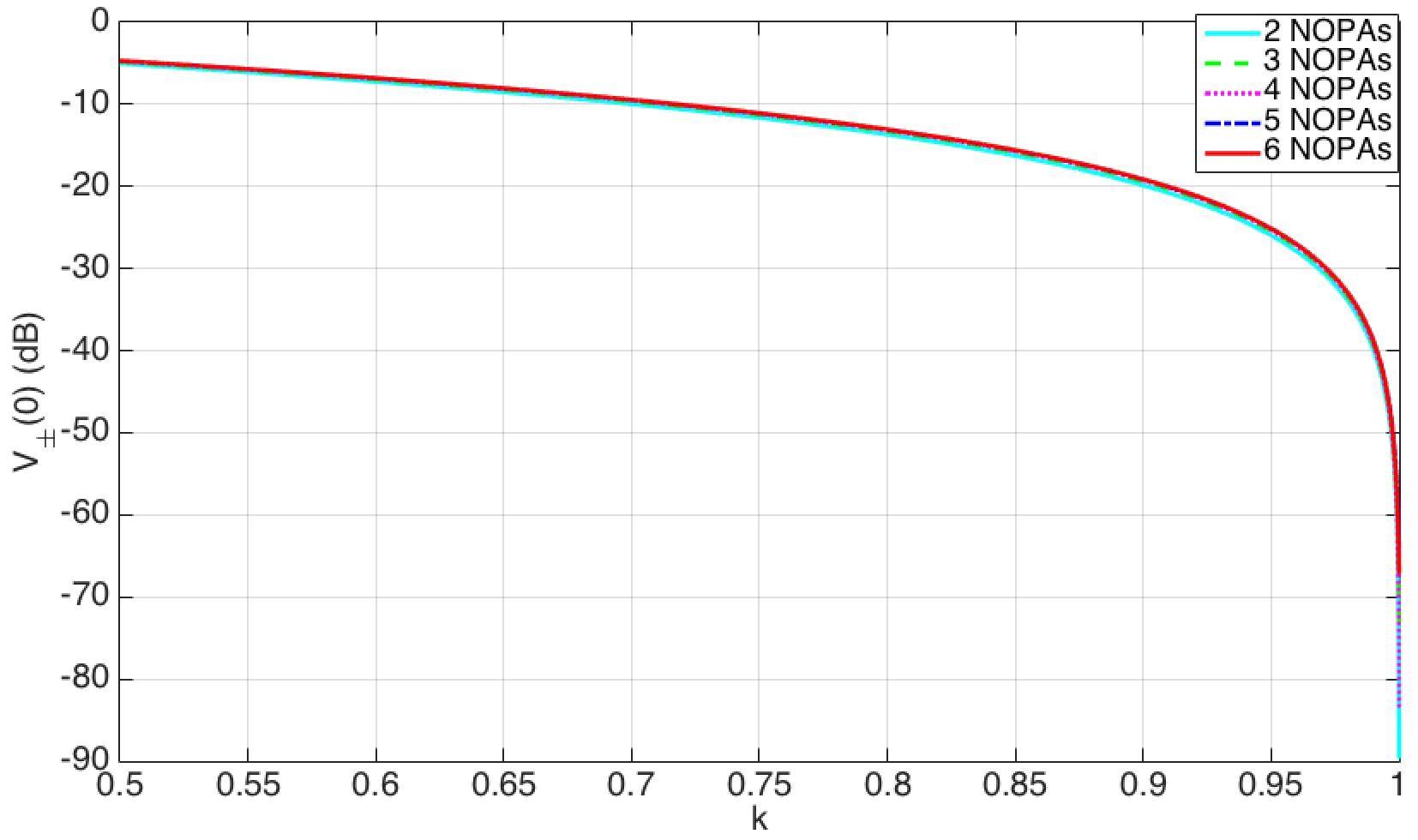
Now we check the two-mode spectra as a function of at , where as the value of varies from to . As shown in Fig. 6, the two-mode squeezing spectra decrease as the value of approaches the stability threshold. Moreover, the rates of the decreases are similar.
One of our interests is the power consumption of the systems to generate the same level of EPR entanglement, say, . We denote the corresponding as . Here the power of pump beam employed by each NOPA is . Hence, the total pump power of an -NOPA system is . Since is a fixed reference, to compare pump consumption between different values of , it is enough to consider only the quantity . As the third column of Table 3 indicates, a system with more NOPAs consumes less power to yield the same degree of two-mode squeezing.
4.1.2 Effects of losses.
The effect of losses on the two-mode squeezing of the systems is indicated in Table 3. All the systems have the same value of () when losses are neglected. EPR entanglement of each system is degraded by around under the effect of transmission losses, and the reduction is more than if both transmission and amplification losses are present. Generally, a system employing more NOPAs provides a slight improvement in EPR entanglement when transmission losses are present, in the absence of amplification losses. This merit disappears in the presence of both transmission and amplification losses. In this case, the system with more NOPAs yields less EPR entanglement.
| N | ||||||
|---|---|---|---|---|---|---|
| (, | (, | (, | (, | ( | ||
| ) | ) | ) | ) | ) | ||
| 2 | 0.3978 | 0.3165 | -13.3150 | -10.3047 | -7.5838 | -4.5735 |
| 3 | 0.2579 | 0.1995 | -13.3286 | -10.3183 | -7.4114 | -4.4011 |
| 4 | 0.1916 | 0.1468 | -13.3302 | -10.3199 | -7.3510 | -4.3407 |
| 5 | 0.1526 | 0.1164 | -13.3295 | -10.3192 | -7.3236 | -4.3133 |
| 6 | 0.1269 | 0.0966 | -13.3306 | -10.3203 | -7.3078 | -4.2975 |
| N | ||||
|---|---|---|---|---|
| 2 | 0.4074 | 0.3319 | -13.3683 | -10.3580 |
| 3 | 0.2644 | 0.2097 | -13.3928 | -10.3825 |
| 4 | 0.1965 | 0.1544 | -13.3991 | -10.3888 |
| 5 | 0.1565 | 0.1225 | -13.4018 | -10.3915 |
| 6 | 0.1302 | 0.1017 | -13.4033 | -10.3930 |
| N | ||||
|---|---|---|---|---|
| 2 | 0.3770 | 0.2843 | -7.6545 | -4.6442 |
| 3 | 0.2435 | 0.1779 | -7.4982 | -4.4879 |
| 4 | 0.1805 | 0.1303 | -7.4435 | -4.4332 |
| 5 | 0.1438 | 0.1034 | -7.4182 | -4.4079 |
| 6 | 0.1195 | 0.0857 | -7.4044 | -4.3941 |
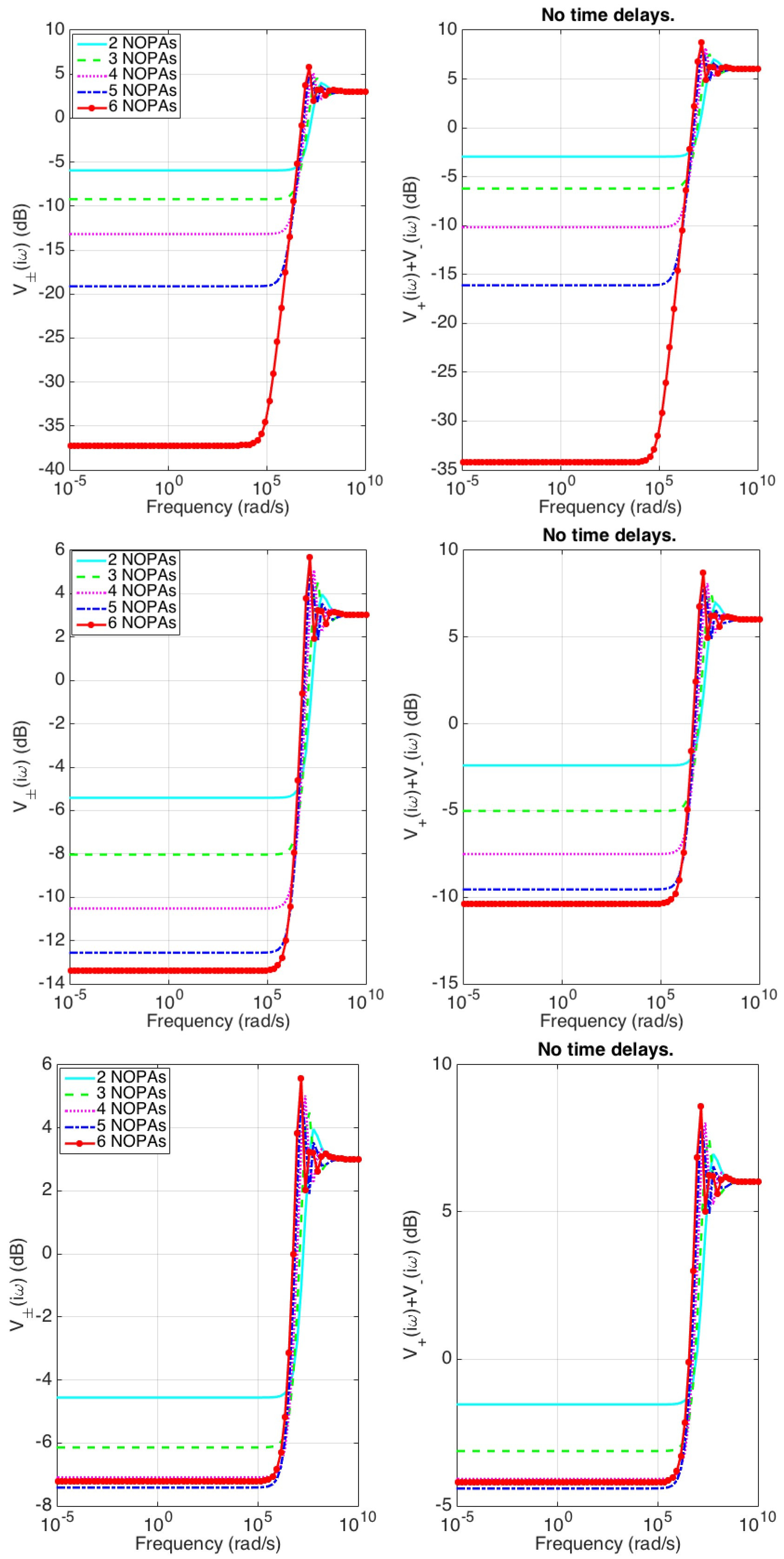
Now we compare the two-mode squeezing levels when the systems are consuming the same total pump power. From now on, we use to denote of the system with NOPAs. In this case, we set , hence (). The two-mode squeezing spectra in the (ideal) lossless case, in the presence of transmission losses only, as well as under effect of both transmission and amplification losses are plotted in Fig. 7. With the same total power, a system consisting of more NOPAs yields stronger EPR entanglement, except that when both transmission and amplification losses are present, the 6-NOPA system has a slightly lower degree of EPR entanglement than the 5-NOPA one. Moreover, the EPR entanglement of the system with less NOPAs has smaller change under the influence of losses.
To find the approximate value of at which the system achieves the highest degree of two-mode squeezing at under the effect of losses, we pick the smallest one among the values of corresponding to a thousand samples of evenly spread through the range . Tables 4 and 5 illustrate the values of , the corresponding two-mode squeezing degrees, and the total power consumptions of the -NOPA systems in the scenarios with only transmission losses as well as when both transmission and amplification losses are present, respectively. As the tables indicate, the best two-mode squeezing degrees of all the systems are similar, however, the system with more NOPAs consumes less total pump power. For instance, a 6-NOPA system needs less than a third of power used by the dual-NOPA system. Thus, the system should employ more NOPAs in the presence of losses for efficient use of pump power, while only losing a small amount of EPR entanglement.
4.2 Entanglement of two-mode Gaussian states
In this sub-section, we study the entanglement of two-mode Gaussian states with respect to the cavity mode operators when the -NOPA system is lossless. To this end, we first calculate the covariance matrix and steady-state covariance matrix of the -mode Gaussian state of the system. Based on Eq. (8), (9) and (10), we employ the Matlab functions with the sampling time and to compute and , respectively. Here, we take corresponding to that the system starts in a vacuum state.
The covariance matrix of the modes and () is a corresponding sub-matrix of . For instance, the covariance matrix of and in a -NOPA system is
| (95) |
Entanglement of two-mode Gaussian states with corresponding covariance matrix is measured by the logarithmic negativity [10, 23]. Write in a block matrix form given by
| (98) |
where is a matrix. Define
| (99) | |||
| (100) |
Then is a nonnegative real number given by
| (101) |
represents that the modes and are separable at time , that is, there is no entanglement between the modes. Strong entanglement between modes and is represented by a high value of .
What is of interest to us are the time evolution and steady-state values of logarithmic negativities , , , as well as of an -NOPA () coherent feedback network. Besides, the logarithmic negativity of and is also looked into. The reason is that, as (2) indicates, when losses and delays are neglected, the outputs and contain and , respectively. Notice that and can be viewed as collective single mode annihilation operators as they satisfy the commutation relations , , and . The covariance matrix of and is , with .
| N | |||||||
| 2 | 0 | 0 | 0.4850 | 0.1921 | 0.1921 | ||
| N | |||||||
| 3 | 0.0561 | 0 | 0 | 0.2865 | |||
| 0.3645 | 0.3645 | 0 | |||||
| 0.1144 | 0.1144 | 0.1144 | |||||
| N | |||||||
| 4 | 0 | 0 | 0 | 0 | 0.1843 | ||
| 0.2803 | 0.3021 | 0.2803 | 0 | ||||
| 0.0722 | 0.0722 | 0.0722 | 0.0722 | ||||
| N | |||||||
| 5 | 0.0223 | 0 | 0 | 0 | 0 | 0.1207 | |
| 0.2134 | 0.2500 | 0.2500 | 0.2134 | 0 | |||
| 0.0451 | 0.0451 | 0.0451 | 0.0451 | 0.0451 | |||
| N | |||||||
| 6 | 0 | 0 | 0 | 0 | 0 | 0 | 0.0767 |
| 0.1552 | 0.2033 | 0.2195 | 0.2033 | 0.1552 | 0 | ||
| 0.0260 | 0.0260 | 0.0260 | 0.0260 | 0.0260 | 0.0260 |
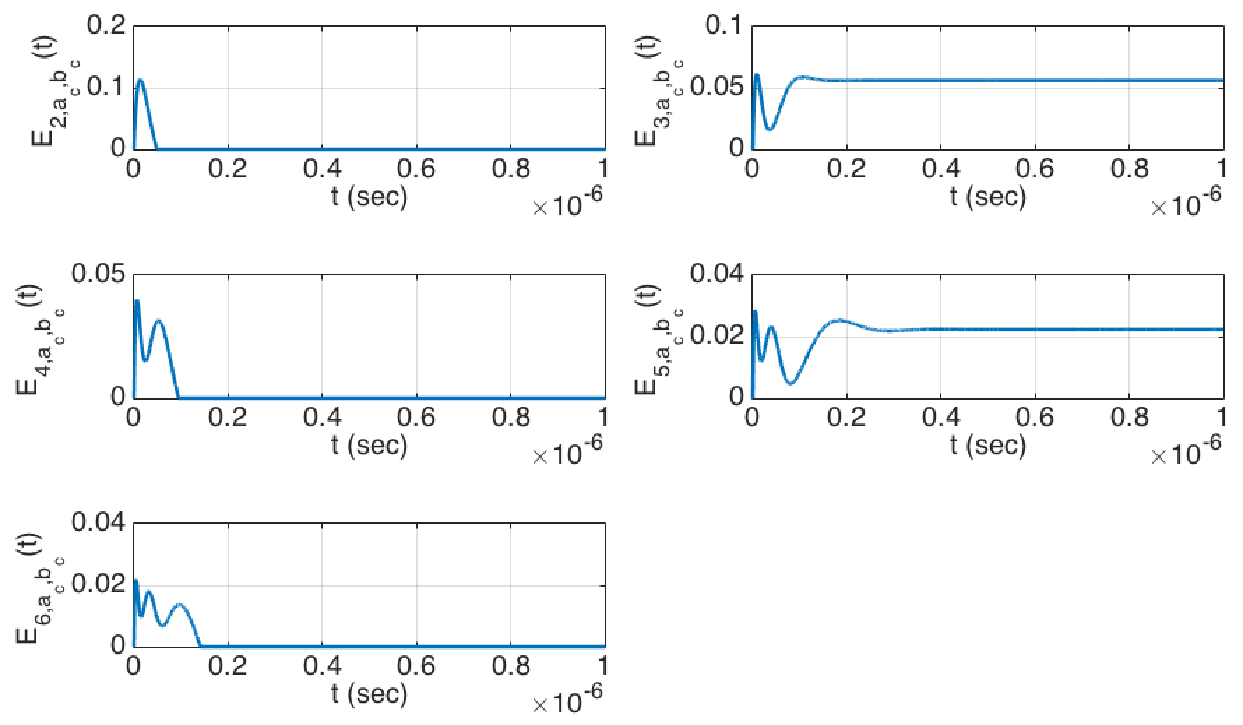
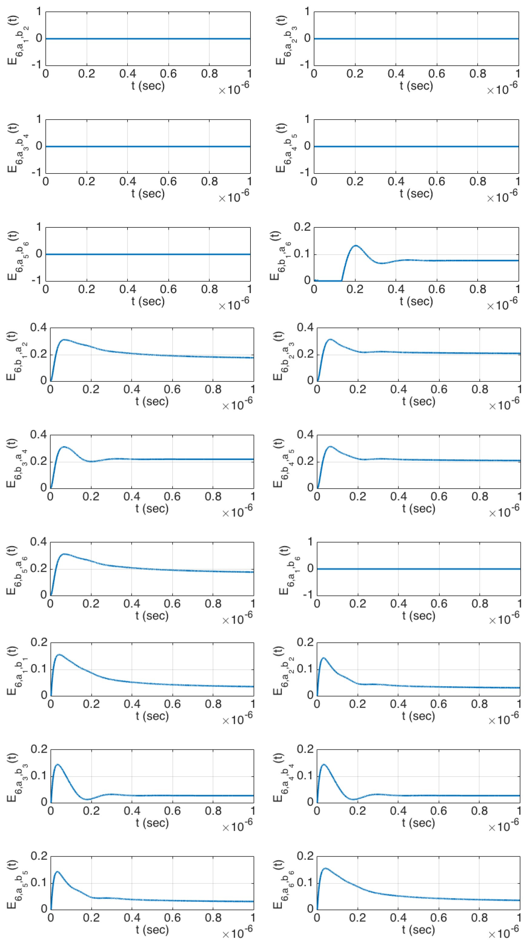
In the absence of losses and delays, Table 6 shows the values of steady-state logarithmic negativities of the -NOPA systems, Fig. 8 indicates the time evolution of , and Fig. 9 plots the evolution of logarithmic negativities of a -NOPA coherent feedback network. As indicated, and remain separable for all time, and the same happens to and . At steady state, entanglement exists between modes and , and , as well as and . In particular, it can be observed that internal entanglement synchronization occurs at steady state, that is, the degree of entanglement between the oscillator modes and in the cavity of each NOPA in the -NOPA coherent feedback network is the same. For systems with an odd number of NOPAs, there is slight entanglement between the collective modes and , while in systems containing an even number of NOPAs, and are entangled at the beginning for a very short time. After that, the entanglement rapidly vanishes. Moreover, with the same total pump power, entanglement of two-mode Gaussian states in the system with more NOPAs is weaker. It is an interesting result that even though the two-mode entanglement of the internal cavity modes does not improve for systems carrying more NOPAs, its EPR entanglement between the two outgoing fields does improve.
5 Effect of Time Delays
In this section, we investigate stability and entanglement of the -NOPA systems in the presence of losses and time delays. For a km transmission distance, the time delay of each path between two neighbouring NOPAs is . To check stability of our time-delayed -NOPA systems, we employ the DDE-BIFTOOL toolbox [27, 28], which is a Matlab package used to plot the eigenvalues of a linear delay differential system. A system is stable if all real parts of the eigenvalues are negative. Based on the above fact, we find that stability of the -NOPA systems for up to six is guaranteed in the case where the systems are given the same total pump power, and both losses and delays are present.
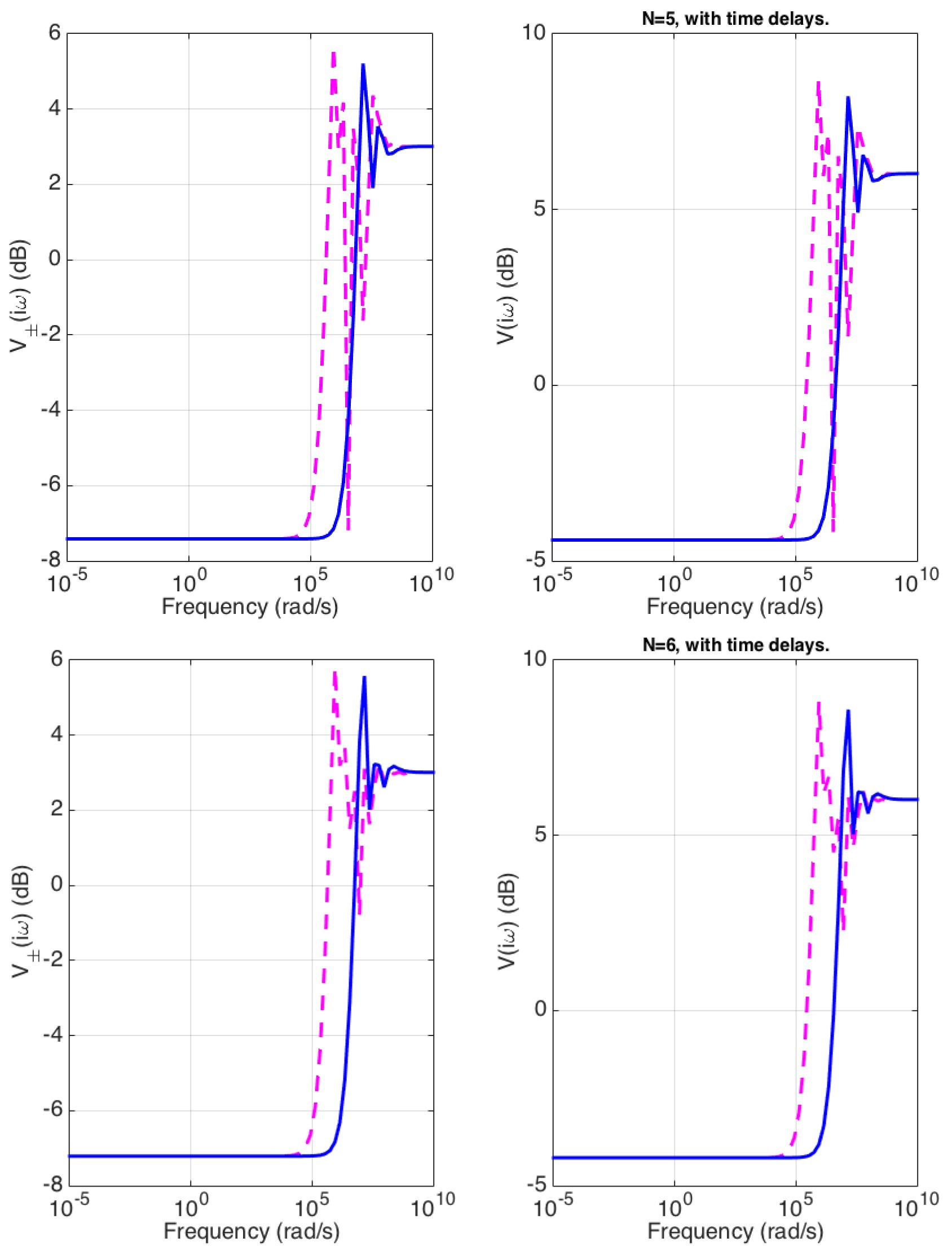
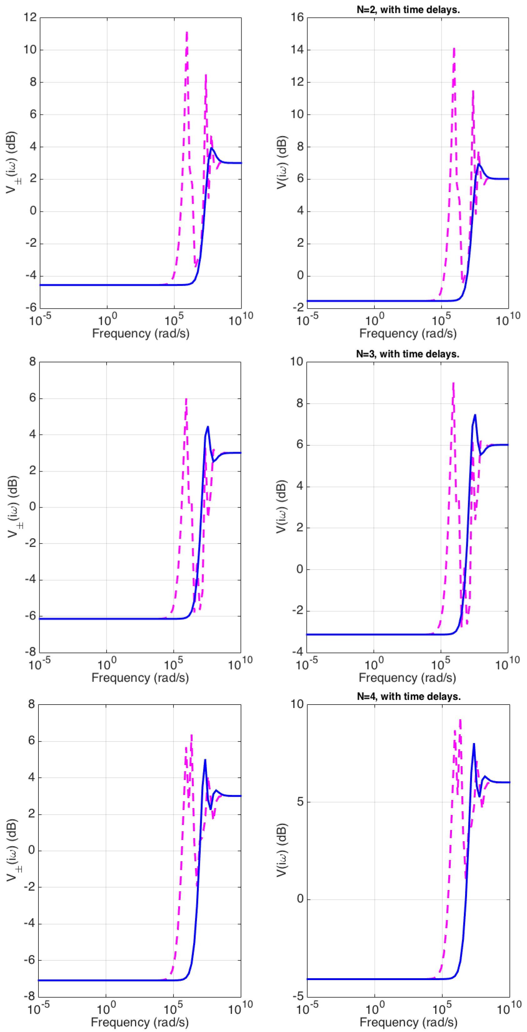
As a linear quantum system, the -NOPA network with time delays can be built in Matlab via commands connect and delayss in the Matlab Control System Toolbox. The non-rational transfer functions (due to the time delays) and in (84) and (85) can be numerically computed with the built-in Matlab frequency response command freqresp. Therefore, the two mode squeezing spectra are obtained via (84) and (85). The effect of time delays on EPR entanglement between the outgoing fields of our -NOPA system is indicated in Fig. 10 and Fig. 11, where all the systems are given the same total pump power and undergoing both transmission and amplification losses. Compared with the two-mode squeezing of the systems in the absence of delays, the presence of time delays reduces the bandwidth over which the EPR entanglement exists, but does not impact the EPR entanglement degrees at low frequencies. The phenomenon of the sharp peaks and dips at high frequencies is a common feature of the frequency response of systems under the effect of internal time delays, see, e.g, [29, p. 182]. In our case, the bandwidth of EPR entanglement under influence of time delays is similar for all the systems with a different .
6 Conclusion
This paper has studied the stability condition and entanglement performance of an -NOPA coherent feedback network with up to six, where the NOPAs are evenly distributed in a line between two distant parties, Alice and Bob. The system undergoes transmission losses, amplification losses and time delays. Moreover, two adjustable phase shifts and are placed at Alice and Bob for achieving the best two-mode squeezing between the two outgoing fields by selecting appropriate quadratures of the output fields.
In the absence of time delays, we have derived a necessary and sufficient stability condition with the aid of -analysis method from control theory [22] by regarding , the parameter related to the amplitude of pump beam, as an uncertainty. We have shown that, the value of stability threshold is the smallest positive root of the polynomial . It is observed that the existence of losses broadens the range of over which stability is guaranteed, and the value of decreases as more NOPAs are added to the system.
Strong EPR entanglement is represented by strong attenuation of two-mode output squeezing spectra below the sum criterion. In the ideal case, we have found the values of and at which the system achieves the best two-mode squeezing. Moreover, the two-mode squeezing increases rapidly as the value of approaches the stability threshold .
We have compared the two-mode squeezing generated by systems with different numbers of NOPAs. It is shown that, to achieve the same squeezing level in the ideal case, the system employing more NOPAs requires less total pump power. When losses are present, all the systems have a large and similar decrease in EPR entanglement. Given the same total pump power, the system carrying more NOPAs has improvement in the two-mode squeezing in the ideal case and when only transmission losses are present. However, this is no longer assured when amplification losses are also taken into account. Furthermore, the best two-mode squeezing degrees of the systems with losses are similar. However, the system with more NOPAs requires less pump power to achieve the best two-mode squeezing.
We have also investigated the entanglement of two-mode Gaussian states of the internal cavity modes. Steady-state values and time evolution of logarithmic negativities have been studied. It is shown that entanglement exists between the modes and , and as well as and . Moreover, we have observed an internal entanglement synchronization that occurs between the modes and for at steady state. In the ideal case, given the same pump power, though the system with more NOPAs has improved two-mode squeezing in the output fields, it does not have better internal entanglement between cavity modes as measured by logarithmic negativity.
Stability and entanglement under the effect of time delays has been studied as well. With time delays, stability is checked with the DDE-BIFTOOL toolbox [27, 28]. It is shown that, with transmission and amplification losses, time delays narrow the bandwidth over which the EPR entanglement exists.
This work gives several qualitative findings on entanglement in the -NOPA network when , which have not been quantitatively analyzed and are topics suitable for future investigations. It is observed that the two-mode squeezing spectra decreases as the value of approaches when the system is lossless, and there exists an optimal value of for the two-mode squeezing when the system is under losses. These phenomena are not surprising and to some extent predictable as they were proved for the -NOPA system in our previous work, see Theorem 2 and Theorem 3 in [12]. In addition, future work is still required to quantitatively analyze the observation that entanglement between collective modes behaves differently between systems with an even and the odd number of NOPAs; also, adding more NOPAs into the system improves the end-to-end entanglement between continuous-mode output fields but not the entanglement of internal two-mode Gaussian states when the system is lossless and consumes the same pump power. Moreover, it would be of interest to quantitatively analyze the behaviour of the linear coherent feedback chain in the asymptotic limit of .
Appendix 1
When values of all parameters except for of an -NOPA coherent feedback system are given, we can employ the mussv function in the Robust Control Toolbox of MATLAB to approximate the stability threshold. The approximated stability threshold, say , approaches the stability threshold from the left. That is, the system is robustly stable when the value of belongs to the range and approximates the threshold value . The value of is found by the following bisection algorithm.
Step 1. Start from . If the system is not stable over the range , set and ; otherwise stop.
Step 2. Set . If the system is not stable over the range , set ; otherwise set .
Step 3. If the value of for a prespecified error tolerance (here, we take ), go back to Step 2; otherwise set , stop.
References
- [1] M. A. Nielsen and I. L. Chuang (2000), Quantum computation and quantum information, Cambridge University Press.
- [2] W. P. Bowen, R. Schnabel, P. K. Lam and T. C. Ralph (2004), A characterization of continuous variable entanglement, Phys. Rev. A, 69, pp. 012304.
- [3] S. L. Braunstein and P. Loock (2005), Quantum information with continuous variables, Rev. Mod. Phys, 77, pp. 513-577.
- [4] C. Weedbrook, S. Pirandola, R. Garcia-Patron, N. J. Cerf, T. C. Ralph, J. H. Shapiro and S. Lloyd 2012, Gaussian quantum information, Rev. Mod. Phys. 84, pp. 621.
- [5] G. Adesso, S. Ragy and A. R. Lee (2014), Continuous variable quantum information Gaussian states and beyond, Open Systems & Information Dynamics, 21, pp. 1440001.
- [6] A. Ferraro, S. Olivares and M. G. A. Paris (2005), Gaussian states in continuous variable quantum information, Napoli Series on Physics and Astrophysics (ed. Bibliopolis, Napoli).
- [7] G. Adesso and F. Illuminati (2007), Entanglement in continuous-variable systems: recent advances and current perspectives, J. Phys. A: Math. Theor, 40, pp. 7821–7880.
- [8] Z. Y. Ou, S. F. Pereira and H. J. Kimble (1992), Realization of the Einstein-Podolsky-Rosen paradox for continuous variables in nondegenerate parametric amplification, Appl. Phys. B, 55, pp. 265.
- [9] D. Vitali, G. Morigi, and J. Eschner (2006), Single cold atom as efficient stationary source of EPR entangled light, PRA, 74, pp. 053814.
- [10] J. Laurat, G. Keller, J. A. Oliveira-Huguenin, C. Fabre, T. Coudreau, A. Serafini, G. Adesso, and F. Illuminati (2005), Entanglement of two-mode Gaussian states: characterization and experimental production and manipulation, J. Opt. B, Quantum Semiclass. Opt, 7, pp. S577-S587.
- [11] N. Yamamoto, H. I. Nurdin, M. R. James and I. R. Petersen (2008), Avoiding entanglement sudden death via measurement feedback control in a quantum network, Rev. Mod. Phys, 78, pp. 042339.
- [12] Z. Shi and H. I. Nurdin (2015), Coherent feedback enabled distributed generation of entanglement between propagating Gaussian fields, Quantum Inf Process, 14, pp. 337-359.
- [13] H. I. Nurdin, M. R. James and A. C. Doherty (2009) Network Synthesis of Linear Dynamical Quantum Stochastic Systems, SIAM J. Control Optim., 48(4), pp. 2686–2718.
- [14] C. W. Gardiner and P. Zoller (2004), Quantum Noise, Springer-Verlag (Berlin and New York, 3rd edition).
- [15] M. J. Collett and C. W. Gardiner (1984), Squeezing of intracavity and traveling-wave light fields produced in parametric amplification, Phys. Rev. A, 30, pp. 1386.
- [16] C. W. Gardiner and M. J. Collett (1985), Input and output in damped quantum systems: Quantum stochastic differential equations and the master equation, Phys. Rev. A, 31, pp. 3761.
- [17] C. C. Gerry and P. L. Knight (2005), Introductory Quantum Optics, Cambridge University Press.
- [18] B. C. Jacobs, T. B. Pittman and J. D. Franson (2002), Quantum relays and noise suppression using linear optics, Phys. Rev. A, 66(5), pp. 052307.
- [19] M. R. James, H. I. Nurdin, and I. R. Petersen (2008), H infinity control of linear quantum stochastic systems, IEEE Trans. Autom. Control, 53(8), pp. 1787–1803.
- [20] G. Zhang and M. R. James (2011), Direct and Indirect Couplings in coherent feedback control of linear quantum systems, IEEE Trans. Autom. Control, 56(7).
- [21] S. Iida, M. Yukawa, H. Yonezawa, N. Yamamoto, and A. Furusawa (2012), Experimental demonstration of coherent feedback control on optical field squeezing, IEEE Trans. Automat. Contr, 57(8), pp. 2045-2050.
- [22] K. Zhou, Z. C. Doyle and K. Glover (1996), Robust and optimal control, Prentice-Hall, (Inc. Upper Saddle River, NJ, USA).
- [23] H. I. Nurdin, I. R. Petersen and M. R. James (2012), On the infeasibility of entanglement generation in Gaussian quantum systems via classical control, IEEE Trans. Automat. Contr, 57(1), pp. 198-203.
- [24] N. Yamamoto (2012), Pure Gaussian state generation via dissipation: a quantum stochastic differential equation approach, Phil. Trans. R. Soc. A, 370, pp. 5324-5337.
- [25] H. I. Nurdin and N. Yamamoto (2012), Distributed entanglement generation between continuous-mode Gaussian fields with measurement-feedback enhancement, Phys. Rev. A, 86, pp. 022337.
- [26] J. E. Gough, M. R. James and H. I. Nurdin (2010), Squeezing components in linear quantum feedback networks, Phys. Rev. A, 81, pp. 023804.
- [27] K. Engelborghs, T. Luzyanina and G. Samaey (2001), DDE-BIFTOOL vol. 2.00: A Matlab package for bifurcation analysis of delay differential equations, (Technical report TW-330, Department of Computer Science, Katholieke Universiteit Leuven, Leuven, Belgium).
- [28] K. Engelborghs, T. Luzyanina and D. Roose (2002), Numerical bifurcation analysis of delay differential equations using DDE-BIFTOOL, ACM Trans. Math. Softw, 28(1), pp. 1-21.
- [29] M. Di Loreto, M. Dao, L. Jaulin, J.-F. Lafay, J. J. Loiseau (2007), Applied interval computation: A new approach for time-delays systems analysis, In: J. Chiasson, J. J. Loiseau, (eds.) Applications of Time Delay Systems, pp. 175-197. Springer-Verlag (Berlin and Heidelberg).