Revisiting the variable star population in NGC 6229 and the structure of the Horizontal Branch

Abstract

We report an analysis of new $V$ and $I$ CCD time-series photometry of the distant globular cluster NGC 6229. The principal aims were to explore the field of the cluster in search of new variables, and to Fourier decompose the RR Lyrae light curves in pursuit of physical parameters.We found 25 new variables: 10 RRab, 5 RRc, 6 SR, 1 CW, 1 SX Phe, and two that we were unable to classify. Secular period changes were detected and measured in some favourable cases. The classifications of some of the known variables were rectified.

The Fourier decomposition of RRab and RRc light curves was used to independently estimate the mean cluster value of [Fe/H] and distance. From the RRab stars we found [Fe/H]_UVES=$-1.31\pm 0.01{\rm(statistical)}\pm 0.12{\rm(systematic)}$ ([Fe/H]${}_{\rm ZW}=-1.42$),and a distance of $30.0\pm 1.5$ kpc, and from the RRc stars we found [Fe/H]_UVES=$-1.29\pm 0.12$ and a distance of $30.7\pm 1.1$ kpc, respectively. Absolute magnitudes, radii and masses are also reported for individual RR Lyrae stars. Also discussed are the independent estimates of the cluster distance from the tip of the RGB, 34.9$\pm$2.4 kpc and from the P-L relation of SX Phe stars, 28.9$\pm$2.2 kpc. The distribution of RR Lyrae stars in the horizontal branch shows a clear empirical border between stable fundamental and first overtone pulsators which has been noted in several other clusters; we interpret it as the red edge of the first overtone instability strip.

1 Introduction

As part of a long-term programme of CCD time-series photometry of globular clusters (GC) aimed at updating their variable star census and offering independent estimates of their metallicity and distance, in the present paper we carry out the study of the globular cluster NGC 6229 (C1645+476 in the IAU nomenclature) ($\alpha=16^{\mbox{\scriptsize h}}46^{\mbox{\scriptsize m}}58.6^{\mbox{\scriptsize s}}$, $\delta=+47\degr 31\arcmin 36.4\arcsec$, J2000; $l=73.64\degr$, $b=+40.31\degr$). This is a distant outer-halo cluster ($d\sim$ 30 kpc) which is moderately concentrated and hence variable stars have been identified in regions very near its core since very early in photographic studies of the cluster. The Catalogue of Variable Stars in Globular Clusters (CVSGC; Clement et al. 2001; 2013 edition) lists 48 variables, mostly of the RR Lyrae type (RRL). The first variable star in NGC 6229, a type II cepheid, was announced by Davis (1917) and later named as V8 by Baade (1945) who, using 46 photographic plates obtained at Mount Wilson in the years 1932-1935, discovered another twenty variables, V1-V7, V9-V21. Sawyer (1953) added the W Virginis or CW star V22 indicating that its likely period is longer than one day. Nearly forty years passed before two more variables were found by Carney et al. (1991), already with a CCD detector, and later confirmed by Borissova et al. (2001) (BCV01); these are the two RRc stars V23 and V24. Spassova & Borissova (1996) suggested 12 possible variables, only seven of which were confirmed by BCV01; nevertheless, these authors numbered all 12 stars as V25-36. However, the variability status and/or type of stars V25, V26, V27, V28, V29 and V30 have remained dubious in the CVSGC. In their paper, BCV01 also reported 12 new variables, V37-48.

In most contemporary variable star studies of NGC 6229 using CCD photometry, the recipes based on PSF or aperture photometry (Stetson 1987) and image subtraction algorithms such as ISIS (Alard 2000) have been used. In the present paper we employ the DanDIA implementation of difference image analysis (DIA) to extract high-precision photometry for all of the point sources in the field of NGC 6229. In the 13 years elapsed since the last CCD time-series analysis of the cluster (BCV01), important improvements have taken place in the concept of DIA, which are described in detail by Bramich (2008) and Bramich et al. (2013). Hence, we considered that a new time-series study may reveal a useful update of the variable star population in NGC 6229.

In previous papers we have demonstrated how DIA performs exceptionally well in finding new variables and low signal-to-noise effects in light curves such as amplitude modulations in RR Lyrae stars, even in the crowded central regions of globular clusters (e.g. Lázaro et al. 2006; Bramich et al. 2011; Arellano Ferro et al. 2011, 2013 and references therein). In the present paper we report the results of the analysis of new time-series photometry in the $V$ and $I$ filters of NGC 6229. We have Fourier decomposed the RR Lyrae (RRL) light curves to calculate [Fe/H], distance, effective temperature, mass and radius for individual stars. Mean [Fe/H] and distance are hence good estimates of the parent globular cluster values.

The plan of the paper is as follows. In $\S$ 2 we describe the observations and data reduction. In $\S$ 3 the approaches to new variable star identification are described and we report the new variables found and discuss the secular period changes calculated in some favourable cases. $\S$ 4 contains the Fourier light curve decomposition of some of the RR Lyrae stars and we report their corresponding individual physical parameters. $\S$ 5 is dedicated to the discussion of the distribution of RRL stars in the HB in NGC 6229 and in other recently studied clusters. In $\S$ 6 the metallicity and distance of the parent cluster are inferred from the RRL stars. Independent distance calculations are also carried out from the P-L relation of SX Phe stars, and the luminosity of the tip of the red giant branch (RGB). In $\S$ 7 we summarise our conclusions. Finally, the classification and peculiarities of individual stars are discussed in Appendix A.

2 Observations and Reductions

2.1 Observations

The observations were performed on 20 nights between 7th April, 2010 and 19th June, 2013 with the 2.0 m telescope at the Indian Astronomical Observatory (IAO), Hanle, India, located at 4500 m above sea level. A total of 346 and 354 images were obtained in the Johnson-Kron-Cousins $V$ and $I$ filters, respectively. The detector was a Thompson CCD of 2048$\times$2048 pixels with a scale of 0.296 arcsec/pix, translating to a field of view (FoV) of approximately 10.1$\times$10.1 arcmin².

The log of observations is given in Table 1 where the dates, number of frames, exposure times and average nightly seeing are recorded.

Table 1: The distribution of observations of NGC 6229 for each filter. Columns $N_{V}$ and $N_{I}$ give the number of images taken with the $V$ and $I$ filters respectively. Columns $t_{V}$ and $t_{I}$ provide the exposure time, or range of exposure times, employed during each night for each filter. The average seeing is listed in the last column.

Date	$N_{V}$	$t_{V}$ (s)	$N_{I}$	$t_{I}$ (s)	Avg seeing (”)
20100407	14	500	13	100	2.2
20100505	2	500	3	100	1.9
20110411	6	500-600	8	100-200	2.7
20110412	6	400-500	8	100-200	2.1
20110413	11	350-500	12	75-150	1.8
20110414	15	350-400	16	70-80	1.9
20110609	2	600	1	200	1.7
20110611	16	450	15	120-200	1.8
20110612	25	110-450	24	110-120	1.7
20110709	13	140-600	12	140-160	2.4
20110710	14	400-600	15	80-120	2.1
20120428	1	600	1	200	2.6
20120429	5	600	1	200	2.1
20130304	54	30-220	54	12-80	2.5
20130305	45	40-100	47	15-45	2.5
20130306	41	50-70	40	18-30	2.3
20130416	25	240-400	28	30-150	2.5
20130417	19	400	20	125-150	2.3
20130618	18	300	20	80-100	1.7
20130619	14	300	16	100	1.7
Total:	346		354

2.2 Difference Image Analysis

We employed the technique of difference image analysis (DIA) to extract high-precision photometry for all of the point sources in the images of NGC 6229 and we used the DanDIA pipeline for the data reduction process (Bramich et al. 2013). DanDIA includes an algorithm that models the convolution kernel matching the PSF of a pair of images of the same field as a discrete pixel array (Bramich 2008). The DanDIA pipeline performs standard bias level and flat field corrections of the raw images, and creates a reference image for each filter by stacking a set of registered best-seeing calibrated images.

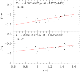
Figure 1: Transformation relations in the $V$ and $I$ band-passes between the instrumental and the standard photometric systems using a set of standard stars in the field of NGC 6229 kindly provided by Peter Stetson.

We constructed two reference images, one in the $V$ filter and another in $I$. For each of these reference images, 5 calibrated images were stacked with total exposure times of 1800 and 370 seconds in the $V$ and $I$ filters, respectively, and with PSF FWHMs of $\sim$5.2 and $\sim$4.0 pix, respectively. In each reference image, we measured the fluxes (referred to as reference fluxes) and positions of all PSF-like objects (stars) by extracting a spatially variable (with a third-degree polynomial) empirical PSF from the image and fitting this PSF to each detected object. The detected stars in each image in the time-series were matched with those detected in the corresponding reference image, and a linear transformation was derived which was used to register each image with the reference image.

Table 2: Time-series $V$ and $I$ photometry for all the confirmed variables in our field of view. Filter and epoch of mid-exposure are listed in columns 2 and 3, respectively. The standard $M_{\mbox{\scriptsize std}}$ and instrumental $m_{\mbox{\scriptsize ins}}$ magnitudes are listed in columns 4 and 5, respectively, corresponding to the variable star in column 1. The uncertainty on $m_{\mbox{\scriptsize ins}}$ is listed in column 6, which also corresponds to the uncertainty on $M_{\mbox{\scriptsize std}}$. For completeness, we also list the quantities $f_{\mbox{\scriptsize ref}}$, $f_{\mbox{\scriptsize diff}}$ and $p$ from Equation 1 in columns 7, 9 and 11, along with the uncertainties $\sigma_{\mbox{\scriptsize ref}}$ and $\sigma_{\mbox{\scriptsize diff}}$ in columns 8 and 10. This is an extract from the full table, which is available with the electronic version of the article (see Supporting Information).

Variable	Filter	HJD	$M_{\mbox{\scriptsize std}}$	$m_{\mbox{\scriptsize ins}}$	$\sigma_{m}$	$f_{\mbox{\scriptsize ref}}$	$\sigma_{\mbox{\scriptsize ref}}$	$f_{\mbox{\scriptsize diff}}$	$\sigma_{\mbox{\scriptsize diff}}$	$p$
Star ID		(d)	(mag)	(mag)	(mag)	(ADU s-1)	(ADU s-1)	(ADU s-1)	(ADU s-1)
V1	V	2455294.32981	17.971	19.087	0.009	179.343	0.957	+26.504	0.931	0.5048
V1	V	2455294.34033	18.017	19.133	0.007	179.343	0.957	+26.841	0.923	0.6244
⋮	⋮	⋮	⋮	⋮	⋮	⋮	⋮	⋮	⋮	⋮
V1	I	2455294.31704	17.435	18.422	0.029	328.424	2.483	+44.876	4.482	0.4514
V1	I	2455294.32313	17.432	18.418	0.023	328.424	2.483	+52.696	4.111	0.5226
⋮	⋮	⋮	⋮	⋮	⋮	⋮	⋮	⋮	⋮	⋮
V2	V	2455294.32981	18.140	19.251	0.011	194.212	0.956	+2.550	0.944	0.5048
V2	V	2455294.34033	18.147	19.259	0.009	194.212	0.956	+2.271	0.942	0.6244
⋮	⋮	⋮	⋮	⋮	⋮	⋮	⋮	⋮	⋮	⋮
V2	I	2455294.31704	17.530	18.514	0.032	336.249	3.188	+25.571	4.560	0.4514
V2	I	2455294.32313	17.552	18.536	0.026	336.249	3.188	+25.545	4.237	0.5226
⋮	⋮	⋮	⋮	⋮	⋮	⋮	⋮	⋮	⋮	⋮

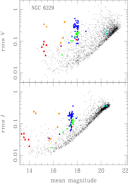
Figure 2: The rms magnitude deviations as a function of the mean magnitudes $V$ and $I$. Blue and green circles are used for RRab and RRc stars respectively. Other symbols are: red circle, V36 reclassified as RRc in this paper; orange circles, CWA, CWB or CW?; red triangles, SR; turquoise triangles, variable blue stragglers; red crosses, previously suspected variables not confirmed in this paper.

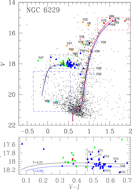
Figure 3: The top panel shows the colour-magnitude diagram of NGC 6229. Symbols and colours are as in Fig. 2. All variables labelled with numbers larger than 48 are new variables announced in the present work. See the text for a discussion on individual stars. The three dashed boxes are regions where individual star light curves were explored for variability. The isochrones are from the Victoria-Regina stellar models (VandenBerg et al. 2014) for an age of 12 Gyr and [Fe/H]=$-1.42$ (red) and $-1.31$ (blue) respectively. The bottom panel is a blow-up of the HB region, where triangles represent stars with amplitude modulations and the two vertical black lines are two empirical loci of the border between RRab and RRc distributions seen in NGC 5024 (solid) and NGC 4590 (dashed) after considering the corresponding reddenings (see the discussion in $\S$ 5). Two ZAHB models calculated from the Victoria-Regina stellar models for [Fe/H]=$-1.42$, [$\alpha$/Fe]=+0.4 and two values of helium content $Y$ 0.25 and 0.27 are included (see the discussion in $\S$ 5).

For each filter, a sequence of difference images was created by subtracting the relevant reference image, convolved with an appropriate spatially variable kernel, from each registered image. The spatially variable convolution kernel for each registered image was determined using bilinear interpolation of a set of kernels that were derived for a uniform 6$\times$6 grid of subregions across the image.

The differential fluxes for each star detected in the reference image were measured on each difference image. Light curves for each star were constructed by calculating the total flux $f_{\mbox{\scriptsize tot}}(t)$ in ADU/s at each epoch $t$ from:

$$f_{\mbox{\scriptsize tot}}(t)=f_{\mbox{\scriptsize ref}}+\frac{f_{\mbox{\scriptsize diff}}(t)}{p(t)},$$ (1)

where $f_{\mbox{\scriptsize ref}}$ is the reference flux (ADU/s), $f_{\mbox{\scriptsize diff}}(t)$ is the differential flux (ADU/s), and $p(t)$ is the photometric scale factor (the integral of the kernel solution). Conversion to instrumental magnitudes was achieved using:

$$m_{\mbox{\scriptsize ins}}(t)=25.0-2.5\log\left[f_{\mbox{\scriptsize tot}}(t)\right],$$ (2)

where $m_{\mbox{\scriptsize ins}}(t)$ is the instrumental magnitude of the star at time $t$. Uncertainties were propagated in the correct analytical fashion.

The above procedure and its caveats have been described in detail in Bramich et al. (2011), to which the interested reader is referred for further details.

2.3 Photometric Calibrations

2.3.1 Relative calibration

All photometric data suffer from systematic errors to some level that sometimes may be severe enough to be mistaken for bona fide variability in light curves. However, multiple observations of a set of objects at different epochs, such as time-series photometry, may be used to investigate, and possibly correct, these systematic errors (see for example Honeycutt 1992). This process is a relative self-calibration of the photometry, which is being performed as a standard post-processing step for large-scale surveys (e.g. Padmanabhan et al. 2008; Regnault et al. 2009).

We apply the methodology developed in Bramich & Freudling (2012) to solve for the magnitude offsets $Z_{k}$ that should be applied to each photometric measurement from the image $k$. In terms of DIA, this translates into a correction (to first order) for the systematic error introduced into the photometry from an image due to an error in the fitted value of the photometric scale factor $p$. We found that, for either filter, the magnitude offsets that we derive are of the order of $\sim 0.04$ mag with $\sim 10$% of worse cases reaching $\sim 0.2$ mag. Applying these magnitude offsets to our DIA photometry improves the light curve quality, especially for the brighter stars.

2.3.2 Absolute calibration

Standard stars in the field of NGC 6229 were not included in the online collection of Stetson (2000) at the time of preparing this paper. However, Prof. Stetson kindly provided us with a set of preliminary standard stars which we have used to transform instrumental $vi$ magnitudes into the standard VI system.

The standard minus the instrumental magnitudes show mild dependences on the colour, as can be seen in Fig.1. The transformations are of the form:

$$V_{std}=v+0.112(\pm 0.026)(v-i)-1.177(\pm 0.033),$$ (3)

$$I_{std}=i+0.066(\pm 0.018)(v-i)-1.022(\pm 0.023).$$ (4)

All of our VI photometry for the variable stars in the FoV of our collection of images of NGC 6229 is provided in Table 2. Just a small portion of this table is given in the printed version of this paper, while the full table is only available in electronic form.

Fig. 2 shows the rms magnitude deviation in our $V$ and $I$ light curves, after the application of the relative photometric calibration of Section 2.3.1, as a function of the mean magnitude.

To help us discuss the variable star search and classifications, we have built the colour-magnitude diagram (CMD) of Fig. 3 by calculating the inverse-variance weighted mean magnitudes of ∼2113 stars with $V$ and $I$ magnitudes. For better precision, the periodic variables like RRL and SX Phe are plotted using their intensity-weighted mean magnitudes $<V>$ and colours $<V>-<I>$. The use of $<V-I>$ instead does not produce a significant difference in the plotting on the CMD as they differ from $<V>-<I>$ within 0.01 mag. The regions marked on the plot, individual stars, and the HB inset will be discussed below in the corresponding sections.

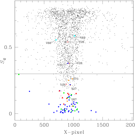
Figure 4: Minimum value of the string-length parameter $S_{Q}$ calculated for the 2113 stars with a light curve in our $V$ reference image, versus the CCD $X$-coordinate. Colours are as in Fig. 2. The horizontal line is an arbitrarily defined threshold below which most variables seem to fall. All stars below the threshold were individually explored for variability. The only true variables above the threshold are one SX Phe (V68), one unclassified variable blue straggler (V69), and one noisy RRab (V30).

2.4 Astrometry

A linear astrometric solution was derived for the $V$ filter reference image by matching 84 hand-picked stars with the UCAC4 star catalogue (Zacharias et al. 2013) using a field overlay in the image display tool GAIA (Draper 2000). We achieved a radial RMS scatter in the residuals of $\sim$0.2 arcsec. The astrometric fit was then used to calculate the J2000.0 celestial coordinates for all of the confirmed variables in our field of view (see Table 3). The coordinates correspond to the epoch of the $V$ reference image which pertains to the average heliocentric Julian day of the five images used to form the reference image, 2455665.92 d.

Table 3: General data for all of the confirmed variables in NGC 6229 in the FoV of our images. Stars V49-V73 are new discoveries in this work. Label ’Bl’ is used for Blazhko variables. The number of digits quoted for $<V>$ and $<I>$ depend on the scatter and/or amplitude modulations seen in each light curve.

Variable	Variable	$<V>$	$<I>$	$A_{V}$	$A_{I}$	$P$ (days)	$\beta$	HJDmax	$P$ (days)	RA	Dec.
Star ID	Type	(mag)	(mag)	(mag)	(mag)	this work	(d Myr-1)	(+2 450 000)	(BCV01)	(J2000.0)	(J2000.0)
V1	RRab	17.936	17.450	1.16	0.82	0.585700	+0.120	6399.3193	0.5857	16:46:56.34	+47:29:53.3
V2	RRab-Bl	18.07	17.56	1.01	0.63	0.555239	+0.044	6357.4046	0.5553	16:46:51.62	+47:31:43.5
V3	RRab	18.13	17.59	0.89	0.67	0.575259	–0.432	5753.1692	0.5752	16:46:39.38	+47:32:19.3
V4	RRab-Bl	18.09	17.53	0.86	0.58	0.566196	–0.500	5664.3882	0.5662	16:46:53.12	+47:31:24.3
V5	RRab	18.160	17.605	1.05	0.68	0.533602	–0.056	5725.3179	0.5336	16:47:00.11	+47:32:23.0
V6	RRab-Bl	18.08	17.54	0.85	0.52	0.559349	–	6462.3056	0.5593	16:47:03.03	+47:32:20.7
V7	RRab-Bl	18.02	17.55	1.15	0.77	0.506969	–	5294.3403	0.5016	16:46:54.60	+47:30:48.8
V8	CWA	15.50	14.62	0.75	0.58	14.846	–	6462.3310	14.8405	16:46:58.33	+47:30:56.9
V9	RRab-Bl	17.95	17.46	0.86	0.63	0.542841	–0.204	6357.4281	0.5428	16:46:54.85	+47:32:17.0
V10	RRab	18.101	17.533	1.00	0.65	0.554738	–0.280	6463.3279	0.5547	16:46:55.76	+47:32:51.4
V11	RRab	18.119	17.566	0.92	0.59	0.563226	–	5752.2791	0.5632	16:47:01.08	+47:31:14.1
V12	RRab-Bl	17.91	17.67	1.16	0.95	0.490812	–	6463.3125	0.4908	16:47:02.11	+47:31:15.4
V13	RRab	18.106	17.591	0.93	0.62	0.547345	+0.056	6357.3728	0.5473	16:47:12.51	+47:32:41.0
V14	RRab	17.840	17.353	1.04	0.66	0.465926	+0.096	5725.3366	0.4659	16:46:57.21	+47:30:48.1
V15	RRc	18.12	17.72	0.52	0.32	0.271379	+0.024	5722.2369	0.2714	16:47:02.07	+47:32:06.7
V16	RRc-Bl	17.98	17.61	0.49	0.30	0.322836	+0.780	6399.2877	0.3227	16:47:03.36	+47:31:15.0
V17	RRc-Bl	17.91	17.59	0.46	0.35	0.325141	–	6463.2279	0.3252	16:46:49.25	+47:30:23.4
V18	RRab	18.066	17.497	0.79	0.51	0.579039	–	5725.3594	0.5791	16:46:55.13	+47:32:11.0
V19	RRab	18.130	17.631	1.29	0.87	0.475960	–0.024	6462.3457	0.4759	16:47:03.99	+47:30:54.9
V20	RRab-Bl	18.17	17.68	1.30	0.88	0.465952	–0.232	6046.3548	0.4660	16:46:56.03	+47:31:02.8
V21	RRab	18.063	17.546	0.98	0.66	0.564426	–	6462.3941	0.5644	16:47:10.32	+47:30:38.0
V22	CWA	15.28	14.43	0.88	0.72	15.846	–	6047.4139	15.8373	16:46:58.95	+47:31:28.1
V23	RRc	17.868	17.433	0.38	0.22	0.397688	–	5722.2369	0.3977	16:46:56.72	+47:32:36.0
V24	RRc	18.016	17.668	0.44	0.30	0.303441	–	5752.2182	0.3034	16:46:57.45	+47:30:40.5
V27	CW?	16.83	16.35	0.49	0.31	–	–	6358.3593	1.13827	16:46:59.85	+47:31:46.1
V29	RRab-Bl	18.30	17.44	1.50	0.74	0.629509	–	6357.4207	–	16:47:00.39	+47:31:41.5
V30	RRab	18.7	17.9	0.70	0.35	0.498700	–	6356.3490	–	16:46:58.63	+47:31:23.3
V31	RRab	17.77	17.24	0.88	0.61	0.537851	–	6462.3941	0.6989	16:46:59.30	+47:31:18.9
V32	RRab-Bl	18.17	17.63	0.61	0.49	0.603805	–	5752.2266	0.3765	16:46:58.34	+47:31:17.7
V33	RRab	18.26	17.60	1.24	0.78	0.517500	–	6356.3640	0.5176	16:46:58.24	+47:32:01.1
V34	RRab	18.14	17.58	0.99	0.61	0.555409	–	6356.3936	0.5554	16:47:01.43	+47:31:44.7
V35	RRab	18.062	17.501	0.31	0.23	0.634460	–	5665.3884	0.6345	16:47:01.53	+47:31:57.2
V36	RRc	17.942	17.569	0.32	0.22	0.264133	–	6399.2877	0.2641	16:46:56.51	+47:32:02.9
V37	RRab	17.947	17.482	0.83	0.63	0.519174	–	6399.4511	0.5192	16:46:58.87	+47:32:11.9
V38	RRab-Bl	18.06	17.68	1.06	0.78	0.522159	–	5665.3610	0.5222	16:46:57.09	+47:31:11.4
V39	RRc	18.113	17.678	0.42	0.31	0.332997	–	5725.3982	0.4993	16:47:03.05	+47:31:08.1
V40	RRab-Bl	17.58	17.51	0.51	0.50	0.591408	–	6399.2877	0.5914	16:47:02.37	+47:31:58.8
V41	RRab-Bl?	18.12	17.51	0.42	0.31	0.634608	–	5725.1939	0.6347	16:47:02.78	+47:31:30.4
V42	RRab	18.07	17.54	0.50	0.37	0.621730	–	5664.4199	0.6218	16:47:01.30	+47:32:00.9
V43	RRab-Bl	17.94	17.41	1.14	0.73	0.567649	–	5725.1641	0.5677	16:46:56.99	+47:32:01.8
V44	RRc	17.988	17.598	0.45	0.33	0.357365	–	6356.4737	0.3573	16:47:00.57	+47:30:51.6
V45	RRab	18.027	17.486	0.48	0.33	0.640061	–	6356.3490	0.6401	16:46:59.18	+47:30:22.2
V46	RRab	17.965	17.433	0.28	0.22	0.638741	–	6400.3493	0.6388	16:46:53.97	+47:31:24.8
V47	RRc-Bl	17.80	18.03	0.36	0.40	0.333948	–	5724.3047	0.3339	16:47:03.40	+47:31:26.5
V48	RRc	17.85	17.47	0.38	0.26	0.340270	–	5753.1385	0.5164	16:47:01.46	+47:31:20.0
V49	RRab	18.08	17.51	0.35	0.24	0.637320	–	5666.3954	–	16:46:54.75	+47:32:36.5
V50	RRab-Bl	18.11	17.80	1.25	0.96	0.492440	–	5752.3148	–	16:46:56.78	+47:31:43.9
V51	RRab	16.66	15.65	0.26	0.11	0.548110	–	5725.4078	–	16:46:57.21	+47:31:27.4
V52	RRab	18.13	17.53	1.05	0.57	0.491680	–	6356.3733	–	16:46:57.98	+47:32:02.3
V53	RRab-Bl?	18.12	17.53	0.36	0.25	0.625180	–	5753.2588	–	16:46:58.62	+47:33:41.4
V54	RRab	17.90	17.34	0.73	0.47	0.570370	–	6399.2877	–	16:46:59.20	+47:31:50.2
V55	RRab	18.00	17.37	1.19	0.64	0.525180	–	6462.3893	–	16:46:59.48	+47:31:18.1
V56	RRab	18.04	17.34	0.41	0.28	0.638310	–	6356.3490	–	16:46:59.70	+47:31:52.6
V57	RRab	18.22	17.66	0.99	0.70	0.561640	–	5753.1692	–	16:47:00.25	+47:31:31.2
V58	RRab	17.319	16.527	0.30	0.16	0.639500	–	5725.3496	–	16:47:00.34	+47:32:14.6
V59	RRc	18.0	17.7	0.55	0.21	0.335780	–	5663.4655	–	16:46:34.04	+47:32:26.0
V60	RRc	18.016	17.684	0.38	0.25	0.260380	–	6358.4103	–	16:46:55.27	+47:31:31.0
V61	RRc-Bl	17.67	17.16	0.31	0.20	0.343050	–	5753.2932	–	16:46:56.59	+47:31:41.6
V62	RRc-Bl	17.48	16.81	0.27	0.16	0.299040	–	6357.4281	–	16:46:59.52	+47:32:02.0
V63	RRc	16.750	15.893	0.12	0.05	0.341660	–	5752.2898	–	16:47:00.41	+47:31:27.6

Table 3: Continued

Variable	Variable	$<V>$	$<I>$	$A_{V}$	$A_{I}$	$P$ (days)	$\beta$	HJDmax	$P$ (days)	RA	Dec.
Star ID	Type	(mag)	(mag)	(mag)	(mag)	this work	(d Myr-1)	(+2 450 000)	(BCV01)	(J2000.0)	(J2000.0)
V64	SR	15.42	13.94	0.29	0.13	–	–	–	–	16:46:55.87	+47:31:59.9
V65	SR	15.22	13.65	0.17	0.12	–	–	–	–	16:46:58.11	+47:31:20.5
V66	SR	15.04	13.54	0.33	0.16	–	–	–	–	16:46:59.01	+47:31:58:0
V67	CWB	17.12	16.53	1.35	0.84	1.51547	–	5724.1700	–	16:47:00.83	+47:31:41.3
V68	SX Phe	20.49	20.48	0.4	–	0.0384563	–	5663.3201	–	16:46:52.57	+47:33:23.1
V69	?	20.46	20.24	0.22	–	0.271264	–	6356.3416	–	16:47:01.85	+47:32:13.3
V70	SR	15.18	13.55	0.36	0.21	–	–	–	–	16:46:54.22	+47:33:37.2
V71	SR	15.22	13.35	0.39	0.20	–	–	–	–	16:46:58.58	+47:31:36.9
V72	SR	15.35	13.99	0.12	0.10	–	–	–	–	16:47:02.81	+47:30:21.2
V73	CW?	16.62	15.78	–	–	–	–	–	–	16:47:00.85	+47:31:43.4

3 Variable stars in NGC 6229

3.1 Search for new variable stars

All previously known 48 variables were identified by their equatorial coordinates listed in the CVSGC. The main approach to identify new variables was the string-length method (Burke, Rolland & Boy 1970; Dworetsky 1983), in which each light curve is phased with periods between 0.02 and 1.7 day and a normalised string-length statistic $S_{Q}$ is calculated for each trial period. Extending the period base to values $~{}\sim 2.5$d does not produce a significantly different diagram. On the other hand if the period range is stretched to much longer periods, i.e. $>10$d, the routine tends to find multiples of the true periods for some RR Lyrae. The long period variables are to be spotted by the other methods described below. In Fig. 4 we plot the minimum $S_{Q}$ value for each light curve as a function of their corresponding CCD $X$-coordinate. The known variables are plotted with the coloured symbols described in the caption. The horizontal line is a threshold set by eye at $S_{Q}=0.30$, below which most variables seem to fall and then it is below this line where we might expect to find previously undetected variables. Then we carefully inspected for variability the light curve of each star with $S_{Q}$ below 0.30. This approach allowed us to detect the new variables now labelled V49-V67 and to confirm the non-variability of stars V26 and V28. Despite falling below the threshold, V25 does not show convincing signs of variability. We also note that this method did not work for the SX Phe star, a fact already pointed out before by Arellano Ferro et al. (2010) in the study of NGC 5024.

A second approach towards searching for variable stars was to separate the light curves of stars in a given region of the CMD where variables are expected, e.g. HB, blue stragglers region, upper instability strip and the RGB. A further more detailed inspection of stars in these regions revealed two new variables in the blue stragglers region, V68 and V69. At least star V68 can be classified as SX Phe. Also the SR variables labelled V70-V72 and a possible CW star V73, which we had missed from the string-length method, were found in this way.

Finally, we used a third approach that consisted in detecting PSF-like peaks in a stacked image built from the sum of the absolute valued difference images normalised by the standard deviation in each pixel as described by Bramich et al. (2011). This method allowed us to confirm the variability of all of the new variables discovered by the previous methods but no new variables emerged.

The confirmed variables, their mean magnitudes, amplitudes, periods, times of maximum light and equatorial coordinates are listed in Table 3. Detailed finding charts of all variables are given in Figs. 5 and 6. The light curves of RRL stars, phased with the ephemerides given in Table 3 are displayed in Figs.7 and 8. Comments on individual stars are made in Appendix A.

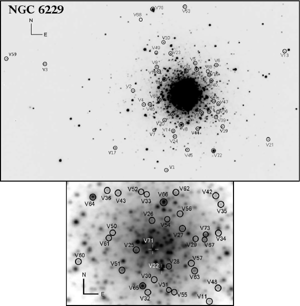
Figure 5: Finding charts constructed from our $V$ reference image; north is up and east is to the right. The cluster images are 7.3$\times$4.4 and 1.25$\times$0.90 arcmin².

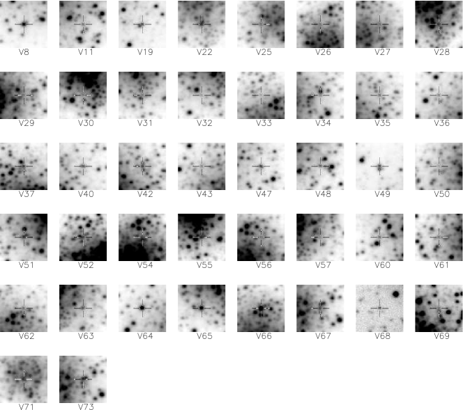
Figure 6: Finding chart of selected individual stars. Each stamp is 23.7$\times$23.7 arcsec².

From the above methods of variable star finding we estimate that our search is complete down to about $V\sim 18.5$ for amplitudes larger than 0.03 mag and periods between 0.2 d and a few tens of days in the outer regions of the cluster. However, we note that the core is very concentrated and our subtractions there are noisy. Therefore, our variable search in the core is not complete. In two recent papers Skottfelt et al. (2013; 2015) have shown the benefits of using electron multiplying CCD (EMCCD) photometry and DIA to extract faint variables in the dense central regions of globular clusters. This is achieved from a high frame-rate time-series and by shifting and adding frames to counteract the blurring atmospheric effects which contributes towards a high spatial resolution. Thus we believe the core of NGC 6229 would be an excellent target for EMCCD photometry.

Figure 7: Light curves of the RRab stars in NGC 6229. They are phased with the ephemerides listed in Table 3, the periods in days are given next to the identification. To preserve the vertical scale and limits the vertical axes display $V-<V>$ and $I-<I>$; the individual mean values are also listed in the table. Orange circles represent the data from Baade (1945) and green circles are data from Mannino (1960), whenever available. Phase differences between the archival data and our data suggest secular period variations that are calculated in $\S$ 3.2. Variables with names V49 and onwards are new discoveries in this paper.

Figure 7: Continued

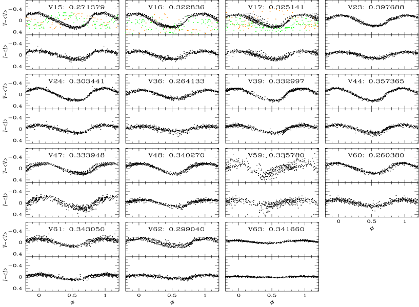
Figure 8: Light curves of the RRc stars in NGC 6229 phased with the periods listed in Table 3.

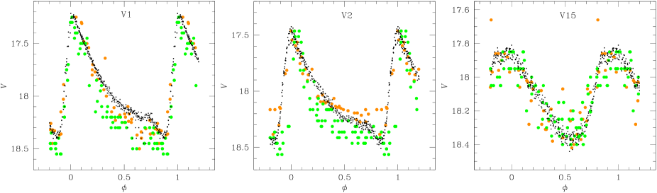
Figure 9: Examples of light curves phased with the ephemerides including the period change rate $\beta$ which are listed in Table 3. Colour symbols are as in Fig. 7.

3.2 RR Lyrae stars with a secular period variation

The combination of our data with those from Baade (1945) and Mannino (1960), available for variables V1-V21, give a time-base of about 81 years. For the benefit of future work on these variables we have uploaded these archival data into the Strasbourg astronomical Data Center (CDS). For these stars the light curves of the archival data phased with the ephemerides in Table 3 are also shown in Figs. 7 and 8. Prominent phase shifts are visible for the different data sets in several variables, suggesting secular period variations. Despite the large time-base, the number of times of maximum that can accurately be determined for each variable is limited, preventing us from calculating the secular period change with the classical O-C residuals analysis. Alternatively, we used the approach introduced by Kains et al. (2015) for the case of NGC 4590, which for completeness is described below. The period change can be represented as

$$P(t)=P_{0}+\beta(t-E),$$ (5)

where $\beta$ is the period change rate expressed in units of d d^-1, and $P_{0}$ is the period at the epoch $E$. The number of cycles at time $t$ elapsed since the epoch $E$ is:

$$N_{E}=\int_{E}^{t}\frac{dx}{P(x)}=\frac{1}{\beta}{\rm ln}[1+\frac{\beta}{P_{0}}(t-E)],$$ (6)

hence the phase at time $t$ can be calculated as

$$\phi(t)=N_{E}-{\left\lfloor N_{E}\right\rfloor}.$$ (7)

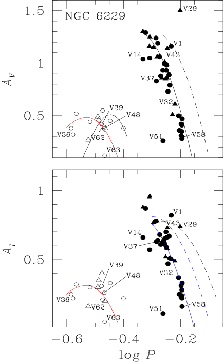
Figure 10: The log P vs. amplitude plane for the $V$ and $I$ amplitudes of the RRL in NGC 6229. Filled and open symbols represent RRab and RRc stars respectively. Triangles are used for stars with Blazhko modulations. In the top panel the continuous and segmented lines are the loci found by Cacciari et al. (2005) for unevolved and evolved RRab stars, respectively, in the OoI cluster M3. The black parabola was found by Kunder et al. (2013b) from 14 Oo II clusters. We calculated the red parabola from a sample of RRc stars in five Oo I clusters and avoiding Blazhko variables. In the bottom panel the black segmented locus was found by Arellano Ferro et al. (2011, 2013) for the OoII clusters NGC 5024 and NGC 6333. The blue loci are from Kunder et al. (2013a) for the OoI cluster NGC 2808. The red parabola was calculated from RRc stars in three Oo I clusters with $I$ amplitudes.

Then we construct a grid ($P$,$\beta$) with values in steps of $10^{-6}d$ and 0.004 d Myr^-1 in $P$ and $\beta$ respectively, around a given starting period $P_{0}$, and examine the light curve dispersions for each pair. We choose as a solution the one that produces the minimum dispersion of our data combined with those of Baade (1945) and Mannino (1960). In Fig. 9 we show three examples of the light curves phased with eq. 7, those of the RRab stars V1 and V2 and the RRc V15. The resulting $P$ and $\beta$ for those stars with an evident period change are listed in Table 3. In a few cases where the archival data are very scattered, we have not been able to find a reliable solution (e.g. for stars V17 and V18); however, their secular variation is clear and the proper calculation will have to wait until sufficient data become available.

The period change rates that we found are very scattered; they average $-0.116\pm 0.201$ d Myr^-1. While this number is consistent with zero, the scatter is very large. Taking the sign of the period change rate as an indication of the direction in which the star is evolving, we could not discern for NGC 6229 a systematic direction towards which stars are evolving. A summary of the observed period changes in RR Lyrae stars in globular clusters is offered by Catelan (2009), in particular his Fig. 15, according to which the period change rate $\beta$ is related to the ${\cal L}={\rm(B-R)/(B+V+R)}$ Lee-Zinn parameter, defined to describe the stellar distribution on the HB (Zinn 1986; Lee 1990), where B, V, R refer to the number of stars to the blue, inside and to the red of the RR Lyrae instability strip. Catelan’s diagram shows that, for clusters with ${\cal L}<0.5$ the value of $\beta$ is negligible, and it increases exponentially for larger ${\cal L}$, i.e. for clusters with blue HB’s. From star counts in our CMD we estimate for NGC 6229 ${\cal L}=0.18$, which can be compared with the value 0.24 reported by Mackey & van den Bergh (2005), and that would imply $\beta\sim 0.$ Despite this the average $\beta$ found in this paper is very negative but with a large scatter. This may imply that rather erratic period changes dominate the period changes produced otherwise by stellar evolution across the instability strip in NGC 6229.

3.3 Bailey diagram and Oosterhoff type

The periods of the 42 RRab and 15 RRc stars listed in Table 3 average 0.561d and 0.322d, respectively. These values clearly indicate that NGC 6229 is an Oosterhoff type I cluster.

The Bailey diagram for the $V$ and $I$ filters is shown in Fig. 10. The distribution of the RRab stars in each plane is in close agreement with the loci identified for Oo I clusters by Cacciari et al. (2005) (M3), Kunder et al. (2013a) (NGC 2808) and Arellano Ferro et al. (2014) (NGC 3201). A number of outliers are noted: the case of V51 can be understood since its amplitude is uncertain due to its Blazhko nature. For V14 and V37, with clean non-modulated light curves, we do not have an explanation. In the upper end we note V1 is the only non-modulated star sitting near the locus for evolved stars, however its position on the HB (see the bottom panel of Fig. 3) does not add to that interpretation. The Bailey diagram further confirms NGC 6229 as an Oo I type cluster.

The distribution of RRc stars is expected to have a parabolic form (Bono et al. 1997) as in fact it has been found in some Oo II clusters e.g. NGC 2419 (Di Criscienzo et al. 2011), M9 (Arellano Ferro et al. 2013), M55 (Olech et al. 1999), M30 (Kains et al. 2013) and Kunder et al. (2013b) for a group of 14 Oo II clusters. We have assembled a sample RRc stars in Oo I clusters (M3, M5, M79, NGC 6229 and NGC 6934) with determined amplitudes in $V$ and/or $I$ and without obvious amplitude modulatios. From their distribution (not shown here) we calculated the red parabolas shown in Fig. 10. The scatter about these parabolas is sometimes considerable, like in the case of Oo II clusters of Kunder et al. (2013a). The mathematical expresions for these parabolas are:

$$A_{V}=-3.95+30.17P-51.35P^{2},$$ (8)

$$A_{I}=-2.72+20.78P-35.51P^{2}.$$ (9)

4 RR Lyrae stars: [Fe/H] and M_V from light curve Fourier decomposition

Stellar physical parameters, such as [Fe/H], M_V, $T_{\rm eff}$, mass and radius for RR Lyrae stars can be calculated via the Fourier decomposition of their $V$ light curves into its harmonics as:

$$m(t)=A_{0}~{}+~{}\sum_{k=1}^{N}{A_{k}~{}\cos~{}({2\pi\over P}~{}k~{}(t-E)~{}+~{}\phi_{k})},$$ (10)

where $m(t)$ are magnitudes at time $t$, $P$ is the period and $E$ the epoch. A linear minimization routine is used to derive the amplitudes $A_{k}$ and phases $\phi_{k}$ of each harmonic, from which the Fourier parameters $\phi_{ij}=j\phi_{i}-i\phi_{j}$ and $R_{ij}=A_{i}/A_{j}$ are calculated. The mean magnitudes $A_{0}$, and the Fourier light curve fitting parameters of individual RRab and RRc stars are listed in Table  4. In this table we have excluded stars with evident amplitude modulations or excessive noise.

Table 4: Fourier coefficients $A_{k}$ for $k=0,1,2,3,4$, and phases $\phi_{21}$, $\phi_{31}$ and $\phi_{41}$, for RRab and RRc stars. The numbers in parentheses indicate the uncertainty on the last decimal place. Also listed is the deviation parameter $D_{\mbox{\scriptsize m}}$ (see Section 4).

Variable ID	$A_{0}$	$A_{1}$	$A_{2}$	$A_{3}$	$A_{4}$	$\phi_{21}$	$\phi_{31}$	$\phi_{41}$	$D_{\mbox{\scriptsize m}}$
	($V$ mag)	($V$ mag)	($V$ mag)	($V$ mag)	($V$ mag)
					RRab stars
V1	17.936(1)	0.383(2)	0.206(2)	0.132(2)	0.088(2)	3.988(12)	8.316(18)	6.422(26)	0.9
V5	18.160(2)	0.359(2)	0.174(2)	0.128(2)	0.081(2)	3.876(18)	8.099(27)	6.153(37)	2.0
V10	18.101(2)	0.332(2)	0.158(2)	0.120(2)	0.075(2)	3.894(18)	8.198(25)	6.232(38)	1.0
V11	18.119(3)	0.302(3)	0.151(3)	0.102(2)	0.065(3)	4.043(29)	8.386(43)	6.526(63)	0.4
V13	18.106(2)	0.308(3)	0.159(3)	0.112(2)	0.069(2)	3.886(25)	8.238(36)	6.235(53)	1.4
V14	17.840(2)	0.366(3)	0.182(3)	0.125(3)	0.078(3)	3.737(22)	7.790(32)	5.681(48)	1.9
V18	18.066(2)	0.273(2)	0.128(2)	0.091(2)	0.052(2)	4.124(24)	8.420(36)	6.823(56)	3.7
V19	18.130(2)	0.432(3)	0.209(3)	0.153(3)	0.101(3)	3.811(20)	7.957(29)	5.906(42)	1.5
V21	18.063(2)	0.304(3)	0.152(3)	0.105(3)	0.070(3)	4.011(32)	8.293(47)	6.308(95)	1.5
V35	18.062(1)	0.115(2)	0.039(2)	0.020(2)	0.002(2)	4.259(64)	8.924(111)	7.049(84)	6.0
V37	17.947(2)	0.282(3)	0.138(3)	0.095(3)	0.057(3)	3.959(29)	8.171(43)	6.237(63)	1.1
V45	18.027(1)	0.174(2)	0.073(2)	0.037(2)	0.014(2)	4.190(31)	8.794(55)	7.540(13)	26.9
V46	17.965(1)	0.115(2)	0.039(2)	0.018(2)	0.009(2)	4.280(31)	9.042(55)	7.899(13)	32.5
V51	16.658(1)	0.068(2)	0.040(2)	0.031(2)	0.022(2)	4.050(71)	8.312(101)	6.436(183)	4.1
V58	17.319(1)	0.102(1)	0.046(1)	0.023(1)	0.007(1)	4.046(14)	8.664(14)	7.056(13)	4.1
					RRc stars
V15	18.118(2)	0.252(2)	0.056(2)	0.015(2)	0.014(2)	4.635(43)	2.716(158)	1.449(167)	–
V23	17.868(1)	0.185(2)	0.009(2)	0.011(2)	0.007(2)	5.742(211)	4.718(183)	3.143(270)	–
V24	18.016(1)	0.217(2)	0.030(2)	0.015(2)	0.014(2)	4.522(64)	3.262(124)	2.189(134)	–
V36	17.942(2)	0.149(2)	0.005(2)	0.002(2)	0.003(2)	4.609(464)	4.956(1296)	3.515(755)	–
V39	18.113(2)	0.210(2)	0.032(2)	0.018(2)	0.011(2)	4.695(71)	3.834(127)	2.525(209)	–
V44	17.988(1)	0.216(2)	0.027(2)	0.008(2)	0.010(2)	4.883(73)	4.051(246)	2.750(185)	–
V48	17.849(2)	0.182(3)	0.019(2)	0.009(2)	0.006(2)	5.726(130)	4.425(269)	1.978(420)	–
V60	18.016(2)	0.176(2)	0.027(3)	0.005(2)	0.003(3)	4.402(95)	2.649(481)	0.893(751)	–
V63	16.750(1)	0.046(1)	0.002(1)	0.004(1)	0.004(1)	4.550(89)	4.105(328)	2.100(362)	–

These Fourier parameters and the semi-empirical calibrations of Jurcsik & Kovács (1996), for RRab stars, and Morgan et al. (2007), for RRc stars, are used to obtain [Fe/H]_ZW on the Zinn & West (1984) metallicity scale which have been transformed to the UVES scale using the equation [Fe/H]_UVES= $-0.413$ +0.130[Fe/H]${}_{\rm ZW}-0.356$[Fe/H]${}_{\rm ZW}^{2}$ (Carretta et al. 2009). The absolute magnitude $M_{V}$ can be derived from the calibrations of Kovács & Walker (2001) for RRab stars and of Kovács (1998) for the RRc stars; these two calibrations are naturally based on different sets of calibrators in assorted Galactic and LMC globular clusters and are therefore independent. However, their zero points have been tied to the LMC distance modulus of 18.5$\pm$0.1 mag (e.g. Clementini et al. 2003) as discussed in detail by Arellano Ferro et al. (2010). The effective temperature $T_{\rm eff}$ was estimated using the calibration of Jurcsik (1998). For brevity we do not explicitly present here the above mentioned calibrations; however, the corresponding equations, and most importantly their zero points, have been discussed in detail in previous papers (e.g. Arellano Ferro et al. 2011; 2013) and the interested reader is referred to them.

It is pertinent to recall that the calibration for [Fe/H] for RRab stars of Jurcsik & Kovács (1996) is applicable to RRab stars with a deviation parameter $D_{m}$, defined by Jurcsik & Kovács (1996) and Kovács & Kanbur (1998), not exceeding an upper limit. These authors suggest $D_{m}\leq 3.0$. The $D_{m}$ is listed in column 10 of Table 4. However we have relaxed the criterion to include three stars with 3.7 $\leq D_{m}\leq$ 4.1. Those RR Lyrae that fall off the HB, discussed in $\S$ A, are not included for the luminosity calculation as indicated in the footnote of Table 5.

It is noteworthy at this stage that there is a new calibration of [Fe/H]_UVES for RRc stars, calculated for an extended number of stars and clusters by Morgan (2013). As described in her paper the results of the new calibration are in general consistent with the old calibration from Morgan et al. (2007), and that the average differences are 0.02 dex. We have also carried out the calculation using the new calibration and found [Fe/H]${}_{\rm UVES}=-1.37$, i.e. 0.08 dex more deficient than the value from the calibration of Morgan et al. (2007), which is in better agreement with the result from the RRab calibration.

Table 5: Physical parameters for the RRab and RRc stars. The numbers in parentheses indicate the uncertainty on the last decimal place.

Star	[Fe/H]UVES	$M_{V}$	log $T_{\rm eff}$	log$(L/{\rm L_{\odot}})$	$M/{\rm M_{\odot}}$	$R/{\rm R_{\odot}}$
			RRab stars
V1	$-1.385(18)$	0.511(3)	3.809(7)	1.696(1)	0.70(6)	5.69(1)
V5	$-1.394(27)$	0.611(3)	3.812(8)	1.656(1)	0.70(7)	5.36(1)
V10	$-1.378(25)$	0.604(3)	3.810(8)	1.658(1)	0.68(7)	5.42(1)
V11	$-1.215(39)$	0.612(4)	3.811(10)	1.655(2)	0.66(8)	5.40(2)
V13	$-1.302(34)$	0.636(4)	3.811(9)	1.645(2)	0.66(7)	5.32(1)
V14	$-1.437(32)$	0.711(4)	3.817(9)	1.616(2)	0.71(7)	5.00(1)
V18	$-1.245(33)$	0.614(3)	3.806(9)	1.655(1)	0.66(7)	5.50(1)
V19	$-1.297(27)$	0.640(4)	3.820(8)	1.644(2)	0.73(7)	5.10(1)
V21	$-1.317(45)$	0.610(4)	3.810(13)	1.656(2)	0.66(10)	5.42(2)
V35a	–	0.664(3)	3.804(12)	1.634(1)	0.56(8)	5.43(1)
V37	$-1.254(40)$	0.696(4)	3.813(10)	1.622(2)	0.65(8)	5.15(2)
V45a	–	0.602(3)	3.799(7)	1.659(1)	0.63(5)	5.72(1)
V46a	–	0.657(3)	3.800(21)	1.637(1)	0.58(15)	5.55(1)
V51b	$-1.229(92)$	–	3.804(21)	–	–	–
V58b	$-1.243(13)$	–	3.797(7 )	–	–	–
Weighted
Mean	$-$1.31(1)	0.621(1)	3.810(2)	1.652(1)	0.66(2)	5.43(1)
			RRc stars
V15	$-1.22(25)$	0.603(2)	3.872(1)	1.659(1)	0.61(1)	4.09(1)
V23	$-1.49(47)$	0.464(9)	3.859(1)	1.714(4)	0.47(1)	4.62(2)
V24	$-1.33(23)$	0.577(3)	3.868(1)	1.669(1)	0.56(1)	4.21(1)
V36a	–	0.660(21)	3.887(8)	1.636(8)	0.50(5)	3.72(4)
V39	$-1.34(26)$	0.555(3)	3.865(1)	1.678(1)	0.52(1)	4.31(1)
V44	$-1.50(58)$	0.527(3)	3.862(1)	1.689(1)	0.50(1)	4.43(1)
V48	$-1.03(46)$	0.524(6)	3.867(2)	1.690(2)	0.51(1)	4.33(1)
V60	$-1.11(69)$	0.673(4)	3.874(3)	1.631(2)	0.58(2)	3.92(1)
V63b	$-1.27(66)$	–	3.865(2)	–	–	–
Weighted
Mean	$-$1.29(12)	0.581(1)	3.867(1)	1.668(1)	0.54(1)	4.18(1)

^a: No [Fe/H] estimate since $D_{m}>4.1$. V36 has a very peculiar value of $\phi_{31}$; ^b: No $M_{V}$ estimate since star falls off the HB.

The physical parameters for the RR Lyrae stars and the inverse-variance weighted means are reported in Table 5. Two independent estimations of [Fe/H]_UVES have been found from 12 RRab and 8 RRc stars in NGC 6229: $-1.31\pm 0.01$ and $-1.29\pm 0.12$ respectively.

The weighted mean $M_{V}$ values for the RRab and RRc stars are 0.621$\pm$0.001 mag and 0.581$\pm$0.001 mag respectively and will be used in section 6 to estimate the mean distance to the parent cluster.

5 On the structure of the Horizontal Branch

In this section we analyse the distribution of RRL stars in the HB. The expanded HB in Fig. 3 displays in detail the positions of most of the RR Lyrae stars. RRab and RRc are distinguished as well as Blazhko and stable variables. There is a neat segregation between stable RRab and RRc with a border at $(V-I)_{0}\sim 0.45$. Similarly clear segregations have been found before in NGC 5024 (Arellano Ferro et al. 2011; their Fig. 4) and NGC 4590 (Kains et al. 2015; their Fig. 11) both at $(V-I)_{0}\sim 0.45-0.46$. In the bottom panel of Fig. 3 the corresponding border lines for NGC 5024 and NGC 4590 duly reddened are indicated. It can be seen that the border line between stable RRab and RRc is the same in the three clusters. We should emphasise that the above empirical border is trespassed by a few Blazhko variables (NGC 6229) and the double mode RRL (NGC 4590). Looking for this segregation effect in clusters previously studied by our group, we checked the CMDs and noted that with very few exceptions the effect is also visible in NGC 5053 (Arellano Ferro et al. 2010; Fig. 8) (except for V10 with a poor I light curve), NGC 1904 (Kains et al. 2012) and NGC 7099 (Kains et al. 2013), despite their low number of RRL. On the other hand the RRab-RRc splitting is definitely not seen in NGC 3201 (Arellano Ferro et al. 2014).

It is illustrative to display the HB in the $T_{\rm eff}$-${\rm log}L$ plane. In order to convert the observational HB shown in Fig. 3 into the HR diagram, we have proceeded as in Arellano Ferro et al. (2010) where a polynomial for $T_{\rm eff}$-$(V-I)_{0}$ is given based on the HB models of VandenBerg et al. (2006) with the colour-$T_{\rm eff}$ relations as described by VandenBerg & Clem (2003). Fig. 11 illustrates the distribution of RRL using the same colour code as in Fig. 3. The red and blue borders of the instability strip (IS) for the fundamental mode (F) and first overtone (FO), calculated by Nemec et al. (2011) based on the Warsaw pulsation code for a mass of 0.65 $M_{\odot}$, are shown in the figure. The two vertical black lines correspond to the empirical border between RRab and RRc stars seen in NGC 5024 (solid) and NGC 4590 (dashed) which match the evident border in NGC 6229 and that, in our opinion, represent the empirical red border of the first overtone instability strip (FORE). This is some 100-200K hotter than the theoretical border found by Nemec et al. (2011). Another feature is that the fundamental red edge (FRE) in NGC 6229 extends further to the red by at least 400K.

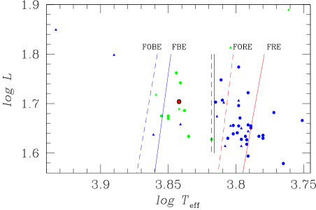
Figure 11: The HR diagram of the horizontal branch of NGC 6229. The coloured lines are the IS borders for the fundamental mode (FM) and the first overtone (FO) according to Nemec et al. (2011). The two vertical black lines correspond to the empirical border between RRab and RRc stars seen in NGC 5024 (solid) and NGC 4590 (dashed). See also Fig. 3 and the text for a discussion.

Regarding the distribution of RRc stars, they are well constrained to the first overtone instability strip. The distribution of RRL on the HB observed in NGC 6229 can be explained by the arguments of Caputo et al. (1978) which involve the occurrence of a hysteresis mechanism (van Albada & Baker 1973) for stars crossing the IS. According to this mechanism the stars in the ”either-or” region can retain the mode they were pulsating in before entering the region which depends on whether the star is coming from the blue side as a RRc or from the red side as a RRab. Furthermore, Caputo et al. (1978) suggest that the original mode in which a RRL is pulsating depends on the location of the starting point at the Zero Age Horizontal Branch (ZAHB), which in turn depends on the mass and the chemical composition of the star; they used these ideas to explain the existence of the two Oosterhoff groups. A schematic and clear explanation of this can be found in their Fig. 3. In summary there are two scenarios; 1) the ZAHB point is in the fundamental zone, leading to an assortment of RRc and RRab in the ”either-or” region and a lower value of the average period for both RRc and RRab and a lower proportion of RRc stars, hence an OoI cluster, and 2) the ZAHB point is bluer than the fundamental zone, in the ”either-or” or in the first overtone regions, then the ”either-or” region is populated exclusively by RRc stars and the RRab stars are to be found only in the fundamental region, producing larger averages of periods and a higher proportion of RRc and hence OoII type cluster.

The above scenario seems to explain well the clean segregation of RRc and RRab in OoII clusters with evolution across the IS towards the red. In agreement with this picture we can mention the analysis of Pritzl et al. (2002b). These authors have shown how in clusters with blue HBs, i.e. large values of $\cal L$, stars with masses below a critical mass on the ZAHB to the blue of the IS, evolve redwards and spend sufficient time to contribute to the population of RRL. These arguments suggest then that clusters with a blue HB morphology are OoII, with redwards evolution, which in turn favours the segregation between RRc and RRab at the IS.

We have explored the CMD of several OoII clusters published by our group over the last few years (e.g. NGC 288, NGC 1904, NGC 5024, NGC 5053, NGC 5466, NGC 6333, NGC 7099) and noted the clear segregations, with a few exceptions of indiviual stars with noisy light curves. The one exception is NGC 4590, a clear OoII with a red HB ($\cal L$=0.17) and evidences, from the secular period changes analysis of 14 RRL, that evolution does not occur in a preferential direction (Kains et al. 2015). On the other hand the OoI cluster NGC 3201 ($\cal L$=0.08) as expected, shows no signs of segregation (Arellano Ferro et al. 2014). Likewise NGC 6229 has a low $\cal L$ (0.24) and no preferential evolution direction from the scattered period change rate found in $\S$ 3.2, in spite of this the RRc and the RRab are neatly separated.

A close inspection of the distribution of clusters of all Oosterhoff types on the [Fe/H]-$\cal L$ plane from the data in Table 3 of Catelan (2009), reveals NGC 4590 as the OoII cluster with the reddest HB with ${\cal L}<0.4$ and that there are five OoI clusters (NGC 6266, NGC 6284, NGC 6402, NGC 6558 and NGC 6626) with blue HB’s (${\cal L}>0.4$). It would be of great interest to explore their RRL distributions in the IS.

One more point of interest in Fig. 11 is the distribution of Blazhko variables. We have plotted with triangles only stars that show clear Blazhko amplitude modulations while marginal cases (e.g. V50, V52, V54) are plotted as stable stars. In his paper Gillet (2013) concluded that the Blazhko effect is not a consequence of the transition between modes and that a star that penetrates the ”either or” region (RRc or RRab) becomes a Blazhko variable, as seems to be supported by the field Blazhko RRL plotted in Gillet’s Fig. 1. The later statement implies that all stars in the ”either or” region should be Blazhko variables, which is not observationally supported by the distribution of Blazhko stars in NGC 4590, NGC 5024 and NGC 6229. Some outlier Blazhko variables from the IS in NGC 6229, mostly RRab stars, are likely not the result of hysteresis in the change of mode process as once suggested by Arellano Ferro et al. (2010) but rather a consequence of multi-shock perturbation at the main pulsation instability yet to be explained by theory (e.g. Gillet 2013).

In the CMD of Fig. 3 we have overplotted two versions of the ZAHB for [Fe/H]=$-1.42$ and [$\alpha$/Fe]=+0.4; for Y=0.25 and Y=0.27, calculated from the Victoria-Regina stellar models of VandenBerg et al. (2014). The model for Y=0.25 is a reasonable lower envelope to the distribution of RRL. The difference with a non-diffusive model for [Fe/H]=$-1.31$, [$\alpha$/Fe]=+0.3 and Y=0.25 from VandenBerg et al. (2006) is negligible. Apparently the change in the primordial helium content largely compensates for the difference between diffusive and non-diffusive models (VandenBerg private communication). The only two stable RRab’s a little below this ZAHB are V33, which shows some scatter near minimum, and V55 whose flux is likely contaminated by its neighbour V31 (see the discussion in $\S$ A.0.1). If the intrinsic thickness of the stellar distribution on the HB is between 0.1-0.2 mag, e.g. the case of M3 in Fig. 1 of Cacciari et al. (2005), it is clear that a number of RRL in NGC 6229 are overluminous. A natural explanation would be evolution off the ZAHB, however we did not find evidence of stars evolved in the amplitude-period diagram of Fig. 10. Also no evidence of systematic secular period increases in this rather red-HB cluster have been found (see $\S$ 3.2). Furthermore, stars in an advanced evolution towards the AGB should be brighter and have longer periods, however we find no correlation between $<V>$ and period for the RRL in NGC 6229.

Figure 12: Period-colour diagram of stable RRL stars. Filled circles are used for RRab stars and empty circles for RRc stars. The periods of the RRc stars were fundamentalized by adding 0.127 to $\log P$. The reduced period $P^{\prime}$ is defined as $\log P^{\prime}=\log P+0.336(<V>-18.021)$. See text for further discussion.

There may be other reasons for overluminosity than evolution off the ZAHB. For example, helium abundance dispersion in HB stars could be produced if more than one generation of stars are mixed in a given GC. D’Antona & Caloi (2008) have argued that second-generation stars, formed from enriched material of first-generation progenitors, may have a spread in Y above the primordial value, and that these stars will occupy a bluer position on the HB than the first-generation ones, which sit to the red of the instability strip. It has been noted by Catelan et al. (2009) that HB stars with higher Y should also be brigther due to their stronger H-burning shells, and they have searched for such an effect in M3. By comparing with HB models with Y in the range 0.23-0.28, they concluded that no systematic overluminosity in blue HB stars is evident, and hence the Y spread in M3 should not be larger than 0.01. For NGC 6229 we have overplotted ZAHB models from VandenBerg (2014) for Y = 0.25, 0.27, and 0.285, and found no evidence of the blue HB stars being brighter than the red ones, so no spread in the value of Y is immediately obvious in this cluster either. Similar tight constraints would apply to the case of helium mixing on the RGB phase (Sweigart 1997).

Another reason may be the presence of an unseen companion. In this context it is of interest to explore the period-colour relation for stable RRL of Fig. 12. In this diagram the period ${\rm log}P^{\prime}={\rm log}P+0.336(<V>-18.021)$ where 18.021 mag is the average $<V>$ for all the stable RRL. The concept of ${\rm log}P^{\prime}$ was introduced by van Albada & Baker (1971) and it was later slightly modified by Bingham et al. (1984). It significantly reduces the scatter in the period-colour diagram and is useful for identifying stars with peculiar photometric properties such as colours too red or too blue, and luminosities too bright or too faint relative to what is expected from their periods. In Fig. 12 we note some outliers and have labelled them. V33 has been commented on above, while V36 was believed to be an RRd in the CVSGC but classified here as an RRc with a very short period among RRc stars. It is worth noting that V14, V31, V54 and V55 are also the brightest stable RRab in the HB (see the bottom panel of Fig. 3). Their position on Fig. 12 implies that they have too short a period for their colour, which implies that they have larger gravity and should be of lower luminosity. The fact that instead they are among the brightest in the HB, implies that they have an extra source of luminosity and this may be an unseen companion. It was through the same lines of argumentation that Cacciari et al. (2005) seem to have identified three RRL in M3 (V48, V58 and V146) that may have companions.

Thus it seems likely that not only evolution has contributed to the large dispersion of RRL in the HB of NGC 6229 but also a dispersion in the primordial helium abundance and in some cases the presence of unseen companions.

6 NGC 6229 distance and metallicity from its variable stars

Four independent estimates of the distance to the cluster are possible from our data; from the weighted mean $M_{V}$, calculated for the RRab and RRc from the Fourier light curve decomposition (Table 5), which can be considered as independent since they come from different empirical calibrations; from the one known SX Phe star and the P-L relation; and from the tip of the RGB bolometric magnitude calibration. Below we expand on these solutions.

Since NGC 6229 is a high Galactic latitude object and despite its large distance, the interstellar extinction and reddening are negligible, we adopted $E(B-V)$=0.01 (Harris 1996). Given the mean $M_{V}$ for RRL in Table 5 we found a true distance modulus of $17.385\pm 0.117$ mag and $17.433\pm 0.096$ mag using the RRab and RRc stars respectively, which correspond to the distances $30.0\pm 1.5$ and $30.7\pm 1.1$ kpc. The quoted uncertainties are the standard deviation of the mean. The distance to NGC 6229 listed in the catalogue of Harris (1996) (2010 edition) is 30.5 kpc in good agreement with our calculations.

A third independent estimate of the distance to the cluster is via the one SX Phe identified in this work, V68, assuming that its period 0.0384563d corresponds to the fundamental mode. We have used the P-L relation of Cohen & Sarajedini (2012);

$$M_{V}=-(1.640\pm 0.110)-(3.389\pm 0.090){\rm log}P_{f}$$ (11)

where $P_{f}$ refers to the fundamental mode given in days. The above equation implies a true distance modulus of 17.303$\pm$0.168 or a distance of $28.9\pm 2.2$ kpc. The uncertainty was calculated from calibration errors neglecting the uncertainty of the period. It is worth noting that eq. 11, when applied to a sample of $\delta$ Scuti stars in the LMC produces a distance modulus of 18.49$\pm$0.10 (Cohen & Sarajedini 2012) which is consistent with the modulus 18.5$\pm$0.1 used to set the zero points of the absolute magnitude calibrations for RRab and RRc stars (see Arellano Ferro et al. 2010 $\S$ 4.2). Thus the distances derived here for the RRL and the SX Phe are on a consistent distance scale.

Yet another approach to the cluster distance determination is by using the tip of the RGB. This method was developed for estimating distances to nearby galaxies (Lee, Freedman & Madore, 1993). Here we used the calibration of Salaris & Cassisi (1997) for the bolometric magnitude of the tip of the RGB in terms of the overall metallicity:

$$M_{bol}^{tip}=-3.949-0.178[M/{\rm H}]+0.008[M/{\rm H}]^{2}$$ (12)

where $[M/\rm H]={\rm[Fe/H]}+\rm log(0.638f+0.362)$ and log f = [$\alpha$/Fe] (Salaris et al. 1993).

We found that the method is extremely sensitive to the star selection as the tip of the RGB, hence we restricted our calculation to the five reddest stars in the red box in the CMD of Fig. 3. We have assumed [$\alpha$/Fe]=+0.4 (e.g Jimenez & Padoan 1998) and found an average distance of $34.9\pm 2.4$ kpc.

Within their own uncertainties the above distance determinations are satisfactorily in agreement. However, since the SX Phe determination is based on only one star and the tip of the RGB approach is very sensitive to the selected RGB tip stars, which in turn is scattered, we believe that the distance determination from the RRL stars is the most accurate.

The average value of [Fe/H]${}_{\rm UVES}=-1.31\pm 0.12$ found from the Fourier decomposition of the light curves of 12 RRab and 8 RRc stars in NGC 6229 compares very well with the numerous determinations in the literature. In the present edition of his catalogue of globular clusters Harris (1996) lists an average [Fe/H]${}_{\rm ZW}=-1.47$ (or [Fe/H]${}_{\rm UVES}=-1.37$) for NGC 6229. A list of individual results from an assortment of indicators can be found in Table 7 of Borissova et al. (1999); they range from $-1.26$ to $-1.44$ in the ZW scale or from $-1.14$ to $-1.34$ in the UVES scale with uncertainties running within 0.08-0.15 dex.

6.1 A brief comment on the age of NGC 6229

We have not attempted an independent estimation of the age of NGC 6229 since a thorough effort based on deep photometry has already been carried out by Borissova et al. (1999). In that paper the authors soundly argue from their differential age analysis that NGC 6229 and M5 are coeval within 1 Gyr. To the best of our knowledge no direct estimation of the absolute age of NGC 6229 has been carried out. However, the age of M5 was determined by Jimenez & Padoan (1998) via its luminosity function and they found an age of $10.6\pm 0.8$ Gyr taking into account [$\alpha$/Fe]=+0.4. Two more recent determinations of the age of M5 are by Dotter et al. (2010) using relative ages isochrone fitting and by VandenBerg et al. (2013) using an improved calibration of the ”vertical method” or the magnitude difference between the turn off point and the HB; these authors find 12.25$\pm$0.75 Gyr and 11.50$\pm$0.25 Gyr respectively. Thus, in the CMD of Fig. 3 we have overlayed the corresponding isochrones for 12.0 Gyr from the Victoria-Regina evolutionary models (VandenBerg et al. 2014) and for the metallicities [Fe/H]=$-1.42$ (red) and [Fe/H]=$-1.31$ (blue) and [$\alpha$/Fe]=+0.4, shifted for the average apparent distance modulus $\mu$=17.440 mag found from the RRab and RRc stars, and $E(V-I)=1.616~{}E(B-V)=0.016$.

The isochrones for these two metalicities are very similar except perhaps at the tip of the RGB where the richer isochrone gets less luminous. However, if a vertical shift is applied to these isochrones within the uncertainty of the distance modulus, 0.01 mag, then the two cases are indistinguishable. We can stress then that our CMD is consistent with the metallicity and distance derived in this paper and an age of 12.0$\pm$1.0 Gyr found in the above papers for the coeval cluster M5.

7 Summary of results and conclusions

We have significantly updated the census of variable stars in NGC 6229. The DIA approach to the CCD image reduction and analysis allowed us to recover all of the 48 variables previously known and to identify 25 new variables; 10 RRab, 5 RRc, 6 SR, 1 CW, 1 SX Phe and two new variables that we were unable to classify.

Numerous new Blazhko variables have been identified among both the already known and the new RRL stars, including five RRc variables (V16, V17, V47, V61 and V62) (see Table 3). Also our data do not support the Blazhko effect seen in V5, V18, V33, V34, V35, V37, V46 and V48 by BCV01 based on the $D_{m}$ parameter which is very sensitive to light curve coverage and scatter.

Thanks to the inclusion of archive data from 1932-1935 (Baade 1945) and from 1956-1958 (Mannino (1960) we have noted secular period variations in 16 RRL and have calculated the period change rate in 13 of them.

The variability of V29 and V30 is confirmed and they are classified here as RRab. On the other hand the variability of previously suspected variables V25, V26, V28 is not confirmed. The classifications of V31, V32 and V39, previously believed to be EB, RRc and RRab respectively, are now corrected as RRab, RRab and RRc.

The metallicity and distance of NGC 6229 were calculated via the light curve Fourier decomposition of RRab and RRc stars to find averages of [Fe/H]${}_{\rm UVES}=-1.31\pm 0.12$ and $d=30.3\pm 1.4$ kpc. These results agree with previous independent determinations and the observed CMD matches the above results and the isochrone of age $12.0\pm 1.0$ Gyr (Jimenez & Padoan 1998; Dotter et al. 2010; VandenBerg et al. 2013).

Regarding the RRL distribution in the HB we have stressed once more the clear splitting between stable RRc and RRab with an empirical border at about $(V-I)_{0}=0.45-0.46$ mag, clearly observed in NGC 6229 and equally clear in NGC 4590 and NGC 5024, despite being of different Oosterhoff type. This border is interpreted as the red edge of the first overtone instability strip. Blazhko variables and double mode stars do not obey that border.

Appendix A Comments on Individual Stars

In this appendix we comment on the light curves, variable types and nature of some interesting or peculiar variables in Table 3. We put some emphasis on the amplitude and phase modulations of the Blazhko type in specific stars and note that several variables catalogued as Blazhko variables by BCV01 are not confirmed by our data and that we have detected a few new ones. In their study, these authors combined older photographic data converted into $B$ magnitudes with their own $B$ DAOPHOT and ISIS photometry to evaluate the amplitude variations (see their Fig. 7 for example). Then they calculated the deviation parameter $D_{m}$, (Jurcsik & Kovács 1996; Kovács & Kanbur 1998) and for classification purposes assumed that RRab stars with $D_{m}>5$ are Blazhko variables but note however, that examples exist of Blazhko and non-Blazhko variables that do not obey such criterion as $D_{m}$ which is quite sensitive to the coverage of the light curve. In the present case, all the stars we catalogue as Blazhko variables are judged from our homogeneous data sets in the $V$ and $I$ filters, where the amplitude modulations are neatly distinguished in the light curves in Figs. 7 and 8. Hence, some inconsistencies in the identification of Blazhko variables between the two studies are expected and we make them explicit in the following paragraphs.

A.0.1 RR Lyrae stars

V2, V9, V12, V43. These stars show Blazhko modulations not identified as such by BCV01. Stars V2, and V9 also undergo secular period variations which are reported in Table 3.

V3, V59. These RRL stars display very scattered light curves despite being located in an uncrowded region. We find no evidence of either star to be blended. However, we note relatively poor image subtractions for these stars and in this area of the field, possibly due to the proximity with the image edge. These are not Blazhko modulations.

V5, V18, V33, V34, V35, V37, V46, V48. We find no evidence of amplitude modulations in these stars classified as Blazhko variables by BCV01.

V7. The star was classified as a RRab Blazhko variable by BCV01 based on its peculiar Fourier coefficients. Our data show very prominent amplitude modulations ranging about half a magnitude, but we note that RRab-like variations are preserved. Our data are insufficient to estimate the Blazhko period, but an inspection of the amplitudes and dates shows that the first amplitude decrease took place between April 11th and July 9th 2011. A new amplitude increase occurred from March 5th to June 18th, 2013, i.e. in each case the amplitude extrema were reached within 90 and 100 days.

V16, V17, V47, V61, V62. These RRc stars show evidence of amplitude and phase modulations that cannot be solved by a secular period change or explained by double mode pulsation. We consider these modulations as due to the Blazhko effect. We note that star V47 falls much to the blue from the HB. However, it is an unresolved pair (see Fig. 5) and undoubtedly its colour has been polluted by the neighbour.

V29. It was listed by Spassova & Borissova (1996) as a probable variable star and it was not included in the study of BCV01. Our data plotted in Fig. 7 clearly show a RRL type light curve with a small amplitude modulation. Thus we confirm it to be a RRab variable with the Blazhko effect. For its period (0.629509d) its amplitude in both $V$ and $I$ is peculiarly large, as seen in Fig. 10.

Figure 13: Light curves of the six new SR stars.

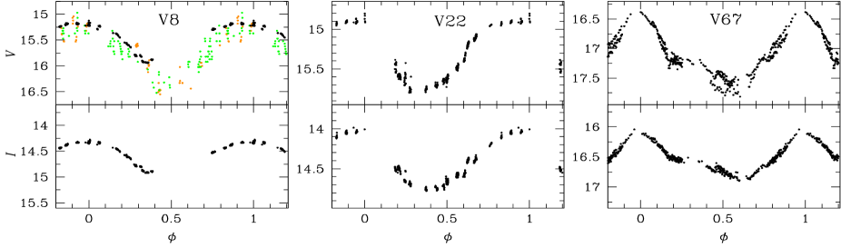
Figure 14: The three CW stars in NGC 6229 phased with their periods in Table 3. For V8 the data from Baade (1945) (orange) and Mannino (1960) (green) are included and show the stability of its period. In V67 small amplitude modulations are visible.

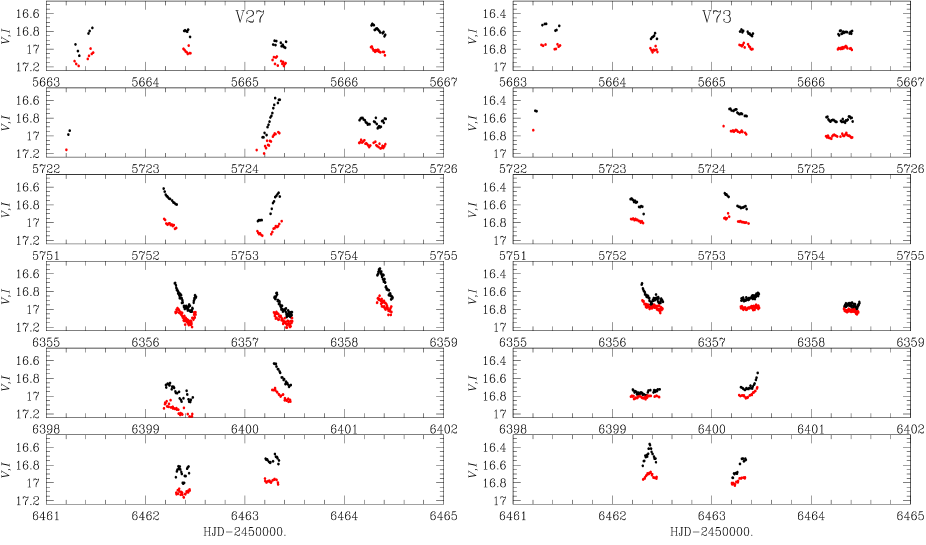
Figure 15: Light variations of the possible CW stars V27 and V73. Black and red circles are the $V$ and $I$ magnitudes respectively. The $I$ magnitudes have been arbitrarily shifted to accomodate them in the same box, so that the variations in both filters can be appreciated. Note that $V$-$I$ variations are also evident in both stars.

V30. This is a faint and blended star quite close to the cluster core displaying a very noisy light curve. Despite this, its light curve shows a RRab-like shape. The star was reported as a possible variable by Spassova & Borissova (1996) and was not included in the paper by BCV01. Hence, our light curve in Fig. 7 is the first one published for this star. We confirm the variability and suggest that the star is likely a background RRab which would be consistent with its fainter and redder position on the CMD.

V31 and V55. V31 was classified by BCV01 as an eclipsing binary with a period of 0.698893d. Our data do not phase well with that period but instead we find 0.537851d. The light curve phased with this period appears like that of a RRab star (Fig. 7). V31 is very near a new variable star identified in this work, V55, also a RRab star. The periods of these two stars are similar but not equal, since each one does not phase the light curve of the neighbouring star. Also the times of maximum do not coincide. We have confirmed that both stars are clearly variable by blinking the difference images. The amplitude modulations visible in both stars however, are most likely not authentic as the light curves of both stars may be influencing each other. Nevertheless, we do not confirm V31 as an eclipsing binary but instead we classify it as RRab. Both V31 and V55 lie well within the HB and, in the Bailey diagram (Fig. 10), they also fall right on the RRab stars locus.

V32. This star is reported as RRc in the CVSGC. We find however that the period 0.603805d phases the light curve better and produces a RRab shape with amplitude modulations. The star’s position in the Bailey diagram (Fig. 10) and in the CMD confirm the above classification.

V35, V41, V45, V46. The light curves of these RRab call attention for their small amplitudes which, however, are consistent with their long periods as can be corroborated in Fig. 10.

V36. It is listed as a possible double mode variable in the CVSGC. We have found no signs of a secondary frequency in our data but just a period of 0.264133d. We classify this star as a RRc and it is labelled accordingly in the CMD and the period-amplitude plane.

V39. This star is listed as RRab in the CVSGC. However, our data favour a period, light curve shape and position on the Bailey diagram and CMD all consistent with the star being a RRc. It must be stressed that the light curve in BCV01 is missing the rise to maximum and the maximum itself, which may have biased their classification.

V48. This star has been classified by BCV01 as a RRab with a period of 0.516412d. Our light curve shows a poor phasing with that period and a glance of the light curve in BCV01 also reveals a poorly phased sinusoidal curve. We find that a period of 0.340270d phases the light curve well (Fig. 8). This period and the amplitude place the star well within the RRc star domain in the Bailey diagram (Fig. 10). Thus we have reclassified the star as RRc.

V50. This RRab star shows clear amplitude modulations which we attribute to the Blazhko effect.

V51, V58, V62, V63. By their periods, light curves morphology and position in the Bailey diagram of Fig. 10 these are all clear RRL stars. However, in the CMD they share a common, peculiar position to the red and above the HB. The most extreme cases are V51 (RRab) and V63 (RRc); both are unresolved blends (Figs. 5 and 6) which, at least partly, explains their low amplitudes and hence their peculiar position in Fig. 10. V58 (RRab) and V62 (RRc) fall at the expected place on the $A_{V}-{\rm log}P$ plane and are more isolated but perhaps not enough for their colours to be unaffected.

A.0.2 SR stars

V64-V66, V70-V72. Their light curves as a function of HJD are displayed in Fig. 13. While the variations are clear, given their likely long characteristic times of variation, our data are insufficient to attempt a period determination.

A.0.3 Population II variables

V8, V22. The periods of these two CW stars given in the CVSGC are confirmed in this work (Table 3) and the phased light curves are displayed in Fig. 14.

V27, V73. V27 was classified as a Pop II cepheid by BCV01 with a period of 1.13827d; they noted however that their light curve was not well defined and regarded the period as uncertain. Our data are poorly phased with this period. Our data are plotted as a function of HJD in Fig.15 and they display clear variations that are difficult to reconcile with one single period. V73 is a newly found variable and, like V27, shows irregular but clear variations. Our data seem insufficient for a more detailed analysis of the characteristic time of variation in these two stars. Their positions on the rms and the CMD diagrams of Figs. 2 and 3 seem to support their classification as CW stars. Hence we tentatively classify them as such.

V67. In the CMD this newly discovered variable is found about one magnitude above the HB and near V27. Its period of 1.57547d and light curve shown in Fig. 14 make it a clear CW variable. It is of interest to comment whether or not V67 is an anomalous cepheid. Given the distance modulus of NGC 6229, its absolute magnitude is $\sim-0.5$. Plotted on the $P-L$ relation for anomalous cepheids pulsating in the fundamental mode (see fig 6. of Pritzl et al. 2002a), V67 falls well below the main relation, i.e. it is about 0.5 mag fainter than anomalous cepheids with a similar period. Hence V67 is not an anomalous cepheid.

A.0.4 Variable blue stragglers

V68 and V69 show variability in our data and are contained in the blue stragglers region. Their light curves are shown in Fig. 16. V68 is a clear SX Phe star for which only one period has been found, 0.0384563d. V69 on the contrary displays a small amplitude in $V$ and our $I$ data are too noisy to see the variation. Its period 0.271264d is rather large for an SX Phe star thus we refrain to classify it as such. Alternatively, the star could be a background star of a different type, perhaps a RRc.

A.0.5 Variables not confirmed

V25, V26, V28. These stars were listed among a group of twelve possible variables by Spassova & Borissova (1996). The numbers were assigned by BCV01 although they did not include them in their study (as also did not include V29 and V30). We found no convincing signs of variability. The three stars are very close to the cluster core and then their light curve RMS values are large; 0.054, 0.035 and 0.071 mag in $V$ and 0.030, 0.024 and 0.036 mag in $I$ respectively. Despite not being variable, these stars are identified in Figs. 5 and 6 and their photometry included in Table 2 for the sake of completeness.

Figure 16: Two variables in the blue stragglers region. V68 is an SX Phe star. We have not been able to classify V69. However, given its period, V69 could be a background RRc star, see $\S$ A.0.4.

References

- [Alard] Alard C., 2000, A&AS, 144, 363
- [\citeauthoryear] Arellano Ferro, A., Ahumada, J. A., Calderón, J.H., Kains, N., 2014, RMAA, 50, 307
- [\citeauthoryear] Arellano Ferro, A., Bramich, D. M., Figuera Jaimes, R., et al., 2013, MNRAS, 434, 1220
- [\citeauthoryear] Arellano Ferro, A., Figuera Jaimes, R., Giridhar, Sunetra, Bramich, D. M., Hernández Santisteban, J. V., Kuppuswamy, K., 2011, MNRAS, 416, 2265
- [\citeauthoryearArellano Ferro et al.2010] Arellano Ferro A., Giridhar S., Bramich D. M., 2010, MNRAS, 402, 226
- [\citeauthoryearBaade1945] Baade, W., 1945, ApJ, 102, 17
- [\citeauthoryearF1984] Bingham, E. A., Cacciari, C., Dickens, R. F., Fusi Pecci, F. 1984, MNRAS, 209, 765
- [\citeauthoryearBono1999] Bono, G., Caputo, F., Castellani, V., Marconi, M., 1997, A&AS, 121, 327
- [\citeauthoryearBorissova1999] Borissova, J., Catelan, M., Ferraro, F. R., Spassova, N., Buonanno, R., Iannicola, G., Richtler, T., Sweigart, A. V., 1999, A&A, 343, 813
- [\citeauthoryearBorissova2001] Borissova, J., Catelan, M., Valchev, T. 2001, MNRAS, 324, 77 (BCV01)
- [\citeauthoryearBramich2008] Bramich D. M., 2008, MNRAS, 386, L77
- [AAF] Bramich D. M., Figuera Jaimes R., Giridhar S., Arellano Ferro A., 2011, MNRAS, 413, 1275
- [\citeauthoryearBramich & Freudling2012] Bramich D. M., Freudling W., 2012, MNRAS, 424, 1584
- [AAF] Bramich D. M., Horne, K., Albrow, M. D., and 8 coauthors, 2013, MNRAS, 428, 2275
- [\citeauthoryearBurke et al.1970] Burke E.W., Rolland W.W., Boy W.R., 1970, JRASC, 64, 353
- [\citeauthoryearCacciari, Corwin & Carney2005] Cacciari, C., Corwin, T. M., Carney, B. W., 2005, AJ, 129, 267
- [Caputoetal] Caputo, F., Castellani, V., Tornambé, A., 1978, A&A, 67, 107
- [Carney] Carney, B. W., Fullton, L. K., Trammell, S. R. 1991, AJ 101, 1699
- [\citeauthoryearCarreta2009] Carretta, E., Bragaglia, A., Gratton, R., D’Orazi, V., Lucatello, S. 2009, A&A, 508, 695
- [\citeauthoryearCatelan2009] Catelan, M., 2009, Ap&SS, 320, 261
- [\citeauthoryearCatelanetal2009] Catelan, M., Grundahl, F., Sweigart, A. V., Valcarce, A. A. R., Cortes, C., 2009, ApJ, 695, L97
- [\citeauthoryearCLement2001] Clement, C. M., Muzzin, A., Dufton, Q., Ponnampalam, T., Wang, J., Burford, J., Richardson, A., Rosebery, T., Rowe, J., Hogg, H. S., 2001, AJ, 122, 2587
- [\citeauthoryearCÑementINI2003] Clementini G., Gratton R. G., Bragaglia A., Carretta E., Di Fabrizio L., Malo M., 2003, AJ, 125, 1309
- [Cohen] Cohen, R. E., Sarajedini, A. 2012, MNRAS, 419, 342
- [\citeauthoryearD’antona2008] D’antona, F., Caloi, V., 2008, MNRAS, 3390, 693
- [\citeauthoryearDavis1917] Davis, H. 1917, PASP, 29, 260
- [\citeauthoryearCriscienzo2011] Di Criscienzo, Greco, C., Ripepi, V., + 6 coauthors, 2011, AJ, 141, 81
- [\citeauthoryearDotteretal2010] Dotter, A., Sarajedini, A., Anderson, J., + 14 coauthors, 2010, ApJ, 708, 698
- [\citeauthoryearDraper2000] Draper P. W., 2000, in Manset N., Veillet C., Crabtree D., eds. ASP Conf. Ser. Vol. 216, Astronomical Data Analysis Software and Systems IX. Astron. Soc. Pac., San Francisco, p. 615
- [\citeauthoryearDworetsky1983] Dworetsky M. M., 1983, MNRAS, 203, 917
- [1] Gillet, D., 2013, A&A 554, A46
- [\citeauthoryearHarris1996] Harris, W. E. 1996, AJ, 112, 1487
- [\citeauthoryearHoneycutt1992] Honeycutt, R. K. 1992, PASP, 104, 435
- [\citeauthoryearJimenez1997] Jimenez, R, Padoan, P., 1998, ApJ, 498, 704
- [\citeauthoryearJurcsik1998] Jurcsik, J., 1998, A&A, 333, 571
- [\citeauthoryearJurKov1996] Jurcsik, J., Kovács G., 1996, A&A, 312, 111
- [2] Kains, N., Arellano Ferro, A., Figuera Jaimes, R. and 31 authors, 2015, A&A, in press
- [3] Kains, N., Bramich, D.M., Figuera Jaimes, R., A. Arellano Ferro, A., Giridhar, S., Kuppuswamy, K., 2012, A&A, 548, A92
- [4] Kains, N., Bramich, D.M., Arellano Ferro, A. and 47 authors, 2013, 555, A36
- [5] Kaluzny, J., Hilditch, R. W., Clement, C., Rucinski, S. M., 1998, MNRAS, 296,347
- [6] Kaluzny J., Olech, A., Stanek, K. Z., 2001, AJ, 121, 1533
- [7] Kovács, G. 1998, MmSAI 69, 49
- [8] Kovács, G., Kanbur, S. M., 1998, MNRAS, 295, 834
- [9] Kovács, G., Walker, A. R., 2001, A&A 371, 579
- [KUN] Kunder, A., Stetson, P.B., Catelan, M., Walker, A.R., Amigo, P. 2013a, AJ, 145, 33
- [KUN] Kunder, A., Stetson, P. B., Cassisi, S., +11 coauthors, 2013b, AJ 146, 119
- [10] Lázaro, C., Arellano Ferro, A., Arévalo, M.J., Bramich, D.M., Giridhar, S., and Poretti, E. 2006, MNRAS, 372, 69
- [11] Lee, M.G., Freedman, W., Madore, B.F., 1993, ApJ, 417, 553
- [12] Lee, Y.-W. 1990, ApJ, 363, 159
- [\citeauthoryearLenz & Breger2005] Lenz P., Breger M., 2005, Communications in Asteroseismology, 146, 53
- [\citeauthoryearMannino1960] Mannino, G., 1960, Mem SAI, 31, 187
- [\citeauthoryearMackeyvdB2005] Mackey, A.D., van den Bergh, S., 2005, MNRAS, 360, 631
- [\citeauthoryearMorgan2007] Morgan, S., 2013, in Precision Asteroseismology Proceedings IAU Symposium No. 301, eds. J. A. Guzik, W. J. Chaplin, G. Handler & A. Pigulski. p 461
- [\citeauthoryearMorgan2007] Morgan, S., Wahl, J. N., Wieckhorts, R. M., 2007, MNRAS, 374, 1421
- [\citeauthoryearNemecetal2011] Nemec, J. M., Smolec, R., Benkö, J. M., et al. 2011, MNRAS, 417, 1022
- [\citeauthoryearOlech1999] Olech, A., Kaluzny, J., Thompson, I. B., Pych, W., Krzeminski, W., Schwarzenberg-Czerny, A., 1999, AJ, 118, 442
- [\citeauthoryearPadmanabhan2008] Padmanabhan, N., Schlegel, D.J., Finkbeiner, D. P. and 21 authors, 2008, ApJ, 674, 1217
- [13] Pritzl B. J., Armandroff T. E., Jacoby G. H., Da Costa G. S., 2002a, AJ, 124, 1464
- [14] Pritzl B. J., Smith, H.A., Catelan, M., Sweigart, A.V., 2002b, AJ, 124, 949
- [\citeauthoryearRegnault et al.2009] Regnault N., Conley, A., Guy, J., and 13 authors, 2009, A&A, 506, 999
- [15] Salaris, M., Cassisi, S., 1997, MNRAS, 289, 406
- [16] Salaris, M., Chieffi, A., Straniero, O. 1993, ApJ, 414, 580
- [\citeauthoryearSawyer1953] Sawyer, H.B., 1953, JRASC, 47, 229
- [17] Skottfelt, J., Bramich, D.M., Figuera Jaimes, R. and 33 authors 2013, A&A, 558C, 1
- [18] Skottfelt, J., Bramich, D.M., Figuera Jaimes, R. and 31 authors 2015, A&A, 573A, 103
- [\citeauthoryearSpassova1996] Spassova, N.; Borissova, J., 1996, IBVS, 4296
- [\citeauthoryearStetson2000] Stetson, P. B. 2000, PASP, 112, 925
- [\citeauthoryearStetson1987] Stetson, P. B., 1987, PASP, 99, 191
- [\citeauthoryearSweigart1997] Sweigart, A. V., 1997, ApJ, 474, 23
- [\citeauthoryearvanAlbada1971] van Albada, T.S., Baker, N., 1971, ApJ, 169, 311
- [\citeauthoryearvanAlbada1973] van Albada, T.S., Baker, N., 1973, ApJ, 185, 447
- [\citeauthoryearVandenBerg2014] VandenBerg, D. A., Bergbusch, P. A., Ferguson, J. W., Edvardsson, B., 2014, ApJ, 794, 72
- [\citeauthoryearVandenBerg2006] VandenBerg, D. A., Bergbusch, P. A., Dowler, P. D., 2006, ApJS, 162,
- [\citeauthoryearVandenBerg2013] VandenBerg, D. A., Brogaard, K., Leaman, R., Casagrande, L., 2013, ApJ, 755, 134
- [\citeauthoryearVandenBerg2003] VandenBerg, D. A., Clem, J. L., 2003, AJ, 126, 778
- [\citeauthoryearZacharias2013] Zacharias, N., Finch, C. T., Girard, T. M., Henden, A., Bartlett, J. L., Monet, D. G., Zacharias, M. I., 2013, AJ, 145, 44
- [\citeauthoryearZinn1986] Zinn, R. 1986, in Stellar Populations, ed. C. A. Norman, A. Renzini, & M. Tosi (Cambridge: Cambridge University Press), 73
- [\citeauthoryearZinn & West1984] Zinn, R., West, M. J., 1984, ApJS, 55, 45