Extreme Fluctuations in Stochastic Network Coordination with Time Delays

Abstract

We study the effects of uniform time delays on the extreme fluctuations in stochastic synchronization and coordination problems with linear couplings in complex networks. We obtain the average size of the fluctuations at the nodes from the behavior of the underlying modes of the network. We then obtain the scaling behavior of the extreme fluctuations with system size, as well as the distribution of the extremes on complex networks, and compare them to those on regular one-dimensional lattices. For large complex networks, when the delay is not too close to the critical one, fluctuations at the nodes effectively decouple, and the limit distributions converge to the Fisher-Tippett-Gumbel density. In contrast, fluctuations in low-dimensional spatial graphs are strongly correlated, and the limit distribution of the extremes is the Airy density. Finally, we also explore the effects of nonlinear couplings on the stability and on the extremes of the synchronization landscapes.

I Introduction

Synchronization and coordination involve a system of coupled, autonomously interacting units or agents attempting to achieve a common goal [1, 2, 3, 4]. Synchronization of a system emerges from the cumulative efforts of the individual entities, each regulating themselves based on the information they can gather from their neighbors on the system’s local state. The difficulties in synchronization or coordination problems are often compounded by stochastic effects and time delays [5, 6, 7, 8, 9, 10, 11], preventing global coordination or consensus. Time delays between the state of the system and the reaction to that information (due to e.g. transmission, cognition, or execution) can pose significant challenges. Critical aspects of the underlying theory of delays have been long established in the context of macro-economic cycles as far back as 1935 [12, 13]. In such cases, the description of the complex system can be reduced to a single stochastic variable [14, 15, 16]. Recent interest in the application of time delays to complex networks [1, 17, 18] provides fresh insights extending these older results. Understanding the dynamics across a complex network offers the possibility to optimize synchronization [2, 19, 20, 21, 22], including weighted graphs [23, 24, 3, 25]. Synchronization and coordination with delays has been studied in the stock market [26], ecological systems [27, 29, 30, 28], population dynamics [31, 32, 33], postural sway and balance [34, 35, 36, 37], and the human brain [38, 9, 10, 11]. It is also important to understand critical functions of autonomous artificial systems, such as congestion control in networks [1, 24, 3, 39, 40, 41], massively parallel [42, 43] and distributed computing [44, 45], and vehicular traffic [46, 47, 48, 40]. The aim of this paper is to explore the effects of noise and delays on the dynamics in complex and random networks [49, 50, 51, 52, 53], specifically on the extreme fluctuations. Extreme fluctuations can have critical implications in synchronization, coordination, or load balancing problems, since large-scale or global system failures are often triggered by extreme events occurring on an individual node [54, 55, 56]. In order to show the implications of the general theoretical results, we will cover the implications for typologically distinct networks.

The scaling behavior of extreme fluctuations in the case of zero time delay has been investigated previously for small-world (SW) [54, 55] and scale-free (SF) networks [45], as well as low-dimensional regular topologies [45]. Despite having more complex interaction topologies, coordination and synchronization phenomena of the former systems (as far as critical behavior is concerned) actually tend to be simpler than those of their low-dimensional regular-topology counterparts. This is because fluctuations of the relevant field-variables at the nodes are weakly correlated in complex networks [55, 54, 45]. Hence, standard extreme-value limit theorems apply to the statistics of the extremes (as well as to those of the system-averaged fluctuations, i.e., the width) [55]. In contrast, fluctuations in one-dimensional regular lattices are strongly correlated, and the applicability of traditional extreme-value limit theorems immediately break down [45, 57, 58, 59] (as well as limit theorems for the sum of local variables [60]).

While extreme-value theory for the scaling properties and universal limit-distributions of uncorrelated (or weakly-correlated) random variables is well established [61, 62, 63], only a few results are available on statistical properties of the extremes of strongly correlated variables [57, 58]. Majumdar and Comtet obtained the distribution of extreme fluctuations in a correlated stochastic one-dimensional landscape only recently [57] (with no time delays). In coupled interacting systems with no delays, possible divergences of the width and the extremes are associated with the small-eigenvalue behavior of the Laplacian spectrum (e.g., with long-wavelength modes in low-dimensional systems or low connectivity in complex networks) [45, 55, 57, 58, 59]. In the presence of time delays, however, singularities and instabilities can also be governed by the largest eigenvalues when the system is close to the synchronizability threshold [5, 7]. To that end, we investigate finite-size effects and the universality class of the extreme fluctuations in complex networks stressed by time delays.

In parallel to the sum of a large number of uncorrelated (or weakly-correlated) short-tailed random variables approaching a Gaussian distribution (governed by the central-limit theorem), the largest of these (suitably-scaled) variables converges to the Fisher-Tippett-Gumbel (FTG) [61, 62, 63] (cumulative) distribution,

$$P_{\max}^{<}(\tilde{x})\simeq e^{-e^{-\tilde{x}}}\;,$$ (1)

where $\tilde{x}=(x_{\max}-a_{N})/b_{N}$ is the scaled extreme [64], with mean $\langle\tilde{x}\rangle=\gamma$ ($\gamma=0.577\ldots$ being the Euler constant) and variance $\sigma_{\tilde{x}}^{2}=\langle\tilde{x}^{2}\rangle-\langle\tilde{x}\rangle^{2}=\pi^{2}/6$. The expected largest value of the original variables (e.g., for exponential-like tails [64]) scales as

$$\langle x_{\max}\rangle=a_{N}+b_{N}\gamma\simeq\left(\frac{\ln N}{c}\right)^{1/\delta}.$$ (2)

Note that corrections to this scaling are of ${\cal O}(1/\ln N)$, which can be noticeable in finite-size networks that are computationally feasible in our investigations. For comparison with numerical data, it is often convenient to employ the extreme-value limit distribution of the variable scaled to zero mean and unit variance, $y=(x_{\max}-\langle x_{\max}\rangle)/\sigma_{x_{\max}}$,

$$P_{\max}^{<}(y)=e^{-e^{-(ay+\gamma)}}\;,$$ (3)

where $a=\pi/\sqrt{6}$. The corresponding FTG density then becomes

$$p_{\max}^{<}(y)=ae^{-(ay+\gamma)-e^{-(ay+\gamma)}}\;.$$ (4)

We hypothesize that the FTG limit distributions of the extreme fluctuations in stochastic network synchronization will also be applicable to the case of nonzero time delays, provided that the large but finite system is in the synchronizable regime. Although the fluctuations at the nodes will, of course, depend on the delay, the system can be considered as a collection of a large number of weakly-correlated components. In contrast, in the case of a one-dimensional regular lattice (ring) with delayed coupling, we expect that the limit distribution of the extreme fluctuations approaches the Airy distribution [45, 57, 58, 65].

Thus, provided that the system is synchronizable, the scaling with the system size and the shape and class of the respective extreme-value limit distributions will be the same as those of a network without time delays. To put it simply, time delays will impact the “prefactors” (within the syncronizable regime), but not the extreme-value universality class. The focus of this paper is to test the above hypotheses.

II Eigenmode Decomposition, Fluctuations, and the Width

In the simplest linear synchronization or coordination problem in networks with delay, the relevant (scalar) variable at each node evolves according to

$$\partial_{t}h_{i}(t)=-\sum_{j=1}^{N}C_{ij}[h_{i}(t-\tau)-h_{j}(t-\tau)]+\eta_{i}(t)=-\sum_{j=1}^{N}\Gamma_{ij}h_{j}(t-\tau)+\eta_{i}(t)\;,$$ (5)

where $C_{ij}$ is the coupling matrix and $\Gamma_{ij}=-C_{ij}+\delta_{ij}\sum_{\ell}C_{i\ell}$ is the (symmetric) network Laplacian. Here, we consider unweighted graphs, thus $C_{ij}$ is just the adjacency matrix and $\sum_{\ell}C_{i\ell}=k_{i}$ is the degree of node $i$. The noise $\eta_{i}(t)$ is Gaussian with zero mean and correlations $\langle\eta_{i}(t)\eta_{j}(t^{\prime})\rangle=2D\delta_{ij}\delta(t-t^{\prime})\rangle$. In our simulations, without loss of generality, we set $D=1$. We have previously studied the behavior of the average size of the fluctuations about the mean for a network with noise and time delays [5, 7], i.e., the width

$$\langle w^{2}(t)\rangle=\left\langle\frac{1}{N}\sum_{i=1}^{N}[h_{i}(t)-\bar{h}(t)]^{2}\right\rangle\;,$$ (6)

where $\bar{h}_{(}t)=N^{-1}\sum_{i}h_{i}(t)$ is the mean at time $t$ and $\langle\cdot\rangle$ indicates averaging over different realizations of the noise. In the present paper, we are interested in the extremes of the fluctuations in the system at a given time. Because of the symmetry about the mean of the relaxation term in Eq. (5), the distribution of extreme fluctuations above and below the mean are identical, so we will reduce the presentation of results to those of the maximum of a snapshot, given by

$$\Delta_{\max}(t)=\max_{i}\{\Delta_{i}(t)\}$$ (7)

where $\Delta_{i}(t)=h_{i}(t)-\bar{h}(t)$ is the fluctuation about the mean of an individual node.

Diagonalizing $\Gamma$ from Eq. (5) gives $N$ independent modes $\tilde{h}_{k}(t)$, each of which obey an equation of the form

$$\partial_{t}\tilde{h}_{k}=-\lambda_{k}\tilde{h}_{k}(t-\tau)+\tilde{\eta}_{k}(t)\;,$$ (8)

where $\lambda_{k}$ is the corresponding eigenvalue for mode $k$. Organizing the labels of the modes such that $0\leq\lambda_{k}\leq\lambda_{k+1}$, a network with positive, symmetric couplings and a single connected component has a single (and uniform) mode associated with $\lambda_{0}=0$, which does not contribute to fluctuations about the mean and so does not impact either the width or the extremes, as both are measured from the mean. The condition for the average fluctuations $\langle\tilde{h}^{2}_{k}\rangle$ to remain finite in the steady-state for Eq. (8) is known exactly [14, 40, 13, 66, 5],

$$\lambda_{k}\tau<\pi/2\;.$$ (9)

Hence, for the network to remain synchronizable, the above must hold for all $k>0$, or equivalently,

$$\tau<\tau_{c}\equiv\pi/2\lambda_{\max}\;.$$ (10)

This condition guarantees that the system avoids delay-induced instabilities and that both the width and the extremes will have a finite steady-state value. Further, for the simple stochastic differential equation with delay in Eq. (8), the steady-state variance of the corresponding stochastic variable is also known exactly [14],

$$\langle\tilde{h}^{2}_{k}\rangle\ =D\tau f(\lambda_{k}\tau)\equiv D\tau\frac{1+\sin(\lambda_{k}\tau)}{\lambda_{k}\tau\cos(\lambda_{k}\tau)}=D\frac{1+\sin(\lambda_{k}\tau)}{\lambda_{k}\cos(\lambda_{k}\tau)}\;.$$ (11)

Hence, given the eigenvalues of the Laplacian for a given network, one has an exact expression for the average steady-state width as well [5, 7],

$$\langle w^{2}\rangle=\frac{1}{N}\sum_{i=1}^{N}\langle\Delta^{2}_{i}\rangle=\frac{1}{N}\sum_{k=1}^{N-1}\langle\tilde{h}^{2}_{k}\rangle=\frac{D\tau}{N}\sum_{k=1}^{N-1}f(\lambda_{k}\tau)\;.$$ (12)

Of course, for a typical large complex network one does not have the eigenvalues explicitly in hand. Nevertheless, one can obtain them through numerical diagonalization. Hence, employing Eq. (12) provides an alternative to direct simulations of the coupled stochastic differential equations with delay Eq. (5). Equation (12), after Taylor expansion of $\tau f(\lambda_{k}\tau)$ in the variable $\tau$ in Eq. (11), also allows one to obtain the approximate behavior of the steady-state width (within the synchronizable regime $\tau<\tau_{c}$),

$$\langle w^{2}\rangle_{\tau} = \frac{D}{N}\sum_{k=1}^{N-1}\tau f(\lambda_{k}\tau)=\frac{D}{N}\sum_{k=1}^{N-1}\frac{1}{\lambda_{k}}+\frac{D}{N}\sum_{k=1}^{N-1}\tau+\frac{D}{N}\sum_{k=1}^{N-1}\frac{\tau^{2}}{2}\lambda_{k}+{\cal O}(\tau^{3})$$ (13)

$$= \langle w^{2}\rangle_{\tau=0}+D\frac{N-1}{N}\tau+\frac{D\langle k\rangle}{2}\tau^{2}+{\cal O}(\tau^{3})\simeq\langle w^{2}\rangle_{\tau=0}+D\tau+\frac{D\langle k\rangle}{2}\tau^{2}\;,$$

for large networks ($1/N$$\ll$$1$). In obtaining the above expression we exploited that the trace is invariant under basis transformation, hence, $\sum_{k=1}^{N-1}\lambda_{k}=\sum_{i=1}^{N}\Gamma_{ii}=\sum_{i=1}^{N}k_{i}=N\langle k\rangle$ for an unweighted graph. The first term above is the width for the network with no delay, which depends strongly on the detailed structure of the graph through its Laplacian spectrum, $\langle w^{2}\rangle_{\tau=0}=\frac{D}{N}\sum_{k=1}^{N-1}\lambda_{k}^{-1}$ [24]. The first-order correction in a network with delays is completely independent of any structural characteristics of the network. The second-order correction only depends on the average degree (average connectivity), but is independent of the local connectivity of the nodes, or the specific shape and heterogeneity of the degree distribution. The behavior of the width as a function of the delay for a Barabási-Albert (BA) scale-free network [50] and an Erdős-Rényi (ER) [53] graph is shown in Fig. 1, indicating an approximately linear behavior for a significant portion of the synchronizable regime, in accordance with the above prediction [Eq. (13)]. For comparison, the analogous behavior of the largest fluctuations is also shown, indicating (as expected) that the steady-state width $\langle w^{2}\rangle$ and the extreme fluctuations $\langle\Delta^{2}_{\max}\rangle$ will diverge at the same critical delay [Eq. 10].

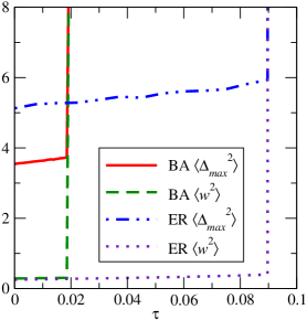
Figure 1: (Color online) The typical behavior of the steady-state average width and the expected extreme as a function of the delay $\tau$ for an ER and a BA network with $N$$=$$1000$ and $\langle k\rangle\approx 6$.

III Extreme Fluctuations

With an understanding of the typical fluctuations of the underlying modes, we may now proceed to consider the extreme fluctuations in a network. Consider the covariance matrix of fluctuations at the nodes (i.e., the steady-state equal-time correlations), $\sigma^{2}_{ij}\equiv\langle\Delta_{i}\Delta_{j}\rangle$, and that of the modes, $\tilde{\sigma}^{2}_{k\ell}\equiv\langle\tilde{h}_{k}\tilde{h}_{\ell}\rangle=\delta_{k\ell}\tilde{\sigma}^{2}_{k}$ (where the single subscript denotes the diagonal elements). The distribution of a single mode follows a zero-mean normal (Gaussian) distribution with a variance given by Eq. (11),

$$\tilde{\sigma}_{k}^{2}=\langle\tilde{h}_{k}^{2}\rangle=D\tau f(\lambda_{k}\tau)\;.$$ (14)

In turn, the fluctuations from the modes translate back to those at the nodes according to $\boldsymbol{\sigma}^{2}=S\tilde{\boldsymbol{\sigma}}^{2}S^{-1}$, where $S$ is an orthogonal matrix with columns composed of the normalized eigenvectors of the network Laplacian (i.e., $\Gamma=S\Lambda S^{-1}$, where $\Lambda$ is a diagonal matrix of the eigenvalues). Since $\tilde{\boldsymbol{\sigma}}^{2}$ is diagonal, this transformation can be written simply as

$$\langle\Delta_{i}^{2}\rangle=\sigma^{2}_{i}=\sum_{k}S_{ik}^{2}\tilde{\sigma}^{2}_{k}\;.$$ (15)

The marginal distributions of the fluctuations at the nodes ($x=\Delta_{i}$) are Gaussian,

$$p_{i}(x)=\frac{1}{\sqrt{2\pi\sigma^{2}_{i}}}e^{-\frac{x^{2}}{2\sigma_{i}^{2}}}$$ (16)

with zero mean and variance $\sigma^{2}_{i}$ [Eq. (15)]. The effects of several delays on the spread of the distributions for a few representative degree classes are shown in Fig. 2.

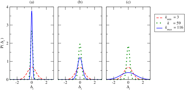
Figure 2: (Color online) Individual node distributions of representative degrees in a BA network with $N$$=$$1000$ and $\langle k\rangle\approx 6$ for fractions $q$ of the critical delay of (a) $q=0$, (b) $q=0.90$, and (c) $q=0.99$ ($q$$=$$\tau/\tau_{c}$).

Each panel shows the distributions for a distinct delay $\tau$, which can be expressed in terms of the fraction relative to the critical delay $q\equiv\tau/\tau_{c}$.

For zero or small delays the size of the fluctuations (the width of the distributions) at a node decreases monotonically with the node’s degree, i.e., the larger the degree the narrower the distribution [Fig. 2(a,b)]. For a sufficiently large delay, however, the trend changes, and the node with the largest degree can exhibit the largest fluctuations [Fig. 2(c)]. This can be understood by noting that in a mean-field sense, the effective coupling at each node is its degree $k_{i}$ [3, 24]. Thus, the fluctuations at each node are approximately proportional to $f(k_{i}\tau)$ (where the scaling function is known exactly [Eq. (11)]), and it is non-monotonic in its argument [5, 7]. This trend is also illustrated in Fig. 3. For zero (or small) delay the average fluctuations at a node decay as $\langle\Delta_{i}^{2}\rangle\sim 1/k_{i}$ [3, 24]. In contrast, the average size of the fluctuations as a function of the degree becomes non-monotonic for large delays [Fig. 3]. The fluctuations at the low-degree nodes remain largely unaffected, while fluctuations at the large-degree nodes increase significantly.

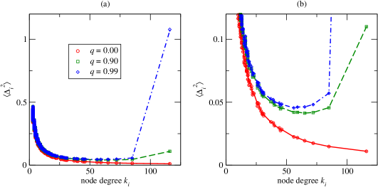
Figure 3: (Color online) (a) Average size of the fluctuations at the nodes as a function of their degree for a BA network with $N$$=$$1000$ and $\langle k\rangle$$\approx$$6$. Open symbols correspond to results based on exact numerical diagonalization of the Laplacian and employing Eqs. (14) and (15). Plus symbols (of matching colors) correspond to the direct numerical integration of the stochastic delay-differential Eq. (5) with $\Delta t$$=$$5\times 10^{-6}$. The connecting lines are the average of the degree class from these numerical integrations. (b) Same data as in (a) but on smaller vertical scales.

For networks with no delays it has been established that the nodes with the smallest degree typically contribute most to the extremes [24, 45], which is still valid in the case of small delays ($\tau/\tau_{c}\ll 1$). For scale-free (SF) networks with power-law degree distributions, such as BA networks [50], the low-degree nodes can still dominate the distribution of extreme fluctuations at higher delays (but $\tau<\tau_{c}$) since they are more numerous, even though the typical fluctuations for the highest degree node are larger than for a single low degree node. So long as the highest degree node’s fluctuations do not dominate the extremes of the network, the large set of lowest degree nodes will lead to the familiar FTG distribution for the network’s extremes [Fig. 4(a)]. Note that the approach to the FTG limit distribution can be very slow due to the slowly vanishing corrections for Gaussian-like individual variables [64]. Further, for larger delays, the convergence to the FTG density may not be monotonic due to the larger effect of the largest-degree node for small system sizes [Fig. 4(b)].

Note that the largest eigenvalue of the network Laplacian varies among individual realizations of a random network ensemble. Therefore, to simulate “similar” synchronization dynamics in a network random ensemble (e.g., of $1000$ networks of size $N$), we kept $q$, the fraction of the delay relative to the critical delay, fixed in the individual network realizations (i.e., an individual network realization $\ell$ has a delay $\tau^{(\ell)}=q\tau_{c}^{(\ell)}$). Further, also note that the largest eigenvalue of the Laplacian diverges with the largest degree in a graph [67, 68], hence it diverges with the network size $N$ in complex networks, e.g., in a power-law fashion for SF networks [69, 70], and logarithmically for ER and SW networks [5, 7].

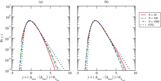
Figure 4: (Color online) Finite-size behavior of the distribution of the extreme fluctuations for BA networks with $\langle k\rangle$$\approx$$6$ and relative delays (a) $q$$=$$0.5$ and (b) $q$$=$$0.9$ obtained by numerically integrating Eq. (5) using $\Delta t$$=$$5\times 10^{-6}$. The dotted curves in both panels correspond to the scaled FTG density, Eq. (4).

We found similar behavior for other prototypical networks [SW, ER and BA], namely for $\tau$$<$$\tau_{c}$ the scaled distributions of the extreme fluctuations converge to the FTG density [Fig. 5].

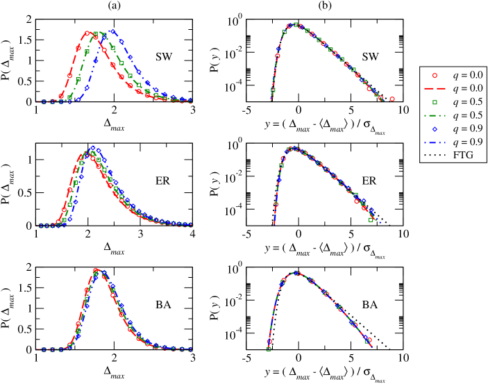
Figure 5: (Color online) (a) Extreme fluctuation distributions and (b) rescaling of the same for several delays for SW, ER, and BA networks with $N$$=$$1000$ and $\langle k\rangle$$\approx$$6$. The various curves correspond to the same delay fraction $q$ for both (a) and (b). Lines are predictions based on exact numerical diagonalization and employing Eqs. (14), (15), and (19). Symbols correspond to the numerical integration of the stochastic delay-differential equations Eq. (5) with $\Delta t=5\times 10^{-6}$. The dotted curves in all panels correspond to the scaled FTG density, Eq. (4).

Also, our results for ER and BA networks indicate that the extreme fluctuations $\langle\Delta_{\max}\rangle$ asymptotically approach a logarithmic scaling with the system size $N$ [Fig. 6], consistent with being governed by the FTG density.

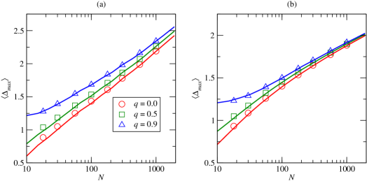
Figure 6: (Color online) Scaling of the expected maximum fluctuations $\langle\Delta_{\max}\rangle$ with system size $N$ for ensembles of (a) ER and (b) BA networks ($1000$ realizations). Open symbols correspond to simulating the stochastic delay-differential equations Eq. (5) with $\Delta t$$=$$0.001$) Solid curves show predictions based on exact numerical diagonalization and employing Eqs. (14), (15), and (19).

To provide further insights to the source of the extreme fluctuations in BA networks, we also analyzed the distribution of the extremes within each degree class. We have already seen that the average size of fluctuations are the largest for small degrees, except for near-critical delays [Fig. 3]. When the delay approaches the critical value for a given graph, the average size of the fluctuations becomes a non-monotonic function of the degree (in a mean-field sense, this behavior is naturally related to U-shape scaling behavior of the fluctuations with the effective coupling [5, 7]). In fact, there is a regime where the fluctuations at the largest degree node are finite and are the largest in the network. In parallel with the above observation, sufficiently below the critical delay of a given graph, the extreme fluctuations will almost always originate in the class of nodes with the smallest degree: not only the average size of the fluctuations is the largest here, but also this degree class has the largest population (as given by the degree distribution). In this regime, it is thus expected that the global distribution of the extreme fluctuations will essentially overlap with the extremes within the class of the minimum degree. Our simulations confirm this in Fig. 7(a) and (b). Further, as the delay approaches its critical value in the given graph, the (single) node with the largest degree will often give rise to the largest fluctuations in the network. This is demonstrated in Fig. 7(c), showing that the tail of the global extremes coincides with the (Gaussian) fluctuations at a (single) node with the largest degree.

When the delay in a given network is not too close to the critical delay, one can assume that the fluctuations at the nodes decouple. This assumption works fairly well for complex networks with no delays [54, 55, 45]. (Note that such assumption is ill-fated for low-dimensional spatial graphs where a large correlation length governs the scaling.) Now we test this hypothesis for complex networks with delays, and predict the extreme limit distribution of the fluctuations. The cumulative distribution of the fluctuations at a particular node $i$ (with $x=\Delta_{i}$) can be expressed in terms of the error function,

$$P^{<}_{i}(x)=\int_{-\infty}^{x}dx^{\prime}p_{i}(x^{\prime})=\int_{-\infty}^{x}dx^{\prime}\frac{e^{-x^{\prime 2}/2\sigma_{i}^{2}}}{\sigma_{i}\sqrt{2\pi}}=\frac{1}{2}\left\{1+\frac{2}{\sqrt{\pi}}\int_{0}^{x/\sigma_{i}\sqrt{2}}dte^{-t^{2}}\right\}=\frac{1}{2}\left\{1+{\rm erf}\left(\frac{x}{\sigma_{i}\sqrt{2}}\right)\right\}\;.$$ (17)

Assuming independence of the nodes in determining the extremal fluctuations, the cumulative distribution for the maximum fluctuation during a given snapshot is

$$P^{{}<{}}_{\max}(x)\simeq\prod_{i=1}^{N}P^{{}<{}}_{i}(x).$$ (18)

The corresponding density from Eqs. (17) and (18) is then

$$p_{\max}^{<}(x)=\frac{d}{dx}P^{<}_{\max}(x)\simeq\sum_{i}^{N}p_{i}(x)\prod_{j\neq i}P^{{}<{}}_{j}(x)=\frac{2^{1/2-N}}{\sqrt{\pi}}\sum_{i=1}^{N}\left\{\frac{e^{-x^{2}/2\sigma_{i}^{2}}}{\sigma_{i}}\prod_{j\neq i}\left[1+{\rm erf}\left(\frac{x}{\sigma_{j}\sqrt{2}}\right)\right]\right\}.$$ (19)

The results based on the above approximation (together with those given by the actual numerical simulations) are shown in Fig. 5 for the distribution, and in Fig. 6 for the average of the extremes. Note that the validity of this approximation can break down when the delay is sufficiently close to the critical delay so that fluctuation at the few highest degree nodes can completely dominate the extremes.

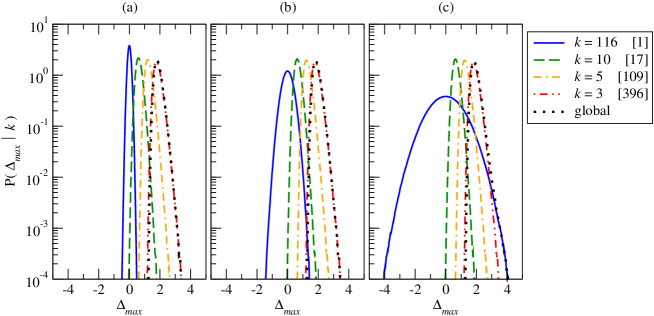
Figure 7: (Color online) Contribution of a few selected degree classes for a BA network (including $k_{\rm min}$$=$$3$ and $k_{\rm max}$$=$$116$) with $N=1000$ and $\langle k\rangle\approx 6$ for (a) $q=0.0$, (b) $q=0.9$ and (c) $q=0.99$. Results are obtained from numerical integration of the stochastic delay-differential equations Eq. (5) with $\Delta t=5\times 10^{-6}$. The numbers in brackets in the legends indicate the number of nodes in the corresponding degree class.

Also, note that the fluctuations of the mode associated with the largest eigenvalue assumes large oscillatory components for $\lambda_{\max}\tau>1/e$ [5, 7]. This manifests with the greatest amplitude at the largest degree node with strong oscillatory components. Once the delay is sufficiently close to the critical delay so that these large-amplitude oscillations dominate the extremes, an additional feature emerges in the distribution of $\Delta_{\max}$. Here, there is a broader non-universal tail, which originates from the finite but very large fluctuations at the node with the largest degree [Fig. 7(c)]. The suppression of the contribution from low degree nodes is compounded if more than one node has the network’s maximum degree. Periodically, when the oscillatory behavior of this node brings it back near the mean $\bar{h}(t)$, the global extremes can still be dominated by the FTG-distributed extremes among the lowest-degree nodes.

IV The Width and the Extremes on Regular Lattices

Finally, it is worthwhile to contrast the steady-state scaling behavior of the extremes and their distributions in complex networks to those on regular lattices. For regular $d$-dimensional lattices the largest eigenvalue of the Laplacian is independent of the system size. Thus, for a fixed delay $\tau$, if the system is synchronizable for a particular system size, it is synchronizable for all system sizes, $\lambda_{\max}\tau<\pi/2$, and the usual $N\to\infty$ thermodynamic limit can be considered with no delay-induced instability. Further, as $N\to\infty$, the arbitrarily small eigenvalues of the Laplacian ($\lambda_{\min}\sim N^{-2/d}$) will dominate the sum in Eq. (12), just like they do in systems with no delay. Hence, one can expect that the scaling of the width, the extremes and their asymptotic limit distribution in the synchronizable regime will be identical to those with no delay, governed by a diverging correlations and long-wavelength modes (associated with the arbitrarily small eigenvalues of the Laplacian). For illustration, we considered one-dimensional lattices (with nearest-neighbor coupling) with delays [Fig. 8]. For completeness, we studied the detailed finite-size behavior of both the steady-state width distribution $P(w^{2})$ and the distribution of the extremes $P(\Delta_{\max})$. The results of the numerical integration of the systems with delays (but within the synchronizable regime, $\lambda_{\max}\tau<\pi/2$) show that the asymptotic limit distributions of the width and the extreme fluctuations approach those of the delay-free systems, the FORWZ distribution [60] and the Airy distribution [57, 58], respectively [Fig. 9].

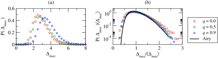
Figure 8: (Color online) (a) Extreme fluctuation distributions and (b) scaled version of the same data for several delays for a regular one-dimensional lattice with $N$$=$$1000$. Symbols are the results found by numerically integrating Eq. (5) using $\Delta t=5\times 10^{-6}$. The solid line corresponds to the predicted asymptotic Airy limit distribution [57, 58].

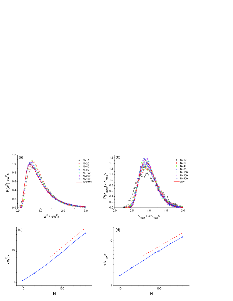
Figure 9: (Color online) (a) Finite-size behavior of the scaled width distribution for one-dimensional lattices for fixed time delay $\tau=0.25$. The solid line corresponds to the predicted asymptotic FORWZ limit distribution [60]. (b) Finite-size behavior of the scaled extreme fluctuation distribution for regular one-dimensional lattices for the same system sizes and delay as in (a). The solid line corresponds to the predicted asymptotic Airy limit distribution [57, 58]. (c) Finite-size behavior of the average width for the same system sizes and delay as in (a). The dashed line is to guide the eyes, corresponding to the asymptotic theoretical prediction, $\langle w^{2}\rangle\sim N$. (d) Finite-size behavior of the extreme fluctuations for the same system sizes and delay as in (b). The dashed line is to guide the eyes, corresponding to the asymptotic theoretical prediction, $\langle\Delta_{\max}\rangle\sim N^{1/2}$.

V Exploring the Effects of Nonlinear Couplings

While in our current work the focus has been to understand the effects of time delays on stochastic systems with liner couplings, we performed some explorations on the nonlinear effects. We considered the stochastic equation

$$\partial_{t}h_{i}(t)=-\sum_{j=1}^{N}C_{ij}(h_{i}-h_{j})+\nu\sum_{j,k=1(j<k)}^{N}C_{ij}C_{ik}(h_{j}-h_{i})(h_{k}-h_{i})+\eta_{i}(t)\;,$$ (20)

where the effects of time delays are captured, as before, by replacing $\{h_{l}(t)\}_{l=1}^{N}$ by $\{h_{l}(t-\tau)\}_{l=1}^{N}$ in the right-hand side of the above stochastic differential equation. Such nonlinear terms can be motivated by, for example, coarse-graining local growth processes in networks [21, 43, 44, 45, 71] (e.g., where only local network-neighborhood minima can progress). Note that in one dimension, the above stochastic equation reduces to

$$\partial_{t}h_{i}(t)=-(2h_{i}-h_{i+1}-h_{i-1})+\nu(h_{i+1}-h_{i})(h_{i-1}-h_{i})+\eta_{i}(t)\;.$$ (21)

The above equation is just a (somewhat unconventional) discretization of the well-known KPZ equation [72, 73],

$$\partial_{t}h(x,t)=\nabla^{2}h-\nu(\nabla h)^{2}+\eta_{i}(t)\;,$$ (22)

which can be easily seen by taking the naive continuum limit in Eq. (21), $h_{i\pm 1}(t)=h(x,t)\pm\partial h/\partial x+\ldots$, and keeping only the leading-order derivatives.

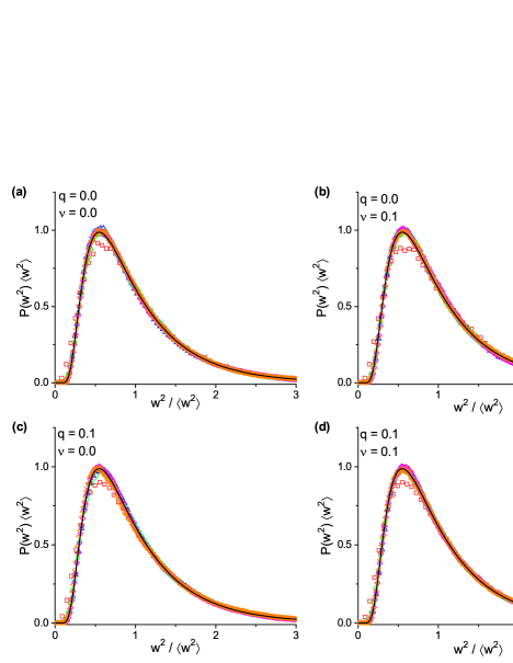
Figure 10: (Color online) Finite-size behavior of the scaled width distribution for one-dimensional lattices with nonlinear coupling $\nu$ [Eq. (21)] and relative time delay $q=\tau/\tau_{\rm c}$. (a) $\nu=0.0$, $q=0.0$; (b) $\nu=0.1$, $q=0.0$; (c) $\nu=0.0$, $q=0.1$; (d) $\nu=0.1$, $q=0.1$. The solid line corresponds to the predicted asymptotic FORWZ limit distribution [60].

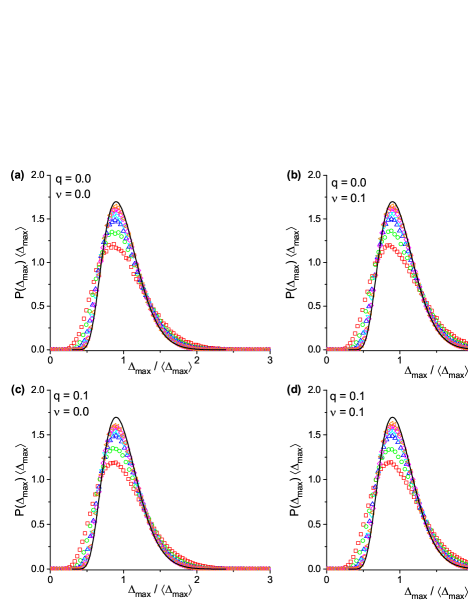
Figure 11: (Color online) Finite-size behavior of the scaled distribution of the extreme fluctuation above the mean for regular one-dimensional lattices with nonlinear coupling $\nu$ [Eq. (21)] and relative time delay $q=\tau/\tau_{\rm c}$. (a) $\nu=0.0$, $q=0.0$; (b) $\nu=0.1$, $q=0.0$; (c) $\nu=0.0$, $q=0.1$; (d) $\nu=0.1$, $q=0.1$. The solid line corresponds to the predicted asymptotic Airy limit distribution [57, 58].

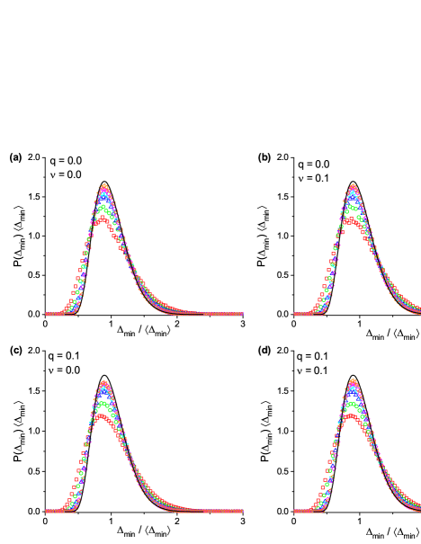
Figure 12: (Color online) Finite-size behavior of the scaled distribution of the extreme fluctuation below the mean for regular one-dimensional lattices with nonlinear coupling $\nu$ [Eq. (21)] and relative time delay $q=\tau/\tau_{\rm c}$. (a) $\nu=0.0$, $q=0.0$; (b) $\nu=0.1$, $q=0.0$; (c) $\nu=0.0$, $q=0.1$; (d) $\nu=0.1$, $q=0.1$. The solid line corresponds to the predicted asymptotic Airy limit distribution [57, 58].

First, we studied one-dimensional regular lattices (with nearest-neighbor connections and periodic boundary conditions). In what follows, we parameterized the delay relative to the critical delay of the linear system for reference, $q\equiv\tau/\tau_{c}$. Numerically integrating the time-discretized version of the stochastic differential equation Eq. (21) (see Supplemental Material for more details), we have found that for sufficiently small values of the nonlinear coupling $\nu$ and time delays, the system reaches a steady state with a finite width for finite systems. The width distribution [Fig. 10] and the distribution of the extremes for both above [$\Delta_{\max}=h_{\max}-\bar{h}$, Fig. 11] and below the mean [$\Delta_{\min}=\bar{h}-h_{\min}$, Fig. 12] approach the FORWZ and the Airy distribution, respectively, similar to the case of pure linear couplings.

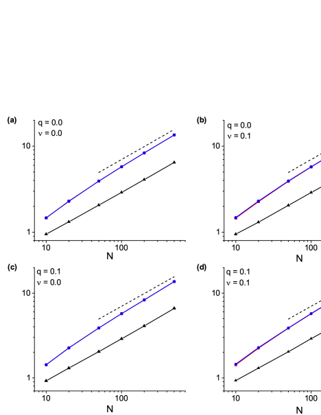
Figure 13: (Color online) Scaling of the average width $w\equiv\sqrt{\langle w^{2}\rangle}$ and the expected extreme fluctuations $\Delta_{\max}$ and $\Delta_{\min}$ (the expected largest fluctuations above and below the mean, respectively) with the system size in regular one-dimensional lattices with nonlinear coupling $\nu$ [Eq. (21)] and relative time delay $q=\tau/\tau_{\rm c}$. The dashed lines are to guide the eyes, corresponding to the scaling $\sim N^{1/2}$. Note the log-log scales. (a) $\nu=0.0$, $q=0.0$; (b) $\nu=0.1$, $q=0.0$; (c) $\nu=0.0$, $q=0.1$; (d) $\nu=0.1$, $q=0.1$.

Further, the average width and the extremes (both above and below the mean height) scale as $N^{1/2}$ with the system size [Fig. 13].

Investigating the behavior of the width for larger values of the nonlinear coupling, it is clear the synchronization profile can diverge (the system becomes unstable), even for zero time delay (see Supplemental Material). We checked and tested that this instability is not an artifact of the finite time difference $\Delta t$, but rather it is the result of the non-linear term on discrete lattices in Eq. (21). Indeed, it has been well documented [58, 75, 76, 77, 78, 79] that even conventional lattice discretization schemes of the KPZ nonlinearity can give rise to instability in a noisy environment (even though its spatial continuum limit is stable and the nonlinear term, in fact, exactly cancels by symmetry in the stationary state [72, 73, 74]). Our observed behavior, induced by the nonlinear KPZ term in Eq. (21), is just another example for such instability, intrinsic on discrete structures, such as lattices.

In networks, we found similar behavior. For example, in ER networks, we found that the nonlinear term in Eq. (20) gives rise to a diverging width even for our smallest value of the nonlinear coupling strength $\nu$, even in the absence of time delays (see Supplemental Material). We again checked and confirmed that the lack of stability in the presence of nonlinear couplings is not the result of insufficient time discretization of the stochastic differential equation (20) (see Supplemental Material). For small values of the nonlinear coupling $\nu$, there exist, however, a long “quasi-stationary” period before fluctuations begin to diverge, where we analyzed the statistical properties of the extremes. We have found that during this quasi-stationary period, the scaled distributions of the extremes are reasonably well-described by the FTG limit densities [Fig. 14].

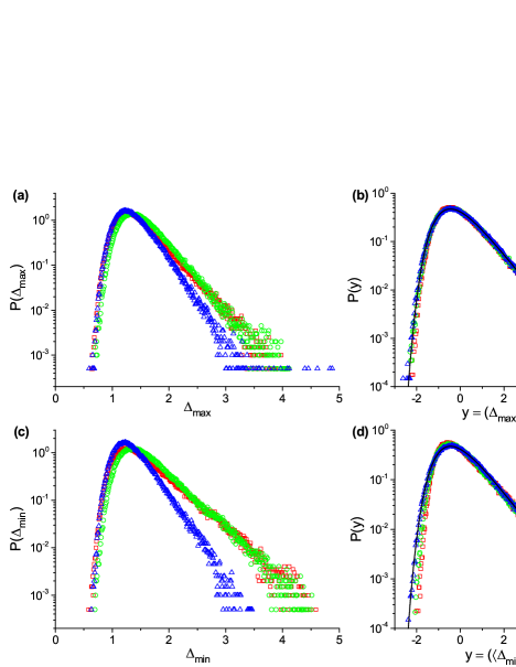
Figure 14: (Color online) Extreme fluctuation distribution (in the quasi-stationary period) in ER networks with $N=100$, $\langle k\rangle\approx 6$, nonlinear coupling $\nu=0.1$ [Eq. (20)], and various relative time delays $q=\tau/\tau_{\rm c}$. (a) Distributions of the extreme fluctuations above the mean, $\Delta_{\max}=h_{\max}-\bar{h}$; (b) Scaled distributions of the extreme fluctuations above the mean (with zero mean and unit variance); (c) Distributions of the extreme fluctuations below the mean, $\Delta_{\min}=\bar{h}-h_{\min}$; (d) Scaled distributions of the extreme fluctuations below the mean (with zero mean and unit variance). The solid line in (b) and (d) corresponds to the FTG limit distribution [Eq. (4)].

For SW networks, while the fluctuations (and the width) are smaller than those than on one-dimensional lattices (at least during the quasi-stationary period), the synchronization landscape eventually becomes unstable for sufficiently strong nonlinear coupling, with or without delays (see Supplemental Material). We also observe that the average width in the quasi-stationary period is decreasing with increasing average degree $\langle k\rangle$, but at the same time, the duration of the quasi-stationary period is decreasing with increasing $\langle k\rangle$ (see Supplementary Material). Nevertheless, in the stationary (or quasi-stationary) state, the scaled distributions of the extremes are well-described by the FTG limit densities [Fig. 15].

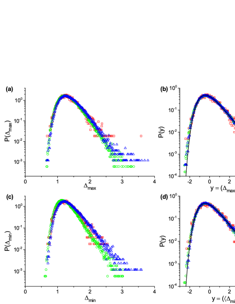
Figure 15: (Color online) Extreme fluctuation distribution (in the quasi-stationary period) in SW networks with $N=100$, $\langle k\rangle\approx 6$, nonlinear coupling $\nu=0.1$ [Eq. (20)], and various relative time delays $q=\tau/\tau_{\rm c}$. (a) Distributions of the extreme fluctuations above the mean, $\Delta_{\max}=h_{\max}-\bar{h}$; (b) Scaled distributions of the extreme fluctuations above the mean (with zero mean and unit variance); (c) Distributions of the extreme fluctuations below the mean, $\Delta_{\min}=\bar{h}-h_{\min}$; (d) Scaled distributions of the extreme fluctuations below the mean (with zero mean and unit variance). The solid line in (b) and (d) corresponds to the FTG limit distribution [Eq. (4)].

It is clear that we have only begun to scratch the surface of the complexity of the behavior as a result of nonlinear couplings in the stochastic delay differential equations in networks. Among the important questions that one shall investigate are the effects of the strength of nonlinear coupling, time delay, and network size on the length of the quasi-stationary period. It is also clear from our explorations that uncontrolled expansions of local growth processes (i.e., naive coarse graining) may result in nonlinear terms in the resulting stochastic differential equations (with or without delays) which give rise to instability and diverging width in the synchronization landscape. This instability is “real” (i.e., not an artifact of time discretization) as far as the numerical integration of the stochastic differential equation is concerned, but may not be present in the actual physical systems with the original microscopic rules [21, 43, 44, 45].

VI Summary

We have demonstrated that the extreme fluctuations in stochastic coordination or synchronization problems with time delays (with short-tailed node-level noise and within the linearized approximation) can fall in two main classes. In complex or random networks (e.g., ER, SF, or SW graphs), if the system is sufficiently large but synchronizable ($\lambda_{\max}\tau<\pi/2$), the distribution of the extremes is governed by the FTG distribution, while the average size of the largest fluctuations does not grow faster than logarithmic. This type of scaling behavior can be understood as the fluctuations at the nodes are only weakly correlated, hence traditional extreme-value limit theorems apply. In contrast, in spatial graphs, fluctuations at the nodes are strongly correlated. As demonstrated on one-dimensional regular rings, the distribution of the extremes approaches the Airy limit distribution, while the average size of the largest fluctuations will scale as the width itself, e.g., as a power law in one dimension.

Finally, we have performed some explorations on the effects on nonlinear couplings in the stochastic delay differential equations in networks. Our results indicate the generalized KPZ nonlinearity in discrete structures (networks) can ultimately give rise to instability. Even in that case, however, during a quasi-stationary period (before the width diverges), the statistics of the extreme fluctuations are well-described by the Airy and FTG densities, in one dimension and in random ER/SW graphs, respectively. Clearly, future investigations are needed to precisely characterize the stability conditions in the presence of nonlinear couplings in networks with (and without) time delays.

Supplemental Material

In this Supplemental Material, we provide some additional results (figures) obtained by the numerical integration of the stochastic delay differential equation

$$\partial_{t}h_{i}(t)=-\sum_{j=1}^{N}C_{ij}(h_{i}-h_{j})+\nu\sum_{j,k=1(j<k)}^{N}C_{ij}C_{ik}(h_{j}-h_{i})(h_{k}-h_{i})+\eta_{i}(t)\;,$$ (S1)

discussed in Sec. V. in the main text. The effects of time delays are captured by replacing $\{h_{l}(t)\}_{l=1}^{N}$ by $\{h_{l}(t-\tau)\}_{l=1}^{N}$ in the right-hand side of Eq. (S1). In the above continuous-time stochastic differential equation, the noise $\eta_{i}(t)$ is Gaussian with zero mean and correlations $\langle\eta_{i}(t)\eta_{j}(t^{\prime})\rangle=2D\delta_{ij}\delta(t-t^{\prime})\rangle$. In the present work, we considered unweighted graphs, i.e., $C_{ij}$ is just the adjacency matrix. The time-discretized version of Eq. (S1) becomes [1-5]

$$h_{i}(t+\Delta t)-h_{i}(t)=-\Delta t\sum_{j=1}^{N}C_{ij}(h_{i}-h_{j})+\Delta t\,\nu\sum_{j,k=1(j<k)}^{N}C_{ij}C_{ik}(h_{j}-h_{i})(h_{k}-h_{i})+\hat{\eta}_{i}(t)\sqrt{2D\Delta t}\;,$$ (S2)

where $\hat{\eta}_{i}(t)$ are independent and identically distributed random variables for all $i$ and $t$ with Gaussian distribution of zero mean and unit variance. In our simulations, without loss of generality, we set $D$$=$$1$. For example, in one dimension, with nearest neighbor couplings and periodic boundary conditions, the above equation becomes

$$h_{i}(t+\Delta t)-h_{i}(t)=-\Delta t(2h_{i}-h_{i+1}-h_{i-1})+\Delta t\,\nu(h_{i+1}-h_{i})(h_{i-1}-h_{i})+\hat{\eta}_{i}(t)\sqrt{2D\Delta t}\;.$$ (S3)

Employing Eqs. (S2) and (S3), we explore and display the width of the synchronization landscape as a function of time for a one-dimensional lattice (with nearest-neighbor coupling and periodic boundary conditions) [Fig. S1], ER graphs [Fig. S4], and SW networks [Figs. S7, S8]. We also demonstrate that the instability observed in the resulting stochastic landscapes is not the result of insufficient time discretization in the numerical integration scheme, but rather, it is intrinsic to the generalized KPZ coupling on discrete structures (such as lattices or networks) for sufficiently strong nonlinear coupling and/or large time delays. To that end, we show the average time to desynchronization (the onset of instability) as a function of $\Delta t$ used in the above numerical integration scheme for a one-dimensional lattice [Fig. S2], ER networks [Fig. S5], and SW networks [Fig. S9]. Finally, we show the average time to desynchronization as a function of the nonlinear coupling $\nu$ and relative time delay $q=\tau/\tau_{c}$ in a one-dimensional lattice [Fig. S3], ER networks [Fig. S6], and SW networks [Fig. S10]. Our results for SW networks [Figs. S7 and S8] also suggest that while increasing connectivity (average degree $\langle k\rangle$) reduces the width in the quasi-stationary state, the quasi-stationary period is becoming shorter, i.e., the system is more prone to instability.

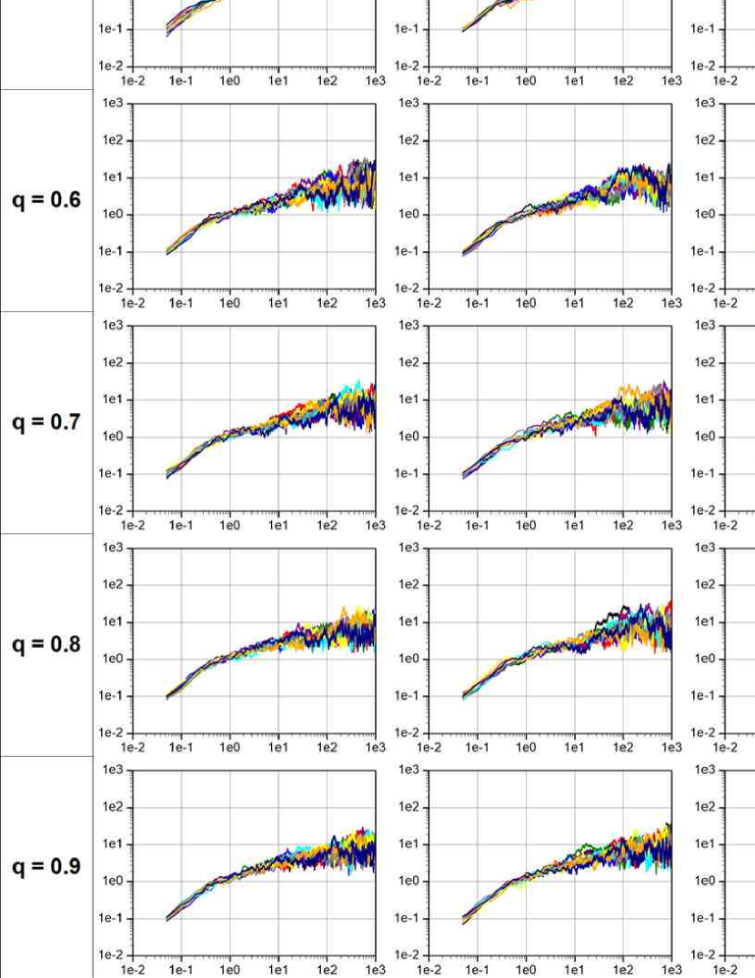
Figure S1: Graphical table of the evolution of the width over time, in a one-dimensional regular lattice (with periodic boundary conditions) with $N$$=$$100$ for KPZ-like coupling [Eq. (S3)]. Each tile shows the width $\langle w^{2}\rangle$ as a function of time, using identical scales in each tile. Data was obtained by numerically integrating Eq. (S3) with $\Delta t=10^{-3}$. Colors represent $10$ distinct realizations of noise. Each row corresponds to the indicated value of time delay $q=\tau/\tau_{c}$, and each column corresponds to the indicated nonlinear coupling strength $\nu$. A high-resolution version of this figure is provided separately in TIFF format among the Supplemental Materials (W2vsTimeMap_Ring.tif).

Figure S2: Average time to desynchronization for KPZ-like coupling [Eq. (S3)] at various $\Delta t$ time steps of integration on a one-dimensional regular lattice (with periodic boundary conditions) with $N$$=$$100$, $\nu=0.8$, $q=0.8$. Error bars represent standard deviation, sampled over $100$ realizations.

Figure S3: Time to reach desynchronization for KPZ-like coupling [Eq. (S3)], as a function of the delay $q=\tau/\tau_{c}$ and nonlinear coupling strength $\nu$, on a one-dimensional regular lattice (with periodic boundary conditions) with $N$$=$$100$. Data was obtained by numerically integrating Eq. (S3) with $\Delta t=10^{-3}$.

Figure S4: Graphical table of the evolution of the width over time, in ER networks with $N$$=$$100$ and $\langle k\rangle\approx 6$ using generalized KPZ coupling [Eq. (S2)]. Each tile shows the width $\langle w^{2}\rangle$ as a function of time, using identical scales in each tile. Data was obtained by numerically integrating Eq. (S2) with $\Delta t=10^{-4}$. Colors represent $10$ distinct realizations of noise. Each row corresponds to the indicated value of time delay $q=\tau/\tau_{c}$, and each column corresponds to the indicated nonlinear coupling strength $\nu$. A high-resolution version of this figure is provided separately in TIFF format among the Supplemental Materials (W2vsTimeMapER_k6.tif).

Figure S5: Average time to desynchronization for generalized KPZ coupling [Eq. (S2)] at various $\Delta t$ time steps of integration in a ER network with $N$$=$$100$, $\langle k\rangle\approx 6$, $\nu=0.2$, $q=0.2$. Error bars represent standard deviation, sampled over $100$ realizations.

Figure S6: Time to reach desynchronization using generalized KPZ coupling [Eq. (S2)], as a function of the delay $q=\tau/\tau_{c}$ and nonlinear coupling strength $\nu$, for an ER network with $N$$=$$100$ and $\langle k\rangle\approx 6$. Data was obtained by numerically integrating Eq. (S2) with $\Delta t=10^{-3}$.

Figure S7: Graphical table of the evolution of the width over time, in SW networks with $N$$=$$100$ and $\langle k\rangle\approx 3$, using generalized KPZ coupling [Eq. (S2)]. Each tile shows the width $\langle w^{2}\rangle$ as a function of time, using identical scales in each tile. Data was obtained by numerically integrating Eq. (S2) with $\Delta t=10^{-3}$. Colors represent $10$ distinct realizations of noise. Each row corresponds to the indicated value of time delay $q=\tau/\tau_{c}$, and each column corresponds to the indicated nonlinear coupling strength $\nu$. A high-resolution version of this figure is provided separately in TIFF format among the Supplemental Materials (W2vsTimeMapSW_k3.tif).

Figure S8: Graphical table of the evolution of the width over time, in SW networks with $N$$=$$100$ and $\langle k\rangle\approx 6$, using generalized KPZ coupling [Eq. (S2)]. Each tile shows the width $\langle w^{2}\rangle$ as a function of time, using identical scales in each tile. Data was obtained by numerically integrating Eq. (S2) with $\Delta t=10^{-3}$. Colors represent $10$ distinct realizations of noise. Each row corresponds to the indicated value of time delay $q=\tau/\tau_{c}$, and each column corresponds to the indicated nonlinear coupling strength $\nu$. A high-resolution version of this figure is provided separately in TIFF format among the Supplemental Materials (W2vsTimeMapSW_k6.tif).

Figure S9: Average time to desynchronization for generalized KPZ coupling [Eq. (S2)] at various $\Delta t$ time steps of integration in a SW network with $N$$=$$100$, $\langle k\rangle\approx 6$, $\nu=0.2$, $q=0.2$. Error bars represent standard deviation, sampled over $100$ realizations.

Figure S10: Time to reach desynchronization using generalized KPZ coupling [Eq. (S2)], as a function of the delay $q=\tau/\tau_{c}$ and nonlinear coupling strength $\nu$, for a SW network with $N$$=$$100$ and $\langle k\rangle\approx 6$. Data was obtained by numerically integrating Eq. (S2) with $\Delta t=10^{-3}$.

[1] C.W. Gardiner, Handbook of Stochastic Methods, 2nd ed. (Springer-Verlag, New York, 1985).

[2] A.-L. Barabási and H.E. Stanley, Fractal Concepts in Surface Growth (Cambridge University Press, Cambridge, 1995).

[3] C. Dasgupta, J.M. Kim, M. Dutta, and S. Das Sarma, Phys. Rev. E 55, 2235 (1997).

[4] C.-H. Lam and F.G. Shin, Phys. Rev. E 58, 5592 (1998).

[5] S.N. Majumdar and A. Comtet, J. Stat. Phys. 119, 777 (2005).

References

- [1] R. Olfati-Saber, J.A. Fax, and R.M. Murray, Proc. IEEE 95, 215 (2007).
- [2] A. Arenas et al., Phys. Rep. 469, 93 (2008).
- [3] G. Korniss, R. Huang, S. Sreenivasan, and B.K. Szymanski, in Handbook of Optimization in Complex Networks: Communication and Social Networks, edited by M.T. Thai and P. Pardalos, Springer Optimization and Its Applications Vol. 58, (Springer, New York, 2012) pp. 61-96.
- [4] R. Sipahi et al, IEEE Contr. Sys. 31, 38 (2011).
- [5] D. Hunt, G. Korniss, and B.K. Szymanski, Phys. Rev. Lett. 105, 068701 (2010).
- [6] D. Hunt, G. Korniss, and B.K. Szymanski, Phys. Lett. A 375, 880 (2011).
- [7] D. Hunt, B.K. Szymanski, and G. Korniss, Phys. Rev. E 86, 056114 (2012).
- [8] S. Hod, Phys. Rev. Lett. 105, 208701 (2010).
- [9] Q. Wang, Z. Duan, M. Perc, and G. Chen, Europhys. Lett. 83, 50008 (2008).
- [10] Q. Wang, M. Perc, Z. Duan, and G. Chen, Phys. Rev. E 80, 026206 (2009).
- [11] Q. Wang, G. Chen, and M. Perc, PLoS One 6, e15851 (2011).
- [12] M. Kalecki, Econometrica 3, 327 (1935).
- [13] R. Frisch and H. Holme, Econometrica 3, 225 (1935).
- [14] U. Küchler and B. Mensch, Stoch. and Stoch. Rep. 40, 23 (1992).
- [15] T. Ohira and T. Yamane, Phys. Rev. E. 61, 1247 (2000).
- [16] T. D. Frank and P.J. Beek, Phys. Rev. E. 64, 021917 (2001).
- [17] T. Hogg and B.A. Huberman, IEEE Trans. on Sys., Man, and Cybernetics 21, 1325 (1991).
- [18] M.G. Earl and S.H. Strogatz, Phys. Rev. E 67, 036204 (2003).
- [19] M. Barahona and L.M. Pecora, Phys. Rev. Lett. 89, 054101 (2002).
- [20] T. Nishikawa, A.E. Motter, Y.-C. Lai, and F.C. Hoppensteadt, Phys. Rev. Lett. 91, 014101 (2003).
- [21] C.E. La Rocca, L.A. Braunstein, and P.A. Macri, Phys. Rev. E 77, 046120 (2008).
- [22] C.E. La Rocca, L.A. Braunstein, and P.A. Macri, Phys. Rev. E 80, 026111 (2009).
- [23] C. Zhou, A.E. Motter, and J. Kurths, Phys. Rev. Lett. 96, 034101 (2006).
- [24] G. Korniss, Phys. Rev. E 75, 051121 (2007).
- [25] W.-X. Wang, L. Huang, Y.-C. Lai, and G.-R. Chen, Chaos 19, 013134 (2009).
- [26] S. Saavedra, K. Hagerty, and B. Uzzi, Proc. Natl. Acad. Sci. U.S.A. 108, 5296 (2011).
- [27] H. M. Smith, Science 82, 151 (1935).
- [28] C. G. Reynolds Computer Graphics 21, 25–34 (1987).
- [29] F. Cucker and S. Smale, IEEE Trans. Automat. Contr. 52, 852 (2007).
- [30] T. Vicsek, A. Czirók, E. Ben-Jacob, I. Cohen, and O. Shochet, Phys. Rev. Lett. 75, 1226 (1995).
- [31] G.E. Hutchinson, Ann. N.Y. Acad. Sci. 50, 221 (1948).
- [32] R.M. May, Ecology 54, 315–325 (1973).
- [33] S. Ruan, in Delay Differential Equations and Applications, edited by O. Arino, M.L. Hbid, and E.A. Dads, NATO Science Series II: Mathematics, Physics and Chemistry, Vol. 205 (Springer, Berlin, 2006) pp. 477–517.
- [34] J.G. Milton, J.L. Cabrera, and T. Ohira, Europhys. Lett. 83, 48001 (2008).
- [35] J. Milton, J.L. Townsend, M.A. King, and T. Ohira, Phil. Trans. R. Soc. A 367, 1181 (2009).
- [36] J.L. Cabrera and J.G. Milton, Phys. Rev. Lett. 89, 158702 (2002).
- [37] J.L. Cabrera, C. Luciani, and J. Milton, Cond. Matt. Phys. 9, 373 (2006).
- [38] E. Izhikevich, SIAM Rev. 43, 315 (2001).
- [39] R. Johari and D. Kim Hong Tan, IEEE/ACM Trans. Networking 9, 818 (2001).
- [40] R. Olfati-Saber and R.M. Murray, IEEE Trans. Automat. Contr. 49, 1520 (2004).
-
[41]
T.J. Ott,
“On the Ornstein-Uhlenbeck process with delayed feedback,”
http://www.teunisott.com/Papers/TCP_Paradigm/Del_O_U.pdf (2006), Date Last Accessed 06/05/2015. - [42] G. Korniss, M.A. Novotny, H. Guclu, Z. Toroczkai, and P.A. Rikvold, Science 299, 677 (2003).
- [43] G. Korniss, Z. Toroczkai, M.A. Novotny, and P.A. Rikvold, Phys. Rev. Lett. 84, 1351 (2000).
- [44] H. Guclu, G. Korniss, M.A. Novotny, Z. Toroczkai, and Z. Rácz, Phys. Rev. E 73, 066115 (2006).
- [45] H. Guclu, G. Korniss, and Z. Toroczkai, Chaos 17 026104 (2007).
- [46] G. Orosz and G. Stepan, Proc. R. Soc. A 462, 2643 (2006).
- [47] G. Orosz, R.E. Wilson, and G. Stepan, Phil. Trans. R. Soc. A 368, 4455 (2010).
- [48] J.A. Fax and R.M. Murray, IEEE Trans. Automat. Contr. 49, 1465 (2004).
- [49] D.J. Watts and S.H. Strogatz, Nature 393, 440 (1998).
- [50] A.-L. Barabási and R. Albert, Science 286, 509 (1999).
- [51] R. Albert and A.-L. Barabási, Rev. Mod. Phys. 74, 47 (2002).
- [52] S.N. Dorogovtsev and J.F.F. Mendes, Adv. in Phys. 51, 1079 (2002).
- [53] P. Erdős and A. Rényi, Publ. Math. Inst. Hung. Acad. Sci. 5 17 (1960).
- [54] H. Guclu and G. Korniss, Phys. Rev. E 69, 065104(R) (2004).
- [55] H. Guclu and G. Korniss, Fluct. Noise Lett. 5, L43 (2005).
- [56] Y.-Z. Chen, Z.-G. Huang, and Y.-C. Lai, Sci. Rep. 4, 6121 (2014).
- [57] S.N. Majumdar and A. Comtet, Phys. Rev. Lett. 92, 225501 (2004).
- [58] S.N. Majumdar and A. Comtet, J. Stat. Phys. 119, 777 (2005).
- [59] S. Raychaudhuri, M. Cranston, C. Przybyla, and Y. Shapir, Phys. Rev. Lett. 87, 136101 (2001).
- [60] G. Foltin, K. Oerding, Z. Racz, R. L. Workman, and R. K. P. Zia, Phys. Rev. E 50, R639 (1994).
- [61] R.A. Fisher and L.H.C. Tippett, Proc. Camb. Philos. Soc. 24, 180–191 (1928).
- [62] E.J. Gumbel, Statistics of Extremes, (New York, Columbia University Press, 1958).
- [63] Extreme Value Theory and Applications, eds. J. Galambos, J. Lechner, and E. Simin, (Kluwer Academic Publishers, Dordrecht 1994).
- [64] For example, for eponential-like asymptotic tail behavior, , and [61, 62, 63].
- [65] L. O’Malley, G. Korniss, and T. Caraco, Bull. Math. Biol. 71, 1160 (2009).
- [66] N.D. Hayes, J. London Math. Soc. s1-25, 226 (1950).
- [67] M. Fiedler, Czech. Math. J. 23, 298 (1973).
- [68] W.N. Anderson and T.D. Morley, Lin. Multilin. Algebra 18, 141 (1985).
- [69] M. Boguña, R. Pastor-Satorras, and A. Vespignani, Eur. Phys. J. B 38, 205 (2004).
- [70] M. Catanzaro, M. Boguña, and R. Pastor-Satorras, Phys. Rev. E 71, 027103 (2005).
- [71] H. Guclu, G. Korniss, C.J. Olson Reichhardt, C. Reichhardt, and Z. Toroczkai, unpublished (2008).
- [72] M. Kardar, G. Parisi, and Y.-C. Zhang, Phys. Rev. Lett. 56, 889 (1986).
- [73] A.-L. Barabási and H.E. Stanley, Fractal Concepts in Surface Growth (Cambridge University Press, Cambridge, 1995).
- [74] S.F. Edwards and D.R. Wilkinson, Proc. R. Soc. London, Ser A 381, 17 (1982).
- [75] C. Dasgupta, S. Das Sarma, and J.M. Kim, Phys. Rev. E 54, R4552(R) (1996).
- [76] C. Dasgupta, J.M. Kim, M. Dutta, and S. Das Sarma, Phys. Rev. E 55, 2235 (1997).
- [77] T.J. Newman and A.J. Bray, J. Phys. A: Math. Gen. 29, 7917 (1996).
- [78] C.-H. Lam and F.G. Shin, Phys. Rev. E 57, 6506 (1998).
- [79] C.-H. Lam and F.G. Shin, Phys. Rev. E 58, 5592 (1998).