Detection of a Type IIn Supernova in Optical Follow-up Observations
of IceCube Neutrino Events

Abstract

The IceCube neutrino observatory pursues a follow-up program selecting interesting neutrino events in real-time and issuing alerts for electromagnetic follow-up observations. In March 2012, the most significant neutrino alert during the first three years of operation was issued by IceCube. In the follow-up observations performed by the Palomar Transient Factory (PTF), a Type IIn supernova (SN) PTF12csy was found $0.2\text{\,}\mathrm{\SIUnitSymbolDegree}$ away from the neutrino alert direction, with an error radius of $0.54\text{\,}\mathrm{\SIUnitSymbolDegree}$. It has a redshift of $z=0.0684$, corresponding to a luminosity distance of about $300\text{\,}\mathrm{M}\mathrm{p}\mathrm{c}$ and the Pan-STARRS1 survey shows that its explosion time was at least 158 days (in host galaxy rest frame) before the neutrino alert, so that a causal connection is unlikely. The a posteriori significance of the chance detection of both the neutrinos and the SN at any epoch is within IceCube’s 2011/12 data acquisition season. Also, a complementary neutrino analysis reveals no long-term signal over the course of one year. Therefore, we consider the SN detection coincidental and the neutrinos uncorrelated to the SN. However, the SN is unusual and interesting by itself: It is luminous and energetic, bearing strong resemblance to the SN IIn 2010jl, and shows signs of interaction of the SN ejecta with a dense circumstellar medium. High-energy neutrino emission is expected in models of diffusive shock acceleration, but at a low, non-detectable level for this specific SN. In this paper, we describe the SN PTF12csy and present both the neutrino and electromagnetic data, as well as their analysis.

1. INTRODUCTION

IceCube is a cubic-kilometer-sized neutrino detector installed in the ice at the geographic South Pole between depths of 1450 m and 2450 m (Achterberg et al., 2006). It consists of an array of $5160$ photon sensors, called Digital Optical Modules (DOMs), attached to 86 cables, called strings. Detector construction started in 2005 and finished in December 2010. Neutrino observation relies on the optical detection of Cherenkov radiation emitted by secondary particles produced in neutrino interactions in ice or bedrock near IceCube. Due to the small neutrino interaction cross-section, the kilometer-scale detector has an effective area of only $0.2510\text{\,}\mathrm{m}^{2}$ for muon neutrinos of $110\text{\,}\mathrm{T}\mathrm{e}\mathrm{V}$ energy (Aartsen et al., 2014b). As part of the Optical Follow-Up (OFU) program, the IceCube neutrino observatory records high-energy ($\sim$100\text{\,}\mathrm{G}\mathrm{e}\mathrm{V}$\dots$1\text{\,}\mathrm{P}\mathrm{e}\mathrm{V}$$) neutrino events at a rate of about $3\text{\,}\mathrm{m}\mathrm{H}\mathrm{z}$, about 250 per day. Those events are mostly ($\sim 90\%$) cosmic-ray induced neutrinos from the atmosphere, referred to as atmospheric neutrinos, with about a 10% contamination of cosmic-ray induced atmospheric muons.

Routine neutrino analyses in IceCube, which are referred to as offline analyses, are performed after a certain amount of data, e.g. one or several years, has been collected. They benefit from events being put through computationally expensive reconstructions, as well as information on detector performance that become available only days or weeks after data acquisition. In contrast, neutrino analyses running online will not have access to such information, but have the advantage of being near real-time—results are available with a latency of $\sim$3\text{\,}\mathrm{m}\mathrm{i}\mathrm{n}$$. With such a short latency neutrino analysis, multi-wavelength follow-up observations can be triggered by neutrino events. These follow-up data have the potential to reveal the electromagnetic counterpart of a transient neutrino source, which might otherwise be missed and thus be unavailable for further observations. In addition, the coincident detection of neutrino and electromagnetic emission can be statistically more significant and provide more information about the physics of the source than the neutrino detection alone. Another advantage of an online analysis is the prompt availability of the reconstructed neutrino dataset and thus the possibility of fast response analyses. Thus, IceCube’s online neutrino analysis efforts have also enabled fast $\gamma$-ray burst (GRB) searches like the one following GRB 130427A, published in a GCN Circular (Blaufuss, 2013).

The online search for short transient neutrino sources (order of $\leq$100\text{\,}\mathrm{s}$$) is mostly motivated by models of neutrinos from long duration GRBs (Waxman & Bahcall, 1997; Murase, 2008; Murase et al., 2006; Becker et al., 2006) and from choked jet supernovae (SNe) (Razzaque et al., 2004; Ando & Beacom, 2005). The two source classes are related: Both are thought to host a jet, which is highly relativistic in case of long GRBs, but only mildly relativistic in case of choked jet SNe. Long GRB progenitors are conceived to be Wolf-Rayet stars that have lost their outer hydrogen and helium envelope (Meszaros, 2006), while choked jet SNe can still have those outer layers (Ando & Beacom, 2005) which are important for efficient high-energy (HE) neutrino production. The choked jet is more baryon-rich and has a much lower Lorentz factor $\Gamma\approx 3$ than the GRB jet with $\Gamma\gtrsim 100$. It cannot penetrate the stellar envelope and remains optically thick, making it invisible in $\gamma$-rays. The neutrinos produced at $\mathrm{T}\mathrm{e}\mathrm{V}$ energies can escape nevertheless and may trigger the discovery of the SN in other channels. In particular, for a bright nearby SN, a neutrino detection would enable the acquisition of optical data during the rise of the light curve, strengthening the time correlation between the neutrino burst and the optical supernova via the improved estimate of the explosion time (Cowen et al., 2010). Mildly relativistic jets may occur in a much larger fraction of core-collapse SNe than highly relativistic jets, i.e. GRBs (Razzaque et al., 2004; Ando & Beacom, 2005).

Detections of neutrinos from GRBs and choked jet SNe would be a remarkable discovery and could provide important insight into the supernova-GRB connection and the underlying jet physics (Ando & Beacom, 2005). Both sources are expected to emit a short, about $10\text{\,}\mathrm{s}$ long burst of neutrinos (Ando & Beacom, 2005) either $10100\text{\,}\mathrm{s}$ before or at the time of the $\gamma$-ray burst (if detectable) (Meszaros, 2006), setting the natural time scale of the neutrino search. After recording the neutrino burst, follow-up observations can be used to identify the counterpart of the transient neutrino source. A $\gamma$-ray burst can be identified either via the prompt $\gamma$-ray emission lasting up to about $150\text{\,}\mathrm{s}$ (Baret et al., 2011) or via the optical and X-ray afterglow lasting up to several hours (Gehrels et al., 2004). The latter involves instruments of limited field of view and thus requires telescope slew, but has the advantage of much better angular resolution well below an arc minute (Gehrels et al., 2004). A fast response within minutes to hours is required for a GRB afterglow follow-up. A choked jet SN is found by detecting a shock breakout or a SN light curve in the follow-up images, slowly rising and then declining within weeks after the neutrino burst. Following this scientific motivation, an online neutrino analysis, targeted at SN and GRB afterglow detection, was installed at IceCube in 2008 (see Section 2).

In addition to the transient neutrino emission within $100\text{\,}\mathrm{s}$, as discussed above, SNe can be promising sources of high-energy neutrinos over longer time scales. In this paper, the class of Type IIn SNe (Schlegel, 1990; Filippenko, 1997) is explored further. These are core-collapse SNe embedded in a dense circumstellar medium (CSM) that was ejected in a pre-explosion phase. Following the explosion, the SN ejecta plow through the dense CSM and collisionless shocks can form and accelerate particles, which may create high-energy neutrinos. This is comparable to a SN remnant, but on a much shorter time scale of $110\text{\,}\mathrm{m}\mathrm{o}\mathrm{n}\mathrm{t}\mathrm{h}\mathrm{s}$ (Murase et al., 2011; Katz et al., 2012).

SNe IIn (“n” for narrow) are spectrally characterized by the presence of strong emission lines, most notably H$\alpha$, that have a narrow component, together with blue continuum emission (Schlegel, 1990; Filippenko, 1997). The narrow component is interpreted to originate from surrounding H ii regions, and the generally slow spectral evolution is due to the presence of a high-density CSM (Schlegel, 1990). Since interaction of the SN ejecta with the dense CSM can lead to the conversion of a large fraction of the ejecta’s kinetic energy to radiation, SNe IIn are on average more luminous than other SNe II (Richardson et al., 2002). They generally fade quite slowly and some belong to the most luminous SNe (Filippenko, 1997). There is much diversity within the subclass of SNe IIn (Filippenko, 1997; Richardson et al., 2002), both spectroscopically and photometrically, which can be explained by a diversity of progenitor stars and mass loss histories prior to explosion (Moriya & Tominaga, 2012). Recently, there have been observations of eruptions prior to SN IIn explosions associated with mass loss which explain the existence of the dense CSM shells (e.g. Ofek et al., 2014a).

In this paper, we report the discovery of a Type IIn SN in the optical observations triggered by an IceCube neutrino alert from March 2012, and analyze the available neutrino and electromagnetic observations. The SN is already at a late stage at the time of the neutrino detection, which means that the neutrino-SN connection is presumably coincidental. The paper is organized as follows: Section 2 introduces the optical follow-up system of IceCube. Section 3 gives details about the neutrino alert triggering the follow-up observations that led to the SN discovery. Section 4 reports limits from a complementary offline neutrino search and X-ray limits. The UV and optical data that were obtained are discussed in depth in Section 5. We finally summarize the results and give a conclusion in Section 6.

2. THE OPTICAL AND X-RAY FOLLOW-UP SYSTEM

In late 2008, an online neutrino event selection was set up at IceCube, looking for muons produced by charged current interactions of muon neutrinos in or near the IceCube detector. The analysis is running in real-time within the limited computing resources at the South Pole, capable of reconstructing and filtering the neutrinos and sending alerts to follow-up instruments with a latency of only a few minutes (Aartsen et al., 2013; Abbasi et al., 2012; Kowalski & Mohr, 2007).

The optical (OFU) and X-ray (XFU) real-time follow-up programs currently encompass three follow-up instruments: the Robotic Optical Transient Search Experiment (ROTSE) (Akerlof et al., 2003), the Palomar Transient Factory (PTF) (Law et al., 2009; Rau et al., 2009) and the Swift satellite (Gehrels et al., 2004). These triggered observations were supplemented with a retrospective search through the Pan-STARRS1 3$\pi$ survey data (Kaiser, 2004; Magnier et al., 2013), which is discussed further in Section 5. In addition, there is also a real-time $\gamma$-ray follow-up program (GFU) targeting slower transients (time scale of weeks), e.g. flaring Active Galactic Nuclei, that is sending alerts to the $\gamma$-ray telescopes MAGIC and VERITAS (Aartsen et al., 2013).

The background of cosmic-ray induced muons from the atmosphere above the detector amounts to $\sim 10^{6}$ muon events per neutrino event. In a first step, it is reduced by limiting the sample to the northern hemisphere, using the Earth as a muon shield and selecting only muon tracks that are reconstructed as up-going in the detector. Afterwards, cuts on quality parameters similar to those in Aartsen et al. (2014b) are applied to reject mis-reconstructed muon events: After an initial removal of likely noise signals, a chain of reconstructions is performed, which utilizes the spatial and temporal distribution of recorded photons on the DOMs. Starting with a simple linear track algorithm, more advanced reconstructions are employed, seeded with the respective preceding reconstruction. The advanced reconstructions maximize a likelihood that accounts for the optical properties of the ice for photon propagation (Ahrens et al., 2004). The final reconstruction in this chain is used to select events that are up-going in the detector. At this point, because of the vast amount of atmospheric muons, the data are still dominated by (down-going) muons that are mis-reconstructed as up-going. To reject this remaining background, high quality events are selected, where the selection parameters are derived from the value of the maximized track likelihood and from the number and geometry of recorded signals with a detection time compatible with unscattered photon propagation. Alternatively, events with a large number of total recorded photon signals are selected. The resulting analysis sample has an event rate of about $3\text{\,}\mathrm{m}\mathrm{H}\mathrm{z}$, of which $\sim 90\%$ are atmospheric muon neutrinos that have passed through the Earth and $\sim 10\%$ are contamination of cosmic-ray induced muons from the atmosphere.

In the analysis sample, the median angular resolution of the neutrino direction is about $1\text{\,}\mathrm{\SIUnitSymbolDegree}$ for a multi-TeV muon neutrino charged current interaction event, and $0.6\text{\,}\mathrm{\SIUnitSymbolDegree}$ or less for $100\text{\,}\mathrm{T}\mathrm{e}\mathrm{V}$ and higher energies. The angular resolution of the sample is estimated using Monte Carlo (MC) simulation. Additionally, an estimator of the directional uncertainty is computed for each event, which is based on the shape of the reconstruction likelihood close to the found maximum (Neunhöffer, 2006). It is calibrated such that its median matches the MC derived angular resolution. We define the bulk of a sample as events within the central 90% of the energy distribution. The bulk of the main background contained in the analysis sample, atmospheric neutrinos, has energies between $160\text{\,}\mathrm{G}\mathrm{e}\mathrm{V}$ and $7\text{\,}\mathrm{T}\mathrm{e}\mathrm{V}$. In contrast, the bulk of signal events from an unbroken $E_{\nu}^{-2}$ power-law spectrum would have energies $$1.2\text{\,}\mathrm{T}\mathrm{e}\mathrm{V}$\lesssim E_{\nu}\lesssim$1.2\text{\,}\mathrm{P}\mathrm{e}\mathrm{V}$$. Signal neutrinos from GRBs are expected to follow a spectrum similar to $E_{\nu}^{-2}$, which has cut-off energies between $\sim$1\text{\,}\mathrm{P}\mathrm{e}\mathrm{V}$$ to $\sim$1\text{\,}\mathrm{E}\mathrm{e}\mathrm{V}$$ (Murase & Nagataki, 2006). Choked jet SNe are predicted to have lower cut-off energies around $20\text{\,}\mathrm{T}\mathrm{e}\mathrm{V}$ (Ando & Beacom, 2005) so that the overlap with atmospheric neutrinos is presumably much larger, while IIn neutrinos may have higher cut-offs of $70200\text{\,}\mathrm{T}\mathrm{e}\mathrm{V}$ (see Section 4.1).

In order to suppress background from atmospheric neutrinos, a multiplet of at least two neutrinos within 100 seconds and angular separation of $3.5\text{\,}\mathrm{\SIUnitSymbolDegree}$ or less is required to trigger an alert. In addition, since 2011 mid-September, a test statistic is used, providing a single parameter for selection of the most significant alerts. It was derived as the analytic maximization of a likelihood ratio following Braun et al. (2010), for the special case of a neutrino doublet with rich signal content:

$$\begin{split}\lambda&=\frac{\Delta\Psi^{2}}{\sigma_{q}^{2}}+2\ln(2\pi\sigma_{q}^{2})\\ &-2\ln\left(1-\exp\left(-\frac{\theta_{A}^{2}}{2\sigma_{w}^{2}}\right)\right)+2\ln\left(\frac{\Delta T}{$100\text{\,}\mathrm{s}$}\right)\end{split}$$ (1)

where the time between the neutrinos in the doublet is denoted as $\Delta T$, and their angular separation as $\Delta\Psi$. The quantities $\sigma_{q}^{2}=\sigma_{1}^{2}+\sigma_{2}^{2}$ and $\sigma_{w}^{2}=\left(1/\sigma_{1}^{2}+1/\sigma_{2}^{2}\right)^{-1}$ depend on the event-by-event directional uncertainties $\sigma_{1}$ and $\sigma_{2}$ of the two neutrino events, typically $\sim$1\text{\,}\mathrm{\SIUnitSymbolDegree}$$. The angle $\theta_{A}$ corresponds to the circularized angular radius of the field of view (FoV) of the follow-up telescope. It is set to $0.5\text{\,}\mathrm{\SIUnitSymbolDegree}$ for Swift and $0.9\text{\,}\mathrm{\SIUnitSymbolDegree}$ for ROTSE and PTF.

The test statistic $\lambda$ is smaller for more signal-like alerts, which have small separation $\Delta\Psi$, small time difference $\Delta T$ and a high chance to lie in the FoV of the telescope. Thus, $\lambda$ is a useful parameter to separate signal and background alerts. For each follow-up program, a specific cut on $\lambda$ is applied in order to send the most significant alerts to the follow-up instruments. In the 2011/12 data acquisition (DAQ) season, which is discussed here, a cut of $\lambda<$-7.4$$ was used for the ROTSE follow-up, while cut values of $-10.3$ and $-8.8$ were used for PTF and Swift. Multiplets of multiplicity higher than two are passed directly to all follow-up instruments. Since the expected background rate is low ($\sim 0.03$ per year), each observation of a triplet or higher order multiplet is significant by itself.

ROTSE (Akerlof et al., 2003) is a network of four optical telescopes with $0.45\text{\,}\mathrm{m}$ aperture and $$1.85\text{\,}\mathrm{\SIUnitSymbolDegree}$\times$1.85\text{\,}\mathrm{\SIUnitSymbolDegree}$$ FoV, located in Australia, Texas, Namibia and Turkey. Since late 2012, only the two northern hemisphere telescopes continue operation. ROTSE is a completely automatic and autonomous system that can receive alerts, perform observations and send resulting data without requiring human interaction. The limiting magnitude of $\sim$ $1617\text{\,}\mathrm{m}\mathrm{a}\mathrm{g}$ is however insufficient to discover faint or far SNe. For instance, for a very bright SN with $-20\text{\,}\mathrm{m}\mathrm{a}\mathrm{g}$ absolute magnitude, the detection radius is about $160250\text{\,}\mathrm{M}\mathrm{p}\mathrm{c}$, while a faint SN with $-17\text{\,}\mathrm{m}\mathrm{a}\mathrm{g}$ is only visible within a radius of $4065\text{\,}\mathrm{M}\mathrm{p}\mathrm{c}$. IceCube has been sending $\sim 25$ alerts per year to ROTSE, since 2008 December. The first 116 alerts, with a background expectation of $104.7\pm 10.2$ alerts, were followed up with a median latency of $27.2$ hours between the neutrino alert and start of the first follow-up observation.

PTF (Law et al., 2009; Rau et al., 2009) is a survey based at the Palomar Observatory in California, USA. It utilizes the $1.2\text{\,}\mathrm{m}$ Oschin Schmidt telescope on Mount Palomar. The focal plane is equipped with a mosaic of 11 CCDs with field of view of $7.26\text{\,}\mathrm{d}\mathrm{e}\mathrm{g}^{2}$. The typical $R$-band limiting magnitude of PTF during dark time is about $21\text{\,}\mathrm{m}\mathrm{a}\mathrm{g}$. All the PTF data are reduced using the LBNL real-time pipeline responsible for transient identification and the IPAC pipeline described in Laher et al. (2014). The image photometric calibration is described in Ofek et al. (2012). PTF pursues a number of science goals, most notably the discovery and observation of SNe. Several other telescopes in Palomar and at other locations can be used for photometric and spectroscopic follow-up observation. IceCube has been sending $\sim 7$ alerts per year to PTF, since August 2010. The first 23 alerts, with a background expectation of $19.2\pm 4.4$ alerts, were followed up with a median latency of $34.9$ hours between the neutrino alert and start of the first follow-up observation.

Swift (Gehrels et al., 2004) is a satellite operated by NASA and boards various instruments: a $170600\text{\,}\mathrm{n}\mathrm{m}$ ultraviolet/optical telescope (UVOT), a $0.310\text{\,}\mathrm{k}\mathrm{e}\mathrm{V}$ X-ray telescope (XRT) and a $15150\text{\,}\mathrm{k}\mathrm{e}\mathrm{V}$ hard X-ray Burst Alert Telescope (BAT). Swift’s main goal is the discovery and study of GRBs, of which it detects about $100$ per year (Lien et al., 2014) (one third of all GRBs). IceCube’s X-ray follow-up program triggers Swift’s XRT, which can provide valuable information by observing a GRB afterglow in X-rays. The XRT has a FoV of only $0.4\text{\,}\mathrm{\SIUnitSymbolDegree}$ in diameter, hence Swift performs seven pointings for each IceCube follow-up, resulting in an effective FoV of about $1\text{\,}\mathrm{\SIUnitSymbolDegree}$ in diameter. IceCube has been sending $\sim 6$ alerts per year to Swift, since February 2011. The first 18 alerts, with a background expectation of $18.0\pm 4.2$ alerts, were followed up with a median latency of $1.9$ hours between the neutrino alert and start of the first follow-up observation (see Evans et al., 2015).

3. NEUTRINO ALERT AND DISCOVERY OF PTF12CSY

On 2012 March 30 (MJD 56016), the most significant alert since initiation of the follow-up program (significance of $\sim$2.7\text{\,}\sigma$$, converting the $\lambda$ cumulative distribution function value to single-sided Gaussian std. deviations) was recorded and sent to ROTSE and PTF simultaneously. The significance was also above the threshold for Swift ($\sim$1\text{\,}\sigma$$), however it was within Swift’s moon proximity constraint, which delayed the observations by three weeks. The two neutrino events causing the alert happened on 2012 March 30 at 01:06:58 UT (MJD 56016.046505) and 1.79 seconds later, with an angular separation of $1.32\text{\,}\mathrm{\SIUnitSymbolDegree}$. The combined average neutrino direction is at right ascension $\mathrm{6}^{h}\mathrm{5}\mathrm{7}^{m}\mathrm{4}\mathrm{5}^{s}$ and declination $\mathrm{1}\mathrm{7}\mathrm{\SIUnitSymbolDegree}\mathrm{1}\mathrm{1}\mathrm{{}^{\prime}}\mathrm{2}\mathrm{4}\mathrm{{}^{\prime}}\mathrm{{}^{\prime}}$ in J2000 with an error radius of $\sigma_{w}=$0.54\text{\,}\mathrm{\SIUnitSymbolDegree}$$. This average is a weighted arithmetic mean, weighting the individual directions with their inverse squared error, given by the event-by-event directional uncertainty (s.a.). The error $\sigma_{w}$ is defined after Eq. 1. This assumes that the two neutrino events were emitted by a point source at a single fixed position. A variance of the individual true neutrino directions does not need to be taken into account, since the assumed intrinsic variance is zero in case of a point source. This leads to a relatively small error on the average direction.

The main event properties are summarized in Table 1: the occurrence time on 2012 March 30, the reconstructed muon energy proxy $\hat{E}_{\mu}$ (see Aartsen et al., 2014), and the estimated directional error $\sigma_{\Psi}$. The quantity $\hat{E}_{\mu}$ is a fit parameter and serves as a proxy for the muon energy, however it is not an estimator of the true muon energy. The energy $E_{\nu}$ of the neutrino that produced the muon is not directly observable, since only the muon crossing the detector is accessible. However, using Monte Carlo (MC) simulated neutrino events, one can use the muon energy proxy $\hat{E}_{\mu}$ to compare with MC events having a similar $\hat{E}_{\mu}$ value. From those MC events, a distribution of the true muon energy $E_{\nu}$ can be derived, which depends on the assumed underlying neutrino energy spectrum. $E_{\nu}$ probability density functions are filled with true energy values of MC events that have the reconstructed muon energy proxy $\hat{E}_{\mu}$ not more than 10% and the reconstructed zenith angle $\cos(\theta)$ not more than 0.1 away from the observed values of the two alert events. The median and the central 90% C.L. interval are calculated from the $E_{\nu}$ probability density functions. The results are listed in Table 1, where the assumed neutrino spectrum is given in parentheses.

Table 1Properties of the neutrino alert events

Time ($\mathrm{U}\mathrm{T}$)	$\sigma_{\Psi}$ ($\mathrm{\SIUnitSymbolDegree}$)	$\hat{E}_{\mu}$ ($\mathrm{G}\mathrm{e}\mathrm{V}$)	$E_{\nu}$ (Atm.) ($\mathrm{T}\mathrm{e}\mathrm{V}$)	$E_{\nu}$ ($E^{-3}$) ($\mathrm{T}\mathrm{e}\mathrm{V}$)	$E_{\nu}$ ($E^{-2}$) ($\mathrm{T}\mathrm{e}\mathrm{V}$)
01:06:58	0.96	$1155$	$0.5_{-0.4}^{+2.9}$	$0.7_{-0.5}^{+5.6}$	$5.4_{-5.0}^{+292.0}$
01:07:00	0.66	$3345$	$0.9_{-0.7}^{+6.7}$	$1.5_{-1.3}^{+14.8}$	$15.7_{-14.5}^{+611.5}$

Follow-up observations at the direction of the neutrino alert were performed with multiple instruments (see Section 5.1). In the PTF images, a core-collapse supernova, named PTF12csy, was discovered at right ascension $\mathrm{6}^{h}\mathrm{5}\mathrm{8}^{m}\mathrm{3}\mathrm{2}^{s}{.}\mathrm{7}\mathrm{4}\mathrm{4}$ and declination $\mathrm{1}\mathrm{7}\mathrm{\SIUnitSymbolDegree}\mathrm{1}\mathrm{5}\mathrm{{}^{\prime}}\mathrm{4}\mathrm{4}{.}\mathrm{3}\mathrm{7}\mathrm{{}^{\prime}}\mathrm{{}^{\prime}}$ (J2000), only $0.2\text{\,}\mathrm{\SIUnitSymbolDegree}$ away from the average neutrino direction, see Figs. 1 and 2. This was a promising candidate for the source of the neutrinos, but a search of the Pan-STARRS1 archive (see Section 5.1) revealed that it was already at least 169 observer frame days old, i.e. 158 days in host galaxy rest frame, at the time of the neutrino alert. Therefore, it is highly unlikely that the neutrinos were produced by a jet at the SN site, as this is expected to happen immediately after core collapse in the choked jet scenario (Ando & Beacom, 2005).

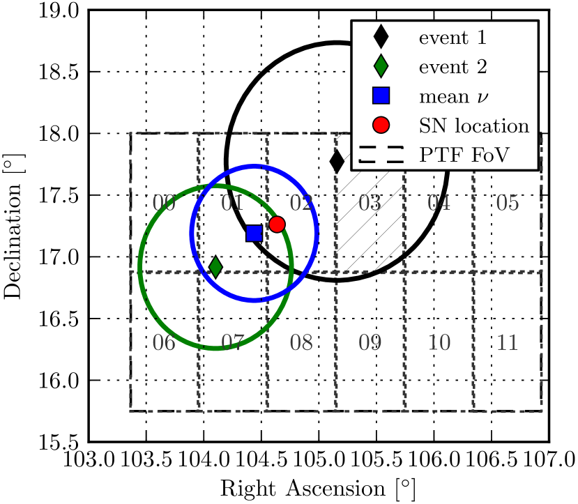
Figure 1.— Map of the sky with the two neutrino event directions, the average neutrino direction, and the location of SN PTF12csy. Estimated reconstruction errors are indicated with circles, the PTF FoV is shown as dashed box. The positions of the PTF survey camera CCD chips are plotted with dotted lines and the chip number is printed on each chip’s field (cf. Law et al. (2009)). Note that chip 03 is not operational and thus hatched in the plot.

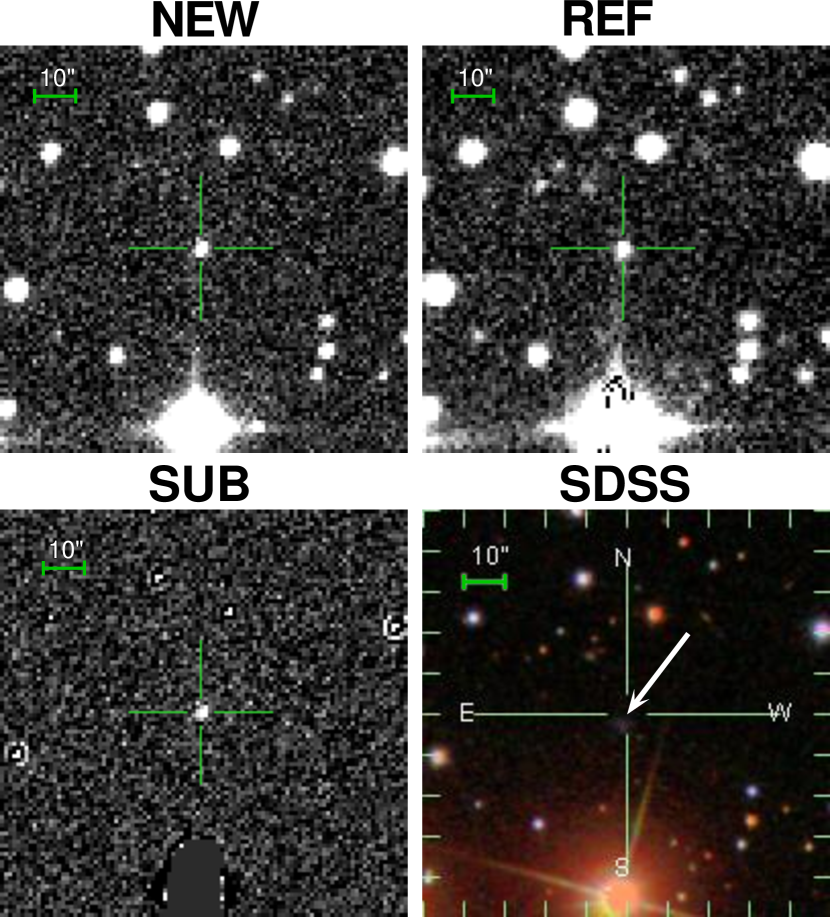
Figure 2.— New image, reference image and post-subtraction image of the PTF discovery of PTF12csy from 2012 April 09, with the location of PTF12csy in the center. This image shows only a small fraction of the PTF FoV. The image from the Sloan Digital Sky Survey (SDSS-III) DR12 (Eisenstein et al., 2011; Gunn et al., 2006; Ahn et al., 2014; Alam et al., 2015) is shown for reference, showing a faint host galaxy to the south of the SN.

However, steady neutrino emission on a time scale of several months is a possibility and explored in Section 4.1.

3.1. Significance of Alert and SN Detection

The value of the test statistic $\lambda$ for the neutrino doublet amounts to $-18.1$. The background distribution of $\lambda$ is constructed from experimental data, containing mostly atmospheric neutrinos, by randomly permuting (shuffling) the event times and calculating equatorial coordinates, i.e. right ascension and declination, from local coordinates, i.e. zenith and azimuth angle, using the new times. That way, all detector effects are entirely preserved, e.g. the distribution of the azimuth angle, which has more events at angles where detector strings are aligned, and the time distribution, which is affected by seasonal variations. At the same time, all potential correlations between the events in time and space, and thus a potential signal, are destroyed.

The false alarm rate (FAR) for an alert with $\lambda\leq-18.1$ is $0.226\text{\,}\mathrm{y}\mathrm{r}^{-1}$, calculated via integration of the $\lambda$ distribution below $-18.1$. Considering the OFU live time of 220.1 days in the data acquisition season of the alert, September 2011 to May 2012, yields $N(\lambda<-18.1)=0.136$ false alerts. Hence, the probability, or p-value, for one or more alerts at least as signal-like to happen by chance in this period is $1-P_{\mathrm{Poisson}}(0;N(\lambda<-18.1))\approx 12.7\%$. The OFU system had already been sending alerts to PTF for $\sim 460$ days at the time of the alert. Scaling up the number of expected alerts with $\lambda\leq-18.1$, one derives a probability of $\sim 24\%$ during 460 days.

The estimated explosion time of SN PTF12csy does not fall within the a priori defined time window for a neutrino-SN coincidence of ${\cal O}($1\text{\,}\mathrm{d}\mathrm{a}\mathrm{y}$)$. It is thus not considered an a priori detection of the follow-up program. Despite this fact, for illustrative purposes, we calculate the a posteriori probability that a random core-collapse SN (CCSN) of any type, at any stage after explosion, is found coincidentally within the error radius of this neutrino doublet and within the luminosity distance of PTF12csy, i.e. $300\text{\,}\mathrm{M}\mathrm{p}\mathrm{c}$. The number of such random SN detections is

$$\overline{N}_{\mathrm{det}}=\frac{\Omega_{s}}{4\pi}\int_{0}^{$300\text{\,}\mathrm{M}\mathrm{p}\mathrm{c}$}\frac{dN_{\mathrm{SN}}}{dt\,dV}\;T(m_{\mathrm{lim}},\hat{M},r)\;4\pi r^{2}\,dr$$ (2)

where $\Omega_{s}$ is the solid angle of the doublet error circle (blue circle in Fig. 1), which is $\sim$0.93\text{\,}\mathrm{(}\mathrm{\SIUnitSymbolDegree}\mathrm{)}^{2}$$. For the volumetric CCSN rate $dN_{\mathrm{SN}}/(dt\,dV)$, a value of $0.78\text{\times}{10}^{-4}\text{\,}\mathrm{M}\mathrm{p}\mathrm{c}^{-3}\,\mathrm{y}\mathrm{r}^{-1}$ is used, Horiuchi et al. (see 2013, sec. 4.1). The control time $T(m_{\mathrm{lim}},\hat{M},r)$ is the average time window in which a SN is detectable, i.e. brighter than the limiting magnitude. It depends on the distance to the source $r$, the peak absolute magnitude $\hat{M}$ of the SN, the limiting magnitude $m_{\mathrm{lim}}$ of the telescope, and the shape of the light curve which is adopted from a SN template web page by P. E. Nugent. It is assumed that $\hat{M}$ follows a Gaussian distribution with mean $-17.5\text{\,}\mathrm{m}\mathrm{a}\mathrm{g}$ and standard deviation $\sigma=$1\text{\,}\mathrm{m}\mathrm{a}\mathrm{g}$$, based on Richardson et al. (2002). For PTF, $m_{\mathrm{lim}}=$19.5\pm 1\text{\,}\mathrm{m}\mathrm{a}\mathrm{g}$$ is assumed.

The resulting expectation value for coincidental SN detections is $\overline{N}_{\mathrm{det}}\approx 0.016$, which results in a Poisson probability of $\sim 1.6\%$ to detect any CCSN within the neutrino alert’s error radius. Combining this probability with the probability of $12.7\%$ for the neutrino alert, Fisher’s method (Brown, 1975; Littell & Folks, 1971; Fisher, 1950, 1990) delivers a combined p-value of $1.4\%$, corresponding to a significance of . For the total live time of 460 days, the combined p-value is $2.5\%$ which corresponds to a significance. This means, even ignoring the a posteriori nature of the p-value, a chance coincidence of the neutrino doublet and the SN detection cannot be ruled out and thus we consider the SN detection to be coincidental.

The following section reports about the available high-energy follow-up data. Limits on a possible long-term neutrino emission from PTF12csy are set using one year of IceCube data. Limits on the X-ray flux were obtained using the Swift satellite. Section 5 deals with the analysis of the low-energy optical and UV data as the SN detection is significant and interesting by itself.

4. HIGH-ENERGY FOLLOW-UP DATA

4.1. Offline Analysis of Neutrino Data

Type IIn supernovae, such as PTF12csy, are a promising class of high-energy transients (see Murase et al. (2011)). The expected duration of neutrino emission from SNe IIn is $110$ months, hence it is extremely unlikely that two neutrinos arrive within less than $2\text{\,}\mathrm{s}$, so late after the SN explosion. However, to test the possibility of a long-term emission, a search for neutrinos from PTF12csy within a search window of roughly one year is conducted.

After the core-collapse of a SN IIn, the supernova ejecta are crashing into massive circumstellar medium (CSM) shells, producing a pair of shocks: a forward and a reverse shock. Cosmic rays (CRs) may be accelerated and multi-TeV neutrinos produced, potentially detectable with IceCube. The collisionless shocks generating the neutrinos are expected to generate X-rays as well at late times (see e.g. Katz et al. (2012); Svirski et al. (2012); Ofek et al. (2013)), but no X-rays were detected for PTF12csy, likely because of the large distance to the SN.

Following Murase et al. (2011) and Murase et al. (2014) (see also Katz et al., 2012), we model high-energy neutrino emission from PTF12csy. As a simplified approach, in order to get an order-of-magnitude estimate of the expected event rate, we perform the following calculation: The CSM density profile is calculated using Murase et al. (2014, eq. 4, eq. A4). The proton spectrum is modeled with a power law index $-2$, as in Murase et al. (2014, eq. A7), with a cut-off energy given by the maximum energy of accelerated protons. The latter is determined by comparing the proton acceleration time scale either with the dynamical time scale (Murase et al., 2014, eq. 28), or, if $pp$ energy losses are relevant, with the cooling time scale (Murase et al., 2014, eq. 30). The lower of the two maximum energies is the one that needs to be considered. The proton spectrum is normalized to the total CR energy $E_{\text{CR}}$ by assuming that a fraction of the kinetic energy of the ejecta $E_{\text{ej}}$ is converted into CRs, that is $E_{\text{CR}}=\epsilon_{\text{CR}}E_{\text{ej}}$ (compare Murase et al., 2014, eq. 3, eq. 25, using CSM shell mass $M_{\text{CSM}}\gg$ SN ejecta mass $M_{\text{ej}}$). Other model parameters are the break-out radius $R_{\text{bo}}$ and shock velocity $v_{\text{shock}}$. The expected neutrino spectrum from $pp$ interaction is derived from the semi-analytical description in Kelner et al. (2006), taking into account the meson production efficiency (Murase et al., 2014, eq. 35, eq. 36). It is distance-scaled and folded with IceCube’s effective area from Aartsen et al. (2014b) to obtain the expected number of events. It is found that inserting commonly assumed values (Murase et al., 2014; Margutti et al., 2014; Murase et al., 2011) of $E_{\text{ej}}=10E_{\text{bol}}=$2.1\text{\times}{10}^{51}\text{\,}\mathrm{e}\mathrm{r}\mathrm{g}$$ (with the bolometric energy found in Section 5.2.5), $\epsilon_{\text{CR}}=0.1$, $M_{\text{ej}}=$10\text{\,}\mathrm{M_{\sun}}$$, $R_{\text{bo}}\approx$6\text{\times}{10}^{15}\text{\,}\mathrm{c}\mathrm{m}$$, and $v_{\text{shock}}\approx$5000\text{\,}\mathrm{k}\mathrm{m}\,\mathrm{s}^{-1}$$, on average only $0.07$ IceCube neutrino detections are expected.

Despite the low expectation for the neutrino fluence, we search for a long-term neutrino signal from PTF12csy in the IceCube data. As a more elaborate approach compared to the simplified approximation described above, we test the neutrino emission models A and B given in Fig. 1 of Murase et al. (2011), which are two representative cases of CR accelerating scenarios: Model A corresponds to a CSM shell with a high density of $1\text{\times}{10}^{11}\text{\,}\mathrm{c}\mathrm{m}^{-3}$ at a small radius of $1e15.5\text{\,}\mathrm{c}\mathrm{m}$, while model B is the opposite with a density of $1e7.5\text{\,}\mathrm{c}\mathrm{m}^{-3}$ at radius $1e16.5\text{\,}\mathrm{c}\mathrm{m}$. For the ejecta, a kinetic energy of $1\text{\times}{10}^{51}\text{\,}\mathrm{e}\mathrm{r}\mathrm{g}$, a velocity of $1\text{\times}{10}^{4}\text{\,}\mathrm{k}\mathrm{m}\,\mathrm{s}^{-1}$, and a mass of several solar masses, lower than the CSM mass, are assumed. Model A is close to a scenario explaining superluminous SNe IIn such as SN 2006gy, while model B is a good description for dimmer, but longer lasting SNe like SN 2008iy. Both models have a neutrino energy spectrum close to $E^{-2}$, with a cut-off energy around $70\text{\,}\mathrm{T}\mathrm{e}\mathrm{V}$ for model A, around $84\text{\,}\mathrm{T}\mathrm{e}\mathrm{V}$ for the forward shock (FS) in model B, and around $275\text{\,}\mathrm{T}\mathrm{e}\mathrm{V}$ for the reverse shock (RS) in model B. In model A, only the reverse shock is of importance for CR acceleration. The suggested emission time scales are $$1\text{\times}{10}^{7}\text{\,}\mathrm{s}$=$115\text{\,}\mathrm{d}$$ for model A and $$1e7.8\text{\,}\mathrm{s}$=$366\text{\,}\mathrm{d}$$ for model B (Murase et al., 2011).

Figure 3 shows the model fluences scaled down to a luminosity distance of $308\text{\,}\mathrm{M}\mathrm{p}\mathrm{c}$. We analyze about one year of IceCube data: the entire IceCube 86 strings data acquisition season 2011/12, from 2011 May 13 to 2012 May 15. The long search window is motivated by the large uncertainty on the explosion date (between 2011 March 21 and 2011 October 13) as well as the long duration of neutrino emission for some scenarios like $\sim 700$ days for model B in Murase et al. (2011). For simplicity, we assume that the entire fluence was emitted during the $1\text{\,}\mathrm{y}\mathrm{r}$ search window. We use the neutrino sample of the IceCube optical follow-up system and perform a statistical point source analysis of neutrino events close to the position of the supernova, based on Braun et al. (2008).

Each neutrino candidate event $i$ is given both a signal and background probability $S_{i}$ and $B_{i}$ which are combined in the likelihood function

$${\cal L}(n_{s})=\prod_{i=1}^{N}\frac{n_{s}}{N}S_{i}+\left(1-\frac{n_{s}}{N}\right)B_{i}.$$ (3)

The variable $n_{s}$ is the number of signal events contained in the sample, which is fitted to maximize the likelihood, and $N$ is the total number of selected neutrino candidate events. The signal probability $S_{i}$ is the product of the spatial Gaussian probability density function (PDF) and the energy PDF $P(E_{i}|\phi)$, i.e. the probability of a signal event having reconstructed energy $E_{i}$ given the neutrino spectrum $\phi$ of the source (derived from Monte Carlo simulation):

$$S_{i}(\sigma_{i},\boldsymbol{x}_{i},\boldsymbol{x}_{s},E_{i})=\frac{1}{2\pi\sigma_{i}^{2}}\exp\left(\frac{-|\boldsymbol{x}_{i}-\boldsymbol{x}_{s}|^{2}}{2\sigma_{i}^{2}}\right)P(E_{i}|\phi).$$ (4)

Here, $\sigma_{i}$ is the event’s angular error estimate, $\boldsymbol{x}_{i}$ is the event’s reconstructed direction, and $\boldsymbol{x}_{s}$ the SN or neutrino source position. The background probability $B_{i}$ contains the energy PDF and a normalization constant for the background from atmospheric neutrinos.

We define the test statistic as likelihood ratio (Braun et al., 2008)

$$\lambda=-2\log\left[\frac{{\cal L}(0)}{{\cal L}(\hat{n}_{s})}\right],$$ (5)

serving as a powerful test for separating the null hypothesis from the hypothesis of signal event contribution. Here, $\hat{n}_{s}$ is the number of signal events that maximizes the likelihood and corresponds to the most likely description of the data.

The result of the maximum likelihood fit is $\hat{n}_{s}=0$ both for model A and B, i.e. we see no sign of signal contribution in our neutrino event sample. We set 90% C.L. Neyman upper limits (see Neyman (1937), reprinted in Neyman (1967)) on the tested neutrino fluence models, which amount to $\sim 1500$ and $\sim 1300$ times the fluences given for model A and B above, respectively. The limits are much higher than the fluence prediction because of IceCube being insensitive to SNe IIn at such large distances. Figure 3 shows a plot of the tested neutrino fluence and the limits set using $1\text{\,}\mathrm{y}\mathrm{r}$ of IceCube data.

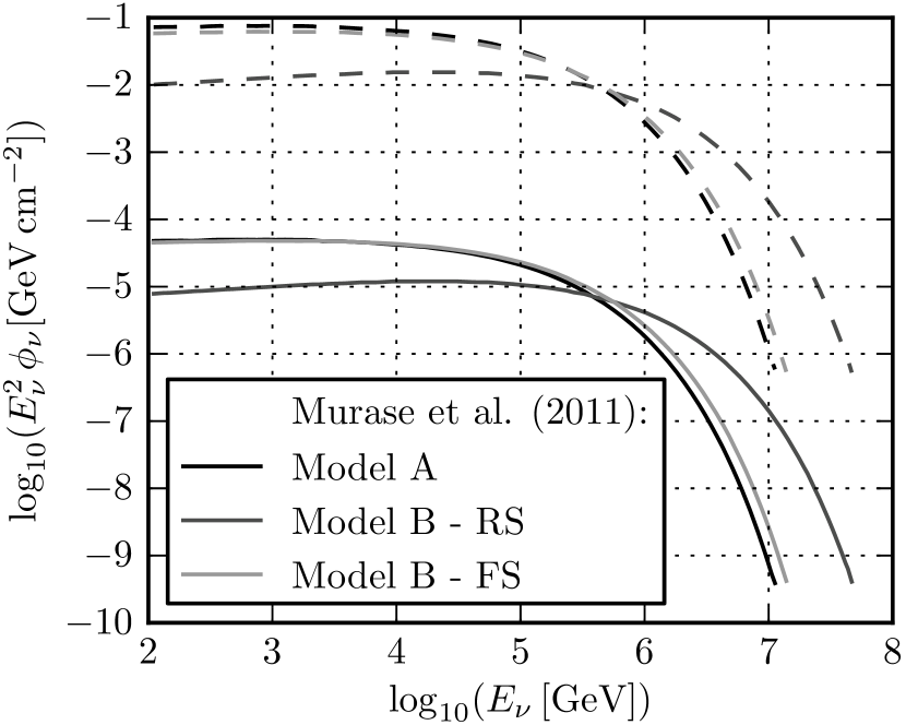
Figure 3.— Neutrino fluence at Earth from PTF12csy (solid lines) and derived upper limits set by IceCube (dashed lines, corresponding gray scales) as function of energy for the tested models A, B reverse shock (RS), and B forward shock (FS) from Murase et al. (2011).

This null result and the large distance to the SN further support our conclusion that the SN detection was coincidental.

Nevertheless, it is interesting to roughly estimate the hypothetical emitted neutrino fluence: We take the median neutrino energies of the two alert neutrinos from Table 1 and look up the effective areas for the OFU neutrino sample at the respective energies. From this, we derive a hypothetical neutrino fluence of $3.2\text{\times}{10}^{-4}\text{\,}\mathrm{e}\mathrm{r}\mathrm{g}\,\mathrm{c}\mathrm{m}^{-2}$ for a source spectrum $\propto E^{-2}$ ($E_{\nu}=$5.4\text{\,}\mathrm{T}\mathrm{e}\mathrm{V}$,$15.7\text{\,}\mathrm{T}\mathrm{e}\mathrm{V}$$), or $10.8\text{\times}{10}^{-4}\text{\,}\mathrm{e}\mathrm{r}\mathrm{g}\,\mathrm{c}\mathrm{m}^{-2}$ for a source spectrum $\propto E^{-3}$ ($E_{\nu}=$0.7\text{\,}\mathrm{T}\mathrm{e}\mathrm{V}$,$1.5\text{\,}\mathrm{T}\mathrm{e}\mathrm{V}$$). Assuming that this neutrino fluence was emitted by the SN, this would imply a radiated neutrino energy of $\sim$3.4\text{\times}{10}^{51}\text{\,}\mathrm{e}\mathrm{r}\mathrm{g}$$ or $\sim$1.2\text{\times}{10}^{52}\text{\,}\mathrm{e}\mathrm{r}\mathrm{g}$$ using the luminosity distance of $\sim$300\text{\,}\mathrm{M}\mathrm{p}\mathrm{c}$$, corresponding to about 15 or about 50 times the radiated electromagnetic energy of $E_{\mathrm{bol}}=$2.1\text{\times}{10}^{50}\text{\,}\mathrm{e}\mathrm{r}\mathrm{g}$$ (see Section 5.2.5). This is higher than what can be expected, since with reasonable assumptions that the explosion energy $E_{\mathrm{ej}}\leq 10E_{\mathrm{bol}}$ (Murase et al., 2014; Margutti et al., 2014) and a fraction $\epsilon_{\mathrm{CR}}\leq 0.1$ of it going into CRs (Murase et al., 2011), the energy in neutrinos should be on the same order or less than $E_{\mathrm{bol}}$. Thus, also with a simple energetic argument, isotropic neutrino emission from PTF12csy causing the neutrino alert is implausible, especially on a time scale of seconds. However, a beamed emission from a jet with a small opening angle of $<$30\text{\,}\mathrm{\SIUnitSymbolDegree}$$ would in principle be possible.

4.2. X-ray Observations of PTF12csy

The Swift satellite observed the supernova four times, on 2012 April 20 (MJD 56037) and around 2012 November 15 (MJD 56246) (see Table 2). We perform source detection using the software developed for the 1SXPS catalog (Evans et al., 2014) on each of the four observations, and on a summed image made by combining all the datasets. No counterpart to PTF12csy is detected. Upper limits are generated for each of these images, following Evans et al. (2014). A $28\text{\,}\arcsec$ radius circle centered on the optical position of PTF12csy is used to measure the detected X-ray counts $c$ at this location, and the expected number of background counts $c_{\text{bg}}$, predicted by the background map created in the source detection process. We then use the Bayesian method of Kraft et al. (1991) to calculate the upper limit $c_{\text{UL}}$ on the X-ray count rate of PTF12csy, using the XRT exposure map to correct for any flux losses due to bad pixels on the XRT detector, and the finite size of the circular region.

The upper limit count rate is converted to unabsorbed flux $\Phi_{\text{UL}}$ using the HEASARC Tool WebPIMMS, assuming a black body model with $T=$0.6\text{\,}\mathrm{k}\mathrm{e}\mathrm{V}$$ as in Miller et al. (2010b), a Galactic hydrogen column density of $1.31\text{\times}{10}^{21}\text{\,}\mathrm{c}\mathrm{m}^{-2}$ (Willingale et al., 2013) and a redshift of $z=0.0684$. The result is a $0.210\text{\,}\mathrm{k}\mathrm{e}\mathrm{V}$ X-ray flux $<$4.6\text{\times}{10}^{-14}\text{\,}\mathrm{e}\mathrm{r}\mathrm{g}\,\mathrm{c}\mathrm{m}^{-2}\,\mathrm{s}^{-1}$$ for the most constraining upper limits, corresponding to a $0.210\text{\,}\mathrm{k}\mathrm{e}\mathrm{V}$ X-ray luminosity of $L_{X}<$5.2\text{\times}{10}^{41}\text{\,}\mathrm{e}\mathrm{r}\mathrm{g}\,\mathrm{s}^{-1}$$ with a luminosity distance of about $308\text{\,}\mathrm{M}\mathrm{p}\mathrm{c}$. Using a power-law $\propto E^{-2}$ instead of a black body as an alternative X-ray emission model, the unabsorbed flux upper limit becomes $<$7.4\text{\times}{10}^{-14}\text{\,}\mathrm{e}\mathrm{r}\mathrm{g}\,\mathrm{c}\mathrm{m}^{-2}\,\mathrm{s}^{-1}$$, and hence, $L_{X}<$8.4\text{\times}{10}^{41}\text{\,}\mathrm{e}\mathrm{r}\mathrm{g}\,\mathrm{s}^{-1}$$.

Table 2Swift XRT observations of PTF12csy

Time ($\mathrm{M}\mathrm{J}\mathrm{D}$)	Exposure ($\mathrm{ks}$)	$c$	$c_{\text{bg}}$	$c_{\text{UL}}$	$\Phi_{\text{UL}}$
56037.15	4.9	1	1.47	1.3	$4.6$
56245.29	2.0	1	0.62	2.1	$7.4$
56246.04	1.2	2	0.44	9.8	$30.0$
56247.62	5.0	2	1.35	2.1	$7.4$
Sum	13.0	6	3.71	1.3	$4.6$

Note. — Energy range: $0.210\text{\,}\mathrm{k}\mathrm{e}\mathrm{V}$. $c$: measured counts within a $28\text{\,}\arcsec$ aperture. $c_{\text{bg}}$: expected background counts within the same aperture. $c_{\text{UL}}$: upper limit on the X-ray count rate in $\mathrm{1}\mathrm{0}^{-3}\,\mathrm{s}^{-1}$. $\Phi_{\text{UL}}$: upper limit on the unabsorbed source flux in $\mathrm{1}\mathrm{0}^{-14}\,\mathrm{e}\mathrm{r}\mathrm{g}\,\mathrm{c}\mathrm{m}^{-2}\,\mathrm{s}^{-1}$.

Comparing with other SNe IIn, e.g. SN 2008iy (Miller et al., 2010b) which had a measured X-ray luminosity of $L_{X}=$(2.4\pm 0.8)\text{\times}{10}^{41}\text{\,}\mathrm{e}\mathrm{r}\mathrm{g}\,\mathrm{s}^{-1}$$ or SN 2010jl (Ofek et al., 2014b) with $L_{X}\approx$1.5\text{\times}{10}^{41}\text{\,}\mathrm{e}\mathrm{r}\mathrm{g}\,\mathrm{s}^{-1}$$, we cannot exclude X-ray emission from PTF12csy with our measured upper limit. However, Svirski et al. (2012) suggest that $L_{X}$ be about $10^{-4}$ of the bolometric luminosity at the time of the shock breakout. With the estimated bolometric luminosity from Section 5.2.5 around the time of the first Swift observations, this implies $L_{X}\approx$6.4\text{\times}{10}^{38}\text{\,}\mathrm{e}\mathrm{r}\mathrm{g}\,\mathrm{s}^{-1}$$, well below our X-ray limits.

5. LOW-ENERGY FOLLOW-UP DATA

5.1. Optical and UV Observations of PTF12csy

During the follow-up program of the neutrino alert, the first observations were done on 2012 April 03, 05, 07 and 09 (MJD 56020 to 56026) by PTF with the Palomar Samuel Oschin 48-inch telescope (P48) (Law et al., 2009), which is a wide-field Schmidt telescope. The images (see Fig. 2) revealed a so far undiscovered supernova, named PTF12csy, at a magnitude of $\sim 18.6$ in the Mould $R$-band. More photometric observations were carried out, with the P48 and the Palomar 60-inch (P60) telescopes (Law et al., 2009) at the Palomar Observatory in California, and the Faulkes Telescope North (FTN) (Brown et al., 2013) at Haleakala on Maui, Hawaii. Spectroscopy was taken as well, with the Gemini North Multi-Object Spectrograph (GMOS) (Hook et al., 2004) on the $8\text{\,}\mathrm{m}$ Gemini North telescope (Mauna Kea, Hawaii) on 2012 April 17 (MJD 56034) and with the Low-Resolution Imaging Spectrometer (LRIS) (Oke et al., 1995) on the $10\text{\,}\mathrm{m}$ Keck I telescope (Kamuela, Hawaii) on 2013 February 09 (MJD 56332), enabling the identification of the supernova as a Type IIn SN with narrow emission lines. The spectra are available from WISeREP (Yaron & Gal-Yam, 2012).

P48 data were extracted using an aperture photometry pipeline and are calibrated with 21 close-by SDSS stars (Eisenstein et al., 2011; Gunn et al., 2006; Ahn et al., 2014; Alam et al., 2015). The faint host galaxy was subtracted and the upper limits are at the level. P48 magnitudes are in the PTF natural AB magnitude system, which is similar, but not identical to the SDSS system. The difference is given by a color term, which is ignored in this work, except for the conversion of Mould $R$ to SDSS $r$, explained in Section 5.2.1. The P60 photometry is tied to the same 21 SDSS calibration stars. Note that there might be host galaxy contamination in the late-epoch P60 photometry. P60 magnitudes are in the SDSS AB magnitude system. The FTN data were processed by an automatic pipeline, without host subtraction, and agree very well with the host-subtracted P60 data taken in the same night.

The Pan-STARRS1 (PS1) telescope was not part of the real-time triggering and response system, but its wide-field coverage provides a useful archive to search retrospectively for detections. PS1 is a $1.8\text{\,}\mathrm{m}$ telescope located at Haleakala on Maui in the Hawaiian islands, equipped with a $3.3\text{\,}\mathrm{\SIUnitSymbolDegree}$ FOV and a 1.4 gigapixel camera (Kaiser, 2004). In the course of its 3$\pi$ steradian survey, the telescope observes each part of the sky typically $810$ times per year (Magnier et al., 2013). PS1 first detected PTF12csy on MJD $55\,847.582$ and archived it as object PSO J104.6365+17.2622. The magnitudes in all PS1 images were obtained with PSF fitting within the Pan-STARRS Image Processing Pipeline (Magnier, 2006). They are calibrated to typically seven local SDSS DR8 field stars. The magnitudes are in the natural PS1 AB system as defined in Tonry et al. (2012), which is similar, but not exactly the same as SDSS AB magnitudes. Particularly the $g$-band can differ.

The Swift UVOT data were analyzed using the publicly available Swift analysis tools (Nasa High Energy Astrophysics Science Archive Research Center (2014), Heasarc), and a source was seen close to the detection threshold.

ROTSE’s limiting magnitude of about $1617\text{\,}\mathrm{m}\mathrm{a}\mathrm{g}$ prevented a detection of the SN in ROTSE follow-up observations.

5.2. Photometry

5.2.1 Photometric Corrections

The photometry is corrected for Galactic extinction using $R_{V}=A_{V}/E(B-V)=3.1$ and $E(B-V)=0.071$ (Schlegel et al., 1998). The extinction coefficient is converted to the filters’ effective wavelengths using the algorithm from Cardelli et al. (1989), i.e. $0.35\text{\,}\mathrm{m}\mathrm{a}\mathrm{g}$ for $u$, $0.30\text{\,}\mathrm{m}\mathrm{a}\mathrm{g}$ for $B$, $0.26\text{\,}\mathrm{m}\mathrm{a}\mathrm{g}$ for $g$, $0.19\text{\,}\mathrm{m}\mathrm{a}\mathrm{g}$ for $r$, $0.11\text{\,}\mathrm{m}\mathrm{a}\mathrm{g}$ for $z$. The extinction within the host galaxy could not be determined.

In Fig. 4, the Gemini North spectrum is overlaid with the applied photometric filters. The strong Balmer lines contribute differently to the various filters. For the SED construction (see Section 5.2.5), in order to approximate the black body continuum, the contribution of the strongest emission lines, H$\alpha$ and H$\beta$, is removed from the photometry using the Gemini North spectrum and the filter curves. For Figs. 6 and 7, the P48 Mould $R$ magnitudes are converted to SDSS $r$ by subtracting the H$\alpha$ contribution (as above), applying the formulae in Ofek et al. (2012) valid for black body spectra, and then re-adding the H$\alpha$ contribution to the $r$-band. After conversion, the P48 $R$ magnitudes are consistent with the P60 SDSS $r$ magnitudes.

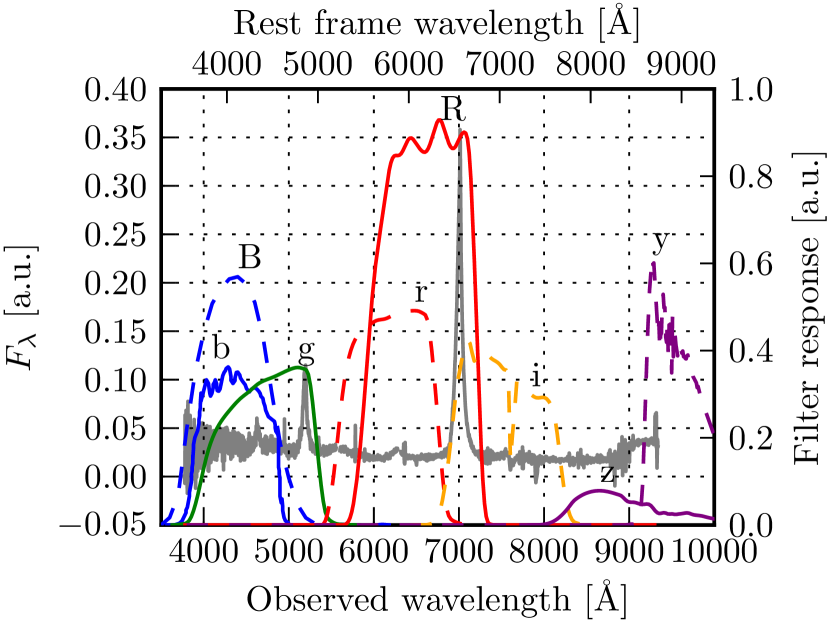
Figure 4.— Background, gray, left axis: Gemini North spectrum from 2012 April 17 (MJD 56034). Foreground, multiple colors, right axis: The filter response functions of the applied photometric filters, defined as filter transmission or effective area. Note that the absolute normalization is arbitrary and only the shape of the curves is relevant.

The Swift UVOT data contain host contamination. Since no GALEX data from a pre- or post-SN epoch are available for the host galaxy, no host subtraction can be done in the UV filters of UVOT. For the $u$, $b$ and $v$ filters, the host is subtracted by interpolating the host magnitudes from the SDSS DR12 data (Alam et al., 2015) to the effective wavelengths of the UVOT filters.

5.2.2 The Light Curves

The earliest detection of PTF12csy was in the Pan-STARRS1 y-band on 2011 October 13 (MJD $55\,847.582$), 169 days prior to the neutrino alert in observer frame, corresponding to 158 days in host galaxy rest frame using $z=0.0684$ (see Section 5.3). The latest non-detection, again in Pan-STARRS1, was on 2011 March 21 (MJD 55641.3) in a $30\text{\,}\mathrm{s}$ $z$-band frame, 206 days before the first detection (193 days in rest frame). Hence, the explosion time is not well constrained and can be anytime between MJD 55641.3 and MJD $55\,847.6$. Hereafter, we refer to the $y$-band detection at MJD $55\,847.582$ as the first detection and use it as day 0 for the light curve.

The uncorrected SN light curves with the data available through the IceCube optical follow-up program are displayed in Fig. 5, including photometry acquired with the Swift UVOT filters $uvw2$, $uvm2$, $uvw1$, $u$ and $b$; the Johnson $B$ filter on P60; the SDSS filters $g$, $r$, $i$ with data from P60, PS1, and FTN; the SDSS $z$ filter on P60; Mould $R$ filter on P48; and Pan-STARRS $y$ filter on PS1. The entire uncorrected photometry in apparent magnitudes, as seen in Fig. 5, is also available in Table 3. The light curves are averaged within bins of 10 days width, for each filter and telescope separately. Note that, in contrast to most of the other photometry, no host subtraction is performed for the Swift UVOT magnitudes presented in Fig. 5 and Table 3.

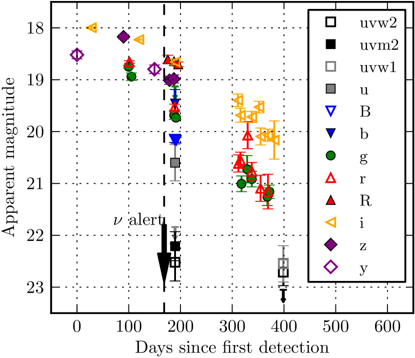
Figure 5.— PTF12csy photometry in apparent magnitudes without applying corrections. The photometry is averaged over intervals of 10 days. The data originate from the following telescopes: $uvw2$, $uvm2$, $uvw1$, $u$, $b$: UVOT; $B$: P60; $g$: P60, PS1, FTN; $r$: P60, PS1, FTN; $R$: P48; $i$: P60, PS1, FTN; $z$: P60, PS1; $y$: PS1.

Table 3Photometric observations of PTF12csy

MJD Date	Rest frame days	Mag	Abs. mag	Lim. mag	Filter	Tel.
$55\,273.219$	$-537.589$	$\cdots$	$\cdots$	$21.11$	$g$	P48
$55\,294.162$	$-517.987$	$\cdots$	$\cdots$	$20.62$	$R$	P48
$55\,431.514$	$-389.429$	$\cdots$	$\cdots$	$18.99$	$R$	P48
$55\,477.402$	$-346.478$	$\cdots$	$\cdots$	$20.67$	$R$	P48
$55\,596.889$	$-234.642$	$\cdots$	$\cdots$	$18.90$	$g$	P48
$55\,641.304$	$-193.071$	$\cdots$	$\cdots$	$21.40$	$z$	PS1
$55\,847.588$	$0.005$	$18.52\pm 0.08$	$-18.92$	$\cdots$	$y$	PS1
$55\,875.515$	$26.145$	$18.00\pm 0.02$	$-19.45$	$\cdots$	$i$	PS1
$55\,937.502$	$84.163$	$18.17\pm 0.04$	$-19.27$	$\cdots$	$z$	PS1
$55\,948.816$	$94.752$	$18.82\pm 0.05$	$-18.62$	$\cdots$	$g$	PS1
$55\,948.841$	$94.776$	$18.66\pm 0.02$	$-18.79$	$\cdots$	$r$	PS1
$55\,957.475$	$102.858$	$19.00\pm 0.02$	$-18.44$	$\cdots$	$g$	PS1
$55\,967.269$	$112.024$	$18.23\pm 0.01$	$-19.22$	$\cdots$	$i$	PS1
$55\,997.366$	$140.194$	$18.80\pm 0.08$	$-18.64$	$\cdots$	$y$	PS1
$56\,022.981$	$164.169$	$18.61\pm 0.08$	$-18.84$	$18.23$	$R$	P48
$56\,026.246$	$167.225$	$19.01\pm 0.08$	$-18.43$	$\cdots$	$z$	PS1
$56\,034.841$	$175.270$	$19.47\pm 0.04$	$-17.98$	$\cdots$	$r$	P60
$56\,034.844$	$175.273$	$18.99\pm 0.08$	$-18.46$	$\cdots$	$z$	P60
$56\,035.177$	$175.584$	$18.64\pm 0.04$	$-18.80$	$\cdots$	$R$	P48
$56\,035.922$	$176.281$	$18.68\pm 0.03$	$-18.76$	$\cdots$	$i$	P60
$56\,035.925$	$176.284$	$20.15\pm 0.06$	$-17.30$	$\cdots$	$B$	P60
$56\,035.928$	$176.287$	$19.69\pm 0.05$	$-17.75$	$\cdots$	$g$	P60
$56\,036.581$	$176.899$	$18.66\pm 0.04$	$-18.78$	$20.97$	$i$	FTN
$56\,036.585$	$176.902$	$19.54\pm 0.06$	$-17.90$	$21.12$	$r$	FTN
$56\,036.590$	$176.906$	$19.73\pm 0.07$	$-17.72$	$21.23$	$g$	FTN
$56\,037.150$	$177.431$	$\cdots$	$\cdots$	$19.13$	$v$	UVOT
$56\,037.150$	$177.431$	$20.60\pm 0.35$	$-16.84$	$20.79$	$u$	UVOT
$56\,037.150$	$177.431$	$22.21\pm 0.28$	$-15.23$	$22.76$	$uvm2$	UVOT
$56\,037.150$	$177.431$	$22.52\pm 0.36$	$-14.92$	$22.71$	$uvw2$	UVOT
$56\,037.150$	$177.431$	$\cdots$	$\cdots$	$21.84$	$uvw1$	UVOT
$56\,037.150$	$177.431$	$19.46\pm 0.27$	$-17.98$	$19.95$	$b$	UVOT
$56\,039.175$	$179.326$	$18.74\pm 0.03$	$-18.70$	$\cdots$	$i$	P60
$56\,039.177$	$179.328$	$19.55\pm 0.04$	$-17.89$	$\cdots$	$r$	P60
$56\,039.178$	$179.329$	$20.17\pm 0.06$	$-17.28$	$\cdots$	$B$	P60
$56\,039.181$	$179.332$	$19.73\pm 0.04$	$-17.71$	$\cdots$	$g$	P60
$56\,040.285$	$180.365$	$18.60\pm 0.07$	$-18.85$	$20.98$	$i$	FTN
$56\,043.178$	$183.073$	$18.70\pm 0.05$	$-18.74$	$\cdots$	$R$	P48
$56\,158.504$	$291.015$	$19.40\pm 0.12$	$-18.05$	$\cdots$	$i$	P60
$56\,161.496$	$293.815$	$20.58\pm 0.12$	$-16.86$	$\cdots$	$r$	P60
$56\,163.490$	$295.682$	$19.69\pm 0.13$	$-17.76$	$\cdots$	$i$	P60
$56\,165.486$	$297.550$	$21.01\pm 0.15$	$-16.44$	$\cdots$	$g$	P60
$56\,176.465$	$307.826$	$20.73\pm 0.26$	$-16.72$	$\cdots$	$g$	P60
$56\,177.453$	$308.751$	$20.07\pm 0.26$	$-17.37$	$\cdots$	$r$	P60
$56\,185.431$	$316.218$	$19.72\pm 0.11$	$-17.73$	$\cdots$	$i$	P60
$56\,185.432$	$316.219$	$20.77\pm 0.17$	$-16.68$	$\cdots$	$r$	P60
$56\,185.436$	$316.223$	$20.92\pm 0.15$	$-16.53$	$\cdots$	$g$	P60
$56\,200.887$	$330.685$	$19.81\pm 0.30$	$-17.63$	$\cdots$	$i$	P60
$56\,202.385$	$332.086$	$21.09\pm 0.25$	$-16.35$	$\cdots$	$r$	P60
$56\,215.381$	$344.250$	$21.23\pm 0.39$	$-16.21$	$\cdots$	$r$	P60
$56\,215.429$	$344.295$	$20.11\pm 0.10$	$-17.33$	$\cdots$	$i$	P60
$56\,215.435$	$344.301$	$21.25\pm 0.17$	$-16.19$	$\cdots$	$g$	P60
$56\,219.344$	$347.960$	$21.16\pm 0.13$	$-16.28$	$\cdots$	$g$	P60
$56\,219.837$	$348.421$	$20.97\pm 0.13$	$-16.47$	$\cdots$	$r$	P60
$56\,224.988$	$353.242$	$20.01\pm 0.17$	$-17.44$	$\cdots$	$i$	P60
$56\,229.808$	$357.754$	$20.20\pm 0.45$	$-17.24$	$\cdots$	$i$	P60
$56\,246.320$	$373.208$	$22.71\pm 0.26$	$-14.73$	$23.34$	$uvw2$	UVOT
$56\,246.320$	$373.208$	$22.55\pm 0.35$	$-14.89$	$22.79$	$uvw1$	UVOT
$56\,246.320$	$373.208$	$\cdots$	$\cdots$	$23.05$	$uvm2$	UVOT

Note. — Rest frame days relative to first detection on MJD $55\,847.582$. 10-day binning. No correction for extinction.

Figure 6 shows the light curve of selected filters in absolute magnitudes, after the photometric corrections. Light curves of other exceptional Type II SNe are overlaid for comparison: SN IIn 2006gy (Ofek et al., 2007; Smith et al., 2007; Kawabata et al., 2009; Miller et al., 2010a), one of the most luminous SNe ever recorded, and SN 2010jl (Stoll et al., 2011; Zhang et al., 2012), a SN IIn that is spectroscopically similar to PTF12csy (see Section 5.3) and shows signs of a collisionless shock in an optically thick circumstellar medium (CSM), hinting towards potential high-energy neutrino production (Ofek et al., 2013). Note that the SN 2010jl light curve is not extinction corrected and the comparison light curves have different reference dates: SN 2010jl is relative to maximum light, 2006gy is relative to the explosion time. A theoretical light curve from pure radioactive decay of ${}^{56}\text{Ni}\rightarrow{}^{56}\text{Co}\rightarrow{}^{56}\text{Fe}$ (black dashed line) is added to the figure as well, scaled to match the observed absolute magnitude of PTF12csy.

The brightest observed absolute magnitudes after application of photometric corrections (see Section 5.2.1) and converting to absolute magnitudes with a distance modulus of $\mu=37.443$ ($z=0.0684$) are $M_{g}\approx$-19.0\text{\,}\mathrm{m}\mathrm{a}\mathrm{g}$$, $M_{r}\approx$-19.0\text{\,}\mathrm{m}\mathrm{a}\mathrm{g}$$, $M_{i}\approx$-19.6\text{\,}\mathrm{m}\mathrm{a}\mathrm{g}$$, $M_{z}\approx$-19.4\text{\,}\mathrm{m}\mathrm{a}\mathrm{g}$$, and $M_{y}\approx$-19.0\text{\,}\mathrm{m}\mathrm{a}\mathrm{g}$$, assuming standard cosmology with Hubble parameter $H_{0}=$70\text{\,}\mathrm{k}\mathrm{m}\,\mathrm{s}^{-1}\,\mathrm{M}\mathrm{p}\mathrm{c}^{-1}$$, matter density $\Omega_{m}=0.3$, and dark energy density $\Omega_{\Lambda}=0.7$. While these are lower limits to the peak magnitude due to the sparse sampling, these absolute magnitudes are relatively modest compared to the most luminous SNe IIn, e.g. SN 2006gy ($M_{R}=$-22\text{\,}\mathrm{m}\mathrm{a}\mathrm{g}$$) (Kawabata et al., 2009) or SN 2008fz ($M_{V}=$-22.3\text{\,}\mathrm{m}\mathrm{a}\mathrm{g}$$) (Drake et al., 2010). They are however comparable to the SNe IIn 2008iy ($M_{r}\approx$-19.1\text{\,}\mathrm{m}\mathrm{a}\mathrm{g}$$) (Miller et al., 2010b), 1988Z ($M_{R}\lesssim$-18.9\text{\,}\mathrm{m}\mathrm{a}\mathrm{g}$$) (Turatto et al., 1993) and SN 2010jl ($M_{R}\lesssim$-20.0\text{\,}\mathrm{m}\mathrm{a}\mathrm{g}$$) (Zhang et al., 2012).

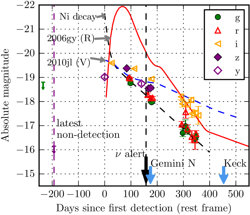
Figure 6.— PTF12csy photometry (symbols) in absolute magnitudes, with correction for Galactic extinction, and conversion of P48 Mould R magnitudes to SDSS $r$ magnitudes (see Section 5.2.1). The data originate from the following telescopes: $g$: P48, P60, PS1, FTN; $r$: P48, P60, PS1, FTN; $i$: P60, PS1, FTN; $z$: P60, PS1; $y$: PS1. The photometry is averaged over intervals of 10 days. Other absolute SN II light curves (lines) and a theoretical light curve from radioactive decay of nickel (black dashed line) are added for comparison. The comparison light curves are partly not extinction corrected and have different reference dates (see text).

5.2.3 Decline Rates and Energy Source

The light curves of PTF12csy indicate a plateau within $\sim$100\text{\,}\mathrm{d}\mathrm{a}\mathrm{y}\mathrm{s}$$ after first detection, and a slow fading afterwards. The corrected absolute magnitude light curves are fitted to obtain the linear decline rates in different photometric filters, during different epochs (see Fig. 7 and Table 4). For some epochs and filters, especially $g$ and $r$, the decline rates are close to $0.98\text{\,}\mathrm{m}\mathrm{a}\mathrm{g}\,\mathrm{(}\mathrm{1}\mathrm{0}\mathrm{0}\mathrm{d}\mathrm{a}\mathrm{y}\mathrm{s}\mathrm{)}^{-1}$, the decline rate expected for radioactive ⁵⁶Co decay (Miller et al., 2010b), while in general decline rates are slower, indicating that at least part of the radiated energy is powered by interaction of the SN ejecta with a dense CSM (Miller et al., 2010b).

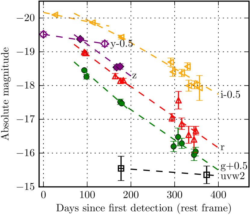
Figure 7.— Light curves of several filters with the fitted linear declines. See Table 4 for the numerical values of the found decline rates.

Table 4Decline rates of the PTF12csy light curve

Filter	$0150\text{\,}\mathrm{d}$	$70200\text{\,}\mathrm{d}$	$170400\text{\,}\mathrm{d}$
$uvw2$	$\cdots$	$\cdots$	$0.097\pm 0.227$
$g$	$\cdots$	$1.127\pm 0.044$	$0.893\pm 0.051$
$r$	$\cdots$	$0.974\pm 0.053$	$0.907\pm 0.059$
$i$	$0.269\pm 0.024$	$0.656\pm 0.089$	$0.764\pm 0.052$
$z$	$\cdots$	$0.943\pm 0.079$	$\cdots$
$y$	$0.199\pm 0.080$	$\cdots$	$\cdots$

Additionally, radioactive decay of ⁵⁶Co at a still relatively high absolute magnitude of $\sim$-19\text{\,}\mathrm{m}\mathrm{a}\mathrm{g}$$ implies a preceding ⁵⁶Ni decay with an extremely bright peak, which was not observed, although the data are quite sparse. Assuming that the luminosity is generated by radioactive decay alone and following Kulkarni (2005), we estimate that $\gtrsim$1.7\text{\,}\mathrm{M_{\sun}}$$ of ⁵⁶Ni would be required to provide the bolometric luminosity of $9.7\text{\times}{10}^{42}\text{\,}\mathrm{e}\mathrm{r}\mathrm{g}\,\mathrm{s}^{-1}$ at $100\text{\,}\mathrm{d}$ in rest frame (see Section 5.2.5). The lower limit on the ⁵⁶Ni mass is set by assuming that the explosion and thus generation of ⁵⁶Ni was at the latest possible time, directly before the first detection. Figure 6 shows the corresponding theoretical light curve resulting from the radioactive decay of nickel and cobalt (black dashed line). Adopting an earlier explosion time results in an even larger ⁵⁶Ni mass.

This is much more than the usual amount of ⁵⁶Ni of $<0.5\text{\,}\mathrm{M_{\sun}}$, often $<0.1\text{\,}\mathrm{M_{\sun}}$ (see e.g. Pejcha & Thompson (2015), also Margutti et al. (2014)). However, extremely superluminous SNe might have ⁵⁶Ni masses of that order of magnitude (Gal-Yam, 2012).

We note that in addition to the ⁵⁶Ni mass and luminosity arguments, the spectrum showing intermediate width Balmer lines and a continuum appears inconsistent with radioactive decay as well (see Section 5.3).

5.2.4 Fitting to an Interaction Model

Here we assume that the light curve is powered by conversion of the ejecta’s kinetic energy to luminosity through interaction of the ejecta with the CSM. Following Ofek et al. (2014b, see also: e.g. ()), we model the light curve as a power-law of the form $L(t)=L_{0}t^{\alpha}$.

After shock breakout, there is a phase of power-law decline of the luminosity, with an index of typically $\alpha\approx-0.3$. This lasts until the shock runs over a CSM mass equivalent to the ejecta mass and the shock enters a new phase of either conservation of energy if the density is low enough and the gas cannot cool quickly (the Sedov-Taylor phase), or conservation of momentum if the gas radiates its energy via fast cooling (the snow-plow phase). During the late stage, the light curve will be declining more steeply, in both cases (Ofek et al., 2014b).

Since we assume PTF12csy to be powered by interaction, we try to fit the interaction model from Ofek et al. (2014b) to the light curve data with the least-squares method. We perform the fit within the range of $93200$ rest frame days, starting at the first r-band detection, and use the r-band light curve scaled with the bolometric luminosity from Section 5.2.5. It is found that the power-law index $\alpha$ needs to be significantly steeper than $-0.3$ in order to reasonably describe the data. It lies in the range of $-3-1.2$, using the constraint on the explosion time (see Section 5.2.2) for the temporal zero point of the power-law. The best fit is at $\alpha=-3$, with the explosion time at the lowest allowed value which is the date of the last non-detection. This suggests a very steep CSM density profile $\propto r^{-5}$ (see Ofek et al., 2014b, eq. 12), compared to the profile $\propto r^{-2}$ resulting from a wind with steady mass loss. However, the self-similar solutions of the hydrodynamical equations (Chevalier, 1982) that are used in Ofek et al. (2014b, eq. 12) are invalid if the CSM density profile is steeper than $r^{-3}$. But nevertheless, as discussed for the late-time light curve in Ofek et al. (2014b, sec. 5.2), probably the profile is steeper than $r^{-3}$.

This leaves us with several possible explanations:

1. Already between rest frame days 93 and 200, the SN was in the late, e.g. snow-plow, phase. This is consistent with SN 2010jl, where the late-time light curve also shows a power-law index $\alpha\approx-3$ (Ofek et al., 2014b, sec. 5.2). Assuming that the break in the light curve between power-law phase and late phase occurred just before the first r-band detection at day 93, and comparing with SN 2010jl (Ofek et al., 2014b), then this means that the SN was likely already a few hundred days old, and the r-band maximum was about $11.25$ $\mathrm{m}\mathrm{a}\mathrm{g}$ brighter than the observed one (cf. Ofek et al., 2014b, Fig. 1), consistent with SN 2010jl’s r-band maximum. It follows that the power-law phase ended $\leq 286$ rest frame days after explosion, from which we can derive a swept CSM mass of $\lesssim$12\text{\,}\mathrm{M_{\sun}}$$, using Ofek et al. (2014b, eq. 22) and adopting the standard values given for SN 2010jl.

2. The SN is powered by ejecta-CSM interaction, but its light curve is declining steeper than a $t^{-0.3}$ power-law. This is possible, e.g. if spherical symmetry, assumed in Ofek et al. (2014b), is broken, if the optical depth is lower than in SN 2010jl or if the CSM density profile falls steeper than $r^{-2}$ (s.a.).

3. The SN is not powered by interaction, but by radioactive decay, leading to an exponential light curve decline. However, this appears unlikely, as noted above in Section 5.2.3.

5.2.5 Spectral Energy Distribution (SED)

Since the spectra are only roughly calibrated, the spectral energy distribution (SED) is approximated from photometric data. For the highest spectral range and number of observations, a window of 10 observer frame days around day 189, from day 184 to 194, is used to select data (day 172.2 to day 181.6 in rest frame). Photometric corrections are applied, e.g. H$\alpha$ and H$\beta$ removed (see Section 5.2.1). The data are plotted in Fig. 8 as function of the filters’ effective wavelengths. A black body spectrum is assumed to describe the SED and is fitted to the data. For each filter, a model data point corresponding to the black body spectrum is calculated via integration of the black body spectrum and the filter function following the SDSS definition of AB magnitude in Fukugita et al. (1996, eq. 7). A $\chi^{2}$ fit minimizes the difference between the model data and the measured data.

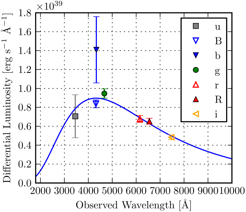
Figure 8.— SED of PTF12csy using photometry from 10 days around day 189 (observer frame) after the first detection. The fitted rest frame temperature is $T=$7160\pm 270\text{\,}\mathrm{K}$$ and the fitted bolometric luminosity $(5.53\pm 1.18)\text{\times}{10}^{42}\text{\,}\mathrm{e}\mathrm{r}\mathrm{g}\,\mathrm{s}^{-1}$.

The fit results in a reduced $\chi^{2}/n_{\text{dof}}=$7.9$/5=$1.6$$ and delivers estimates for both the rest frame temperature $T$ and the absolute bolometric luminosity $L_{\text{bol}}$ of the photosphere emitting the black body radiation: $T=$7160\pm 270\text{\,}\mathrm{K}$$ and $L_{\text{bol}}=$(5.53\pm 1.18)\text{\times}{10}^{42}\text{\,}\mathrm{e}\mathrm{r}\mathrm{g}\,\mathrm{s}^{-1}$$, where the errors correspond to . Applying the Stefan-Boltzmann law, we can calculate the radius of the black body photosphere from the bolometric luminosity. We estimate it to be $R_{\text{phot}}=$(1.7\pm 0.1)\text{\times}{10}^{15}\text{\,}\mathrm{c}\mathrm{m}$$.

Finally, to obtain an estimate on the total radiated energy, the lines’ contributions to the luminosity have to be added to the continuum luminosity. Using the Gemini North spectrum, the contribution of the H$\alpha$ and H$\beta$ line to the total luminosity is computed and added to the continuum luminosity from the black body fit. This results in an estimated total radiated luminosity of $(6.4\pm 1.2)\text{\times}{10}^{42}\text{\,}\mathrm{e}\mathrm{r}\mathrm{g}\,\mathrm{s}^{-1}$ at day 189 in the observer frame, i.e. day 177 in the rest frame.

We use the fitted shape of the $i$-band light curve (cf. Section 5.2, Fig. 7, Table 4) to extrapolate this value and find a total radiated luminosity of $\sim 9.7\text{\times}{10}^{42}\text{\,}\mathrm{e}\mathrm{r}\mathrm{g}\,\mathrm{s}^{-1}$ at $100\text{\,}\mathrm{d}$ (rest frame), as used in Section 5.2.3, and a total energy of $E_{\mathrm{bol}}=$2.1\text{\times}{10}^{50}\text{\,}\mathrm{e}\mathrm{r}\mathrm{g}$$ radiated within 400 rest frame days after first detection, comparable to SN 2008iy which had $\sim 2\text{\times}{10}^{50}\text{\,}\mathrm{e}\mathrm{r}\mathrm{g}$) (Miller et al., 2010b) and SN 2010jl with $4.3\text{\times}{10}^{50}\text{\,}\mathrm{e}\mathrm{r}\mathrm{g}$ (Zhang et al., 2012). This is a lower limit on the total radiated energy, since we lack photometric data between explosion and first detection and do not extrapolate before the first detection. Additionally, as discussed below, we are neglecting a possible contribution of X-ray and $\gamma$-ray emission to the total radiated energy, which is not considered by the black body spectrum based on the UV and optical data.

We recommend to treat these results with caution, since Ofek et al. (2014b) pointed out that at late times the fraction of energy released from SNe IIn in X-rays can increase, causing the optical spectrum to deviate from a black body as fewer photons are available in the optical. This can lead to an effective decrease of the estimated photospheric radius. In this context, our estimates of $R_{\mathrm{phot}}$, $L_{\mathrm{bol}}$, and $E_{\mathrm{bol}}$ must be treated as lower limits. Unfortunately, the X-ray flux from PTF12csy was not detected (see Section 4.2).

5.3. Spectroscopy

Two spectra were acquired (Table 5, Fig. 9). They are dominated by narrow emission lines, characteristic for Type IIn SNe, with a very weak blue continuum, which indicates the old age of the SN. No continuum is visible in the late spectrum. The SN emission lines are primarily hydrogen, the Balmer series is visible from H$\alpha$ up to H$\epsilon$. The oxygen lines O i $\lambda\lambda 7772,7774,7775,8447$, O ii $\lambda 3727$ with FWHM $\approx$500\text{\,}\mathrm{k}\mathrm{m}\,\mathrm{s}^{-1}$$, and O iii $\lambda\lambda 4364,4960,5008$ with FWHM $\approx$350\text{\,}\mathrm{k}\mathrm{m}\,\mathrm{s}^{-1}$$ are very narrow and were most likely produced by circumstellar gas released by the progenitor prior to explosion and then photoionized by UV radiation (Filippenko, 1997).

Table 5Log of spectral observations

MJD	$T_{\text{disc}}$	$T_{\text{det}}$	$\Delta v$ ($\mathrm{k}\mathrm{m}\,\mathrm{s}^{-1}$)	Instrument
56034	11	175	80	Gemini North GMOS
56332	290	454	100	Keck I LRIS

Note. — $T_{\text{disc}}$: Rest frame days after PTF discovery. $T_{\text{det}}$: Rest frame days after first detection by PS1. $\Delta v$: spectral resolution at the H$\alpha$ line at $7014\text{\,}\mathrm{\SIUnitSymbolAngstrom}$ in observer frame.

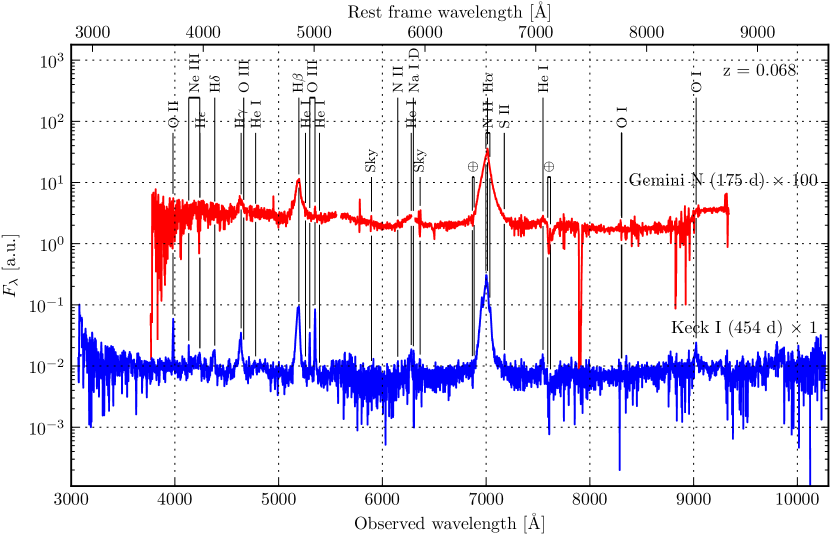
Figure 9.— Spectra taken with Gemini North on 2012 April 17 (top) and Keck I on 2013 February 09, showing narrow (Type IIn) emission lines. The H$\alpha$ line at $\sim$7000\text{\,}\mathrm{\SIUnitSymbolAngstrom}$$ (observer frame) is the strongest emission line and has a complicated structure. See Fig. 10 for a close-up of the H$\alpha$ line.

Figure 10 shows a close-up on the H$\alpha$ line from both spectra, plotted vs. Doppler velocity relative to the rest frame line center. In the early spectrum, the H$\alpha$ line peaks at the line center and the line is composed of a narrow, intermediate and broad component with FWHM of $\sim$400\text{\,}\mathrm{k}\mathrm{m}\,\mathrm{s}^{-1}$$, $\sim$2000\text{\,}\mathrm{k}\mathrm{m}\,\mathrm{s}^{-1}$$, and $\sim$5000\text{\,}\mathrm{k}\mathrm{m}\,\mathrm{s}^{-1}$$ respectively, found by fitting a superposition of three Gaussian functions to the H$\alpha$ profile. This is similar to other SNe IIn, e.g. SN 1988Z and 2008iy (Turatto et al., 1993; Filippenko, 1997; Miller et al., 2010b). The H$\alpha$ profile with broad and intermediate-width component can be explained as a result of the interaction of the SN ejecta with a two-component wind (Chugai & Danziger, 1994). In this model, the broad line component is emitted from shocked SN ejecta expanding in a relatively rarefied wind, while the intermediate component arises from a shocked dense part of the wind, which can either consist of dense clumps or be a dense equatorial wind (Chugai & Danziger, 1994). This is an indication of ejecta-CSM interaction.

The intermediate and broad component of the early spectrum’s H$\alpha$ line are blueshifted which may indicate formation of dust, as explored by Smith et al. (2012) for SN 2010jl. A more recent study by Gall et al. (2014), the most comprehensive work on the SN 2010jl emission line blueshifts to date, finds very strong evidence for a wavelength dependence of the blueshift. Therefore, the authors conclude that the origin of the blueshifts is most likely the rapid formation of large dust grains, confirming Smith et al. (2012) and having implications on the origin of dust in galaxies.

Alternatively, Fransson et al. (2014) explain the line blueshift in SN 2010jl with a bulk velocity of the emitting gas towards the observer. This is more consistent with observations if the spectral lines are symmetric about a center and if there is no wavelength dependence of the blueshift. The bulk velocity is believed to be the result of radiative acceleration of the gas by flux from the SN. Presumably, there are also other possible explanations for the blueshift, e.g. the geometry or density structure of the CSM. In case of SN PTF12csy, spectral line blueshift is only clearly visible in the H$\alpha$ line, prohibiting the interpretation of the blueshift in favor of any scenario.

The late spectrum’s H$\alpha$ line has a much more complicated structure than the early spectrum’s. It does not peak at zero velocity anymore, but the peak is blueshifted and there are many sub-peaks. Again, the blueshift might be connected to dust formation or radiative gas acceleration, but other reasons are conceivable as well. At least part of the late H$\alpha$ line’s complex appearance might be due to superposition of other spectral lines, e.g. N ii. Apart from that, it is an indication of an inhomogeneous, maybe clumpy, CSM structure, and perhaps asymmetric SN explosion.

Figure 10.— Comparison of the H$\alpha$ line in both spectra. The x-axis shows the Doppler velocity relative to the line center at $6564.61\text{\,}\mathrm{\SIUnitSymbolAngstrom}$, assuming a redshift of 0.0684.

The spectra are compared to template spectra from the Padova-Asiago Supernova Archive (ASA) (Harutyunyan et al., 2008) using the online tool GELATO. The algorithm (Harutyunyan et al., 2008) divides a spectrum into 11 relevant bins and averages within the bins to classify and compare with the archived spectra. The PTF12csy spectra are de-reddened with $E(B-V)=0.1$ and compared to other Type II SNe. GELATO returns the best 30 matching spectra together with their phases, ordered by quality of fit. For both the Gemini North spectrum taken at $175\text{\,}\mathrm{d}$ and the Keck I spectrum from $454\text{\,}\mathrm{d}$, the majority of best matching template spectra come from SN 2010jl. The mean phase of the matching spectra is significantly higher for the Keck I spectrum: $378\pm 102\text{\,}\mathrm{d}$, versus $154\pm 21\text{\,}\mathrm{d}$ for the Gemini N spectrum. However, the reference dates for the spectra are mostly the discovery date, only rarely the date of maximum light or explosion date.

5.4. Host Galaxy

The galaxy hosting PTF12csy is a faint dwarf galaxy designated SDSS J065832.82+171541.6, barely visible in the SDSS DR12 images. Since it has no cataloged redshift, we measure its redshift via O ii $\lambda 3727$ and O iii $\lambda\lambda 4960,5008$ lines in the Keck I spectrum. The redshift is $0.0684\pm 0.0001$, corresponding to a luminosity distance of $\sim 300\text{\,}\mathrm{M}\mathrm{p}\mathrm{c}$ assuming standard cosmology with Hubble parameter $H_{0}=$70\text{\,}\mathrm{k}\mathrm{m}\,\mathrm{s}^{-1}\,\mathrm{M}\mathrm{p}\mathrm{c}^{-1}$$, matter density $\Omega_{m}=0.3$, and dark energy density $\Omega_{\Lambda}=0.7$.

Adopting the luminosity distance from above, the host galaxy has absolute magnitudes of $M_{g}\approx$-16.2\text{\,}\mathrm{m}\mathrm{a}\mathrm{g}$$, $M_{r}\approx$-16.6\text{\,}\mathrm{m}\mathrm{a}\mathrm{g}$$ and $M_{i}\approx$-16.7\text{\,}\mathrm{m}\mathrm{a}\mathrm{g}$$ (corrected for Galactic extinction). Using the luminosity-metallicity relation from Lee et al. (2006, eq. 1), we find a metallicity of $12+\log{\text{O}/\text{H}}\approx 8$, indicating that the host galaxy is quite metal-poor. Overluminous SNe IIn, such as PTF12csy, have been preferentially found to occur in subluminous, low-metallicity galaxies (Miller et al., 2010b; Stoll et al., 2011), such as the host of PTF12csy. This is a trend, which is also observed for long GRBs (Stoll et al., 2011). Statistics are still low and Miller et al. (2010b) cautioned that there could be some selection bias due to intrinsically bright SNe in faint host galaxies being more easily discovered during surveys doing aperture photometry. However, new surveys performing image subtraction and observing large untargeted fields, e.g. PTF and Pan-STARRS, provide increasing evidence for this trend, as most of the discovered bright objects would have been luminous enough to be detected in bright galaxies and in searches that are targeted to bright galaxies (Stoll et al., 2011). PTF12csy, probably discovered by coincidence in an unbiased way, confirms this emerging trend as well.

The SDSS DR12 has the host galaxy’s cataloged center position about $3\text{\,}\arcsec$ away from the found SN position (see also Fig. 2). With an apparent diameter of about $5\text{\,}\arcsec$, corresponding to $\sim$7\text{\,}\mathrm{k}\mathrm{p}\mathrm{c}$$, this is quite far from the center of the galaxy, i.e. about $4\text{\,}\mathrm{k}\mathrm{p}\mathrm{c}$ off-center.

6. SUMMARY AND CONCLUSION

The highest significance alert from the IceCube Optical Follow-Up program led to a coincidental discovery of the interesting and unusual Type IIn SN PTF12csy, which was already at least 169 days old. The combined a posteriori significance of the neutrino doublet alert and the coincident detection of any core-collapse SN within the error radius of the neutrino events ($0.54\text{\,}\mathrm{\SIUnitSymbolDegree}$) and within the luminosity distance of the SN ($300\text{\,}\mathrm{M}\mathrm{p}\mathrm{c}$) is , for the time interval of the IceCube data acquisition season 2011/12.

PTF12csy is rare and unusual: With peak absolute magnitudes of $M_{r}<-19$, perhaps about -20, it belongs to the most luminous SNe. The SN is most likely powered by interaction of the ejecta with a dense circumstellar medium (CSM). The spectrum indicates a complicated structure of the CSM. Its host galaxy is a faint and metal-poor dwarf galaxy, confirming an observed trend for luminous SNe IIn. PTF12csy is similar in photometry and spectroscopy to other rare luminous SNe IIn, e.g. SNe 2008iy and 2010jl. The total radiated energy is $2\text{\times}{10}^{50}\text{\,}\mathrm{e}\mathrm{r}\mathrm{g}$ within the first 400 rest frame days after detection.

Given the ejecta-CSM interaction, high-energy (HE) cosmic ray production and neutrino emission may be expected on a time scale of $110\text{\,}\mathrm{m}\mathrm{o}\mathrm{n}\mathrm{t}\mathrm{h}\mathrm{s}$, according to Murase et al. (2011) and Katz et al. (2012). However, the SN is too far away for IceCube to detect this emission. A complementary neutrino analysis performed offline, using one year of IceCube data which cover most of the optical SN fluence, does not reveal a signal-like accumulation of neutrino events from the SN’s position, leading to a very high upper limit of more than 1000 times the tested model fluence, owing to the large distance.

Due to the long delay of several months between explosion date and neutrinos, the doublet of neutrinos within less than two seconds cannot be explained by the formation of a jet shortly after core-collapse according to the choked jet model (Ando & Beacom, 2005). Nor can it be explained by the expected HE neutrino production from ejecta-CSM interaction of SNe IIn (s.a.). We therefore conclude that the only reasonable explanation is that the SN detection was coincidental and the neutrino doublet was produced by uncorrelated background events of atmospheric neutrinos and/or mis-reconstructed atmospheric muons.

However, if there was a delaying mechanism at work, such as the spin-down of a supramassive neutron star that delays its collapse to a black hole, as in the blitzar model (Falcke & Rezzolla, 2014), then the neutrino doublet may have originated from a jet forming in the course of this delayed collapse few hundred days after SN explosion.

The coincidental detection of a Type IIn SN following an IceCube neutrino alert demonstrates the capability of the follow-up system to reveal transient HE neutrino sources. An advantage of the follow-up paradigm is the prompt availability of multi-messenger information for the identification of the source, as well as the mere statistical significance of a coincidence between a neutrino burst and an electromagnetic transient detection. In this case, the significance is very low due to the delay of several months between explosion and neutrinos. However, this coincidence motivates the continuation of the follow-up program as well as further stacked neutrino analyses of Type IIn supernovae.

References

- Aartsen et al. (2013) Aartsen, M. G., Abbasi, R., Abdou, Y., et al. 2013, arXiv:1309.6979
- Aartsen et al. (2014) Aartsen, M. G., Abbasi, R., Ackermann, M., et al. 2014, Journal of Instrumentation, 9, 3009P
- Aartsen et al. (2014a) Aartsen, M. G., Ackermann, M., Adams, J., et al. 2014a, Phys. Rev. Lett., 113, 101101
- Aartsen et al. (2014b) —. 2014b, ApJ, 796, 109
- Abbasi et al. (2012) Abbasi, R., Abdou, Y., Abu-Zayyad, T., et al. 2012, A&A, 539, A60
- Achterberg et al. (2006) Achterberg, A., Ackermann, M., Adams, J., et al. 2006, APh, 26, 155
- Ahn et al. (2014) Ahn, C. P., Alexandroff, R., Allende Prieto, C., et al. 2014, ApJS, 211, 17
- Ahrens et al. (2004) Ahrens, J., Bai, X., Bay, R., et al. 2004, Nuclear Instruments and Methods in Physics Research A, 524, 169
- Akerlof et al. (2003) Akerlof, C. W., Kehoe, R. L., McKay, T. A., et al. 2003, PASP, 115, pp. 132
- Alam et al. (2015) Alam, S., Albareti, F. D., Allende Prieto, C., et al. 2015, arXiv:1501.00963
- Ando & Beacom (2005) Ando, S., & Beacom, J. F. 2005, Phys. Rev. Lett., 95, 061103
- Baret et al. (2011) Baret, B., Bartos, I., Bouhou, B., et al. 2011, APh, 35, 1
- Becker et al. (2006) Becker, J. K., Stamatikos, M., Halzen, F., & Rhode, W. 2006, APh, 25, 118
- Blaufuss (2013) Blaufuss, E. 2013, GCN Circular 14520 13/05/01
- Braun et al. (2010) Braun, J., Baker, M., Dumm, J., et al. 2010, APh, 33, 175
- Braun et al. (2008) Braun, J., Dumm, J., De Palma, F., et al. 2008, APh, 29, 299
- Brown (1975) Brown, M. B. 1975, Biometrics, 31, pp. 987
- Brown et al. (2013) Brown, T. M., Baliber, N., Bianco, F. B., et al. 2013, PASP, 125, 1031
- Cardelli et al. (1989) Cardelli, J. A., Clayton, G. C., & Mathis, J. S. 1989, ApJ, 345, 245
- Chevalier (1982) Chevalier, R. A. 1982, ApJ, 259, 302
- Chugai & Danziger (1994) Chugai, N. N., & Danziger, I. J. 1994, MNRAS, 268, 173
- Cowen et al. (2010) Cowen, D. F., Franckowiak, A., & Kowalski, M. 2010, APh, 33, 19
- Drake et al. (2010) Drake, A. J., Djorgovski, S. G., Prieto, J. L., et al. 2010, ApJ, 718, L127
- Eisenstein et al. (2011) Eisenstein, D. J., Weinberg, D. H., Agol, E., et al. 2011, AJ, 142, 72
- Evans et al. (2014) Evans, P. A., Osborne, J. P., Beardmore, A. P., et al. 2014, ApJS, 210, 8
- Evans et al. (2015) Evans, P. A., Osborne, J. P., Kennea, J. A., et al. 2015, MNRAS, 448, 2210
- Falcke & Rezzolla (2014) Falcke, H., & Rezzolla, L. 2014, A&A, 562, A137
- Filippenko (1997) Filippenko, A. V. 1997, ARA&A, 35, 309
- Fisher (1950) Fisher, R. 1950, Statistical Methods for Research Workers, Eleventh Edition, Revised, [Biological Monographs and Manuals. no. 5.] (Edinburgh, London: Oliver and Boyd), 99–101
- Fisher (1990) Fisher, R. A. 1990, Statistical Methods, Experimental Design, and Scientific Inference: A Re-issue of Statistical Methods for Research Workers, The Design of Experiments, and Statistical Methods and Scientific Inference (Oxford England New York: Oxford University Press)
- Fransson et al. (2014) Fransson, C., Ergon, M., Challis, P. J., et al. 2014, ApJ, 797, 118
- Fukugita et al. (1996) Fukugita, M., Ichikawa, T., Gunn, J. E., et al. 1996, AJ, 111, 1748
- Gal-Yam (2012) Gal-Yam, A. 2012, Sci, 337, 927
- Gall et al. (2014) Gall, C., Hjorth, J., Watson, D., et al. 2014, Nature, 511, 32
- Gehrels et al. (2004) Gehrels, N., Chincarini, G., Giommi, P., et al. 2004, ApJ, 611, 1005
- Gunn et al. (2006) Gunn, J. E., Siegmund, W. A., Mannery, E. J., et al. 2006, AJ, 131, 2332
- Harutyunyan et al. (2008) Harutyunyan, A. H., Pfahler, P., Pastorello, A., et al. 2008, A&A, 488, 383
- Hook et al. (2004) Hook, I. M., Jørgensen, I., Allington-Smith, J. R., et al. 2004, PASP, 116, 425
- Horiuchi et al. (2013) Horiuchi, S., Beacom, J. F., Bothwell, M. S., & Thompson, T. A. 2013, ApJ, 769, 113
- Kaiser (2004) Kaiser, N. 2004, Proc. SPIE, 5489, 11
- Katz et al. (2012) Katz, B., Sapir, N., & Waxman, E. 2012, in IAU Symposium, Vol. 279, Death of Massive Stars: Supernovae and Gamma-Ray Bursts, 274–281
- Kawabata et al. (2009) Kawabata, K. S., Tanaka, M., Maeda, K., et al. 2009, ApJ, 697, 747
- Kelner et al. (2006) Kelner, S. R., Aharonian, F. A., & Bugayov, V. V. 2006, Phys. Rev. D, 74, 034018
- Kowalski & Mohr (2007) Kowalski, M., & Mohr, A. 2007, APh, 27, 533
- Kraft et al. (1991) Kraft, R. P., Burrows, D. N., & Nousek, J. A. 1991, ApJ, 374, 344
- Kulkarni (2005) Kulkarni, S. R. 2005, arXiv:astro-ph/0510256
- Laher et al. (2014) Laher, R. R., Surace, J., Grillmair, C. J., et al. 2014, PASP, 126, pp. 674
- Law et al. (2009) Law, N., Kulkarni, S., Dekany, R., et al. 2009, PASP, 121, pp. 1395
- Lee et al. (2006) Lee, H., Skillman, E. D., Cannon, J. M., et al. 2006, ApJ, 647, 970
- Lien et al. (2014) Lien, A., Sakamoto, T., Gehrels, N., et al. 2014, ApJ, 783, 24
- Littell & Folks (1971) Littell, R. C., & Folks, J. L. 1971, Journal of the American Statistical Association, 66, pp. 802
- Magnier (2006) Magnier, E. 2006, in The Advanced Maui Optical and Space Surveillance Technologies Conference, 50
- Magnier et al. (2013) Magnier, E. A., Schlafly, E., Finkbeiner, D., et al. 2013, ApJS, 205, 20
- Margutti et al. (2014) Margutti, R., Milisavljevic, D., Soderberg, A., et al. 2014, ApJ, 780, 21
- Meszaros (2006) Meszaros, P. 2006, RPPh, 69, 2259
- Miller et al. (2010a) Miller, A. A., Smith, N., Li, W., et al. 2010a, AJ, 139, 2218
- Miller et al. (2010b) Miller, A. A., Silverman, J. M., Butler, N. R., et al. 2010b, MNRAS, 404, 305
- Moriya et al. (2013) Moriya, T. J., Maeda, K., Taddia, F., et al. 2013, MNRAS, 435, 1520
- Moriya & Tominaga (2012) Moriya, T. J., & Tominaga, N. 2012, ApJ, 747, 118
- Murase (2008) Murase, K. 2008, Phys. Rev. D, 78, 101302
- Murase et al. (2006) Murase, K., Ioka, K., Nagataki, S., & Nakamura, T. 2006, ApJ, 651, L5
- Murase & Nagataki (2006) Murase, K., & Nagataki, S. 2006, Phys. Rev. D, 73, 063002
- Murase et al. (2011) Murase, K., Thompson, T. A., Lacki, B. C., & Beacom, J. F. 2011, Phys. Rev. D, 84, 043003
- Murase et al. (2014) Murase, K., Thompson, T. A., & Ofek, E. O. 2014, MNRAS, 440, 2528
- Nasa High Energy Astrophysics Science Archive Research Center (2014) (Heasarc) Nasa High Energy Astrophysics Science Archive Research Center (Heasarc). 2014, HEAsoft: Unified Release of FTOOLS and XANADU, Astrophysics Source Code Library, ascl:1408.004
- Neunhöffer (2006) Neunhöffer, T. 2006, APh, 25, 220
- Neyman (1937) Neyman, J. 1937, RSPTA, 236, 333
- Neyman (1967) —. 1967, A Selection of Early Statistical Papers of J. Neyman, The Selected Papers of Jerzy Neyman and E. S. Pearson (University of California Press)
- Ofek et al. (2014a) Ofek, E. O., Sullivan, M., Shaviv, N. J., et al. 2014a, ApJ, 789, 104
- Ofek et al. (2007) Ofek, E. O., Cameron, P. B., Kasliwal, M. M., et al. 2007, ApJ, 659, L13
- Ofek et al. (2012) Ofek, E. O., Laher, R., Law, N., et al. 2012, PASP, 124, 62
- Ofek et al. (2013) Ofek, E. O., Fox, D., Cenko, S. B., et al. 2013, ApJ, 763, 42
- Ofek et al. (2014b) Ofek, E. O., Zoglauer, A., Boggs, S. E., et al. 2014b, ApJ, 781, 42
- Oke et al. (1995) Oke, J. B., Cohen, J. G., Carr, M., et al. 1995, PASP, 107, 375
- Pejcha & Thompson (2015) Pejcha, O., & Thompson, T. A. 2015, ApJ, 801, 90
- Rau et al. (2009) Rau, A., Kulkarni, S. R., Law, N. M., et al. 2009, PASP, 121, pp. 1334
- Razzaque et al. (2004) Razzaque, S., Mészáros, P., & Waxman, E. 2004, Phys. Rev. Lett., 93, 181101
- Richardson et al. (2002) Richardson, D., Branch, D., Casebeer, D., et al. 2002, AJ, 123, 745
- Schlegel et al. (1998) Schlegel, D. J., Finkbeiner, D. P., & Davis, M. 1998, ApJ, 500, 525
- Schlegel (1990) Schlegel, E. M. 1990, MNRAS, 244, 269
- Smith et al. (2012) Smith, N., Silverman, J. M., Filippenko, A. V., et al. 2012, AJ, 143, 17
- Smith et al. (2007) Smith, N., Li, W., Foley, R. J., et al. 2007, ApJ, 666, 1116
- Stoll et al. (2011) Stoll, R., Prieto, J. L., Stanek, K. Z., et al. 2011, ApJ, 730, 34
- Svirski et al. (2012) Svirski, G., Nakar, E., & Sari, R. 2012, ApJ, 759, 108
- Tonry et al. (2012) Tonry, J. L., Stubbs, C. W., Lykke, K. R., et al. 2012, ApJ, 750, 99
- Turatto et al. (1993) Turatto, M., Cappellaro, E., Danziger, I. J., et al. 1993, MNRAS, 262, 128
- Waxman & Bahcall (1997) Waxman, E., & Bahcall, J. 1997, Phys. Rev. Lett., 78, 2292
- Willingale et al. (2013) Willingale, R., Starling, R. L. C., Beardmore, A. P., Tanvir, N. R., & O’Brien, P. T. 2013, MNRAS, 431, 394
- Yaron & Gal-Yam (2012) Yaron, O., & Gal-Yam, A. 2012, PASP, 124, 668
- Zhang et al. (2012) Zhang, T., Wang, X., Wu, C., et al. 2012, AJ, 144, 131