Provable Bayesian Inference via Particle Mirror Descent

Bo Dai1 Niao He2 Hanjun Dai1 Le Song1
1 Georgia Institute of Technology
{bodai
hanjundai}@gatech.edu lsong@cc.gatech.edu
2 University of Illinois at Urbana-Champaign
niaohe@illinois.edu
Abstract

Bayesian methods are appealing in their flexibility in modeling complex data and ability in capturing uncertainty in parameters. However, when Bayes’ rule does not result in tractable closed-form, most approximate inference algorithms lack either scalability or rigorous guarantees. To tackle this challenge, we propose a simple yet provable algorithm, Particle Mirror Descent (PMD), to iteratively approximate the posterior density. PMD is inspired by stochastic functional mirror descent where one descends in the density space using a small batch of data points at each iteration, and by particle filtering where one uses samples to approximate a function. We prove result of the first kind that, with m𝑚m particles, PMD provides a posterior density estimator that converges in terms of KL𝐾𝐿KL-divergence to the true posterior in rate O(1/m)𝑂1𝑚O(1/\sqrt{m}). We demonstrate competitive empirical performances of PMD compared to several approximate inference algorithms in mixture models, logistic regression, sparse Gaussian processes and latent Dirichlet allocation on large scale datasets.

1 Introduction

Bayesian methods are attractive because of their ability in modeling complex data and capturing uncertainty in parameters. The crux of Bayesian inference is to compute the posterior distribution, p(θ|X)p(θ)n=1Np(xn|θ)proportional-to𝑝conditional𝜃𝑋𝑝𝜃superscriptsubscriptproduct𝑛1𝑁𝑝conditionalsubscript𝑥𝑛𝜃p(\theta|X)\propto p(\theta)\prod\nolimits_{n=1}^{N}p(x_{n}|\theta), of a parameter θd𝜃superscript𝑑\theta\in\mathbb{R}^{d} given a set of N𝑁N data points X={xn}n=1N𝑋superscriptsubscriptsubscript𝑥𝑛𝑛1𝑁X=\left\{x_{n}\right\}_{n=1}^{N} from Dsuperscript𝐷\mathbb{R}^{D}, with a prior distribution p(θ)𝑝𝜃p(\theta) and a model of data likelihood p(x|θ)𝑝conditional𝑥𝜃p(x|\theta). For many non-trivial models from real-world applications, the prior might not be conjugate to the likelihood or might contain hierarchical structure. Therefore, computing the posterior often results in intractable integration and poses computational challenges. Typically, one resorts to approximate inference such as sampling, e.g., MCMC [31] and SMC [14], or variational inference [24, 40].

Two longstanding challenges in approximate Bayesian inference are i) provable convergence and ii) data-intensive computation at each iteration. MCMC is a general algorithm known to generate samples from distribution that converges to the true posterior. However, in order to generate a single sample at every iteration, it requires a complete scan of the dataset and evaluation of the likelihood at each data point, which is computationally expensive. To address this issue, approximate sampling algorithms have been proposed which use only a small batch of data points at each iteration [e.g. 8, 3, 42, 26]. Chopin [8], Balakrishnan and Madigan [3] extend the sequential Monte Carlo (SMC) to Bayesian inference on static models. However, these algorithms rely on Gaussian distribution or kernel density estimator as transition kernel for efficiency, which breaks down the convergence guarantee of SMC. On the other hand, the stochastic Langevin dynamics algorithm (SGLD) [42] and its derivatives [2, 7, 13] combine ideas from stochastic optimization and Hamiltonian Monte Carlo, and are proven to converge in terms of integral approximation, as recently shown in [39, 36]. Still, it is unclear whether the dependent samples generated reflects convergence to the true posterior. FireflyMC [26], introduces auxiliary variables to switch on and off data points to save computation for likelihood evaluations, but this algorithm requires the knowledge of lower bounds of likelihood that is model-specific and may be hard to calculate.

In another line of research, the variational inference algorithms [24, 40, 28] attempt to approximate the entire posterior density by optimizing information divergence [29]. The recent derivatives [19] avoid examination of all the data in each update. However, the major issue for these algorithms is the absence of theoretical guarantees. This is due largely to the fact that variational inference algorithms typically choose a parametric family to approximate the posterior density, which can be far from the true posterior, and require to solve a highly non-convex optimization problem. In most cases, these algorithms optimize over simple exponential family for tractability. More flexible variational families have been explored but largely restricted to mixture models [23, 15]. In these cases, it is often difficult to quantify the approximation and optimization error at each iteration, and analyze how the error accumulates across the iterations. Therefore, a provably convergent variational inference algorithm is still needed.

In this paper, we present such a simple and provable nonparametric inference algorithm, Particle Mirror Descent (PMD), to iteratively approximate the posterior density. PMD relies on the connection that Bayes’ rule can be expressed as the solution to a convex optimization problem over the density space [43, 44, 45]. However, directly solving the optimization will lead to both computational and representational issues: one scan over the entire dataset at each iteration is needed, and the exact function update has no closed-form. To address these issues, we draw inspiration from two sources: (i) stochastic mirror descent, where one can instead descend in the density space using a small batch of data points at each iteration; and (ii) particle filtering and kernel density estimation, where one can maintain a tractable approximate representation of the density using samples. In summary, PMD possesses a number of desiderata:

Simplicity. PMD applies to many probabilistic models, even with non-conjugate priors. The algorithm is summarized in just a few lines of codes, and only requires the value of likelihood and prior, unlike other approximate inference techniques [42, 15, 33, 19, e.g.], which typically require their first and/or second-order derivatives.

Flexibility. Different from other variational inference algorithms, which sacrifice the model flexibility for tractability, our method approximates the posterior by particles or kernel density estimator. The flexibility of nonparametric model enables PMD to capture multi-modal in posterior.

Stochasticity. At iteration t𝑡t, PMD only visits a mini-batch of data to compute the stochastic functional gradient, and samples O(t)𝑂𝑡O(t) points from the solution. Hence, it avoids scanning over the whole dataset in each update.

Theoretical guarantees. We show the density estimator provided by PMD converges in terms of both integral approximation and KL𝐾𝐿KL-divergence to the true posterior density in rate O(1/m)𝑂1𝑚O(1/\sqrt{m}) with m𝑚m particles. To our best knowledge, these results are the first of the kind in Bayesian inference for estimating posterior.

In the remainder, we will introduce the optimization view of Bayes’ rule before presenting our algorithm, and then we provide both theoretical and empirical supports of PMD.

Throughout this paper, we denote KL𝐾𝐿KL as the Kullback-Leibler divergence, function q(θ)𝑞𝜃q(\theta) as q𝑞q, a random sequence as θ[t]:=[θ1,,θt]assignsubscript𝜃delimited-[]𝑡subscript𝜃1subscript𝜃𝑡\theta_{[t]}:=[\theta_{1},\ldots,\theta_{t}], integral f()𝑓f(\cdot) w.r.t. some measure μ(θ)𝜇𝜃\mu(\theta) over support ΩΩ\Omega as f(θ)μ(dθ)𝑓𝜃𝜇𝑑𝜃\int f(\theta)\mu(d\theta), or f(θ)𝑑θ𝑓𝜃differential-d𝜃\int f(\theta)d\theta without ambiguity, ,L2subscriptsubscript𝐿2\langle\cdot,\cdot\rangle_{L_{2}} as the L2subscript𝐿2L_{2} inner product, and p\|\cdot\|_{p} as the Lpsubscript𝐿𝑝L_{p} norm for 1p1𝑝1\leqslant p\leqslant\infty.

2 Optimization View of Bayesian Inference

Our algorithm stems from the connection between Bayes’ rule and optimization. Williams [43], Zellner [44], Zhu et al. [45] showed that Bayes’ rule

p(θ|X)=p(θ)n=1Np(xn|θ)p(X)𝑝conditional𝜃𝑋𝑝𝜃superscriptsubscriptproduct𝑛1𝑁𝑝conditionalsubscript𝑥𝑛𝜃𝑝𝑋p(\theta|{X})=\frac{p(\theta)\prod_{n=1}^{N}p({x}_{n}|\theta)}{p({X})}

where p(X)=p(θ)n=1Np(xn|θ)dθ𝑝𝑋𝑝𝜃superscriptsubscriptproduct𝑛1𝑁𝑝conditionalsubscript𝑥𝑛𝜃𝑑𝜃p({X})=\int p(\theta)\prod_{n=1}^{N}p({x}_{n}|\theta)d\theta, can be obtained by solving the optimization problem

minq(θ)𝒫L(q):=n=1N[q(θ)logp(xn|θ)dθ]+KL(q(θ)||p(θ)),\displaystyle\min_{q(\theta)\in\mathcal{P}}L(q):=-\sum_{n=1}^{N}\bigg{[}\int q(\theta)\log p({x}_{n}|\theta)\,d\theta\bigg{]}+KL(q(\theta)\,||\,p(\theta)), (1)

where 𝒫𝒫\mathcal{P} is the valid density space. The objective, L(q)𝐿𝑞L(q), is continuously differentiable with respect to q𝒫𝑞𝒫q\in\mathcal{P} and one can further show that

Lemma 1

Objective function L(q)𝐿𝑞L(q) defined on q(θ)𝒫𝑞𝜃𝒫q(\theta)\in\mathcal{P} is 111-strongly convex w.r.t. KL𝐾𝐿KL-divergence.

Despite of the closed-form representation of the optimal solution, it can be challenging to compactly represent, tractably compute, or efficiently sample from the solution. The normalization, p(X)=p(θ)n=1Np(xn|θ)dθ𝑝𝑋𝑝𝜃superscriptsubscriptproduct𝑛1𝑁𝑝conditionalsubscript𝑥𝑛𝜃𝑑𝜃p({X})=\int p(\theta)\prod_{n=1}^{N}p({x}_{n}|\theta)d\theta, involves high dimensional integral and typically does not admit tractable closed-form computation. Meanwhile, the product in the numerator could be arbitrarily complicated, making it difficult to represent and sample from. However, this optimization perspective provides us a way to tackle these challenges by leveraging recent advances from optimization algorithms.

2.1 Stochastic Mirror Descent in Density Space

We will resort to stochastic optimization to avoid scanning the entire dataset for each gradient evaluation. The stochastic mirror descent [32] expands the usual stochastic gradient descent scheme to problems with non-Euclidean geometries, by applying unbiased stochastic subgradients and Bregman distances as prox-map functions. We now explain in details, the stochastic mirror descent algorithm in the context of Bayesian inference.

At t𝑡t-th iteration, given a data point xtsubscript𝑥𝑡x_{t} drawn randomly from the dataset, the stochastic functional gradient of L(q)𝐿𝑞L(q) with respect to q(θ)L2𝑞𝜃subscript𝐿2q(\theta)\in L_{2} is gt(θ)=log(q(θ))log(p(θ))Nlogp(xt|θ)subscript𝑔𝑡𝜃𝑞𝜃𝑝𝜃𝑁𝑝conditionalsubscript𝑥𝑡𝜃g_{t}(\theta)=\log(q(\theta))-\log(p(\theta))-N\log p(x_{t}|\theta). The stochastic mirror descent iterates over the prox-mapping step qt+1=𝐏qt(γtgt)subscript𝑞𝑡1subscript𝐏subscript𝑞𝑡subscript𝛾𝑡subscript𝑔𝑡q_{t+1}=\mathbf{P}_{q_{t}}(\gamma_{t}g_{t}), where γt>0subscript𝛾𝑡0\gamma_{t}>0 is the stepsize and

𝐏q(g):=argminq^(θ)𝒫{q^,gL2+KL(q^q)}.assignsubscript𝐏𝑞𝑔subscriptargmin^𝑞𝜃𝒫subscript^𝑞𝑔subscript𝐿2𝐾𝐿conditional^𝑞𝑞\displaystyle\mathbf{P}_{q}(g):=\mathop{\mathrm{argmin}}\nolimits_{\widehat{q}(\theta)\in\mathcal{P}}\,\{\left\langle\widehat{q},g\right\rangle_{L_{2}}+KL(\widehat{q}\|q)\}.

Since the domain is density space, KL𝐾𝐿KL-divergence is a natural choice for the prox-function. The prox-mapping therefore admits the closed-form

qt+1(θ)subscript𝑞𝑡1𝜃\displaystyle q_{t+1}(\theta) =\displaystyle= qt(θ)exp(γtgt(θ))/Zsubscript𝑞𝑡𝜃subscript𝛾𝑡subscript𝑔𝑡𝜃𝑍\displaystyle q_{t}(\theta)\exp(-\gamma_{t}g_{t}(\theta))/Z
=\displaystyle= qt(θ)1γtp(θ)γtp(xt|θ)Nγt/Z,subscript𝑞𝑡superscript𝜃1subscript𝛾𝑡𝑝superscript𝜃subscript𝛾𝑡𝑝superscriptconditionalsubscript𝑥𝑡𝜃𝑁subscript𝛾𝑡𝑍\displaystyle q_{t}(\theta)^{1-\gamma_{t}}p(\theta)^{\gamma_{t}}p(x_{t}|\theta)^{N\gamma_{t}}/Z,

where Z:=qt(θ)exp(γtgt(θ))𝑑θassign𝑍subscript𝑞𝑡𝜃subscript𝛾𝑡subscript𝑔𝑡𝜃differential-d𝜃Z:=\int q_{t}(\theta)\exp(-\gamma_{t}g_{t}(\theta))\,d\theta is the normalization. This update is similar the Bayes’ rule. However, an important difference here is that the posterior is updated using the fractional power of the previous solution, the prior and the likelihood. Still computing qt+1(θ)subscript𝑞𝑡1𝜃q_{t+1}(\theta) can be intractable due to the normalization Z𝑍Z.

2.2 Error Tolerant Stochastic Mirror Descent

To handle the intractable integral normalization at each prox-mapping step, we will consider a modified version of the stochastic mirror descent algorithm which can tolerate additional error in the prox-mapping step. Given ϵ0italic-ϵ0\epsilon\geqslant 0 and gL2𝑔subscript𝐿2g\in L_{2}, we define the ϵitalic-ϵ\epsilon-prox-mapping of q𝑞q as the set

𝐏qϵ(g):={q^𝒫:KL(q^||q)+g,q^L2minq^𝒫{KL(q^||q)+g,q^L2}+ϵ},\displaystyle\mathbf{P}_{q}^{\epsilon}(g):=\{\widehat{q}\in\mathcal{P}\,:\,KL(\widehat{q}||q)+\langle g,\widehat{q}\rangle_{L_{2}}\leqslant\min\nolimits_{\widehat{q}\in\mathcal{P}}\{KL(\widehat{q}||q)+\langle g,\widehat{q}\rangle_{L_{2}}\}+\epsilon\}, (3)

and consider the update q~t+1(θ)𝐏q~tϵt(γtgt)subscript~𝑞𝑡1𝜃superscriptsubscript𝐏subscript~𝑞𝑡subscriptitalic-ϵ𝑡subscript𝛾𝑡subscript𝑔𝑡\tilde{q}_{t+1}(\theta)\in\mathbf{P}_{\tilde{q}_{t}}^{\epsilon_{t}}(\gamma_{t}g_{t}). When ϵt=0,tsubscriptitalic-ϵ𝑡0for-all𝑡\epsilon_{t}=0,\forall t, this reduces to the usual stochastic mirror descent algorithm. The classical results regarding the convergence rate can also be extended as below

Theorem 2

Let q=argminq𝒫L(q)superscript𝑞subscriptargmin𝑞𝒫𝐿𝑞q^{*}=\mathop{\mathrm{argmin}}_{q\in\mathcal{P}}L(q), stochastic mirror descent with inexact prox-mapping after T𝑇T steps gives the recurrence:

𝔼[KL(q||q~t+1)]ϵt+(1γt)𝔼[KL(q||q~t)]+γt22𝔼gt2\mathbb{E}[KL(q^{*}||\tilde{q}_{t+1})]\leqslant\epsilon_{t}+(1-\gamma_{t})\mathbb{E}[KL(q^{*}||\tilde{q}_{t})]+\frac{\gamma_{t}^{2}}{2}\mathbb{E}\|g_{t}\|^{2}_{\infty}

Remark 1: As shown in the classical analysis of stochastic mirror descent, we could also provide a non-asymptotic convergence results in terms of objective error at average solutions, e.g., simple average q¯T=t=1Tγtq~t/t=1Tγtsubscript¯𝑞𝑇superscriptsubscript𝑡1𝑇subscript𝛾𝑡subscript~𝑞𝑡superscriptsubscript𝑡1𝑇subscript𝛾𝑡\bar{q}_{T}=\sum_{t=1}^{T}\gamma_{t}\tilde{q}_{t}/\sum_{t=1}^{T}\gamma_{t} in Appendix B.

Remark 2: For simplicity, we present the algorithm with stochastic gradient estimated by a single data point. The mini-batch trick is also applicable to reduce the variance of stochastic gradient, and convergence remains the same order but with an improved constant.

Allowing error in each step gives us room to design more flexible algorithms. Essentially, this implies that we can approximate the intermediate density by some tractable representation. As long as the approximation error is not too large, the algorithm will still converge; and if the approximation does not involve costly computation, the overall algorithm will still be efficient.

3 Particle Mirror Descent Algorithm

We introduce two efficient strategies to approximate prox-mappings, one based on weighted particles and the other based on weighted kernel density estimator. The first strategy is designed for the situation when the prior is a “good” guess of the true posterior, while the second strategy works for general situations. Interestingly, these two methods resemble particle reweighting and rejuvenation respectively in sequential Monte Carlo yet with notable differences.

3.1 Posterior Approximation Using Weighted Particle

We first consider the situation when we are given a “good” prior, such that p(θ)𝑝𝜃p(\theta) has the same support as the true posterior q(θ)superscript𝑞𝜃q^{*}(\theta), i.e., 0q(θ)/p(θ)C0superscript𝑞𝜃𝑝𝜃𝐶0\leqslant q^{*}(\theta)/p(\theta)\leqslant C. We will simply maintain a set of samples (or particles) from p(θ)𝑝𝜃p(\theta), and utlize them to estimate the intermediate prox-mappings. Let {θi}i=1mp(θ)similar-tosuperscriptsubscriptsubscript𝜃𝑖𝑖1𝑚𝑝𝜃\left\{\theta_{i}\right\}_{i=1}^{m}\sim p(\theta) be a set of fixed i.i.d. samples. We approximate qt+1(θ)subscript𝑞𝑡1𝜃q_{t+1}(\theta) as a set of weighted particles

q~t+1(θ)=i=1mαit+1δ(θi),subscript~𝑞𝑡1𝜃superscriptsubscript𝑖1𝑚subscriptsuperscript𝛼𝑡1𝑖𝛿subscript𝜃𝑖\displaystyle\tilde{q}_{t+1}(\theta)=\sum\nolimits_{i=1}^{m}\alpha^{t+1}_{i}\,\delta(\theta_{i}), (4)
αit+1:=αitexp(γtgt(θi))i=1mαitexp(γtgt(θi)),t1.formulae-sequenceassignsubscriptsuperscript𝛼𝑡1𝑖subscriptsuperscript𝛼𝑡𝑖subscript𝛾𝑡subscript𝑔𝑡subscript𝜃𝑖superscriptsubscript𝑖1𝑚subscriptsuperscript𝛼𝑡𝑖subscript𝛾𝑡subscript𝑔𝑡subscript𝜃𝑖for-all𝑡1\displaystyle\alpha^{t+1}_{i}:=\frac{\alpha^{t}_{i}\exp(-\gamma_{t}g_{t}(\theta_{i}))}{\sum_{i=1}^{m}\alpha^{t}_{i}\exp(-\gamma_{t}g_{t}(\theta_{i}))},\forall t\geqslant 1.

The update is derived from the closed-form solution to the exact prox-mapping step (2.1). Since the normalization is a constant common to all components, one can simply update the set of working variable αisubscript𝛼𝑖\alpha_{i} as

αisubscript𝛼𝑖\displaystyle\alpha_{i} αi1γtp(xt|θi)Nγt,iabsentsuperscriptsubscript𝛼𝑖1subscript𝛾𝑡𝑝superscriptconditionalsubscript𝑥𝑡subscript𝜃𝑖𝑁subscript𝛾𝑡for-all𝑖\displaystyle\leftarrow\alpha_{i}^{1-\gamma_{t}}p(x_{t}|\theta_{i})^{N\gamma_{t}},\forall i (5)
αisubscript𝛼𝑖\displaystyle\alpha_{i} αii=1mαi.absentsubscript𝛼𝑖superscriptsubscript𝑖1𝑚subscript𝛼𝑖\displaystyle\leftarrow\frac{\alpha_{i}}{\sum_{i=1}^{m}\alpha_{i}}.

We show that the one step approximation (4) incurs a dimension-independent error when estimating the integration of a function.

Theorem 3

For any bounded and integrable function f𝑓f, 𝔼[|q~t(θ)f(θ)𝑑θqt(θ)f(θ)𝑑θ|]2Cfm.𝔼delimited-[]subscript~𝑞𝑡𝜃𝑓𝜃differential-d𝜃subscript𝑞𝑡𝜃𝑓𝜃differential-d𝜃2𝐶subscriptnorm𝑓𝑚\mathbb{E}\left[\left|\int\tilde{q}_{t}(\theta)f(\theta)d\theta-\int q_{t}(\theta)f(\theta)d\theta\right|\right]\leqslant\frac{2C\|f\|_{\infty}}{\sqrt{m}}.

Remark.

Please refer to the Appendix C for details. When the model has several latent variables θ=(ξ,ζ)𝜃𝜉𝜁\theta=(\xi,\zeta) and some parts of the variables have closed-form update in (2.1). e.g., sparse GPs and LDA (refer to Appendix F), we could incorporate such structure information into algorithm by decomposing the posterior q(θ)=q(ξ)q(ζ|ξ)𝑞𝜃𝑞𝜉𝑞conditional𝜁𝜉q(\theta)=q(\xi)q(\zeta|\xi). When p(ξ)𝑝𝜉p(\xi) satisfies the condition, we could sample {ξi}i=1mp(ξ)similar-tosuperscriptsubscriptsubscript𝜉𝑖𝑖1𝑚𝑝𝜉\{\xi_{i}\}_{i=1}^{m}\sim p(\xi) and approximate the posterior with summation of several functions, i.e., in the form of q(θ)αiq(ζ|ξi)𝑞𝜃subscript𝛼𝑖𝑞conditional𝜁subscript𝜉𝑖q(\theta)\approx\sum{\alpha_{i}}q(\zeta|\xi_{i}).

3.2 Posterior Approximation Using Weighted Kernel Density Estimator

In general, sampling from prior p(θ)𝑝𝜃p(\theta) that are not so “good” will lead to particle depletion and inaccurate estimation of the posterior. To alleviate particle degeneracy, we propose to estimate the prox-mappings via weighted kernel density estimator (KDE). The weighted KDE prevents particles from dying out, in a similar fashion as kernel smoothing variant SMC [14] and one-pass SMC [3], but with guarantees.

More specifically, we approximate qt+1(θ)subscript𝑞𝑡1𝜃q_{t+1}(\theta) via a weighted kernel density estimator

q~t+1(θ)=i=1mαiKh(θθi),subscript~𝑞𝑡1𝜃superscriptsubscript𝑖1𝑚subscript𝛼𝑖subscript𝐾𝜃subscript𝜃𝑖\displaystyle\tilde{q}_{t+1}(\theta)=\sum\nolimits_{i=1}^{m}\alpha_{i}\,K_{h}(\theta-\theta_{i}), (6)
αi:=exp(γtgt(θi))i=1mexp(γtgt(θi)),{θi}i=1mi.i.d.q~t(θ),assignsubscript𝛼𝑖subscript𝛾𝑡subscript𝑔𝑡subscript𝜃𝑖superscriptsubscript𝑖1𝑚subscript𝛾𝑡subscript𝑔𝑡subscript𝜃𝑖superscriptsubscriptsubscript𝜃𝑖𝑖1𝑚i.i.d.similar-tosubscript~𝑞𝑡𝜃\displaystyle\alpha_{i}:=\frac{\exp(-\gamma_{t}g_{t}(\theta_{i}))}{\sum_{i=1}^{m}\exp(-\gamma_{t}g_{t}(\theta_{i}))},~{}~{}\left\{\theta_{i}\right\}_{i=1}^{m}\overset{\emph{i.i.d.}}{\sim}\tilde{q}_{t}(\theta),

where h>00h>0 is the bandwidth parameter and Kh(θ):=1hdK(θ/h)assignsubscript𝐾𝜃1superscript𝑑𝐾𝜃K_{h}(\theta):=\frac{1}{h^{d}}K(\theta/h) is a smoothing kernel. The update serves as an ϵitalic-ϵ\epsilon-prox-mapping (3) based on the closed-form solution to the exact prox-mapping step (2.1). Unlike the first strategy, the particle location in this case is sampled from the previous solution q~t(θ)subscript~𝑞𝑡𝜃\tilde{q}_{t}(\theta). The idea here is that q~t+(θ)=q~t(θ)exp(γtgt(θ))/Zsubscriptsuperscript~𝑞𝑡𝜃subscript~𝑞𝑡𝜃subscript𝛾𝑡subscript𝑔𝑡𝜃𝑍\tilde{q}^{+}_{t}(\theta)=\tilde{q}_{t}(\theta)\exp(-\gamma_{t}g_{t}(\theta))/Z can be viewed as an importance weighted version of q~t(θ)subscript~𝑞𝑡𝜃\tilde{q}_{t}(\theta) with weights equal to exp(γtgt(θ))/Zsubscript𝛾𝑡subscript𝑔𝑡𝜃𝑍\exp(-\gamma_{t}g_{t}(\theta))/Z. If we want to approximate q~t+(θ)subscriptsuperscript~𝑞𝑡𝜃\tilde{q}^{+}_{t}(\theta), we can sample m𝑚m locations from q~t(θ)subscript~𝑞𝑡𝜃\tilde{q}_{t}(\theta) and associate each location the normalized weight αisubscript𝛼𝑖\alpha_{i}. To obtain a density for re-sampling in the next iteration, we place a kernel function Kh(θ)subscript𝐾𝜃K_{h}(\theta) on each sampled location. Since αisubscript𝛼𝑖\alpha_{i} is a ratio, we can avoid evaluating the normalization factor Z𝑍Z when computing αisubscript𝛼𝑖\alpha_{i}. In summary, we can simply update the set of working variable αisubscript𝛼𝑖\alpha_{i} as

αisubscript𝛼𝑖\displaystyle\alpha_{i} q~t(θi)γtp(θi)γtp(xt|θi)Nγt,iabsentsubscript~𝑞𝑡superscriptsubscript𝜃𝑖subscript𝛾𝑡𝑝superscriptsubscript𝜃𝑖subscript𝛾𝑡𝑝superscriptconditionalsubscript𝑥𝑡subscript𝜃𝑖𝑁subscript𝛾𝑡for-all𝑖\displaystyle\leftarrow\tilde{q}_{t}(\theta_{i})^{-\gamma_{t}}p(\theta_{i})^{\gamma_{t}}p(x_{t}|\theta_{i})^{N\gamma_{t}},\forall i (7)
αisubscript𝛼𝑖\displaystyle\alpha_{i} αii=1mαi.absentsubscript𝛼𝑖superscriptsubscript𝑖1𝑚subscript𝛼𝑖\displaystyle\leftarrow\frac{\alpha_{i}}{\sum_{i=1}^{m}\alpha_{i}}.

Intuitively, the sampling procedure gradually adjusts the support of the intermediate distribution towards that of the true posterior, which is similar to “rejuvenation” step. The reweighting procedure gradually adjusts the shape of the intermediate distribution on the support. Same as the mechanism in Doucet et al. [14], Balakrishnan and Madigan [3], the weighted KDE could avoid particle depletion.

We demonstrate that the estimator in (6) in one step possesses similar estimation properties as standard KDE for densities (for details, refer to the Appendix D).

Theorem 4

Let qtsubscript𝑞𝑡q_{t} be a (β;)𝛽(\beta;\mathcal{L})-Hölder density function, and K𝐾K be a β𝛽\beta-valid density kernel, and the kernel bandwidth chosen as h=O(m1d+2β)𝑂superscript𝑚1𝑑2𝛽h=O(m^{-\frac{1}{d+2\beta}}). Then, under some mild conditions, 𝔼q~t(θ)qt(θ)1=O(mβd+2β)𝔼subscriptnormsubscript~𝑞𝑡𝜃subscript𝑞𝑡𝜃1𝑂superscript𝑚𝛽𝑑2𝛽\mathbb{E}\left\|\tilde{q}_{t}(\theta)-q_{t}(\theta)\right\|_{1}=O(m^{-\frac{\beta}{d+2\beta}}).

A kernel function K()𝐾K(\cdot) is called β𝛽\beta-valid, if zsK(z)𝑑z=0superscript𝑧𝑠𝐾𝑧differential-d𝑧0\int z^{s}K(z)dz=0 holds true for any s=(s1,,sd)d𝑠subscript𝑠1subscript𝑠𝑑superscript𝑑s=(s_{1},\ldots,s_{d})\in\mathbb{N}^{d} with |s|β𝑠𝛽|s|\leqslant\lfloor{\beta}\rfloor. Notice that all spherically symmetric and product kernels satisfy the condition. For instance, the Gaussian kernel K(θ)=(2π)d/2exp(θ2/2)𝐾𝜃superscript2𝜋𝑑2superscriptnorm𝜃22K(\theta)=(2\pi)^{-d/2}\exp(-\left\|\theta\right\|^{2}/2) satisfies the condition with β=1𝛽1\beta=1, and it is used throughout our experiments. Theorem 4 implies that the weighted KDE achieves the minmax rate for density estimation in (β;)𝛽({\beta};{\mathcal{L}})-Hölder function class [11], where β𝛽\beta stands for the smoothness parameter and \mathcal{L} is the corresponding Lipschitz constant. With further assumption on the smoothness of the density, the weighted KDE can achieve even better rate. For instance, if β𝛽\beta scales linearly with dimension, the error of weighted KDE can achieve a rate independent of the dimension.

Essentially, the weighted KDE step provides an ϵitalic-ϵ\epsilon-prox-mapping 𝐏q~tϵt(γtgt)superscriptsubscript𝐏subscript~𝑞𝑡subscriptitalic-ϵ𝑡subscript𝛾𝑡subscript𝑔𝑡\mathbf{P}_{\tilde{q}_{t}}^{\epsilon_{t}}(\gamma_{t}g_{t}) (3) in density space as we discussed in Section 2. The inexactness is therefore determined by the number of samples mtsubscript𝑚𝑡m_{t} and kernel bandwidth htsubscript𝑡h_{t} used in the weighted KDE.

3.3 Overall Algorithm

We present the overall algorithm, Particle Mirror Descent (PMD), in Algorithm 1. The algorithm is based on stochastic mirror descent incorporated with two strategies from section 3.1 and 3.2 to compute prox-mapping. PMD takes as input N𝑁N samples X={xn}n=1N𝑋superscriptsubscriptsubscript𝑥𝑛𝑛1𝑁X=\left\{x_{n}\right\}_{n=1}^{N}, a prior p(θ)𝑝𝜃p(\theta) over the model parameter and the likelihood p(x|θ)𝑝conditional𝑥𝜃p(x|\theta), and outputs the posterior density estimator q~T(θ)subscript~𝑞𝑇𝜃\tilde{q}_{T}(\theta) after T𝑇T iterations. At each iteration, PMD takes the stochastic functional gradient information and computes an inexact prox-mapping q~t(θ)subscript~𝑞𝑡𝜃\tilde{q}_{t}(\theta) through either weighted particles or weighted kernel density estimator. Note that as discussed in Section 2, we can also take a batch of points at each iteration to compute the stochastic gradient in order to reduce variance.

In Section 4, we will show that, with proper setting of stepsize γ𝛾\gamma, Algorithm 1 converges in rate O(1/m)𝑂1𝑚O({1}/{\sqrt{m}}) using m𝑚m particles, in terms of either integral approximation or KL𝐾𝐿KL-divergence, to the true posterior.

Algorithm 1 Particle Mirror Descent Algorithm
1:  Input: Data set X={xn}n=1N𝑋superscriptsubscriptsubscript𝑥𝑛𝑛1𝑁X=\left\{x_{n}\right\}_{n=1}^{N}, prior p(θ)𝑝𝜃p(\theta)
2:  Output: posterior density estimator q~T(θ)subscript~𝑞𝑇𝜃\tilde{q}_{T}(\theta)
3:  Initialize q~1(θ)=p(θ)subscript~𝑞1𝜃𝑝𝜃\tilde{q}_{1}(\theta)=p(\theta)
4:  for t=1,2,,T1𝑡12𝑇1t=1,2,\ldots,T-1 do
5:     xtunif.Xx_{t}\overset{unif.}{\sim}X
6:     if Good p(θ)𝑝𝜃p(\theta) is provided then
7:        {θi}i=1mti.i.d.p(θ)superscriptsubscriptsubscript𝜃𝑖𝑖1subscript𝑚𝑡i.i.d.similar-to𝑝𝜃\{\theta_{i}\}_{i=1}^{m_{t}}\overset{\emph{i.i.d.}}{\sim}p(\theta) when t=1𝑡1t=1
8:        αiαi1γtp(xt|θi)Nγt,isubscript𝛼𝑖superscriptsubscript𝛼𝑖1subscript𝛾𝑡𝑝superscriptconditionalsubscript𝑥𝑡subscript𝜃𝑖𝑁subscript𝛾𝑡for-all𝑖\alpha_{i}\leftarrow\alpha_{i}^{1-\gamma_{t}}p(x_{t}|\theta_{i})^{N\gamma_{t}},\forall i
9:        αiαii=1mtαi,isubscript𝛼𝑖subscript𝛼𝑖superscriptsubscript𝑖1subscript𝑚𝑡subscript𝛼𝑖for-all𝑖\alpha_{i}\leftarrow\frac{\alpha_{i}}{\sum_{i=1}^{m_{t}}\alpha_{i}},\forall i
10:        q~t+1(θ)=i=1mtαiδ(θi)subscript~𝑞𝑡1𝜃superscriptsubscript𝑖1subscript𝑚𝑡subscript𝛼𝑖𝛿subscript𝜃𝑖\tilde{q}_{t+1}(\theta)=\sum\nolimits_{i=1}^{m_{t}}\alpha_{i}\,\delta(\theta_{i})
11:     else
12:        {θi}i=1mti.i.d.q~t(θ)superscriptsubscriptsubscript𝜃𝑖𝑖1subscript𝑚𝑡i.i.d.similar-tosubscript~𝑞𝑡𝜃\{\theta_{i}\}_{i=1}^{m_{t}}\overset{\emph{i.i.d.}}{\sim}\tilde{q}_{t}(\theta)
13:        αiq~t(θi)γtp(θi)γtp(xt|θi)Nγt,isubscript𝛼𝑖subscript~𝑞𝑡superscriptsubscript𝜃𝑖subscript𝛾𝑡𝑝superscriptsubscript𝜃𝑖subscript𝛾𝑡𝑝superscriptconditionalsubscript𝑥𝑡subscript𝜃𝑖𝑁subscript𝛾𝑡for-all𝑖\alpha_{i}\leftarrow\tilde{q}_{t}(\theta_{i})^{-\gamma_{t}}p(\theta_{i})^{\gamma_{t}}p(x_{t}|\theta_{i})^{N\gamma_{t}},\forall i
14:        αiαii=1mtαi,isubscript𝛼𝑖subscript𝛼𝑖superscriptsubscript𝑖1subscript𝑚𝑡subscript𝛼𝑖for-all𝑖\alpha_{i}\leftarrow\frac{\alpha_{i}}{\sum_{i=1}^{m_{t}}\alpha_{i}},\forall i
15:        q~t+1(θ)=i=1mtαiKht(θθi)subscript~𝑞𝑡1𝜃superscriptsubscript𝑖1subscript𝑚𝑡subscript𝛼𝑖subscript𝐾subscript𝑡𝜃subscript𝜃𝑖\tilde{q}_{t+1}(\theta)=\sum\nolimits_{i=1}^{m_{t}}\alpha_{i}K_{h_{t}}\left(\theta-\theta_{i}\right)
16:     end if
17:  end for

In practice, we could combine the proposed two algorithms to reduce the computation cost. In the beginning stage, we adopt the second strategy. The computation cost is affordable for small number of particles. After we achieve a reasonably good estimator of the posterior, we could switch to the first strategy using large size particles to get better rate.

4 Theoretical Guarantees

In this section, we show that PMD algorithm (i) given good prior p(θ)𝑝𝜃p(\theta), achieves a dimension independent, sublinear rate of convergence in terms of integral approximation; and (ii) in general cases, achieves a dimension dependent, sublinear rate of convergence in terms of KL𝐾𝐿KL-divergence with proper choices of stepsizes.

4.1 Weak Convergence of PMD

The weighted particles approximation, q~t(θ)=i=1mαiδ(θi)subscript~𝑞𝑡𝜃superscriptsubscript𝑖1𝑚subscript𝛼𝑖𝛿subscript𝜃𝑖\tilde{q}_{t}(\theta)=\sum_{i=1}^{m}\alpha_{i}\,\delta(\theta_{i}), returned by Algorithm 1 can be used directly for Bayesian inference. That is, given a function f𝑓f, q(θ)f(θ)𝑑θsuperscript𝑞𝜃𝑓𝜃differential-d𝜃\int q^{*}(\theta)f(\theta)d\theta can be approximated as i=1mαif(θi)superscriptsubscript𝑖1𝑚subscript𝛼𝑖𝑓subscript𝜃𝑖\sum_{i=1}^{m}\alpha_{i}f(\theta_{i}). We will analyze its ability in approximating integral, which is commonly used in sequential Monte Carlo for dynamic models [9] and stochastic Langevin dynamics [36]. For simplicity, we may write i=1mαif(θi)superscriptsubscript𝑖1𝑚subscript𝛼𝑖𝑓subscript𝜃𝑖\sum_{i=1}^{m}\alpha_{i}f(\theta_{i}) as q~t(θ)f(θ)𝑑θsubscript~𝑞𝑡𝜃𝑓𝜃differential-d𝜃\int\tilde{q}_{t}(\theta)f(\theta)d\theta, despite of the fact that q~t(θ)subscript~𝑞𝑡𝜃\tilde{q}_{t}(\theta) is not exactly a density here. We show a sublinear rate of convergence independent of the dimension exists.

Theorem 5 (Integral approximation)

Assume p(θ)𝑝𝜃p(\theta) has the same support as the true posterior q(θ)superscript𝑞𝜃q^{*}(\theta), i.e., 0q(θ)/p(θ)C0superscript𝑞𝜃𝑝𝜃𝐶0\leqslant q^{*}(\theta)/p(\theta)\leqslant C. Assume further model p(x|θ)Nρ,x\|p(x|\theta)^{N}\|_{\infty}\leqslant\rho,\forall x. Then f(θ)for-all𝑓𝜃\forall f(\theta) bounded and integrable, the T𝑇T-step PMD algorithm with stepsize γt=ηtsubscript𝛾𝑡𝜂𝑡\gamma_{t}=\frac{\eta}{t} returns m𝑚m weighted particles such that

𝔼[|q~T(θ)f(θ)𝑑θq(θ)f(θ)𝑑θ|]2max{C,ρeM)}fm+max{KL(q||p),ηM2η1}fT\displaystyle\mathbb{E}\left[\left|\int\tilde{q}_{T}(\theta)f(\theta)d\theta-\int q^{*}(\theta)f(\theta)d\theta\right|\right]\leqslant\frac{2\sqrt{\max\{C,\rho e^{M})\}}\|f\|_{\infty}}{\sqrt{m}}+\max\bigg{\{}\sqrt{KL(q^{*}||p)},\frac{\eta M}{\sqrt{2\eta-1}}\bigg{\}}\frac{\|f\|_{\infty}}{\sqrt{T}}

where M:=maxt=1,,Tgtassign𝑀subscript𝑡1𝑇subscriptnormsubscript𝑔𝑡M:=\max_{t=1,\ldots,T}\|g_{t}\|_{\infty}.

Remark.

The condition for the models, p(x|θ)Nρ,x\|p(x|\theta)^{N}\|_{\infty}\leqslant\rho,\forall x, is mild, and there are plenty of models satisfying such requirement. For examples, in binary/multi-class logistic regression, probit regression, as well as latent Dirichlet analysis, ρ1𝜌1\rho\leqslant 1. Please refer to details in Appendix C. The proof combines the results of the weighted particles for integration, and convergence analysis of mirror descent. One can see that the error consists of two terms, one from integration approximation and the other from optimization error. To achieve the best rate of convergence, we need to balance the two terms. That is, when the number particles, m𝑚m, scales linearly with the number of iterations, we obtain an overall convergence rate of O(1T)𝑂1𝑇O(\frac{1}{\sqrt{T}}). In other words, if the number of particles is fixed to m𝑚m, we could achieve the convergence rate O(1m)𝑂1𝑚O(\frac{1}{\sqrt{m}}) with T=O(m)𝑇𝑂𝑚T=O(m) iterations.

4.2 Strong Convergence of PMD

In general, when the weighted kernel density approximation scheme is used, we show that PMD enjoys a much stronger convergence, i.e., the KL𝐾𝐿KL-divergence between the generated density and the true posterior converges sublinearly. Throughout this section, we merely assume that

  • The prior and likelihood belong to (β;)𝛽(\beta;\mathcal{L})-Hölder class.

  • Kernel K()𝐾K(\cdot) is a β𝛽\beta-valid density kernel with a compact support and there exists μ,ν,δ>0𝜇𝜈𝛿0\mu,\nu,\delta>0 such that K(z)2𝑑zμ2𝐾superscript𝑧2differential-d𝑧superscript𝜇2\int K(z)^{2}\,dz\leqslant\mu^{2}, zβ|K(z)|𝑑zνsuperscriptnorm𝑧𝛽𝐾𝑧differential-d𝑧𝜈\int\|z\|^{\beta}|K(z)|dz\leqslant\nu.

  • There exists a bounded support ΩΩ\Omega such that q~t+superscriptsubscript~𝑞𝑡\tilde{q}_{t}^{+} almost surely bounded awary from Δ1>0superscriptΔ10\Delta^{-1}>0.

Note that the above assumptions are more of a brief characteristics of the commonly used kernels and inferences problems in practice rather than an exception. The second condition clearly holds true when the logarithmic of the prior and likelihood belongs to Csubscript𝐶C_{\infty} with bounded derivatives of all orders, as assumed in several literature [39, 36]. The third condition is for characterizing the estimator over its support. These assumptions automatically validate all the conditions required to apply Theorem 4 and the corresponding high probability bounds (stated in Corollary 17 in appendix). Let the kernel bandwidth ht=mt1/(d+2β)subscript𝑡superscriptsubscript𝑚𝑡1𝑑2𝛽h_{t}=m_{t}^{-1/(d+2\beta)}, we immediately have that with high probability,

q~t+1𝐏q~t(γtgt)1O(mtβ/(d+2β)).subscriptnormsubscript~𝑞𝑡1subscript𝐏subscript~𝑞𝑡subscript𝛾𝑡subscript𝑔𝑡1𝑂superscriptsubscript𝑚𝑡𝛽𝑑2𝛽\left\|\tilde{q}_{t+1}-\mathbf{P}_{\tilde{q}_{t}}(\gamma_{t}g_{t})\right\|_{1}\leqslant O(m_{t}^{-\beta/(d+2\beta)}).

Directly applying Theorem 2, and solving the recursion following [32], we establish the convergence results in terms of KL-divergence.

Theorem 6 (KL-divergence)

Based on the above assumptions, when setting γt=min{2t+1,ΔMmtβ/(d+2β)}subscript𝛾𝑡2𝑡1Δ𝑀superscriptsubscript𝑚𝑡𝛽𝑑2𝛽\gamma_{t}=\min\{\frac{2}{t+1},\frac{\Delta}{Mm_{t}^{\beta/(d+2\beta)}}\},

𝔼[KL(q||q~T)]\displaystyle\mathbb{E}[KL(q^{*}||\tilde{q}_{T})] \displaystyle\leqslant 2max{D1,M2}T+𝒞1t=1Tt2mt2βd+2βT2+𝒞2mTβd+2β2subscript𝐷1superscript𝑀2𝑇subscript𝒞1superscriptsubscript𝑡1𝑇superscript𝑡2superscriptsubscript𝑚𝑡2𝛽𝑑2𝛽superscript𝑇2subscript𝒞2superscriptsubscript𝑚𝑇𝛽𝑑2𝛽\displaystyle\frac{2\max\left\{D_{1},M^{2}\right\}}{T}+\mathcal{C}_{1}\frac{\sum_{t=1}^{T}t^{2}m_{t}^{-\frac{2\beta}{d+2\beta}}}{T^{2}}+\mathcal{C}_{2}m_{T}^{-\frac{\beta}{d+2\beta}}

where M:=maxt=1,,Tgtassign𝑀subscript𝑡1𝑇subscriptnormsubscript𝑔𝑡M:=\max_{t=1,\ldots,T}\|g_{t}\|_{\infty}, D1=KL(q||q~1)D_{1}=KL(q^{*}||\tilde{q}_{1}), 𝒞1:=O(1)(μ+ν)2μ2Δassignsubscript𝒞1𝑂1superscript𝜇𝜈2superscript𝜇2Δ\mathcal{C}_{1}:=O(1)(\mu+\nu\mathcal{L})^{2}\mu^{2}\Delta, and 𝒞2:=O(1)M(μ+ν)assignsubscript𝒞2𝑂1𝑀𝜇𝜈\mathcal{C}_{2}:=O(1)M(\mu+\nu\mathcal{L}) with O(1)𝑂1O(1) being a constant.

Remark.

Unlike Theorem 5, the convergence results are established in terms of the KL𝐾𝐿KL-divergence, which is a stronger criterion and can be used to derive the convergence under other divergences [16]. To our best knowledge, these results are the first of its kind for estimating posterior densities in literature. One can immediately see that the final accuracy is essentially determined by two sources of errors, one from noise in applying stochastic gradient, the other from applying weighted kernel density estimator. For the last iterate, an overall O(1T)𝑂1𝑇O(\frac{1}{T}) convergence rate can be achieved when mt=O(t2+d/β)subscript𝑚𝑡𝑂superscript𝑡2𝑑𝛽m_{t}=O(t^{2+d/\beta}). There is an explicit trade-off between the overall rate and the total number of particles: the more particles we use at each iteration, the faster algorithm converges. One should also note that in our analysis, we explicitly characterize the effect of the smoothness of model controlled by β𝛽\beta, which is assumed to be infinite in existing analysis of SGLD. When the smoothness parameter β>>dmuch-greater-than𝛽𝑑\beta>>d, the number of particles is no longer depend on the dimension. That means, with memory budget O(dm)𝑂𝑑𝑚O(dm), i.e., the number of particles is set to be O(m)𝑂𝑚O(m), we could achieve a O(1/m)𝑂1𝑚O(1/\sqrt{m}) rate.

Open question.

It is worth mentioning that in the above result, the O(1/T)𝑂1𝑇O(1/T) bound corresponding to the stochasticity is tight (see Nemirovski et al. [32]), and the O(mβd+2β)𝑂superscript𝑚𝛽𝑑2𝛽O(m^{-\frac{\beta}{d+2\beta}}) bound for KDE estimation is also tight by itself (see [4]). An interesting question here is whether the overall complexity provided here is indeed optimal? This is out of the scope of this paper, and we will leave it as an open question.

5 Related Work

Table 1: Summary of the related inference methods
Methods Provable Convergence Convergence Cost Black
Criterion Rate Computation Memory Box
per Iteration
SVI No - - Ω(d)Ω𝑑\Omega(d) O(d)𝑂𝑑O(d) No
NPV No - - Ω(dm2N+d2N)Ω𝑑superscript𝑚2𝑁superscript𝑑2𝑁\Omega(dm^{2}N+d^{2}N) O(dm)𝑂𝑑𝑚O(dm) No
Static SMC No - - Ω(dm)Ω𝑑𝑚\Omega(dm) O(dm)𝑂𝑑𝑚O(dm) Yes
SGLD Yes |qq,f|𝑞superscript𝑞𝑓|\langle q-q^{*},f\rangle| O(m13)𝑂superscript𝑚13O(m^{-\frac{1}{3}}) Ω(d)Ω𝑑\Omega(d) O(dm)𝑂𝑑𝑚O(dm) Yes
PMD Yes |qq,f|𝑞superscript𝑞𝑓|\langle q-q^{*},f\rangle| O(m12)𝑂superscript𝑚12O(m^{-\frac{1}{2}}) Ω(dm)Ω𝑑𝑚\Omega(dm) O(dm)𝑂𝑑𝑚O(dm) Yes
KL(q||q)KL(q^{*}||q) O(m12)𝑂superscript𝑚12O(m^{-\frac{1}{2}}) Ω(dm2)Ω𝑑superscript𝑚2\Omega(dm^{2}) O(dm)𝑂𝑑𝑚O(dm)

PMD connects stochastic optimization, Monte Carlo approximation and functional analysis to Bayesian inference. Therefore, it is closely related to two different paradigms of inference algorithms derived based on either optimization or Monte Carlo approximation.

Relation to SVI.

From the optimization point of view, the proposed algorithm shares some similarities to stochastic variational inference (SVI) [19]–both algorithms utilize stochastic gradients to update the solution. However, SVI optimizes a surrogate of the objective, the evidence lower bound (ELBO), with respect to a restricted parametric distribution111Even in [15], “nonparametric variational inference” (NPV) uses the mixture of Gaussians as variational family which is still parametric.; while the PMD directly optimizes the objective over all valid densities in a nonparametric form. Our flexibility in density space eliminates the bias and leads to favorable convergence results.

Relation to SMC.

From the sampling point of view, PMD and the particle filtering/sequential Monte Carlo (SMC) [14] both rely on importance sampling. In the framework of SMC sampler [10], the static SMC variants proposed in [8, 3] bares some resemblances to the proposed PMD. However, their updates come from completely different origins: the static SMC update is based on Monte Carlo approximation of Bayes’ rule, while the PMD update based on inexact prox-mappings. On the algorithmic side, (i) the static SMC re-weights the particles with likelihood while the PMD re-weights based on functional gradient, which can be fractional power of the likelihood; and (ii) the static SMC only utilizes each datum once while the PMD allows multiple pass of the datasets. Most importantly, on the theoretical side, PMD is guaranteed with convergence in terms of both KL𝐾𝐿KL-divergence and integral approximation for static model, while SMC is only rigoriously justified for dynamic models. It is unclear whether the convergence still holds for these extensions in [8, 3].

Summary of the comparison.

We summarize the comparison between PMD and static SMC, SGLD, SVI and NPV in Table 1. For the connections to other inference algorithms, including Annealed IS [30], general SMC sampler [10], stochastic gradient dynamics family [42, 2, 13, 7], and nonparametric variational inference [38, 21, 37, 15, 25], please refer to Appendix G. Given dataset {xi}i=1Nsuperscriptsubscriptsubscript𝑥𝑖𝑖1𝑁\{x_{i}\}_{i=1}^{N}, the model p(x|θ),θd𝑝conditional𝑥𝜃𝜃superscript𝑑p(x|\theta),\,\theta\in\mathbb{R}^{d} and prior p(θ)𝑝𝜃p(\theta), whose value and gradient could be computed, we set PMD, static SMC, SGLD and NPV to keep m𝑚m samples/components, so that they have the same memory cost and comparable convergence rate in terms of m𝑚m. Therefore, SGLD runs O(m)𝑂𝑚O(m) iterations. Meanwhile, by balancing the optimization error and approximation in PMD, we have PMD running O(m)𝑂𝑚O(m) for integal approximation and O(m)𝑂𝑚O(\sqrt{m}) for KL𝐾𝐿KL-divergence. For static SMC, the number of iteration is O(N)𝑂𝑁O(N). From Table 1, we can see that there exists a delicate trade-off between computation, memory cost and convergence rate for the approximate inference methods.

  1. 1.

    The static SMC uses simple normal distribution [8] or kernel density estimation [3] for rejuvenation. However, such moving kernel is purely heuristic and it is unclear whether the convergence rate of SMC for dynamic system [9, 17] still holds for static models. To ensure the convergence of static SMC, MCMC is needed in the rejuvenation step. The MCMC step requires to browse all the previously visited data, leading to extra computation cost Ω(dmt)Ω𝑑𝑚𝑡\Omega(dmt) and memory cost O(dt)𝑂𝑑𝑡O(dt), and hence violating the memory budget requirement. We emphasize that even using MCMC in static SMC for rejuvenation, the conditions required for static SMC is more restricted. We discuss the conditions for convergence of SMC and PMD using particles approximation in Appendix C.

  2. 2.

    Comparing with SGLD, the cost of PMD at each iteration is higher. However, PMD converges in rate of O(m12)𝑂superscript𝑚12O(m^{-\frac{1}{2}}), faster than SGLD, O(m13)𝑂superscript𝑚13O(m^{-\frac{1}{3}}), in terms of integral approximation and KL𝐾𝐿KL-divergence which is more stringent if all the orders of derivatives of stochastic gradient is bounded. Moreover, even for the integral approximation, SGLD converges only when f𝑓f having weak Taylor series expansion, while for PMD, f𝑓f is only required to be bounded. The SGLD also requires the stochastic gradient satisfying several extra conditions to form a Lyapunov system, while such conditions are not needed in PMD.

6 Experiments

We conduct experiments on mixture models, logistic regression, sparse Gaussian processes and latent Dirichlet allocation to demonstrate the advantages of PMD in capturing multiple modes, dealing with non-conjugate models and incorporating special structures, respectively.

Competing algorithms.

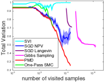
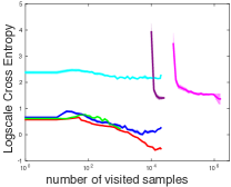
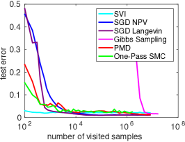
For the mixture model and logistic regression, we compare our algorithm with five general approximate Bayesian inference methods, including three sampling algorithms, i.e., one-pass sequential Monte Carlo (one-pass SMC) [3] which is an improved version of the SMC for Bayesian inference [8], stochastic gradient Langevin dynamics (SGD Langevin) [42] and Gibbs sampling, and two variational inference methods, i.e., stochastic variational inference (SVI) [19] and stochastic variant of nonparametric variational inference (SGD NPV) [15]. For sparse GP and LDA, we compare with the existing large-scale inference algorithms designed specifically for the models.

Evaluation criterion.

For the synthetic data generated by mixture model, we could calculate the true posterior, Therefore, we evaluate the performance directly through total variation and KL𝐾𝐿KL-divergence (cross entropy). For the experiments on logistic regression, sparse GP and LDA on real-world datasets, we use indirect criteria which are widely used [7, 13, 18, 34, 19] because of the intractability of the posterior. We keep the same memory budget for Monte Carlo based algorithms if their computational cost is acceptable. To demonstrate the efficiency of each algorithm in utilizing data, we use the number of data visited cumulatively as x-axis.

For the details of the model specification, experimental setups, additional results and algorithm derivations for sparse GP and LDA, please refer to the Appendix H.

Mixture Models.

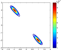
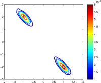
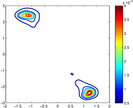
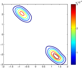
We conduct comparison on a simple yet interesting mixture model [42], the observations xip𝒩(θ1,σx2)+(1p)𝒩(θ1+θ2,σx2)similar-tosubscript𝑥𝑖𝑝𝒩subscript𝜃1superscriptsubscript𝜎𝑥21𝑝𝒩subscript𝜃1subscript𝜃2superscriptsubscript𝜎𝑥2x_{i}\sim p\mathcal{N}(\theta_{1},\sigma_{x}^{2})+(1-p)\mathcal{N}(\theta_{1}+\theta_{2},\sigma_{x}^{2}) and θ1𝒩(0,σ12)similar-tosubscript𝜃1𝒩0superscriptsubscript𝜎12\theta_{1}\sim\mathcal{N}(0,\sigma_{1}^{2}), θ2𝒩(0,σ22)similar-tosubscript𝜃2𝒩0superscriptsubscript𝜎22\theta_{2}\sim\mathcal{N}(0,\sigma_{2}^{2}), where (σ1,σ2)=(1,1)subscript𝜎1subscript𝜎211(\sigma_{1},\sigma_{2})=(1,1), σx=2.5subscript𝜎𝑥2.5\sigma_{x}=2.5 and p=0.5𝑝0.5p=0.5. The means of two Gaussians are tied together making θ1subscript𝜃1\theta_{1} and θ2subscript𝜃2\theta_{2} correlated in the posterior. We generate 100010001000 data from the model with (θ1,θ2)=(1,2)subscript𝜃1subscript𝜃212(\theta_{1},\theta_{2})=(1,-2). This is one mode of the posterior, there is another equivalent mode at (θ1,θ2)=(1,2)subscript𝜃1subscript𝜃212(\theta_{1},\theta_{2})=(-1,2).

Refer to caption Refer to caption Refer to caption Refer to caption
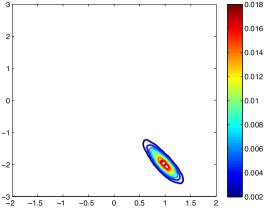
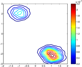
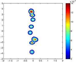
(1) True Posterior (2) Estimated Posterior (3) Total Variation (4) Cross Entropy
Figure 1: Experimental results for mixture model on synthetic dataset.
Refer to caption Refer to caption Refer to caption
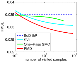
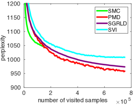
(1) Logistic regression on MNIST (2) Sparse GP on music data (3) LDA on wikipedia data
Figure 2: Experimental results on several different models for real-world datasets.

We initialize all algorithms with prior on (θ1,θ2)subscript𝜃1subscript𝜃2(\theta_{1},\theta_{2}). We repeat the experiments 101010 times and report the average results. We keep the same memory for all except SVI. The true posterior and the one generated by our method is illustrated in Figure 1 (1)(2). PMD fits both modes well and recovers nicely the posterior while other algorithms either miss a mode or fail to fit the multimodal density. For the competitors’ results, please refer to Appendix H. PMD achieves the best performance in terms of total variation and cross entropy as shown in Figure 1 (3)(4). This experiment clearly indicates our algorithm is able to take advantages of nonparametric model to capture multiple modes.

Bayesian Logistic Regression.

We test our algorithm on logistic regression with non-conjugate prior for handwritten digits classification on the MNIST8M 8 vs. 6 dataset. The dataset contains about 1.61.61.6M training samples and 193219321932 testing samples. We initialize all algorithms with same prior and terminate the stochastic algorithms after 5 passes through the dataset. We keep 100010001000 samples for Monte Carlo based algorithms, except Gibbs sampling whose computation cost is unaffordable. We repeat the experiments 101010 times and the results are reported in Figure 2(1). Obviously, Gibbs sampling [20], which needs to scan the whole dataset, is not suitable for large-scale problem. In this experiment, SVI performs best at first, which is expectable because learning in the Gaussian family is simpler comparing to nonparametric density family. Our algorithm achieves comparable performance in nonparametric form after fed with enough data, 98.8%percent98.898.8\%, to SVI which relies on carefully designed lower bound of the log-likelihood [22]. SGD NPV is flexible with mixture models family, however, its speed becomes the bottleneck. For SGD NPV, the speed is dragged down for the use of L-BFGS to optimize the second-order approximation of ELBO.

Sparse Gaussian Processes.

We use sparse GPs models to predict the year of songs [5]. In this task, we compare to the SVI for sparse GPs [19, 18]and one-pass SMC. We also included subset of data approximation (SoD) [35] as baseline. The data contains about 0.50.50.5M songs, each represented by 909090-dimension features. We terminate the stochastic algorithms after 2 passes of dataset. We use 161616 particles in both SMC and PMD. The number of inducing inputs in sparse GP is set to be 210superscript2102^{10}, and other hyperparameters of sparse GP are fixed for all methods. We run experiments 101010 times and results are reported in Figure. 2(2). Our algorithm achieves the best RMSE 0.0270.0270.027, significantly better than one-pass SMC and SVI.

Latent Dirichlet Allocation.

We compare to SVI [19], stochastic gradient Riemannian Langevin dynamic (SGRLD) [34], and SMC specially designed for LDA [6] on Wikipedia dataset [34]. The dataset contains 0.150.150.15M documents, about 222M words and 800080008000 vocabulary. Since we evaluate their performances in terms of perplexity, which is integral over posterior, we do not need to recover the posterior, and therefore, we follow the same setting in [1, 27], where one particle is used in SMC and PMD to save the cost. We set topic number to 100100100 and fix other hyperparameters to be fair to all algorithms. We stop the stochastic algorithms after 5 passes of dataset. The results are reported in Figure 2(3). The top words from several topics found by our algorithm are illustrated in Appendix H. Our algorithm achieves the best perplexity, significantly better than SGRLD and SVI. In this experiment, SMC performs well at the beginning since it treats each documents equally and updates with full likelihood. However, SMC only uses each datum once, while the stochastic algorithms, e.g., SGRLD, SVI and our PMD, could further refine the solution by running the dataset multiple times.

7 Conclusion

Our work contributes towards achieving better trade-off between efficiency, flexibility and provability in approximate Bayesian inference from optimization perspective. The proposed algorithm, Particle Mirror Descent, successfully combines stochastic mirror descent and nonparametric density approximation. Theoretically, the algorithm enjoys a rate O(1/m)𝑂1𝑚O(1/\sqrt{m}) in terms of both integral approximation and KL𝐾𝐿KL-divergence, with O(m)𝑂𝑚O(m) particles. Practically, the algorithm achieves competitive performance to existing state-of-the-art inference algorithms in mixture models, logistic regression, sparse Gaussian processes and latent Dirichlet analysis on several large-scale datasets.

Acknowledgements

We thank the anonymous referees for their valuable suggestions. This project was supported in part by NSF/NIH BIGDATA 1R01GM108341, ONR N00014-15-1-2340, NSF IIS-1218749, and NSF CAREER IIS-1350983.

References

  • Ahmed et al. [2012] A. Ahmed, M. Aly, J. Gonzalez, S. Narayanamurthy, and A. J. Smola. Scalable inference in latent variable models. In The 5th ACM International Conference on Web Search and Data Mining, 2012.
  • Ahn et al. [2012] S. Ahn, A. Korattikara, and M. Welling. Bayesian posterior sampling via stochastic gradient fisher scoring. In International Conference on Machine Learning, 2012.
  • Balakrishnan and Madigan [2006] S. Balakrishnan and D. Madigan. A one-pass sequential monte carlo method for bayesian analysis of massive datasets. Bayesian Analysis, 1(2):345–361, 06 2006.
  • Barron and Yang [1995] A. Barron and Y. Yang. Information theoretic determination of minimax rates of convergence. Annals of Statistics, 27:1564–1599, 1995.
  • Bertin-Mahieux et al. [2011] T. Bertin-Mahieux, D. P.W. Ellis, B. Whitman, and P. Lamere. The million song dataset. In International Conference on Music Information Retrieval, 2011.
  • Canini et al. [2009] K. R. Canini, L. Shi, and T. L. Griff iths. Online inference of topics with latent dirichlet allocation. In the Twelfth International Conference on Artificial Intelligence and Statistics, 2009.
  • Chen et al. [2014] T. Chen, E. B. Fox, and C. Guestrin. Stochastic Gradient Hamiltonian Monte Carlo. In International Conference on Machine Learning, 2014.
  • Chopin [2002] N. Chopin. A sequential particle filter method for static models. Biometrika, 89(3):539–551, 2002.
  • Crisan and Doucet [2002] D. Crisan and A. Doucet. A survey of convergence results on particle filtering methods for practitioners. Signal Processing, IEEE Transactions on, 50(3):736–746, 2002.
  • Del Moral et al. [2006] P. Del Moral, A. Doucet, and A. Jasra. Sequential monte carlo samplers. Journal of the Royal Statistical Society: Series B (Statistical Methodology), 68(3):411–436, 2006.
  • Delyon and Juditsky [1996] B. Delyon and A. Juditsky. On minimax wavelet estimators. Applied and Computational Harmonic Analysis, 3(3):215 – 228, 1996.
  • Devroye and Györfi [1985] L. Devroye and L. Györfi. Nonparametric Density Estimation: The L1subscript𝐿1L_{1} View. John Wiley and Sons, 1985.
  • Ding et al. [2014] N. Ding, Y. Fang, R. Babbush, C. Chen, R. D. Skeel, and H. Neven. Bayesian sampling using stochastic gradient thermostats. In Advances in Neural Information Processing Systems 27, 2014.
  • Doucet et al. [2001] A. Doucet, N. de Freitas, and N. Gordon. Sequential Monte Carlo Methods in Practice. Springer-Verlag, 2001.
  • Gershman et al. [2012] S. Gershman, M. Hoffman, and D. M. Blei. Nonparametric variational inference. In International Conference on Machine Learning, 2012.
  • Gibbs and Su [2002] A. Gibbs and F. E.Su. On choosing and bounding probability metrics. International statistical review, 70: 419–435, 2002
  • Gland and Oudjane [2004] F. L. Gland and N. Oudjane. Stability and uniform approximation of nonlinear filters using the hilbert metric and application to particle filters. The Annals of Applied Probability, 14(1):pp. 144–187, 2004.
  • Hensman et al. [2013] J. Hensman, N. Fusi, and N. D. Lawrence. Gaussian processes for big data. In the Twenty-Ninth Conference on Uncertainty in Artificial Intelligence, 2013.
  • Hoffman et al. [2013] M. D. Hoffman, D. M. Blei, C. Wang, and J. Paisley. Stochastic variational inference. Journal of Machine Learning Research, 14:1303–1347, 2013.
  • Holmes and Held [145-168] C. C. Holmes and L. Held. Bayesian auxiliary variable models for binary and multinomial regression. Bayesian Analysis, 1(1), 2006 145-168.
  • Ihler and McAllester [2009] A. Ihler and D. McAllester. Particle belief propagation. In the Twelfth International Conference on Artificial Intelligence and Statistics, 2009.
  • Jaakkola and Jordan [1997] T. Jaakkola and M. I. Jordan. A variational approach to bayesian logistic regression models and their extensions. In Sixth International Workshop on Artificial Intelligence and Statistics, 1997.
  • Jaakkola and Jordon [1999] T. S. Jaakkola and M. I. Jordon. Learning in graphical models. chapter Improving the Mean Field Approximation via the Use of Mixture Distributions, pages 163–173. MIT Press, Cambridge, MA, USA, 1999.
  • Jordan et al. [1998] M. I. Jordan, Z. Gharamani, T. S. Jaakkola, and L. K. Saul. An introduction to variational methods for graphical models. In M. I. Jordan, editor, Learning in Graphical Models, pages 105–162. Kluwer Academic, 1998.
  • Lienart et al. [2015] T. Lienart, Y. W. Teh, and A. Doucet. Expectation particle belief propagation. In Advances in Neural Information Processing Systems, 2015.
  • Maclaurin and Adams [2014] D. Maclaurin and R. P. Adams. Firefly monte carlo: Exact MCMC with subsets of data. In the Thirtieth Conference on Uncertainty in Artificial Intelligence, 2014.
  • Mimno et al. [2012] D. Mimno, M. Hoffman, and D. Blei. Sparse stochastic inference for latent dirichlet allocation. In International Conference on Machine Learning, 2012.
  • Minka [2001] T. Minka. Expectation Propagation for approximative Bayesian inference. PhD thesis, MIT Media Labs, Cambridge, USA, 2001.
  • Minka [2005] T. Minka. Divergence measures and message passing. Report 173, Microsoft Research, 2005.
  • Neal [2001] R. M. Neal. Defining priors for distributions using dirichlet diffusion trees. Technical report, University of Toronto, 2001.
  • Neal [1993] R. M. Neal. Probabilistic inference using Markov chain Monte Carlo methods. Technical report, University of Toronto, 1993.
  • Nemirovski et al. [2009] A. Nemirovski, A. Juditsky, G. Lan, and A. Shapiro. Robust stochastic approximation approach to stochastic programming. SIAM J. on Optimization, 19(4):1574–1609, January 2009.
  • Paisley et al. [2012] J. W. Paisley, D. M. Blei, and M. I. Jordan. Variational bayesian inference with stochastic search. In International Conference on Machine Learning, 2012.
  • Patterson and Teh [2013] S. Patterson and Y. W. Teh. Stochastic gradient Riemannian Langevin dynamics on the probability simplex. In Advances in Neural Information Processing Systems, 2013.
  • Quiñonero-Candela and Rasmussen [2005] J. Quiñonero-Candela and C. E. Rasmussen. A unifying view of sparse approximate gaussian process regression. Journal of Machine Learning Research, 6:1939–1959, 2005.
  • Vollmer et al [2015] S. J. Vollmer, K. C. Zygalakis and Y. W. Teh. (non-) asymptotic properties of stochastic gradient langevin dynamics. submitted, 2015.
  • Song et al. [2011] L. Song, A. Gretton, D. Bickson, Y. Low, and C. Guestrin. Kernel belief propagation. In the Fourteenth Conference on Artificial Intelligence and Statistics, 2011.
  • Sudderth et al. [2003] E. Sudderth, A. Ihler, W. Freeman, and A. Willsky. Nonparametric belief propagation. In IEEE Conference on Computer Vision and Pattern Recognition, 2003.
  • Teh et al. [2014] Y. W. Teh, A. H. Thiéry, and S. J. Vollmer. Consistency and fluctuations for stochastic gradient Langevin dynamics. submitted, 2014.
  • Wainwright and Jordan [2008] M. J. Wainwright and M. I. Jordan. Graphical models, exponential families, and variational inference. Foundations and Trends in Machine Learning, 1(1 – 2):1–305, 2008.
  • Wand and Jones [1995] M. P. Wand and M. C. Jones. Kernel Smoothing. Chapman and Hall, London, 1995.
  • Welling and Teh [2011] M. Welling and Y.W. Teh. Bayesian learning via stochastic gradient langevin dynamics. In International Conference on Machine Learning, 2011.
  • Williams [1980] P. M. Williams. Bayesian conditionalisation and the principle of minimum information. British Journal for the Philosophy of Science, 31(2):131–144, 1980.
  • Zellner [1988] A. Zellner. Optimal Information Processing and Bayes’s Theorem. The American Statistician, 42(4), November 1988.
  • Zhu et al. [2014] J. Zhu, N. Chen, and E. P. Xing. Bayesian inference with posterior regularization and applications to infinite latent svms. Journal of Machine Learning Research, 15(1):1799–1847, January 2014.

Appendix

Appendix A Strong convexity

As we discussed, the posterior from Bayes’s rule could be viewed as the optimal of an optimization problem in Eq (1). We will show that the objective function is strongly convex w.r.t KL𝐾𝐿KL-divergence.

Proof for Lemma 1. The lemma directly results from the generalized Pythagaras theorem for Bregman divergence. Particularly, for KL𝐾𝐿KL-divergence, we have

KL(q1||q)\displaystyle KL(q_{1}||q) =\displaystyle= KL(q1||q2)+KL(q2||q)q1q2,ϕ(q)ϕ(q2)2\displaystyle KL(q_{1}||q_{2})+KL(q_{2}||q)-\langle q_{1}-q_{2},\nabla\phi(q)-\nabla\phi(q_{2})\rangle_{2}

where ϕ(q)italic-ϕ𝑞\phi(q) is the entropy of q𝑞q.

Notice that L(q)=KL(q||q)logZL(q)=KL(q||q^{*})-\log Z, where q=p(θ)ΠiNp(xi|θ)Z,Z=p(θ)ΠiNp(xi|θ)formulae-sequencesuperscript𝑞𝑝𝜃superscriptsubscriptΠ𝑖𝑁𝑝conditionalsubscript𝑥𝑖𝜃𝑍𝑍𝑝𝜃superscriptsubscriptΠ𝑖𝑁𝑝conditionalsubscript𝑥𝑖𝜃q^{*}=\frac{p(\theta)\Pi_{i}^{N}p(x_{i}|\theta)}{Z},\quad Z=\int p(\theta)\Pi_{i}^{N}p(x_{i}|\theta), we have

KL(q1||q)KL(q2||q)q1q2,ϕ(q2)ϕ(q)2=KL(q1||q2)\displaystyle KL(q_{1}||q^{*})-KL(q_{2}||q^{*})-\langle q_{1}-q_{2},\nabla\phi(q_{2})-\nabla\phi(q^{*})\rangle_{2}=KL(q_{1}||q_{2})
\displaystyle\Rightarrow KL(q1||q)KL(q2||q)q1q2,logq2logq2=KL(q1||q2)\displaystyle KL(q_{1}||q^{*})-KL(q_{2}||q^{*})-\langle q_{1}-q_{2},\log q_{2}-\log q^{*}\rangle_{2}=KL(q_{1}||q_{2})
\displaystyle\Rightarrow KL(q1||q)KL(q2||q)q1q2,logq2log(p(θ)ΠiNp(xi|θ))2+q1q2,logZ20=KL(q1||q2)\displaystyle KL(q_{1}||q^{*})-KL(q_{2}||q^{*})-\langle q_{1}-q_{2},\log q_{2}-\log\big{(}p(\theta)\Pi_{i}^{N}p(x_{i}|\theta)\big{)}\rangle_{2}+\underbrace{\langle q_{1}-q_{2},\log Z\rangle_{2}}_{0}=KL(q_{1}||q_{2})
\displaystyle\Rightarrow L(q1)L(q2)q1q2,L(q2)2=KL(q1||q2)\displaystyle L(q_{1})-L(q_{2})-\langle q_{1}-q_{2},\nabla L(q_{2})\rangle_{2}=KL(q_{1}||q_{2})

\blacksquare

Appendix B Finite Convergence of Stochastic Mirror Descent with Inexact Prox-Mapping in Density Space

Since the prox-mapping of stochastic mirror descent is intractable when directly being applied to the optimization problem (1), we propose the ϵitalic-ϵ\epsilon-inexact prox-mapping within the stochastic mirror descent framework in Section 3. Instead of solving the prox-mapping exactly, we approximate the solution with ϵitalic-ϵ\epsilon error. In this section, we will show as long as the approximation error is tolerate, the stochastic mirror descent algorithm still converges.

Theorem 2 Denote q=argminq𝒫L(q)superscript𝑞subscriptargmin𝑞𝒫𝐿𝑞q^{*}=\mathop{\mathrm{argmin}}_{q\in\mathcal{P}}L(q), the stochastic mirror descent with inexact prox-mapping after T𝑇T steps gives

  1. (a)

    the recurrence: tTfor-all𝑡𝑇\forall t\leqslant T, 𝔼[KL(q||q~t+1)]ϵt+(1γt)𝔼[KL(q||q~t)]+γt2𝔼gt22\mathbb{E}[KL(q^{*}||\tilde{q}_{t+1})]\leqslant\epsilon_{t}+(1-\gamma_{t})\mathbb{E}[KL(q^{*}||\tilde{q}_{t})]+\frac{\gamma_{t}^{2}\mathbb{E}\|g_{t}\|^{2}_{\infty}}{2}

  2. (b)

    the sub-optimality: 𝔼[KL(q¯T||q)]𝔼[L(q¯T)L(q)]212t=1Tγt2+t=1Tϵt+D1t=1Tγt\mathbb{E}[KL(\bar{q}_{T}||q^{*})]\leqslant\mathbb{E}[L(\bar{q}_{T})-L(q^{*})]\leqslant\frac{\mathcal{M}^{2}\cdot\frac{1}{2}\sum_{t=1}^{T}\gamma_{t}^{2}+\sum_{t=1}^{T}\epsilon_{t}+D_{1}}{\sum_{t=1}^{T}\gamma_{t}} where q¯T=t=1Tγtq~t/t=1Tγtsubscript¯𝑞𝑇superscriptsubscript𝑡1𝑇subscript𝛾𝑡subscript~𝑞𝑡superscriptsubscript𝑡1𝑇subscript𝛾𝑡\bar{q}_{T}=\sum_{t=1}^{T}\gamma_{t}\tilde{q}_{t}/\sum_{t=1}^{T}\gamma_{t} and D1=KL(q||q~1)D_{1}=KL(q^{*}||\tilde{q}_{1}) and 2:=max1tT𝔼gt2assignsuperscript2subscript1𝑡𝑇𝔼superscriptsubscriptnormsubscript𝑔𝑡2\mathcal{M}^{2}:=\max_{1\leqslant t\leqslant T}\mathbb{E}\|g_{t}\|_{\infty}^{2}.

Remark. Based on [32], one can immediately see that, to guarantee the usual rate of convergence, the error ϵtsubscriptitalic-ϵ𝑡\epsilon_{t} can be of order O(γt2)𝑂superscriptsubscript𝛾𝑡2O(\gamma_{t}^{2}). The first recurrence implies an overall O(1/T)𝑂1𝑇O(1/T) rate of convergence for the KL𝐾𝐿KL-divergence when the stepsize γtsubscript𝛾𝑡\gamma_{t} is as small as O(1/t)𝑂1𝑡O(1/t) and error ϵtsubscriptitalic-ϵ𝑡\epsilon_{t} is as small as O(1/t2)𝑂1superscript𝑡2O(1/t^{2}). The second result implies an overall O(1/T)𝑂1𝑇O(1/\sqrt{T}) rate of convergence for objective function when larger stepsize γt=O(1/T)subscript𝛾𝑡𝑂1𝑇\gamma_{t}=O(1/\sqrt{T}) and larger error ϵt=O(1/t)subscriptitalic-ϵ𝑡𝑂1𝑡\epsilon_{t}=O(1/t) are adopted.

Proof for Theorem 2. (a) By first-order optimality condition, q~t+1Pq~tϵt(γtgt)subscript~𝑞𝑡1superscriptsubscript𝑃subscript~𝑞𝑡subscriptitalic-ϵ𝑡subscript𝛾𝑡subscript𝑔𝑡\tilde{q}_{t+1}\in P_{\tilde{q}_{t}}^{\epsilon_{t}}(\gamma_{t}g_{t}) is equivalent as

γtgt+log(q~t+1)log(q~t),q~t+1qL2ϵt,q𝒫,formulae-sequencesubscriptsubscript𝛾𝑡subscript𝑔𝑡subscript~𝑞𝑡1subscript~𝑞𝑡subscript~𝑞𝑡1𝑞subscript𝐿2subscriptitalic-ϵ𝑡for-all𝑞𝒫\langle\gamma_{t}g_{t}+\log(\tilde{q}_{t+1})-\log(\tilde{q}_{t}),\tilde{q}_{t+1}-q\rangle_{L_{2}}\leqslant\epsilon_{t},\forall q\in\mathcal{P},

which implies that

γtgt,q~t+1q2log(q~t)log(q~t+1),q~t+1q2+ϵt=KL(q||q~t)KL(q||q~t+1)KL(q~t+1||q~t)+ϵt\displaystyle\langle\gamma_{t}g_{t},\tilde{q}_{t+1}-q\rangle_{2}\leqslant\langle\log(\tilde{q}_{t})-\log(\tilde{q}_{t+1}),\tilde{q}_{t+1}-q\rangle_{2}+\epsilon_{t}=KL(q||\tilde{q}_{t})-KL(q||\tilde{q}_{t+1})-KL(\tilde{q}_{t+1}||\tilde{q}_{t})+\epsilon_{t}

Hence,

γtgt,q~tq2KL(q||q~t)KL(q||q~t+1)KL(q~t+1||q~t)+γtgt,q~tq~t+12+ϵt.\displaystyle\langle\gamma_{t}g_{t},\tilde{q}_{t}-q\rangle_{2}\leqslant KL(q||\tilde{q}_{t})-KL(q||\tilde{q}_{t+1})-KL(\tilde{q}_{t+1}||\tilde{q}_{t})+\langle\gamma_{t}g_{t},\tilde{q}_{t}-\tilde{q}_{t+1}\rangle_{2}+\epsilon_{t}. (8)

By Young’s inequality, we have

γtgt,q~tq~t+1212q~tq~t+112+γt22gt2.subscriptsubscript𝛾𝑡subscript𝑔𝑡subscript~𝑞𝑡subscript~𝑞𝑡1212superscriptsubscriptnormsubscript~𝑞𝑡subscript~𝑞𝑡112superscriptsubscript𝛾𝑡22superscriptsubscriptnormsubscript𝑔𝑡2\displaystyle\langle\gamma_{t}g_{t},\tilde{q}_{t}-\tilde{q}_{t+1}\rangle_{2}\leqslant\frac{1}{2}\|\tilde{q}_{t}-\tilde{q}_{t+1}\|_{1}^{2}+\frac{\gamma_{t}^{2}}{2}\|g_{t}\|_{\infty}^{2}. (9)

Also, from Pinsker’s inequality, we have

KL(q~t+1||q~t)12q~tq~t+112.\displaystyle KL(\tilde{q}_{t+1}||\tilde{q}_{t})\geqslant\frac{1}{2}\|\tilde{q}_{t}-\tilde{q}_{t+1}\|_{1}^{2}. (10)

Therefore, combining (8), (9), and (10), we have q𝒫for-all𝑞𝒫\forall q\in\mathcal{P}

γtgt,q~tq2ϵt+KL(q||q~t)KL(q||q~t+1)+γt22gt2\displaystyle\langle\gamma_{t}g_{t},\tilde{q}_{t}-q\rangle_{2}\leqslant\epsilon_{t}+{KL(q||\tilde{q}_{t})}-{KL(q||\tilde{q}_{t+1})}+\frac{\gamma_{t}^{2}}{2}\|g_{t}\|_{\infty}^{2}

Plugging qsuperscript𝑞q^{*} and taking expectation on both sides, the LHS becomes

𝔼x[q~tq,γtgt]subscript𝔼𝑥delimited-[]subscript~𝑞𝑡superscript𝑞subscript𝛾𝑡subscript𝑔𝑡\displaystyle\mathbb{E}_{x}\bigg{[}\langle\tilde{q}_{t}-q^{*},\gamma_{t}g_{t}\rangle\bigg{]} =\displaystyle= 𝔼x[q~tq,γt𝔼[gt]|x[t1]]=𝔼x[q~tq,γtL(q~t)],subscript𝔼𝑥delimited-[]conditionalsubscript~𝑞𝑡superscript𝑞subscript𝛾𝑡𝔼delimited-[]subscript𝑔𝑡subscript𝑥delimited-[]𝑡1subscript𝔼𝑥delimited-[]subscript~𝑞𝑡superscript𝑞subscript𝛾𝑡𝐿subscript~𝑞𝑡\displaystyle\mathbb{E}_{x}\bigg{[}\langle\tilde{q}_{t}-q^{*},\gamma_{t}\mathbb{E}[g_{t}]\rangle\bigg{|}x_{[t-1]}\bigg{]}=\mathbb{E}_{x}\bigg{[}\langle\tilde{q}_{t}-q^{*},\gamma_{t}\nabla L(\tilde{q}_{t})\rangle\bigg{]},

Therefore, we have

𝔼x[q~tq,γtL(q~t)]ϵt+𝔼x[KL(q||q~t)]𝔼x[KL(q||q~t+1)]+γt22𝔼xgt2\displaystyle\mathbb{E}_{x}\bigg{[}\langle\tilde{q}_{t}-q^{*},\gamma_{t}\nabla L(\tilde{q}_{t})\rangle\bigg{]}\leqslant\epsilon_{t}+\mathbb{E}_{x}\big{[}{KL(q^{*}||\tilde{q}_{t})}\big{]}-\mathbb{E}_{x}\big{[}{KL(q^{*}||\tilde{q}_{t+1})}\big{]}+\frac{\gamma_{t}^{2}}{2}\mathbb{E}_{x}\|g_{t}\|_{\infty}^{2} (11)

Because the objective function is 111-strongly convex w.r.t. KL𝐾𝐿KL-divergence,

qq,L(q)L(q)=KL(q||q)+KL(q||q),\displaystyle\langle q^{\prime}-q,\nabla L(q^{\prime})-\nabla L(q)\rangle=KL(q^{\prime}||q)+KL(q||q^{\prime}),

and the optimality condition, we have

q~tq,L(q~t)KL(q||q~t)\displaystyle\langle\tilde{q}_{t}-q^{*},\nabla L(\tilde{q}_{t})\rangle\geqslant KL(q^{*}||\tilde{q}_{t})

we obtain the recursion with inexact prox-mapping,

𝔼x[KL(q||q~t+1)]ϵt+(1γt)𝔼x[KL(q||q~t)]+γt222\displaystyle\mathbb{E}_{x}[KL(q^{*}||\tilde{q}_{t+1})]\leqslant\epsilon_{t}+(1-\gamma_{t})\mathbb{E}_{x}[KL(q^{*}||\tilde{q}_{t})]+\frac{\gamma_{t}^{2}}{2}\mathcal{M}^{2}

(b) Summing over t=1,,T𝑡1𝑇t=1,\ldots,T of equation (11), we get

t=1T𝔼x[q~tq,γtL(q~t)]t=1Tϵt+KL(q||q~1)+t=1Tγt222\displaystyle\sum_{t=1}^{T}\mathbb{E}_{x}[\langle\tilde{q}_{t}-q^{*},\gamma_{t}\nabla L(\tilde{q}_{t})\rangle]\leqslant\sum_{t=1}^{T}\epsilon_{t}+{KL(q^{*}||\tilde{q}_{1})}+\sum_{t=1}^{T}\frac{\gamma_{t}^{2}}{2}\mathcal{M}^{2}

By convexity and optimality condition, this leads to

(t=1Tγt)𝔼x[L(q¯T)L(q)]𝔼x[t=1Tγt(L(q~t)L(q))]t=1Tϵt+KL(q||q~1)+t=1Tγt222\displaystyle\left(\sum_{t=1}^{T}\gamma_{t}\right)\mathbb{E}_{x}[L(\bar{q}_{T})-L(q^{*})]\leqslant\mathbb{E}_{x}\left[\sum_{t=1}^{T}\gamma_{t}(L(\tilde{q}_{t})-L(q^{*}))\right]\leqslant\sum_{t=1}^{T}\epsilon_{t}+{KL(q^{*}||\tilde{q}_{1})}+\sum_{t=1}^{T}\frac{\gamma_{t}^{2}}{2}\mathcal{M}^{2}

Furthermore, combined with the 111-strongly-convexity, it immediately follows that

𝔼x[KL(q¯T||q)]\displaystyle\mathbb{E}_{x}[KL(\bar{q}_{T}||q^{*})] \displaystyle\leqslant 𝔼x[L(q¯T)L(q)]12t=1Tγt22+t=1Tϵt+D1t=1Tγt.subscript𝔼𝑥delimited-[]𝐿subscript¯𝑞𝑇𝐿superscript𝑞12superscriptsubscript𝑡1𝑇superscriptsubscript𝛾𝑡2superscript2superscriptsubscript𝑡1𝑇subscriptitalic-ϵ𝑡subscript𝐷1superscriptsubscript𝑡1𝑇subscript𝛾𝑡\displaystyle\mathbb{E}_{x}[L(\bar{q}_{T})-L(q^{*})]\leqslant\frac{\frac{1}{2}\sum_{t=1}^{T}\gamma_{t}^{2}\mathcal{M}^{2}+\sum_{t=1}^{T}\epsilon_{t}+D_{1}}{\sum_{t=1}^{T}\gamma_{t}}.

\blacksquare

Appendix C Convergence Analysis for Integral Approximation

In this section, we provide the details of the convergence analysis of the proposed algorithm in terms of integral approximation w.r.t. the true posterior using a good initialization.

Assume that the prior p(θ)𝑝𝜃p(\theta) has support ΩΩ\Omega cover true posterior distribution q(θ)superscript𝑞𝜃q^{*}(\theta), then, we could represent

q(θ)={q(θ)=α(θ)p(θ),α(θ)p(θ)𝑑θ=1,0α(θ)C}.superscript𝑞𝜃formulae-sequence𝑞𝜃𝛼𝜃𝑝𝜃formulae-sequence𝛼𝜃𝑝𝜃differential-d𝜃10𝛼𝜃𝐶q^{*}(\theta)\in\mathcal{F}=\bigg{\{}q(\theta)=\alpha(\theta)p(\theta),\int\alpha(\theta)p(\theta)d\theta=1,0\leqslant\alpha(\theta)\leqslant C\bigg{\}}.

Therefore, one can show

Lemma 7

qfor-all𝑞\forall q\in\mathcal{F}, let {θi}i=1msuperscriptsubscriptsubscript𝜃𝑖𝑖1𝑚\{\theta_{i}\}_{i=1}^{m} is i.i.d.  sampled from p(θ)𝑝𝜃p(\theta), we could construct q^(θ)=i=1mα(θi)δ(θi)imα(θi)^𝑞𝜃superscriptsubscript𝑖1𝑚𝛼subscript𝜃𝑖𝛿subscript𝜃𝑖superscriptsubscript𝑖𝑚𝛼subscript𝜃𝑖\hat{q}(\theta)=\sum_{i=1}^{m}\frac{\alpha(\theta_{i})\delta(\theta_{i})}{\sum_{i}^{m}\alpha(\theta_{i})}, such that f(θ):d:for-all𝑓𝜃superscript𝑑\forall f(\theta):\mathbb{R}^{d}\rightarrow\mathbb{R} bounded and integrable,

𝔼[|q^(θ)f(θ)𝑑θq(θ)f(θ)𝑑θ|]2Cfm.𝔼delimited-[]^𝑞𝜃𝑓𝜃differential-d𝜃𝑞𝜃𝑓𝜃differential-d𝜃2𝐶subscriptnorm𝑓𝑚\mathbb{E}{\bigg{[}\bigg{|}\int\hat{q}(\theta)f(\theta)d\theta-\int q(\theta)f(\theta)d\theta\bigg{|}\bigg{]}}\leqslant\frac{2\sqrt{C}\|f\|_{\infty}}{\sqrt{m}}.

Proof 

Given q(θ)𝑞𝜃q(\theta), we sample i.i.d.{θi}i=1msuperscriptsubscriptsubscript𝜃𝑖𝑖1𝑚\{\theta_{i}\}_{i=1}^{m} from p(θ)𝑝𝜃p(\theta), and construct a function

q^(θ)=1mi=1mα(θi)δ(θi,θ).^𝑞𝜃1𝑚superscriptsubscript𝑖1𝑚𝛼subscript𝜃𝑖𝛿subscript𝜃𝑖𝜃\displaystyle\hat{q}(\theta)=\frac{1}{m}\sum_{i=1}^{m}\alpha(\theta_{i})\delta(\theta_{i},\theta).

It is obviously that

𝔼θ[q^(θ)]=𝔼θ[1mi=1mα(θi)δ(θi,θ)]=1mi=1m𝔼θ[α(θi)δ(θi,θ)]=q(θ)subscript𝔼𝜃delimited-[]^𝑞𝜃subscript𝔼𝜃delimited-[]1𝑚superscriptsubscript𝑖1𝑚𝛼subscript𝜃𝑖𝛿subscript𝜃𝑖𝜃1𝑚superscriptsubscript𝑖1𝑚subscript𝔼𝜃delimited-[]𝛼subscript𝜃𝑖𝛿subscript𝜃𝑖𝜃𝑞𝜃\displaystyle\mathbb{E}_{\theta}[\hat{q}(\theta)]=\mathbb{E}_{\theta}\bigg{[}\frac{1}{m}\sum_{i=1}^{m}\alpha(\theta_{i})\delta(\theta_{i},\theta)\bigg{]}=\frac{1}{m}\sum_{i=1}^{m}\mathbb{E}_{\theta}\bigg{[}\alpha(\theta_{i})\delta(\theta_{i},\theta)\bigg{]}=q(\theta)

and

𝔼θ[q^(θ)f(θ)𝑑θ]=𝔼θ[1mi=1mα(θi)f(θi)]=1mi=1m𝔼θ[α(θi)f(θi)]=q(θ)f(θ)𝑑θsubscript𝔼𝜃delimited-[]^𝑞𝜃𝑓𝜃differential-d𝜃subscript𝔼𝜃delimited-[]1𝑚superscriptsubscript𝑖1𝑚𝛼subscript𝜃𝑖𝑓subscript𝜃𝑖1𝑚superscriptsubscript𝑖1𝑚subscript𝔼𝜃delimited-[]𝛼subscript𝜃𝑖𝑓subscript𝜃𝑖𝑞𝜃𝑓𝜃differential-d𝜃\displaystyle\mathbb{E}_{\theta}\bigg{[}\int\hat{q}(\theta)f(\theta)d\theta\bigg{]}=\mathbb{E}_{\theta}\bigg{[}\frac{1}{m}\sum_{i=1}^{m}\alpha(\theta_{i})f(\theta_{i})\bigg{]}=\frac{1}{m}\sum_{i=1}^{m}\mathbb{E}_{\theta}\bigg{[}\alpha(\theta_{i})f(\theta_{i})\bigg{]}=\int q(\theta)f(\theta)d\theta

Then,

𝔼θ[|q^(θ)f(θ)𝑑θq(θ)f(θ)𝑑θ|2]=𝔼θ[|q^(θ)f(θ)𝑑θ𝔼θ[q^(θ)f(θ)𝑑θ]|2]subscript𝔼𝜃delimited-[]superscript^𝑞𝜃𝑓𝜃differential-d𝜃𝑞𝜃𝑓𝜃differential-d𝜃2subscript𝔼𝜃delimited-[]superscript^𝑞𝜃𝑓𝜃differential-d𝜃subscript𝔼𝜃delimited-[]^𝑞𝜃𝑓𝜃differential-d𝜃2\displaystyle\mathbb{E}_{\theta}\bigg{[}\bigg{|}\int\hat{q}(\theta)f(\theta)d\theta-\int q(\theta)f(\theta)d\theta\bigg{|}^{2}\bigg{]}=\mathbb{E}_{\theta}\bigg{[}\bigg{|}\int\hat{q}(\theta)f(\theta)d\theta-\mathbb{E}_{\theta}\bigg{[}\int\hat{q}(\theta)f(\theta)d\theta\bigg{]}\bigg{|}^{2}\bigg{]}
=1m(𝔼θα(θi)f(θi)22𝔼θ[α(θi)f(θi)]22)1m𝔼θα(θi)f(θi)22=1mα(θ)2f(θ)2π(θ)𝑑θabsent1𝑚subscript𝔼𝜃superscriptsubscriptnorm𝛼subscript𝜃𝑖𝑓subscript𝜃𝑖22superscriptsubscriptnormsubscript𝔼𝜃delimited-[]𝛼subscript𝜃𝑖𝑓subscript𝜃𝑖221𝑚subscript𝔼𝜃superscriptsubscriptnorm𝛼subscript𝜃𝑖𝑓subscript𝜃𝑖221𝑚𝛼superscript𝜃2𝑓superscript𝜃2𝜋𝜃differential-d𝜃\displaystyle=\frac{1}{m}\bigg{(}\mathbb{E}_{\theta}\|\alpha(\theta_{i})f(\theta_{i})\|_{2}^{2}-\|\mathbb{E}_{\theta}[\alpha(\theta_{i})f(\theta_{i})]\|_{2}^{2}\bigg{)}\leqslant\frac{1}{m}\mathbb{E}_{\theta}\|\alpha(\theta_{i})f(\theta_{i})\|_{2}^{2}=\frac{1}{m}\int\alpha(\theta)^{2}f(\theta)^{2}\pi(\theta)d\theta
=1mα(θ)f(θ)2q(θ)𝑑θCmf(θ)2α(θ)q(θ)𝑑θCmf(θ)2α(θ)absent1𝑚𝛼𝜃𝑓superscript𝜃2𝑞𝜃differential-d𝜃𝐶𝑚superscriptsubscriptnorm𝑓𝜃2𝛼𝜃𝑞𝜃differential-d𝜃𝐶𝑚superscriptsubscriptnorm𝑓𝜃2subscriptnorm𝛼𝜃\displaystyle=\frac{1}{m}\int\alpha(\theta)f(\theta)^{2}q(\theta)d\theta\leqslant\frac{{C}}{m}\|f(\theta)\|_{\infty}^{2}\int\alpha(\theta)q(\theta)d\theta\leqslant\frac{{C}}{m}\|f(\theta)\|_{\infty}^{2}\|\alpha(\theta)\|_{\infty}

By Jensen’s inequality, we have

𝔼θ[|q^(θ)f(θ)𝑑θq(θ)f(θ)𝑑θ|]𝔼θ[|q^(θ)f(θ)𝑑θq(θ)f(θ)𝑑θ|2]Cf(θ)msubscript𝔼𝜃delimited-[]^𝑞𝜃𝑓𝜃differential-d𝜃𝑞𝜃𝑓𝜃differential-d𝜃subscript𝔼𝜃delimited-[]superscript^𝑞𝜃𝑓𝜃differential-d𝜃𝑞𝜃𝑓𝜃differential-d𝜃2𝐶subscriptnorm𝑓𝜃𝑚\displaystyle\mathbb{E}_{\theta}\bigg{[}\bigg{|}\int\hat{q}(\theta)f(\theta)d\theta-\int q(\theta)f(\theta)d\theta\bigg{|}\bigg{]}\leqslant\sqrt{\mathbb{E}_{\theta}\bigg{[}\bigg{|}\int\hat{q}(\theta)f(\theta)d\theta-\int q(\theta)f(\theta)d\theta\bigg{|}^{2}\bigg{]}}\leqslant\frac{\sqrt{C}\|f(\theta)\|_{\infty}}{\sqrt{m}}

Apply the above conclusion to f(θ)=1𝑓𝜃1f(\theta)=1, we have

𝔼[|1mimαi1|]Cm𝔼delimited-[]1𝑚superscriptsubscript𝑖𝑚subscript𝛼𝑖1𝐶𝑚\displaystyle\mathbb{E}\bigg{[}\bigg{|}\frac{1}{m}\sum_{i}^{m}\alpha_{i}-1\bigg{|}\bigg{]}\leqslant\frac{\sqrt{C}}{\sqrt{m}}

Let q~(θ)=imα(θi)δ(θi,)imα(θi)~𝑞𝜃superscriptsubscript𝑖𝑚𝛼subscript𝜃𝑖𝛿subscript𝜃𝑖superscriptsubscript𝑖𝑚𝛼subscript𝜃𝑖\tilde{q}(\theta)=\frac{\sum_{i}^{m}\alpha(\theta_{i})\delta(\theta_{i},\cdot)}{\sum_{i}^{m}\alpha(\theta_{i})}, then imαiimαi=1superscriptsubscript𝑖𝑚subscript𝛼𝑖superscriptsubscript𝑖𝑚subscript𝛼𝑖1\sum_{i}^{m}\frac{\alpha_{i}}{\sum_{i}^{m}\alpha_{i}}=1, and

𝔼θ[|q~(θ)f(θ)𝑑θq^(θ)f(θ)𝑑θ|]=𝔼θ[|1imα(θi)imα(θi)f(θi)1mimα(θi)f(θi)|]subscript𝔼𝜃delimited-[]~𝑞𝜃𝑓𝜃differential-d𝜃^𝑞𝜃𝑓𝜃differential-d𝜃subscript𝔼𝜃delimited-[]1superscriptsubscript𝑖𝑚𝛼subscript𝜃𝑖superscriptsubscript𝑖𝑚𝛼subscript𝜃𝑖𝑓subscript𝜃𝑖1𝑚superscriptsubscript𝑖𝑚𝛼subscript𝜃𝑖𝑓subscript𝜃𝑖\displaystyle\mathbb{E}_{\theta}\bigg{[}\bigg{|}\int\tilde{q}(\theta)f(\theta)d\theta-\int\hat{q}(\theta)f(\theta)d\theta\bigg{|}\bigg{]}=\mathbb{E}_{\theta}\bigg{[}\bigg{|}\frac{1}{\sum_{i}^{m}\alpha(\theta_{i})}\sum_{i}^{m}\alpha(\theta_{i})f(\theta_{i})-\frac{1}{m}\sum_{i}^{m}\alpha(\theta_{i})f(\theta_{i})\bigg{|}\bigg{]}
=\displaystyle= 𝔼θ[|1imα(θi)m|1imα(θi)imα(θi)f(θi)]subscript𝔼𝜃delimited-[]1superscriptsubscript𝑖𝑚𝛼subscript𝜃𝑖𝑚norm1superscriptsubscript𝑖𝑚𝛼subscript𝜃𝑖superscriptsubscript𝑖𝑚𝛼subscript𝜃𝑖𝑓subscript𝜃𝑖\displaystyle\mathbb{E}_{\theta}\bigg{[}\bigg{|}1-\frac{\sum_{i}^{m}\alpha(\theta_{i})}{m}\bigg{|}\bigg{\|}\frac{1}{\sum_{i}^{m}\alpha(\theta_{i})}\sum_{i}^{m}\alpha(\theta_{i})f(\theta_{i})\bigg{\|}\bigg{]}
=\displaystyle= 𝔼θ[|1imα(θi)m|1imα(θi)imα(θi)|f(θi)|]𝔼[|1imαimf(θ)|]Cf(θ)msubscript𝔼𝜃delimited-[]1superscriptsubscript𝑖𝑚𝛼subscript𝜃𝑖𝑚1superscriptsubscript𝑖𝑚𝛼subscript𝜃𝑖superscriptsubscript𝑖𝑚𝛼subscript𝜃𝑖𝑓subscript𝜃𝑖𝔼delimited-[]1superscriptsubscript𝑖𝑚subscript𝛼𝑖𝑚subscriptnorm𝑓𝜃𝐶subscriptnorm𝑓𝜃𝑚\displaystyle\mathbb{E}_{\theta}\bigg{[}\bigg{|}1-\frac{\sum_{i}^{m}\alpha(\theta_{i})}{m}\bigg{|}\frac{1}{\sum_{i}^{m}\alpha(\theta_{i})}\sum_{i}^{m}\alpha(\theta_{i})|f(\theta_{i})|\bigg{]}\leqslant\mathbb{E}\bigg{[}\bigg{|}1-\frac{\sum_{i}^{m}\alpha_{i}}{m}\|f(\theta)\|_{\infty}\bigg{|}\bigg{]}\leqslant\frac{\sqrt{C}\|f(\theta)\|_{\infty}}{\sqrt{m}}

Then, we have achieve our conclusion that

𝔼θ[|q~(θ)f(θ)𝑑θq(θ)f(θ)𝑑θ|]subscript𝔼𝜃delimited-[]~𝑞𝜃𝑓𝜃differential-d𝜃𝑞𝜃𝑓𝜃differential-d𝜃\displaystyle\mathbb{E}_{\theta}\bigg{[}\bigg{|}\int\tilde{q}(\theta)f(\theta)d\theta-\int q(\theta)f(\theta)d\theta\bigg{|}\bigg{]}
\displaystyle\leqslant 𝔼θ[|q^(θ)f(θ)𝑑θq(θ)f(θ)𝑑θ|]+𝔼θ[|q~(θ)f(θ)𝑑θq^(θ)f(θ)𝑑θ|]subscript𝔼𝜃delimited-[]^𝑞𝜃𝑓𝜃differential-d𝜃𝑞𝜃𝑓𝜃differential-d𝜃subscript𝔼𝜃delimited-[]~𝑞𝜃𝑓𝜃differential-d𝜃^𝑞𝜃𝑓𝜃differential-d𝜃\displaystyle\mathbb{E}_{\theta}\bigg{[}\bigg{|}\int\hat{q}(\theta)f(\theta)d\theta-\int q(\theta)f(\theta)d\theta\bigg{|}\bigg{]}+\mathbb{E}_{\theta}\bigg{[}\bigg{|}\int\tilde{q}(\theta)f(\theta)d\theta-\int\hat{q}(\theta)f(\theta)d\theta\bigg{|}\bigg{]}
\displaystyle\leqslant 2Cf(θ)m2𝐶subscriptnorm𝑓𝜃𝑚\displaystyle\frac{2\sqrt{C}\|f(\theta)\|_{\infty}}{\sqrt{m}}


With the knowledge of p(θ)𝑝𝜃p(\theta) and q(θ)𝑞𝜃q(\theta), we set qt(θ)=αt(θ)p(θ)subscript𝑞𝑡𝜃subscript𝛼𝑡𝜃𝑝𝜃q_{t}(\theta)=\alpha_{t}(\theta)p(\theta), the PMD algorithm will reduce to adjust α(θi)𝛼subscript𝜃𝑖\alpha(\theta_{i}) for samples {θi}i=1mπ(θ)similar-tosuperscriptsubscriptsubscript𝜃𝑖𝑖1𝑚𝜋𝜃\{\theta_{i}\}_{i=1}^{m}\sim\pi(\theta) according to the stochastic gradient. Plug the gradient formula into the exact update rule, we have

qt+1(θ)=qt(θ)exp(γtgt(θ))Z=αt(θ)exp(γtgt(θ))p(θ)Z=αt+1(θ)p(θ)subscript𝑞𝑡1𝜃subscript𝑞𝑡𝜃subscript𝛾𝑡subscript𝑔𝑡𝜃𝑍subscript𝛼𝑡𝜃subscript𝛾𝑡subscript𝑔𝑡𝜃𝑝𝜃𝑍subscript𝛼𝑡1𝜃𝑝𝜃\displaystyle q_{t+1}(\theta)=\frac{q_{t}(\theta)\exp(-\gamma_{t}g_{t}(\theta))}{Z}=\frac{\alpha_{t}(\theta)\exp(-\gamma_{t}g_{t}(\theta))p(\theta)}{Z}={\alpha_{t+1}(\theta)p(\theta)}

where αt+1(θ)=αt(θ)exp(γtgt(θ))Zsubscript𝛼𝑡1𝜃subscript𝛼𝑡𝜃subscript𝛾𝑡subscript𝑔𝑡𝜃𝑍\alpha_{t+1}(\theta)=\frac{\alpha_{t}(\theta)\exp(-\gamma_{t}g_{t}(\theta))}{Z}. Since Z𝑍Z is constant, ignoring it will not effect the multiplicative update.

Given the fact that the objective function, L(q)𝐿𝑞L(q), is 1-strongly convex w.r.t. the KL𝐾𝐿KL-divergence, we can immediately arrive at the following convergence results as appeared in Nemirovski et al. [32], if we are able to compute the prox-mapping in Eq.(2.1) exactly.

Lemma 8

One prox-mapping step Eq.(2.1) reduces the error by

𝔼[KL(q||qt+1)](1γt)𝔼[KL(q||qt)]+γt2𝔼gt22.\displaystyle\mathbb{E}[KL(q^{*}||q_{t+1})]\leqslant(1-\gamma_{t})\mathbb{E}[KL(q^{*}||q_{t})]+\frac{\gamma_{t}^{2}\mathbb{E}\|g_{t}\|^{2}_{\infty}}{2}.

With stepsize γt=ηtsubscript𝛾𝑡𝜂𝑡\gamma_{t}=\frac{\eta}{t}, it implies

𝔼[KL(q||qT)]max{KL(q||q1),η2𝔼g22η1}1T\mathbb{E}[KL(q^{*}||q_{T})]\leqslant\max\bigg{\{}KL(q^{*}||q_{1}),\frac{\eta^{2}\mathbb{E}\|g\|^{2}_{\infty}}{2\eta-1}\bigg{\}}\frac{1}{T}

Proof  We could obtain the recursion directly from Theorem 2 by setting ϵ=0italic-ϵ0\epsilon=0, which means solving the prox-mapping exactly, and the rate of convergence rate could be obtained by solving the recursion as stated in [32].  

Lemma 9

Let qtsubscript𝑞𝑡q_{t} is the exact solution of the prox-mapping at t𝑡t-step, then f(θ):d:for-all𝑓𝜃superscript𝑑\forall f(\theta):\mathbb{R}^{d}\rightarrow\mathbb{R}, which is bounded and integrable, we have

𝔼[|qt(θ)f(θ)𝑑θq(θ)f(θ)𝑑θ|]max{KL(q||q1),η𝔼g2η1}ft.\mathbb{E}\bigg{[}\bigg{|}\int q_{t}(\theta)f(\theta)d\theta-\int q(\theta)f(\theta)d\theta\bigg{|}\bigg{]}\leqslant\max\bigg{\{}\sqrt{KL(q^{*}||q_{1})},\frac{\eta\mathbb{E}\|g\|_{\infty}}{\sqrt{2\eta-1}}\bigg{\}}\frac{\|f\|_{\infty}}{\sqrt{t}}.

Proof 

𝔼[|qt(θ)f(θ)𝑑θq(θ)f(θ)𝑑θ|]=𝔼qt(θ)q(θ),f(θ)L22𝔼delimited-[]subscript𝑞𝑡𝜃𝑓𝜃differential-d𝜃superscript𝑞𝜃𝑓𝜃differential-d𝜃𝔼subscriptnormsubscriptsubscript𝑞𝑡𝜃superscript𝑞𝜃𝑓𝜃subscript𝐿22\displaystyle\mathbb{E}\bigg{[}\bigg{|}\int q_{t}(\theta)f(\theta)d\theta-\int q^{*}(\theta)f(\theta)d\theta\bigg{|}\bigg{]}=\mathbb{E}\|\langle q_{t}(\theta)-q^{*}(\theta)\,,f(\theta)\rangle_{L_{2}}\|_{2}
𝔼[qt(θ)q(θ)1f]f𝔼[qt(θ)q(θ)1]f𝔼[12KL(q||qt)]\displaystyle\leqslant\mathbb{E}[\|q_{t}(\theta)-q^{*}(\theta)\|_{1}\|f\|_{\infty}]\leqslant\|f\|_{\infty}\mathbb{E}[\|q_{t}(\theta)-q^{*}(\theta)\|_{1}]\leqslant\|f\|_{\infty}\mathbb{E}\bigg{[}\sqrt{\frac{1}{2}KL(q^{*}||q_{t})}\bigg{]}
max{KL(q||q1),η𝔼g2η1}ft\displaystyle\leqslant\max\bigg{\{}\sqrt{KL(q^{*}||q_{1})},\frac{\eta\mathbb{E}\|g\|_{\infty}}{\sqrt{2\eta-1}}\bigg{\}}\frac{\|f\|_{\infty}}{\sqrt{t}}

The second last inequality comes from Pinsker’s inequality.  

Theorem 5 Assume the particle proposal prior p(θ)𝑝𝜃p(\theta) has the same support as the true posterior q(θ)superscript𝑞𝜃q^{*}(\theta), i.e., 0q(θ)/p(θ)C0superscript𝑞𝜃𝑝𝜃𝐶0\leqslant q^{*}(\theta)/p(\theta)\leqslant C. With further condition about the model p(x|θ)Nρ,x\|p(x|\theta)^{N}\|_{\infty}\leqslant\rho,\forall x, then f(θ):d:for-all𝑓𝜃superscript𝑑\forall f(\theta):\mathbb{R}^{d}\rightarrow\mathbb{R} bounded and integrable, with stepsize γt=ηtsubscript𝛾𝑡𝜂𝑡\gamma_{t}=\frac{\eta}{t}, the PMD algorithm return m𝑚m weighted particles after T𝑇T iteration such that

𝔼[|q~t(θ)f(θ)𝑑θq(θ)f(θ)𝑑θ|]𝔼delimited-[]subscript~𝑞𝑡𝜃𝑓𝜃differential-d𝜃superscript𝑞𝜃𝑓𝜃differential-d𝜃\displaystyle\mathbb{E}\left[\left|\int\tilde{q}_{t}(\theta)f(\theta)d\theta-\int q^{*}(\theta)f(\theta)d\theta\right|\right]
\displaystyle\leqslant 2max{C,ρexp(g(θ))}fm+max{KL(q||π),η𝔼g2η1}fT.\displaystyle\frac{2\sqrt{\max\{C,\rho\exp(\|g(\theta)\|_{\infty})\}}\|f\|_{\infty}}{\sqrt{m}}+\max\bigg{\{}\sqrt{KL(q^{*}||\pi)},\frac{\eta\mathbb{E}\|g\|_{\infty}}{\sqrt{2\eta-1}}\bigg{\}}\frac{\|f\|_{\infty}}{\sqrt{T}}.

Proof for Theorem 5.

We first decompose the error into optimization error and finite approximation error.

𝔼[|q~t(θ)f(θ)𝑑θq(θ)f(θ)𝑑θ|]𝔼delimited-[]subscript~𝑞𝑡𝜃𝑓𝜃differential-d𝜃superscript𝑞𝜃𝑓𝜃differential-d𝜃\displaystyle\mathbb{E}\left[\left|\int\tilde{q}_{t}(\theta)f(\theta)d\theta-\int q^{*}(\theta)f(\theta)d\theta\right|\right]
\displaystyle\leqslant 𝔼[|q~t(θ)f(θ)𝑑θqt(θ)f(θ)𝑑θ|]finite approximation error ϵ1+𝔼[|qt(θ)f(θ)𝑑θq(θ)f(θ)𝑑θ|]optimization error ϵ2subscript𝔼delimited-[]subscript~𝑞𝑡𝜃𝑓𝜃differential-d𝜃subscript𝑞𝑡𝜃𝑓𝜃differential-d𝜃finite approximation error subscriptitalic-ϵ1subscript𝔼delimited-[]subscript𝑞𝑡𝜃𝑓𝜃differential-d𝜃superscript𝑞𝜃𝑓𝜃differential-d𝜃optimization error subscriptitalic-ϵ2\displaystyle\underbrace{\mathbb{E}\left[\left|\int\tilde{q}_{t}(\theta)f(\theta)d\theta-\int q_{t}(\theta)f(\theta)d\theta\right|\right]}_{\text{finite approximation error }\epsilon_{1}}+\underbrace{\mathbb{E}\left[\left|\int q_{t}(\theta)f(\theta)d\theta-\int q^{*}(\theta)f(\theta)d\theta\right|\right]}_{\text{optimization error }\epsilon_{2}}

For the optimization error, by lemma 9, we have

ϵ2max{KL(q||q1),η𝔼g2η1}ft.\epsilon_{2}\leqslant\max\bigg{\{}\sqrt{KL(q^{*}||q_{1})},\frac{\eta\mathbb{E}\|g\|_{\infty}}{\sqrt{2\eta-1}}\bigg{\}}\frac{\|f\|_{\infty}}{\sqrt{t}}.

Recall that

qt(θ)=qt1(θ)exp(γt1gt1(θ))Zsubscript𝑞𝑡𝜃subscript𝑞𝑡1𝜃subscript𝛾𝑡1subscript𝑔𝑡1𝜃𝑍\displaystyle q_{t}(\theta)=\frac{q_{t-1}(\theta)\exp(-\gamma_{t-1}g_{t-1}(\theta))}{Z}
=\displaystyle= αt1(θ)π(θ)(αt1γt1(θ)p(x|θ)Nγt1)Z=αt11γt1(θ)π(θ)p(x|θ)Nγt1Zsubscript𝛼𝑡1𝜃𝜋𝜃superscriptsubscript𝛼𝑡1subscript𝛾𝑡1𝜃𝑝superscriptconditional𝑥𝜃𝑁subscript𝛾𝑡1𝑍superscriptsubscript𝛼𝑡11subscript𝛾𝑡1𝜃𝜋𝜃𝑝superscriptconditional𝑥𝜃𝑁subscript𝛾𝑡1𝑍\displaystyle\frac{\alpha_{t-1}(\theta)\pi(\theta)(\alpha_{t-1}^{-\gamma_{t-1}}(\theta)p(x|\theta)^{N{\gamma_{t-1}}})}{Z}=\alpha_{t-1}^{1-\gamma_{t-1}}(\theta)\pi(\theta)\frac{p(x|\theta)^{N{\gamma_{t-1}}}}{Z}

which results the update αt(θ)=αt11γt1(θ)p(x|θ)Nγt1Zsubscript𝛼𝑡𝜃superscriptsubscript𝛼𝑡11subscript𝛾𝑡1𝜃𝑝superscriptconditional𝑥𝜃𝑁subscript𝛾𝑡1𝑍\alpha_{t}(\theta)=\frac{\alpha_{t-1}^{1-\gamma_{t-1}}(\theta)p(x|\theta)^{N{\gamma_{t-1}}}}{Z}. Notice Z=qt(θ)exp(γtgt(θ))𝑑θ𝑍subscript𝑞𝑡𝜃subscript𝛾𝑡subscript𝑔𝑡𝜃differential-d𝜃Z=\int q_{t}(\theta)\exp(-\gamma_{t}g_{t}(\theta))d\theta, we have exp(γtgt(θ))Zexp(γtgt(θ))subscript𝛾𝑡subscriptnormsubscript𝑔𝑡𝜃𝑍subscript𝛾𝑡subscriptnormsubscript𝑔𝑡𝜃\exp(-\gamma_{t}\|g_{t}(\theta)\|_{\infty})\leqslant Z\leqslant\exp(\gamma_{t}\|g_{t}(\theta)\|_{\infty}). By induction, it can be show that αtmax{C,ρexp(gt(θ))}max{C,ρexp(g(θ))}subscriptnormsubscript𝛼𝑡𝐶𝜌subscriptnormsubscript𝑔𝑡𝜃𝐶𝜌subscriptnorm𝑔𝜃\|\alpha_{t}\|_{\infty}\leqslant\max\{C,\rho\exp(\|g_{t}(\theta)\|_{\infty})\}\leqslant\max\{C,\rho\exp(\|g(\theta)\|_{\infty})\}. Therefore, by lemma 7, we have

ϵ12max{C,ρexp(g(θ))}fm.\epsilon_{1}\leqslant\frac{2\sqrt{\max\{C,\rho\exp(\|g(\theta)\|_{\infty})}\}\|f\|_{\infty}}{\sqrt{m}}.

Combine ϵ1subscriptitalic-ϵ1\epsilon_{1} and ϵ2subscriptitalic-ϵ2\epsilon_{2}, we achieve the conclusion. \blacksquare

Remark: Simply induction without the assumption from the update of αt(θ)subscript𝛼𝑡𝜃\alpha_{t}(\theta) will result the upper bound of sequence αtsubscriptnormsubscript𝛼𝑡\|\alpha_{t}\|_{\infty} growing. The growth of sequence αtsubscriptnormsubscript𝛼𝑡\|\alpha_{t}\|_{\infty} is also observed in the proof [9] for sequential Monte Carlo on dynamic models. To achieve the uniform convergence rate for SMC of inference on dynamic system, Crisan and Doucet [9], Gland and Oudjane [17] require the models should satisfy i), ϵν(θi)p(xi|θi)p(θi|θi1)ϵ1ν(θi)italic-ϵ𝜈subscript𝜃𝑖𝑝conditionalsubscript𝑥𝑖subscript𝜃𝑖𝑝conditionalsubscript𝜃𝑖subscript𝜃𝑖1superscriptitalic-ϵ1𝜈subscript𝜃𝑖\epsilon\nu(\theta_{i})\leqslant p(x_{i}|\theta_{i})p(\theta_{i}|\theta_{i-1})\leqslant\epsilon^{-1}\nu(\theta_{i}), xfor-all𝑥\forall x where ν(θ)𝜈𝜃\nu(\theta) is a positive measure, and ii), supθp(x|θ)infμ𝒫μ(θ)p(|θ)p(x|)ρ\frac{\sup_{\theta}p(x|\theta)}{\inf_{\mu\in\mathcal{P}}\langle\mu(\theta)p(\cdot|\theta)p(x|\cdot)\rangle}\leqslant\rho. Such rate is only for SMC on dynamic system. For static model, the trandistiion distribution is unknown, and therefore, no guarantee is provided yet. With much simpler and more generalized condition on the model, i.e., p(x|θ)Nρ\|p(x|\theta)^{N}\|_{\infty}\leqslant\rho, we also achieve the uniform convergence rate for static model. There are plenties of models satisfying such condition. We list several such models below.

  1. 1.

    logistic regression, p(y|x,w)=11+exp(ywx)𝑝conditional𝑦𝑥𝑤11𝑦superscript𝑤top𝑥p(y|x,w)=\frac{1}{1+\exp(-yw^{\top}x)}, and p(y|x,w)1\|p(y|x,w)\|_{\infty}\leqslant 1.

  2. 2.

    probit regression, p(y=1|x,w)=Φ(wx)𝑝𝑦conditional1𝑥𝑤Φsuperscript𝑤top𝑥p(y=1|x,w)=\Phi(w^{\top}x) where Φ()Φ\Phi(\cdot) is the cumulative distribution function of normal distribution. p(y|x,w)1\|p(y|x,w)\|_{\infty}\leqslant 1.

  3. 3.

    multi-category logistic regression, p(y=k|x,W)=exp(wkx)i=1Kexp(wkx)𝑝𝑦conditional𝑘𝑥𝑊superscriptsubscript𝑤𝑘top𝑥superscriptsubscript𝑖1𝐾superscriptsubscript𝑤𝑘top𝑥p(y=k|x,W)=\frac{\exp(w_{k}^{\top}x)}{\sum_{i=1}^{K}\exp(w_{k}^{\top}x)}, and p(y|x,W)1\|p(y|x,W)\|_{\infty}\leqslant 1.

  4. 4.

    latent Dirichlet allocation,

    p(xd|θd,Φ)𝑝conditionalsubscript𝑥𝑑subscript𝜃𝑑Φ\displaystyle p(x_{d}|\theta_{d},\Phi) =\displaystyle= 𝔼zdp(zd|θd)[p(xd|zd,Φ)]subscript𝔼similar-tosubscript𝑧𝑑𝑝conditionalsubscript𝑧𝑑subscript𝜃𝑑delimited-[]𝑝conditionalsubscript𝑥𝑑subscript𝑧𝑑Φ\displaystyle\mathbb{E}_{z_{d}\sim p(z_{d}|\theta_{d})}[p(x_{d}|z_{d},\Phi)]
    p(xd|zd,Φ)𝑝conditionalsubscript𝑥𝑑subscript𝑧𝑑Φ\displaystyle p(x_{d}|z_{d},\Phi) =\displaystyle= n=1Ndw=1Wk=1KΦkwzdnkxdnwsuperscriptsubscriptproduct𝑛1subscript𝑁𝑑superscriptsubscriptproduct𝑤1𝑊superscriptsubscriptproduct𝑘1𝐾superscriptsubscriptΦ𝑘𝑤subscript𝑧𝑑𝑛𝑘subscript𝑥𝑑𝑛𝑤\displaystyle\prod_{n=1}^{N_{d}}\prod_{w=1}^{W}\prod_{k=1}^{K}\Phi_{kw}^{z_{dnk}x_{dnw}}
    p(zd|θd)𝑝conditionalsubscript𝑧𝑑subscript𝜃𝑑\displaystyle p(z_{d}|\theta_{d}) =\displaystyle= n=1Ndk=1Kθdkzdnksuperscriptsubscriptproduct𝑛1subscript𝑁𝑑superscriptsubscriptproduct𝑘1𝐾superscriptsubscript𝜃𝑑𝑘subscript𝑧𝑑𝑛𝑘\displaystyle\prod_{n=1}^{N_{d}}\prod_{k=1}^{K}\theta_{dk}^{z_{dnk}}

    and p(xd|θd,Φ)maxzdp(xd|zd,Φ)1\|p(x_{d}|\theta_{d},\Phi)\|_{\infty}\leqslant\max_{z_{d}}\|p(x_{d}|z_{d},\Phi)\|_{\infty}\leqslant 1.

  5. 5.

    linear regression, p(y|w,x)=1σ2πexp((ywx)2/2σ2)𝑝conditional𝑦𝑤𝑥1𝜎2𝜋superscript𝑦superscript𝑤top𝑥22superscript𝜎2p(y|w,x)=\frac{1}{\sigma\sqrt{2\pi}}\exp(-(y-w^{\top}x)^{2}/2\sigma^{2}), and p(y|w,x)1σ2π\|p(y|w,x)\|_{\infty}\leqslant\frac{1}{\sigma\sqrt{2\pi}}.

  6. 6.

    Gaussian model and PCA, p(x|μ,Σ)=(2πdet(Σ))1dexp(12(xμ)Σ(xμ))𝑝conditional𝑥𝜇Σsuperscript2𝜋Σ1𝑑12superscript𝑥𝜇topΣ𝑥𝜇p(x|\mu,\Sigma)=(2\pi\det(\Sigma))^{-\frac{1}{d}}\exp\bigg{(}-\frac{1}{2}(x-\mu)^{\top}\Sigma(x-\mu)\bigg{)}, and p(x|μ,Σ)(2πdet(Σ))1d\|p(x|\mu,\Sigma)\|_{\infty}\leqslant(2\pi\det(\Sigma))^{-\frac{1}{d}}.

Appendix D Error Bound of Weighted Kernel Density Estimator

Before we start to prove the finite convergence in general case, we need to characterize the error induced by weighted kernel density estimator. In this section, we analyze the error in terms of both L1subscript𝐿1L_{1} and L2subscript𝐿2L_{2} norm, which are used for convergence analysis measured by KL𝐾𝐿KL-divergence in Appendix E .

D.1 L1subscript𝐿1L_{1}-Error Bound of Weighted Kernel Density Estimator

We approximate the density function q(θ)𝑞𝜃q(\theta) using the weighted kernel density estimator q~(θ)~𝑞𝜃\tilde{q}(\theta) and would like to bound the L1subscript𝐿1L_{1} error, i.e. q~(θ)q(θ)1subscriptnorm~𝑞𝜃𝑞𝜃1\|\tilde{q}(\theta)-q(\theta)\|_{1} both in expectation and with high probability. We consider an unnormalized kernel density estimator as the intermediate quantity

ϱm(θ)=1mi=1mω(θi)Kh(θ,θi)subscriptitalic-ϱ𝑚𝜃1𝑚superscriptsubscript𝑖1𝑚𝜔subscript𝜃𝑖subscript𝐾𝜃subscript𝜃𝑖\displaystyle\varrho_{m}(\theta)=\frac{1}{m}\sum_{i=1}^{m}\omega(\theta_{i})K_{h}(\theta,\theta_{i})

Note that 𝔼[ϱm(θ)]=𝔼θi[ω(θi)Kh(θ,θi)]=qKh𝔼delimited-[]subscriptitalic-ϱ𝑚𝜃subscript𝔼subscript𝜃𝑖delimited-[]𝜔subscript𝜃𝑖subscript𝐾𝜃subscript𝜃𝑖𝑞subscript𝐾\mathbb{E}[\varrho_{m}(\theta)]=\mathbb{E}_{\theta_{i}}[\omega(\theta_{i})K_{h}(\theta,\theta_{i})]=q\star K_{h}. Then the error can be decomposed into three terms as

ϵ:=𝔼q~(θ)q(θ)1𝔼q~(θ)ϱm(θ)1normalization error+𝔼ϱm(θ)𝔼ϱm(θ)1sampling error (variance)+𝔼ϱm(θ)q(θ)1approximation error (bias)assignitalic-ϵ𝔼subscriptnorm~𝑞𝜃𝑞𝜃1subscript𝔼subscriptnorm~𝑞𝜃subscriptitalic-ϱ𝑚𝜃1normalization errorsubscript𝔼subscriptnormsubscriptitalic-ϱ𝑚𝜃𝔼subscriptitalic-ϱ𝑚𝜃1sampling error (variance)subscriptsubscriptnorm𝔼subscriptitalic-ϱ𝑚𝜃𝑞𝜃1approximation error (bias)missing-subexpressionmissing-subexpressionmissing-subexpression\begin{array}[]{rcll}\epsilon:=\mathbb{E}\left\|\tilde{q}(\theta)-q(\theta)\right\|_{1}\leqslant\underbrace{\mathbb{E}\left\|\tilde{q}(\theta)-\varrho_{m}(\theta)\right\|_{1}}_{\text{normalization error}}+\underbrace{\mathbb{E}\left\|\varrho_{m}(\theta)-\mathbb{E}\,\varrho_{m}(\theta)\right\|_{1}}_{\text{sampling error (variance)}}+\underbrace{\left\|\mathbb{E}\,\varrho_{m}(\theta)-q(\theta)\right\|_{1}}_{\text{approximation error (bias)}}\end{array}

We now present the proof for each of these error bounds.

To formally show that, we begin by giving the definition of a special class of kernels and Hölder classes of densities that we consider.

Definition 10 ((β;μ,ν,δ)𝛽𝜇𝜈𝛿(\beta;\mu,\nu,\delta)-valid density kernel)

We say a kernel function K()𝐾K(\cdot) is a (β;μ,ν)𝛽𝜇𝜈(\beta;\mu,\nu)-valid density kernel, if K(θ,θ)=K(θθ)𝐾𝜃𝜃𝐾𝜃𝜃K(\theta,\theta)=K(\theta-\theta) is a bounded, compactly supported kernel such that

  1. (i)

    K(z)𝑑z=1𝐾𝑧differential-d𝑧1\int K(z)dz=1

  2. (ii)

    |K(z)|r𝑑zsuperscript𝐾𝑧𝑟differential-d𝑧\int|K(z)|^{r}dz\leqslant\infty for any r1𝑟1r\geqslant 1, particularly, K(z)2𝑑zμ2𝐾superscript𝑧2differential-d𝑧superscript𝜇2\int K(z)^{2}\,dz\leqslant\mu^{2} for some μ>0𝜇0\mu>0.

  3. (iii)

    zsK(z)𝑑z=0superscript𝑧𝑠𝐾𝑧differential-d𝑧0\int z^{s}K(z)dz=0, for any s=(s1,,sd)d𝑠subscript𝑠1subscript𝑠𝑑superscript𝑑s=(s_{1},\ldots,s_{d})\in\mathbb{N}^{d} such that 1|s|β1𝑠𝛽1\leqslant|s|\leqslant\lfloor{\beta}\rfloor. In addition, zβ|K(z)|𝑑zνsuperscriptnorm𝑧𝛽𝐾𝑧differential-d𝑧𝜈\int\|z\|^{\beta}|K(z)|dz\leqslant\nu for some ν>0𝜈0\nu>0.

For simplicity, we sometimes call K()𝐾K(\cdot) as a β𝛽\beta-valid density kernel if the constants μ𝜇\mu and ν𝜈\nu are not specifically given. Notice that all spherically symmetric compactly supported probability density and product kernels based on compactly supported symmetric univariate densities satisfy the conditions. For instance, the kernel K(θ)=(2π)d/2exp(θ2/2)𝐾𝜃superscript2𝜋𝑑2superscriptnorm𝜃22K(\theta)=(2\pi)^{-d/2}\exp(-\left\|\theta\right\|^{2}/2) satisfies the conditions with β=𝛽\beta=\infty, and it is used through out our experiments. Furthermore, we will focus on a class of smooth densities

Definition 11 ((β;)𝛽(\beta;\mathcal{L})-Hölder density function)

We say a density function q()𝑞q(\cdot) is a (β;)𝛽(\beta;\mathcal{L})-Hölder density function if function q()𝑞q(\cdot) is β𝛽\lfloor\beta\rfloor-times continuously differentiable on its support ΩΩ\Omega and satisfies

  1. (i)

    for any z0subscript𝑧0z_{0}, there exists L(z0)>0𝐿subscript𝑧00L(z_{0})>0 such that

    |q(z)qz0(β)(z)|L(z0)zz0β,zΩformulae-sequence𝑞𝑧superscriptsubscript𝑞subscript𝑧0𝛽𝑧𝐿subscript𝑧0superscriptnorm𝑧subscript𝑧0𝛽for-all𝑧Ω|q(z)-q_{z_{0}}^{(\beta)}(z)|\leqslant L(z_{0})\|z-z_{0}\|^{\beta},\forall z\in\Omega

    where qz0(β)superscriptsubscript𝑞subscript𝑧0𝛽q_{z_{0}}^{(\beta)} is the β𝛽\lfloor\beta\rfloor-order Taylor approximation, i.e.

    qz0(β)(z):=s=(s1,,sd):|s|β(zz0)ss!Dsq(z0);assignsuperscriptsubscript𝑞subscript𝑧0𝛽𝑧subscript:𝑠subscript𝑠1subscript𝑠𝑑𝑠𝛽superscript𝑧subscript𝑧0𝑠𝑠superscript𝐷𝑠𝑞subscript𝑧0q_{z_{0}}^{(\beta)}(z):=\sum_{s=(s_{1},\ldots,s_{d}):|s|\leqslant\lfloor\beta\rfloor}\frac{(z-z_{0})^{s}}{s!}D^{s}q(z_{0});
  2. (ii)

    in addition, the integral L(z)𝑑z𝐿𝑧differential-d𝑧\int L(z)dz\leqslant\mathcal{L}.

fCβ(Ω)𝑓subscriptsuperscript𝐶𝛽Ωf\in C^{\beta}_{\mathcal{L}}(\Omega) means f𝑓f is (β;)𝛽(\beta;\mathcal{L})-Hölder density function.

Then given the above setting for the kernel function and the smooth densities, we can characterize the error of the weighted kernel density estimator as follows.

D.1.1 KDE error due to bias

Lemma 12 (Bias)

If q()Cβ(Ω)𝑞subscriptsuperscript𝐶𝛽Ωq(\cdot)\in C^{\beta}_{\mathcal{L}}(\Omega) and K𝐾K is a (β;μ,ν)𝛽𝜇𝜈(\beta;\mu,\nu)-valid density kernel, then

q(θ)𝔼[ϱm(θ)]1νhβ.subscriptnorm𝑞𝜃𝔼delimited-[]subscriptitalic-ϱ𝑚𝜃1𝜈superscript𝛽\left\|q(\theta)-\mathbb{E}[\varrho_{m}(\theta)]\right\|_{1}\leqslant\nu\mathcal{L}h^{\beta}.

Proof The proof of this lemma follows directly from Chapter 4.3 in [41].

|𝔼[ϱm(θ)]q(θ)|𝔼delimited-[]subscriptitalic-ϱ𝑚𝜃𝑞𝜃\displaystyle|\mathbb{E}[\varrho_{m}(\theta)]-q(\theta)| =\displaystyle= |qKh(θ)q(θ)|𝑞subscript𝐾𝜃𝑞𝜃\displaystyle|q\star K_{h}(\theta)-q(\theta)|
=\displaystyle= 1hdK(zθh)q(z)𝑑zq(θ)1superscript𝑑𝐾𝑧𝜃𝑞𝑧differential-d𝑧𝑞𝜃\displaystyle\int\frac{1}{h^{d}}K(\frac{z-\theta}{h})q(z)dz-q(\theta)
=\displaystyle= 1hdK(zh)[q(θ+z)q(θ)]𝑑z1superscript𝑑𝐾𝑧delimited-[]𝑞𝜃𝑧𝑞𝜃differential-d𝑧\displaystyle\int\frac{1}{h^{d}}K(\frac{z}{h})[q(\theta+z)-q(\theta)]dz
=\displaystyle= K(z)[q(θ+hz)q(θ)]𝑑z𝐾𝑧delimited-[]𝑞𝜃𝑧𝑞𝜃differential-d𝑧\displaystyle\int K(z)[q(\theta+hz)-q(\theta)]dz
\displaystyle\leqslant |K(z)[q(θ+hz)qθ(β)(θ+hz)]𝑑z|+|K(z)[qθ(β)(θ+hz)q(θ)]dz|𝐾𝑧delimited-[]𝑞𝜃𝑧subscriptsuperscript𝑞𝛽𝜃𝜃𝑧differential-d𝑧𝐾𝑧delimited-[]subscriptsuperscript𝑞𝛽𝜃𝜃𝑧𝑞𝜃𝑑𝑧\displaystyle\left|\int K(z)[q(\theta+hz)-q^{(\beta)}_{\theta}(\theta+hz)]dz\right|+\int\left|K(z)[q^{(\beta)}_{\theta}(\theta+hz)-q(\theta)]dz\right|
\displaystyle\leqslant L(θ)|K(z)hzβdz+|K(z)[qθ(β)(θ+hz)q(θ)]dz|\displaystyle L(\theta)\int|K(z)\|hz\|^{\beta}dz+\left|\int K(z)[q^{(\beta)}_{\theta}(\theta+hz)-q(\theta)]dz\right|

Note that qθ(β)(θ+hz)q(θ)subscriptsuperscript𝑞𝛽𝜃𝜃𝑧𝑞𝜃q^{(\beta)}_{\theta}(\theta+hz)-q(\theta) is a polynomial of degree at most β𝛽\lfloor\beta\rfloor with no constant, by the definition of (β;μ,ν)𝛽𝜇𝜈(\beta;\mu,\nu)-valid density kernel, the second term is zero. Hence, we have |𝔼[ϱm(θ)]q(θ)|νL(θ)hβ𝔼delimited-[]subscriptitalic-ϱ𝑚𝜃𝑞𝜃𝜈𝐿𝜃superscript𝛽|\mathbb{E}[\varrho_{m}(\theta)]-q(\theta)|\leqslant\nu L(\theta)h^{\beta}, and therefore

𝔼[ϱm(θ)]q(θ)1νhβL(θ)𝑑θνhβ.subscriptnorm𝔼delimited-[]subscriptitalic-ϱ𝑚𝜃𝑞𝜃1𝜈superscript𝛽𝐿𝜃differential-d𝜃𝜈superscript𝛽\|\mathbb{E}[\varrho_{m}(\theta)]-q(\theta)\|_{1}\leqslant\nu h^{\beta}\int L(\theta)d\theta\leqslant\nu\mathcal{L}h^{\beta}.

\blacksquare

D.1.2 KDE error due to variance

The variance term can be bounded using similar techniques as in [12].

Lemma 13 (Variance)

Assume ωpL1𝜔𝑝subscript𝐿1\omega\sqrt{p}\in L_{1} with bounded support, then

𝔼ϱm(θ)𝔼[ϱm(θ)]1μmhd2ωp𝑑θ+o((mhd)12).𝔼subscriptnormsubscriptitalic-ϱ𝑚𝜃𝔼delimited-[]subscriptitalic-ϱ𝑚𝜃1𝜇𝑚superscript𝑑2𝜔𝑝differential-d𝜃𝑜superscript𝑚superscript𝑑12\mathbb{E}\left\|\varrho_{m}(\theta)-\mathbb{E}[\varrho_{m}(\theta)]\right\|_{1}\leqslant\frac{\mu}{\sqrt{m}h^{\frac{d}{2}}}\int\omega\sqrt{p}\,d\theta+o((mh^{d})^{-\frac{1}{2}}).

Proof For any θ𝜃\theta, we have

σ2(θ)::superscript𝜎2𝜃absent\displaystyle\sigma^{2}(\theta): =𝔼[(ϱm(θ)𝔼[ϱm(θ)])2]absent𝔼delimited-[]superscriptsubscriptitalic-ϱ𝑚𝜃𝔼delimited-[]subscriptitalic-ϱ𝑚𝜃2\displaystyle=\mathbb{E}\left[(\varrho_{m}(\theta)-\mathbb{E}[\varrho_{m}(\theta)])^{2}\right]
=1mi=1m𝔼[ω2(θi)Kh2(θ,θi)](qKh)2(ω2q)Kh2mabsent1𝑚superscriptsubscript𝑖1𝑚𝔼delimited-[]superscript𝜔2subscript𝜃𝑖superscriptsubscript𝐾2𝜃subscript𝜃𝑖superscript𝑞subscript𝐾2superscript𝜔2𝑞superscriptsubscript𝐾2𝑚\displaystyle=\frac{1}{m}\sum_{i=1}^{m}\mathbb{E}[\omega^{2}(\theta_{i})K_{h}^{2}(\theta,\theta_{i})]-(q\star K_{h})^{2}\leqslant\frac{(\omega^{2}q)\star K_{h}^{2}}{m}

Denote μ(K):=K(θ)2𝑑θassign𝜇𝐾𝐾superscript𝜃2differential-d𝜃\mu(K):=\sqrt{\int K(\theta)^{2}\,d\theta} and kernel K+(θ)=K2(θ)μ(K)2superscript𝐾𝜃superscript𝐾2𝜃𝜇superscript𝐾2K^{+}(\theta)=\frac{K^{2}(\theta)}{\mu(K)^{2}}, then μ(K)μ𝜇𝐾𝜇\mu(K)\leqslant\mu, K+𝑑θ=1superscript𝐾differential-d𝜃1\int K^{+}d\theta=1 and

Kh+(θ)=1hdK+(θ/d)=1hdK(θ/h)K(θ/h)μ2(K)=hdμ2(K)Kh2(θ)subscriptsuperscript𝐾𝜃1superscript𝑑superscript𝐾𝜃𝑑1superscript𝑑𝐾𝜃𝐾𝜃superscript𝜇2𝐾superscript𝑑superscript𝜇2𝐾superscriptsubscript𝐾2𝜃K^{+}_{h}(\theta)=\frac{1}{h^{d}}K^{+}(\theta/d)=\frac{1}{h^{d}}\frac{K(\theta/h)K(\theta/h)}{\mu^{2}(K)}=\frac{h^{d}}{\mu^{2}(K)}K_{h}^{2}(\theta)

Hence,

σ2(θ)μ2(K)(ω2p)Kh+mhdμ2[(ω2p)Kh+ω2p]mhd+μ2(ω2p)mhd.superscript𝜎2𝜃superscript𝜇2𝐾superscript𝜔2𝑝superscriptsubscript𝐾𝑚superscript𝑑superscript𝜇2delimited-[]superscript𝜔2𝑝superscriptsubscript𝐾superscript𝜔2𝑝𝑚superscript𝑑superscript𝜇2superscript𝜔2𝑝𝑚superscript𝑑\sigma^{2}(\theta)\leqslant\frac{\mu^{2}(K)(\omega^{2}p)\star K_{h}^{+}}{mh^{d}}\leqslant\frac{\mu^{2}[(\omega^{2}p)\star K_{h}^{+}-\omega^{2}p]}{mh^{d}}+\frac{\mu^{2}(\omega^{2}p)}{mh^{d}}.

Note that σ(θ)=𝔼[(ϱm(θ)𝔼[ϱm(θ)])2]𝔼|ϱm(θ)𝔼[ϱm(θ)]|𝜎𝜃𝔼delimited-[]superscriptsubscriptitalic-ϱ𝑚𝜃𝔼delimited-[]subscriptitalic-ϱ𝑚𝜃2𝔼subscriptitalic-ϱ𝑚𝜃𝔼delimited-[]subscriptitalic-ϱ𝑚𝜃\sigma(\theta)=\sqrt{\mathbb{E}\left[(\varrho_{m}(\theta)-\mathbb{E}[\varrho_{m}(\theta)])^{2}\right]}\geqslant\mathbb{E}|\varrho_{m}(\theta)-\mathbb{E}[\varrho_{m}(\theta)]|, hence

𝔼ϱm(θ)𝔼[ϱm(θ)]1𝔼subscriptnormsubscriptitalic-ϱ𝑚𝜃𝔼delimited-[]subscriptitalic-ϱ𝑚𝜃1\displaystyle\quad\;\mathbb{E}\left\|\varrho_{m}(\theta)-\mathbb{E}[\varrho_{m}(\theta)]\right\|_{1}
=𝔼|ϱm(θ)𝔼[ϱm(θ)]|𝑑θσ(θ)𝑑θabsent𝔼subscriptitalic-ϱ𝑚𝜃𝔼delimited-[]subscriptitalic-ϱ𝑚𝜃differential-d𝜃𝜎𝜃differential-d𝜃\displaystyle=\int\mathbb{E}|\varrho_{m}(\theta)-\mathbb{E}[\varrho_{m}(\theta)]|\,d\theta\leqslant\int\sigma(\theta)\,d\theta
μ2(ω2p)Kh+ω2p]mhd+μ2(ω2p)mhddθ\displaystyle\leqslant\int\sqrt{\frac{\mu^{2}(\omega^{2}p)\star K_{h}^{+}-\omega^{2}p]}{mh^{d}}}+\sqrt{\frac{\mu^{2}(\omega^{2}p)}{mh^{d}}}\,d\theta
μmhd/2[ω2p𝑑θ+(ω2p)Kh+ω2p𝑑θ]absent𝜇𝑚superscript𝑑2delimited-[]superscript𝜔2𝑝differential-d𝜃superscript𝜔2𝑝superscriptsubscript𝐾superscript𝜔2𝑝differential-d𝜃\displaystyle\leqslant\frac{\mu}{\sqrt{m}h^{d/2}}\left[\int\sqrt{\omega^{2}p}\,d\theta+\int\sqrt{(\omega^{2}p)\star K_{h}^{+}-\omega^{2}p}\,d\theta\right]
μmhd/2[ωp𝑑θ+|Ω||(ω2p)Kh+ω2p|𝑑θ]absent𝜇𝑚superscript𝑑2delimited-[]𝜔𝑝differential-d𝜃Ωsuperscript𝜔2𝑝superscriptsubscript𝐾superscript𝜔2𝑝differential-d𝜃\displaystyle\leqslant\frac{\mu}{\sqrt{m}h^{d/2}}\bigg{[}\int\omega\sqrt{p}\,d\theta+\sqrt{|\Omega|}\cdot\sqrt{\int\left|(\omega^{2}p)\star K_{h}^{+}-\omega^{2}p\right|\,d\theta}\bigg{]}

From Theorem 2.1 in [12], we have |(ω2p)Kh+ω2p|𝑑θ=o(1)superscript𝜔2𝑝superscriptsubscript𝐾superscript𝜔2𝑝differential-d𝜃𝑜1\int\left|(\omega^{2}p)\star K_{h}^{+}-\omega^{2}p\right|\,d\theta=o(1). Therefore, we conclude that

𝔼ϱm(θ)𝔼[ϱm(θ)]1μmhd/2ωp1+o((mhd)12).𝔼subscriptnormsubscriptitalic-ϱ𝑚𝜃𝔼delimited-[]subscriptitalic-ϱ𝑚𝜃1𝜇𝑚superscript𝑑2subscriptnorm𝜔𝑝1𝑜superscript𝑚superscript𝑑12\mathbb{E}\left\|\varrho_{m}(\theta)-\mathbb{E}[\varrho_{m}(\theta)]\right\|_{1}\leqslant\frac{\mu}{\sqrt{m}h^{d/2}}\|\omega\sqrt{p}\|_{1}+o((mh^{d})^{-\frac{1}{2}}).

\blacksquare

D.1.3 KDE error due to normalization

The normalization error term can be easily derived based on the variance.

Lemma 14 (Normalization error)

Assume ωpL2𝜔𝑝subscript𝐿2\omega\sqrt{p}\in L_{2}

𝔼q~(θ)ϱm(θ)11m(ω2(θ)p(θ)𝑑θ)1/2.𝔼subscriptnorm~𝑞𝜃subscriptitalic-ϱ𝑚𝜃11𝑚superscriptsuperscript𝜔2𝜃𝑝𝜃differential-d𝜃12\mathbb{E}\left\|\tilde{q}(\theta)-\varrho_{m}(\theta)\right\|_{1}\leqslant\frac{1}{\sqrt{m}}\left(\int\omega^{2}(\theta)p(\theta)\,d\theta\right)^{1/2}.

Proof Denote ωi:=ω(θi)assignsubscript𝜔𝑖𝜔subscript𝜃𝑖\omega_{i}:=\omega(\theta_{i}), then 𝔼[ωi]=ω(θ)p(θ)𝑑θ=1𝔼delimited-[]subscript𝜔𝑖𝜔𝜃𝑝𝜃differential-d𝜃1\mathbb{E}[\omega_{i}]=\int\omega(\theta)p(\theta)\,d\theta=1 and 𝔼[ωi2]=ω2(θ)p(θ)𝑑θ𝔼delimited-[]superscriptsubscript𝜔𝑖2superscript𝜔2𝜃𝑝𝜃differential-d𝜃\mathbb{E}[\omega_{i}^{2}]=\int\omega^{2}(\theta)p(\theta)\,d\theta, for any i=1,,m𝑖1𝑚i=1,\ldots,m. Hence,

𝔼|1mi=1mωi1|2=1mω2(θ)p(θ)𝑑θ.𝔼superscript1𝑚superscriptsubscript𝑖1𝑚subscript𝜔𝑖121𝑚superscript𝜔2𝜃𝑝𝜃differential-d𝜃\mathbb{E}|\frac{1}{m}\sum_{i=1}^{m}\omega_{i}-1|^{2}=\frac{1}{m}\int\omega^{2}(\theta)p(\theta)\,d\theta.

Recall that q~(θ)=1i=1mωii=1mωiKh(θ,θi)~𝑞𝜃1superscriptsubscript𝑖1𝑚subscript𝜔𝑖superscriptsubscript𝑖1𝑚subscript𝜔𝑖subscript𝐾𝜃subscript𝜃𝑖\tilde{q}(\theta)=\frac{1}{{\sum_{i=1}^{m}\omega_{i}}}\sum_{i=1}^{m}\omega_{i}K_{h}(\theta,\theta_{i}) and ϱm(θ)=1mi=1mωiKh(θ,θi)subscriptitalic-ϱ𝑚𝜃1𝑚superscriptsubscript𝑖1𝑚subscript𝜔𝑖subscript𝐾𝜃subscript𝜃𝑖\varrho_{m}(\theta)=\frac{1}{m}\sum_{i=1}^{m}\omega_{i}K_{h}(\theta,\theta_{i}).

𝔼q~(θ)ϱm(θ)1𝔼subscriptnorm~𝑞𝜃subscriptitalic-ϱ𝑚𝜃1\displaystyle\quad\;\mathbb{E}\left\|\tilde{q}(\theta)-\varrho_{m}(\theta)\right\|_{1}
𝔼1i=1mωii=1mωiKh(θ,θi)1mi=1mωiKh(θ,θi)1absent𝔼subscriptnorm1superscriptsubscript𝑖1𝑚subscript𝜔𝑖superscriptsubscript𝑖1𝑚subscript𝜔𝑖subscript𝐾𝜃subscript𝜃𝑖1𝑚superscriptsubscript𝑖1𝑚subscript𝜔𝑖subscript𝐾𝜃subscript𝜃𝑖1\displaystyle\leqslant\mathbb{E}\left\|\frac{1}{{\sum_{i=1}^{m}\omega_{i}}}\sum_{i=1}^{m}\omega_{i}K_{h}(\theta,\theta_{i})-\frac{1}{m}\sum_{i=1}^{m}\omega_{i}K_{h}(\theta,\theta_{i})\right\|_{1}
𝔼|1i=1mωim|1i=1mωii=1mωiKh(θ,θi)1absent𝔼subscriptnorm1superscriptsubscript𝑖1𝑚subscript𝜔𝑖𝑚1superscriptsubscript𝑖1𝑚subscript𝜔𝑖superscriptsubscript𝑖1𝑚subscript𝜔𝑖subscript𝐾𝜃subscript𝜃𝑖1\displaystyle\leqslant\mathbb{E}\left\|\left|1-\frac{\sum_{i=1}^{m}\omega_{i}}{m}\right|\frac{1}{{\sum_{i=1}^{m}\omega_{i}}}\sum_{i=1}^{m}\omega_{i}K_{h}(\theta,\theta_{i})\right\|_{1}
𝔼|1i=1mωim|Kh(θ)1absent𝔼1superscriptsubscript𝑖1𝑚subscript𝜔𝑖𝑚subscriptnormsubscript𝐾𝜃1\displaystyle\leqslant\mathbb{E}\left|1-\frac{\sum_{i=1}^{m}\omega_{i}}{m}\right|\cdot\|K_{h}(\theta)\|_{1}

Since Kh1=1hdK(θ/h)𝑑θ=K(θ)𝑑θ=1subscriptnormsubscript𝐾11superscript𝑑𝐾𝜃differential-d𝜃𝐾𝜃differential-d𝜃1\|K_{h}\|_{1}=\int\frac{1}{h^{d}}K(\theta/h)\,d\theta=\int K(\theta)\,d\theta=1, we have

𝔼q~(θ)ϱm(θ)11mω2(θ)p(θ)𝑑θ=1mwp2𝔼subscriptnorm~𝑞𝜃subscriptitalic-ϱ𝑚𝜃11𝑚superscript𝜔2𝜃𝑝𝜃differential-d𝜃1𝑚subscriptnorm𝑤𝑝2\displaystyle\mathbb{E}\left\|\tilde{q}(\theta)-\varrho_{m}(\theta)\right\|_{1}\leqslant\frac{1}{\sqrt{m}}\sqrt{\int\omega^{2}(\theta)p(\theta)\,d\theta}=\frac{1}{\sqrt{m}}\|w\sqrt{p}\|_{2}

\blacksquare

D.1.4 KDE error in expectation and with high probability

Based on the above there lemmas, namely, Lemma 12 - 14, we can immediately arrive at the bound of the L1subscript𝐿1L_{1} error in expectation as stated in Theorem 4. We now provide the proof for the high probability bound as stated below.

Corollary 15 (Overall error in high probability)

Besides the above assumption, let us also assume that ω(θ)𝜔𝜃\omega(\theta) is bounded, i.e. there exists 0<B1B2<0subscript𝐵1subscript𝐵20<B_{1}\leqslant B_{2}<\infty such that B1ω(θ)B2,θformulae-sequencesubscript𝐵1𝜔𝜃subscript𝐵2for-all𝜃B_{1}\leqslant\omega(\theta)\leqslant B_{2},\forall\theta. Then, with probability at least 1δ1𝛿1-\delta,

q~(θ)q(θ)1νhβ+μmhd/2ωp1+1mωp2+1m8B1B2log(1/δ)+o((mhd)12).subscriptnorm~𝑞𝜃𝑞𝜃1𝜈superscript𝛽𝜇𝑚superscript𝑑2subscriptnorm𝜔𝑝11𝑚subscriptnorm𝜔𝑝21𝑚8subscript𝐵1subscript𝐵21𝛿𝑜superscript𝑚superscript𝑑12\displaystyle\|\tilde{q}(\theta)-q(\theta)\|_{1}\leqslant\nu\mathcal{L}h^{\beta}+\frac{\mu}{\sqrt{m}h^{d/2}}\|\omega\sqrt{p}\|_{1}+\frac{1}{\sqrt{m}}\|\omega\sqrt{p}\|_{2}+\frac{1}{\sqrt{m}}\sqrt{8B_{1}B_{2}\log(1/\delta)}+o((mh^{d})^{-\frac{1}{2}}).

Proof We use McDiarmid’s inequality to show that the function f(Θ)=q~(θ)q(θ)1𝑓Θsubscriptnorm~𝑞𝜃𝑞𝜃1f(\Theta)=\left\|\tilde{q}(\theta)-q(\theta)\right\|_{1}, defined on the random data Θ=(θ1,,θm)Θsubscript𝜃1subscript𝜃𝑚\Theta=(\theta_{1},\ldots,\theta_{m}), is concentrated on the mean. Let Θ~=(θ1,,θ~j,,θm)~Θsubscript𝜃1subscript~𝜃𝑗subscript𝜃𝑚\tilde{\Theta}=(\theta_{1},\ldots,\tilde{\theta}_{j},\ldots,\theta_{m}). We denote ω=(ω(θ1),,ω(θm))𝜔𝜔subscript𝜃1𝜔subscript𝜃𝑚\omega=(\omega(\theta_{1}),\ldots,\omega(\theta_{m})) and ω~=(ω(θ1),,ω(θ~j),,ω(θm))~𝜔𝜔subscript𝜃1𝜔subscript~𝜃𝑗𝜔subscript𝜃𝑚\tilde{\omega}=(\omega(\theta_{1}),\ldots,\omega(\tilde{\theta}_{j}),\ldots,\omega(\theta_{m})). Denote k=(Kh(θ,θ1),,Kh(θ,θm))𝑘subscript𝐾𝜃subscript𝜃1subscript𝐾𝜃subscript𝜃𝑚k=(K_{h}(\theta,\theta_{1}),\ldots,K_{h}(\theta,\theta_{m})) and k~=(Kh(θ,θ1),,Kh(θ,θj),,Kh(θ,θm))~𝑘subscript𝐾𝜃subscript𝜃1subscript𝐾𝜃subscriptsuperscript𝜃𝑗subscript𝐾𝜃subscript𝜃𝑚\tilde{k}=(K_{h}(\theta,\theta_{1}),\ldots,K_{h}(\theta,\theta^{\prime}_{j}),\ldots,K_{h}(\theta,\theta_{m})). We first show that |f(Θ)f(Θ)|𝑓Θ𝑓superscriptΘ|f(\Theta)-f(\Theta^{\prime})| is bounded.

|f(Θ)f(Θ)\displaystyle|f(\Theta)-f(\Theta^{\prime})
=\displaystyle= |q~Θ(θ)q(θ)1q~Θ~(θ)q(θ)1|subscriptnormsubscript~𝑞Θ𝜃𝑞𝜃1subscriptnormsubscript~𝑞~Θ𝜃𝑞𝜃1\displaystyle\big{|}\left\|\tilde{q}_{\Theta}(\theta)-q(\theta)\right\|_{1}-\left\|\tilde{q}_{\tilde{\Theta}}(\theta)-q(\theta)\right\|_{1}\big{|}
\displaystyle\leqslant q~Θ(θ)q~Θ~(θ)1subscriptnormsubscript~𝑞Θ𝜃subscript~𝑞~Θ𝜃1\displaystyle\left\|\tilde{q}_{\Theta}(\theta)-\tilde{q}_{\tilde{\Theta}}(\theta)\right\|_{1}
=\displaystyle= i=1mωikii=1mωii=1mω~ik~ii=1mω~i1subscriptnormsuperscriptsubscript𝑖1𝑚subscript𝜔𝑖subscript𝑘𝑖superscriptsubscript𝑖1𝑚subscript𝜔𝑖superscriptsubscript𝑖1𝑚subscript~𝜔𝑖subscript~𝑘𝑖superscriptsubscript𝑖1𝑚subscript~𝜔𝑖1\displaystyle\left\|\frac{\sum_{i=1}^{m}\omega_{i}k_{i}}{\sum_{i=1}^{m}\omega_{i}}-\frac{\sum_{i=1}^{m}\tilde{\omega}_{i}\tilde{k}_{i}}{\sum_{i=1}^{m}\tilde{\omega}_{i}}\right\|_{1}
\displaystyle\leqslant (ω~jωj)(i=1mωiki)(i=1mωi)(ω~ik~iωjkj)(i=1mωi)(i=1mω~i)1subscriptnormsubscript~𝜔𝑗subscript𝜔𝑗superscriptsubscript𝑖1𝑚subscript𝜔𝑖subscript𝑘𝑖superscriptsubscript𝑖1𝑚subscript𝜔𝑖subscript~𝜔𝑖subscript~𝑘𝑖subscript𝜔𝑗subscript𝑘𝑗superscriptsubscript𝑖1𝑚subscript𝜔𝑖superscriptsubscript𝑖1𝑚subscript~𝜔𝑖1\displaystyle\left\|\frac{(\tilde{\omega}_{j}-\omega_{j})\cdot(\sum_{i=1}^{m}\omega_{i}k_{i})-(\sum_{i=1}^{m}\omega_{i})(\tilde{\omega}_{i}\tilde{k}_{i}-\omega_{j}k_{j})}{(\sum_{i=1}^{m}\omega_{i})\cdot(\sum_{i=1}^{m}\tilde{\omega}_{i})}\right\|_{1}
\displaystyle\leqslant ω~jωj(i=1mω~i)+ω~ik~iωjkji=1mω~i1subscriptnormsubscript~𝜔𝑗subscript𝜔𝑗superscriptsubscript𝑖1𝑚subscript~𝜔𝑖subscriptnormsubscript~𝜔𝑖subscript~𝑘𝑖subscript𝜔𝑗subscript𝑘𝑗superscriptsubscript𝑖1𝑚subscript~𝜔𝑖1\displaystyle\left\|\frac{\tilde{\omega}_{j}-\omega_{j}}{(\sum_{i=1}^{m}\tilde{\omega}_{i})}\right\|_{\infty}+\left\|\frac{\tilde{\omega}_{i}\tilde{k}_{i}-\omega_{j}k_{j}}{\sum_{i=1}^{m}\tilde{\omega}_{i}}\right\|_{1}
\displaystyle\leqslant 2B1B2m+2B1B2m4B1B2m2subscript𝐵1subscript𝐵2𝑚2subscript𝐵1subscript𝐵2𝑚4subscript𝐵1subscript𝐵2𝑚\displaystyle\frac{2B_{1}B_{2}}{m}+\frac{2B_{1}B_{2}}{m}\leqslant\frac{4B_{1}B_{2}}{m}

Invoking the McDiamid’s inequality, we have

Pr(f(Θ)𝔼Θ[f(Θ)]ϵ)exp{mϵ28B12B22},ϵ>0formulae-sequencePr𝑓Θsubscript𝔼Θdelimited-[]𝑓Θitalic-ϵ𝑚superscriptitalic-ϵ28superscriptsubscript𝐵12superscriptsubscript𝐵22for-allitalic-ϵ0\displaystyle\text{Pr}\left(f(\Theta)-\mathbb{E}_{\Theta}[f(\Theta)]\geqslant\epsilon\right)\leqslant\exp\left\{-\frac{m\epsilon^{2}}{8B_{1}^{2}B_{2}^{2}}\right\},\forall\epsilon>0

which implies the corollary.

\blacksquare

D.2 L2subscript𝐿2L_{2}-Error Bound of Weighted Kernel Density Estimator

Following same argument yields also similar L2subscript𝐿2L_{2}-error bound of the weighted kernel density estimator, i.e. q~(θ)q(θ)2subscriptnorm~𝑞𝜃𝑞𝜃2\|\tilde{q}(\theta)-q(\theta)\|_{2}. For completeness and also for future reference, we provide the exact statement of the bound below in line with Theorem 4 and Corollary 15.

Theorem 16 (L2subscript𝐿2L_{2}-error in expectation)

Let q=ωpCβ(Ω)𝑞𝜔𝑝subscriptsuperscript𝐶𝛽Ωq=\omega p\in C^{\beta}_{\mathcal{L}}(\Omega) and K𝐾K be a (β;μ,ν)𝛽𝜇𝜈(\beta;\mu,\nu)-valid density kernel. Assume that ω2pL2superscript𝜔2𝑝subscript𝐿2\omega^{2}p\in L_{2} and has bounded support. Then

𝔼q~(θ)q(θ)222(νhβ)2+8μ2mhdωp22+o((mhd)1).𝔼superscriptsubscriptnorm~𝑞𝜃𝑞𝜃222superscript𝜈superscript𝛽28superscript𝜇2𝑚superscript𝑑superscriptsubscriptnorm𝜔𝑝22𝑜superscript𝑚superscript𝑑1\displaystyle\mathbb{E}\left\|\tilde{q}(\theta)-q(\theta)\right\|_{2}^{2}\leqslant 2(\nu h^{\beta}\mathcal{L})^{2}+\frac{8\mu^{2}}{mh^{d}}\|\omega\sqrt{p}\|_{2}^{2}+o((mh^{d})^{-1}).

Proof for Theorem 16. The square L2subscript𝐿2L_{2}-error can also be decomposed into three terms.

𝔼q~(θ)q(θ)224𝔼q~(θ)ϱm(θ)2normalization error+4𝔼ϱm(θ)𝔼ϱm(θ)22sampling error (variance)+2𝔼ϱm(θ)q(θ)22approximation error (bias)𝔼superscriptsubscriptnorm~𝑞𝜃𝑞𝜃224subscript𝔼subscriptnorm~𝑞𝜃subscriptitalic-ϱ𝑚𝜃2normalization error4subscript𝔼superscriptsubscriptnormsubscriptitalic-ϱ𝑚𝜃𝔼subscriptitalic-ϱ𝑚𝜃22sampling error (variance)2subscriptsuperscriptsubscriptnorm𝔼subscriptitalic-ϱ𝑚𝜃𝑞𝜃22approximation error (bias)\mathbb{E}\left\|\tilde{q}(\theta)-q(\theta)\right\|_{2}^{2}\leqslant 4\underbrace{\mathbb{E}\left\|\tilde{q}(\theta)-\varrho_{m}(\theta)\right\|_{2}}_{\text{normalization error}}+4\underbrace{\mathbb{E}\left\|\varrho_{m}(\theta)-\mathbb{E}\,\varrho_{m}(\theta)\right\|_{2}^{2}}_{\text{sampling error (variance)}}+2\underbrace{\left\|\mathbb{E}\,\varrho_{m}(\theta)-q(\theta)\right\|_{2}^{2}}_{\text{approximation error (bias)}}

This uses the inequality (a+b+c)22a2+4b2+4c2superscript𝑎𝑏𝑐22superscript𝑎24superscript𝑏24superscript𝑐2(a+b+c)^{2}\leqslant 2a^{2}+4b^{2}+4c^{2} for any a,b,c𝑎𝑏𝑐a,b,c. From Lemma 12, we already have |𝔼[ϱm(θ)]q(θ)|L(θ)|K(z)hzβdz,θ|\mathbb{E}[\varrho_{m}(\theta)]-q(\theta)|\leqslant L(\theta)\int|K(z)\|hz\|^{\beta}dz,\forall\theta. Hence,

𝔼[ϱm(θ)]q(θ)22ν2h2βL2(θ)𝑑θ(νhβ)2.superscriptsubscriptnorm𝔼delimited-[]subscriptitalic-ϱ𝑚𝜃𝑞𝜃22superscript𝜈2superscript2𝛽superscript𝐿2𝜃differential-d𝜃superscript𝜈superscript𝛽2\displaystyle\|\mathbb{E}[\varrho_{m}(\theta)]-q(\theta)\|_{2}^{2}\leqslant\nu^{2}h^{2\beta}\int L^{2}(\theta)d\theta\leqslant(\nu h^{\beta}\mathcal{L})^{2}. (12)

From proof for Lemma 13, we have

𝔼ϱm(θ)𝔼[ϱm(θ)]22=𝔼|ϱm(θ)𝔼[ϱm(θ)]|2𝑑θσ2(θ)𝑑θ𝔼superscriptsubscriptnormsubscriptitalic-ϱ𝑚𝜃𝔼delimited-[]subscriptitalic-ϱ𝑚𝜃22𝔼superscriptsubscriptitalic-ϱ𝑚𝜃𝔼delimited-[]subscriptitalic-ϱ𝑚𝜃2differential-d𝜃superscript𝜎2𝜃differential-d𝜃\displaystyle\quad\;\mathbb{E}\left\|\varrho_{m}(\theta)-\mathbb{E}[\varrho_{m}(\theta)]\right\|_{2}^{2}=\int\mathbb{E}|\varrho_{m}(\theta)-\mathbb{E}[\varrho_{m}(\theta)]|^{2}\,d\theta\leqslant\int\sigma^{2}(\theta)\,d\theta (13)
μ2[(ω2p)Kh+ω2p]mhd+μ2(ω2p)mhddθμ2mhdωp22+o((mhd)1)absentsuperscript𝜇2delimited-[]superscript𝜔2𝑝superscriptsubscript𝐾superscript𝜔2𝑝𝑚superscript𝑑superscript𝜇2superscript𝜔2𝑝𝑚superscript𝑑𝑑𝜃superscript𝜇2𝑚superscript𝑑superscriptsubscriptnorm𝜔𝑝22𝑜superscript𝑚superscript𝑑1\displaystyle\leqslant\int\frac{\mu^{2}[(\omega^{2}p)\star K_{h}^{+}-\omega^{2}p]}{mh^{d}}+\frac{\mu^{2}(\omega^{2}p)}{mh^{d}}\,d\theta\leqslant\frac{\mu^{2}}{mh^{d}}\|\omega\sqrt{p}\|_{2}^{2}+o((mh^{d})^{-1}) (14)

In addition, we have for the normalization error term,

𝔼q~(θ)ϱm(θ)22𝔼(1i=1mωim)i=1mωiKh(θ,θi)i=1mωi22𝔼superscriptsubscriptnorm~𝑞𝜃subscriptitalic-ϱ𝑚𝜃22𝔼superscriptsubscriptnorm1superscriptsubscript𝑖1𝑚subscript𝜔𝑖𝑚superscriptsubscript𝑖1𝑚subscript𝜔𝑖subscript𝐾𝜃subscript𝜃𝑖superscriptsubscript𝑖1𝑚subscript𝜔𝑖22\displaystyle\mathbb{E}\left\|\tilde{q}(\theta)-\varrho_{m}(\theta)\right\|_{2}^{2}\leqslant\mathbb{E}\left\|\left(1-\frac{\sum_{i=1}^{m}\omega_{i}}{m}\right)\frac{\sum_{i=1}^{m}\omega_{i}K_{h}(\theta,\theta_{i})}{{\sum_{i=1}^{m}\omega_{i}}}\right\|_{2}^{2} (15)
𝔼|1i=1mωim|2Kh22μ2mhdωp22absent𝔼superscript1superscriptsubscript𝑖1𝑚subscript𝜔𝑖𝑚2superscriptsubscriptnormsubscript𝐾22superscript𝜇2𝑚superscript𝑑superscriptsubscriptnorm𝜔𝑝22\displaystyle\leqslant\mathbb{E}\left|1-\frac{\sum_{i=1}^{m}\omega_{i}}{m}\right|^{2}\cdot\|K_{h}\|_{2}^{2}\leqslant\frac{\mu^{2}}{mh^{d}}\|\omega\sqrt{p}\|_{2}^{2}

Combining equation (12) , (13) and (15), it follows that

𝔼q~(θ)q(θ)222(νhβ)2+8μ2mhdωp22+o((mhd)1).𝔼superscriptsubscriptnorm~𝑞𝜃𝑞𝜃222superscript𝜈superscript𝛽28superscript𝜇2𝑚superscript𝑑superscriptsubscriptnorm𝜔𝑝22𝑜superscript𝑚superscript𝑑1\displaystyle\mathbb{E}\left\|\tilde{q}(\theta)-q(\theta)\right\|_{2}^{2}\leqslant 2(\nu h^{\beta}\mathcal{L})^{2}+\frac{8\mu^{2}}{mh^{d}}\|\omega\sqrt{p}\|_{2}^{2}+o((mh^{d})^{-1}).

\blacksquare

Corollary 17 (L2subscript𝐿2L_{2}-error in high probability)

Besides the above assumption, let us also assume that ω(θ)𝜔𝜃\omega(\theta) is bounded, i.e. there exists 0<B1B2<0subscript𝐵1subscript𝐵20<B_{1}\leqslant B_{2}<\infty such that B1ω(θ)B2,θformulae-sequencesubscript𝐵1𝜔𝜃subscript𝐵2for-all𝜃B_{1}\leqslant\omega(\theta)\leqslant B_{2},\forall\theta. Then, with probability at least 1δ1𝛿1-\delta,

q~(θ)q(θ)222(νhβ)2+8μ2mhdωp22+o((mhd)1)+16B1B2μ2mlog(1/δ).superscriptsubscriptnorm~𝑞𝜃𝑞𝜃222superscript𝜈superscript𝛽28superscript𝜇2𝑚superscript𝑑superscriptsubscriptnorm𝜔𝑝22𝑜superscript𝑚superscript𝑑116subscript𝐵1subscript𝐵2superscript𝜇2𝑚1𝛿\displaystyle\|\tilde{q}(\theta)-q(\theta)\|_{2}^{2}\leqslant 2(\nu h^{\beta}\mathcal{L})^{2}+\frac{8\mu^{2}}{mh^{d}}\|\omega\sqrt{p}\|_{2}^{2}+o((mh^{d})^{-1})+\frac{16B_{1}B_{2}\mu^{2}}{m}\sqrt{\log(1/\delta)}.

Proof for Theorem 17. Use McDiarmid’s inequality similar as proof for Corollary 15. \blacksquare

Appendix E Convergence Analysis for Density Approximation

In this section, we consider the rate of convergence for the entire density measured by KL𝐾𝐿KL-divergence. We start with the following lemma that show the renormalization does not effect the optimization in the sense of optimal, and we show the importance weight ωt(θ)=exp(γtgt(θ))Zsubscript𝜔𝑡𝜃subscript𝛾𝑡subscript𝑔𝑡𝜃𝑍\omega_{t}(\theta)=\frac{\exp(-\gamma_{t}g_{t}(\theta))}{Z} at each step are bounded under proper assumptions. Moreover, the error of the prox-mapping at each step incurred by the weighted density kernel density estimation is bounded.

Lemma 18

Let ζ=Ωq~t𝑑θ𝜁subscriptΩsubscript~𝑞𝑡differential-d𝜃\zeta=\int_{\setminus\Omega}\tilde{q}_{t}d\theta, q^t=q~t1ζsubscript^𝑞𝑡subscript~𝑞𝑡1𝜁\widehat{q}_{t}=\frac{\tilde{q}_{t}}{1-\zeta} is a valid density on ΩΩ\Omega, then, q~t+=q^t+superscriptsubscript~𝑞𝑡superscriptsubscript^𝑞𝑡\tilde{q}_{t}^{+}=\widehat{q}_{t}^{+}, where q~t+:=argminq𝒫(Ω)Ft(q;q~t)assignsuperscriptsubscript~𝑞𝑡subscriptargmin𝑞𝒫Ωsubscript𝐹𝑡𝑞subscript~𝑞𝑡\tilde{q}_{t}^{+}:=\mathop{\mathrm{argmin}}_{q\in\mathcal{P}(\Omega)}F_{t}(q;\tilde{q}_{t}), q^t+:=argminq𝒫(Ω)Ft(q;q^t)assignsuperscriptsubscript^𝑞𝑡subscriptargmin𝑞𝒫Ωsubscript𝐹𝑡𝑞subscript^𝑞𝑡\widehat{q}_{t}^{+}:=\mathop{\mathrm{argmin}}_{q\in\mathcal{P}(\Omega)}F_{t}(q;\widehat{q}_{t}), and Ft(q;q):=q,γtgL2+KL(qq)assignsubscript𝐹𝑡𝑞superscript𝑞subscript𝑞subscript𝛾𝑡𝑔subscript𝐿2𝐾𝐿conditional𝑞superscript𝑞F_{t}(q;q^{\prime}):=\left\langle q,\gamma_{t}g\right\rangle_{L_{2}}+KL(q\|q^{\prime}).

Proof for Lemma 18. The minima of prox-mapping is not effected by the renormalization. Indeed, such fact can be verified by comparing to q~t+=argminFt(q;q~t)superscriptsubscript~𝑞𝑡argminsubscript𝐹𝑡𝑞subscript~𝑞𝑡\tilde{q}_{t}^{+}=\mathop{\mathrm{argmin}}F_{t}(q;\tilde{q}_{t}) and q^t+=argminFt(q;q^t)superscriptsubscript^𝑞𝑡argminsubscript𝐹𝑡𝑞subscript^𝑞𝑡\widehat{q}_{t}^{+}=\mathop{\mathrm{argmin}}F_{t}(q;\widehat{q}_{t}), respectively.

q^t+=(11ζq~t)1γtp(θ)tγp(xt|θ)Nγt(11ζq~t)1γtp(θ)tγp(xt|θ)Nγt𝑑θ=q~t1γtp(θ)tγp(xt|θ)Nγtq~t1γtp(θ)tγp(xt|θ)Nγt𝑑θ=q~t+superscriptsubscript^𝑞𝑡superscript11𝜁subscript~𝑞𝑡1subscript𝛾𝑡𝑝subscriptsuperscript𝜃𝛾𝑡𝑝superscriptconditionalsubscript𝑥𝑡𝜃𝑁subscript𝛾𝑡superscript11𝜁subscript~𝑞𝑡1subscript𝛾𝑡𝑝subscriptsuperscript𝜃𝛾𝑡𝑝superscriptconditionalsubscript𝑥𝑡𝜃𝑁subscript𝛾𝑡differential-d𝜃superscriptsubscript~𝑞𝑡1subscript𝛾𝑡𝑝subscriptsuperscript𝜃𝛾𝑡𝑝superscriptconditionalsubscript𝑥𝑡𝜃𝑁subscript𝛾𝑡superscriptsubscript~𝑞𝑡1subscript𝛾𝑡𝑝subscriptsuperscript𝜃𝛾𝑡𝑝superscriptconditionalsubscript𝑥𝑡𝜃𝑁subscript𝛾𝑡differential-d𝜃superscriptsubscript~𝑞𝑡\displaystyle\widehat{q}_{t}^{+}=\frac{(\frac{1}{1-\zeta}\tilde{q}_{t})^{1-\gamma_{t}}p(\theta)^{\gamma}_{t}p(x_{t}|\theta)^{N\gamma_{t}}}{\int(\frac{1}{1-\zeta}\tilde{q}_{t})^{1-\gamma_{t}}p(\theta)^{\gamma}_{t}p(x_{t}|\theta)^{N\gamma_{t}}d\theta}=\frac{\tilde{q}_{t}^{1-\gamma_{t}}p(\theta)^{\gamma}_{t}p(x_{t}|\theta)^{N\gamma_{t}}}{\int\tilde{q}_{t}^{1-\gamma_{t}}p(\theta)^{\gamma}_{t}p(x_{t}|\theta)^{N\gamma_{t}}d\theta}=\tilde{q}_{t}^{+}

\blacksquare

Due to the fact, we use q~t+superscriptsubscript~𝑞𝑡\tilde{q}_{t}^{+} following for consistency. Although the algorithm updates based on q~tsubscript~𝑞𝑡\tilde{q}_{t}, it is implicitly doing renoramlization after each update. We will show that q^t+1subscript^𝑞𝑡1\widehat{q}_{t+1} is an ϵitalic-ϵ\epsilon-inexact prox-mapping.

Lemma 19

Assume for all mini-batch of examples gt(θ)2M2subscriptsuperscriptnormsubscript𝑔𝑡𝜃2superscript𝑀2\|g_{t}(\theta)\|^{2}_{\infty}\leqslant M^{2}, then we have

  1. (a)

    exp(2γtM)ωt(θ)=q~t+(θ)q^t(θ)exp(2γtM),2subscript𝛾𝑡𝑀subscript𝜔𝑡𝜃subscriptsuperscript~𝑞𝑡𝜃subscript^𝑞𝑡𝜃2subscript𝛾𝑡𝑀\exp(-2\gamma_{t}M)\leqslant\omega_{t}(\theta)=\frac{\tilde{q}^{+}_{t}(\theta)}{\widehat{q}_{t}(\theta)}\leqslant\exp(2\gamma_{t}M),

  2. (b)

    Ft(q~t+;q^t)3γtM.subscriptnormsubscript𝐹𝑡subscriptsuperscript~𝑞𝑡subscript^𝑞𝑡3subscript𝛾𝑡𝑀\|\nabla F_{t}(\tilde{q}^{+}_{t};\widehat{q}_{t})\|_{\infty}\leqslant 3\gamma_{t}M.

Proof for Lemma 19. Let Z:=qt(θ)exp(γtgt(θ))𝑑θassign𝑍subscript𝑞𝑡𝜃subscript𝛾𝑡subscript𝑔𝑡𝜃differential-d𝜃Z:=\int q_{t}(\theta)\exp(-\gamma_{t}g_{t}(\theta))d\theta. We have exp(γtM)Zexp(γtM)subscript𝛾𝑡𝑀𝑍subscript𝛾𝑡𝑀\exp(-\gamma_{t}M)\leqslant Z\leqslant\exp(\gamma_{t}M).
(a) Since gt(θ)2M2subscriptsuperscriptnormsubscript𝑔𝑡𝜃2superscript𝑀2\|g_{t}(\theta)\|^{2}_{\infty}\leqslant M^{2}, we have

exp(2γtM)ωt(θ)=q~t+(θ)q^t(θ)=exp(γtgt(θ))Zexp(2γtM).2subscript𝛾𝑡𝑀subscript𝜔𝑡𝜃subscriptsuperscript~𝑞𝑡𝜃subscript^𝑞𝑡𝜃subscript𝛾𝑡subscript𝑔𝑡𝜃𝑍2subscript𝛾𝑡𝑀\displaystyle\exp(-2\gamma_{t}M)\leqslant\omega_{t}(\theta)=\frac{\tilde{q}^{+}_{t}(\theta)}{\widehat{q}_{t}(\theta)}=\frac{\exp(-\gamma_{t}g_{t}(\theta))}{Z}\leqslant\exp(2\gamma_{t}M).

(b) Also, because Ft(qt+)=γtgt+logq~t+q^t=γtgt+log(ωt)subscript𝐹𝑡superscriptsubscript𝑞𝑡subscript𝛾𝑡subscript𝑔𝑡subscriptsuperscript~𝑞𝑡subscript^𝑞𝑡subscript𝛾𝑡subscript𝑔𝑡subscript𝜔𝑡\nabla F_{t}(q_{t}^{+})=\gamma_{t}g_{t}+\log\frac{\tilde{q}^{+}_{t}}{\widehat{q}_{t}}=\gamma_{t}g_{t}+\log(\omega_{t}), it immediately follows

Ft(q~t+;q^t)subscriptnormsubscript𝐹𝑡subscriptsuperscript~𝑞𝑡subscript^𝑞𝑡\displaystyle\|\nabla F_{t}(\tilde{q}^{+}_{t};\widehat{q}_{t})\|_{\infty} =\displaystyle= γtgt+log(ωt)γtgt+log(ωt)γtM+(2γtM)=3γtM.subscriptnormsubscript𝛾𝑡subscript𝑔𝑡subscript𝜔𝑡subscript𝛾𝑡subscriptnormsubscript𝑔𝑡subscriptnormsubscript𝜔𝑡subscript𝛾𝑡𝑀2subscript𝛾𝑡𝑀3subscript𝛾𝑡𝑀\displaystyle\|\gamma_{t}g_{t}+\log(\omega_{t})\|_{\infty}\leqslant\gamma_{t}\|g_{t}\|_{\infty}+\|\log(\omega_{t})\|_{\infty}\leqslant\gamma_{t}M+(2\gamma_{t}M)=3\gamma_{t}M.

\blacksquare

Lemma 20

Let ϵt:=Ft(q^t+1;q^t)Ft(q~t+;q^t)assignsubscriptitalic-ϵ𝑡subscript𝐹𝑡subscript^𝑞𝑡1subscript^𝑞𝑡subscript𝐹𝑡superscriptsubscript~𝑞𝑡subscript^𝑞𝑡\epsilon_{t}:=F_{t}(\widehat{q}_{t+1};\widehat{q}_{t})-F_{t}(\tilde{q}_{t}^{+};\widehat{q}_{t}), which implies q^t+1Pq~tϵt(γtgt)subscript^𝑞𝑡1superscriptsubscript𝑃subscript~𝑞𝑡subscriptitalic-ϵ𝑡subscript𝛾𝑡subscript𝑔𝑡\widehat{q}_{t+1}\in P_{\tilde{q}_{t}}^{\epsilon_{t}}(\gamma_{t}g_{t}). Let the bandwidth at step t𝑡t satisfies

ht=O(1)mt1/(d+2β),subscript𝑡𝑂1superscriptsubscript𝑚𝑡1𝑑2𝛽h_{t}=O(1)m_{t}^{-1/(d+2\beta)},

one can guarantee that

𝔼θ[ϵt|x[t1],θ[t1]]subscript𝔼𝜃delimited-[]conditionalsubscriptitalic-ϵ𝑡subscript𝑥delimited-[]𝑡1subscript𝜃delimited-[]𝑡1absent\displaystyle\mathbb{E}_{\theta}[\epsilon_{t}|x_{[t-1]},\theta_{[t-1]}]\leqslant O(1)(μ2+ν22)μ2Δmt2βd+2β+O(1)M(μ+ν)γtmtβd+2β𝑂1superscript𝜇2superscript𝜈2superscript2superscript𝜇2Δsuperscriptsubscript𝑚𝑡2𝛽𝑑2𝛽𝑂1𝑀𝜇𝜈subscript𝛾𝑡superscriptsubscript𝑚𝑡𝛽𝑑2𝛽\displaystyle O(1)(\mu^{2}+\nu^{2}\mathcal{L}^{2})\mu^{2}\Delta m_{t}^{-\frac{2\beta}{d+2\beta}}+O(1)M(\mu+\nu\mathcal{L})\gamma_{t}m_{t}^{-\frac{\beta}{d+2\beta}}

In addition, with probability at least 12δ12𝛿1-2\delta in θt|x[t1],θ[t1]conditionalsubscript𝜃𝑡subscript𝑥delimited-[]𝑡1subscript𝜃delimited-[]𝑡1\theta_{t}|x_{[t-1]},\theta_{[t-1]}, we have

ϵtO(1)(μ2log(1/δ)+ν22)μ2Δmt2βd+2β+O(1)M(μ+ν+log(1/δ))γtmtβd+2βsubscriptitalic-ϵ𝑡𝑂1superscript𝜇21𝛿superscript𝜈2superscript2superscript𝜇2Δsuperscriptsubscript𝑚𝑡2𝛽𝑑2𝛽𝑂1𝑀𝜇𝜈1𝛿subscript𝛾𝑡superscriptsubscript𝑚𝑡𝛽𝑑2𝛽\displaystyle\epsilon_{t}\leqslant O(1)(\mu^{2}\sqrt{\log(1/\delta)}+\nu^{2}\mathcal{L}^{2})\mu^{2}\Delta m_{t}^{-\frac{2\beta}{d+2\beta}}+O(1)M(\mu+\nu\mathcal{L}+\sqrt{\log(1/\delta)})\gamma_{t}m_{t}^{-\frac{\beta}{d+2\beta}}

where O(1)𝑂1O(1) is some constant.

Proof for Lemma 20.

Note that since q~t+(θ)=q~t(θ)exp(γtgt(θ))/Zsubscriptsuperscript~𝑞𝑡𝜃subscript~𝑞𝑡𝜃subscript𝛾𝑡subscript𝑔𝑡𝜃𝑍\tilde{q}^{+}_{t}(\theta)=\tilde{q}_{t}(\theta)\exp(-\gamma_{t}g_{t}(\theta))/Z, where q~t(θ)=i=1mtαiKht(θθi)subscript~𝑞𝑡𝜃superscriptsubscript𝑖1subscript𝑚𝑡subscript𝛼𝑖subscript𝐾subscript𝑡𝜃subscript𝜃𝑖\tilde{q}_{t}(\theta)=\sum_{i=1}^{m_{t}}\alpha_{i}K_{h_{t}}(\theta-\theta_{i}), and gt(θ)=log(q~t)log(p)Nlog(p(xt|θ))subscript𝑔𝑡𝜃subscript~𝑞𝑡𝑝𝑁𝑝conditionalsubscript𝑥𝑡𝜃g_{t}(\theta)=\log(\tilde{q}_{t})-\log(p)-N\log(p(x_{t}|\theta)). By our assumption, we have q~tCβ(Ω)subscript~𝑞𝑡subscriptsuperscript𝐶𝛽Ω\tilde{q}_{t}\in C^{\beta}_{\mathcal{L}}(\Omega) and exp(γtgt)Cβ(Ω)subscript𝛾𝑡subscript𝑔𝑡subscriptsuperscript𝐶𝛽Ω\exp(-\gamma_{t}g_{t})\in C^{\beta}_{\mathcal{L}}(\Omega); hence, q~t+Cβ(Ω)subscriptsuperscript~𝑞𝑡subscriptsuperscript𝐶𝛽Ω\tilde{q}^{+}_{t}\in C^{\beta}_{\mathcal{L}}(\Omega). Invoking the definition of function Ft(;q^t)subscript𝐹𝑡subscript^𝑞𝑡F_{t}(\cdot;\,\widehat{q}_{t}), we have

Ft(q^t+1;q^t)Ft(q~t+;q^t)subscript𝐹𝑡subscript^𝑞𝑡1subscript^𝑞𝑡subscript𝐹𝑡superscriptsubscript~𝑞𝑡subscript^𝑞𝑡\displaystyle F_{t}(\widehat{q}_{t+1};\,\widehat{q}_{t})-F_{t}(\tilde{q}_{t}^{+};\,\widehat{q}_{t}) =\displaystyle= KL(q^t+1||q~t+)+Ft(q~t+;q^t),q^t+1q~t+L2\displaystyle KL(\widehat{q}_{t+1}||\tilde{q}^{+}_{t})+\langle\nabla F_{t}(\tilde{q}^{+}_{t};\,\widehat{q}_{t}),\widehat{q}_{t+1}-\tilde{q}^{+}_{t}\rangle_{L_{2}}
\displaystyle\leqslant KL(q^t+1||q~t+)+3γtMq~t+q^t+11\displaystyle KL(\widehat{q}_{t+1}||\tilde{q}^{+}_{t})+3\gamma_{t}M\|\tilde{q}^{+}_{t}-\widehat{q}_{t+1}\|_{1}
\displaystyle\leqslant (q^t+1q~t+)2q~t+𝑑θ+3γtMq~t+q^t+11superscriptsubscript^𝑞𝑡1superscriptsubscript~𝑞𝑡2superscriptsubscript~𝑞𝑡differential-d𝜃3subscript𝛾𝑡𝑀subscriptnormsubscriptsuperscript~𝑞𝑡subscript^𝑞𝑡11\displaystyle\int\frac{(\widehat{q}_{t+1}-\tilde{q}_{t}^{+})^{2}}{\tilde{q}_{t}^{+}}d\theta+3\gamma_{t}M\|\tilde{q}^{+}_{t}-\widehat{q}_{t+1}\|_{1}
\displaystyle\leqslant Δq^t+1q~t+22+3γtMq~t+q^t+11Δsuperscriptsubscriptnormsubscript^𝑞𝑡1superscriptsubscript~𝑞𝑡223subscript𝛾𝑡𝑀subscriptnormsubscriptsuperscript~𝑞𝑡subscript^𝑞𝑡11\displaystyle{\Delta}\|\widehat{q}_{t+1}-\tilde{q}_{t}^{+}\|_{2}^{2}+3\gamma_{t}M\|\tilde{q}^{+}_{t}-\widehat{q}_{t+1}\|_{1}

Based on the definition of q^t+1subscript^𝑞𝑡1\widehat{q}_{t+1}, we have

q~t+q^t+11subscriptnormsubscriptsuperscript~𝑞𝑡subscript^𝑞𝑡11\displaystyle\|\tilde{q}^{+}_{t}-\widehat{q}_{t+1}\|_{1} =\displaystyle= 11ζq~t+1q~t+1=11ζq~t+1q~t++ζq~t+111ζq~t+1q~t+1+ζ1ζsubscriptnorm11𝜁subscript~𝑞𝑡1superscriptsubscript~𝑞𝑡111𝜁subscriptnormsubscript~𝑞𝑡1superscriptsubscript~𝑞𝑡𝜁superscriptsubscript~𝑞𝑡111𝜁subscriptnormsubscript~𝑞𝑡1superscriptsubscript~𝑞𝑡1𝜁1𝜁\displaystyle\bigg{\|}\frac{1}{1-\zeta}\tilde{q}_{t+1}-\tilde{q}_{t}^{+}\bigg{\|}_{1}=\frac{1}{1-\zeta}\|\tilde{q}_{t+1}-\tilde{q}_{t}^{+}+\zeta\tilde{q}_{t}^{+}\|_{1}\leqslant\frac{1}{1-\zeta}\|\tilde{q}_{t+1}-\tilde{q}_{t}^{+}\|_{1}+\frac{\zeta}{1-\zeta}
=\displaystyle= q~t+1q~t+1+ζ+o(ζ+q~t+1q~t+1).subscriptnormsubscript~𝑞𝑡1superscriptsubscript~𝑞𝑡1𝜁𝑜𝜁subscriptnormsubscript~𝑞𝑡1superscriptsubscript~𝑞𝑡1\displaystyle\|\tilde{q}_{t+1}-\tilde{q}_{t}^{+}\|_{1}+\zeta+o(\zeta+\|\tilde{q}_{t+1}-\tilde{q}_{t}^{+}\|_{1}).

Similarly,

q~t+q^t+122superscriptsubscriptnormsubscriptsuperscript~𝑞𝑡subscript^𝑞𝑡122\displaystyle\|\tilde{q}^{+}_{t}-\widehat{q}_{t+1}\|_{2}^{2} =\displaystyle= 11ζ(q~t+1q~t+)+ζ1ζq~t+22superscriptsubscriptnorm11𝜁subscript~𝑞𝑡1superscriptsubscript~𝑞𝑡𝜁1𝜁superscriptsubscript~𝑞𝑡22\displaystyle\bigg{\|}\frac{1}{1-\zeta}(\tilde{q}_{t+1}-\tilde{q}_{t}^{+})+\frac{\zeta}{1-\zeta}\tilde{q}_{t}^{+}\bigg{\|}_{2}^{2}
\displaystyle\leqslant 2(1ζ)2q~t+1q~t+22+2ζ2(1ζ)2q~t+222superscript1𝜁2superscriptsubscriptnormsubscript~𝑞𝑡1superscriptsubscript~𝑞𝑡222superscript𝜁2superscript1𝜁2superscriptsubscriptnormsuperscriptsubscript~𝑞𝑡22\displaystyle\frac{2}{(1-\zeta)^{2}}\|\tilde{q}_{t+1}-\tilde{q}_{t}^{+}\|_{2}^{2}+\frac{2\zeta^{2}}{(1-\zeta)^{2}}\|\tilde{q}_{t}^{+}\|_{2}^{2}
\displaystyle\leqslant 2(1+ζ)2q~t+1q~t+22+2ζ2q~t+22+o(ζ2q~t+22+ζ2q~t+1q~t+22)2superscript1𝜁2superscriptsubscriptnormsubscript~𝑞𝑡1superscriptsubscript~𝑞𝑡222superscript𝜁2superscriptsubscriptnormsuperscriptsubscript~𝑞𝑡22𝑜superscript𝜁2superscriptsubscriptnormsuperscriptsubscript~𝑞𝑡22superscript𝜁2superscriptsubscriptnormsubscript~𝑞𝑡1superscriptsubscript~𝑞𝑡22\displaystyle 2(1+\zeta)^{2}\|\tilde{q}_{t+1}-\tilde{q}_{t}^{+}\|_{2}^{2}+2\zeta^{2}\|\tilde{q}_{t}^{+}\|_{2}^{2}+o(\zeta^{2}\|\tilde{q}_{t}^{+}\|_{2}^{2}+\zeta^{2}\|\tilde{q}_{t+1}-\tilde{q}_{t}^{+}\|_{2}^{2})

Recall ζ=1Ωq~t+1=1,q~t+q~t+1q~t+1q~t+1𝜁1subscriptΩsubscript~𝑞𝑡11superscriptsubscript~𝑞𝑡subscript~𝑞𝑡1subscriptnormsubscript~𝑞𝑡1superscriptsubscript~𝑞𝑡1\zeta=1-\int_{\Omega}\tilde{q}_{t+1}=\langle 1,\tilde{q}_{t}^{+}-\tilde{q}_{t+1}\rangle\leqslant\|\tilde{q}_{t+1}-\tilde{q}_{t}^{+}\|_{1}, we can simplify the L1subscript𝐿1L_{1} and L2subscript𝐿2L_{2} error as

q^t+1q~t+1subscriptnormsubscript^𝑞𝑡1superscriptsubscript~𝑞𝑡1\displaystyle\|\widehat{q}_{t+1}-\tilde{q}_{t}^{+}\|_{1} =\displaystyle= 2q~t+1q~t+1+o(q~t+1q~t+1),2subscriptnormsubscript~𝑞𝑡1superscriptsubscript~𝑞𝑡1𝑜subscriptnormsubscript~𝑞𝑡1superscriptsubscript~𝑞𝑡1\displaystyle 2\|\tilde{q}_{t+1}-\tilde{q}_{t}^{+}\|_{1}+o(\|\tilde{q}_{t+1}-\tilde{q}_{t}^{+}\|_{1}),
q~t+q^t+122superscriptsubscriptnormsubscriptsuperscript~𝑞𝑡subscript^𝑞𝑡122\displaystyle\|\tilde{q}^{+}_{t}-\widehat{q}_{t+1}\|_{2}^{2} \displaystyle\leqslant 2q~t+1q~t+22+2q~t+22q~t+1q~t+12+o(q~t+1q~t+22+q~t+22q~t+1q~t+12)2superscriptsubscriptnormsubscript~𝑞𝑡1superscriptsubscript~𝑞𝑡222superscriptsubscriptnormsuperscriptsubscript~𝑞𝑡22superscriptsubscriptnormsubscript~𝑞𝑡1superscriptsubscript~𝑞𝑡12𝑜superscriptsubscriptnormsubscript~𝑞𝑡1superscriptsubscript~𝑞𝑡22superscriptsubscriptnormsuperscriptsubscript~𝑞𝑡22superscriptsubscriptnormsubscript~𝑞𝑡1superscriptsubscript~𝑞𝑡12\displaystyle 2\|\tilde{q}_{t+1}-\tilde{q}_{t}^{+}\|_{2}^{2}+2\|\tilde{q}_{t}^{+}\|_{2}^{2}\|\tilde{q}_{t+1}-\tilde{q}_{t}^{+}\|_{1}^{2}+o(\|\tilde{q}_{t+1}-\tilde{q}_{t}^{+}\|_{2}^{2}+\|\tilde{q}_{t}^{+}\|_{2}^{2}\|\tilde{q}_{t+1}-\tilde{q}_{t}^{+}\|_{1}^{2})
\displaystyle\leqslant (2+2q~t+22)q~t+1q~t+22+o(q~t+1q~t+22).22superscriptsubscriptnormsuperscriptsubscript~𝑞𝑡22superscriptsubscriptnormsubscript~𝑞𝑡1superscriptsubscript~𝑞𝑡22𝑜superscriptsubscriptnormsubscript~𝑞𝑡1superscriptsubscript~𝑞𝑡22\displaystyle(2+2\|\tilde{q}_{t}^{+}\|_{2}^{2})\|\tilde{q}_{t+1}-\tilde{q}_{t}^{+}\|_{2}^{2}+o(\|\tilde{q}_{t+1}-\tilde{q}_{t}^{+}\|_{2}^{2}).

The last inequality for L2subscript𝐿2L_{2} error comes from Jensen’s inequality. We argue that q~t+22superscriptsubscriptnormsuperscriptsubscript~𝑞𝑡22\|\tilde{q}_{t}^{+}\|_{2}^{2} is finite. Indeed,

q~t+22superscriptsubscriptnormsuperscriptsubscript~𝑞𝑡22\displaystyle\|\tilde{q}_{t}^{+}\|_{2}^{2} =\displaystyle= (q~t+)2𝑑θ=q~t2exp(2γtgt)Z2𝑑θexp(2γtgt)Z2q~t2𝑑θsuperscriptsuperscriptsubscript~𝑞𝑡2differential-d𝜃superscriptsubscript~𝑞𝑡22subscript𝛾𝑡subscript𝑔𝑡superscript𝑍2differential-d𝜃subscriptnorm2subscript𝛾𝑡subscript𝑔𝑡superscript𝑍2superscriptsubscript~𝑞𝑡2differential-d𝜃\displaystyle\int(\tilde{q}_{t}^{+})^{2}d\theta=\int\frac{\tilde{q}_{t}^{2}\exp(-2\gamma_{t}g_{t})}{Z^{2}}d\theta\leqslant\bigg{\|}\frac{\exp(-2\gamma_{t}g_{t})}{Z^{2}}\bigg{\|}_{\infty}\int\tilde{q}_{t}^{2}d\theta
\displaystyle\leqslant exp(4γtM)(i,jαitαjtKh(θθi)Kh(θθj)𝑑θ)4subscript𝛾𝑡𝑀subscript𝑖𝑗superscriptsubscript𝛼𝑖𝑡superscriptsubscript𝛼𝑗𝑡subscript𝐾𝜃subscript𝜃𝑖subscript𝐾𝜃subscript𝜃𝑗differential-d𝜃\displaystyle\exp(4\gamma_{t}M)\bigg{(}\sum_{i,j}\alpha_{i}^{t}\alpha_{j}^{t}\int K_{h}(\theta-\theta_{i})K_{h}(\theta-\theta_{j})d\theta\bigg{)}
\displaystyle\leqslant exp(4γtM)(i,jαitαjtKh(θθi)2Kh(θθj)2)exp(4γtM)μ2αt1αtexp(4γtM)μ24subscript𝛾𝑡𝑀subscript𝑖𝑗superscriptsubscript𝛼𝑖𝑡superscriptsubscript𝛼𝑗𝑡subscriptnormsubscript𝐾𝜃subscript𝜃𝑖2subscriptnormsubscript𝐾𝜃subscript𝜃𝑗24subscript𝛾𝑡𝑀superscript𝜇2subscriptnormsuperscript𝛼𝑡1subscriptnormsuperscript𝛼𝑡4subscript𝛾𝑡𝑀superscript𝜇2\displaystyle\exp(4\gamma_{t}M)\bigg{(}\sum_{i,j}\alpha_{i}^{t}\alpha_{j}^{t}\|K_{h}(\theta-\theta_{i})\|_{2}\|K_{h}(\theta-\theta_{j})\|_{2}\bigg{)}\leqslant\exp(4\gamma_{t}M)\mu^{2}\|\alpha^{t}\|_{1}\|\alpha^{t}\|_{\infty}\leqslant\exp(4\gamma_{t}M)\mu^{2}

Therefore, we have

ϵtsubscriptitalic-ϵ𝑡\displaystyle\epsilon_{t} \displaystyle\leqslant (2Δ+2Δμ2exp(4γtM))q~t+1q~t+22+6γtMq~t+1q~t+12Δ2Δsuperscript𝜇24subscript𝛾𝑡𝑀superscriptsubscriptnormsubscript~𝑞𝑡1superscriptsubscript~𝑞𝑡226subscript𝛾𝑡𝑀subscriptnormsubscript~𝑞𝑡1superscriptsubscript~𝑞𝑡1\displaystyle(2\Delta+2\Delta\mu^{2}\exp(4\gamma_{t}M))\|\tilde{q}_{t+1}-\tilde{q}_{t}^{+}\|_{2}^{2}+6\gamma_{t}M\|\tilde{q}_{t+1}-\tilde{q}_{t}^{+}\|_{1}
+o(q~t+1q~t+22+γtq~t+1q~t+1)𝑜superscriptsubscriptnormsubscript~𝑞𝑡1superscriptsubscript~𝑞𝑡22subscript𝛾𝑡subscriptnormsubscript~𝑞𝑡1superscriptsubscript~𝑞𝑡1\displaystyle+o(\|\tilde{q}_{t+1}-\tilde{q}_{t}^{+}\|_{2}^{2}+\gamma_{t}\|\tilde{q}_{t+1}-\tilde{q}_{t}^{+}\|_{1})

Applying the result of Theorem 4 and 16 for q^t+1subscript^𝑞𝑡1\widehat{q}_{t+1} and q~t+superscriptsubscript~𝑞𝑡\tilde{q}_{t}^{+} we have

𝔼θ[ϵt|x[t1],θ[t1]]subscript𝔼𝜃delimited-[]conditionalsubscriptitalic-ϵ𝑡subscript𝑥delimited-[]𝑡1subscript𝜃delimited-[]𝑡1absent\displaystyle\mathbb{E}_{\theta}[\epsilon_{t}|x_{[t-1]},\theta_{[t-1]}]\leqslant (2Δ+2Δμ2exp(4γtM))[2(νhtβ)2+8μ2mthtdωtq~t22+o((mthtd)1)]2Δ2Δsuperscript𝜇24subscript𝛾𝑡𝑀delimited-[]2superscript𝜈superscriptsubscript𝑡𝛽28superscript𝜇2subscript𝑚𝑡superscriptsubscript𝑡𝑑superscriptsubscriptnormsubscript𝜔𝑡subscript~𝑞𝑡22𝑜superscriptsubscript𝑚𝑡superscriptsubscript𝑡𝑑1\displaystyle(2{\Delta}+2\Delta\mu^{2}\exp(4\gamma_{t}M))\left[2(\nu h_{t}^{\beta}\mathcal{L})^{2}+\frac{8\mu^{2}}{m_{t}h_{t}^{d}}\|\omega_{t}\sqrt{\tilde{q}_{t}}\|_{2}^{2}+o((m_{t}h_{t}^{d})^{-1})\right]
+6γtM[νhtβ+μmthtd/2ωtq~t1+1mtωtq~t2+o((mthtd)12)]6subscript𝛾𝑡𝑀delimited-[]𝜈superscriptsubscript𝑡𝛽𝜇subscript𝑚𝑡superscriptsubscript𝑡𝑑2subscriptnormsubscript𝜔𝑡subscript~𝑞𝑡11subscript𝑚𝑡subscriptnormsubscript𝜔𝑡subscript~𝑞𝑡2𝑜superscriptsubscript𝑚𝑡superscriptsubscript𝑡𝑑12\displaystyle+6\gamma_{t}M\left[\nu\mathcal{L}h_{t}^{\beta}+\frac{\mu}{\sqrt{m_{t}}h_{t}^{d/2}}\|\omega_{t}\sqrt{\tilde{q}_{t}}\|_{1}+\frac{1}{\sqrt{m_{t}}}\|\omega_{t}\sqrt{\tilde{q}_{t}}\|_{2}+o((m_{t}h_{t}^{d})^{-\frac{1}{2}})\right]
+o(2(νhtβ)2+8μ2mthtdωtq~t22+γt[νhtβ+μmthtd/2ωtq~t1+1mtωtq~t2])𝑜2superscript𝜈superscriptsubscript𝑡𝛽28superscript𝜇2subscript𝑚𝑡superscriptsubscript𝑡𝑑superscriptsubscriptnormsubscript𝜔𝑡subscript~𝑞𝑡22subscript𝛾𝑡delimited-[]𝜈superscriptsubscript𝑡𝛽𝜇subscript𝑚𝑡superscriptsubscript𝑡𝑑2subscriptnormsubscript𝜔𝑡subscript~𝑞𝑡11subscript𝑚𝑡subscriptnormsubscript𝜔𝑡subscript~𝑞𝑡2\displaystyle+o\bigg{(}2(\nu h_{t}^{\beta}\mathcal{L})^{2}+\frac{8\mu^{2}}{m_{t}h_{t}^{d}}\|\omega_{t}\sqrt{\tilde{q}_{t}}\|_{2}^{2}+\gamma_{t}[\nu\mathcal{L}h_{t}^{\beta}+\frac{\mu}{\sqrt{m_{t}}h_{t}^{d/2}}\|\omega_{t}\sqrt{\tilde{q}_{t}}\|_{1}+\frac{1}{\sqrt{m_{t}}}\|\omega_{t}\sqrt{\tilde{q}_{t}}\|_{2}]\bigg{)}

Under the Assumption C, we already proved that |ωt|exp(2γtM)subscriptsubscript𝜔𝑡2subscript𝛾𝑡𝑀|\omega_{t}|_{\infty}\leqslant\exp(2\gamma_{t}M), hence, ωtq~t22exp(4γtM)superscriptsubscriptnormsubscript𝜔𝑡subscript~𝑞𝑡224subscript𝛾𝑡𝑀\|\omega_{t}\sqrt{\tilde{q}_{t}}\|_{2}^{2}\leqslant\exp(4\gamma_{t}M). Without loss of generality, we can assume q~t(θ)𝑑θO(1)subscript~𝑞𝑡𝜃differential-d𝜃𝑂1\int\sqrt{\tilde{q}_{t}(\theta)}d\theta\leqslant O(1) and γtMO(1)subscript𝛾𝑡𝑀𝑂1\gamma_{t}M\leqslant O(1) for all t𝑡t, then we can simply write ωtq~t1O(1)subscriptnormsubscript𝜔𝑡subscript~𝑞𝑡1𝑂1\|\omega_{t}\sqrt{\tilde{q}_{t}}\|_{1}\leqslant O(1) and ωtq~t22O(1)superscriptsubscriptnormsubscript𝜔𝑡subscript~𝑞𝑡22𝑂1\|\omega_{t}\sqrt{\tilde{q}_{t}}\|_{2}^{2}\leqslant O(1). When ht=O(1)mt1/(d+2β)subscript𝑡𝑂1superscriptsubscript𝑚𝑡1𝑑2𝛽h_{t}=O(1)m_{t}^{-1/(d+2\beta)}, the above result can be simplified as

𝔼θ[ϵt|x[t1],θ[t1]]subscript𝔼𝜃delimited-[]conditionalsubscriptitalic-ϵ𝑡subscript𝑥delimited-[]𝑡1subscript𝜃delimited-[]𝑡1absent\displaystyle\mathbb{E}_{\theta}[\epsilon_{t}|x_{[t-1]},\theta_{[t-1]}]\leqslant O(1)(μ2+ν22)μ2Δmt2βd+2β+O(1)M(μ+ν)γtmtβd+2β𝑂1superscript𝜇2superscript𝜈2superscript2superscript𝜇2Δsuperscriptsubscript𝑚𝑡2𝛽𝑑2𝛽𝑂1𝑀𝜇𝜈subscript𝛾𝑡superscriptsubscript𝑚𝑡𝛽𝑑2𝛽\displaystyle O(1)(\mu^{2}+\nu^{2}\mathcal{L}^{2})\mu^{2}\Delta m_{t}^{-\frac{2\beta}{d+2\beta}}+O(1)M(\mu+\nu\mathcal{L})\gamma_{t}m_{t}^{-\frac{\beta}{d+2\beta}}

Similarly, combining the results of Corollary 15 and 17, we have with probability at least 12δ12𝛿1-2\delta,

ϵtsubscriptitalic-ϵ𝑡absent\displaystyle\epsilon_{t}\leqslant (2Δ+2Δμ2exp(4γtM))[2(νhtβ)2+8μ2mthtdωtq~t22+o((mthtd)1)+16B1B2μ2mtlog(1/δ)]2Δ2Δsuperscript𝜇24subscript𝛾𝑡𝑀delimited-[]2superscript𝜈superscriptsubscript𝑡𝛽28superscript𝜇2subscript𝑚𝑡superscriptsubscript𝑡𝑑superscriptsubscriptnormsubscript𝜔𝑡subscript~𝑞𝑡22𝑜superscriptsubscript𝑚𝑡superscriptsubscript𝑡𝑑116subscript𝐵1subscript𝐵2superscript𝜇2subscript𝑚𝑡1𝛿\displaystyle(2{\Delta}+2\Delta\mu^{2}\exp(4\gamma_{t}M))\left[2(\nu h_{t}^{\beta}\mathcal{L})^{2}+\frac{8\mu^{2}}{m_{t}h_{t}^{d}}\|\omega_{t}\sqrt{\tilde{q}_{t}}\|_{2}^{2}+o((m_{t}h_{t}^{d})^{-1})+\frac{16B_{1}B_{2}\mu^{2}}{m_{t}}\sqrt{\log(1/\delta)}\right]
+6γtM[νhβ+μmthtd/2ωtq~t1+1mtωtq~t2+1mt8B1B2log(1/δ)+o((mthtd)12)]6subscript𝛾𝑡𝑀delimited-[]𝜈superscript𝛽𝜇subscript𝑚𝑡superscriptsubscript𝑡𝑑2subscriptnormsubscript𝜔𝑡subscript~𝑞𝑡11subscript𝑚𝑡subscriptnormsubscript𝜔𝑡subscript~𝑞𝑡21subscript𝑚𝑡8subscript𝐵1subscript𝐵21𝛿𝑜superscriptsubscript𝑚𝑡superscriptsubscript𝑡𝑑12\displaystyle+6\gamma_{t}M\left[\nu\mathcal{L}h^{\beta}+\frac{\mu}{\sqrt{m_{t}}h_{t}^{d/2}}\|\omega_{t}\sqrt{\tilde{q}_{t}}\|_{1}+\frac{1}{\sqrt{m_{t}}}\|\omega_{t}\sqrt{\tilde{q}_{t}}\|_{2}+\frac{1}{\sqrt{m_{t}}}\sqrt{8B_{1}B_{2}\log(1/\delta)}+o((m_{t}h_{t}^{d})^{-\frac{1}{2}})\right]
+o(2(νhtβ)2+8μ2mthtdωtq~t22+γt[νhtβ+μmthtd/2ωtq~t1+1mtωtq~t2])𝑜2superscript𝜈superscriptsubscript𝑡𝛽28superscript𝜇2subscript𝑚𝑡superscriptsubscript𝑡𝑑superscriptsubscriptnormsubscript𝜔𝑡subscript~𝑞𝑡22subscript𝛾𝑡delimited-[]𝜈superscriptsubscript𝑡𝛽𝜇subscript𝑚𝑡superscriptsubscript𝑡𝑑2subscriptnormsubscript𝜔𝑡subscript~𝑞𝑡11subscript𝑚𝑡subscriptnormsubscript𝜔𝑡subscript~𝑞𝑡2\displaystyle+o\bigg{(}2(\nu h_{t}^{\beta}\mathcal{L})^{2}+\frac{8\mu^{2}}{m_{t}h_{t}^{d}}\|\omega_{t}\sqrt{\tilde{q}_{t}}\|_{2}^{2}+\gamma_{t}[\nu\mathcal{L}h_{t}^{\beta}+\frac{\mu}{\sqrt{m_{t}}h_{t}^{d/2}}\|\omega_{t}\sqrt{\tilde{q}_{t}}\|_{1}+\frac{1}{\sqrt{m_{t}}}\|\omega_{t}\sqrt{\tilde{q}_{t}}\|_{2}]\bigg{)}

which leads to the lemma.

\blacksquare

Our main Theorem 6 follows immediately by applying the results in the above lemma to Theorem 2.

Proof of Theorem 6. We first notice that

𝔼[KL(q||q~T)]\displaystyle\mathbb{E}[KL(q^{*}||\tilde{q}_{T})] =\displaystyle= 𝔼[qlogqq~Tdθ]=𝔼[qlogqq^Tdθ+qlogq^Tq~Tdθ]𝔼delimited-[]superscript𝑞superscript𝑞subscript~𝑞𝑇𝑑𝜃𝔼delimited-[]superscript𝑞superscript𝑞subscript^𝑞𝑇𝑑𝜃superscript𝑞subscript^𝑞𝑇subscript~𝑞𝑇𝑑𝜃\displaystyle\mathbb{E}\left[\int q^{*}\log\frac{q^{*}}{\tilde{q}_{T}}d\theta\right]=\mathbb{E}\left[\int q^{*}\log\frac{q^{*}}{\widehat{q}_{T}}d\theta+\int q^{*}\log\frac{\widehat{q}_{T}}{\tilde{q}_{T}}d\theta\right]
=\displaystyle= 𝔼[KL(q||q^T)]+𝔼[qlogq^Tq~Tdθ].\displaystyle\mathbb{E}[KL(q^{*}||\widehat{q}_{T})]+\mathbb{E}\left[\int q^{*}\log\frac{\widehat{q}_{T}}{\tilde{q}_{T}}d\theta\right].

For the second term,

𝔼[qlogq^Tq~Tdθ]𝔼delimited-[]superscript𝑞subscript^𝑞𝑇subscript~𝑞𝑇𝑑𝜃\displaystyle\mathbb{E}\left[\int q^{*}\log\frac{\widehat{q}_{T}}{\tilde{q}_{T}}d\theta\right] =\displaystyle= 𝔼[q,log11ζTq~Tq~T]=𝔼[q,log(1ζT)]\displaystyle\mathbb{E}\left[\langle q^{*},\log\frac{\frac{1}{1-\zeta_{T}}\tilde{q}_{T}}{\tilde{q}_{T}}\rangle\right]=\mathbb{E}\left[\langle q^{*},-\log(1-\zeta_{T})\right]
=\displaystyle= 𝔼[log(1ζT)]ζT+o(ζT)𝔼q~Tq~T1+1+o(𝔼q~Tq~T1+1)𝔼delimited-[]1subscript𝜁𝑇subscript𝜁𝑇𝑜subscript𝜁𝑇𝔼subscriptnormsubscript~𝑞𝑇superscriptsubscript~𝑞𝑇11𝑜𝔼subscriptnormsubscript~𝑞𝑇superscriptsubscript~𝑞𝑇11\displaystyle\mathbb{E}[-\log(1-\zeta_{T})]\leqslant\zeta_{T}+o(\zeta_{T})\leqslant\mathbb{E}\|\tilde{q}_{T}-\tilde{q}_{T-1}^{+}\|_{1}+o(\mathbb{E}\|\tilde{q}_{T}-\tilde{q}_{T-1}^{+}\|_{1})

By Theorem 4 and setting ht=O(1)mt1/(d+2β)subscript𝑡𝑂1superscriptsubscript𝑚𝑡1𝑑2𝛽h_{t}=O(1)m_{t}^{-1/(d+2\beta)}, we achieve the error bound

𝔼[qlogq^Tq~Tdθ]𝒞2mtβd+2β,𝔼delimited-[]superscript𝑞subscript^𝑞𝑇subscript~𝑞𝑇𝑑𝜃subscript𝒞2superscriptsubscript𝑚𝑡𝛽𝑑2𝛽\mathbb{E}\left[\int q^{*}\log\frac{\widehat{q}_{T}}{\tilde{q}_{T}}d\theta\right]\leqslant\mathcal{C}_{2}m_{t}^{-\frac{\beta}{d+2\beta}},

where 𝒞2:=O(1)M(μ+ν)assignsubscript𝒞2𝑂1𝑀𝜇𝜈\mathcal{C}_{2}:=O(1)M(\mu+\nu\mathcal{L}).

When setting γt=min{2t+1,ΔMmtβ/(d+2β)}subscript𝛾𝑡2𝑡1Δ𝑀superscriptsubscript𝑚𝑡𝛽𝑑2𝛽\gamma_{t}=\min\{\frac{2}{t+1},\frac{\Delta}{Mm_{t}^{\beta/(d+2\beta)}}\} invoking the above lemma, we have

𝔼θ[ϵt|x[t1],θ[t1]]𝒞1mt2β/(d+2β),subscript𝔼𝜃delimited-[]conditionalsubscriptitalic-ϵ𝑡subscript𝑥delimited-[]𝑡1subscript𝜃delimited-[]𝑡1subscript𝒞1superscriptsubscript𝑚𝑡2𝛽𝑑2𝛽\mathbb{E}_{\theta}[\epsilon_{t}|x_{[t-1]},\theta_{[t-1]}]\leqslant\mathcal{C}_{1}m_{t}^{-2\beta/(d+2\beta)},

where 𝒞1:=O(1)(μ+ν)2μ2Δassignsubscript𝒞1𝑂1superscript𝜇𝜈2superscript𝜇2Δ\mathcal{C}_{1}:=O(1)(\mu+\nu\mathcal{L})^{2}\mu^{2}\Delta. Expanding the result from Theorem 2, it follows that

𝔼x,θ[KL(q||q^t+1)](1γt)𝔼x,θ[KL(q||q^t)]+𝒞1mt2β/(d+2β)+γt22M2\displaystyle\mathbb{E}_{x,\theta}[KL(q^{*}||\widehat{q}_{t+1})]\leqslant(1-\gamma_{t})\mathbb{E}_{x,\theta}[KL(q^{*}||\widehat{q}_{t})]+\mathcal{C}_{1}m_{t}^{-2\beta/(d+2\beta)}+\frac{\gamma_{t}^{2}}{2}M^{2}

The above recursion leads to the convergence result for the second term,

𝔼[KL(q||q^T)]\displaystyle\mathbb{E}[KL(q^{*}||\widehat{q}_{T})] \displaystyle\leqslant 2max{D1,M2}T+𝒞1t=1Tt2mt2βd+2βT2.2subscript𝐷1superscript𝑀2𝑇subscript𝒞1superscriptsubscript𝑡1𝑇superscript𝑡2superscriptsubscript𝑚𝑡2𝛽𝑑2𝛽superscript𝑇2\displaystyle\frac{2\max\left\{D_{1},M^{2}\right\}}{T}+\mathcal{C}_{1}\frac{\sum_{t=1}^{T}t^{2}m_{t}^{-\frac{2\beta}{d+2\beta}}}{T^{2}}.

Combine these two results, we achieve the desired result

𝔼[KL(q||q~T)]\displaystyle\mathbb{E}[KL(q^{*}||\tilde{q}_{T})] \displaystyle\leqslant 2max{D1,M2}T+𝒞1t=1Tt2mt2βd+2βT2+𝒞2mtβd+2β.2subscript𝐷1superscript𝑀2𝑇subscript𝒞1superscriptsubscript𝑡1𝑇superscript𝑡2superscriptsubscript𝑚𝑡2𝛽𝑑2𝛽superscript𝑇2subscript𝒞2superscriptsubscript𝑚𝑡𝛽𝑑2𝛽\displaystyle\frac{2\max\left\{D_{1},M^{2}\right\}}{T}+\mathcal{C}_{1}\frac{\sum_{t=1}^{T}t^{2}m_{t}^{-\frac{2\beta}{d+2\beta}}}{T^{2}}+\mathcal{C}_{2}m_{t}^{-\frac{\beta}{d+2\beta}}.

\blacksquare

Remark. The convergence in terms of KL𝐾𝐿KL-divergence is measuring the entire density and much more stringent compared to integral approximation. For the last iterate, an overall O(1T)𝑂1𝑇O(\frac{1}{T}) convergence rate can be achieved when mt=O(t2+d/β)subscript𝑚𝑡𝑂superscript𝑡2𝑑𝛽m_{t}=O(t^{2+d/\beta}). Similar to Lemma 9, with Pinsker’s inequality, we could easily obtain the the rate of convergence in terms of integral approximation from Theorem 6. After T𝑇T steps, in general cases, the PMD algorithm converges in terms of integral approximation in rate O(1/T)𝑂1𝑇O(1/\sqrt{T}) by choosing O(1/t)𝑂1𝑡O(1/t)-decaying stepsizes and O(t2+d2β)𝑂superscript𝑡2𝑑2𝛽O(t^{2+\frac{d}{2\beta}})-growing samples.

Appendix F Derivation Details for Sparse Gaussian Processes and Latent Dirichlet Allocation

We apply the Particle Mirror Descent algorithm to sparse Gaussian processes and latent Dirichlet allocation. For these two models, we decompose the latent variables and incorporate the structure of posterior into the algorithm. The derivation details are presented below.

F.1 Sparse Gaussian Processes

Given data X={xi}i=1n,xid×1formulae-sequence𝑋superscriptsubscriptsubscript𝑥𝑖𝑖1𝑛subscript𝑥𝑖superscript𝑑1X=\{x_{i}\}_{i=1}^{n},\quad x_{i}\in\mathbb{R}^{d\times 1} and y={yi}i=1n𝑦superscriptsubscriptsubscript𝑦𝑖𝑖1𝑛y=\{y_{i}\}_{i=1}^{n}. The sparse GP introduce a set of inducing variables, Z={zi}i=1m,zid×1formulae-sequence𝑍superscriptsubscriptsubscript𝑧𝑖𝑖1𝑚subscript𝑧𝑖superscript𝑑1Z=\{z_{i}\}_{i=1}^{m},\quad z_{i}\in\mathbb{R}^{d\times 1} and the model is specified as

p(yn|𝐮,Z)𝑝conditionalsubscript𝑦𝑛𝐮𝑍\displaystyle p(y_{n}|\mathbf{u},Z) =\displaystyle= 𝒩(yn|KnmKmm1𝐮,K~)𝒩conditionalsubscript𝑦𝑛subscript𝐾𝑛𝑚subscriptsuperscript𝐾1𝑚𝑚𝐮~𝐾\displaystyle\mathcal{N}(y_{n}|K_{nm}K^{-1}_{mm}\mathbf{u},\tilde{K})
p(𝐮|Z)𝑝conditional𝐮𝑍\displaystyle p(\mathbf{u}|Z) =\displaystyle= 𝒩(𝐮|𝟎,Kmm).𝒩conditional𝐮0subscript𝐾𝑚𝑚\displaystyle\mathcal{N}(\mathbf{u}|\mathbf{0},K_{mm}).

where Kmm=[k(zi,zj)]i,j=1,,msubscript𝐾𝑚𝑚subscriptdelimited-[]𝑘subscript𝑧𝑖subscript𝑧𝑗formulae-sequence𝑖𝑗1𝑚K_{mm}=[k(z_{i},z_{j})]_{i,j=1,\ldots,m}, Knm=[k(xi,zj)]i=1,,n;j=1,,msubscript𝐾𝑛𝑚subscriptdelimited-[]𝑘subscript𝑥𝑖subscript𝑧𝑗formulae-sequence𝑖1𝑛𝑗1𝑚K_{nm}=[k(x_{i},z_{j})]_{i=1,\ldots,n;j=1,\ldots,m}. For different K~~𝐾\tilde{K}, there are different sparse approximations for GPs. Please refer [35] for details. We test algorithms on the sparse GP model with K~=β1I~𝐾superscript𝛽1𝐼\tilde{K}=\beta^{-1}I. We modify the stochastic variational inference for Gaussian processes [18] for this model. We also apply our algorithm on the same model. However, it should be noticed that our algorithm could be easily extended to other sparse approximations [35].

We treat the inducing variables as the latent variables with uniform prior in sparse Gaussian processes. Then, the posterior of Z,𝐮𝑍𝐮Z,\mathbf{u} could be thought as the solution to the optimization problem

minq(Z,𝐮)q(Z,𝐮)logq(Z,𝐮)p(Z)p(𝐮)𝐮dZi=1nq(Z,𝐮)logp(yi|xi,𝐮,Z)𝑑𝐮𝑑Zsubscript𝑞𝑍𝐮𝑞𝑍𝐮𝑞𝑍𝐮𝑝𝑍𝑝𝐮𝐮𝑑𝑍superscriptsubscript𝑖1𝑛𝑞𝑍𝐮𝑝conditionalsubscript𝑦𝑖subscript𝑥𝑖𝐮𝑍differential-d𝐮differential-d𝑍\displaystyle\min_{q(Z,\mathbf{u})}\int q(Z,\mathbf{u})\log\frac{q(Z,\mathbf{u})}{p(Z)p(\mathbf{u})}\mathbf{u}dZ-\sum_{i=1}^{n}\int q(Z,\mathbf{u})\log p(y_{i}|x_{i},\mathbf{u},Z)d\mathbf{u}dZ (16)

The stochastic gradient of Eq.(16) w.r.t. q(Z,𝐮)𝑞𝑍𝐮q(Z,\mathbf{u}) will be

g(q(Z,𝐮))=1nlogq(Z,𝐮)1nlogp(Z)p(𝐮)logp(yi|xi,𝐮,Z)𝑔𝑞𝑍𝐮1𝑛𝑞𝑍𝐮1𝑛𝑝𝑍𝑝𝐮𝑝conditionalsubscript𝑦𝑖subscript𝑥𝑖𝐮𝑍g(q(Z,\mathbf{u}))=\frac{1}{n}\log{q(Z,\mathbf{u})}-\frac{1}{n}\log{p(Z)p(\mathbf{u})}-\log p(y_{i}|x_{i},\mathbf{u},Z)

and therefore, the prox-mapping in t𝑡t-step is

minq(Z,𝐮)q(Z,𝐮)logq(Z,𝐮)qt(Z,𝐮)1γt/np(Z,𝐮)γt/n𝐮dZγtq(Z,𝐮)logp(yi|xi,𝐮,Z)𝑑𝐮𝑑Zsubscript𝑞𝑍𝐮𝑞𝑍𝐮𝑞𝑍𝐮subscript𝑞𝑡superscript𝑍𝐮1subscript𝛾𝑡𝑛𝑝superscript𝑍𝐮subscript𝛾𝑡𝑛𝐮𝑑𝑍subscript𝛾𝑡𝑞𝑍𝐮𝑝conditionalsubscript𝑦𝑖subscript𝑥𝑖𝐮𝑍differential-d𝐮differential-d𝑍\displaystyle\min_{q(Z,\mathbf{u})}\int q(Z,\mathbf{u})\log\frac{q(Z,\mathbf{u})}{q_{t}(Z,\mathbf{u})^{1-\gamma_{t}/n}p(Z,\mathbf{u})^{\gamma_{t}/n}}\mathbf{u}dZ-\gamma_{t}\int q(Z,\mathbf{u})\log p(y_{i}|x_{i},\mathbf{u},Z)d\mathbf{u}dZ

which could be re-written as

minq(Z)q(𝐮|Z)q(Z){logq(Z)qt(Z)1γt/np(Z)γt/n\displaystyle\min_{q(Z)q(\mathbf{u}|Z)}\int q(Z)\bigg{\{}\log\frac{q(Z)}{q_{t}(Z)^{1-\gamma_{t}/n}p(Z)^{\gamma_{t}/n}}
+\displaystyle+ q(𝐮|Z)[logq(𝐮|Z)qt(𝐮|Z)1γt/np(𝐮|Z)γt/nγtlogp(yi|xi,𝐮,Z)]𝑑𝐮L(q(𝐮|Z))}dZ\displaystyle\underbrace{\int q(\mathbf{u}|Z)\bigg{[}\log\frac{q(\mathbf{u}|Z)}{q_{t}(\mathbf{u}|Z)^{1-\gamma_{t}/n}p(\mathbf{u}|Z)^{\gamma_{t}/n}}-\gamma_{t}\log p(y_{i}|x_{i},\mathbf{u},Z)\bigg{]}d\mathbf{u}}_{L(q(\mathbf{u}|Z))}\bigg{\}}dZ

We update qt+1(𝐮|Z)subscript𝑞𝑡1conditional𝐮𝑍q_{t+1}(\mathbf{u}|Z) to be the optimal of L(q(𝐮|Z))𝐿𝑞conditional𝐮𝑍L(q(\mathbf{u}|Z)) as

qt+1(𝐮|Z)subscript𝑞𝑡1conditional𝐮𝑍\displaystyle q_{t+1}(\mathbf{u}|Z) proportional-to\displaystyle\propto qt(𝐮|Z)1γt/np(𝐮|Z)γt/np(yi|xi,𝐮,Z)γtsubscript𝑞𝑡superscriptconditional𝐮𝑍1subscript𝛾𝑡𝑛𝑝superscriptconditional𝐮𝑍subscript𝛾𝑡𝑛𝑝superscriptconditionalsubscript𝑦𝑖subscript𝑥𝑖𝐮𝑍subscript𝛾𝑡\displaystyle q_{t}(\mathbf{u}|Z)^{1-\gamma_{t}/n}p(\mathbf{u}|Z)^{\gamma_{t}/n}p(y_{i}|x_{i},\mathbf{u},Z)^{\gamma_{t}}
=\displaystyle= 𝒩(𝐮|mt,δt1)1γt/n𝒩(𝐮|𝟎,Kmm)γt/n𝒩(yi|KimKmm1𝐮,Γ)γt𝒩superscriptconditional𝐮subscript𝑚𝑡superscriptsubscript𝛿𝑡11subscript𝛾𝑡𝑛𝒩superscriptconditional𝐮0subscript𝐾𝑚𝑚subscript𝛾𝑡𝑛𝒩superscriptconditionalsubscript𝑦𝑖subscript𝐾𝑖𝑚superscriptsubscript𝐾𝑚𝑚1𝐮Γsubscript𝛾𝑡\displaystyle\mathcal{N}(\mathbf{u}|m_{t},\delta_{t}^{-1})^{1-\gamma_{t}/n}\mathcal{N}(\mathbf{u}|\mathbf{0},K_{mm})^{\gamma_{t}/n}\mathcal{N}(y_{i}|K_{im}K_{mm}^{-1}\mathbf{u},\Gamma)^{\gamma_{t}}
=\displaystyle= 𝒩(𝐮|mt+1,δt+11)𝒩conditional𝐮subscript𝑚𝑡1superscriptsubscript𝛿𝑡11\displaystyle\mathcal{N}(\mathbf{u}|m_{t+1},\delta_{t+1}^{-1})

where Γ=diag(K~iiQii)+β1I,Qii=KimKmm1Kmiformulae-sequenceΓ𝑑𝑖𝑎𝑔subscript~𝐾𝑖𝑖subscript𝑄𝑖𝑖superscript𝛽1𝐼subscript𝑄𝑖𝑖subscript𝐾𝑖𝑚superscriptsubscript𝐾𝑚𝑚1subscript𝐾𝑚𝑖\Gamma=diag(\tilde{K}_{ii}-Q_{ii})+\beta^{-1}I,\,\,Q_{ii}=K_{im}K_{mm}^{-1}K_{mi},

δt+1=(1γt/n)δt+γt/nKmm1+γtKimKmm1Γ1Kmm1Kmisubscript𝛿𝑡11subscript𝛾𝑡𝑛subscript𝛿𝑡subscript𝛾𝑡𝑛superscriptsubscript𝐾𝑚𝑚1subscript𝛾𝑡subscript𝐾𝑖𝑚superscriptsubscript𝐾𝑚𝑚1superscriptΓ1superscriptsubscript𝐾𝑚𝑚1subscript𝐾𝑚𝑖\displaystyle\delta_{t+1}=(1-\gamma_{t}/n)\delta_{t}+\gamma_{t}/nK_{mm}^{-1}+\gamma_{t}K_{im}K_{mm}^{-1}\Gamma^{-1}K_{mm}^{-1}K_{mi}
mt+1=δt+11((1γt/n)δt1mt+γt/nKmm1m0+γtKmm1KmiΓ1y)subscript𝑚𝑡1superscriptsubscript𝛿𝑡111subscript𝛾𝑡𝑛superscriptsubscript𝛿𝑡1subscript𝑚𝑡subscript𝛾𝑡𝑛superscriptsubscript𝐾𝑚𝑚1subscript𝑚0subscript𝛾𝑡superscriptsubscript𝐾𝑚𝑚1subscript𝐾𝑚𝑖superscriptΓ1𝑦\displaystyle m_{t+1}=\delta_{t+1}^{-1}\bigg{(}(1-\gamma_{t}/n)\delta_{t}^{-1}m_{t}+\gamma_{t}/nK_{mm}^{-1}m_{0}+\gamma_{t}K_{mm}^{-1}K_{mi}\Gamma^{-1}y\bigg{)}

Plug this into the L(q(𝐮|Z))𝐿𝑞conditional𝐮𝑍L(q(\mathbf{u}|Z)), we have

L(q(u|Z))=q(𝐮|Z)[logq(𝐮|Z)qt(𝐮|Z)1γt/np(𝐮|Z)γt/nγtlogp(yi|xi,𝐮,Z)]d𝐮=logp~(yi|xi,Z)𝐿𝑞conditional𝑢𝑍𝑞conditional𝐮𝑍delimited-[]𝑞conditional𝐮𝑍subscript𝑞𝑡superscriptconditional𝐮𝑍1subscript𝛾𝑡𝑛𝑝superscriptconditional𝐮𝑍subscript𝛾𝑡𝑛subscript𝛾𝑡𝑝conditionalsubscript𝑦𝑖subscript𝑥𝑖𝐮𝑍subscript𝑑𝐮~𝑝conditionalsubscript𝑦𝑖subscript𝑥𝑖𝑍\displaystyle L(q(u|Z))=\int q(\mathbf{u}|Z)\bigg{[}\log\frac{q(\mathbf{u}|Z)}{q_{t}(\mathbf{u}|Z)^{1-\gamma_{t}/n}p(\mathbf{u}|Z)^{\gamma_{t}/n}}-\gamma_{t}\log p(y_{i}|x_{i},\mathbf{u},Z)\bigg{]}d_{\mathbf{u}}=-\log\tilde{p}(y_{i}|x_{i},Z)

where

p~(yi|xi,Z)~𝑝conditionalsubscript𝑦𝑖subscript𝑥𝑖𝑍\displaystyle\tilde{p}(y_{i}|x_{i},Z) =\displaystyle= qt(𝐮|Z)1γt/np(𝐮|Z)γt/np(yi|xi,𝐮,Z)γt𝑑𝐮subscript𝑞𝑡superscriptconditional𝐮𝑍1subscript𝛾𝑡𝑛𝑝superscriptconditional𝐮𝑍subscript𝛾𝑡𝑛𝑝superscriptconditionalsubscript𝑦𝑖subscript𝑥𝑖𝐮𝑍subscript𝛾𝑡differential-d𝐮\displaystyle\int q_{t}(\mathbf{u}|Z)^{1-\gamma_{t}/n}p(\mathbf{u}|Z)^{\gamma_{t}/n}p(y_{i}|x_{i},\mathbf{u},Z)^{\gamma_{t}}d\mathbf{u}
=\displaystyle= 𝒩(𝐮|mt,δt1)1γt/n𝒩(𝐮|0,Kmm)γt/n𝒩(yi|KimKmm1𝐮,Γ)γt𝑑𝐮𝒩superscriptconditional𝐮subscript𝑚𝑡superscriptsubscript𝛿𝑡11subscript𝛾𝑡𝑛𝒩superscriptconditional𝐮0subscript𝐾𝑚𝑚subscript𝛾𝑡𝑛𝒩superscriptconditionalsubscript𝑦𝑖subscript𝐾𝑖𝑚subscriptsuperscript𝐾1𝑚𝑚𝐮Γsubscript𝛾𝑡differential-d𝐮\displaystyle\int\mathcal{N}(\mathbf{u}|m_{t},\delta_{t}^{-1})^{1-\gamma_{t}/n}\mathcal{N}(\mathbf{u}|0,K_{mm})^{\gamma_{t}/n}\mathcal{N}(y_{i}|K_{im}K^{-1}_{mm}\mathbf{u},\Gamma)^{\gamma_{t}}d\mathbf{u}
=\displaystyle= 𝒩(yi|KimKmm1c,Σ)𝒩conditionalsubscript𝑦𝑖subscript𝐾𝑖𝑚subscriptsuperscript𝐾1𝑚𝑚𝑐Σ\displaystyle\mathcal{N}(y_{i}|K_{im}K^{-1}_{mm}c,\Sigma)

where

δ¯t+1subscript¯𝛿𝑡1\displaystyle\bar{\delta}_{t+1} =\displaystyle= (1γt/n)δt+γt/nKmm11subscript𝛾𝑡𝑛subscript𝛿𝑡subscript𝛾𝑡𝑛superscriptsubscript𝐾𝑚𝑚1\displaystyle(1-\gamma_{t}/n)\delta_{t}+\gamma_{t}/nK_{mm}^{-1}
c𝑐\displaystyle c =\displaystyle= δ¯t+11((1γt/n)δtmt+γt/nKmm1m0)superscriptsubscript¯𝛿𝑡111subscript𝛾𝑡𝑛subscript𝛿𝑡subscript𝑚𝑡subscript𝛾𝑡𝑛superscriptsubscript𝐾𝑚𝑚1subscript𝑚0\displaystyle\bar{\delta}_{t+1}^{-1}\bigg{(}(1-\gamma_{t}/n)\delta_{t}m_{t}+\gamma_{t}/nK_{mm}^{-1}m_{0}\bigg{)}
ΣΣ\displaystyle\Sigma =\displaystyle= KimKmm1δ¯t+11Kmm1Kmi+1γtΓsubscript𝐾𝑖𝑚subscriptsuperscript𝐾1𝑚𝑚subscriptsuperscript¯𝛿1𝑡1subscriptsuperscript𝐾1𝑚𝑚subscript𝐾𝑚𝑖1subscript𝛾𝑡Γ\displaystyle K_{im}K^{-1}_{mm}\bar{\delta}^{-1}_{t+1}K^{-1}_{mm}K_{mi}+\frac{1}{\gamma_{t}}\Gamma

Solve

minq(Z)q(Z)logq(Z)qt(Z)1γt/np(Z)γt/ndZq(Z)logp~(yi|xi,Z)𝑑Zsubscript𝑞𝑍𝑞𝑍𝑞𝑍subscript𝑞𝑡superscript𝑍1subscript𝛾𝑡𝑛𝑝superscript𝑍subscript𝛾𝑡𝑛𝑑𝑍𝑞𝑍~𝑝conditionalsubscript𝑦𝑖subscript𝑥𝑖𝑍differential-d𝑍\displaystyle\min_{q(Z)}\int q(Z)\log\frac{q(Z)}{q_{t}(Z)^{1-\gamma_{t}/n}p(Z)^{\gamma_{t}/n}}dZ-\int q(Z)\log\tilde{p}(y_{i}|x_{i},Z)dZ

will result the update rule for q(Z)𝑞𝑍q(Z),

qt+1(Z)qt(Z)1γt/np(Z)γt/np~(yi|xi,Z)proportional-tosubscript𝑞𝑡1𝑍subscript𝑞𝑡superscript𝑍1subscript𝛾𝑡𝑛𝑝superscript𝑍subscript𝛾𝑡𝑛~𝑝conditionalsubscript𝑦𝑖subscript𝑥𝑖𝑍\displaystyle q_{t+1}(Z)\propto q_{t}(Z)^{1-\gamma_{t}/n}p(Z)^{\gamma_{t}/n}\tilde{p}(y_{i}|x_{i},Z)

We approximate the q(Z)𝑞𝑍q(Z) with particles, i.e., q(Z)=j=1lwjδ(Zj)𝑞𝑍superscriptsubscript𝑗1𝑙superscript𝑤𝑗𝛿superscript𝑍𝑗q(Z)=\sum_{j=1}^{l}w^{j}\delta(Z^{j}). The update rule for wjsuperscript𝑤𝑗w^{j} is

wt+1j=wtjexp(γt/nlog(wtj)+γt/nlogp(Zj)+logp~(yi|xi,Zj))jlwtjexp(γt/nlog(wtj)+γt/nlogp(Zj)+logp~(yi|xi,Zj))superscriptsubscript𝑤𝑡1𝑗superscriptsubscript𝑤𝑡𝑗subscript𝛾𝑡𝑛superscriptsubscript𝑤𝑡𝑗subscript𝛾𝑡𝑛𝑝superscript𝑍𝑗~𝑝conditionalsubscript𝑦𝑖subscript𝑥𝑖superscript𝑍𝑗superscriptsubscript𝑗𝑙superscriptsubscript𝑤𝑡𝑗subscript𝛾𝑡𝑛superscriptsubscript𝑤𝑡𝑗subscript𝛾𝑡𝑛𝑝superscript𝑍𝑗~𝑝conditionalsubscript𝑦𝑖subscript𝑥𝑖superscript𝑍𝑗w_{t+1}^{j}=\frac{w_{t}^{j}\exp(-\gamma_{t}/n\log(w_{t}^{j})+\gamma_{t}/n\log p(Z^{j})+\log\tilde{p}(y_{i}|x_{i},Z^{j}))}{\sum_{j}^{l}w_{t}^{j}\exp(-\gamma_{t}/n\log(w_{t}^{j})+\gamma_{t}/n\log p(Z^{j})+\log\tilde{p}(y_{i}|x_{i},Z^{j}))}

F.2 Latent Dirichlet Allocations

In LDA, the topics ΦK×WΦsuperscript𝐾𝑊\Phi\in\mathbb{R}^{K\times W} are K𝐾K distributions on the words W𝑊W in the text corpora. The text corpora contains D𝐷D documents, the length of the d𝑑d-th document is Ndsubscript𝑁𝑑N_{d}. The document is modeled by a mixture of topics, with the mixing proportion θd1×Ksubscript𝜃𝑑superscript1𝐾\theta_{d}\in\mathbb{R}^{1\times K}. The words generating process for Xdsubscript𝑋𝑑X_{d} is following: first drawing a topic assignment zdnsubscript𝑧𝑑𝑛z_{dn}, which is 111-by-K𝐾K indicator vector, i.i.d.from θdsubscript𝜃𝑑\theta_{d} for word xdnsubscript𝑥𝑑𝑛x_{dn} which is 111-by-W𝑊W indicator vector, and then drawing the word xdnsubscript𝑥𝑑𝑛x_{dn} from the corresponding topic ΦzdnsubscriptΦsubscript𝑧𝑑𝑛\Phi_{z_{dn}}. We denote zd={zdn}n=1NdNd×Ksubscript𝑧𝑑superscriptsubscriptsubscript𝑧𝑑𝑛𝑛1subscript𝑁𝑑superscriptsubscript𝑁𝑑𝐾z_{d}=\{z_{dn}\}_{n=1}^{N_{d}}\in\mathbb{R}^{N_{d}\times K}, xd={xdn}n=1NdNd×Wsubscript𝑥𝑑superscriptsubscriptsubscript𝑥𝑑𝑛𝑛1subscript𝑁𝑑superscriptsubscript𝑁𝑑𝑊x_{d}=\{x_{dn}\}_{n=1}^{N_{d}}\in\mathbb{R}^{N_{d}\times W} and X={xd}d=1D𝑋superscriptsubscriptsubscript𝑥𝑑𝑑1𝐷X=\{x_{d}\}_{d=1}^{D},Z={Zd}d=1D𝑍superscriptsubscriptsubscript𝑍𝑑𝑑1𝐷Z=\{Z_{d}\}_{d=1}^{D} . Specifically, the joint probability is

p(xd,zd,θd,Φ)𝑝subscript𝑥𝑑subscript𝑧𝑑subscript𝜃𝑑Φ\displaystyle p(x_{d},z_{d},\theta_{d},\Phi) =\displaystyle= p(xd|zd,Φ)p(zd|θd)p(θd)p(Φ)𝑝conditionalsubscript𝑥𝑑subscript𝑧𝑑Φ𝑝conditionalsubscript𝑧𝑑subscript𝜃𝑑𝑝subscript𝜃𝑑𝑝Φ\displaystyle p(x_{d}|z_{d},\Phi)p(z_{d}|\theta_{d})p(\theta_{d})p(\Phi) (17)
p(xd|zd,Φ)𝑝conditionalsubscript𝑥𝑑subscript𝑧𝑑Φ\displaystyle p(x_{d}|z_{d},\Phi) =\displaystyle= n=1Ndw=1Wk=1KΦkwzdnkxdnwsuperscriptsubscriptproduct𝑛1subscript𝑁𝑑superscriptsubscriptproduct𝑤1𝑊superscriptsubscriptproduct𝑘1𝐾superscriptsubscriptΦ𝑘𝑤subscript𝑧𝑑𝑛𝑘subscript𝑥𝑑𝑛𝑤\displaystyle\prod_{n=1}^{N_{d}}\prod_{w=1}^{W}\prod_{k=1}^{K}\Phi_{kw}^{z_{dnk}x_{dnw}}
p(zd|θd)𝑝conditionalsubscript𝑧𝑑subscript𝜃𝑑\displaystyle p(z_{d}|\theta_{d}) =\displaystyle= n=1Ndk=1Kθdkzdnksuperscriptsubscriptproduct𝑛1subscript𝑁𝑑superscriptsubscriptproduct𝑘1𝐾superscriptsubscript𝜃𝑑𝑘subscript𝑧𝑑𝑛𝑘\displaystyle\prod_{n=1}^{N_{d}}\prod_{k=1}^{K}\theta_{dk}^{z_{dnk}}

The p(Φ)𝑝Φp(\Phi) and p(θ)𝑝𝜃p(\theta) are the priors for parameters, p(θd|α)=Γ(Kα)Γ(α)KkKθdkα1𝑝conditionalsubscript𝜃𝑑𝛼Γ𝐾𝛼Γsuperscript𝛼𝐾superscriptsubscriptproduct𝑘𝐾superscriptsubscript𝜃𝑑𝑘𝛼1p(\theta_{d}|\alpha)=\frac{\Gamma(K\alpha)}{\Gamma(\alpha)^{K}}\prod_{k}^{K}\theta_{dk}^{\alpha-1} and p(Φ|β0)=kKΓ(Wβ0)Γ(β0)WwWΦwkβ01𝑝conditionalΦsubscript𝛽0superscriptsubscriptproduct𝑘𝐾Γ𝑊subscript𝛽0Γsuperscriptsubscript𝛽0𝑊superscriptsubscriptproduct𝑤𝑊superscriptsubscriptΦ𝑤𝑘subscript𝛽01p(\Phi|\beta_{0})=\prod_{k}^{K}\frac{\Gamma(W\beta_{0})}{\Gamma(\beta_{0})^{W}}\prod_{w}^{W}\Phi_{wk}^{\beta_{0}-1}, both are Dirichlet distributions.

We incorporate the special structure into the proposed algorithm. Instead of modeling the p(Φ)𝑝Φp(\Phi) solely, we model the Z={Z}d=1D𝑍superscriptsubscript𝑍𝑑1𝐷Z=\{Z\}_{d=1}^{D} and ΦΦ\Phi together as q(Z,Φ)𝑞𝑍Φq(Z,\Phi). Based on the model, given Z𝑍Z, the q(Φ|Z)𝑞conditionalΦ𝑍q(\Phi|Z) will be Dirichlet distribution and could be obtained in closed-form.

The posterior of Z,Φ𝑍ΦZ,\Phi is the solution to

minq(Z,Φ)1Dq(Z,Φ)logq(Z,Φ)p(Z|α)p(Φ|β)dZdΦ1Dd=1Dq(Z,Φ)logp(xd|zd,Φ)𝑑Z𝑑Φsubscript𝑞𝑍Φ1𝐷𝑞𝑍Φ𝑞𝑍Φ𝑝conditional𝑍𝛼𝑝conditionalΦ𝛽𝑑𝑍𝑑Φ1𝐷superscriptsubscript𝑑1𝐷𝑞𝑍Φ𝑝conditionalsubscript𝑥𝑑subscript𝑧𝑑Φdifferential-d𝑍differential-dΦ\displaystyle\min_{q(Z,\Phi)}\frac{1}{D}\int q(Z,\Phi)\log\frac{q(Z,\Phi)}{p(Z|\alpha)p(\Phi|\beta)}dZd\Phi-\frac{1}{D}\sum_{d=1}^{D}\int q(Z,\Phi)\log p(x_{d}|z_{d},\Phi)dZd\Phi

We approximate the finite summation by expectation, then the objective function becomes

minq(Z,Φ)1Dq(Z,Φ)logq(Z,Φ)p(Z|α)p(Φ|β)dZdΦ𝔼x[q(Z,Φ)logp(xd|zd,Φ)𝑑Z𝑑Φ]subscript𝑞𝑍Φ1𝐷𝑞𝑍Φ𝑞𝑍Φ𝑝conditional𝑍𝛼𝑝conditionalΦ𝛽𝑑𝑍𝑑Φsubscript𝔼𝑥delimited-[]𝑞𝑍Φ𝑝conditionalsubscript𝑥𝑑subscript𝑧𝑑Φdifferential-d𝑍differential-dΦ\displaystyle\min_{q(Z,\Phi)}\frac{1}{D}\int q(Z,\Phi)\log\frac{q(Z,\Phi)}{p(Z|\alpha)p(\Phi|\beta)}dZd\Phi-\mathbb{E}_{x}\bigg{[}\int q(Z,\Phi)\log p(x_{d}|z_{d},\Phi)dZd\Phi\bigg{]} (18)

We approximate the q(Z)i=1mwiδ(Zi)𝑞𝑍superscriptsubscript𝑖1𝑚superscript𝑤𝑖𝛿superscript𝑍𝑖q(Z)\approx\sum_{i=1}^{m}w^{i}\delta(Z^{i}) by particles, and therefore, q(Z,Φ)i=1mwiP(Φ|Zi)𝑞𝑍Φsuperscriptsubscript𝑖1𝑚superscript𝑤𝑖𝑃conditionalΦsuperscript𝑍𝑖q(Z,\Phi)\approx\sum_{i=1}^{m}w^{i}P(\Phi|Z^{i}) where P(Φ|Zi)𝑃conditionalΦsuperscript𝑍𝑖P(\Phi|Z^{i}) is the Dirichlet distribution as we discussed. It should be noticed that from the objective function, we do not need to instantiate the zdsubscript𝑧𝑑z_{d} until we visit the xdsubscript𝑥𝑑x_{d}. By this property, we could first construct the particles {Zi}i=1msuperscriptsubscriptsuperscript𝑍𝑖𝑖1𝑚\{Z^{i}\}_{i=1}^{m} ‘conceptually’ and assign the value to {zdi}i=1msuperscriptsubscriptsuperscriptsubscript𝑧𝑑𝑖𝑖1𝑚\{z_{d}^{i}\}_{i=1}^{m} when we need it. The gradient of Eq.(18) w.r.t. q(Φ,Z)𝑞Φ𝑍q(\Phi,Z) is

g(q(Z,Φ))=1Dlogq(Z,Φ)1Dlogp(Φ)p(Z)𝔼x[logp(xd|Φ,zd)]𝑔𝑞𝑍Φ1𝐷𝑞𝑍Φ1𝐷𝑝Φ𝑝𝑍subscript𝔼𝑥delimited-[]𝑝conditionalsubscript𝑥𝑑Φsubscript𝑧𝑑g(q(Z,\Phi))=\frac{1}{D}\log{q(Z,\Phi)}-\frac{1}{D}\log{p(\Phi)p(Z)}-\mathbb{E}_{x}[\log p(x_{d}|\Phi,z_{d})]

Then, the SGD prox-mapping is

minq(Z,Φ)q(Z,Φ)logq(Z,Φ)qt(Z,Φ)+γtq(Z,Φ)[logqt(Z,Φ)/Dlogp(Φ)p(Z)/Dlogp(xd|Φ,zd)]𝑑Z𝑑Φsubscript𝑞𝑍Φ𝑞𝑍Φ𝑞𝑍Φsubscript𝑞𝑡𝑍Φsubscript𝛾𝑡𝑞𝑍Φdelimited-[]subscript𝑞𝑡𝑍Φ𝐷𝑝Φ𝑝𝑍𝐷𝑝conditionalsubscript𝑥𝑑Φsubscript𝑧𝑑differential-d𝑍differential-dΦ\displaystyle\min_{q(Z,\Phi)}\int q(Z,\Phi)\log\frac{q(Z,\Phi)}{q_{t}(Z,\Phi)}+\gamma_{t}\int q(Z,\Phi)\bigg{[}\log{q_{t}(Z,\Phi)}/D-\log{p(\Phi)p(Z)}/D-\log p(x_{d}|\Phi,z_{d})\bigg{]}dZd\Phi

We rearrange the prox-mapping,

minq(Z)q(Φ|Z)subscript𝑞𝑍𝑞conditionalΦ𝑍\displaystyle\min_{q(Z)q(\Phi|Z)} q(Z)q(Φ|Z)logq(Z)q(Φ|Z)qt(Z)1γt/Dqt(Φ|Z)1γt/D𝑞𝑍𝑞conditionalΦ𝑍𝑞𝑍𝑞conditionalΦ𝑍subscript𝑞𝑡superscript𝑍1subscript𝛾𝑡𝐷subscript𝑞𝑡superscriptconditionalΦ𝑍1subscript𝛾𝑡𝐷\displaystyle\int q(Z)q(\Phi|Z)\log\frac{q(Z)q(\Phi|Z)}{q_{t}(Z)^{1-\gamma_{t}/D}q_{t}(\Phi|Z)^{1-\gamma_{t}/D}}
\displaystyle- γtq(Z)q(Φ|Z)[logp(Φ)p(Z)/D+logp(xd|Φ,zd)]𝑑Z𝑑Φsubscript𝛾𝑡𝑞𝑍𝑞conditionalΦ𝑍delimited-[]𝑝Φ𝑝𝑍𝐷𝑝conditionalsubscript𝑥𝑑Φsubscript𝑧𝑑differential-d𝑍differential-dΦ\displaystyle\gamma_{t}\int q(Z)q(\Phi|Z)\bigg{[}\log{p(\Phi)p(Z)}/D+\log p(x_{d}|\Phi,z_{d})\bigg{]}dZd\Phi
minq(Z)q(Φ|Z)subscript𝑞𝑍𝑞conditionalΦ𝑍\displaystyle\min_{q(Z)q(\Phi|Z)} q(Z){logq(Z)qt(Z)1γt/Dp(Z)γt/D\displaystyle\int q(Z)\bigg{\{}\log\frac{q(Z)}{q_{t}(Z)^{1-\gamma_{t}/D}p(Z)^{\gamma_{t}/D}}
+\displaystyle+ q(Φ|Z)[logq(Φ|Z)qt(Φ|Z)1γt/Dp(Φ)γt/Dγtlogp(xd|Φ,zd)]𝑑ΦL(q(Φ|Z))}dZ\displaystyle\underbrace{\int q(\Phi|Z)\bigg{[}\log\frac{q(\Phi|Z)}{q_{t}(\Phi|Z)^{1-\gamma_{t}/D}p(\Phi)^{\gamma_{t}/D}}-\gamma_{t}\log p(x_{d}|\Phi,z_{d})\bigg{]}d\Phi}_{L(q(\Phi|Z))}\bigg{\}}dZ

The stochastic functional gradient update for q(Φ|Zi)𝑞conditionalΦsuperscript𝑍𝑖q(\Phi|Z^{i}) is

qt+1(Φ|Zi)qt(Φ|Zi)1γt/Dp(Φ)γt/Dp(xd|Φ,zd)γtproportional-tosubscript𝑞𝑡1conditionalΦsuperscript𝑍𝑖subscript𝑞𝑡superscriptconditionalΦsuperscript𝑍𝑖1subscript𝛾𝑡𝐷𝑝superscriptΦsubscript𝛾𝑡𝐷𝑝superscriptconditionalsubscript𝑥𝑑Φsubscript𝑧𝑑subscript𝛾𝑡\displaystyle q_{t+1}(\Phi|Z^{i})\propto q_{t}(\Phi|Z^{i})^{1-\gamma_{t}/D}p(\Phi)^{\gamma_{t}/D}p(x_{d}|\Phi,z_{d})^{\gamma_{t}}

Let qt(Φ|Zi)=𝒟ir(βti)subscript𝑞𝑡conditionalΦsuperscript𝑍𝑖𝒟𝑖𝑟superscriptsubscript𝛽𝑡𝑖q_{t}(\Phi|Z^{i})=\mathcal{D}ir(\beta_{t}^{i}), then, the qt+1(Φ|Zi)subscript𝑞𝑡1conditionalΦsuperscript𝑍𝑖q_{t+1}(\Phi|Z^{i}) is also Dirichlet distribution

qt+1(Φ|Zi)𝒟ir(βti)1γ~t𝒟ir(β0)γ~t(kwΦkwnNdδ(zdnk=1,xdnw=1))Dγ~t=𝒟ir(βt+1i)proportional-tosubscript𝑞𝑡1conditionalΦsuperscript𝑍𝑖𝒟𝑖𝑟superscriptsuperscriptsubscript𝛽𝑡𝑖1subscript~𝛾𝑡𝒟𝑖𝑟superscriptsubscript𝛽0subscript~𝛾𝑡superscriptsubscriptproduct𝑘subscriptproduct𝑤superscriptsubscriptΦ𝑘𝑤superscriptsubscript𝑛subscript𝑁𝑑𝛿formulae-sequencesubscript𝑧𝑑𝑛𝑘1subscript𝑥𝑑𝑛𝑤1𝐷subscript~𝛾𝑡𝒟𝑖𝑟superscriptsubscript𝛽𝑡1𝑖\displaystyle q_{t+1}(\Phi|Z^{i})\propto\mathcal{D}ir(\beta_{t}^{i})^{1-\tilde{\gamma}_{t}}\mathcal{D}ir(\beta_{0})^{\tilde{\gamma}_{t}}\bigg{(}\prod_{k}\prod_{w}\Phi_{kw}^{\sum_{n}^{N_{d}}\delta(z_{dnk}=1,x_{dnw}=1)}\bigg{)}^{D\tilde{\gamma}_{t}}=\mathcal{D}ir(\beta_{t+1}^{i})

where γ~t=γt/Dsubscript~𝛾𝑡subscript𝛾𝑡𝐷\tilde{\gamma}_{t}=\gamma_{t}/D and

[βt+1i]kw=(1γ~t)[βti]kw+γ~tβ0+Dγ~tnNdδ(zdnk=1,xdnw=1).subscriptdelimited-[]superscriptsubscript𝛽𝑡1𝑖𝑘𝑤1subscript~𝛾𝑡subscriptdelimited-[]superscriptsubscript𝛽𝑡𝑖𝑘𝑤subscript~𝛾𝑡subscript𝛽0𝐷subscript~𝛾𝑡superscriptsubscript𝑛subscript𝑁𝑑𝛿formulae-sequencesubscript𝑧𝑑𝑛𝑘1subscript𝑥𝑑𝑛𝑤1[\beta_{t+1}^{i}]_{kw}=(1-\tilde{\gamma}_{t})[\beta_{t}^{i}]_{kw}+\tilde{\gamma}_{t}\beta_{0}+D\tilde{\gamma}_{t}\sum_{n}^{N_{d}}\delta(z_{dnk}=1,x_{dnw}=1).

In mini-batch setting, the updating will be

[βt+1i]kw=(1γ~t)[βti]kw+γ~tβ0+DBγ~td=1BnNdδ(zdnk=1,xdnw=1).subscriptdelimited-[]superscriptsubscript𝛽𝑡1𝑖𝑘𝑤1subscript~𝛾𝑡subscriptdelimited-[]superscriptsubscript𝛽𝑡𝑖𝑘𝑤subscript~𝛾𝑡subscript𝛽0𝐷𝐵subscript~𝛾𝑡superscriptsubscript𝑑1𝐵superscriptsubscript𝑛subscript𝑁𝑑𝛿formulae-sequencesubscript𝑧𝑑𝑛𝑘1subscript𝑥𝑑𝑛𝑤1[\beta_{t+1}^{i}]_{kw}=(1-\tilde{\gamma}_{t})[\beta_{t}^{i}]_{kw}+\tilde{\gamma}_{t}\beta_{0}+\frac{D}{B}\tilde{\gamma}_{t}\sum_{d=1}^{B}\sum_{n}^{N_{d}}\delta(z_{dnk}=1,x_{dnw}=1).

Plug the qt+1(Φ|Zi)subscript𝑞𝑡1conditionalΦsuperscript𝑍𝑖q_{t+1}(\Phi|Z^{i}) into prox-mapping, we have

L(q(Φ|Z))𝐿𝑞conditionalΦ𝑍\displaystyle L(q(\Phi|Z)) =\displaystyle= q(Φ|Z)[logq(Φ|Z)qt(Φ|Z)1γ~tp(Φ)γ~tDγ~tlogp(xd|Φ,zd)]𝑑Φ𝑞conditionalΦ𝑍delimited-[]𝑞conditionalΦ𝑍subscript𝑞𝑡superscriptconditionalΦ𝑍1subscript~𝛾𝑡𝑝superscriptΦsubscript~𝛾𝑡𝐷subscript~𝛾𝑡𝑝conditionalsubscript𝑥𝑑Φsubscript𝑧𝑑differential-dΦ\displaystyle\int q(\Phi|Z)\bigg{[}\log\frac{q(\Phi|Z)}{q_{t}(\Phi|Z)^{1-\tilde{\gamma}_{t}}p(\Phi)^{\tilde{\gamma}_{t}}}-D\tilde{\gamma}_{t}\log p(x_{d}|\Phi,z_{d})\bigg{]}d\Phi
=\displaystyle= logp~(xd|zd,Z)~𝑝conditionalsubscript𝑥𝑑subscript𝑧𝑑𝑍\displaystyle-\log\tilde{p}(x_{d}|z_{d},Z)

where p~(xd|zd,Zi)=Φqt(Φ|Zi)1γ~tp(Φ)γ~tp(xd|Φ,zd)Dγ~t𝑑Φ~𝑝conditionalsubscript𝑥𝑑subscript𝑧𝑑superscript𝑍𝑖subscriptΦsubscript𝑞𝑡superscriptconditionalΦsuperscript𝑍𝑖1subscript~𝛾𝑡𝑝superscriptΦsubscript~𝛾𝑡𝑝superscriptconditionalsubscript𝑥𝑑Φsubscript𝑧𝑑𝐷subscript~𝛾𝑡differential-dΦ\tilde{p}(x_{d}|z_{d},Z^{i})=\int_{\Phi}q_{t}(\Phi|Z^{i})^{1-\tilde{\gamma}_{t}}p(\Phi)^{\tilde{\gamma}_{t}}p(x_{d}|\Phi,z_{d})^{D\tilde{\gamma}_{t}}d\Phi which have closed-form

p~(xd|zd,Zi)~𝑝conditionalsubscript𝑥𝑑subscript𝑧𝑑superscript𝑍𝑖\displaystyle\tilde{p}(x_{d}|z_{d},Z^{i}) =\displaystyle= Φqt(Φ|Zi)1γ~tp(Φ)γ~tp(xd|Φ,zd)Dγ~t𝑑ΦsubscriptΦsubscript𝑞𝑡superscriptconditionalΦsuperscript𝑍𝑖1subscript~𝛾𝑡𝑝superscriptΦsubscript~𝛾𝑡𝑝superscriptconditionalsubscript𝑥𝑑Φsubscript𝑧𝑑𝐷subscript~𝛾𝑡differential-dΦ\displaystyle\int_{\Phi}q_{t}(\Phi|Z^{i})^{1-\tilde{\gamma}_{t}}p(\Phi)^{\tilde{\gamma}_{t}}p(x_{d}|\Phi,z_{d})^{D\tilde{\gamma}_{t}}d\Phi
=\displaystyle= 𝒟ir(βti)1γ~t𝒟ir(β0i)γ~t(kwΦkwnNdδ(zdnk=1,xdnw=1))Dγ~t𝑑Φ𝒟𝑖𝑟superscriptsuperscriptsubscript𝛽𝑡𝑖1subscript~𝛾𝑡𝒟𝑖𝑟superscriptsuperscriptsubscript𝛽0𝑖subscript~𝛾𝑡superscriptsubscriptproduct𝑘subscriptproduct𝑤superscriptsubscriptΦ𝑘𝑤superscriptsubscript𝑛subscript𝑁𝑑𝛿formulae-sequencesubscript𝑧𝑑𝑛𝑘1subscript𝑥𝑑𝑛𝑤1𝐷subscript~𝛾𝑡differential-dΦ\displaystyle\int\mathcal{D}ir(\beta_{t}^{i})^{1-\tilde{\gamma}_{t}}\mathcal{D}ir(\beta_{0}^{i})^{\tilde{\gamma}_{t}}\bigg{(}\prod_{k}\prod_{w}\Phi_{kw}^{\sum_{n}^{N_{d}}\delta(z_{dnk}=1,x_{dnw}=1)}\bigg{)}^{D\tilde{\gamma}_{t}}d\Phi
=\displaystyle= k(Γ(wW[βti]kw)wΓ([βti]kw))1γ~t(Γ(Wβ0)Γ(β0)W)γ~twΓ([βt+1i]kw)Γ(w[βt+1i]kw)subscriptproduct𝑘superscriptΓsuperscriptsubscript𝑤𝑊subscriptdelimited-[]superscriptsubscript𝛽𝑡𝑖𝑘𝑤subscriptproduct𝑤Γsubscriptdelimited-[]superscriptsubscript𝛽𝑡𝑖𝑘𝑤1subscript~𝛾𝑡superscriptΓ𝑊subscript𝛽0Γsuperscriptsubscript𝛽0𝑊subscript~𝛾𝑡subscriptproduct𝑤Γsubscriptdelimited-[]superscriptsubscript𝛽𝑡1𝑖𝑘𝑤Γsubscript𝑤subscriptdelimited-[]superscriptsubscript𝛽𝑡1𝑖𝑘𝑤\displaystyle\prod_{k}\bigg{(}\frac{\Gamma(\sum_{w}^{W}[\beta_{t}^{i}]_{kw})}{\prod_{w}\Gamma([\beta_{t}^{i}]_{kw})}\bigg{)}^{1-\tilde{\gamma}_{t}}\bigg{(}\frac{\Gamma(W\beta_{0})}{\Gamma(\beta_{0})^{W}}\bigg{)}^{\tilde{\gamma}_{t}}\frac{\prod_{w}\Gamma([\beta_{t+1}^{i}]_{kw})}{\Gamma(\sum_{w}[\beta_{t+1}^{i}]_{kw})}

and

logp~(xd|zd,Zi)~𝑝conditionalsubscript𝑥𝑑subscript𝑧𝑑superscript𝑍𝑖\displaystyle\log\tilde{p}(x_{d}|z_{d},Z^{i}) proportional-to\displaystyle\propto k((1γ~t)logΓ(wW[βti]kw)+wlogΓ([βt+1i]kw)\displaystyle\sum_{k}\bigg{(}(1-\tilde{\gamma}_{t})\log\Gamma(\sum_{w}^{W}[\beta_{t}^{i}]_{kw})+\sum_{w}\log\Gamma([\beta_{t+1}^{i}]_{kw})
\displaystyle- logΓ(w[βt+1i]kw)(1γ~t)wlogΓ([βti]kw))\displaystyle\log\Gamma(\sum_{w}[\beta_{t+1}^{i}]_{kw})-(1-\tilde{\gamma}_{t})\sum_{w}\log\Gamma([\beta_{t}^{i}]_{kw})\bigg{)}

Then, we could update qt(Z)=imwiδ(Zi)subscript𝑞𝑡𝑍superscriptsubscript𝑖𝑚superscript𝑤𝑖𝛿superscript𝑍𝑖q_{t}(Z)=\sum_{i}^{m}w^{i}\delta(Z^{i}) by

qt+1(Zi)qt(Zi)exp(γtDlogqt(Zi)+γtDlogp(Zi|α)+logp~(xd|zd,Zi))proportional-tosubscript𝑞𝑡1superscript𝑍𝑖subscript𝑞𝑡superscript𝑍𝑖subscript𝛾𝑡𝐷subscript𝑞𝑡superscript𝑍𝑖subscript𝛾𝑡𝐷𝑝conditionalsuperscript𝑍𝑖𝛼~𝑝conditionalsubscript𝑥𝑑subscript𝑧𝑑superscript𝑍𝑖\displaystyle q_{t+1}(Z^{i})\propto q_{t}(Z^{i})\exp\bigg{(}-\frac{\gamma_{t}}{D}\log q_{t}(Z^{i})+\frac{\gamma_{t}}{D}\log p(Z^{i}|\alpha)+\log\tilde{p}(x_{d}|z_{d},Z^{i})\bigg{)}

If we set α=1𝛼1\alpha=1, p(Zi)𝑝superscript𝑍𝑖p(Z^{i}) will be uniformly distributed which has no effect to the update. For general setting, to compute logp(Zi|α)𝑝conditionalsuperscript𝑍𝑖𝛼\log p(Z^{i}|\alpha), we need prefix all the {zdi}d=1Dsuperscriptsubscriptsuperscriptsubscript𝑧𝑑𝑖𝑑1𝐷\{z_{d}^{i}\}_{d=1}^{D}. However, when D𝐷D is huge, the second term will be small and we could ignore it approximately.

Till now, we almost complete the algorithm except the how to assign zdsubscript𝑧𝑑z_{d} when we visit xdsubscript𝑥𝑑x_{d}. We could assign the zdsubscript𝑧𝑑z_{d} randomly. However, considering the requirement for the zdisuperscriptsubscript𝑧𝑑𝑖z_{d}^{i} assignment that the q(zdi|Zdi)>0𝑞conditionalsubscriptsuperscript𝑧𝑖𝑑subscriptsuperscript𝑍𝑖𝑑0q(z^{i}_{d}|Z^{i}_{\setminus d})>0, which means the assignment should be consistent, an better way is using the average or sampling proportional to p(xd|Φ,zd)qt(Φ|Zi)p(zd|Z1,d1i)𝑑Φ𝑝conditionalsubscript𝑥𝑑Φsubscript𝑧𝑑subscript𝑞𝑡conditionalΦsuperscript𝑍𝑖𝑝conditionalsubscript𝑧𝑑subscriptsuperscript𝑍𝑖1𝑑1differential-dΦ\int p(x_{d}|\Phi,z_{d})q_{t}(\Phi|Z^{i})p(z_{d}|Z^{i}_{1\ldots,d-1})d\Phi where p(zd|Z1,d1i)=p(zd|α)p(α|Z1,d1i)𝑑α𝑝conditionalsubscript𝑧𝑑subscriptsuperscript𝑍𝑖1𝑑1𝑝conditionalsubscript𝑧𝑑𝛼𝑝conditional𝛼subscriptsuperscript𝑍𝑖1𝑑1differential-d𝛼p(z_{d}|Z^{i}_{1\ldots,d-1})=\int p(z_{d}|\alpha)p(\alpha|Z^{i}_{1\ldots,d-1})d\alpha, or p(xd|Φ,zd)qt(Φ|Zi)p(zd|α)𝑑Φ𝑝conditionalsubscript𝑥𝑑Φsubscript𝑧𝑑subscript𝑞𝑡conditionalΦsuperscript𝑍𝑖𝑝conditionalsubscript𝑧𝑑𝛼differential-dΦ\int p(x_{d}|\Phi,z_{d})q_{t}(\Phi|Z^{i})p(z_{d}|\alpha)d\Phi.

Appendix G More Related Work

Besides the most related two inference algorithms we discussed in Section (5), i.e., stochastic variational inference [19] and static sequential Monte Carlo [8, 3], there are several other inference algorithms connect to the PMD from algorithm, stochastic approximation, or representation aspects, respectively.

From algorithmic aspect, our algorithm scheme shares some similarities to annealed importance sampling (AIS) [30] in the sense that both algorithms are sampling from a series of densities and reweighting the samples to approximate the target distribution. The most important difference is the way to construct the intermediate densities. In AIS, the density at each iteration is a weighted product of the joint distribution of all the data and a fixed proposal distribution, while the densities in PMD are a weighted product of previous step solution and the stochastic functional gradient on partial data. Moreover, the choice of the temperature parameter (fractional power) in AIS is heuristic, while in our algorithm, we have a principle way to select the stepsize with quantitative analysis. The difference in intermediate densities results the sampling step in these two algorithms is also different: the AIS might need MCMC to generate samples from the intermediate densities, while we only samples from a KDE which is more efficient. These differences make our method could handle large-scale dataset while AIS cannot.

Sequential Monte-Carlo sampler [10] provides a unified view of SMC in Bayesian inference by adopting different forward/backward kernels, including the variants proposed in [8, 3] as special cases. There are subtle and important differences between the PMD and the SMC samplers. In the SMC samplers, the introduced finite forward/backward Markov kernels are used to construct a distribution over the auxiliary variables. To make the SMC samplers valid, it is required that the marginal distribution of the constructed density by integrating out the auxiliary variables must be the exact posterior. However, there is no such requirement in PMD. In fact, the PMD algorithm only approaches the posterior with controllable error by iterating the dataset many times. Therefore, although the proposed PMD and the SMC sampler bare some similarities operationally, they are essentially different algorithms.

Stochastic approximation becomes a popular trick in extending the classic Bayesian inference methods to large-scale datasets recently. Besides stochastic variational inference, which incorporates stochastic gradient descent into variational inference, the stochastic gradient Langevin dynamics (SGLD) Welling and Teh [42], and its derivatives [2, 7, 13] combine ideas from stochastic optimization and Hamiltonian Monte Carlo sampling. Although both PMD and the SGLD use the stochastic gradient information to guide next step sampling, the optimization variable in these two algorithms are different which results the completely different updates and properties. In PMD, we directly update the density utilizing functional gradient in density space, while the SGLD perturbs the stochastic gradient in parameter space. Because of the difference in optimization variables, the mechanism of these algorithms are totally different. The SGLD generates a trajectory of dependent samples whose stationary distribution approximates the posterior, the PMD keeps an approximation of the posterior represented by independent particles or their weighted kernel density estimator. In fact, their different properties we discussed in Table 1 solely due to this essential difference.

A number of generalized variational inference approaches are proposed trying to relax the constraints on the density space with flexible densities. Nonparametric density family is a natural choice222Although [38, 15] named their methods as “nonparametric” belief propagation and “nonparametric” variational inference, they indeed use mixture of Gaussians, which is still a parametric model.. [37] and [21, 25] extend the belief propagation algorithm with nonparametric models by kernel embedding and particle approximation, respectively. The most important difference between these algorithms and PMD is that they originate from different sources and are designed for different settings. Both the kernel BP Song et al. [37] and particle BP Ihler and McAllester [21], Lienart et al. [25] are based on belief propagation optimizing local objective and designed for the problem with one sample X𝑋X in which observations are highly dependent, while the PMD is optimizing the global objective, therefore, more similar to mean-field inference, for the inference problems with many i.i.d.  samples.

After the comprehensive review about the similarities and differences between PMD and the existing related approximate Bayesian inference methods from algorithm, stochastic approximation and representation perspectives, we can see the position of the proposed PMD clearly. The PMD connects variation inference and Monte Carlo approximation, which seem two orthogonal paradigms in approximate Bayesian inference, and achieves a balance in trade-off between efficiency, flexibility and provability.

Appendix H Experiments Details

H.1 Mixture Models
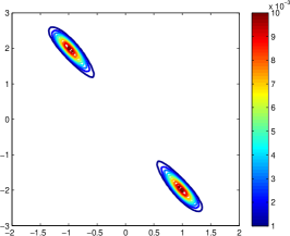
Refer to caption Refer to caption Refer to caption
(1) True Posterior (2) SGD NPV (3) One-pass SMC
Refer to caption Refer to caption Refer to caption
(4) Gibbs Sampling (5) SGD Langevin (6) SVI
Figure 3: Visualization of posteriors of mixture model on synthetic dataset obtained by several inference methods.

We use the normalized Gaussian kernel in this experiment. For one-pass SMC, we use the suggested kernel bandwidth in [3]. For our method, since we increase the samples, the kernel bandwidth is shrunk in rate of O(m12)𝑂superscript𝑚12O(m^{-\frac{1}{2}}) as the theorem suggested. The batch size for stochastic algorithms and one-pass SMC is set to be 101010. The total number of particles for the Monte Carlo based competitors, i.e., SMC, SGD Langevin, Gibbs sampling, and our method is 150015001500 in total. We also keep 150015001500 Gaussian components in SGD NPV. The burn-in period for Gibbs sampling and stochastic Langevin dynamics are 505050 and 100010001000 respectively.

The visualization of 101010 runs average posteriors obtained by the alternative methods are plotted in Figure 3. From these figures, we could have a direct understand about the behaviors for each competitors. The Gibbs sampling and stochastic gradient Langevin dynamics sampling stuck in one local mode in each run. Gibbs sampler could fit one of the contour quite well, better than the stochastic Langevin dynamics. It should be noticed that this is the average solution, the two contours in the result of stochastic gradient Langevin dynamics did not mean it finds both modes simultaneously. The one-pass sequential Monte Carlo and stochastic nonparametric variational inference are able to location multiple modes. However, their shapes are not as good as ours. Because of the multiple modes and the highly dependent variables in posterior, the stochastic variational inference fails to converge to the correct modes.

To compare these different kinds of algorithms in a fair way, we evaluate their performances using total variation and cross entropy of the solution against the true potential functions versus the number of observations visited. In order to evaluate the total variation and the cross entropy between the true posterior and the estimated one, we use both kernel density estimation and Gaussian estimation to approximate the posterior density and report the better one for Gibbs sampling and stochastic Langevin dynamics. The kernel bandwidth is set to be 0.10.10.1 times the median of pairwise distances between data points (median trick).

In Figure 1(3)(4), the one-pass SMC performs similar to our algorithm at beginning. However, it cannot utilize the dataset effectively, therefore, it stopped with high error. It should be noticed that the one-pass SMC starts with more particles while our algorithm only requires the same number of particles at final stage. The reason that Gibbs sampling and the stochastic gradient Langevin dynamics perform worse is that they stuck in one mode. It is reasonable that Gibbs sampling fits the single mode better than stochastic gradient Langevin dynamics since it generates one new sample by scanning the whole dataset. For the stochastic nonparametric variational inference, it could locate both modes, however, it optimizes a non-convex objective which makes its variance much larger than our algorithm. The stochastic variational inference fails because of the highly dependent variables and multimodality in posterior.

H.2 Bayesian Logistic Regression

The likelihood function is

p(y|x,w)=11+exp(ywx)𝑝conditional𝑦𝑥𝑤11𝑦superscript𝑤top𝑥p(y|x,w)=\frac{1}{1+\exp(-yw^{\top}x)}

with w𝑤w as the latent variables. We use Gaussian prior for w𝑤w with identity covariance matrix.

We first reduce the dimension to 505050 by PCA. The batch size is set to be 100100100 and the step size is set to be 1100+t1100𝑡\frac{1}{100+\sqrt{t}}. We stop the stochastic algorithms after they pass through the whole dataset 555 times. The burn-in period for stochastic Langevin dynamic is set to be 100010001000. We rerun the experiments 101010 times.

Although the stochastic variant of nonparametric variational inference performs comparable to our algorithm with fewer components, its speed is bottleneck when applied to large-scale problems. The gain from using stochastic gradient is dragged down by using L-BFGS to optimize the second-order approximation of the evidence lower bound.

H.3 Sparse Gaussian Processes

H.3.1 1D Synthetic Dataset
Refer to caption Refer to caption Refer to caption Refer to caption
(1) Iteration 0 (2) Iteration 1 (3) Iteration 5 (4) Iteration 10
Refer to caption Refer to caption Refer to caption Refer to caption
(5) Iteration 20 (6) Iteration 50 (7) Iteration 80
(8)Posterior Convergence
Figure 4: Visualization of posterior prediction distribution. The red curve is the mean function and the pale red region is the variance of the posterior. The cyan curve the ground truth. The last one shows convergence of the posterior mean to the ground truth.

We test the proposed algorithm on 1D synthetic data. The data are generated by

y=3x2+(sin(3.53πx)+cos(7.7πx))exp(1.6π|x|)+0.1e𝑦3superscript𝑥23.53𝜋𝑥7.7𝜋𝑥1.6𝜋𝑥0.1𝑒y=3x^{2}+(\sin(3.53\pi x)+\cos(7.7\pi x))\exp(-1.6\pi|x|)+0.1e

where x[0.5,0.5]𝑥0.50.5x\in[-0.5,0.5] and e𝒩(0,1)similar-to𝑒𝒩01e\sim\mathcal{N}(0,1). The dataset contains 204820482048 observations which is small enough to run the exact GP regression. We use Gaussian RBF kernel in Gaussian processes and sparse Gaussian processes. Since we are comparing different inference algorithms on the same model, we use the same hyperparameters for all the inference algorithms. We set the kernel bandwidth σ𝜎\sigma to be 0.10.10.1 times the median of pairwise distances between data points (median trick), and β1=0.001superscript𝛽10.001\beta^{-1}=0.001. We set the stepsize in the form of ηn0+t𝜂subscript𝑛0𝑡\frac{\eta}{n_{0}+\sqrt{t}} for both PMD and SVI and the batch size to be 128128128. Figure. 4 illustrates the evolving of the posterior provided by PMD with 161616 particles and 128128128 inducing variables when the algorithms visit more and more data. To illustrate the convergence of the posterior provided by PMD, we initialize the 𝐮=0𝐮0\mathbf{u}=0 in PMD. Later, we will see we could make the samples in PMD more efficient.

H.3.2 Music Year Prediction

We randomly selected 463,715463715463,715 songs to train the model and test on 5,16351635,163 songs. As in [5], the year values are linearly mapped into [0,1]01[0,1]. The data is standardized before regression. Gaussian RBF kernel is used in the model. Since we are comparing the inference algorithms, for fairness, we fixed the model parameters for all the inference algorithms, i.e., the kernel bandwidth is set to be the median of pairwise distances between data points and the observations precision β1=0.01superscript𝛽10.01\beta^{-1}=0.01. We set the number of inducing inputs to be 210superscript2102^{10} and batch size to be 512512512. The stepsize for both PMD and SVI are in the form of ηn0+t𝜂subscript𝑛0𝑡\frac{\eta}{n_{0}+\sqrt{t}}. To demonstrate the advantages of PMD comparing to SMC, we initialize PMD with prior while SMC with the SoD solution. We rerun the experiments 101010 times. We use both 161616 particles in SMC and PMD. We stop the stochastic algorithms after they pass through the whole dataset 222 times.

H.4 Latent Dirichlet Allocation

Refer to caption Refer to caption Refer to caption
Figure 5: Several topics learnd by LDA with PMD

We fix the hyper-parameter α=0.1𝛼0.1\alpha=0.1, β=0.01𝛽0.01\beta=0.01, and K=100𝐾100K=100. The batchsize is set to be 100100100. We use stepsize ηn0+tκ𝜂subscript𝑛0superscript𝑡𝜅\frac{\eta}{n_{0}+{t}^{\kappa}} for PMD, stochastic variational inference and stochastic Riemannian Langevin dynamic. For each algorithm a grid-search was run on step-size parameters and the best performance is reported. We stop the stochastic algorithms after they pass through the whole dataset 555 times.

The log-perplexity was estimated using the methods discussed in [34] on a separate holdout set with 100010001000 documents. For a document xdsubscript𝑥𝑑x_{d} in holdout set, the perplexity is computed by

perp(xd|X,α,β)=exp(n=1Ndlogp(xdn|X,α,β)Nd)perpconditionalsubscript𝑥𝑑𝑋𝛼𝛽superscriptsubscript𝑛1subscript𝑁𝑑𝑝conditionalsubscript𝑥𝑑𝑛𝑋𝛼𝛽subscript𝑁𝑑\text{perp}(x_{d}|X,\alpha,\beta)=\exp\bigg{(}-\frac{\sum_{n=1}^{N_{d}}\log p(x_{dn}|X,\alpha,\beta)}{N_{d}}\bigg{)}

where

p(xdn|X,α,β)=𝔼θd,Φ[θdΦ,xdn].𝑝conditionalsubscript𝑥𝑑𝑛𝑋𝛼𝛽subscript𝔼subscript𝜃𝑑Φdelimited-[]superscriptsubscript𝜃𝑑topsubscriptΦsubscript𝑥𝑑𝑛\displaystyle p(x_{dn}|X,\alpha,\beta)=\mathbb{E}_{\theta_{d},\Phi}\bigg{[}\theta_{d}^{\top}\Phi_{\cdot,x_{dn}}\bigg{]}. (19)

We separate the documents in testing set into two non-overlapped parts, xdestimationsuperscriptsubscript𝑥𝑑estimationx_{d}^{\text{estimation}} and xdevaluationsuperscriptsubscript𝑥𝑑evaluationx_{d}^{\text{evaluation}}. We first evaluate the θdsubscript𝜃𝑑\theta_{d} based on the xdestimationsuperscriptsubscript𝑥𝑑estimationx_{d}^{\text{estimation}}. For different inference methods, we use the corresponding strategies in learning algorithm to obtain the distribution of θdsubscript𝜃𝑑\theta_{d} based on xdestimationsuperscriptsubscript𝑥𝑑estimationx_{d}^{\text{estimation}}. We evaluate p(xdn|X,α,β)𝑝conditionalsubscript𝑥𝑑𝑛𝑋𝛼𝛽p(x_{dn}|X,\alpha,\beta) on xdevaluationsuperscriptsubscript𝑥𝑑evaluationx_{d}^{\text{evaluation}} with the obtained distribution of θdsubscript𝜃𝑑\theta_{d}. Specifically,

p(xdnevaluation|X,α,β)=𝔼Φ|X,β𝔼θdevaluation|Φ,α,xdestimation[θdΦ,xdn]𝑝conditionalsuperscriptsubscript𝑥𝑑𝑛evaluation𝑋𝛼𝛽subscript𝔼conditionalΦ𝑋𝛽subscript𝔼conditionalsuperscriptsubscript𝜃𝑑evaluationΦ𝛼superscriptsubscript𝑥𝑑estimationdelimited-[]superscriptsubscript𝜃𝑑topsubscriptΦsubscript𝑥𝑑𝑛\displaystyle p(x_{dn}^{\text{evaluation}}|X,\alpha,\beta)=\mathbb{E}_{\Phi|X,\beta}\mathbb{E}_{\theta_{d}^{\text{evaluation}}|\Phi,\alpha,x_{d}^{\text{estimation}}}\bigg{[}\theta_{d}^{\top}\Phi_{\cdot,x_{dn}}\bigg{]}

For PMD, SMC and stochastic Langevin dynamics,

θdkevaluation=n=1Ndestimationδ(zdnkestimation=1)+αNdestimation+Kαsuperscriptsubscript𝜃𝑑𝑘evaluationsuperscriptsubscript𝑛1superscriptsubscript𝑁𝑑estimation𝛿superscriptsubscript𝑧𝑑𝑛𝑘estimation1𝛼superscriptsubscript𝑁𝑑estimation𝐾𝛼\displaystyle\theta_{dk}^{\text{evaluation}}=\frac{\sum_{n=1}^{N_{d}^{\text{estimation}}}\delta(z_{dnk}^{\text{estimation}}=1)+\alpha}{N_{d}^{\text{estimation}}+K\alpha}

For stochastic variational inference, q(θd)𝑞subscript𝜃𝑑q(\theta_{d}) is updated as in the learning procedure.

We illustrate several topics learned by LDA with our algorithm in Figure.5.