aainstitutetext: Max Planck Institute for Physics, Föhringer Ring 6, 80805 Munich, Germanybbinstitutetext: Department of Physics, Harvard University, Cambridge, MA 02138, USA

Strongly coupled phases of 𝒩=1𝒩1\mathcal{N}=1 S-duality

Iñaki García-Etxebarria b    and Ben Heidenreich inaki@mpp.mpg.de bjheiden@physics.harvard.edu
Abstract

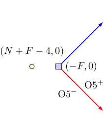
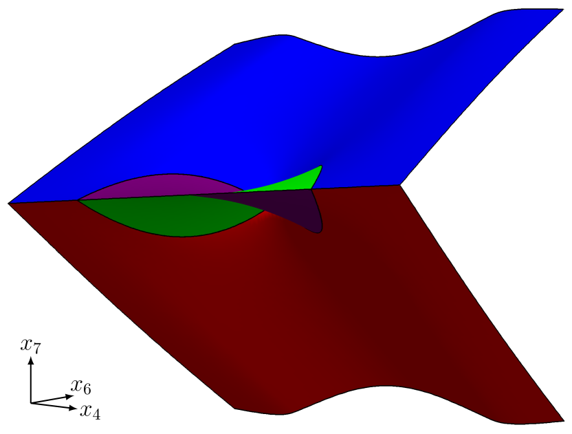
We analyze S-duality of orientifolds of the Calabi-Yau cone over the first del Pezzo surface (dP1𝑑subscript𝑃1dP_{1}). The S-duals of known phases, described by quiver gauge theories, contain intrinsically strongly-coupled sectors. These sectors are realized by a higher multiplicity intersection of NS5 branes and D5 branes atop an O5 plane, and can be thought of as stuck at the infinite coupling point between two Seiberg-dual gauge theories. We argue that such sectors appear generically in orientifolds of non-orbifold singularities, where in many examples every orientifold phase contains such a sector. Understanding such sectors is therefore key to understanding orientifolds of Calabi-Yau singularities. We construct the strongly-coupled sectors for dP1𝑑subscript𝑃1dP_{1} orientifolds using deconfinement, and show that they have interesting, non-trivial properties. Using this construction, we verify the predictions of S-duality for dP1𝑑subscript𝑃1dP_{1}.

1 Introduction

S-duality, where two dual theories are related by an exactly marginal deformation, is a ubiquitous phenomenon in theories with extended supersymmetry. Perhaps the most elegant example is Montonen-Olive duality in 𝒩=4𝒩4\mathcal{N}=4 gauge theories, which exchanges electric and magnetic fields and replaces the gauge group with its Langlands dual. A subclass of these dualities admit a simple embedding in string theory as the self-duality of the world-volume gauge theory on D3 branes induced by S-duality in type IIB string theory, as well as the various dualities which arise when the D3 branes are coincident with an O3 plane. The latter case was concisely described by Witten:1998xy , where it was shown that the O3 plane type is characterized in the gravity dual by a pair of discrete holonomies (hereafter referred to as discrete torsion) for the RR and NSNS two-form potentials, and that the S-dualities between the corresponding gauge theories are explained by the well-known action of type IIB S-duality on these potentials.

There are a number of ways that S-duality can be realized in 𝒩=1𝒩1\mathcal{N}=1 gauge theories. It occurs in mass deformations of S-dual theories with extended supersymmetry Leigh:1995ep ; Argyres:1999xu as well as in 𝒩=1𝒩1\mathcal{N}=1 gaugings of Gaiotto dualities Benini:2009mz . The distinct phenomenon of universality, where two theories are related by renormalization group flow, is ubiquitous in 𝒩=1𝒩1\mathcal{N}=1 gauge theories Seiberg:1994pq ; Seiberg:1995ac , and bears some relation to S-dualities in theories with extended supersymmetry Leigh:1995ep .

Another manifestation of 𝒩=1𝒩1\mathcal{N}=1 S-duality occurs in the chiral world-volume gauge theory on D3 branes probing a Calabi-Yau singularity dualities1 ; Bianchi:2013gka ; dualities2 , analogous the realization of Montonen-Olive duality on D3 branes in a flat background.111𝒩=0𝒩0\mathcal{N}=0 generalizations of these dualities have also been argued to exist Uranga:1999ib ; Sugimoto:2012rt ; Hook:2013vza . As in the 𝒩=4𝒩4\mathcal{N}=4 case, the dual theories correspond to different weakly-coupled “cusps” along the same fixed line, where gs0subscript𝑔𝑠0g_{s}\to 0 in some dual description of the parent string theory. The addition of orientifold planes leads to non-zero beta functions near the cusp, hence the infrared fixed point is interacting and there is a non-trivial relationship between the dynamics at distinct dual cusps.222Even in the infrared of these orientifold gauge theories, the gs=0subscript𝑔𝑠0g_{s}=0 cusp is a distinguished point along the fixed line, where (depending on the theory) there are enhanced global symmetries and/or free vector multiplets.

These S-dualities are distinguished by their chiral, intrinsically 𝒩=1𝒩1\mathcal{N}=1 nature333See also Gaiotto:2015usa ; Franco:2015jna ; Hanany:2015pfa for some recent work on chiral 𝒩=1𝒩1\mathcal{N}=1 S-dualities arising from compactifications of 6d (1,0)10(1,0) theories. and their rich infrared dynamics near the cusp, with examples exhibiting confinement, chiral symmetry breaking, and a dynamically generated superpotential. Moreover, they provide an important cross-check on the physics of Calabi-Yau orientifold singularities — where the S-dualities originate from the SL(2,)𝑆𝐿2SL(2,\mathbb{Z}) self-duality of type IIB string theory — a role which will prove to be crucial in the present paper.

In dualities2 , a systematic understanding of S-dualities arising in orientifolds of isolated orbifold singularities was obtained by repeating the analysis of discrete torsion in Witten:1998xy for these geometries. In this class of theories, the pattern of S-dualities predicted by string theory is reproduced perfectly in the dual gauge theories, passing all available checks.

However, applying the same arguments to more general isolated singularities immediately gives rise to a conundrum. The geometry allows for additional discrete torsions, yet the number of known dual gauge theories is insufficient to fill out all the possible choices of torsion, and moreover these gauge theories do not fill out complete SL(2,)𝑆𝐿2SL(2,\mathbb{Z}) multiplets, a problem which was recognized in dualities1 for perhaps the simplest non-orbifold example, the Calabi-Yau cone over the first del Pezzo surface (dP1𝑑subscript𝑃1dP_{1}). The problem is worse still for the higher del Pezzo singularities, where for most orientifold involutions no dual gauge theory is known Franco:2010jv , despite the rapidly growing set of discrete torsions. Other non-orbifold singularities exhibit similar problems.

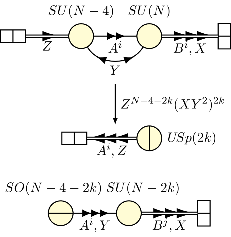
In this paper, we resolve this puzzle for the dP1𝑑subscript𝑃1dP_{1} singularity, developing techniques which will generalize to other cases. We find that there are more orientifold phases than previously known, with the new phases precisely filling out the allowed discrete torsions. The new phases consist of a quiver gauge theory coupled to an intrinsically strongly-coupled sector, dual to a higher multiplicity intersection of NS5 and D5 branes atop an O5 plane. We describe this strongly-coupled sector via deconfinement Berkooz:1995km ; Pouliot:1995me , which produces a large collection of quiver gauge theories in the same universality class as it. This sector exhibits novel behavior, such baryons transforming in the spinor representation of an SO(2N)𝑆𝑂2𝑁SO(2N) flavor symmetry which emerges accidentally in the gauge theory description.

These new sectors can be thought of as arising at the midpoint of a Seiberg duality, where the presence of an orientifold plane prevents a deformation to one or the other of the Seiberg-dual descriptions, trapping the theory at strong coupling. We argue that these sectors occur in certain orientifold phases of every toric non-orbifold singularity, including those with trivial discrete torsion. For most orientifold involutions of more complicated isolated singularities such as cones over the higher del Pezzo surfaces, every phase includes a strongly coupled sector, explaining the lack of known gauge theory duals.

Combining the strongly-coupled sector with known ingredients, we obtain a list of theories describing the dP1𝑑subscript𝑃1dP_{1} orientifold which is in complete agreement with the discrete torsion classification, and which exhibits the S-dualities predicted by that classification, including but generalizing the dP1𝑑subscript𝑃1dP_{1} duality found in dualities1 . We test these dualities by computing the superconformal index for all the phases, including those involving the strongly-coupled sector. We find that the theories predicted to be S-dual have indices which match for a large number of low-lying states (limited only by computational power), whereas theories not predicted to be S-dual have distinct indices.

Our paper is organized as follows. In §2, we describe a class of del Pezzo orientifolds, including our main focus, the dP1𝑑subscript𝑃1dP_{1} orientifold. We then summarize the known gauge theory duals and classify the available discrete torsions, highlighting the mismatch between the two. In §3, we determine the discrete torsions of the known dP1𝑑subscript𝑃1dP_{1} orientifold gauge theories by partially resolving to the dP0𝑑subscript𝑃0dP_{0} orientifold singularity studied in dualities1 ; dualities2 plus an O3 plane. We compare this torsion classification with a brane tiling construction of the orientifold, suggesting that the missing theories contain a sector dual to a higher-multiplicity intersection of NS5 branes atop a stack of D5 branes, frozen in place by an O5 plane. We then comment on the expected properties of these strongly-coupled “quad CFT” sectors. In §4, we obtain a gauge-theory description of the quad-CFTs by engineering deconfinement in the brane tiling, resolving the higher-multiplicity intersection. In the process, extra information is uncovered (in the form of flavor branes in the deconfined theory) which is crucial to reproducing the RR discrete torsion in the gravity dual. We describe some novel properties of the quad CFTs and compare their behavior with our expectations, providing non-trivial evidence that our description is correct. Finally, in §5 we apply the deconfinement construction of the quad CFTs to describe the missing phases of the dP1𝑑subscript𝑃1dP_{1} orientifold. We verify that the new theories neatly fill out the missing discrete torsions, and provide highly non-trivial evidence that the predicted S-dualities are realized in these theories, based on comparing the superconformal indices between the various phases. We conclude in §6.

Appendix A contains a brief review of the geometry of del Pezzo singularities, appendix B gives a microscopic description of the previously-known phases of dP1𝑑subscript𝑃1dP_{1} in terms of exceptional collections, useful for determining the brane charges, and appendix C summarizes some of our explicit results for the superconformal indices of all phases of the dP1𝑑subscript𝑃1dP_{1} orientifold.

2 Del Pezzo orientifolds

In this section, we construct a simple class of orientifold singularities and explore their properties.

2.1 The orientifold geometry

The Calabi-Yau cone over the first del Pezzo surface (dP1𝑑subscript𝑃1dP_{1}) is the toric variety described by the following gauged linear sigma model (GLSM, see Witten:1993yc for an introduction):

z1z2z3z4tU(1)a10113U(1)b01012missing-subexpressionsubscript𝑧1subscript𝑧2subscript𝑧3subscript𝑧4𝑡missing-subexpressionmissing-subexpressionmissing-subexpressionmissing-subexpressionmissing-subexpressionmissing-subexpression𝑈subscript1𝑎10113𝑈subscript1𝑏01012\begin{array}[]{c|ccccc}&z_{1}&z_{2}&z_{3}&z_{4}&t\\ \hline\cr U(1)_{a}&1&0&1&1&-3\\ U(1)_{b}&0&1&0&1&-2\end{array} (1)

subject to the D-term conditions

|z1|2+|z3|2+|z4|23|t|2=ξa,|z2|2+|z4|22|t|2=ξb,|z_{1}|^{2}+|z_{3}|^{2}+|z_{4}|^{2}-3|t|^{2}=\xi_{a}\qquad,\qquad|z_{2}|^{2}+|z_{4}|^{2}-2|t|^{2}=\xi_{b}\;, (2)

where the Fayet-Iliopoulos (FI) parameters ξasubscript𝜉𝑎\xi_{a} and ξbsubscript𝜉𝑏\xi_{b} control the resolutions of the singularity. For ξa>ξb>0subscript𝜉𝑎subscript𝜉𝑏0\xi_{a}>\xi_{b}>0 the exceptional divisor t=0𝑡0t=0 is dP1𝑑subscript𝑃1dP_{1}, and the O3/O7 involution tt𝑡𝑡t\to-t describes an O7 plane wrapping this divisor.

We now generalize this construction to the other del Pezzo surfaces. Let KΣsubscript𝐾ΣK_{\Sigma} denote the canonical bundle of a smooth divisor ΣΣ\Sigma embedded in a smooth Calabi-Yau threefold Y𝑌Y. We have GriffithsHarris

KΣ=KY|ΣNΣsubscript𝐾Σtensor-productevaluated-atsubscript𝐾𝑌Σsubscript𝑁ΣK_{\Sigma}=\left.K_{Y}\right|_{\Sigma}\otimes N_{\Sigma} (3)

where NΣsubscript𝑁ΣN_{\Sigma} is the normal bundle of ΣYΣ𝑌\Sigma\subset Y, and KYsubscript𝐾𝑌K_{Y} is the canonical bundle of Y𝑌Y. The Calabi-Yau condition implies that KYsubscript𝐾𝑌K_{Y} is trivial, hence KΣ=NΣsubscript𝐾Σsubscript𝑁ΣK_{\Sigma}=N_{\Sigma}. Thus, the local embedding of ΣΣ\Sigma in Y𝑌Y is isomorphic to the canonical bundle KΣsubscript𝐾ΣK_{\Sigma} on ΣΣ\Sigma, and is independent of the global structure of Y𝑌Y.

Locally, we can always construct an involution σ:YY:𝜎𝑌𝑌\sigma:Y\to Y by reflecting the fibers of NΣsubscript𝑁ΣN_{\Sigma} (\mathbb{C}\to-\mathbb{C}). σ𝜎\sigma is holomorphic by construction with an isolated fixed plane ΣΣ\Sigma, and corresponds to wrapping an O7 plane on ΣΣ\Sigma.444Unless ΣΣ\Sigma is a K3 surface or T4superscript𝑇4T^{4}, NΣsubscript𝑁ΣN_{\Sigma} must be non-trivial, hence tadpole cancellation requires the presence of D7 branes intersecting or wrapping ΣΣ\Sigma. To avoid “flavor” D7 branes, we assume that four D7 branes wrap ΣΣ\Sigma, cancelling the C0subscript𝐶0C_{0} charge of the O7 plane. As above, the local geometry is independent of the global structure of Y𝑌Y, though σ𝜎\sigma may or may not extend to a globally defined holomophic involution, depending on Y𝑌Y.

Let [Σ]H(1,1)(Y)delimited-[]Σsuperscript𝐻11𝑌[\Sigma]\in H^{(1,1)}(Y) denote the divisor class of ΣΣ\Sigma. If [Σ]delimited-[]Σ-[\Sigma] is a positive class then there is a corresponding Kähler modulus of Y𝑌Y with ΣΣ\Sigma as the exceptional divisor. In this case, the adjunction formula implies that KΣ=NΣsubscript𝐾Σsubscript𝑁Σ-K_{\Sigma}=-N_{\Sigma} is ample, hence ΣΣ\Sigma is a del Pezzo surface: either 2superscript2\mathbb{P}^{2} blown up at k𝑘k generic points (0k80𝑘80\leq k\leq 8) — denoted dPk𝑑subscript𝑃𝑘dP_{k} — or the zeroth Hirzebruch surface, 𝔽01×1subscript𝔽0superscript1superscript1\mathbb{F}_{0}\cong\mathbb{P}^{1}\times\mathbb{P}^{1}.

For each of these ten cases, we can construct an affine cone by setting the corresponding Kähler modulus of Y𝑌Y to zero and reading off the local geometry YpYsubscript𝑌𝑝𝑌Y_{p}\subset Y near the singular point p𝑝p. An orientifold Xp=Yp/σsubscript𝑋𝑝subscript𝑌𝑝𝜎X_{p}=Y_{p}/\sigma can be constructed using the involution described above, where p𝑝p is an isolated fixed point of σ𝜎\sigma.555The affine varieties Ypsubscript𝑌𝑝Y_{p} and Xpsubscript𝑋𝑝X_{p} depend only on the choice of del Pezzo surface — and on the 2k82𝑘82k-8 complex structure moduli of dPk𝑑subscript𝑃𝑘dP_{k} for k5𝑘5k\geq 5 — and not on the global details of Y𝑌Y. However, all ten singularities admit global embeddings, see e.g. Malyshev:2007yb , where σ𝜎\sigma can be defined globally by ww𝑤𝑤w\to-w in the notation of that paper. For completeness, concrete geometric realizations of all ten varieties and their orientifolds are presented in appendix A.

2.2 Known gauge theory constructions

We now present the known gauge theory duals of D3 branes probing the orientifold singularities described in the previous subsection. These are only known for the dP0𝑑subscript𝑃0dP_{0}, dP1𝑑subscript𝑃1dP_{1} and 𝔽0subscript𝔽0\mathbb{F}_{0} orientifold singularities, and we later argue that this list is incomplete even in the dP1𝑑subscript𝑃1dP_{1} and 𝔽0subscript𝔽0\mathbb{F}_{0} cases.

We begin with the toric cases: dPk𝑑subscript𝑃𝑘dP_{k} for k3𝑘3k\leq 3 and 𝔽0subscript𝔽0\mathbb{F}_{0}. In these cases, we can use the dimer model technology developed in Hanany:2005ve ; Franco:2005rj and the orientifold rules laid out in Franco:2007ii to derive the gauge theories corresponding to these orientifold singularities. We briefly review the required tools, referring the interested reader to the extensive literature (see e.g. Kennaway:2007tq ; Yamazaki:2008bt and references therein) for further details.

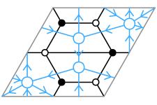
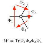
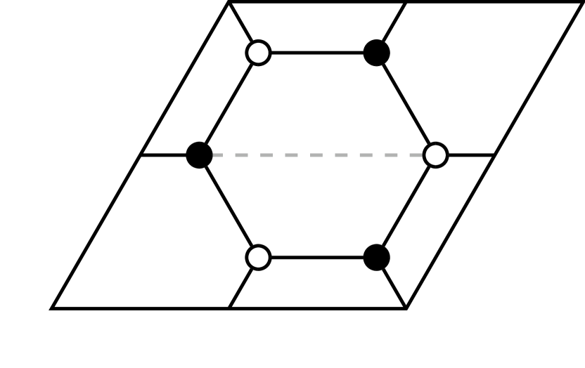
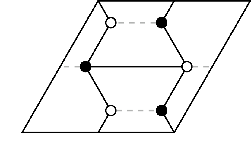
As illustrated in figure 1, a dimer model is a bipartite graph embedded on the torus such that the surface of the torus is divided into contractible faces by the edges of the graph.666More technically, we are only interested in “non-degenerate” dimers, in the sense of Ishii:2007 . Other “consistency” conditions are often imposed (see e.g. Hanany:2005ss ), but we will not do so for reasons which become clear in §4. A dimer model corresponds to a quiver gauge theory by graph dualization: each face of the dimer model corresponds to a node in the quiver, and each edge to an arrow in the quiver, oriented so that the arrows circulate clockwise (counterclockwise) around the white (black) vertices of the bipartite graph. The vertices encode the superpotential: the loop in the quiver surrounding each white (black) vertex corresponds to a term in the superpotential with coefficient +11+1 (11-1).

Refer to caption
(a) A dimer model and its dual quiver.
Refer to caption
(b) Reading off W𝑊W.
Refer to caption
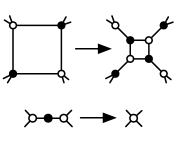
(c) Seiberg duality in the dimer.
Figure 1: 1(a) A dimer model (black) and its dual quiver (blue). This dimer corresponds to the dP1𝑑subscript𝑃1dP_{1} singularity. 1(b) Each vertex in the dimer represents a superpotential term. 1(c) Seiberg duality (top) and integrating out (bottom) have a graphical interpretation in the dimer.

The mesonic moduli space of this quiver gauge theory is a toric Calabi-Yau singularity which can be read off using the forward algorithm Feng:2000mi ; Franco:2005rj . Conversely, for each toric Calabi-Yau singularity, one or more dimer models can be constructed using the inverse algorithm Feng:2000mi ; Hanany:2005ss . When more than one dimer model is obtainable using the inverse algorithm, these toric phases are related to each other by Seiberg duality Beasley:2001zp , which takes the form of “urban renewal” in the dimer Franco:2005rj , see figure 1(c).

The quiver gauge theories obtained by the inverse algorithm describe the infrared of the worldvolume gauge theory on D3 branes probing the toric singularity in question. dP0𝑑subscript𝑃0dP_{0} (figure 2(a)) and dP1𝑑subscript𝑃1dP_{1} (figure 1(a)) each have a single toric phase, whereas 𝔽0subscript𝔽0\mathbb{F}_{0} (figures 2(b)-2(c)) and dP2𝑑subscript𝑃2dP_{2} (figure 3(a)) have two phases each, and dP3𝑑subscript𝑃3dP_{3} (figure 3(b)) has four phases.

Refer to caption
(a) dP0𝑑subscript𝑃0dP_{0}
Refer to caption
(b) 𝔽0subscript𝔽0\mathbb{F}_{0} phase I
Refer to caption
(c) 𝔽0subscript𝔽0\mathbb{F}_{0} phase II
Figure 2: Dimer models for 2(a) dP0𝑑subscript𝑃0dP_{0}, 2(b) 𝔽0subscript𝔽0\mathbb{F}_{0} phase I, and 2(c) 𝔽0subscript𝔽0\mathbb{F}_{0} phase II. The dimer for dP1𝑑subscript𝑃1dP_{1} is shown in figure 1(a).
Refer to caption
(a) dP2𝑑subscript𝑃2dP_{2} phases
Refer to caption
(b) dP3𝑑subscript𝑃3dP_{3} phases
Figure 3: Dimer models for 3(a) dP2𝑑subscript𝑃2dP_{2} and 3(b) dP3𝑑subscript𝑃3dP_{3}.

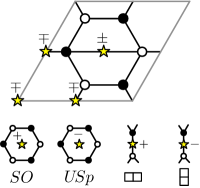
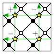
Following Franco:2007ii , we can construct the worldvolume gauge theory on D3 branes probing an orientifold of a toric singularity by orientifolding the dimer model itself. The geometric involution considered above preserves all the isometries of the toric singularity, so that the quotient space is also toric. Geometric involutions of this type correspond to involutions of the dimer model with four isolated fixed points mapping white nodes to black nodes and vice versa. Each fixed point has an associated sign, or “T-parity” Imamura:2008fd , subject to the requirement that the product of all four T-parities is positive (negative) when the number of white vertices in the dimer is even (odd). A (generalized) quiver gauge theory can be read off as before, where now each face and its image corresponds to a single SU(n)𝑆𝑈𝑛SU(n) gauge group, each edge and its image to a single matter multiplet, and each vertex and its image to a single superpotential term.777The sign of the coefficient is no longer important. When a face is mapped to itself, it corresponds to an SO𝑆𝑂SO (USp𝑈𝑆𝑝U\!Sp) gauge group if the enclosed fixed point is positive (negative), whereas an edge mapped to itself corresponds to symmetric (antisymmetric) tensor matter if the fixed point it crosses is positive (negative), see figure 4(a).

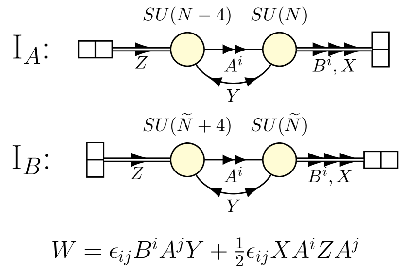
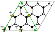
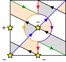
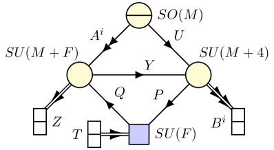
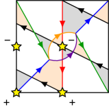
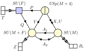
We consider dP1𝑑subscript𝑃1dP_{1} first.888The dP1𝑑subscript𝑃1dP_{1} and 𝔽0subscript𝔽0\mathbb{F}_{0} orientifold gauge theories derived below were first written down in dualities1 . The dP0𝑑subscript𝑃0dP_{0} orientifold theories have been known much longer Angelantonj:1996uy ; Lykken:1997ub ; Kakushadze:1998tr . The corresponding dimer model is shown in figure 1(a). Up to the choice of fixed point signs, a single fixed-point involution is possible. The relative signs of the fixed points can be fixed by the requirement that the SU(2)×U(1)𝑆𝑈2𝑈1SU(2)\times U(1) isometry of dP1𝑑subscript𝑃1dP_{1} is unbroken, giving two distinct orientifolds, which we call IAsubscriptI𝐴\mathrm{I}_{A} and IBsubscriptI𝐵\mathrm{I}_{B}. The orientifolded dimer model is shown in figure 4(a), and the resulting quivers and superpotential are displayed in figure 4(b) using the generalized quiver notation defined in figure 5. The dP0𝑑subscript𝑃0dP_{0} orientifold studied in dualities1 ; dualities2 can be obtained from here by Higgsing the tensor Z𝑍Z.

Refer to caption
(a) dP1𝑑subscript𝑃1dP_{1} orientifold and dictionary.
Refer to caption
(b) dP1𝑑subscript𝑃1dP_{1} quiver and superpotential.
Figure 4: 4(a) (top) Orientifolds of the dP1𝑑subscript𝑃1dP_{1} dimer model which preserve the SU(2)×U(1)𝑆𝑈2𝑈1SU(2)\times U(1) isometry of dP1𝑑subscript𝑃1dP_{1}. (bottom) The orientifold gauge theory can be read off from the dimer using this dictionary. 4(b) Quivers for the dP1𝑑subscript𝑃1dP_{1} orientifolds, where A𝐴A (B𝐵B) corresponds to the upper (lower) choice of fixed point signs in 4(a). Our notation for quivers is explained in figure 5.
Refer to caption
Figure 5: Summary of our quiver notation. Reversing the directions of the arrows corresponds to taking the charge conjugate of the representation, and multiple arrowheads in the same direction indicate multiple fields in the same representation.

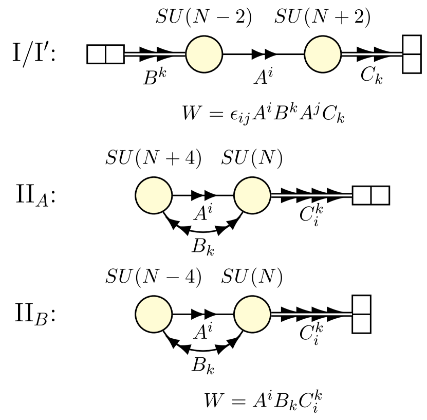
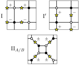
For 𝔽0subscript𝔽0\mathbb{F}_{0}, there are two toric phases to consider. In phase I, two different involutions are possible, but they are related to each other by rotating the dimer model by 90superscript9090^{\circ}, exchanging the two 1superscript1\mathbb{P}^{1} factors. As above, the relative signs of the fixed points can be fixed by requiring that the SU(2)×SU(2)𝑆𝑈2𝑆𝑈2SU(2)\times SU(2) isometry of 𝔽01×1subscript𝔽0superscript1superscript1\mathbb{F}_{0}\cong\mathbb{P}^{1}\times\mathbb{P}^{1} is unbroken, whereas the two remaining choices are related by translating the torus by half a period, hence they are equivalent. In phase II, only one involution is possible, but the two sign choices consistent with the SU(2)×SU(2)𝑆𝑈2𝑆𝑈2SU(2)\times SU(2) isometry are not equivalent, giving two distinct orientifold theories, IIA and IIB. However, unlike phases IA and IB of dP1𝑑subscript𝑃1dP_{1} or dP0𝑑subscript𝑃0dP_{0}, IIA and IIB are related by Seiberg duality, and therefore lie in the same universality class. The orientifolded dimers are shown in figure 6(a) and the resulting quiverfolds and superpotentials in figure 6(b).
Refer to caption
(a) 𝔽0subscript𝔽0\mathbb{F}_{0} orientifolds.
Refer to caption
(b) Orientifold quivers and superpotentials.
Figure 6: 6(a) Orientifolds of 𝔽0subscript𝔽0\mathbb{F}_{0} phase I and phase II, where IIA (IIB) corresponds to the upper (lower) choice of fixed point signs. The orientifolds I and I are related by a rotation of the dimer model, which generates an outer automorphism of the global symmetry group of the corresponding gauge theory. 6(b) Quivers for the 𝔽0subscript𝔽0\mathbb{F}_{0} orientifolds. The orientifolds I and I give identical gauge theories up to the labeling of the global symmetries. The orientifolds IIA and IIB are Seiberg duals.

The higher del Pezzos dP2𝑑subscript𝑃2dP_{2} and dP3𝑑subscript𝑃3dP_{3} are strikingly different. In these cases, no fixed-point involutions are possible in any toric phase Franco:2010jv ! For instance, dP2𝑑subscript𝑃2dP_{2} phase II and dP3𝑑subscript𝑃3dP_{3} phases III and IV each have a unique largest face with either 888 or 121212 sides. The involution must map this face to itself, but this is incompatible with the rule that white vertices are mapped to black vertices, so no fixed-point involution exists for these phases. Likewise, dP2𝑑subscript𝑃2dP_{2} phase I and dP3𝑑subscript𝑃3dP_{3} phase I each have a black vertex with valence 555 or 666 and no white vertices with valence greater than four, once again violating the rule that white vertices are mapped to black vertices. By contrast, dP3𝑑subscript𝑃3dP_{3} phase II admits a unique involution that exchanges white and black vertices, but this involution — a horizontal translation by half a period — has no fixed points and breaks the toric isometries, hence it cannot correspond to one of the orientifolds considered above. In fact, as shown in §3.2, the absence of fixed-point involutions for these theories generalizes to a broad class of isolated toric singularities, and is one of the central mysteries that we aim to address in this work.

We comment briefly on the non-toric cases, dPk𝑑subscript𝑃𝑘dP_{k} for 4k84𝑘84\leq k\leq 8. In these cases, the toric technology of Franco:2005rj ; Franco:2007ii is unavailable, though quivers and superpotentials for the parent gauge theory are known Wijnholt:2002qz , and — following Wijnholt:2007vn (see also dualities1 ) — we can in principle orientifold these quivers to obtain the orientifold gauge theories of interest.999One can show that in the toric case the approaches of Wijnholt:2007vn and Franco:2007ii are equivalent BJHorientifoldnote . However, since there are an infinite number of Seiberg-dual quivers to orientifold, a systematic approach may not be possible.101010It may be that only a finite number of quivers admit an involution. It would be interesting to explore this further. Instead, we consider a few examples to illustrate the difficulties which arise.

The dPk𝑑subscript𝑃𝑘dP_{k} for k5𝑘5k\geq 5 have 2k82𝑘82k-8 complex structure moduli, none of which are projected out by the orientifold considered above, and we expect that the correct gauge theory dual will have corresponding exactly marginal deformations. (These appear as superpotential deformations in the unorientifolded quivers of Wijnholt:2002qz .) For dP5𝑑subscript𝑃5dP_{5} and dP6𝑑subscript𝑃6dP_{6} there are points in complex structure moduli space where the del Pezzo surface degenerates and the del Pezzo singularity becomes a non-isolated toric singularity. For instance, the cubic XYZW3=0𝑋𝑌𝑍superscript𝑊30XYZ-W^{3}=0 — equivalent to the orbifold singularity 3/(3×3)superscript3subscript3subscript3\mathbb{C}^{3}/(\mathbb{Z}_{3}\times\mathbb{Z}_{3}) via the embedding X=x3𝑋superscript𝑥3X=x^{3}, Y=y3𝑌superscript𝑦3Y=y^{3}, Z=z3𝑍superscript𝑧3Z=z^{3}, W=xyz𝑊𝑥𝑦𝑧W=xyz — is a degeneration of the dP6𝑑subscript𝑃6dP_{6} singularity and the complete intersection of quadrics Z2=XY=UVsuperscript𝑍2𝑋𝑌𝑈𝑉Z^{2}=XY=UV — equivalent to a 2×2subscript2subscript2\mathbb{Z}_{2}\times\mathbb{Z}_{2} orbifold of the conifold via the embedding X=x2𝑋superscript𝑥2X=x^{2}, Y=y2𝑌superscript𝑦2Y=y^{2}, U=u2𝑈superscript𝑢2U=u^{2}, V=v2𝑉superscript𝑣2V=v^{2} and Z=xyuv𝑍𝑥𝑦𝑢𝑣Z=xyuv — is a degeneration of the dP5𝑑subscript𝑃5dP_{5} singularity. There is also a degeneration of the dP5𝑑subscript𝑃5dP_{5} singularity which is a partial resolution of 3/(3×3)superscript3subscript3subscript3\mathbb{C}^{3}/(\mathbb{Z}_{3}\times\mathbb{Z}_{3}).

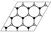
Since there are points in moduli space where the Calabi-Yau is toric, it may be possible to construct the gauge theory dual of the orientifold at these points using dimer models, and then to generalize the result by deforming it. For instance, the dimer model for 3/(3×3)superscript3subscript3subscript3\mathbb{C}^{3}/(\mathbb{Z}_{3}\times\mathbb{Z}_{3}) is shown in figure 7(a). The entire complex structure moduli space of dP6𝑑subscript𝑃6dP_{6} can be reproduced in the parent theory with a general superpotential, whereas the toric superpotential encoded by the dimer corresponds to one point in that moduli space (the degeneration given above). There is a unique involution of the dimer, with two possible choices of fixed-point signs which correspond to the desired geometric involution,111111Up to an overall sign, the fixed point signs are determined by the meson sign rules of Franco:2007ii . see figure 7(b).
Refer to caption
(a) Dimer for 3/(3×3)superscript3subscript3subscript3\mathbb{C}^{3}/(\mathbb{Z}_{3}\times\mathbb{Z}_{3}).
Refer to caption
(b) 3/(3×3)superscript3subscript3subscript3\mathbb{C}^{3}/(\mathbb{Z}_{3}\times\mathbb{Z}_{3}) orientifold.
Refer to caption
(c) 𝒞/(2×2)𝒞subscript2subscript2\mathcal{C}/(\mathbb{Z}_{2}\times\mathbb{Z}_{2}) orientifold.
Figure 7: 7(a) The dimer model for 3/3×3superscript3subscript3subscript3\mathbb{C}^{3}/\mathbb{Z}_{3}\times\mathbb{Z}_{3}, which is a toric degeneration of the dP6𝑑subscript𝑃6dP_{6} singularity. 7(b) An orientifold of 3/3×3superscript3subscript3subscript3\mathbb{C}^{3}/\mathbb{Z}_{3}\times\mathbb{Z}_{3} with fixed-point signs chosen to correspond to the del Pezzo orientifolds considered in the text. The green arrows represent cubic mesons which are projected out in the orientifold theory, obstructing the superpotential deformation required for generic complex structure moduli. 7(c) One toric phase of the 2×2subscript2subscript2\mathbb{Z}_{2}\times\mathbb{Z}_{2} orbifold of the conifold (which is a toric degeneration of the dP5𝑑subscript𝑃5dP_{5} singularity) and its orientifold. The green arrows represent quartic mesons which are projected out in the orientifold theory, obstructing deformation of the superpotential as above. The other toric phases are similar.

To deform these candidate orientifold theories, we modify the superpotential as in the parent theory. At a generic point in the moduli space of the parent theory, all 27 possible cubic superpotential terms are present Wijnholt:2002qz . However, not all of these terms can be switched on in the orientifold theory described above, as some mesons vanish identically, see figure 7(b). Thus, these gauge theories fail to describe the dP6𝑑subscript𝑃6dP_{6} singularity at a generic point in moduli space.121212It would be interesting to understand the string-theoretic interpretation of these orientifold theories, if any.

A similar story applies to the toric degenerations of dP5𝑑subscript𝑃5dP_{5}, see e.g. figure 7(c). While this does not rule out the possibility of obtaining the correct gauge theory dual by orientifolding one of the many Seiberg dual quivers describing these singularities, it does imply that this cannot be done for the “toric” phases of dP5𝑑subscript𝑃5dP_{5} and dP6𝑑subscript𝑃6dP_{6} (phases with equal rank nodes regardless of the superpotential), and the failure of the approach of Franco:2007ii for dP2𝑑subscript𝑃2dP_{2} and dP3𝑑subscript𝑃3dP_{3} already suggests that the solution to these problems lies elsewhere.

2.3 Discrete torsion in del Pezzo orientifolds

So far, we have made no distinction between different supersymmetric orientifolds with the same geometric involution. This is too naive — even in a flat background — because orientifold planes carry RR charges, and typically come in at least two variants (Op+superscript𝑝p^{+} and Opsuperscript𝑝p^{-} planes). In a curved background, orientifold planes may carry additional charges, and more than one orientifold plane can be hidden at a singularity, potentially leading to a large number of distinct orientifolds with the same geometric involution.

Fortunately, the AdS/CFT correspondence allows us to translate the difficult problem of classifying BPS orientifold planes at a singularity into the much easier one of classifying closed-string charges in the near-horizon geometry of the singularity, which is smooth if the singularity is isolated.

The idea, as in Witten:1998xy ; dualities1 ; dualities2 , is that distinct BPS O3/O7 orientifolds are distinguished by their RR and NSNS three-form charges, classified by H3(X5,~)superscript𝐻3subscript𝑋5~H^{3}(X_{5},\tilde{\mathbb{Z}}) where X5=Y5/σsubscript𝑋5subscript𝑌5𝜎X_{5}=Y_{5}/\sigma is the orientifolded horizon and ~~\tilde{\mathbb{Z}} denotes local cofficients, twisted by σ𝜎\sigma due to the projection σF3=F3superscript𝜎subscript𝐹3subscript𝐹3\sigma^{\ast}F_{3}=-F_{3}, σH3=H3superscript𝜎subscript𝐻3subscript𝐻3\sigma^{\ast}H_{3}=-H_{3}.131313A cohomology classification is sufficient for our present purposes Evslin:2006cj , and is able to reproduce the observed S-duality structure of the orientifold theories. A K-theoretic approach is difficult due in part to its unequal treatment of the RR and NSNS two-forms.

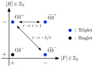
For instance, O3 planes in a flat background are classified by [F],[H]2delimited-[]𝐹delimited-[]𝐻subscript2[F],[H]\in\mathbb{Z}_{2} Witten:1998xy , where H3(S5/2,~)2superscript𝐻3superscript𝑆5subscript2~subscript2H^{3}(S^{5}/\mathbb{Z}_{2},\tilde{\mathbb{Z}})\cong\mathbb{Z}_{2} for the O3 involution zizisuperscript𝑧𝑖superscript𝑧𝑖z^{i}\to-z^{i} of 3superscript3\mathbb{C}^{3}, see figure 8. In this case, the NSNS torsion [H]delimited-[]𝐻[H] is trivial (nontrivial) for O3- (O3+) planes, whereas the RR torsion [F]delimited-[]𝐹[F] is trivial (nontrivial) for the O3- (O3~=O3+12D3superscript~O3superscriptO312D3\widetilde{\mathrm{O}3}^{-}=\mathrm{O3}^{-}+\frac{1}{2}\mathrm{\,D3}) variants, and likewise for the variants O3+ and O3~+superscript~O3\widetilde{\mathrm{O}3}^{+}. (The latter are perturbatively equivalent, being related by ττ+1𝜏𝜏1\tau\to\tau+1 in the SL(2,)𝑆𝐿2SL(2,\mathbb{Z}) self-duality group of type IIB string theory, but they differ in their nonperturbative spectra in the presence of D3 branes.) Orientifold planes of other codimensions can be classified in an analogous manner, see e.g. Hanany:2000fq .
Refer to caption
Figure 8: O3 planes are classified by the RR and NSNS torsion classes [F]delimited-[]𝐹[F] and [H]delimited-[]𝐻[H] in H3(S5/2,~)2superscript𝐻3superscript𝑆5subscript2~subscript2H^{3}(S^{5}/\mathbb{Z}_{2},\tilde{\mathbb{Z}})\cong\mathbb{Z}_{2}. The known action of SL(2,)𝑆𝐿2SL(2,\mathbb{Z}) on the RR and NSNS three-forms F3subscript𝐹3F_{3} and H3subscript𝐻3H_{3} dictates its action on the O3 plane variants.

In the remainder of this section, we compute the twisted homology groups Hi(X5,~)subscript𝐻𝑖subscript𝑋5~H_{i}(X_{5},\tilde{\mathbb{Z}}) for the del Pezzo orientifolds considered above. This determines H3(X5,~)superscript𝐻3subscript𝑋5~H^{3}(X_{5},\tilde{\mathbb{Z}}) by Poincare duality, and will help to clarify where the gaps in the collection of known field theory duals enumerated in the previous section lie.

Our calculation is based upon the long exact sequence AT :

Hi(X,~)Hi(Y,)piHi(X,)Hi1(X,~)subscript𝐻𝑖𝑋~subscript𝐻𝑖𝑌superscriptsubscript𝑝𝑖subscript𝐻𝑖𝑋subscript𝐻𝑖1𝑋~\ldots\longrightarrow H_{i}(X,\tilde{\mathbb{Z}})\longrightarrow H_{i}(Y,\mathbb{Z})\;\overset{p_{\ast}^{i}}{\longrightarrow}\;H_{i}(X,\mathbb{Z})\longrightarrow H_{i-1}(X,\tilde{\mathbb{Z}})\longrightarrow\ldots (4)

where X=Y/σ𝑋𝑌𝜎X=Y/\sigma, and pisuperscriptsubscript𝑝𝑖p_{\ast}^{i} is induced by the projection p:YX:𝑝𝑌𝑋p:Y\to X. In our case, it will turn out that pisuperscriptsubscript𝑝𝑖p_{\ast}^{i} is injective for every i𝑖i, hence the long exact sequence breaks into short exact sequences

0Hi(Y,)piHi(X,)Hi1(X,~)00subscript𝐻𝑖𝑌superscriptsubscript𝑝𝑖subscript𝐻𝑖𝑋subscript𝐻𝑖1𝑋~00\longrightarrow H_{i}(Y,\mathbb{Z})\;\overset{p_{\ast}^{i}}{\longrightarrow}\;H_{i}(X,\mathbb{Z})\longrightarrow H_{i-1}(X,\tilde{\mathbb{Z}})\longrightarrow 0 (5)

and we can compute the twisted homology groups given the homology groups of X𝑋X and Y𝑌Y and the maps pisuperscriptsubscript𝑝𝑖p_{\ast}^{i}.

We begin by describing the (co)homology of dPk𝑑subscript𝑃𝑘dP_{k} (see e.g. Liu:1998dra ), which is a complex manifold with the Hodge numbers h0,0=h2,2=1,h1,1=k+1formulae-sequencesuperscript00superscript221superscript11𝑘1h^{0,0}=h^{2,2}=1,h^{1,1}=k+1 and hi,j=0superscript𝑖𝑗0h^{i,j}=0 for ij𝑖𝑗i\neq j, formed by blowing up 2superscript2\mathbb{P}^{2} at k𝑘k generic points. There are k+1𝑘1k+1 two cycles, which we denote by H𝐻H for the hyperplane section of 2superscript2\mathbb{P}^{2} and Eisubscript𝐸𝑖E_{i}, i=1,,k𝑖1𝑘i=1,\ldots,k, for the exceptional divisors of the k𝑘k blow-ups. The canonical class is [K]=3H+iEidelimited-[]𝐾3𝐻subscript𝑖subscript𝐸𝑖[K]=-3H+\sum_{i}E_{i}. The intersection form is HH=1𝐻𝐻1H\cdot H=1, EiEj=δijsubscript𝐸𝑖subscript𝐸𝑗subscript𝛿𝑖𝑗E_{i}\cdot E_{j}=-\delta_{ij} and HEi=0𝐻subscript𝐸𝑖0H\cdot E_{i}=0.

The upstairs horizon Y5subscript𝑌5Y_{5} is the principal U(1)𝑈1U(1) bundle associated to the normal bundle N𝑁N of the del Pezzo embedded in the Calabi-Yau threefold, where NK𝑁𝐾N\cong K by (3). A two-cycle A𝐴A on the del Pezzo lifts to a two-cycle of Y5subscript𝑌5Y_{5} iff the U(1)𝑈1U(1) bundle is trivial restricted to A𝐴A (and hence admits a global section). This occurs iff A[N]=dPkA[N]=A[N]=0subscript𝐴delimited-[]𝑁subscript𝑑subscript𝑃𝑘𝐴delimited-[]𝑁𝐴delimited-[]𝑁0\int_{A}[N]=\int_{dP_{k}}A\wedge[N]=A\cdot[N]=0. Thus,

H2(Y5,){AH2(dPk,)|A[K]=0}ksubscript𝐻2subscript𝑌5conditional-set𝐴subscript𝐻2𝑑subscript𝑃𝑘𝐴delimited-[]𝐾0superscript𝑘H_{2}(Y_{5},\mathbb{Z})\cong\{A\in H_{2}(dP_{k},\mathbb{Z})\,|\,A\cdot[K]=0\}\cong\mathbb{Z}^{k} (6)

since the resulting two-cycle is homologically trivial iff A𝐴A is. By contrast, any two cycle B𝐵B on the del Pezzo lifts to a three-cycle on Y5subscript𝑌5Y_{5} (the U(1)𝑈1U(1) bundle over B𝐵B), but the resulting three-cycle may be trivial even for non-trivial B𝐵B. This can only happen if the intersection form on Y5subscript𝑌5Y_{5} vanishes for this three-cycle, hence if B[N]proportional-to𝐵delimited-[]𝑁B\propto[N] (since the intersection form on dPk𝑑subscript𝑃𝑘dP_{k} is non-degenerate). Given that π1(Y5)=3subscript𝜋1subscript𝑌5subscript3\pi_{1}(Y_{5})=\mathbb{Z}_{3} for k=0𝑘0k=0 (generated by a loop once around the fiber) and π1(Y5)=0subscript𝜋1subscript𝑌50\pi_{1}(Y_{5})=0 for k>0𝑘0k>0, compatibility with Poincaré duality and the universal coefficient theorem implies that the three cycle is trivial iff B=n[N]𝐵𝑛delimited-[]𝑁B=n[N] for n𝑛n\in\mathbb{Z}, hence

H3(Y5,)H2(dPk,)/{n[K]|n}{k,k>0,3,k=0.subscript𝐻3subscript𝑌5subscript𝐻2𝑑subscript𝑃𝑘conditional-set𝑛delimited-[]𝐾𝑛casessuperscript𝑘𝑘0subscript3𝑘0H_{3}(Y_{5},\mathbb{Z})\cong H_{2}(dP_{k},\mathbb{Z})/\{n[K]\,|\,n\in\mathbb{Z}\}\cong\begin{cases}\mathbb{Z}^{k},&k>0\,,\\ \mathbb{Z}_{3},&k=0\,.\end{cases} (7)

We conclude that

H(Y5,){{,0,k,k,0,},k>0,{,3,0,3,0,},k=0,subscript𝐻subscript𝑌5cases0superscript𝑘superscript𝑘0𝑘0subscript30subscript30𝑘0H_{\bullet}(Y_{5},\mathbb{Z})\cong\begin{cases}\{\mathbb{Z},0,\mathbb{Z}^{k},\mathbb{Z}^{k},0,\mathbb{Z}\}\,,&k>0\,,\\ \{\mathbb{Z},\mathbb{Z}_{3},0,\mathbb{Z}_{3},0,\mathbb{Z}\}\,,&k=0\,,\end{cases} (8)

which is well-known (see e.g. Liu:1998dra ).

The downstairs horizon X5subscript𝑋5X_{5} is obtained by orbifolding the fiber U(1)U(1)/2𝑈1𝑈1subscript2U(1)\to U(1)/\mathbb{Z}_{2}. Equivalently, we replace N2K𝑁2𝐾N\to 2K. Following the same steps as before, we find:

H(X5,){{,2,k,k2,0,},k>0,{,6,0,6,0,},k=0,subscript𝐻subscript𝑋5casessubscript2superscript𝑘direct-sumsuperscript𝑘subscript20𝑘0subscript60subscript60𝑘0H_{\bullet}(X_{5},\mathbb{Z})\cong\begin{cases}\{\mathbb{Z},\mathbb{Z}_{2},\mathbb{Z}^{k},\mathbb{Z}^{k}\oplus\mathbb{Z}_{2},0,\mathbb{Z}\}\,,&k>0\,,\\ \{\mathbb{Z},\mathbb{Z}_{6},0,\mathbb{Z}_{6},0,\mathbb{Z}\}\,,&k=0\,,\end{cases} (9)

wbere the generators of H2(X5)subscript𝐻2subscript𝑋5H_{2}(X_{5}) are the same as before, H3(X5,)H2(dPk,)/{2n[K]|n}subscript𝐻3subscript𝑋5subscript𝐻2𝑑subscript𝑃𝑘conditional-set2𝑛delimited-[]𝐾𝑛H_{3}(X_{5},\mathbb{Z})\cong H_{2}(dP_{k},\mathbb{Z})/\{2n[K]\,|\,n\in\mathbb{Z}\}, and H1(X5)π1(X5)subscript𝐻1subscript𝑋5subscript𝜋1subscript𝑋5H_{1}(X_{5})\cong\pi_{1}(X_{5}) is generated by a loop once around the orientifolded fiber.

With an explicit description of the generators of Hi(X5)subscript𝐻𝑖subscript𝑋5H_{i}(X_{5}) and Hi(Y5)subscript𝐻𝑖subscript𝑌5H_{i}(Y_{5}), the projection map pisuperscriptsubscript𝑝𝑖p_{\ast}^{i} is readily described. We find that p2jsuperscriptsubscript𝑝2𝑗p_{\ast}^{2j} is an isomorphism and p2j+1superscriptsubscript𝑝2𝑗1p_{\ast}^{2j+1} maps 22\mathbb{Z}\to 2\mathbb{Z} and 336subscript3subscript3subscript6\mathbb{Z}_{3}\to\mathbb{Z}_{3}\subset\mathbb{Z}_{6}. Thus, pisuperscriptsubscript𝑝𝑖p_{\ast}^{i} is injective and using (5), we obtain:

H(X5,~){2,0,2k+1,0,2,0}.subscript𝐻subscript𝑋5~subscript20superscriptsubscript2𝑘10subscript20H_{\bullet}(X_{5},\tilde{\mathbb{Z}})\cong\{\mathbb{Z}_{2},0,\mathbb{Z}_{2}^{k+1},0,\mathbb{Z}_{2},0\}\,. (10)

The calculation for 𝔽01×1subscript𝔽0superscript1superscript1\mathbb{F}_{0}\cong\mathbb{P}^{1}\times\mathbb{P}^{1} is similar. In this case, h1,1=2superscript112h^{1,1}=2, generated by the two hyperplane classes H1,H2subscript𝐻1subscript𝐻2H_{1},H_{2} with the intersection form HiHj=1δijsubscript𝐻𝑖subscript𝐻𝑗1subscript𝛿𝑖𝑗H_{i}\cdot H_{j}=1-\delta_{ij} and [K]=2H12H2delimited-[]𝐾2subscript𝐻12subscript𝐻2[K]=-2H_{1}-2H_{2}. We find

H(Y5,){,2,,2,0,},H(X5,){,4,,4,0,},formulae-sequencesubscript𝐻subscript𝑌5subscript2direct-sumsubscript20subscript𝐻subscript𝑋5subscript4direct-sumsubscript40H_{\bullet}(Y_{5},\mathbb{Z})\cong\{\mathbb{Z},\mathbb{Z}_{2},\mathbb{Z},\mathbb{Z}\oplus\mathbb{Z}_{2},0,\mathbb{Z}\}\;\;,\;\;H_{\bullet}(X_{5},\mathbb{Z})\cong\{\mathbb{Z},\mathbb{Z}_{4},\mathbb{Z},\mathbb{Z}\oplus\mathbb{Z}_{4},0,\mathbb{Z}\}\,, (11)

where the twisted homology groups are the same as those of dP1𝑑subscript𝑃1dP_{1}.

2.4 Counting orientifolds of del Pezzo singularities

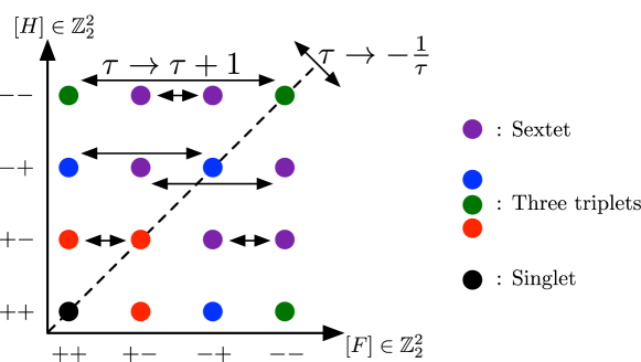
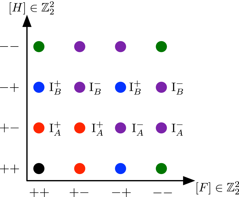
With the twisted homology groups (10) in hand, we can now classify the possible orientifolds of del Pezzo singularities with the geometric involution considered in §2.1. For dPk𝑑subscript𝑃𝑘dP_{k}, these are classified by [F],[H]H3(X5,~)2k+1delimited-[]𝐹delimited-[]𝐻superscript𝐻3subscript𝑋5~superscriptsubscript2𝑘1[F],[H]\in H^{3}(X_{5},\tilde{\mathbb{Z}})\cong\mathbb{Z}_{2}^{k+1}, for a total of 22k+2superscript22𝑘22^{2k+2} choices of discrete torsion. We divide these into five classes with ([F],[H])=(1,1)delimited-[]𝐹delimited-[]𝐻11([F],[H])=(1,1), ([F],[H])=(α,1)delimited-[]𝐹delimited-[]𝐻𝛼1([F],[H])=(\alpha,1), ([F],[H])=(1,α)delimited-[]𝐹delimited-[]𝐻1𝛼([F],[H])=(1,\alpha), ([F],[H])=(α,α)delimited-[]𝐹delimited-[]𝐻𝛼𝛼([F],[H])=(\alpha,\alpha), and ([F],[H])=(α,β)delimited-[]𝐹delimited-[]𝐻𝛼𝛽([F],[H])=(\alpha,\beta), where α𝛼\alpha and β𝛽\beta are distinct non-trivial elements of 2k+1superscriptsubscript2𝑘1\mathbb{Z}_{2}^{k+1}. The first class has a single member, the lone SL(2,)𝑆𝐿2SL(2,\mathbb{Z}) singlet. The second, third, and fourth classes each have 2k+11superscript2𝑘112^{k+1}-1 members, which together form 2k+11superscript2𝑘112^{k+1}-1 SL(2,)𝑆𝐿2SL(2,\mathbb{Z}) triplets, with orbits of the form (α,1),(1,α),(α,α)𝛼11𝛼𝛼𝛼(\alpha,1),(1,\alpha),(\alpha,\alpha). The last class has 2(2k+11)(2k1)2superscript2𝑘11superscript2𝑘12(2^{k+1}-1)(2^{k}-1) members, which form (2k+11)(2k1)3superscript2𝑘11superscript2𝑘13\frac{(2^{k+1}-1)(2^{k}-1)}{3} SL(2,)𝑆𝐿2SL(2,\mathbb{Z}) sextets, with orbits of the form (α,β),(β,α),(γ,β),(β,γ),(γ,α),(α,γ)𝛼𝛽𝛽𝛼𝛾𝛽𝛽𝛾𝛾𝛼𝛼𝛾(\alpha,\beta),(\beta,\alpha),(\gamma,\beta),(\beta,\gamma),(\gamma,\alpha),(\alpha,\gamma) where γ=αβ𝛾𝛼𝛽\gamma=\alpha\beta. The SL(2,)𝑆𝐿2SL(2,\mathbb{Z}) orbits of the various multiplets are illustrated in figure 9 for the case of dP1𝑑subscript𝑃1dP_{1}.

Refer to caption
Figure 9: Choices of discrete torsion for the dP1𝑑subscript𝑃1dP_{1} orientifold considered in the text. The 16 torsions arrange themselves into five irreducible representations — one singlet, three triplets, and one sextet — under the SL(2,)𝑆𝐿2SL(2,\mathbb{Z}) symmetry of type IIB string theory. The generator ττ+1𝜏𝜏1\tau\to\tau+1 maps the gs0subscript𝑔𝑠0g_{s}\to 0 cusps to themselves, hence the torsions connected by horizontal arrows correspond to the same cusp at different values of axion C0=Reτsubscript𝐶0Re𝜏C_{0}=\operatorname{Re}\tau.

Not all of the 22k+2superscript22𝑘22^{2k+2} choices of discrete torsion will lead to distinct gs0subscript𝑔𝑠0g_{s}\to 0 limits of the string theory background. Torsions related by [F][F]+[H]delimited-[]𝐹delimited-[]𝐹delimited-[]𝐻[F]\to[F]+[H] differ by a shift of the type IIB axion ττ+1𝜏𝜏1\tau\to\tau+1, and correspond to the same “cusp” on the modular curve parameterized by τ𝜏\tau. The number of distinct cusps depends on the SL(2,)𝑆𝐿2SL(2,\mathbb{Z}) multiplet: for singlets, there is only one, whereas for triplets there are two, and for sextets there are three. Adding up the results of the previous paragraph, we expect 2k(2k+1+1)superscript2𝑘superscript2𝑘112^{k}(2^{k+1}+1) cusps for the dPk𝑑subscript𝑃𝑘dP_{k} orientifold.

As in the well-understood 𝒩=4𝒩4\mathcal{N}=4 and orbifold cases dualities1 ; dualities2 , we expect each cusp to correspond to a distinct 𝒩=1𝒩1\mathcal{N}=1 gauge theory, some of which are related by S-duality. However, as shown in table 1, the number of cusps grows rapidly with k𝑘k, whereas the number of known field theory duals is extremely limited, as discussed in §2.2. For dP0𝑑subscript𝑃0dP_{0}, the gauge theory duals are in precise agreement with the discrete torsion classification dualities1 ; dualities2 . Conversely, for dPk𝑑subscript𝑃𝑘dP_{k}, k>1𝑘1k>1, no CFT duals are known, despite the large and rapidly growing number of cusps! Moreover, for dP1𝑑subscript𝑃1dP_{1}, only four distinct theories are known, two of which are S-dual, despite the expectation of five different SL(2,)𝑆𝐿2SL(2,\mathbb{Z}) orbits and ten different cusps!141414The situation for 𝔽0subscript𝔽0\mathbb{F}_{0} is similar, except that we need to account for the 2subscript2\mathbb{Z}_{2} discrete symmetry which exchanges the two 1superscript1\mathbb{P}^{1} factors and likewise the two generators of the twisted homology group H3(S3×S24,~)22superscript𝐻3superscript𝑆3superscript𝑆2subscript4~superscriptsubscript22H^{3}(\frac{S^{3}\times S^{2}}{\mathbb{Z}_{4}},\tilde{\mathbb{Z}})\cong\mathbb{Z}_{2}^{2}. Up to 2subscript2\mathbb{Z}_{2}-induced isomorphisms, we expect four different SL(2,)𝑆𝐿2SL(2,\mathbb{Z}) multiplets and seven different cusps, in contrast to the six known gauge theories, which occupy four different universality classes, two of which are S-dual dualities1 .

Singlets Triplets Sextets SL(2,)𝑆𝐿2SL(2,\mathbb{Z}) multiplets Cusps
dP0𝑑subscript𝑃0dP_{0} 1 1 0 2 3
dP1,𝔽0𝑑subscript𝑃1subscript𝔽0dP_{1},\mathbb{F}_{0} 1 3 1 5 10
dP2𝑑subscript𝑃2dP_{2} 1 7 7 15 36
dP3𝑑subscript𝑃3dP_{3} 1 15 35 51 136
dP4𝑑subscript𝑃4dP_{4} 1 31 155 187 528
dP5𝑑subscript𝑃5dP_{5} 1 63 651 715 2080
dP6𝑑subscript𝑃6dP_{6} 1 127 2667 2795 8256
dP7𝑑subscript𝑃7dP_{7} 1 255 10795 11051 32896
dP8𝑑subscript𝑃8dP_{8} 1 511 43435 43947 131328
Table 1: The discrete torsion classification of orientifolds of del Pezzo singularities. The 𝔽0subscript𝔽0\mathbb{F}_{0} singularity and many of the dPk𝑑subscript𝑃𝑘dP_{k}, k>1𝑘1k>1 singularities have discrete symmetries which relate a priori distinct choices of discrete torsion. The number of non-isomorphic cusps is smaller than shown here in these cases, but still very large.

There are three ways in which this paradox might be resolved. Either (i) the discrete torsion classification is incorrect, (ii) there are additional gauge theory duals which have not been found yet, or (iii) the missing cusps are not describable via perturbative gauge theories. In the remainder of this paper, we argue through a careful analysis of the dP1𝑑subscript𝑃1dP_{1} singularity that the latter possibility is the correct one. Fortunately, using a deconfinement-like trick we will nonetheless be able to construct perturbative gauge theories in the same universality class as the theories at the cusps, allowing us to describe some of their most important properties.

3 Phases of the dP1𝑑subscript𝑃1dP_{1} orientifold

We now specialize to the dP1𝑑subscript𝑃1dP_{1} orientifold described in §2. For reference, we reproduce the GLSM for the dP1𝑑subscript𝑃1dP_{1} singularity (1) below

z1z2z3z4tU(1)a10113U(1)b01012missing-subexpressionsubscript𝑧1subscript𝑧2subscript𝑧3subscript𝑧4𝑡missing-subexpressionmissing-subexpressionmissing-subexpressionmissing-subexpressionmissing-subexpressionmissing-subexpression𝑈subscript1𝑎10113𝑈subscript1𝑏01012\begin{array}[]{c|ccccc}&z_{1}&z_{2}&z_{3}&z_{4}&t\\ \hline\cr U(1)_{a}&1&0&1&1&-3\\ U(1)_{b}&0&1&0&1&-2\end{array} (12)

subject to the D-term conditions (2):

|z1|2+|z3|2+|z4|23|t|2=ξa,|z2|2+|z4|22|t|2=ξb,|z_{1}|^{2}+|z_{3}|^{2}+|z_{4}|^{2}-3|t|^{2}=\xi_{a}\qquad,\qquad|z_{2}|^{2}+|z_{4}|^{2}-2|t|^{2}=\xi_{b}\;, (13)

The toric diagram and web diagram for this singularity are shown in figure 10. The Fayet-Iliopoulos (FI) parameters ξasubscript𝜉𝑎\xi_{a} and ξbsubscript𝜉𝑏\xi_{b} control the resolutions of the singularity, as illustrated in figure 10(c), where the unresolved (affine) singularity corresponds to ξa=32ξb0subscript𝜉𝑎32subscript𝜉𝑏0\xi_{a}=\frac{3}{2}\xi_{b}\leq 0.

Refer to caption
(a) Toric diagram.
Refer to caption
(b) Dual web diagram.
Refer to caption
(c) Partial resolutions.
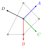
Figure 10: 10(a) Toric diagram associated to the complex cone over dP1𝑑subscript𝑃1dP_{1}. The labels refer to the corresponding fields in the GLSM (12). 10(b) The dual web diagram (or (p,q)𝑝𝑞(p,q) diagram) for the singular geometry. The external legs are labeled and colored for future reference. 10(c) Partial resolutions of the dP1𝑑subscript𝑃1dP_{1} singularity are controlled by the FI parameters ξasubscript𝜉𝑎\xi_{a} and ξbsubscript𝜉𝑏\xi_{b}.

We consider the orientifold involution tt𝑡𝑡t\to-t, as in §2.1. Blowing up in the region ξa>ξb>0subscript𝜉𝑎subscript𝜉𝑏0\xi_{a}>\xi_{b}>0, the exceptional divisor t=0𝑡0t=0 is dP1𝑑subscript𝑃1dP_{1}, which is wrapped by an O7 plane. Moving to the region ξb>ξa>0subscript𝜉𝑏subscript𝜉𝑎0\xi_{b}>\xi_{a}>0, the exceptional divisor develops a conifold singularity (at ξa=ξbsubscript𝜉𝑎subscript𝜉𝑏\xi_{a}=\xi_{b}) which flops, changing the topology of the divisor to dP0𝑑subscript𝑃0dP_{0}, still wrapped by an O7 plane. In the process, an O3 plane at z1=z2=z3=0subscript𝑧1subscript𝑧2subscript𝑧30z_{1}=z_{2}=z_{3}=0 splits off. Continuing into the region ξa<32ξbsubscript𝜉𝑎32subscript𝜉𝑏\xi_{a}<\frac{3}{2}\xi_{b}, ξa0subscript𝜉𝑎0\xi_{a}\leq 0, the O7 plane collapses into a 3/3superscript3subscript3\mathbb{C}^{3}/\mathbb{Z}_{3} orientifold singularity, leaving behind the O3 plane. In this region, the dP1𝑑subscript𝑃1dP_{1} singularity has split into two orbifold singularities, and the 22superscriptsubscript22\mathbb{Z}_{2}^{2} twisted homology group of the parent singularity maps on to the 2subscript2\mathbb{Z}_{2} twisted homology groups of the two components. Performing this partial resolution in the dual gauge theory and comparing with the known discrete torsions of orbifolds Witten:1998xy ; dualities1 ; dualities2 , we can read off the discrete torsion of the parent singularity.

3.1 Discrete torsion for the classical phases

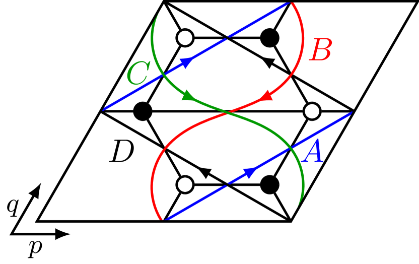
We apply this approach to the orientifolds IAsubscriptI𝐴\mathrm{I}_{A} and IBsubscriptI𝐵\mathrm{I}_{B} discussed in §2.2. For future reference, we reproduce the charge tables for phases IAsubscriptI𝐴\mathrm{I}_{A} and IBsubscriptI𝐵\mathrm{I}_{B} dualities1 in tables 2, 3. To read off the effect of the partial resolution to a 3/3superscript3subscript3\mathbb{C}^{3}/\mathbb{Z}_{3} orientifold singularity plus an O3 plane, as in the upper-left quadrant of figure 10(c), we need to identify which fields get a vev. As illustrated in figure 11, this can be done systematically by analyzing the zig-zag paths kenyonintro ; Hanany:2005ss ; Feng:2005gw of the dimer model, see GarciaEtxebarria:2006aq . Giving a vev to the fields where the zig-zag paths B𝐵B and C𝐶C cross combines the corresponding legs of the web diagram, which yields the web diagram for 3/3superscript3subscript3\mathbb{C}^{3}/\mathbb{Z}_{3}, hence the baryon in question corresponds to partial resolution to the 3/3superscript3subscript3\mathbb{C}^{3}/\mathbb{Z}_{3} orientifold singularity, as in the upper-left quadrant of figure 10(c), where the D3 branes remain on top of the singularity.

SU(N4)SU(N)SU(2)U(1)BU(1)YU(1)RAi ¯ 12N32(N4)1+2N42N4+2NY¯ ¯ 𝟏12N+32(N4)12N41+2N4+2NZ¯ 𝟏𝟏3N414N41+4N4Bi𝟏 1N014NX𝟏 𝟏1N114Nmissing-subexpression𝑆𝑈𝑁4𝑆𝑈𝑁𝑆𝑈2𝑈subscript1𝐵𝑈subscript1𝑌𝑈subscript1𝑅missing-subexpressionmissing-subexpressionmissing-subexpressionmissing-subexpressionmissing-subexpressionmissing-subexpressionmissing-subexpressionmissing-subexpressionmissing-subexpressionsuperscript𝐴𝑖 ¯absent 12𝑁32𝑁412𝑁42𝑁42𝑁missing-subexpression𝑌¯absent ¯absent 112𝑁32𝑁412𝑁412𝑁42𝑁missing-subexpression𝑍¯absent 113𝑁414𝑁414𝑁4missing-subexpressionsuperscript𝐵𝑖1 1𝑁014𝑁missing-subexpression𝑋1 11𝑁114𝑁missing-subexpression\begin{array}[]{c|cc|ccccc}&SU(N-4)&SU(N)&SU(2)&U(1)_{B}&U(1)_{Y}&U(1)_{R}\\ \hline\cr A^{i}&\leavevmode\hbox{$\vbox{\hbox{\vtop{ \offinterlineskip\openup-0.39993pt\halign{&\opttoksa@YT={\font@YT}\getcolor@YT{\save@YT{\opttoksb@YT}}\nil@YT\getcolor@YT{\startbox@@YT\the\opttoksa@YT\the\opttoksb@YT}#\endbox@YT\cr\lower 0.39993pt\vbox{\kern 0.19997pt\hbox{\kern 0.39993pt\vbox to5.39993pt{\vss\hbox to5.0pt{\hss$$\hss}\vss}\kern-5.39993pt\vrule height=5.39993pt,width=0.39993pt\kern 5.0pt\vrule height=5.39993pt,width=0.39993pt}\kern-0.19997pt\kern-5.39993pt\hrule width=5.79987pt,height=0.39993pt\kern 5.0pt\hrule width=5.79987pt,height=0.39993pt}\cr}}\kern 6.19986pt}}$}&\overline{}\leavevmode\hbox{$\vbox{\hbox{\vtop{ \offinterlineskip\openup-0.39993pt\halign{&\opttoksa@YT={\font@YT}\getcolor@YT{\save@YT{\opttoksb@YT}}\nil@YT\getcolor@YT{\startbox@@YT\the\opttoksa@YT\the\opttoksb@YT}#\endbox@YT\cr\lower 0.39993pt\vbox{\kern 0.19997pt\hbox{\kern 0.39993pt\vbox to5.39993pt{\vss\hbox to5.0pt{\hss$$\hss}\vss}\kern-5.39993pt\vrule height=5.39993pt,width=0.39993pt\kern 5.0pt\vrule height=5.39993pt,width=0.39993pt}\kern-0.19997pt\kern-5.39993pt\hrule width=5.79987pt,height=0.39993pt\kern 5.0pt\hrule width=5.79987pt,height=0.39993pt}\cr}}\kern 6.19986pt}}$}&\leavevmode\hbox{$\vbox{\hbox{\vtop{ \offinterlineskip\openup-0.39993pt\halign{&\opttoksa@YT={\font@YT}\getcolor@YT{\save@YT{\opttoksb@YT}}\nil@YT\getcolor@YT{\startbox@@YT\the\opttoksa@YT\the\opttoksb@YT}#\endbox@YT\cr\lower 0.39993pt\vbox{\kern 0.19997pt\hbox{\kern 0.39993pt\vbox to5.39993pt{\vss\hbox to5.0pt{\hss$$\hss}\vss}\kern-5.39993pt\vrule height=5.39993pt,width=0.39993pt\kern 5.0pt\vrule height=5.39993pt,width=0.39993pt}\kern-0.19997pt\kern-5.39993pt\hrule width=5.79987pt,height=0.39993pt\kern 5.0pt\hrule width=5.79987pt,height=0.39993pt}\cr}}\kern 6.19986pt}}$}&-\frac{1}{2N}-\frac{3}{2(N-4)}&1+\frac{2}{N-4}&-\frac{2}{N-4}+\frac{2}{N}\\ Y&\overline{}\leavevmode\hbox{$\vbox{\hbox{\vtop{ \offinterlineskip\openup-0.39993pt\halign{&\opttoksa@YT={\font@YT}\getcolor@YT{\save@YT{\opttoksb@YT}}\nil@YT\getcolor@YT{\startbox@@YT\the\opttoksa@YT\the\opttoksb@YT}#\endbox@YT\cr\lower 0.39993pt\vbox{\kern 0.19997pt\hbox{\kern 0.39993pt\vbox to5.39993pt{\vss\hbox to5.0pt{\hss$$\hss}\vss}\kern-5.39993pt\vrule height=5.39993pt,width=0.39993pt\kern 5.0pt\vrule height=5.39993pt,width=0.39993pt}\kern-0.19997pt\kern-5.39993pt\hrule width=5.79987pt,height=0.39993pt\kern 5.0pt\hrule width=5.79987pt,height=0.39993pt}\cr}}\kern 6.19986pt}}$}&\overline{}\leavevmode\hbox{$\vbox{\hbox{\vtop{ \offinterlineskip\openup-0.39993pt\halign{&\opttoksa@YT={\font@YT}\getcolor@YT{\save@YT{\opttoksb@YT}}\nil@YT\getcolor@YT{\startbox@@YT\the\opttoksa@YT\the\opttoksb@YT}#\endbox@YT\cr\lower 0.39993pt\vbox{\kern 0.19997pt\hbox{\kern 0.39993pt\vbox to5.39993pt{\vss\hbox to5.0pt{\hss$$\hss}\vss}\kern-5.39993pt\vrule height=5.39993pt,width=0.39993pt\kern 5.0pt\vrule height=5.39993pt,width=0.39993pt}\kern-0.19997pt\kern-5.39993pt\hrule width=5.79987pt,height=0.39993pt\kern 5.0pt\hrule width=5.79987pt,height=0.39993pt}\cr}}\kern 6.19986pt}}$}&{\bf 1}&-\frac{1}{2N}+\frac{3}{2(N-4)}&-1-\frac{2}{N-4}&1+\frac{2}{N-4}+\frac{2}{N}\\ Z&\overline{}\leavevmode\hbox{$\vbox{\hbox{\vtop{ \offinterlineskip\openup-0.39993pt\halign{&\opttoksa@YT={\font@YT}\getcolor@YT{\save@YT{\opttoksb@YT}}\nil@YT\getcolor@YT{\startbox@@YT\the\opttoksa@YT\the\opttoksb@YT}#\endbox@YT\cr\lower 0.39993pt\vbox{\kern 0.19997pt\hbox{\kern 0.39993pt\vbox to5.39993pt{\vss\hbox to5.0pt{\hss$$\hss}\vss}\kern-5.39993pt\vrule height=5.39993pt,width=0.39993pt\kern 5.0pt\vrule height=5.39993pt,width=0.39993pt}\kern-0.19997pt\kern-5.39993pt\hrule width=5.79987pt,height=0.39993pt\kern 5.0pt\hrule width=5.79987pt,height=0.39993pt}&\lower 0.39993pt\vbox{\kern 0.19997pt\hbox{\kern 0.39993pt\vbox to5.39993pt{\vss\hbox to5.0pt{\hss$$\hss}\vss}\kern-5.39993pt\vrule height=5.39993pt,width=0.39993pt\kern 5.0pt\vrule height=5.39993pt,width=0.39993pt}\kern-0.19997pt\kern-5.39993pt\hrule width=5.79987pt,height=0.39993pt\kern 5.0pt\hrule width=5.79987pt,height=0.39993pt}\cr}}\kern 11.99973pt}}$}&{\bf 1}&{\bf 1}&\frac{3}{N-4}&-1-\frac{4}{N-4}&1+\frac{4}{N-4}\\ B^{i}&{\bf 1}&\leavevmode\hbox{$\vbox{\hbox{\vtop{ \offinterlineskip\openup-0.39993pt\halign{&\opttoksa@YT={\font@YT}\getcolor@YT{\save@YT{\opttoksb@YT}}\nil@YT\getcolor@YT{\startbox@@YT\the\opttoksa@YT\the\opttoksb@YT}#\endbox@YT\cr\lower 0.39993pt\vbox{\kern 0.19997pt\hbox{\kern 0.39993pt\vbox to5.39993pt{\vss\hbox to5.0pt{\hss$$\hss}\vss}\kern-5.39993pt\vrule height=5.39993pt,width=0.39993pt\kern 5.0pt\vrule height=5.39993pt,width=0.39993pt}\kern-0.19997pt\kern-5.39993pt\hrule width=5.79987pt,height=0.39993pt\kern 5.0pt\hrule width=5.79987pt,height=0.39993pt}\cr\lower 0.39993pt\vbox{\kern 0.19997pt\hbox{\kern 0.39993pt\vbox to5.39993pt{\vss\hbox to5.0pt{\hss$$\hss}\vss}\kern-5.39993pt\vrule height=5.39993pt,width=0.39993pt\kern 5.0pt\vrule height=5.39993pt,width=0.39993pt}\kern-0.19997pt\kern-5.39993pt\hrule width=5.79987pt,height=0.39993pt\kern 5.0pt\hrule width=5.79987pt,height=0.39993pt}\cr}}\kern 6.19986pt}}$}&\leavevmode\hbox{$\vbox{\hbox{\vtop{ \offinterlineskip\openup-0.39993pt\halign{&\opttoksa@YT={\font@YT}\getcolor@YT{\save@YT{\opttoksb@YT}}\nil@YT\getcolor@YT{\startbox@@YT\the\opttoksa@YT\the\opttoksb@YT}#\endbox@YT\cr\lower 0.39993pt\vbox{\kern 0.19997pt\hbox{\kern 0.39993pt\vbox to5.39993pt{\vss\hbox to5.0pt{\hss$$\hss}\vss}\kern-5.39993pt\vrule height=5.39993pt,width=0.39993pt\kern 5.0pt\vrule height=5.39993pt,width=0.39993pt}\kern-0.19997pt\kern-5.39993pt\hrule width=5.79987pt,height=0.39993pt\kern 5.0pt\hrule width=5.79987pt,height=0.39993pt}\cr}}\kern 6.19986pt}}$}&\frac{1}{N}&0&1-\frac{4}{N}\\ X&{\bf 1}&\leavevmode\hbox{$\vbox{\hbox{\vtop{ \offinterlineskip\openup-0.39993pt\halign{&\opttoksa@YT={\font@YT}\getcolor@YT{\save@YT{\opttoksb@YT}}\nil@YT\getcolor@YT{\startbox@@YT\the\opttoksa@YT\the\opttoksb@YT}#\endbox@YT\cr\lower 0.39993pt\vbox{\kern 0.19997pt\hbox{\kern 0.39993pt\vbox to5.39993pt{\vss\hbox to5.0pt{\hss$$\hss}\vss}\kern-5.39993pt\vrule height=5.39993pt,width=0.39993pt\kern 5.0pt\vrule height=5.39993pt,width=0.39993pt}\kern-0.19997pt\kern-5.39993pt\hrule width=5.79987pt,height=0.39993pt\kern 5.0pt\hrule width=5.79987pt,height=0.39993pt}\cr\lower 0.39993pt\vbox{\kern 0.19997pt\hbox{\kern 0.39993pt\vbox to5.39993pt{\vss\hbox to5.0pt{\hss$$\hss}\vss}\kern-5.39993pt\vrule height=5.39993pt,width=0.39993pt\kern 5.0pt\vrule height=5.39993pt,width=0.39993pt}\kern-0.19997pt\kern-5.39993pt\hrule width=5.79987pt,height=0.39993pt\kern 5.0pt\hrule width=5.79987pt,height=0.39993pt}\cr}}\kern 6.19986pt}}$}&{\bf 1}&\frac{1}{N}&-1&1-\frac{4}{N}\end{array}
Table 2: Phase IAsubscriptI𝐴\mathrm{I}_{A}
SU(N~+4)SU(N~)SU(2)U(1)BU(1)YU(1)RA~i ¯ 12N~32(N~+4)12N~+42N~+42N~Y~¯ ¯ 𝟏12N~+32(N~+4)1+2N~+412N~+42N~Z~¯ 𝟏𝟏3N~+41+4N~+414N~+4B~i𝟏 1N~01+4N~X~𝟏 𝟏1N~11+4N~missing-subexpression𝑆𝑈~𝑁4𝑆𝑈~𝑁𝑆𝑈2𝑈subscript1𝐵𝑈subscript1𝑌𝑈subscript1𝑅missing-subexpressionmissing-subexpressionmissing-subexpressionmissing-subexpressionmissing-subexpressionmissing-subexpressionmissing-subexpressionmissing-subexpressionmissing-subexpressionsuperscript~𝐴𝑖 ¯absent 12~𝑁32~𝑁412~𝑁42~𝑁42~𝑁missing-subexpression~𝑌¯absent ¯absent 112~𝑁32~𝑁412~𝑁412~𝑁42~𝑁missing-subexpression~𝑍¯absent 113~𝑁414~𝑁414~𝑁4missing-subexpressionsuperscript~𝐵𝑖1 1~𝑁014~𝑁missing-subexpression~𝑋1 11~𝑁114~𝑁missing-subexpression\begin{array}[]{c|cc|ccccc}&SU({\widetilde{N}}+4)&SU({\widetilde{N}})&SU(2)&U(1)_{B}&U(1)_{Y}&U(1)_{R}\\ \hline\cr\tilde{A}^{i}&\leavevmode\hbox{$\vbox{\hbox{\vtop{ \offinterlineskip\openup-0.39993pt\halign{&\opttoksa@YT={\font@YT}\getcolor@YT{\save@YT{\opttoksb@YT}}\nil@YT\getcolor@YT{\startbox@@YT\the\opttoksa@YT\the\opttoksb@YT}#\endbox@YT\cr\lower 0.39993pt\vbox{\kern 0.19997pt\hbox{\kern 0.39993pt\vbox to5.39993pt{\vss\hbox to5.0pt{\hss$$\hss}\vss}\kern-5.39993pt\vrule height=5.39993pt,width=0.39993pt\kern 5.0pt\vrule height=5.39993pt,width=0.39993pt}\kern-0.19997pt\kern-5.39993pt\hrule width=5.79987pt,height=0.39993pt\kern 5.0pt\hrule width=5.79987pt,height=0.39993pt}\cr}}\kern 6.19986pt}}$}&\overline{}\leavevmode\hbox{$\vbox{\hbox{\vtop{ \offinterlineskip\openup-0.39993pt\halign{&\opttoksa@YT={\font@YT}\getcolor@YT{\save@YT{\opttoksb@YT}}\nil@YT\getcolor@YT{\startbox@@YT\the\opttoksa@YT\the\opttoksb@YT}#\endbox@YT\cr\lower 0.39993pt\vbox{\kern 0.19997pt\hbox{\kern 0.39993pt\vbox to5.39993pt{\vss\hbox to5.0pt{\hss$$\hss}\vss}\kern-5.39993pt\vrule height=5.39993pt,width=0.39993pt\kern 5.0pt\vrule height=5.39993pt,width=0.39993pt}\kern-0.19997pt\kern-5.39993pt\hrule width=5.79987pt,height=0.39993pt\kern 5.0pt\hrule width=5.79987pt,height=0.39993pt}\cr}}\kern 6.19986pt}}$}&\leavevmode\hbox{$\vbox{\hbox{\vtop{ \offinterlineskip\openup-0.39993pt\halign{&\opttoksa@YT={\font@YT}\getcolor@YT{\save@YT{\opttoksb@YT}}\nil@YT\getcolor@YT{\startbox@@YT\the\opttoksa@YT\the\opttoksb@YT}#\endbox@YT\cr\lower 0.39993pt\vbox{\kern 0.19997pt\hbox{\kern 0.39993pt\vbox to5.39993pt{\vss\hbox to5.0pt{\hss$$\hss}\vss}\kern-5.39993pt\vrule height=5.39993pt,width=0.39993pt\kern 5.0pt\vrule height=5.39993pt,width=0.39993pt}\kern-0.19997pt\kern-5.39993pt\hrule width=5.79987pt,height=0.39993pt\kern 5.0pt\hrule width=5.79987pt,height=0.39993pt}\cr}}\kern 6.19986pt}}$}&-\frac{1}{2{\widetilde{N}}}-\frac{3}{2({\widetilde{N}}+4)}&1-\frac{2}{{\widetilde{N}}+4}&\frac{2}{{\widetilde{N}}+4}-\frac{2}{{\widetilde{N}}}\\ \tilde{Y}&\overline{}\leavevmode\hbox{$\vbox{\hbox{\vtop{ \offinterlineskip\openup-0.39993pt\halign{&\opttoksa@YT={\font@YT}\getcolor@YT{\save@YT{\opttoksb@YT}}\nil@YT\getcolor@YT{\startbox@@YT\the\opttoksa@YT\the\opttoksb@YT}#\endbox@YT\cr\lower 0.39993pt\vbox{\kern 0.19997pt\hbox{\kern 0.39993pt\vbox to5.39993pt{\vss\hbox to5.0pt{\hss$$\hss}\vss}\kern-5.39993pt\vrule height=5.39993pt,width=0.39993pt\kern 5.0pt\vrule height=5.39993pt,width=0.39993pt}\kern-0.19997pt\kern-5.39993pt\hrule width=5.79987pt,height=0.39993pt\kern 5.0pt\hrule width=5.79987pt,height=0.39993pt}\cr}}\kern 6.19986pt}}$}&\overline{}\leavevmode\hbox{$\vbox{\hbox{\vtop{ \offinterlineskip\openup-0.39993pt\halign{&\opttoksa@YT={\font@YT}\getcolor@YT{\save@YT{\opttoksb@YT}}\nil@YT\getcolor@YT{\startbox@@YT\the\opttoksa@YT\the\opttoksb@YT}#\endbox@YT\cr\lower 0.39993pt\vbox{\kern 0.19997pt\hbox{\kern 0.39993pt\vbox to5.39993pt{\vss\hbox to5.0pt{\hss$$\hss}\vss}\kern-5.39993pt\vrule height=5.39993pt,width=0.39993pt\kern 5.0pt\vrule height=5.39993pt,width=0.39993pt}\kern-0.19997pt\kern-5.39993pt\hrule width=5.79987pt,height=0.39993pt\kern 5.0pt\hrule width=5.79987pt,height=0.39993pt}\cr}}\kern 6.19986pt}}$}&{\bf 1}&-\frac{1}{2{\widetilde{N}}}+\frac{3}{2({\widetilde{N}}+4)}&-1+\frac{2}{{\widetilde{N}}+4}&1-\frac{2}{{\widetilde{N}}+4}-\frac{2}{{\widetilde{N}}}\\ \tilde{Z}&\overline{}\leavevmode\hbox{$\vbox{\hbox{\vtop{ \offinterlineskip\openup-0.39993pt\halign{&\opttoksa@YT={\font@YT}\getcolor@YT{\save@YT{\opttoksb@YT}}\nil@YT\getcolor@YT{\startbox@@YT\the\opttoksa@YT\the\opttoksb@YT}#\endbox@YT\cr\lower 0.39993pt\vbox{\kern 0.19997pt\hbox{\kern 0.39993pt\vbox to5.39993pt{\vss\hbox to5.0pt{\hss$$\hss}\vss}\kern-5.39993pt\vrule height=5.39993pt,width=0.39993pt\kern 5.0pt\vrule height=5.39993pt,width=0.39993pt}\kern-0.19997pt\kern-5.39993pt\hrule width=5.79987pt,height=0.39993pt\kern 5.0pt\hrule width=5.79987pt,height=0.39993pt}\cr\lower 0.39993pt\vbox{\kern 0.19997pt\hbox{\kern 0.39993pt\vbox to5.39993pt{\vss\hbox to5.0pt{\hss$$\hss}\vss}\kern-5.39993pt\vrule height=5.39993pt,width=0.39993pt\kern 5.0pt\vrule height=5.39993pt,width=0.39993pt}\kern-0.19997pt\kern-5.39993pt\hrule width=5.79987pt,height=0.39993pt\kern 5.0pt\hrule width=5.79987pt,height=0.39993pt}\cr}}\kern 6.19986pt}}$}&{\bf 1}&{\bf 1}&\frac{3}{{\widetilde{N}}+4}&-1+\frac{4}{{\widetilde{N}}+4}&1-\frac{4}{{\widetilde{N}}+4}\\ \tilde{B}^{i}&{\bf 1}&\leavevmode\hbox{$\vbox{\hbox{\vtop{ \offinterlineskip\openup-0.39993pt\halign{&\opttoksa@YT={\font@YT}\getcolor@YT{\save@YT{\opttoksb@YT}}\nil@YT\getcolor@YT{\startbox@@YT\the\opttoksa@YT\the\opttoksb@YT}#\endbox@YT\cr\lower 0.39993pt\vbox{\kern 0.19997pt\hbox{\kern 0.39993pt\vbox to5.39993pt{\vss\hbox to5.0pt{\hss$$\hss}\vss}\kern-5.39993pt\vrule height=5.39993pt,width=0.39993pt\kern 5.0pt\vrule height=5.39993pt,width=0.39993pt}\kern-0.19997pt\kern-5.39993pt\hrule width=5.79987pt,height=0.39993pt\kern 5.0pt\hrule width=5.79987pt,height=0.39993pt}&\lower 0.39993pt\vbox{\kern 0.19997pt\hbox{\kern 0.39993pt\vbox to5.39993pt{\vss\hbox to5.0pt{\hss$$\hss}\vss}\kern-5.39993pt\vrule height=5.39993pt,width=0.39993pt\kern 5.0pt\vrule height=5.39993pt,width=0.39993pt}\kern-0.19997pt\kern-5.39993pt\hrule width=5.79987pt,height=0.39993pt\kern 5.0pt\hrule width=5.79987pt,height=0.39993pt}\cr}}\kern 11.99973pt}}$}&\leavevmode\hbox{$\vbox{\hbox{\vtop{ \offinterlineskip\openup-0.39993pt\halign{&\opttoksa@YT={\font@YT}\getcolor@YT{\save@YT{\opttoksb@YT}}\nil@YT\getcolor@YT{\startbox@@YT\the\opttoksa@YT\the\opttoksb@YT}#\endbox@YT\cr\lower 0.39993pt\vbox{\kern 0.19997pt\hbox{\kern 0.39993pt\vbox to5.39993pt{\vss\hbox to5.0pt{\hss$$\hss}\vss}\kern-5.39993pt\vrule height=5.39993pt,width=0.39993pt\kern 5.0pt\vrule height=5.39993pt,width=0.39993pt}\kern-0.19997pt\kern-5.39993pt\hrule width=5.79987pt,height=0.39993pt\kern 5.0pt\hrule width=5.79987pt,height=0.39993pt}\cr}}\kern 6.19986pt}}$}&\frac{1}{{\widetilde{N}}}&0&1+\frac{4}{{\widetilde{N}}}\\ \tilde{X}&{\bf 1}&\leavevmode\hbox{$\vbox{\hbox{\vtop{ \offinterlineskip\openup-0.39993pt\halign{&\opttoksa@YT={\font@YT}\getcolor@YT{\save@YT{\opttoksb@YT}}\nil@YT\getcolor@YT{\startbox@@YT\the\opttoksa@YT\the\opttoksb@YT}#\endbox@YT\cr\lower 0.39993pt\vbox{\kern 0.19997pt\hbox{\kern 0.39993pt\vbox to5.39993pt{\vss\hbox to5.0pt{\hss$$\hss}\vss}\kern-5.39993pt\vrule height=5.39993pt,width=0.39993pt\kern 5.0pt\vrule height=5.39993pt,width=0.39993pt}\kern-0.19997pt\kern-5.39993pt\hrule width=5.79987pt,height=0.39993pt\kern 5.0pt\hrule width=5.79987pt,height=0.39993pt}&\lower 0.39993pt\vbox{\kern 0.19997pt\hbox{\kern 0.39993pt\vbox to5.39993pt{\vss\hbox to5.0pt{\hss$$\hss}\vss}\kern-5.39993pt\vrule height=5.39993pt,width=0.39993pt\kern 5.0pt\vrule height=5.39993pt,width=0.39993pt}\kern-0.19997pt\kern-5.39993pt\hrule width=5.79987pt,height=0.39993pt\kern 5.0pt\hrule width=5.79987pt,height=0.39993pt}\cr}}\kern 11.99973pt}}$}&{\bf 1}&\frac{1}{{\widetilde{N}}}&-1&1+\frac{4}{{\widetilde{N}}}\end{array}
Table 3: Phase IBsubscriptI𝐵\mathrm{I}_{B}

There is another baryonic branch where the D3 branes are carried away on top of the O3 plane, corresponding to a vev for the fields where the zig-zag paths A𝐴A and D𝐷D cross. More generally, some number of D3 branes can remain on the 3/3superscript3subscript3\mathbb{C}^{3}/\mathbb{Z}_{3} orientifold singularity while the others are carried away on top of the O3 plane.151515There are, of course, other directions in moduli space where the D3 branes do not lie atop either of the resulting O-planes, but these directions are not relevant to the present discussion. The corresponding baryon – a mixture of the two described above – was identified in dualities1 :

𝒪p=ZN4p(XY2)p,𝒪~p~=Z~N~+4p~(X~Y~2)p~,formulae-sequencesubscript𝒪𝑝superscript𝑍𝑁4𝑝superscript𝑋superscript𝑌2𝑝subscript~𝒪~𝑝superscript~𝑍~𝑁4~𝑝superscript~𝑋superscript~𝑌2~𝑝\mathcal{O}_{p}=Z^{N-4-p}(XY^{2})^{p}\;\;,\;\;\widetilde{\mathcal{O}}_{\tilde{p}}=\tilde{Z}^{{\widetilde{N}}+4-\tilde{p}}(\tilde{X}\tilde{Y}^{2})^{\tilde{p}}\,, (14)

for IAsubscriptI𝐴\mathrm{I}_{A} and IBsubscriptI𝐵\mathrm{I}_{B}, respectively, where p𝑝p and N~p~~𝑁~𝑝{\widetilde{N}}-\tilde{p} must be even. Turning on a vev for 𝒪psubscript𝒪𝑝\mathcal{O}_{p} or 𝒪~p~subscript~𝒪~𝑝\widetilde{\mathcal{O}}_{\tilde{p}} breaks

𝒪p:SU(N4)×SU(N)[SO(N4p)×SU(Np)]×USp(p),𝒪~p~:SU(N~+4)×SU(N~)[USp(N~+4p~)×SU(N~p~)]×SO(p~).:subscript𝒪𝑝𝑆𝑈𝑁4𝑆𝑈𝑁delimited-[]𝑆𝑂𝑁4𝑝𝑆𝑈𝑁𝑝𝑈𝑆𝑝𝑝subscript~𝒪~𝑝:𝑆𝑈~𝑁4𝑆𝑈~𝑁delimited-[]𝑈𝑆𝑝~𝑁4~𝑝𝑆𝑈~𝑁~𝑝𝑆𝑂~𝑝\begin{split}\mathcal{O}_{p}:&\qquad SU(N-4)\times SU(N)\longrightarrow[SO(N-4-p)\times SU(N-p)]\times U\!Sp(p)\,,\\ \widetilde{\mathcal{O}}_{\tilde{p}}:&\qquad SU({\widetilde{N}}+4)\times SU({\widetilde{N}})\longrightarrow[U\!Sp({\widetilde{N}}+4-\tilde{p})\times SU({\widetilde{N}}-\tilde{p})]\times SO(\tilde{p})\,.\end{split} (15)

Keeping track of the chiral superfields which are Higgsed or which acquire a mass from the superpotential, we find that the USp(p)𝑈𝑆𝑝𝑝U\!Sp(p) and SO(p~)𝑆𝑂~𝑝SO(\tilde{p}) factors decouple from the rest of the gauge group, with an 𝒩=4𝒩4\mathcal{N}=4 spectrum and interactions, whereas the remaining fields and interactions reproduce those of the 3/3superscript3subscript3\mathbb{C}^{3}/\mathbb{Z}_{3} orientifold studied in dualities1 , as illustrated in figure 12(a).
Refer to caption
(a) Zig-zag paths.
Refer to caption
(b) Higgsing to 3/3superscript3subscript3\mathbb{C}^{3}/\mathbb{Z}_{3}.
Refer to caption
(c) Higgsing to 3superscript3\mathbb{C}^{3}.
Figure 11: 11(a) The zig-zag paths for the dP1𝑑subscript𝑃1dP_{1} dimer model, figure 4(a). The winding numbers of the zig-zag paths reproduce the directions of the homonymous legs in the web diagram, figure 10(b). 11(b) Partial resolution to 3/3superscript3subscript3\mathbb{C}^{3}/\mathbb{Z}_{3} corresponds to a vev for the fields where paths B𝐵B and C𝐶C cross. 11(c) Partial resolution to 3superscript3\mathbb{C}^{3} corresponds to a vev for the fields where paths A𝐴A and D𝐷D cross. An 𝒩=4𝒩4\mathcal{N}=4 theory is obtained upon integrating out the massive matter.
Refer to caption
(a) Partial resolution of IAsubscriptI𝐴\mathrm{I}_{A}.
Refer to caption
(b) Discrete torsion for IAsubscriptI𝐴\mathrm{I}_{A} and IBsubscriptI𝐵\mathrm{I}_{B}.
Figure 12: 12(a) Partial resolution of the dP1𝑑subscript𝑃1dP_{1} singularity as realized in phase IAsubscriptI𝐴\mathrm{I}_{A}. Phase IBsubscriptI𝐵\mathrm{I}_{B} is analogous. 12(b) Assignment of discrete torsions (in the basis associated to the partial resolution) to phases IAsubscriptI𝐴\mathrm{I}_{A} and IBsubscriptI𝐵\mathrm{I}_{B}.

We verify that this result is consistent with D3 charge conservation. The 𝒩=4𝒩4\mathcal{N}=4 theories (coming from D3 branes on top of an O3 plane in a smooth background) have D3 brane charge

Q3SO(p)=p12,Q3USp(p)=p+12,formulae-sequencesubscriptsuperscript𝑄𝑆𝑂𝑝superscript3𝑝12subscriptsuperscript𝑄𝑈𝑆𝑝𝑝superscript3𝑝12Q^{SO(p)}_{\mathbb{C}^{3}}=p-\frac{1}{2}\;\;,\;\;Q^{U\!Sp(p)}_{\mathbb{C}^{3}}=p+\frac{1}{2}\,, (16)

whereas the 3/3superscript3subscript3\mathbb{C}^{3}/\mathbb{Z}_{3} orientifold theories have D3 brane charge dualities2

Q3/3SO(p4)×SU(p)=p32,Q3/3USp(p+4)×SU(p)=p+32,formulae-sequencesubscriptsuperscript𝑄𝑆𝑂𝑝4𝑆𝑈𝑝superscript3subscript3𝑝32subscriptsuperscript𝑄𝑈𝑆𝑝𝑝4𝑆𝑈𝑝superscript3subscript3𝑝32Q^{SO(p-4)\times SU(p)}_{\mathbb{C}^{3}/\mathbb{Z}_{3}}=p-\frac{3}{2}\;\;,\;\;Q^{U\!Sp(p+4)\times SU(p)}_{\mathbb{C}^{3}/\mathbb{Z}_{3}}=p+\frac{3}{2}\,, (17)

where we measure the charge in the Calabi-Yau double cover, so that a mobile D3 brane has charge +22+2. Adding together the charges of the two components, we obtain the charge of the dP1𝑑subscript𝑃1dP_{1} orientifold singularity in each phase:

QIASU(N4)×SU(N)=N1,QIBSU(N~+4)×SU(N~)=N~+1.formulae-sequencesuperscriptsubscript𝑄subscriptI𝐴𝑆𝑈𝑁4𝑆𝑈𝑁𝑁1superscriptsubscript𝑄subscriptI𝐵𝑆𝑈~𝑁4𝑆𝑈~𝑁~𝑁1Q_{\mathrm{I}_{A}}^{SU(N-4)\times SU(N)}=N-1\;\;,\;\;Q_{\mathrm{I}_{B}}^{SU({\widetilde{N}}+4)\times SU({\widetilde{N}})}={\widetilde{N}}+1\,. (18)

This result can be verified using the explicit construction of the fractional branes given in appendix B.

The result (15) encodes the discrete torsion of the parent dP1𝑑subscript𝑃1dP_{1} orientifold singularity as follows. For the 𝒩=4𝒩4\mathcal{N}=4 theories as well as for the 3/3superscript3subscript3\mathbb{C}^{3}/\mathbb{Z}_{3} orientifold theories, the gauge groups with an SO(p)𝑆𝑂𝑝SO(p) factor have torsion [F]=()pdelimited-[]𝐹superscript𝑝[F]=(-)^{p} and [H]=+delimited-[]𝐻[H]=+ and those with an USp(p)𝑈𝑆𝑝𝑝U\!Sp(p) factor have torsion [F]=±delimited-[]𝐹plus-or-minus[F]=\pm and [H]=delimited-[]𝐻[H]=-, where in the latter case the two choices of [F]delimited-[]𝐹[F] correspond to the same cusp at different values of C0subscript𝐶0C_{0}. Thus, the discrete torsion of the IAsubscriptI𝐴\mathrm{I}_{A} theory is [F]=(()N,±)delimited-[]𝐹superscript𝑁plus-or-minus[F]=((-)^{N},\pm) and [H]=(+,)delimited-[]𝐻[H]=(+,-) in a basis where (,+)(-,+) generates the 2subscript2\mathbb{Z}_{2} associated to the 3/3superscript3subscript3\mathbb{C}^{3}/\mathbb{Z}_{3} singularity and (+,)(+,-) generates the 2subscript2\mathbb{Z}_{2} associated to the O3 plane. Likewise, the discrete torsion for the IBsubscriptI𝐵\mathrm{I}_{B} theory is [F]=(±,()N~)delimited-[]𝐹plus-or-minussuperscript~𝑁[F]=(\pm,(-)^{\widetilde{N}}) and [H]=(,+)delimited-[]𝐻[H]=(-,+) in the same basis.

Using this information we can start filling in some of the dots in figure 9. We denote by IA±superscriptsubscriptI𝐴plus-or-minus\mathrm{I}_{A}^{\pm} the IAsubscriptI𝐴\mathrm{I}_{A} theory with (1)N=±1superscript1𝑁plus-or-minus1(-1)^{N}=\pm 1, and similarly by IB±superscriptsubscriptI𝐵plus-or-minus\mathrm{I}_{B}^{\pm} the IBsubscriptI𝐵\mathrm{I}_{B} theory with (1)N~=±1superscript1~𝑁plus-or-minus1(-1)^{\widetilde{N}}=\pm 1. The result of the above argument is depicted in figure 12(b). Notice that IAsuperscriptsubscriptI𝐴\mathrm{I}_{A}^{-} and IBsuperscriptsubscriptI𝐵\mathrm{I}_{B}^{-} fall in the same SL(2,)𝑆𝐿2SL(2,\mathbb{Z}) multiplet, hence they should be S-duals. Conservation of D3 charge (18) requires N~=N2~𝑁𝑁2{\widetilde{N}}=N-2. This duality was already conjectured purely on the basis of field theory evidence in dualities1 , including a non-trivial matching between the low-N𝑁N dynamics. We provide further evidence for this duality in §5.1, where we match a large number of terms in the superconformal index, limited only by the running time of an optimized program. The discrete torsion assignment in figure 12 provides a much clearer picture of why this duality exists for odd N𝑁N and not for even N𝑁N. It also highlights the gaps in the first and last rows, including the S-duals of the even N𝑁N theories, whose absence was a mystery in dualities1 . In fact, none of the SL(2,)𝑆𝐿2SL(2,\mathbb{Z}) multiplets are complete, including the one containing the S-dual pair IAsuperscriptsubscriptI𝐴\mathrm{I}_{A}^{-} and IBsuperscriptsubscriptI𝐵\mathrm{I}_{B}^{-}.

3.2 Brane tilings and orientifolds

We now explain why these theories are absent, which is the first step along the way to constructing them.

While our main focus is dP1𝑑subscript𝑃1dP_{1}, we find it convenient in the present discussion to consider a generic isolated toric singularity with k+3𝑘3k+3 legs in the web diagram — for which there are k𝑘k two-cycles in the horizon Y5subscript𝑌5Y_{5} of the singularity, and for which the twisted homology group is 2k+1superscriptsubscript2𝑘1\mathbb{Z}_{2}^{k+1} toricII — for example dPk𝑑subscript𝑃𝑘dP_{k}, k=0,1,2,3𝑘0123k=0,1,2,3.

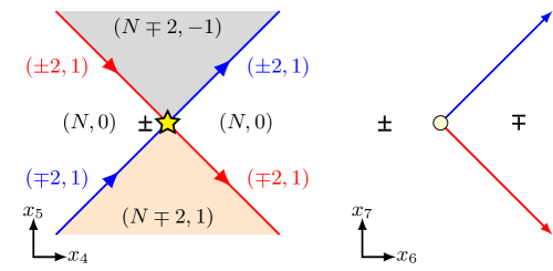
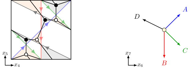
We first review the construction of dimer models from NS5-D5 systems, as discussed in e.g. Yamazaki:2008bt . Consider type IIB string theory on T2×4superscript𝑇2superscript4T^{2}\times\mathbb{R}^{4},161616All of the branes we consider wrap the directions x0,x3subscript𝑥0subscript𝑥3x_{0},\ldots x_{3}, and none wrap the directions x8,x9subscript𝑥8subscript𝑥9x_{8},x_{9}. with a flat background metric, where x4x4+1similar-tosubscript𝑥4subscript𝑥41x_{4}\sim x_{4}+1 and x5x5+1similar-tosubscript𝑥5subscript𝑥51x_{5}\sim x_{5}+1 parameterize the torus. We wrap N𝑁N D5 branes — the double T-dual of the N𝑁N D3 branes we started with — on the T2superscript𝑇2T^{2}. To reproduce the original Calabi-Yau geometry, we introduce NS5 branes ending on one-cycles of the torus and extending outwards along rays in the (x6,x7)subscript𝑥6subscript𝑥7(x_{6},x_{7}) directions. Specifically, for an NS5 brane ending on the (p,q)𝑝𝑞(p,q) cycle of the torus, the corresponding ray — (x6,x7)=(tp,tq)subscript𝑥6subscript𝑥7𝑡𝑝𝑡𝑞(x_{6},x_{7})=(tp,tq) with t[0,)𝑡0t\in[0,\infty) — is chosen to preserve a common 𝒩=1𝒩1\mathcal{N}=1 supersymmetry with the other NS5 branes and with the D5 branes. The cycles wrapped by the NS5 branes correspond to the legs of the web diagram of the toric singularity in question, see e.g. figure 10(b).

To satisfy five-brane charge conservation, the NS5 branes cannot simply end on the torus. Instead, they divide the torus into (N,Q)𝑁𝑄(N,Q) D5-NS5 bound states with different Q𝑄Q’s, where steps in Q𝑄Q across the NS5 brane cycles account for the tadpole induced by the boundary of the NS5 brane. To obtain a gauge theory description, we restrict to configurations with Q=0,±1𝑄0plus-or-minus1Q=0,\pm 1, where the (N,0)𝑁0(N,0) branes carry a U(N)𝑈𝑁U(N) gauge group, whereas (N,1)𝑁1(N,1) and (N,1)𝑁1(N,-1) carry only a U(1)𝑈1U(1) gauge group. In the low-energy limit, the U(1)𝑈1U(1)’s become massive or decouple, and we are left with a quiver gauge theory with the (N,0)𝑁0(N,0) faces as nodes. Wherever two NS5 branes intersect, two of the (N,0)𝑁0(N,0) faces touch each other, and there is bifundamental matter, which is chiral due to the presence of the NS5 branes. For each (N,1)𝑁1(N,1) and (N,1)𝑁1(N,-1) face, there is a corresponding disk diagram which generates a term in the superpotential out of the matter fields surrounding the face.

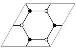
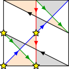
This construction is illustrated in figure 13 for dP1𝑑subscript𝑃1dP_{1}. We refer to the configuration of five branes along the torus as a “brane tiling”.171717Our usage here is somewhat more specific than is common in the literature. We have reserved the phrase “brane tiling” for a physical configuration of branes, in contrast to dimer models, which represent a broader class of quiver gauge theories. Dualizing the brane tiling, we recover the dimer model (figure 1(a)) for dP1𝑑subscript𝑃1dP_{1}, where the (N,0)𝑁0(N,0) branes map to faces, the (N,1)𝑁1(N,1) and (N,1)𝑁1(N,-1) branes to white and black nodes, respectively, and the NS5-brane intersections to edges. The NS5 branes correspond to zig-zag paths in the dimer model.
Refer to caption
Figure 13: The brane tiling corresponding to the dP1𝑑subscript𝑃1dP_{1} singularity and the dual dimer model, c.f. figure 11(a).

The above description of the NS5-D5 system is valid in the gssubscript𝑔𝑠g_{s}\to\infty limit, where the NS5 brane tension is much less than the D5 brane tension.181818See Yamazaki:2008bt for a precise definition of the gssubscript𝑔𝑠g_{s}\to\infty and gs0subscript𝑔𝑠0g_{s}\to 0 limits. In the gs0subscript𝑔𝑠0g_{s}\to 0 limit, the NS5 branes combine into a single NS5 brane wrapping a holomorphic curve with stacks of D5 branes (whose worldvolume is topologically a disk) ending on one-cycles on the curve. The latter description is closely related to the mirror of the original toric singularity with intersecting D6 branes and a non-trivial geometry Feng:2005gw . However, for the present paper we focus on the brane configuration in the gssubscript𝑔𝑠g_{s}\to\infty limit, which is easier to visualize, and will be convenient for engineering deconfinement in §4.

Orientifolding the toric singularity corresponds to introducing O5 planes in the brane tiling Imamura:2008fd . In particular, the “fixed-point” involutions considered in §2.2 correspond to four O5 planes located at four points along the T2superscript𝑇2T^{2} and filling the (x6,x7)subscript𝑥6subscript𝑥7(x_{6},x_{7}) directions. The sign of the RR charge of the O5 plane changes each time it crosses an NS5-brane in the (x6,x7)subscript𝑥6subscript𝑥7(x_{6},x_{7}) plane Evans:1997hk . In the standard construction, this either does not happen (when the O5 plane lies within an (N,0)𝑁0(N,0) face on the torus) or occurs twice (when the O5 plane sits at the intersection point of two NS5 branes on the torus). In the former case, the RR charge of the O5 plane is the same as the T-parity associated to the fixed point in the dimer model, whereas in the latter case the T-parity is the same as the RR charge of the O5 plane in the major angle (greater than 180superscript180180^{\circ}) between the NS5 branes in the (x6,x7)subscript𝑥6subscript𝑥7(x_{6},x_{7}) plane, see figure 14.

Refer to caption
(a) Dimer model.
Refer to caption
(b) Brane realization.
Figure 14: The T-parity of an orientifold fixed point in the dimer model (figure 14(a)) corresponds to the RR charge of the O5 plane in the major angle between the NS5 branes in the brane tiling (figure 14(b)). Here the NS5 branes carry ±2plus-or-minus2\pm 2 units of D5 charge to compensate for the mismatch in the RR charge between the major and minor angles of the O5 plane.

Before orientifolding, there are in general moduli corresponding to the positions of the NS5-brane cycles. Accounting for a single calibration condition and translation invariance along the torus Yamazaki:2008bt , there are k𝑘k such moduli for k+3𝑘3k+3 legs in the web diagram. These moduli are T-dual to B2subscript𝐵2B_{2} Wilson lines on the k𝑘k two-cycles in the horizon Y5subscript𝑌5Y_{5} of the toric singularity. Likewise, their superpartners — k𝑘k Wilson lines on the k+3𝑘3k+3 NS5-brane worldvolumes (subject to one constraint and two gauge equivalences) — are T-dual to C2subscript𝐶2C_{2} Wilson lines on the same two-cycles.

Upon orientifolding, these moduli are projected out. This can be seen both in the five-brane system and in the T-dual Calabi-Yau orientifold. In the former, the five-brane positions are constrained by the orientifold. We observe that no two legs of the web diagram for dP1𝑑subscript𝑃1dP_{1} (figure 10(b)) are parallel; this is due to the fact that the dP1𝑑subscript𝑃1dP_{1} singularity is isolated. Since the O5 involution maps an NS5 brane ending on the cycle (p,q)𝑝𝑞(p,q) to another NS5 brane ending on a homologous cycle, this implies that each NS5 brane is its own image under the O5 involution. Topologically, the boundary of the NS5 brane is an S1superscript𝑆1S^{1}, and the O5 involution maps this boundary to itself with an orientation reversal. Thus, the involution has two fixed points along the boundary, i.e. each NS5 brane must pass through two of the fixed points on the torus. This completely fixes the NS5 brane moduli considered above, up to the choice of which pair of fixed points to cross (of two possible choices).

In the T-dual Calabi-Yau geometry, the B2subscript𝐵2B_{2} Wilson lines B2contour-integralsubscript𝐵2\oint B_{2} change sign under the involution. Accounting for the shift symmetry B2B2+1contour-integralsubscript𝐵2contour-integralsubscript𝐵21\oint B_{2}\cong\oint B_{2}+1, we conclude that B2=0contour-integralsubscript𝐵20\oint B_{2}=0 or B2=12contour-integralsubscript𝐵212\oint B_{2}=\frac{1}{2}, and the modulus is projected out, again up to a discrete choice. But this is exactly how [H]delimited-[]𝐻[H] discrete torsion arises in the dual geometry!191919To be precise, this accounts for a 2k2k+1superscriptsubscript2𝑘superscriptsubscript2𝑘1\mathbb{Z}_{2}^{k}\subset\mathbb{Z}_{2}^{k+1} subgroup of the twisted homology group. The remaining 2subscript2\mathbb{Z}_{2} is generated by an 2X5superscript2subscript𝑋5\mathbb{R}\mathbb{P}^{2}\subset X_{5} which is trivial in Y5subscript𝑌5Y_{5}, as in Witten:1998xy .

Thus, we expect that the NS5 brane positions encode [H]delimited-[]𝐻[H] discrete torsion. To make this more precise, we count the number of choices. Since the O5 plane charge flips each time an NS5 brane is crossed in the (x6,x7)subscript𝑥6subscript𝑥7(x_{6},x_{7}) directions, the number of NS5 branes crossing the corresponding fixed point on the torus must be even. After placing k+2𝑘2k+2 NS5 branes, the position of the last NS5 brane is fixed by this requirement. Moreover, translation symmetry on the torus allows us to interchange the four fixed points among each other. In particular, any two NS5 branes with (p,q)(p,q)mod2not-equivalent-to𝑝𝑞modulosuperscript𝑝superscript𝑞2(p,q)\not\equiv(p^{\prime},q^{\prime})\mod 2 intersect at exactly one fixed point,202020Here we assume that the NS5 brane winding numbers are not all congruent modulo two, as happens e.g. for 𝔽0subscript𝔽0\mathbb{F}_{0}. In this case, the counting is different, but the end result is the same toricII . so picking some fiducial pair, we fix the translation symmetry on the torus by marking this fixed point. In placing the remaining k𝑘k NS5 branes, we make k𝑘k choices, hence there are 2ksuperscript2𝑘2^{k} possible distinct NS5 brane configurations.

To account for the final two choices of discrete torsion, we consider the RR charges of the four O5 planes at some fixed angle in the (x6,x7)subscript𝑥6subscript𝑥7(x_{6},x_{7}) plane. Supersymmetry requires that the product of the four charges is positive Imamura:2008fd , so there are eight possible choices. However, changing the sign of one O5 plane relative to another will affect the meson sign rules of Franco:2007ii , hence changing the geometric involution. Thus, only an overall change of sign preserves the geometric involution, and there are two possible sign choices for the RR charges of the O5 planes at this point in the (x6,x7)subscript𝑥6subscript𝑥7(x_{6},x_{7}) plane, which fixes these charges everywhere, since they change sign each time an NS5 brane is crossed.

Thus, the NS5 brane positions together with the overall sign of the RR charges of the O5 planes account for 2k+1superscript2𝑘12^{k+1} possibilities, exactly the same as the number of choices of [H]delimited-[]𝐻[H] discrete torsion. This information can be neatly encapsulated in the local charges of one of the four O5 planes in each of the k+3𝑘3k+3 wedges in the (x6,x7)subscript𝑥6subscript𝑥7(x_{6},x_{7}) plane between the legs of the web diagram. In particular, these charges specify which NS5 branes cross the corresponding fixed point on the torus (the legs of the web diagram adjoining wedges of opposite local charge), which completely fixes the NS5 brane positions. The overall RR charges of the other three O5 planes can then be fixed using the supersymmetry constraint and the meson sign rules of Franco:2007ii . There are 2k+3superscript2𝑘32^{k+3} choices of the local charges, but for each choice there are three equivalent ones corresponding to the local charges of the other three O5 planes, so there are 2k+1superscript2𝑘12^{k+1} inequivalent choices, as before.

Having understood the origin of [H]delimited-[]𝐻[H] discrete torsion in the five-brane system, we are now in a position to explain the paradoxes of §2.22.4. We consider dP1𝑑subscript𝑃1dP_{1}. From the general analysis given above, we expect that there are two distinct NS5 brane configurations, each of which admits two orientifolds related by an overall sign flip of the RR charges of the O5 planes, for a total of four choices corresponding to the four possible [H]delimited-[]𝐻[H] torsions. The two possible NS5 brane configurations are shown in figure 15 and the four corresponding choices of local charges are shown in figure 16. Using the dimer-model / brane-tiling dictionary, it is straightforward to verify (c.f. figure 13) that figure 15(a) with the local charges shown in figure 16(a) or 16(b) corresponds to the orientifolds IAsubscriptI𝐴\mathrm{I}_{A} and IBsubscriptI𝐵\mathrm{I}_{B} of §2.2 (see figure 4), respectively.
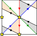
Refer to caption
(a) Double intersections.
Refer to caption
(b) Quadruple intersection.
Figure 15: Possible NS5 brane positions in the brane tiling describing the dP1𝑑subscript𝑃1dP_{1} orientifold singularity. The white regions are (N,0)𝑁0(N,0) branes and orange and grey regions are (N,1)𝑁1(N,1) and (N,1)𝑁1(N,-1) branes, respectively.
Refer to caption
(a) IAsubscriptI𝐴\mathrm{I}_{A}
Refer to caption
(b) IBsubscriptI𝐵\mathrm{I}_{B}
Refer to caption
(c) Unknown phase (II)
Refer to caption
(d) Unknown phase (III)
Figure 16: Local charges for the O5 planes in the four possible configurations T-dual to branes at the dP1𝑑subscript𝑃1dP_{1} orientifold singularity with the geometric involution described in the text. Configurations 16(a) and 16(b) correspond to the brane tiling in figure 15(a) and those in 16(c) and 16(d) to that in figure 15(b). The latter two are previously unknown phases.

By contrast, the configuration in figure 15(b) is non-standard, due to the quadruple intersection of NS5 branes at one of the fixed points. We emphasize that this quadruple intersection is forced on us by the O5 involution, which projected out the NS5 brane moduli which would otherwise allow us to deform away from this special point in the moduli space, see figure 17. Since this deformation grows a fourth (N,0)𝑁0(N,0) face in the brane tiling, the special point lies at infinite coupling for one of the gauge groups, and we expect that there are intrinsically strongly coupled degrees of freedom localized at the quadruple intersection. Thus, the answer to the paradox of §2 is that the missing phases are not gauge theories at all, but something intrinsically strongly coupled!
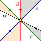
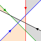
Refer to caption
(a) Four NS5 branes intersecting atop an O5 plane.
Refer to caption
(b) A deformation possible without the O5.
Refer to caption
(c) A different deformation possible without the O5.
Figure 17: 17(a) Four NS5 branes intersecting over a O5 plane. 17(b)17(c) Removing the orientifold plane, there are two deformations that allow a perturbative description, related by Seiberg duality.

In fact, as shown in figures 17(b) and 17(c), there are two ways in which the quadruple crossing can be resolved, related by Seiberg duality on the shrinking (N,0)𝑁0(N,0) face. A configuration with formally infinite coupling interpolating between two Seiberg dual phases is a familiar situation in the Hanany-Witten literature Hanany:1996ie ; Giveon:1998sr . However, the infinite coupling makes the gauge theory description ill-defined, and the orientifolds we consider lack a modulus to deform away from the strong-coupling point, so we need a different approach to describe the low-energy physics.

Let us take a step back and examine under what circumstances these higher multiplicity intersections are forced to occur. Since each NS5 brane crosses two fixed points, and there are four fixed points in total, it is evident that when there are more than four NS5 branes (i.e. more than four legs in the web diagram) a higher multiplicity intersection must occur at one or more of the fixed points, whereas in the case of four NS5 branes a quadruple intersection will occur for some choices of [H]delimited-[]𝐻[H], but not for others. This agrees exactly with what we found in §2, where there were no candidate duals for dP2𝑑subscript𝑃2dP_{2} and dP3𝑑subscript𝑃3dP_{3} and an incomplete list for dP1𝑑subscript𝑃1dP_{1} and 𝔽0subscript𝔽0\mathbb{F}_{0}. Moreover, in the case of three NS5 branes, as for all isolated orbifold singularities, a higher multiplicity intersection is obviously impossible, in perfect agreement with the precise matching between the discrete torsion classification of orbifolds and their dual gauge theories obtained in dualities1 ; dualities2 .

3.3 Quad CFTs

To isolate the physics associated to the quadruple crossing and to decouple details of the rest of the brane tiling, we zoom in on the vicinity of the O5 plane, replacing T2superscript𝑇2T^{2} with 2superscript2\mathbb{R}^{2}, so that the four (N,0)𝑁0(N,0) faces in figure 17(a) become flavor branes and the superpotential terms associated to the four (N,±1)𝑁plus-or-minus1(N,\pm 1) branes go to zero. The resulting brane configuration corresponds to a CFT in the infrared. Once these “quad” CFTs are understood, we can reintroduce gauge couplings for the non-compact branes by weakly gauging flavor symmetries of the CFT. Likewise, the missing superpotential terms can be reintroduced by deforming the CFT by a relevant operator.

Before orientifolding, the quadruple intersection can be resolved by a small deformation, as in figures 17(b)17(c), giving a pair of Seiberg dual gauge theories in the same universality class as the quad CFT, corresponding to the dimer models in figure 18(a). Heuristically, the orientifolded quad CFT corresponds to a quotient on the operator spectrum of this “parent” quad CFT. This is not quite correct, because the orientifold introduces a tadpole which must be cancelled by making ranks of the flavor branes unequal, but we expect it to be approximately true at large N𝑁N, where the difference in ranks is a small effect. Thus, we can learn something about the orientifolded quad CFT by studying its parent.

Refer to caption
(a) Dimer models for figures 17(b)17(c).
Refer to caption
(b) B-C brane recombination
Figure 18: 18(a) Dimer models for the Seiberg-dual deformations of the quadruple crossing, figures 17(b)17(c). 18(b) A partial resolution of the quadruple crossing in 17(a), which corresponds to turning on a vev where the B and C branes intersect in 17(b)17(c).

We use this technique to determine the flavor symmetries associated to the quadruple crossing. In addition to the SU(N)4𝑆𝑈superscript𝑁4SU(N)^{4} flavor symmetry associated to the flavor branes, there is an anomaly-free U(1)𝑈1U(1) flavor symmetry in the parent for each NS5 brane (zig-zag path) in the brane tiling Imamura:2006ie , where the sum of these U(1)𝑈1U(1)s decouples. Thus, the manifest non-R flavor symmetry group is SU(N)4×U(1)3𝑆𝑈superscript𝑁4𝑈superscript13SU(N)^{4}\times U(1)^{3}. However, the superpotential generated by the finite-area (N,±1)𝑁plus-or-minus1(N,\pm 1) faces in figures 17(b)17(c) respects a larger SU(2N)×SU(N)2×U(1)2𝑆𝑈2𝑁𝑆𝑈superscript𝑁2𝑈superscript12SU(2N)\times SU(N)^{2}\times U(1)^{2} flavor symmetry, where SU(2N)SU(N)2×U(1)𝑆𝑈superscript𝑁2𝑈1𝑆𝑈2𝑁SU(2N)\supset SU(N)^{2}\times U(1) is broken when the flavor branes are gauged, but is conserved by the quad CFT itself.

The orientifold projection maps the NS5 branes to themselves and exchanges the (N,0)𝑁0(N,0) flavor branes in pairs, hence the U(1)3𝑈superscript13U(1)^{3} subgroup is invariant, whereas the SU(N)𝑆𝑈𝑁SU(N) factors are exchanged in pairs, leaving the manifest flavor symmetry group SU(N)×SU(N+p)×U(1)3𝑆𝑈𝑁𝑆𝑈𝑁𝑝𝑈superscript13SU(N)\times SU(N+p)\times U(1)^{3} after orientifolding, where p𝑝p is the difference in ranks required to cancel the RR tadpole associated to the O5 plane. Thus, the orientifold projection maps the enhanced SU(2N)𝑆𝑈2𝑁SU(2N) symmetry of the parent theory to its charge conjugate, which suggests that SU(2N)𝑆𝑈2𝑁SU(2N) is broken to either SO(2N)𝑆𝑂2𝑁SO(2N) or USp(2N)𝑈𝑆𝑝2𝑁U\!Sp(2N) by the involution, where SO(2N)SU(N)×U(1)𝑆𝑈𝑁𝑈1𝑆𝑂2𝑁SO(2N)\supset SU(N)\times U(1) or USp(2N)SU(N)×U(1)𝑆𝑈𝑁𝑈1𝑈𝑆𝑝2𝑁U\!Sp(2N)\supset SU(N)\times U(1) is a nonabelian enhancement of the manifest flavor symmetries. This enhancement can be seen explicitly by Higgsing the baryon associated to the B-C crossing in figures 17(b)17(c), recombining the NS5 branes and giving the brane tiling shown in figure 18(b), which admits a perturbative, dimer model description. The superpotential terms associated to the finite-area (N,±1)𝑁plus-or-minus1(N,\pm 1) faces preserve the enhanced symmetry SO(2N)𝑆𝑂2𝑁SO(2N) (USp(2N)𝑈𝑆𝑝2𝑁U\!Sp(2N)) for an O5 plane of positive (negative) T-parity.

We infer that there are two classes of quad CFTs, depending on the overall sign of the RR charge of the O5 plane, with non-R flavor symmetry groups SO(2N)×SU(N+p)×U(1)2𝑆𝑂2𝑁𝑆𝑈𝑁𝑝𝑈superscript12SO(2N)\times SU(N+p)\times U(1)^{2} and USp(2N)×SU(N+p)×U(1)2𝑈𝑆𝑝2𝑁𝑆𝑈𝑁superscript𝑝𝑈superscript12U\!Sp(2N)\times SU(N+p^{\prime})\times U(1)^{2}, respectively, for p𝑝p and psuperscript𝑝p^{\prime} to be determined. We have also seen that these CFTs flow to an infrared-free theory with chiral superfields and a tree-level superpotential when we move along a baryonic branch corresponding to recombining the B and C NS5 branes. There are three other possible brane recombinations, shown in figure 19. In these cases, there are no finite-area (N,±1)𝑁plus-or-minus1(N,\pm 1) faces, hence the infrared physics is described by free chiral superfields.
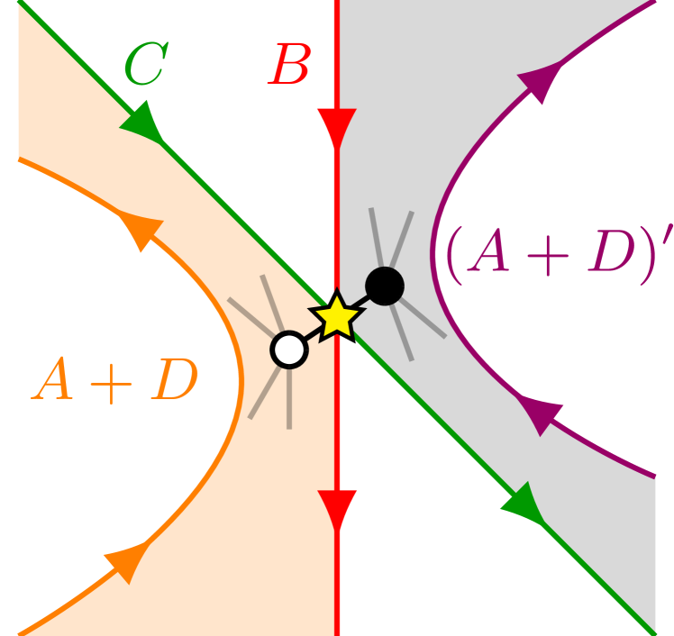
Refer to caption
(a) A-D recombination
Refer to caption
(b) B-D recombination
Refer to caption
(c) A-C recombination
Figure 19: Possible brane recombinations which resolve the quadruple crossing, in addition to the B-C recombination shown in figure 18(b). In each case, the corresponding dimer model is superimposed on the tiling.

These brane recombinations — which will correspond to partial resolutions of the toric singularity when the quad CFT is embedded into T2superscript𝑇2T^{2} — exhaust the baryonic directions in the moduli space. There are also mesonic directions coming from the gauge-singlet mesons in figure 18(a) and their orientifold images, which are composite mesons (elementary mesons in the Seiberg dual theory). Turning on a rank k𝑘k vev for the gauge-singlet mesons and their orientifold images, we obtain the rank Nk𝑁𝑘N-k quad CFT plus a residual U(k)2𝑈superscript𝑘2U(k)^{2} global symmetry and various gauge-singlet chiral superfields charged under SU(Nk)4×U(1)3×U(k)2𝑆𝑈superscript𝑁𝑘4𝑈superscript13𝑈superscript𝑘2SU(N-k)^{4}\times U(1)^{3}\times U(k)^{2}. These U(k)2𝑈superscript𝑘2U(k)^{2}-charged chiral fields do not appear in the superpotential, hence they decouple from the remainder of the quad CFT. When the quad CFT is embedded into T2superscript𝑇2T^{2}, this direction in moduli space will correspond to removing an orientifold image pair of stacks of k𝑘k D3 branes from the singularity without resolving it.

Thus, even without an explicit construction of the orientifolded quad CFTs, we can infer their global symmetries and the general characteristics of their moduli space. In the next section, we will construct CFTs which match these expectations, and are therefore candidate descriptions of the quadruple crossing.

4 Deconfinement and strong coupling

We now turn to the task of describing five-brane systems with quadruple intersections of NS5 branes, as in figure 15(b). We expect that these configurations are T-dual to configurations with the missing [H]delimited-[]𝐻[H] torsions in figure 12.

Surprisingly, even though (as we have argued) these configurations are intrinsically strongly coupled, it is still possible to construct a family of UV gauge theories in the same universality class as the strongly coupled theory. We motivate this through a brane engineering construction of the UV theories, and provide highly non-trivial evidence that our result is correct based on the quantum moduli space and superconformal index of the resulting theories, where the former matches with the five-brane description under the partial resolutions described in §3.3, and the latter passes all S-duality tests. Our construction is based on the deconfinement method of Berkooz:1995km ; Pouliot:1995me , which we now review.

4.1 Deconfinement in the gauge theory

Consider an USp(N4)𝑈𝑆𝑝𝑁4U\!Sp(N-4) gauge theory with N𝑁N chiral superfields Z^isuperscript^𝑍𝑖\hat{Z}^{i} in the vector representation, transforming under an SU(N)𝑆𝑈𝑁SU(N) flavor symmetry. It is well known Intriligator:1995ne that this theory s-confines with the composite Zij=ΩabZ^aiZ^bjsuperscript𝑍𝑖𝑗superscriptΩ𝑎𝑏subscriptsuperscript^𝑍𝑖𝑎subscriptsuperscript^𝑍𝑗𝑏Z^{ij}=\Omega^{ab}\hat{Z}^{i}_{a}\hat{Z}^{j}_{b} (where ΩabsuperscriptΩ𝑎𝑏\Omega^{ab} is the symplectic form of USp(N4)𝑈𝑆𝑝𝑁4U\!Sp(N-4)) and the superpotential

W=PfZ,𝑊Pf𝑍W=\operatorname{Pf}Z\,, (19)

where Z𝑍Z transforms in the representation of SU(N)𝑆𝑈𝑁SU(N). We consider deforming this theory by weakly gauging the SU(N)𝑆𝑈𝑁SU(N) flavor symmetry coupled to some set of additional chiral fields to cancel the anomalies. In the limit where the SU(N)𝑆𝑈𝑁SU(N) gauge coupling is small at the USp(N4)𝑈𝑆𝑝𝑁4U\!Sp(N-4) confinement scale, the low energy dynamics of this USp(N4)×SU(N)𝑈𝑆𝑝𝑁4𝑆𝑈𝑁U\!Sp(N-4)\times SU(N) gauge theory are the same as those of the SU(N)𝑆𝑈𝑁SU(N) gauge theory with the s-confined matter spectrum and superpotential (19). We can construct further duals of this theory by considering the limit where the SU(N)𝑆𝑈𝑁SU(N) gauge coupling becomes large before the USp(N4)𝑈𝑆𝑝𝑁4U\!Sp(N-4) confinement scale. If there is no phase transition in between and the IR fixed point is isolated, this theory describes the same infrared physics as before. In the limit where the USp(N4)𝑈𝑆𝑝𝑁4U\!Sp(N-4) gauge coupling is small at the SU(N)𝑆𝑈𝑁SU(N) dynamical scale, we can replace SU(N)𝑆𝑈𝑁SU(N) with its Seiberg dual to obtain another theory with the same infrared fixed point. By dualizing nodes of the quiver in turn, we obtain a chain of dual descriptions Berkooz:1995km . This “deconfinement” technique is helpful for understanding the dynamics of the original SU(N)𝑆𝑈𝑁SU(N) gauge theory with antisymmetric tensor matter.

So far we have assumed that the SU(N)𝑆𝑈𝑁SU(N) gauge theory in question has a superpotential in the infrared of the form (19). To describe a theory without a superpotential, we replace USp(N4)𝑈𝑆𝑝𝑁4U\!Sp(N-4) with USp(N+F4)𝑈𝑆𝑝𝑁𝐹4U\!Sp(N+F-4) in the UV theory for some arbitrary F>0𝐹0F>0, and add F𝐹F additional USp(N+F4)𝑈𝑆𝑝𝑁𝐹4U\!Sp(N+F-4) vectors P𝑃P transforming under an SU(F)𝑆𝑈𝐹SU(F) flavor symmetry, as well as F𝐹F antifundamentals Q𝑄Q of SU(N)𝑆𝑈𝑁SU(N) transforming under the same SU(F)𝑆𝑈𝐹SU(F) and a gauge-singlet T𝑇T in the representation of SU(F)𝑆𝑈𝐹SU(F). This gives the quiver diagram shown in figure 20. We introduce the SU(F)𝑆𝑈𝐹SU(F)-invariant superpotential

W=PQZ^+TP2.𝑊𝑃𝑄^𝑍𝑇superscript𝑃2W=PQ\hat{Z}+TP^{2}\,. (20)

When the USp(N+F4)𝑈𝑆𝑝𝑁𝐹4U\!Sp(N+F-4) theory s-confines, it forms the composites

M=(Z^2Z^PZ^PP2)𝑀matrixsuperscript^𝑍2^𝑍𝑃^𝑍𝑃superscript𝑃2M=\begin{pmatrix}\hat{Z}^{2}&\hat{Z}P\\ -\hat{Z}P&P^{2}\end{pmatrix} (21)

with the confining superpotential PfMPf𝑀\operatorname{Pf}M. However, Z^P^𝑍𝑃\hat{Z}P and P2superscript𝑃2P^{2} get a mass with Q𝑄Q and T𝑇T respectively, via the tree-level superpotential (20), and can be integrated out. The F𝐹F-term conditions for Q𝑄Q and T𝑇T set Z^P=P2=0^𝑍𝑃superscript𝑃20\hat{Z}P=P^{2}=0, and the confining superpotential vanishes, leaving behind a single SU(N)𝑆𝑈𝑁SU(N) antisymmetric tensor Z=Z^2𝑍superscript^𝑍2Z=\hat{Z}^{2} with no superpotential Pouliot:1995me .
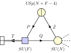
Refer to caption
Figure 20: Deconfined description for an antisymmetric tensor.

Note that the choice of F>0𝐹0F>0 is arbitrary, except that N+F𝑁𝐹N+F must be even for USp(N+F4)𝑈𝑆𝑝𝑁𝐹4U\!Sp(N+F-4) to exist. In the infrared, no fields are charged under the SU(F)𝑆𝑈𝐹SU(F). Thus, despite being unbroken, the UV symmetry SU(F)𝑆𝑈𝐹SU(F) is not a symmetry of the infrared fixed point, explaining how theories with different global symmetry groups in the UV and no accidental symmetries can describe the same infrared physics. We refer to such a UV global symmetry as “trivial”.

In fact, the triviality of SU(F)𝑆𝑈𝐹SU(F) imposes interesting a posteriori constraints on the moduli space and operator spectrum. Consider turning on a vev for a gauge-invariant operator in a non-trivial SU(F)𝑆𝑈𝐹SU(F) representation, spontaneously breaking the SU(F)𝑆𝑈𝐹SU(F). In the UV theory, this is a D-flat direction classically, and it is straightforward to choose an operator which also satisfies the classical F-term constraints such as T𝑇T (for F>2𝐹2F>2, so that T𝑇T transforms under SU(F)𝑆𝑈𝐹SU(F)). However, triviality for SU(F)𝑆𝑈𝐹SU(F) implies that the operator in question is lifted in the infrared, hence it is not a flat direction of the full theory. This is true for any operator in a non-trivial SU(F)𝑆𝑈𝐹SU(F) representation. Thus, for most practical purposes, we can treat SU(F)𝑆𝑈𝐹SU(F) as weakly gauged, and only consider SU(F)𝑆𝑈𝐹SU(F) singlet operators. Triviality of the SU(F)𝑆𝑈𝐹SU(F) implies the vanishing of the SU(F)3𝑆𝑈superscript𝐹3SU(F)^{3} and SU(F)2U(1)𝑆𝑈superscript𝐹2𝑈1SU(F)^{2}U(1) anomalies, except that SU(F)2U(1)R𝑆𝑈superscript𝐹2𝑈subscript1𝑅SU(F)^{2}U(1)_{R} receives a contribution from the SU(F)𝑆𝑈𝐹SU(F) gauginos, and the R-symmetry is anomalous. Since the SU(F)𝑆𝑈𝐹SU(F) is trivial, once gauged it undergoes gaugino condensation in the infrared, resulting in F𝐹F isolated vacua in the SU(F)𝑆𝑈𝐹SU(F) sector, and an accidental R-symmetry in the SU(N)𝑆𝑈𝑁SU(N) sector. While this is essentially (though not exactly) equivalent to the infrared physics of the theory before gauging the SU(F)𝑆𝑈𝐹SU(F), it is usually more convenient to treat SU(F)𝑆𝑈𝐹SU(F) as a global symmetry, keeping in mind that it is trivial, hence only SU(F)𝑆𝑈𝐹SU(F) singlets contribute to the IR dynamics.

To illustrate the triviality of SU(F)𝑆𝑈𝐹SU(F), we consider the effect of a few SU(F)𝑆𝑈𝐹SU(F)-breaking vevs. Turning on a vev for T𝑇T gives mass to some of the P𝑃P’s. If T𝑇T has rank greater than one, then USp(N+F4)𝑈𝑆𝑝𝑁𝐹4U\!Sp(N+F-4) develops a dynamical superpotential, and supersymmetry is broken. If T𝑇T has rank one and F>2𝐹2F>2, USp(N+F4)𝑈𝑆𝑝𝑁𝐹4U\!Sp(N+F-4) has a quantum-deformed moduli space, PfM=ΛN+F2Pf𝑀superscriptΛ𝑁𝐹2\operatorname{Pf}M=\Lambda^{N+F-2}, but the F-term conditions set PfM=0Pf𝑀0\operatorname{Pf}M=0 as before, so supersymmetry is broken. If T𝑇T has rank one and F=2𝐹2F=2, then T𝑇T is a SU(F)𝑆𝑈𝐹SU(F) singlet, and the result is different. After integrating out the P𝑃P’s in the UV theory, we are left with a superpotential W=Q2Z^2𝑊superscript𝑄2superscript^𝑍2W=Q^{2}\hat{Z}^{2}. As before, USp(N+F4)𝑈𝑆𝑝𝑁𝐹4U\!Sp(N+F-4) has a quantum-deformed moduli space Pf(Z^2)=ΛN+F2Pfsuperscript^𝑍2superscriptΛ𝑁𝐹2\operatorname{Pf}(\hat{Z}^{2})=\Lambda^{N+F-2}, but now the F-term conditions do not enforce Pf(Z^2)=0Pfsuperscript^𝑍20\operatorname{Pf}(\hat{Z}^{2})=0. Instead, SU(N)𝑆𝑈𝑁SU(N) is Higgsed to USp(N)𝑈𝑆𝑝𝑁U\!Sp(N) and Q𝑄Q acquires a mass, leaving SU(F)𝑆𝑈𝐹SU(F) trivial as before.212121In fact, T𝑇T plays the same role in this case as Z^N=PfZsuperscript^𝑍𝑁Pf𝑍\hat{Z}^{N}=\operatorname{Pf}Z does for even N𝑁N and F4𝐹4F\geq 4 (Z^Nsuperscript^𝑍𝑁\hat{Z}^{N} vanishes identically for F=2𝐹2F=2). A similar story applies to other SU(F)𝑆𝑈𝐹SU(F) breaking directions in the classical moduli space.

4.2 Deconfinement in the brane tiling

In this section, we engineer deconfinement of an antisymmetric tensor in the five-brane system discussed in §3.2. In the process, we will inevitably encounter non-BPS — indeed, dynamically unstable — brane configurations. This situation is not unprecedented. For instance, many of the toric phases which arise in dimer models cannot be realized by brane tilings with straight NS5 branes. These “geometrically inconsistent” phases Broomhead:2008an ; Hanany:2006nm do not correspond to any BPS configuration of branes, but in general they are Seiberg-dual to some geometrically consistent phase, hence they lie in the same universality class as some BPS configuration. With this example in mind, we engineer a configuration of branes which reproduces the gauge theory construction of §4.1, ignoring issues of supersymmetry and stability. We then provide some post hoc justification for why this works.

We start with the brane tiling description of a single antisymmetric tensor multiplet of SU(N)𝑆𝑈𝑁SU(N), see figure 14. As in §3.3, we take the worldvolume of the D5 branes to be 2superscript2\mathbb{R}^{2} instead of T2superscript𝑇2T^{2}, so that there is a single O5 plane, and the image pair of (N,0)𝑁0(N,0) faces corresponds to an SU(N)𝑆𝑈𝑁SU(N) flavor symmetry. The O5 plane is divided into an O5+ plane and an O5- plane by the NS5 branes, with opposite D5 charges in the two parts, so the NS5 branes carry D5 charge ±2plus-or-minus2\pm 2 to cancel the tadpole Imamura:2008fd .

Leaving aside the issue of flavors and the confining superpotential temporarily, deconfinement has an obvious description in the dimer model, see figure 21(a). The antisymmetric tensor corresponds to an edge crossing a fixed point of negative T-parity. To deconfine this tensor, we replace the edge with an image-pair of edges surrounding a two-sided face with the fixed point in the middle. The new face is an USp𝑈𝑆𝑝U\!Sp gauge group — USp(N4)𝑈𝑆𝑝𝑁4U\!Sp(N-4) by anomaly cancellation — which s-confines, reproducing the antisymmetric tensor we started with. Thus, deconfinement corresponds to “doubling” in the language of Davey:2009bp ; Davey:2011sw .
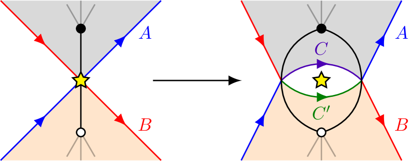
Refer to caption
(a) Deconfinement in the dimer
Refer to caption
(b) Triple crossing of NS5 branes
Figure 21: 21(a) Deconfinement corresponds to edge doubling in the dimer model. To avoid a global change in the structure of the zig-zag paths, the original paths A𝐴A and B𝐵B are forced to recombine into new paths C𝐶C and Csuperscript𝐶C^{\prime} on the doubled edges. 21(b) The configuration of branes prior to “lifting”, with a triple crossing of NS5 branes. The dashed line indicates the boundary of the region to be lifted off the D5 stack, and the shaded regions within this line will become the NS5 branes C𝐶C and Csuperscript𝐶C^{\prime}.

In order to translate this into a five-brane system, we construct the zig-zag paths of the dimer. This immediately leads to a puzzle: before doubling the edge, there are two zig-zag paths, A𝐴A and B𝐵B, which cross at the fixed point. After doubling, one end of A𝐴A connects to the other end of B𝐵B, and vice versa, so the zig-zag paths get reconnected, even though we performed a local operation in the dimer. Taking the new zig-zag paths literally leads to the conclusion that dimer models of this type are “inconsistent” Hanany:2005ss .

Instead, we interpret the two zig-zag paths inside the new two-sided face as new NS5 branes C𝐶C and Csuperscript𝐶C^{\prime} which appear after deconfinement, whereas the zig-zag paths outside the new face are the same NS5 branes A𝐴A and B𝐵B that were present before deconfinement. To understand how the two halves of A𝐴A and B𝐵B are joined together and how C𝐶C and Csuperscript𝐶C^{\prime} connect to A𝐴A and B𝐵B, we construct the entire NS5 brane configuration in two steps, as follows. First, we deform the initial brane configuration by changing the single crossing of the NS5 branes into a triple crossing, creating an image pair of “eyes” surrounding the O5 plane, as in figure 21(b). We then trace out a contour enclosing this pair of eyes, and lift the NS5 branes within the enclosing contour off of the D5 stack into the minor angle between the A𝐴A and B𝐵B branes in the (x6,x7)subscript𝑥6subscript𝑥7(x_{6},x_{7}) plane, opening up a “bubble” bounded by a new (N4,0)𝑁40(N-4,0) face on the D5 stack and the lifted NS5 branes, which we identify as C𝐶C and Csuperscript𝐶C^{\prime}. The NS5 branes A𝐴A and B𝐵B now end on the upper surface of the bubble, tracing out the same double eye as before, where they fuse with the upper boundary of the branes C𝐶C and Csuperscript𝐶C^{\prime}.

Refer to caption
(a) The D5 worldvolume
Refer to caption
(b) The top of the bubble
Refer to caption
(c) The O5 worldvolume
Figure 22: The configuration of branes after lifting, including the pair creation of F𝐹F flavor branes. We use the same orientation conventions in 22(a) and 22(b), so that the flavor faces on the roof of the bubble appear here as (F,0)𝐹0(-F,0), which is the same as (F,0)𝐹0(F,0) oppositely oriented.

We add F𝐹F flavors to this configuration by pair-creating F𝐹F pairs of D5 branes within the larger eye and adding half of these to the USp(N4)𝑈𝑆𝑝𝑁4U\!Sp(N-4) face to obtain USp(N+F4)𝑈𝑆𝑝𝑁𝐹4U\!Sp(N+F-4). Their F𝐹F opposite numbers are bound to the NS5 branes C𝐶C and Csuperscript𝐶C^{\prime} on the roof of the bubble, where they fill in the pair of eyes created by the boundaries of the branes A𝐴A and B𝐵B, generating (F,0)𝐹0(F,0) faces (oriented oppositely to the (N+F4,0)𝑁𝐹40(N+F-4,0) face below them) with a corresponding SU(F)𝑆𝑈𝐹SU(F) symmetry. The final brane configuration is illustrated in figure 22.

For completeness, we construct an explicit realization of the “deconfinement bubble” described above. This is done merely to better illustrate our argument; we emphasize that the details of the curves have no effect on our conclusions.

We take the initial configuration of branes to be x5=±x4subscript𝑥5plus-or-minussubscript𝑥4x_{5}=\pm x_{4} and x7=±x6subscript𝑥7plus-or-minussubscript𝑥6x_{7}=\pm x_{6}, x60subscript𝑥60x_{6}\geq 0, where the upper (lower) sign applies to brane A𝐴A (brane B𝐵B) and the D5 stack is located at x6=x7=0subscript𝑥6subscript𝑥70x_{6}=x_{7}=0.222222Here we have fixed the minor angle between the branes to be 90superscript9090^{\circ}, but this can easily be changed. We then deform the branes to create a triple crossing as in figure 21(b), so that their boundaries lie at x5=±x4x42/a21x42/a2+1subscript𝑥5plus-or-minussubscript𝑥4superscriptsubscript𝑥42superscript𝑎21superscriptsubscript𝑥42superscript𝑎21x_{5}=\pm x_{4}\frac{x_{4}^{2}/a^{2}-1}{x_{4}^{2}/a^{2}+1}, where a𝑎a controls the size of the deformation in the (x4,x5)subscript𝑥4subscript𝑥5(x_{4},x_{5}) plane. The deformation can be extended into the bulk as

x5=±x4x42/a2+x62/b21x42/a2+x62/b2+1,subscript𝑥5plus-or-minussubscript𝑥4superscriptsubscript𝑥42superscript𝑎2superscriptsubscript𝑥62superscript𝑏21superscriptsubscript𝑥42superscript𝑎2superscriptsubscript𝑥62superscript𝑏21x_{5}=\pm x_{4}\frac{x_{4}^{2}/a^{2}+x_{6}^{2}/b^{2}-1}{x_{4}^{2}/a^{2}+x_{6}^{2}/b^{2}+1}\,, (22)

where b𝑏b controls the size of the deformation in the (x6,x7)subscript𝑥6subscript𝑥7(x_{6},x_{7}) plane, so that the branes return to their initial shapes asymptotically as x4,x6subscript𝑥4subscript𝑥6x_{4},x_{6}\to\infty.

Next, we trace out an eye surrounding the triple crossing at x5=±a2[1x42/a2]subscript𝑥5plus-or-minus𝑎2delimited-[]1superscriptsubscript𝑥42superscript𝑎2x_{5}=\pm\frac{a}{2}[1-x_{4}^{2}/a^{2}] for |x4|asubscript𝑥4𝑎|x_{4}|\leq a. After the lift, this describes boundary of the brane C𝐶C (Csuperscript𝐶C^{\prime}) for the upper (lower) sign, and is chosen to match first derivatives with the boundaries of A𝐴A and B𝐵B at their mutual intersections. To implement the lift, we specify the displacement of C𝐶C, Csuperscript𝐶C^{\prime} in the positive x6subscript𝑥6x_{6} direction by

x52/a2+[1x42/a2]x62/c2=14[1x42/a2]2superscriptsubscript𝑥52superscript𝑎2delimited-[]1superscriptsubscript𝑥42superscript𝑎2superscriptsubscript𝑥62superscript𝑐214superscriptdelimited-[]1superscriptsubscript𝑥42superscript𝑎22x_{5}^{2}/a^{2}+[1-x_{4}^{2}/a^{2}]\,x_{6}^{2}/c^{2}=\frac{1}{4}[1-x_{4}^{2}/a^{2}]^{2} (23)

for |x4|asubscript𝑥4𝑎|x_{4}|\leq a, where c𝑐c controls the size of the lift and the x4subscript𝑥4x_{4}-dependent prefactor of x62superscriptsubscript𝑥62x_{6}^{2} is chosen for later convenience. The branes C𝐶C, Csuperscript𝐶C^{\prime} stretch between their boundaries on the D5 branes at x5=±a2[1x42/a2]subscript𝑥5plus-or-minus𝑎2delimited-[]1superscriptsubscript𝑥42superscript𝑎2x_{5}=\pm\frac{a}{2}[1-x_{4}^{2}/a^{2}] and their intersection with the branes A𝐴A and B𝐵B, along the pair of curves specified by

x42/a2x42/a2+x62/b21x42/a2+x62/b2+1+[1x42/a2]x62/c2=14[1x42/a2]2,superscriptsubscript𝑥42superscript𝑎2superscriptsubscript𝑥42superscript𝑎2superscriptsubscript𝑥62superscript𝑏21superscriptsubscript𝑥42superscript𝑎2superscriptsubscript𝑥62superscript𝑏21delimited-[]1superscriptsubscript𝑥42superscript𝑎2superscriptsubscript𝑥62superscript𝑐214superscriptdelimited-[]1superscriptsubscript𝑥42superscript𝑎22x_{4}^{2}/a^{2}\,\frac{x_{4}^{2}/a^{2}+x_{6}^{2}/b^{2}-1}{x_{4}^{2}/a^{2}+x_{6}^{2}/b^{2}+1}+[1-x_{4}^{2}/a^{2}]\,x_{6}^{2}/c^{2}=\frac{1}{4}[1-x_{4}^{2}/a^{2}]^{2}\,, (24)

where we choose c<2b𝑐2𝑏c<2b so that the branes intersect before the pair of eyes surrounding the O5 plane close up. The final configuration of branes in the (x4,x5,x6)subscript𝑥4subscript𝑥5subscript𝑥6(x_{4},x_{5},x_{6}) directions is plotted in figure 23(a).
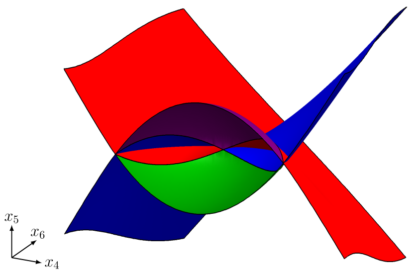
Refer to caption
(a) The (x4,x5,x6)subscript𝑥4subscript𝑥5subscript𝑥6(x_{4},x_{5},x_{6}) directions
Refer to caption
(b) The (x4,x6,x7)subscript𝑥4subscript𝑥6subscript𝑥7(x_{4},x_{6},x_{7}) directions
Figure 23: The deconfined NS5 branes, plotted using the equations described in the text (for c=2b𝑐2𝑏c=\sqrt{2}b). The flavor branes are not pictured: they fill in the pair of eyes where the branes A𝐴A and B𝐵B intersect the branes C𝐶C and Csuperscript𝐶C^{\prime}.

We now describe the positions of the branes in the x7subscript𝑥7x_{7} direction. Before lifting, we had x7=±x6subscript𝑥7plus-or-minussubscript𝑥6x_{7}=\pm x_{6} for branes A𝐴A and B𝐵B, respectively. In order to match the slopes of the branes A𝐴A and B𝐵B with C𝐶C and Csuperscript𝐶C^{\prime} at their intersection point on the D5 stack, we choose x7=x4ax6subscript𝑥7minus-or-plussubscript𝑥4𝑎subscript𝑥6x_{7}=\mp\frac{x_{4}}{a}x_{6} for C𝐶C and Csuperscript𝐶C^{\prime}, respectively. To ensure that A𝐴A and B𝐵B meet the boundary of C𝐶C and Csuperscript𝐶C^{\prime} along the curve (24), we deform the x7subscript𝑥7x_{7} position of A𝐴A and B𝐵B by:

x72/c2=x62/c2+x52/a214[1x42/a2]2,superscriptsubscript𝑥72superscript𝑐2superscriptsubscript𝑥62superscript𝑐2superscriptsubscript𝑥52superscript𝑎214superscriptdelimited-[]1superscriptsubscript𝑥42superscript𝑎22x_{7}^{2}/c^{2}=x_{6}^{2}/c^{2}+x_{5}^{2}/a^{2}-\frac{1}{4}[1-x_{4}^{2}/a^{2}]^{2}\,, (25)

for |x4|<asubscript𝑥4𝑎|x_{4}|<a, where brane A𝐴A (B𝐵B) correspond to the x7>0subscript𝑥70x_{7}>0 (x7<0subscript𝑥70x_{7}<0) branch of the solution. This reproduces x72=x42a2x62superscriptsubscript𝑥72superscriptsubscript𝑥42superscript𝑎2superscriptsubscript𝑥62x_{7}^{2}=\frac{x_{4}^{2}}{a^{2}}x_{6}^{2} on the intersection with (23) and reduces to x7=±x6subscript𝑥7plus-or-minussubscript𝑥6x_{7}=\pm x_{6} in the x6subscript𝑥6x_{6}\to\infty limit. Setting x42=a2superscriptsubscript𝑥42superscript𝑎2x_{4}^{2}=a^{2}, we obtain x72/c2=x62/c2+x52/a2superscriptsubscript𝑥72superscript𝑐2superscriptsubscript𝑥62superscript𝑐2superscriptsubscript𝑥52superscript𝑎2x_{7}^{2}/c^{2}=x_{6}^{2}/c^{2}+x_{5}^{2}/a^{2}, which differs slightly from the initial configuration x7=±x6subscript𝑥7plus-or-minussubscript𝑥6x_{7}=\pm x_{6} because x5=±ax62/b2x62/b2+10subscript𝑥5plus-or-minus𝑎superscriptsubscript𝑥62superscript𝑏2superscriptsubscript𝑥62superscript𝑏210x_{5}=\pm a\frac{x_{6}^{2}/b^{2}}{x_{6}^{2}/b^{2}+1}\neq 0. In order to match onto this behavior for |x4|>asubscript𝑥4𝑎|x_{4}|>a, we take

x72/c2=x62/c2+[3x42/a22][2x42/a2+x62/b22]x62/b2[x42/a2+x62/b2+1]2x44/a4,superscriptsubscript𝑥72superscript𝑐2superscriptsubscript𝑥62superscript𝑐2delimited-[]3superscriptsubscript𝑥42superscript𝑎22delimited-[]2superscriptsubscript𝑥42superscript𝑎2superscriptsubscript𝑥62superscript𝑏22superscriptsubscript𝑥62superscript𝑏2superscriptdelimited-[]superscriptsubscript𝑥42superscript𝑎2superscriptsubscript𝑥62superscript𝑏212superscriptsubscript𝑥44superscript𝑎4x_{7}^{2}/c^{2}=x_{6}^{2}/c^{2}+\frac{[3x_{4}^{2}/a^{2}-2][2x_{4}^{2}/a^{2}+x_{6}^{2}/b^{2}-2]\,x_{6}^{2}/b^{2}}{[x_{4}^{2}/a^{2}+x_{6}^{2}/b^{2}+1]^{2}\,x_{4}^{4}/a^{4}}\,, (26)

for |x4|>asubscript𝑥4𝑎|x_{4}|>a, where the second term is chosen to match first derivatives at |x4|=asubscript𝑥4𝑎|x_{4}|=a and to reproduce x7±x6subscript𝑥7plus-or-minussubscript𝑥6x_{7}\to\pm x_{6} asymptotically as x4,x6subscript𝑥4subscript𝑥6x_{4},x_{6}\to\infty. The final configuration of branes in the (x4,x6,x7)subscript𝑥4subscript𝑥6subscript𝑥7(x_{4},x_{6},x_{7}) directions is plotted in figure 23(b).

With a complete picture of the deconfined configuration of NS5 branes, we can read off the physics of the resulting gauge theory. From the perspective of the D5 stack near the intersection of branes A𝐴A and B𝐵B, the F𝐹F flavor branes are ordinary minor flavor branes Franco:2006es ; Imamura:2008fd . Thus, in addition to the bifundamental Z^^𝑍\hat{Z} usually generated at the intersection point, flavored fields P𝑃P and Q𝑄Q are also present, and there is a superpotential term Z^PQ^𝑍𝑃𝑄\hat{Z}PQ, as in (20). Similarly, from the perspective of the F𝐹F flavor branes near their intersection with the O5 plane, they form part of an ordinary brane tiling, hence by analogy there is an antisymmetric tensor T𝑇T of SU(F)𝑆𝑈𝐹SU(F) at the point of intersection with the O5 plane. By the same analogy, the image pair of NS5 branes C𝐶C and Csuperscript𝐶C^{\prime} will generate a superpotential term TP2𝑇superscript𝑃2TP^{2} formed from the fields encircling their perimeter.

Thus, the configuration of branes constructed above completely reproduces the deconfined theory of §4.1, with one exception: since the (F,0)𝐹0(F,0) flavor faces have finite size, the SU(F)𝑆𝑈𝐹SU(F) flavor symmetry is gauged. As noted in §4.1, this describes almost the same physics as an ungauged, trivial SU(F)𝑆𝑈𝐹SU(F). However, it is more convenient to work with a global SU(F)𝑆𝑈𝐹SU(F), and this is easily engineered by “puncturing” the (F,0)𝐹0(F,0) faces, i.e. by attaching long thin D5-brane tubes which end at infinity. When the USp(N+F4)𝑈𝑆𝑝𝑁𝐹4U\!Sp(N+F-4) face confines, the SU(F)𝑆𝑈𝐹SU(F) flavor tubes pinch off, leaving behind a trivial SU(F)𝑆𝑈𝐹SU(F) flavor symmetry, as in the gauge theory description.

We conclude that the above non-BPS, unstable configuration of branes — which is a small deformation of the initial, BPS configuration — produces an 𝒩=1𝒩1\mathcal{N}=1 gauge theory in the right universality class when we naively ignore the supersymmetry-breaking couplings. We can explain this heuristically as follows: we imagine deforming the full string theory by coupling it to external currents sourcing F-term tadpoles for the transverse scalars of the branes, arranged so that the deformed theory relaxes into the configuration of curved branes we are interested in, which is now supersymmetric due to the F-term tadpoles. In general, this deformed theory will not be UV complete, but since we are interested in the infrared physics, we ignore this and consider the effect of the deformation on the infrared fixed point. Let us suppose that the deformed theory has the same flavor symmetries as the undeformed theory, without any accidental symmetries.232323Non-abelian (rank-preserving) symmetry enhancements, such as occur in §4.4, do not affect this reasoning. In this case, the superconformal R-symmetry in the IR is a conserved symmetry of the UV theory, and the UV deformation can only induce marginal deformations in the IR. Since these deformations are forced to be flavor singlets, they are exactly marginal Green:2010da , and the deformed theory will flow to the same conformal manifold as the undeformed theory. In particular, in the absence of exactly marginal deformations, the two theories are in the same universality class.

Leaving aside the subtleties of this heuristic reasoning, let us see how it applies to the case at hand. Introducing the above deconfinement bubble without flavor branes (F=0𝐹0F=0) leads to a deformed theory with fewer flavor symmetries, due to the USp(N4)2U(1)𝑈𝑆𝑝superscript𝑁42𝑈1U\!Sp(N-4)^{2}U(1) mixed anomalies, and we expect that the infrared physics may differ from that of the original brane configuration. Indeed, the USp(N4)𝑈𝑆𝑝𝑁4U\!Sp(N-4) s-confines and generates a confining superpotential (19) not present in the initial theory.242424In the case where SU(N)𝑆𝑈𝑁SU(N) is not gauged, this superpotential is irrelevant in the IR, but this is not true in general when SU(N)𝑆𝑈𝑁SU(N) is gauged. Conversely, once we add flavor branes to the deconfinement bubble in the manner described above, the symmetries of the deformed theory match those of the original theory, and indeed the infrared physics of the two descriptions match, as shown in §4.1.

Thus, by matching the flavor symmetries of the deformed and undeformed brane configurations, we gain some control over changes to the infrared physics. With this in mind, we apply the same deconfinement construction to understand the quadruple crossing of NS5 branes encountered in §3.2.

4.3 Deconfining phase II

We are interested in the local physics of four NS5 branes intersecting atop an O5 plane, as in figure 24. As above, we begin by considering the case of non-compact D5 branes with an single O5 plane in the middle, corresponding to the “quad CFTs” considered in §3.3. The deformations corresponding to deconfinement are local, so that once this configuration is understood there is no obstacle to embedding it into T2superscript𝑇2T^{2}.

Refer to caption
(a) x6=x7=0subscript𝑥6subscript𝑥70x_{6}=x_{7}=0 plane
Refer to caption
(b) O5 structure in phase II
Refer to caption
(c) O5 structure in phase III
Figure 24: Neighborhood of the strongly coupled sector in phases II and III of the dP1𝑑subscript𝑃1dP_{1} orientifold.

There are two phases to consider, differing by an overall sign in the local RR charges of the O5 plane. In this section, we focus on the case shown in figure 24(b). Because we will only deconfine antisymmetric (rather than symmetric) tensors, the case shown in figure 24(c) is somewhat different, and will be treated separately in §4.4.

In the same spirit as §4.2, we can imagine pairing any two adjacent legs of the web diagram and blowing up a deconfinement bubble by recombining the associated NS5 branes. Analogous to deconfinement of an antisymmetric tensor, we choose to pair only legs that enclose an O5 plane with positive charge in their minor angle. Thus, for phase II we can either recombine B𝐵B and C𝐶C or recombine A𝐴A and D𝐷D. We consider the former combination for now, returning to the latter shortly. After recombination, the brane configuration is the same as in §4.2, but with the branes A𝐴A and D𝐷D superimposed on top, see figure 25. Since the deconfinement bubble is contained within the minor angle between branes B𝐵B and C𝐶C, A𝐴A and D𝐷D do not intersect it off the D5 brane stack. Moreover, the quadruple intersection has been resolved, and we can read off the resulting gauge theory exactly as in §3.2, accounting for the flavor branes as in the same way as in §4.2.
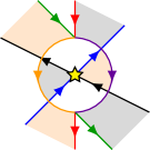
Refer to caption
(a) The D5 worldvolume
Refer to caption
(b) The O5 worldvolume
Refer to caption
(c) Quiver diagram
Figure 25: Local picture for the deconfinement in phase II obtained by deforming B𝐵B and C𝐶C together. In 25(b) the intersection of the O5 with the x6=x7=0subscript𝑥6subscript𝑥70x_{6}=x_{7}=0 plane where the tiling lives is indicated by the yellow circle. After deconfinement the B𝐵B and C𝐶C branes no longer intersect over this point (they rather intersect over the flavor stack, indicated by the blue square), but A𝐴A and D𝐷D still do.

The resulting quiver gauge theory is shown in figure 25(c), and the corresponding charge table is shown in table 4, where the tree-level superpotential is

W=A1A2Z+YPQ+TQ2Z.𝑊subscript𝐴1subscript𝐴2𝑍𝑌𝑃𝑄𝑇superscript𝑄2𝑍W=A_{1}A_{2}Z+YPQ+TQ^{2}Z\,. (27)

The a𝑎a-maximized R-charge Intriligator:2003jj is

U(1)R(sc)=U(1)R+(43+M4(αM1)2+αM(αM2))U(1)B+αMU(1)Y,𝑈superscriptsubscript1𝑅sc𝑈subscript1𝑅43𝑀4superscriptsubscript𝛼𝑀12subscript𝛼𝑀subscript𝛼𝑀2𝑈subscript1𝐵subscript𝛼𝑀𝑈subscript1𝑌U(1)_{R}^{\rm(sc)}=U(1)_{R}+\left(-\frac{4}{3}+\frac{M}{4}(\alpha_{M}-1)^{2}+\alpha_{M}(\alpha_{M}-2)\right)U(1)_{B}+\alpha_{M}U(1)_{Y}\,, (28)

where αMsubscript𝛼𝑀\alpha_{M} is the smallest non-negative root of

9(M+4)αM39MαM23(3M+4)αM+M=0.9𝑀4superscriptsubscript𝛼𝑀39𝑀superscriptsubscript𝛼𝑀233𝑀4subscript𝛼𝑀𝑀09(M+4)\alpha_{M}^{3}-9M\alpha_{M}^{2}-3(3M+4)\alpha_{M}+M=0\,. (29)
SU(M+F)SU(M)SU(M+4)SU(F)U(1)BU(1)XU(1)YU(1)RA1¯ 𝟏𝟏1M+F1M+4M+F12M+FA2¯ ¯ 𝟏𝟏1M+F1M+4M+F12M+FY 𝟏¯ 𝟏1M+F01+M+4M+F2M+FZ 𝟏𝟏𝟏2M+F02(M+4)M+F4M+FP𝟏𝟏 ¯ 1F012Q¯ 𝟏𝟏 1M+F1F0M+4M+F2M+FT𝟏𝟏𝟏¯ 2F002missing-subexpression𝑆𝑈𝑀𝐹𝑆𝑈𝑀𝑆𝑈𝑀4𝑆𝑈𝐹𝑈subscript1𝐵𝑈subscript1𝑋𝑈subscript1𝑌𝑈subscript1𝑅missing-subexpressionmissing-subexpressionmissing-subexpressionmissing-subexpressionmissing-subexpressionmissing-subexpressionmissing-subexpressionmissing-subexpressionmissing-subexpressionsubscript𝐴1¯absent 111𝑀𝐹1𝑀4𝑀𝐹12𝑀𝐹subscript𝐴2¯absent ¯absent 111𝑀𝐹1𝑀4𝑀𝐹12𝑀𝐹𝑌 1¯absent 11𝑀𝐹01𝑀4𝑀𝐹2𝑀𝐹𝑍 1112𝑀𝐹02𝑀4𝑀𝐹4𝑀𝐹𝑃11 ¯absent 1𝐹012𝑄¯absent 11 1𝑀𝐹1𝐹0𝑀4𝑀𝐹2𝑀𝐹𝑇111¯absent 2𝐹002\begin{array}[]{c|c|ccccccc}&SU(M+F)&SU(M)&SU(M+4)&SU(F)&U(1)_{B}&U(1)_{X}&U(1)_{Y}&U(1)_{R}\\ \hline\cr A_{1}&\overline{}\leavevmode\hbox{$\vbox{\hbox{\vtop{ \offinterlineskip\openup-0.39993pt\halign{&\opttoksa@YT={\font@YT}\getcolor@YT{\save@YT{\opttoksb@YT}}\nil@YT\getcolor@YT{\startbox@@YT\the\opttoksa@YT\the\opttoksb@YT}#\endbox@YT\cr\lower 0.39993pt\vbox{\kern 0.19997pt\hbox{\kern 0.39993pt\vbox to5.39993pt{\vss\hbox to5.0pt{\hss$$\hss}\vss}\kern-5.39993pt\vrule height=5.39993pt,width=0.39993pt\kern 5.0pt\vrule height=5.39993pt,width=0.39993pt}\kern-0.19997pt\kern-5.39993pt\hrule width=5.79987pt,height=0.39993pt\kern 5.0pt\hrule width=5.79987pt,height=0.39993pt}\cr}}\kern 6.19986pt}}$}&\leavevmode\hbox{$\vbox{\hbox{\vtop{ \offinterlineskip\openup-0.39993pt\halign{&\opttoksa@YT={\font@YT}\getcolor@YT{\save@YT{\opttoksb@YT}}\nil@YT\getcolor@YT{\startbox@@YT\the\opttoksa@YT\the\opttoksb@YT}#\endbox@YT\cr\lower 0.39993pt\vbox{\kern 0.19997pt\hbox{\kern 0.39993pt\vbox to5.39993pt{\vss\hbox to5.0pt{\hss$$\hss}\vss}\kern-5.39993pt\vrule height=5.39993pt,width=0.39993pt\kern 5.0pt\vrule height=5.39993pt,width=0.39993pt}\kern-0.19997pt\kern-5.39993pt\hrule width=5.79987pt,height=0.39993pt\kern 5.0pt\hrule width=5.79987pt,height=0.39993pt}\cr}}\kern 6.19986pt}}$}&\mathbf{1}&\mathbf{1}&-\frac{1}{M+F}&1&-\frac{M+4}{M+F}&1-\frac{2}{M+F}\\ A_{2}&\overline{}\leavevmode\hbox{$\vbox{\hbox{\vtop{ \offinterlineskip\openup-0.39993pt\halign{&\opttoksa@YT={\font@YT}\getcolor@YT{\save@YT{\opttoksb@YT}}\nil@YT\getcolor@YT{\startbox@@YT\the\opttoksa@YT\the\opttoksb@YT}#\endbox@YT\cr\lower 0.39993pt\vbox{\kern 0.19997pt\hbox{\kern 0.39993pt\vbox to5.39993pt{\vss\hbox to5.0pt{\hss$$\hss}\vss}\kern-5.39993pt\vrule height=5.39993pt,width=0.39993pt\kern 5.0pt\vrule height=5.39993pt,width=0.39993pt}\kern-0.19997pt\kern-5.39993pt\hrule width=5.79987pt,height=0.39993pt\kern 5.0pt\hrule width=5.79987pt,height=0.39993pt}\cr}}\kern 6.19986pt}}$}&\overline{}\leavevmode\hbox{$\vbox{\hbox{\vtop{ \offinterlineskip\openup-0.39993pt\halign{&\opttoksa@YT={\font@YT}\getcolor@YT{\save@YT{\opttoksb@YT}}\nil@YT\getcolor@YT{\startbox@@YT\the\opttoksa@YT\the\opttoksb@YT}#\endbox@YT\cr\lower 0.39993pt\vbox{\kern 0.19997pt\hbox{\kern 0.39993pt\vbox to5.39993pt{\vss\hbox to5.0pt{\hss$$\hss}\vss}\kern-5.39993pt\vrule height=5.39993pt,width=0.39993pt\kern 5.0pt\vrule height=5.39993pt,width=0.39993pt}\kern-0.19997pt\kern-5.39993pt\hrule width=5.79987pt,height=0.39993pt\kern 5.0pt\hrule width=5.79987pt,height=0.39993pt}\cr}}\kern 6.19986pt}}$}&\mathbf{1}&\mathbf{1}&-\frac{1}{M+F}&-1&-\frac{M+4}{M+F}&1-\frac{2}{M+F}\\ Y&\leavevmode\hbox{$\vbox{\hbox{\vtop{ \offinterlineskip\openup-0.39993pt\halign{&\opttoksa@YT={\font@YT}\getcolor@YT{\save@YT{\opttoksb@YT}}\nil@YT\getcolor@YT{\startbox@@YT\the\opttoksa@YT\the\opttoksb@YT}#\endbox@YT\cr\lower 0.39993pt\vbox{\kern 0.19997pt\hbox{\kern 0.39993pt\vbox to5.39993pt{\vss\hbox to5.0pt{\hss$$\hss}\vss}\kern-5.39993pt\vrule height=5.39993pt,width=0.39993pt\kern 5.0pt\vrule height=5.39993pt,width=0.39993pt}\kern-0.19997pt\kern-5.39993pt\hrule width=5.79987pt,height=0.39993pt\kern 5.0pt\hrule width=5.79987pt,height=0.39993pt}\cr}}\kern 6.19986pt}}$}&\mathbf{1}&\overline{}\leavevmode\hbox{$\vbox{\hbox{\vtop{ \offinterlineskip\openup-0.39993pt\halign{&\opttoksa@YT={\font@YT}\getcolor@YT{\save@YT{\opttoksb@YT}}\nil@YT\getcolor@YT{\startbox@@YT\the\opttoksa@YT\the\opttoksb@YT}#\endbox@YT\cr\lower 0.39993pt\vbox{\kern 0.19997pt\hbox{\kern 0.39993pt\vbox to5.39993pt{\vss\hbox to5.0pt{\hss$$\hss}\vss}\kern-5.39993pt\vrule height=5.39993pt,width=0.39993pt\kern 5.0pt\vrule height=5.39993pt,width=0.39993pt}\kern-0.19997pt\kern-5.39993pt\hrule width=5.79987pt,height=0.39993pt\kern 5.0pt\hrule width=5.79987pt,height=0.39993pt}\cr}}\kern 6.19986pt}}$}&\mathbf{1}&\frac{1}{M+F}&0&-1+\frac{M+4}{M+F}&\frac{2}{M+F}\\ Z&\leavevmode\hbox{$\vbox{\hbox{\vtop{ \offinterlineskip\openup-0.39993pt\halign{&\opttoksa@YT={\font@YT}\getcolor@YT{\save@YT{\opttoksb@YT}}\nil@YT\getcolor@YT{\startbox@@YT\the\opttoksa@YT\the\opttoksb@YT}#\endbox@YT\cr\lower 0.39993pt\vbox{\kern 0.19997pt\hbox{\kern 0.39993pt\vbox to5.39993pt{\vss\hbox to5.0pt{\hss$$\hss}\vss}\kern-5.39993pt\vrule height=5.39993pt,width=0.39993pt\kern 5.0pt\vrule height=5.39993pt,width=0.39993pt}\kern-0.19997pt\kern-5.39993pt\hrule width=5.79987pt,height=0.39993pt\kern 5.0pt\hrule width=5.79987pt,height=0.39993pt}\cr\lower 0.39993pt\vbox{\kern 0.19997pt\hbox{\kern 0.39993pt\vbox to5.39993pt{\vss\hbox to5.0pt{\hss$$\hss}\vss}\kern-5.39993pt\vrule height=5.39993pt,width=0.39993pt\kern 5.0pt\vrule height=5.39993pt,width=0.39993pt}\kern-0.19997pt\kern-5.39993pt\hrule width=5.79987pt,height=0.39993pt\kern 5.0pt\hrule width=5.79987pt,height=0.39993pt}\cr}}\kern 6.19986pt}}$}&\mathbf{1}&\mathbf{1}&\mathbf{1}&\frac{2}{M+F}&0&\frac{2(M+4)}{M+F}&\frac{4}{M+F}\\ P&\mathbf{1}&\mathbf{1}&\leavevmode\hbox{$\vbox{\hbox{\vtop{ \offinterlineskip\openup-0.39993pt\halign{&\opttoksa@YT={\font@YT}\getcolor@YT{\save@YT{\opttoksb@YT}}\nil@YT\getcolor@YT{\startbox@@YT\the\opttoksa@YT\the\opttoksb@YT}#\endbox@YT\cr\lower 0.39993pt\vbox{\kern 0.19997pt\hbox{\kern 0.39993pt\vbox to5.39993pt{\vss\hbox to5.0pt{\hss$$\hss}\vss}\kern-5.39993pt\vrule height=5.39993pt,width=0.39993pt\kern 5.0pt\vrule height=5.39993pt,width=0.39993pt}\kern-0.19997pt\kern-5.39993pt\hrule width=5.79987pt,height=0.39993pt\kern 5.0pt\hrule width=5.79987pt,height=0.39993pt}\cr}}\kern 6.19986pt}}$}&\overline{}\leavevmode\hbox{$\vbox{\hbox{\vtop{ \offinterlineskip\openup-0.39993pt\halign{&\opttoksa@YT={\font@YT}\getcolor@YT{\save@YT{\opttoksb@YT}}\nil@YT\getcolor@YT{\startbox@@YT\the\opttoksa@YT\the\opttoksb@YT}#\endbox@YT\cr\lower 0.39993pt\vbox{\kern 0.19997pt\hbox{\kern 0.39993pt\vbox to5.39993pt{\vss\hbox to5.0pt{\hss$$\hss}\vss}\kern-5.39993pt\vrule height=5.39993pt,width=0.39993pt\kern 5.0pt\vrule height=5.39993pt,width=0.39993pt}\kern-0.19997pt\kern-5.39993pt\hrule width=5.79987pt,height=0.39993pt\kern 5.0pt\hrule width=5.79987pt,height=0.39993pt}\cr}}\kern 6.19986pt}}$}&\frac{1}{F}&0&1&2\\ Q&\overline{}\leavevmode\hbox{$\vbox{\hbox{\vtop{ \offinterlineskip\openup-0.39993pt\halign{&\opttoksa@YT={\font@YT}\getcolor@YT{\save@YT{\opttoksb@YT}}\nil@YT\getcolor@YT{\startbox@@YT\the\opttoksa@YT\the\opttoksb@YT}#\endbox@YT\cr\lower 0.39993pt\vbox{\kern 0.19997pt\hbox{\kern 0.39993pt\vbox to5.39993pt{\vss\hbox to5.0pt{\hss$$\hss}\vss}\kern-5.39993pt\vrule height=5.39993pt,width=0.39993pt\kern 5.0pt\vrule height=5.39993pt,width=0.39993pt}\kern-0.19997pt\kern-5.39993pt\hrule width=5.79987pt,height=0.39993pt\kern 5.0pt\hrule width=5.79987pt,height=0.39993pt}\cr}}\kern 6.19986pt}}$}&\mathbf{1}&\mathbf{1}&\leavevmode\hbox{$\vbox{\hbox{\vtop{ \offinterlineskip\openup-0.39993pt\halign{&\opttoksa@YT={\font@YT}\getcolor@YT{\save@YT{\opttoksb@YT}}\nil@YT\getcolor@YT{\startbox@@YT\the\opttoksa@YT\the\opttoksb@YT}#\endbox@YT\cr\lower 0.39993pt\vbox{\kern 0.19997pt\hbox{\kern 0.39993pt\vbox to5.39993pt{\vss\hbox to5.0pt{\hss$$\hss}\vss}\kern-5.39993pt\vrule height=5.39993pt,width=0.39993pt\kern 5.0pt\vrule height=5.39993pt,width=0.39993pt}\kern-0.19997pt\kern-5.39993pt\hrule width=5.79987pt,height=0.39993pt\kern 5.0pt\hrule width=5.79987pt,height=0.39993pt}\cr}}\kern 6.19986pt}}$}&-\frac{1}{M+F}-\frac{1}{F}&0&-\frac{M+4}{M+F}&-\frac{2}{M+F}\\ T&\mathbf{1}&\mathbf{1}&\mathbf{1}&\overline{}\leavevmode\hbox{$\vbox{\hbox{\vtop{ \offinterlineskip\openup-0.39993pt\halign{&\opttoksa@YT={\font@YT}\getcolor@YT{\save@YT{\opttoksb@YT}}\nil@YT\getcolor@YT{\startbox@@YT\the\opttoksa@YT\the\opttoksb@YT}#\endbox@YT\cr\lower 0.39993pt\vbox{\kern 0.19997pt\hbox{\kern 0.39993pt\vbox to5.39993pt{\vss\hbox to5.0pt{\hss$$\hss}\vss}\kern-5.39993pt\vrule height=5.39993pt,width=0.39993pt\kern 5.0pt\vrule height=5.39993pt,width=0.39993pt}\kern-0.19997pt\kern-5.39993pt\hrule width=5.79987pt,height=0.39993pt\kern 5.0pt\hrule width=5.79987pt,height=0.39993pt}\cr\lower 0.39993pt\vbox{\kern 0.19997pt\hbox{\kern 0.39993pt\vbox to5.39993pt{\vss\hbox to5.0pt{\hss$$\hss}\vss}\kern-5.39993pt\vrule height=5.39993pt,width=0.39993pt\kern 5.0pt\vrule height=5.39993pt,width=0.39993pt}\kern-0.19997pt\kern-5.39993pt\hrule width=5.79987pt,height=0.39993pt\kern 5.0pt\hrule width=5.79987pt,height=0.39993pt}\cr}}\kern 6.19986pt}}$}&\frac{2}{F}&0&0&2\end{array}

Table 4: A deconfined description of the quad CFT associated to phase II

Our task is now to argue that the infrared fixed point of this gauge theory describes the CFT associated to the quadruple crossing of NS5 branes we started with. However, we notice immediately that this gauge theory depends on the number of flavors, F𝐹F, introduced during deconfinement. As a first consistency check, we show that the infrared fixed point depends only on the parity of F𝐹F, and that the SU(F)𝑆𝑈𝐹SU(F) global symmetry is otherwise trivial.

Our proof works by relating this resolved configuration of branes to the configuration where branes A𝐴A and D𝐷D are recombined into a bubble and branes B𝐵B and C𝐶C cross the O5 plane, illustrated in figure 26(c). To do so, we first deconfine the antisymmetric tensor Z𝑍Z with G𝐺G flavors, generating a new USp(M+F+G4)𝑈𝑆𝑝𝑀𝐹𝐺4U\!Sp(M+F+G-4) face, where we require F+GMmod2𝐹𝐺modulo𝑀2F+G\equiv M\mod 2. We then take the Seiberg dual of the SU(M+F)𝑆𝑈𝑀𝐹SU(M+F) node, which turns into an SU(M+G)𝑆𝑈𝑀𝐺SU(M+G) node. Keeping track of the interactions and integrating out massive matter, we find that the USp(M+F+G4)𝑈𝑆𝑝𝑀𝐹𝐺4U\!Sp(M+F+G-4) node is again s-confining, where now the roles of SU(F)𝑆𝑈𝐹SU(F) and SU(G)𝑆𝑈𝐺SU(G) have flipped. Moving to the s-confined description, all SU(F)𝑆𝑈𝐹SU(F)-charged states become massive, and we conclude that the SU(F)𝑆𝑈𝐹SU(F) is trivial. The resulting gauge theory corresponds to the deconfined brane tiling 26(c), now with G𝐺G flavors. This chain of dualities, which we refer to as “deconfinement duality”, is closely related to Seiberg duality, and does not affect the infrared physics. Notice that G𝐺G still encodes the parity of F𝐹F, due to the constraint F+GMmod2𝐹𝐺modulo𝑀2F+G\equiv M\mod 2, but otherwise different values of F𝐹F correspond to the same infrared physics. Likewise, by construction SU(G)𝑆𝑈𝐺SU(G) is trivial, and the physics only depends on (1)G=(1)M+Fsuperscript1𝐺superscript1𝑀𝐹(-1)^{G}=(-1)^{M+F}.

Refer to caption
(a) A-D deconfinement
Refer to caption
(b) Bubble size swap
Refer to caption
(c) B-C reconfinement
Figure 26: Deconfinement duality in the brane tiling for the local configuration in phase II. 26(a) We deconfine the antisymmetric tensor Z𝑍Z where NS5 branes A and D cross. 26(b) Seiberg duality on the mirror-image pair of wedge-shaped faces corresponds to passing the boundaries of the two deconfinement bubbles through each other. 26(c) Reconfining the central face, we obtain a dual description.

This chain of dualities can be described in the brane tiling using deconfinement bubbles, as in figure 26, and likewise admits a simple description in the dimer model, see figure 27. However, we emphasize that the above argument is based on field theory reasoning, and does not rely on the string theory realization.

Refer to caption
(a) Dimer for fig. 25(a)
Refer to caption
(b) Dimer for fig. 26(a)
Refer to caption
(c) Dimer for fig. 26(b)
Refer to caption
(d) Dimer for fig. 26(c)
Figure 27: Deconfinement duality from the point of view of the dimer model. 27(a) We start with dimer model corresponding to the the B-C deconfined brane tiling shown in 25(a). 27(b) We deconfine the antisymmetric tensor. 27(c) We apply Seiberg duality to the SU𝑆𝑈SU gauge group (recall figure 1(c)), and integrate out massive matter. 27(d) Reconfining the central USp𝑈𝑆𝑝U\!Sp node, we obtain the dimer model corresponding to the A-D deconfined brane tiling shown in figure 26(c).

The residual dependence on the parity of F𝐹F is important: there are additional data associated to the original BPS configuration that we have so far ignored. In particular, the dual Calabi-Yau singularity has moduli associated to Wilson lines of both B2subscript𝐵2B_{2} and C2subscript𝐶2C_{2} before orientifolding. We argued in §3.2 that the B2subscript𝐵2B_{2} Wilson lines are projected to discrete values after orientifolding and contribute to the [H]delimited-[]𝐻[H] discrete torsion, where in the dual brane tiling these discrete Wilson lines correspond to NS5 brane positions. So far we have ignored the analogous C2subscript𝐶2C_{2} discrete Wilson lines, which contribute to [F]delimited-[]𝐹[F] discrete torsion by the same argument. These correspond to Wilson lines on the NS5 branes in the dual brane tiling Imamura:2007dc , and we expect that they are likewise projected to discrete values by the O5 involution. A natural guess is that (1)Fsuperscript1𝐹(-1)^{F} is fixed by a combination of Wilson lines localized at the quadruple intersection, hence it contributes to RR discrete torsion. This view will be confirmed when we study the S-duality properties of these theories.

Besides the trivial SU(F)𝑆𝑈𝐹SU(F) symmetry, the remaining SU(M)×SU(M+4)×U(1)3×U(1)R𝑆𝑈𝑀𝑆𝑈𝑀4𝑈superscript13𝑈subscript1𝑅SU(M)\times SU(M+4)\times U(1)^{3}\times U(1)_{R} flavor symmetry group displayed in table 4 matches the brane picture laid out in §3.3. Moreover, the gauge theory enjoys an accidental non-abelian enhancement to USp(2M)SU(M)×U(1)X𝑆𝑈𝑀𝑈subscript1𝑋𝑈𝑆𝑝2𝑀U\!Sp(2M)\supset SU(M)\times U(1)_{X} not manifest in the brane picture, in perfect agreement with the expectations outlined in §3.3.

We now describe the moduli space of these theories. The gauge-invariant chiral operators consist of mesons and baryons of SU(M+F)𝑆𝑈𝑀𝐹SU(M+F).252525Here we ignore chiral operators containing glueballs (WαWαsubscript𝑊𝛼superscript𝑊𝛼W_{\alpha}W^{\alpha}) for simplicity. However, due to the triviality of SU(F)𝑆𝑈𝐹SU(F), only the SU(F)𝑆𝑈𝐹SU(F)-invariant subsector of these operators can correspond to flat directions in the moduli space. The other directions break SU(F)𝑆𝑈𝐹SU(F), hence they are lifted by quantum effects. The SU(F)𝑆𝑈𝐹SU(F)-invariant mesons and baryons are

Φi=AiY,𝒪k=A1kA2MkQF,𝒪~k=ZF+k42YM+4k.formulae-sequencesubscriptΦ𝑖subscript𝐴𝑖𝑌formulae-sequencesubscript𝒪𝑘superscriptsubscript𝐴1𝑘superscriptsubscript𝐴2𝑀𝑘superscript𝑄𝐹subscript~𝒪𝑘superscript𝑍𝐹𝑘42superscript𝑌𝑀4𝑘\Phi_{i}=A_{i}Y\;\;,\;\;\mathcal{O}_{k}=A_{1}^{k}A_{2}^{M-k}Q^{F}\;\;,\;\;\widetilde{\mathcal{O}}_{k}=Z^{\frac{F+k-4}{2}}Y^{M+4-k}\,. (30)

In the former case, 0kM0𝑘𝑀0\leq k\leq M is arbitrary, whereas in the latter case 0kM+40𝑘𝑀40\leq k\leq M+4 must satisfy (1)k=(1)Fsuperscript1𝑘superscript1𝐹(-1)^{k}=(-1)^{F}.262626We assume F3𝐹3F\geq 3 for simplicity. For F=1𝐹1F=1 (F=2𝐹2F=2), 𝒪~1subscript~𝒪1\widetilde{\mathcal{O}}_{1} (𝒪~0subscript~𝒪0\widetilde{\mathcal{O}}_{0}) is not defined, and we should replace 𝒪~1Psubscript~𝒪1𝑃\widetilde{\mathcal{O}}_{1}\to P (𝒪~0Tsubscript~𝒪0𝑇\widetilde{\mathcal{O}}_{0}\to T), which is an SU(F)𝑆𝑈𝐹SU(F)-invariant only for this value of F𝐹F.

Note that the due to the F-term constraint for Z𝑍Z, the baryons 𝒪ksubscript𝒪𝑘\mathcal{O}_{k} combine into a single irrep of USp(2M)𝑈𝑆𝑝2𝑀U\!Sp(2M), the M𝑀M-index antisymmetric tensor of dimension (2M+2)!(M+1)!(M+2)!2𝑀2𝑀1𝑀2\frac{(2M+2)!}{(M+1)!(M+2)!}. This curious fact will have an interesting analog in phase III in §4.4.

We can identify the baryons with partial resolutions as in §3.3. The procedure is similar to that of §3.1. A partial resolution which combines two adjacent legs of the web diagram corresponds to vevs for the baryons where the corresponding NS5 branes cross.272727For this purpose, we consider the edge of the deconfinement bubble as equivalent to either of its constituent NS5 branes. Thus, 𝒪0subscript𝒪0\mathcal{O}_{0} describes the B-D partial resolution (figure 19(b)), whereas 𝒪Msubscript𝒪𝑀\mathcal{O}_{M} describes the A-C partial resolution (figure 19(c)), and 𝒪ksubscript𝒪𝑘\mathcal{O}_{k} for 0<k<M0𝑘𝑀0<k<M interpolates between the two, much as in §3.1. Turning on a vev for 𝒪ksubscript𝒪𝑘\mathcal{O}_{k}, the SU(M+F)𝑆𝑈𝑀𝐹SU(M+F) gauge group is completely Higgsed, and all SU(F)𝑆𝑈𝐹SU(F)-charged matter becomes massive. The remaining massless fields, shown on the left side of figure 28, do not interact, and fall in the expected representations of the flavor brane symmetries inherited from the quad CFT, c.f. figures 18(b), 19, with the necessary addition of Goldstone bosons due to the breaking of global symmetries (these will be eaten when the flavor branes are gauged).

Refer to caption
Figure 28: Partial resolutions of the quad CFT for phase II. The left hand resolutions correspond to recombining B-D / A-C (cf. figures 19(b), 19(c)), whereas the right-hand resolutions correspond to recombining B-C / A-D (cf. figures 18(b), 19(a)). The fields U𝑈U and Y𝑌Y are Goldstone bosons for SU(M)SU(Mk)×SU(k)𝑆𝑈𝑀𝑆𝑈𝑀𝑘𝑆𝑈𝑘SU(M)\to SU(M-k)\times SU(k) and SU(M+4)SU(M+4k)×SU(k)𝑆𝑈𝑀4𝑆𝑈𝑀4𝑘𝑆𝑈𝑘SU(M+4)\to SU(M+4-k)\times SU(k) breaking, respectively.

Likewise 𝒪~0subscript~𝒪0\widetilde{\mathcal{O}}_{0} describes the B-C partial resolution (figure 18(b)), whereas 𝒪~M+4subscript~𝒪𝑀4\widetilde{\mathcal{O}}_{M+4} describes the A-D partial resolution (figure 19(a)), and 𝒪~ksubscript~𝒪𝑘\widetilde{\mathcal{O}}_{k} interpolates between the two. Turning on a vev for 𝒪~ksubscript~𝒪𝑘\widetilde{\mathcal{O}}_{k}, the gauge group is Higgsed to USp(F+k4)𝑈𝑆𝑝𝐹𝑘4U\!Sp(F+k-4). Integrating out the massive matter, USp(F+k4)𝑈𝑆𝑝𝐹𝑘4U\!Sp(F+k-4) reconfines much as in §4.1, generating a composite antisymmetric tensor V𝑉V without a superpotential. The entire spectrum — including a tree-level superpotential — is shown on the right-hand side of figure 28. As before, the results agree with figures 19(c), 19(b)), except for the inevitable appearance of Goldstone bosons.

Finally, turning on a rank k𝑘k vev for Φ1subscriptΦ1\Phi_{1} (equivalently Φ2subscriptΦ2\Phi_{2}), we obtain the rank-(Mk)𝑀𝑘(M-k) theory together with a residual U(k)𝑈𝑘U(k) flavor symmetry and non-interacting chiral superfields charged under it and under the global symmetries of the CFT, in agreement with the behavior of the parent theory discussed in §3.3.

Thus, the candidate CFT constructed above has the same global symmetries and moduli space as anticipated for the quad CFT in §3.3. Moreover, one can show using the a𝑎a-maximized R-charge (28) that this CFT has no exactly marginal deformations. Therefore, the deconfinement trick of §4.2 appears to generate a gauge theory in the same universality class as the theory on four intersecting NS5 branes. Since the UV gauge theory (in contrast to the IR fixed point) depends on F𝐹F, this is the strongest claim that can be made, and is consistent with the intuition that the higher multiplicity intersection of NS5 branes is intrinsically strongly coupled. We obtain further non-trivial evidence for this claim in §5, where we consider S-duality of the dP1𝑑subscript𝑃1dP_{1} orientifold phases constructed from this CFT.

4.4 Deconfining phase III

We now construct a deconfined description of the quad CFT for phase III. Much of the discussion is analogous to phase II, described above, so we will be brief. The worldvolume of the O5 plane coincident with the quadruple intersection of NS5 branes is shown in figure 24(c). As before, we blow up a deconfinement bubble by pairing two adjacent NS5 branes enclosing an O5+ in their minor angle. In this case, we can form the bubble using either B𝐵B and D𝐷D or A𝐴A and C𝐶C. The two choices will be related via deconfinement duality, hence their infrared physics is the same. The configuration with A𝐴A and C𝐶C combined into a bubble is shown in figure 29(a)29(b), and the resulting quiver gauge theory is shown in figure 29(c), with the charge table shown in table 5 and the tree-level superpotential

W=A1A2Z+A1YX+YPQ+TQ2Z.𝑊subscript𝐴1subscript𝐴2𝑍subscript𝐴1𝑌𝑋𝑌𝑃𝑄𝑇superscript𝑄2𝑍W=A_{1}A_{2}Z+A_{1}YX+YPQ+TQ^{2}Z\,. (31)

Note that this is a superpotential deformation of table 4 plus the gauge singlet meson X𝑋X, where we have chosen to redefine

U(1)Y(III)=U(1)Y(II)M+42U(1)B𝑈superscriptsubscript1𝑌III𝑈superscriptsubscript1𝑌II𝑀42𝑈subscript1𝐵U(1)_{Y}^{\rm(III)}=U(1)_{Y}^{\rm(II)}-\frac{M+4}{2}\,U(1)_{B} (32)

for later convenience. The a𝑎a-maximized R-charge is now

U(1)R(sc)=U(1)R+(43+M4(1α~M2))U(1)B+α~MU(1)X,𝑈superscriptsubscript1𝑅sc𝑈subscript1𝑅43𝑀41superscriptsubscript~𝛼𝑀2𝑈subscript1𝐵subscript~𝛼𝑀𝑈subscript1𝑋U(1)_{R}^{\rm(sc)}=U(1)_{R}+\left(-\frac{4}{3}+\frac{M}{4}(1-\widetilde{\alpha}_{M}^{2})\right)U(1)_{B}+\widetilde{\alpha}_{M}U(1)_{X}\,, (33)

where α~Msubscript~𝛼𝑀\widetilde{\alpha}_{M} is the smallest non-negative root of

9Mα~M39(M+4)α~M23(3M+8)α~M+(M+4)=0.9𝑀superscriptsubscript~𝛼𝑀39𝑀4superscriptsubscript~𝛼𝑀233𝑀8subscript~𝛼𝑀𝑀409M\widetilde{\alpha}_{M}^{3}-9(M+4)\widetilde{\alpha}_{M}^{2}-3(3M+8)\widetilde{\alpha}_{M}+(M+4)=0\,. (34)
Refer to caption
(a) x6=x7=0subscript𝑥6subscript𝑥70x_{6}=x_{7}=0 slice
Refer to caption
(b) x4=x5=0subscript𝑥4subscript𝑥50x_{4}=x_{5}=0 slice
Refer to caption
(c) Quiver diagram
Figure 29: Local picture for the deconfinement in phase III obtained by deforming A𝐴A and C𝐶C together. After deconfinement the A𝐴A and C𝐶C branes no longer intersect the intersection of the tiling with the orientifold plane (depicted as the yellow circle in 29(b)) but B𝐵B and D𝐷D still do.
SU(M+F)SU(M)SU(M+4)SU(F)U(1)BU(1)XU(1)YU(1)RA1¯ 𝟏𝟏1M+F1M+42(M+F)12M+FA2¯ ¯ 𝟏𝟏1M+F1M+42(M+F)12M+FX𝟏¯ 𝟏0111Y 𝟏¯ 𝟏1M+F01+M+42(M+F)2M+FZ 𝟏𝟏𝟏2M+F0M+4M+F4M+FP𝟏𝟏 ¯ 1F01M+42F2Q¯ 𝟏𝟏 1M+F1F0M+42FM+42(M+F)2M+FT𝟏𝟏𝟏¯ 2F0M+4F2missing-subexpression𝑆𝑈𝑀𝐹𝑆𝑈𝑀𝑆𝑈𝑀4𝑆𝑈𝐹𝑈subscript1𝐵𝑈subscript1𝑋𝑈subscript1𝑌𝑈subscript1𝑅missing-subexpressionmissing-subexpressionmissing-subexpressionmissing-subexpressionmissing-subexpressionmissing-subexpressionmissing-subexpressionmissing-subexpressionmissing-subexpressionsubscript𝐴1¯absent 111𝑀𝐹1𝑀42𝑀𝐹12𝑀𝐹subscript𝐴2¯absent ¯absent 111𝑀𝐹1𝑀42𝑀𝐹12𝑀𝐹𝑋1¯absent 10111𝑌 1¯absent 11𝑀𝐹01𝑀42𝑀𝐹2𝑀𝐹𝑍 1112𝑀𝐹0𝑀4𝑀𝐹4𝑀𝐹𝑃11 ¯absent 1𝐹01𝑀42𝐹2𝑄¯absent 11 1𝑀𝐹1𝐹0𝑀42𝐹𝑀42𝑀𝐹2𝑀𝐹𝑇111¯absent 2𝐹0𝑀4𝐹2\begin{array}[]{c|c|ccccccc}&SU(M+F)&SU(M)&SU(M+4)&SU(F)&U(1)_{B}&U(1)_{X}&U(1)_{Y}&U(1)_{R}\\ \hline\cr A_{1}&\overline{}\leavevmode\hbox{$\vbox{\hbox{\vtop{ \offinterlineskip\openup-0.39993pt\halign{&\opttoksa@YT={\font@YT}\getcolor@YT{\save@YT{\opttoksb@YT}}\nil@YT\getcolor@YT{\startbox@@YT\the\opttoksa@YT\the\opttoksb@YT}#\endbox@YT\cr\lower 0.39993pt\vbox{\kern 0.19997pt\hbox{\kern 0.39993pt\vbox to5.39993pt{\vss\hbox to5.0pt{\hss$$\hss}\vss}\kern-5.39993pt\vrule height=5.39993pt,width=0.39993pt\kern 5.0pt\vrule height=5.39993pt,width=0.39993pt}\kern-0.19997pt\kern-5.39993pt\hrule width=5.79987pt,height=0.39993pt\kern 5.0pt\hrule width=5.79987pt,height=0.39993pt}\cr}}\kern 6.19986pt}}$}&\leavevmode\hbox{$\vbox{\hbox{\vtop{ \offinterlineskip\openup-0.39993pt\halign{&\opttoksa@YT={\font@YT}\getcolor@YT{\save@YT{\opttoksb@YT}}\nil@YT\getcolor@YT{\startbox@@YT\the\opttoksa@YT\the\opttoksb@YT}#\endbox@YT\cr\lower 0.39993pt\vbox{\kern 0.19997pt\hbox{\kern 0.39993pt\vbox to5.39993pt{\vss\hbox to5.0pt{\hss$$\hss}\vss}\kern-5.39993pt\vrule height=5.39993pt,width=0.39993pt\kern 5.0pt\vrule height=5.39993pt,width=0.39993pt}\kern-0.19997pt\kern-5.39993pt\hrule width=5.79987pt,height=0.39993pt\kern 5.0pt\hrule width=5.79987pt,height=0.39993pt}\cr}}\kern 6.19986pt}}$}&\mathbf{1}&\mathbf{1}&-\frac{1}{M+F}&1&-\frac{M+4}{2(M+F)}&1-\frac{2}{M+F}\\ A_{2}&\overline{}\leavevmode\hbox{$\vbox{\hbox{\vtop{ \offinterlineskip\openup-0.39993pt\halign{&\opttoksa@YT={\font@YT}\getcolor@YT{\save@YT{\opttoksb@YT}}\nil@YT\getcolor@YT{\startbox@@YT\the\opttoksa@YT\the\opttoksb@YT}#\endbox@YT\cr\lower 0.39993pt\vbox{\kern 0.19997pt\hbox{\kern 0.39993pt\vbox to5.39993pt{\vss\hbox to5.0pt{\hss$$\hss}\vss}\kern-5.39993pt\vrule height=5.39993pt,width=0.39993pt\kern 5.0pt\vrule height=5.39993pt,width=0.39993pt}\kern-0.19997pt\kern-5.39993pt\hrule width=5.79987pt,height=0.39993pt\kern 5.0pt\hrule width=5.79987pt,height=0.39993pt}\cr}}\kern 6.19986pt}}$}&\overline{}\leavevmode\hbox{$\vbox{\hbox{\vtop{ \offinterlineskip\openup-0.39993pt\halign{&\opttoksa@YT={\font@YT}\getcolor@YT{\save@YT{\opttoksb@YT}}\nil@YT\getcolor@YT{\startbox@@YT\the\opttoksa@YT\the\opttoksb@YT}#\endbox@YT\cr\lower 0.39993pt\vbox{\kern 0.19997pt\hbox{\kern 0.39993pt\vbox to5.39993pt{\vss\hbox to5.0pt{\hss$$\hss}\vss}\kern-5.39993pt\vrule height=5.39993pt,width=0.39993pt\kern 5.0pt\vrule height=5.39993pt,width=0.39993pt}\kern-0.19997pt\kern-5.39993pt\hrule width=5.79987pt,height=0.39993pt\kern 5.0pt\hrule width=5.79987pt,height=0.39993pt}\cr}}\kern 6.19986pt}}$}&\mathbf{1}&\mathbf{1}&-\frac{1}{M+F}&-1&-\frac{M+4}{2(M+F)}&1-\frac{2}{M+F}\\ X&\mathbf{1}&\overline{}\leavevmode\hbox{$\vbox{\hbox{\vtop{ \offinterlineskip\openup-0.39993pt\halign{&\opttoksa@YT={\font@YT}\getcolor@YT{\save@YT{\opttoksb@YT}}\nil@YT\getcolor@YT{\startbox@@YT\the\opttoksa@YT\the\opttoksb@YT}#\endbox@YT\cr\lower 0.39993pt\vbox{\kern 0.19997pt\hbox{\kern 0.39993pt\vbox to5.39993pt{\vss\hbox to5.0pt{\hss$$\hss}\vss}\kern-5.39993pt\vrule height=5.39993pt,width=0.39993pt\kern 5.0pt\vrule height=5.39993pt,width=0.39993pt}\kern-0.19997pt\kern-5.39993pt\hrule width=5.79987pt,height=0.39993pt\kern 5.0pt\hrule width=5.79987pt,height=0.39993pt}\cr}}\kern 6.19986pt}}$}&\leavevmode\hbox{$\vbox{\hbox{\vtop{ \offinterlineskip\openup-0.39993pt\halign{&\opttoksa@YT={\font@YT}\getcolor@YT{\save@YT{\opttoksb@YT}}\nil@YT\getcolor@YT{\startbox@@YT\the\opttoksa@YT\the\opttoksb@YT}#\endbox@YT\cr\lower 0.39993pt\vbox{\kern 0.19997pt\hbox{\kern 0.39993pt\vbox to5.39993pt{\vss\hbox to5.0pt{\hss$$\hss}\vss}\kern-5.39993pt\vrule height=5.39993pt,width=0.39993pt\kern 5.0pt\vrule height=5.39993pt,width=0.39993pt}\kern-0.19997pt\kern-5.39993pt\hrule width=5.79987pt,height=0.39993pt\kern 5.0pt\hrule width=5.79987pt,height=0.39993pt}\cr}}\kern 6.19986pt}}$}&\mathbf{1}&0&-1&1&1\\ Y&\leavevmode\hbox{$\vbox{\hbox{\vtop{ \offinterlineskip\openup-0.39993pt\halign{&\opttoksa@YT={\font@YT}\getcolor@YT{\save@YT{\opttoksb@YT}}\nil@YT\getcolor@YT{\startbox@@YT\the\opttoksa@YT\the\opttoksb@YT}#\endbox@YT\cr\lower 0.39993pt\vbox{\kern 0.19997pt\hbox{\kern 0.39993pt\vbox to5.39993pt{\vss\hbox to5.0pt{\hss$$\hss}\vss}\kern-5.39993pt\vrule height=5.39993pt,width=0.39993pt\kern 5.0pt\vrule height=5.39993pt,width=0.39993pt}\kern-0.19997pt\kern-5.39993pt\hrule width=5.79987pt,height=0.39993pt\kern 5.0pt\hrule width=5.79987pt,height=0.39993pt}\cr}}\kern 6.19986pt}}$}&\mathbf{1}&\overline{}\leavevmode\hbox{$\vbox{\hbox{\vtop{ \offinterlineskip\openup-0.39993pt\halign{&\opttoksa@YT={\font@YT}\getcolor@YT{\save@YT{\opttoksb@YT}}\nil@YT\getcolor@YT{\startbox@@YT\the\opttoksa@YT\the\opttoksb@YT}#\endbox@YT\cr\lower 0.39993pt\vbox{\kern 0.19997pt\hbox{\kern 0.39993pt\vbox to5.39993pt{\vss\hbox to5.0pt{\hss$$\hss}\vss}\kern-5.39993pt\vrule height=5.39993pt,width=0.39993pt\kern 5.0pt\vrule height=5.39993pt,width=0.39993pt}\kern-0.19997pt\kern-5.39993pt\hrule width=5.79987pt,height=0.39993pt\kern 5.0pt\hrule width=5.79987pt,height=0.39993pt}\cr}}\kern 6.19986pt}}$}&\mathbf{1}&\frac{1}{M+F}&0&-1+\frac{M+4}{2(M+F)}&\frac{2}{M+F}\\ Z&\leavevmode\hbox{$\vbox{\hbox{\vtop{ \offinterlineskip\openup-0.39993pt\halign{&\opttoksa@YT={\font@YT}\getcolor@YT{\save@YT{\opttoksb@YT}}\nil@YT\getcolor@YT{\startbox@@YT\the\opttoksa@YT\the\opttoksb@YT}#\endbox@YT\cr\lower 0.39993pt\vbox{\kern 0.19997pt\hbox{\kern 0.39993pt\vbox to5.39993pt{\vss\hbox to5.0pt{\hss$$\hss}\vss}\kern-5.39993pt\vrule height=5.39993pt,width=0.39993pt\kern 5.0pt\vrule height=5.39993pt,width=0.39993pt}\kern-0.19997pt\kern-5.39993pt\hrule width=5.79987pt,height=0.39993pt\kern 5.0pt\hrule width=5.79987pt,height=0.39993pt}\cr\lower 0.39993pt\vbox{\kern 0.19997pt\hbox{\kern 0.39993pt\vbox to5.39993pt{\vss\hbox to5.0pt{\hss$$\hss}\vss}\kern-5.39993pt\vrule height=5.39993pt,width=0.39993pt\kern 5.0pt\vrule height=5.39993pt,width=0.39993pt}\kern-0.19997pt\kern-5.39993pt\hrule width=5.79987pt,height=0.39993pt\kern 5.0pt\hrule width=5.79987pt,height=0.39993pt}\cr}}\kern 6.19986pt}}$}&\mathbf{1}&\mathbf{1}&\mathbf{1}&\frac{2}{M+F}&0&\frac{M+4}{M+F}&\frac{4}{M+F}\\ P&\mathbf{1}&\mathbf{1}&\leavevmode\hbox{$\vbox{\hbox{\vtop{ \offinterlineskip\openup-0.39993pt\halign{&\opttoksa@YT={\font@YT}\getcolor@YT{\save@YT{\opttoksb@YT}}\nil@YT\getcolor@YT{\startbox@@YT\the\opttoksa@YT\the\opttoksb@YT}#\endbox@YT\cr\lower 0.39993pt\vbox{\kern 0.19997pt\hbox{\kern 0.39993pt\vbox to5.39993pt{\vss\hbox to5.0pt{\hss$$\hss}\vss}\kern-5.39993pt\vrule height=5.39993pt,width=0.39993pt\kern 5.0pt\vrule height=5.39993pt,width=0.39993pt}\kern-0.19997pt\kern-5.39993pt\hrule width=5.79987pt,height=0.39993pt\kern 5.0pt\hrule width=5.79987pt,height=0.39993pt}\cr}}\kern 6.19986pt}}$}&\overline{}\leavevmode\hbox{$\vbox{\hbox{\vtop{ \offinterlineskip\openup-0.39993pt\halign{&\opttoksa@YT={\font@YT}\getcolor@YT{\save@YT{\opttoksb@YT}}\nil@YT\getcolor@YT{\startbox@@YT\the\opttoksa@YT\the\opttoksb@YT}#\endbox@YT\cr\lower 0.39993pt\vbox{\kern 0.19997pt\hbox{\kern 0.39993pt\vbox to5.39993pt{\vss\hbox to5.0pt{\hss$$\hss}\vss}\kern-5.39993pt\vrule height=5.39993pt,width=0.39993pt\kern 5.0pt\vrule height=5.39993pt,width=0.39993pt}\kern-0.19997pt\kern-5.39993pt\hrule width=5.79987pt,height=0.39993pt\kern 5.0pt\hrule width=5.79987pt,height=0.39993pt}\cr}}\kern 6.19986pt}}$}&\frac{1}{F}&0&1-\frac{M+4}{2F}&2\\ Q&\overline{}\leavevmode\hbox{$\vbox{\hbox{\vtop{ \offinterlineskip\openup-0.39993pt\halign{&\opttoksa@YT={\font@YT}\getcolor@YT{\save@YT{\opttoksb@YT}}\nil@YT\getcolor@YT{\startbox@@YT\the\opttoksa@YT\the\opttoksb@YT}#\endbox@YT\cr\lower 0.39993pt\vbox{\kern 0.19997pt\hbox{\kern 0.39993pt\vbox to5.39993pt{\vss\hbox to5.0pt{\hss$$\hss}\vss}\kern-5.39993pt\vrule height=5.39993pt,width=0.39993pt\kern 5.0pt\vrule height=5.39993pt,width=0.39993pt}\kern-0.19997pt\kern-5.39993pt\hrule width=5.79987pt,height=0.39993pt\kern 5.0pt\hrule width=5.79987pt,height=0.39993pt}\cr}}\kern 6.19986pt}}$}&\mathbf{1}&\mathbf{1}&\leavevmode\hbox{$\vbox{\hbox{\vtop{ \offinterlineskip\openup-0.39993pt\halign{&\opttoksa@YT={\font@YT}\getcolor@YT{\save@YT{\opttoksb@YT}}\nil@YT\getcolor@YT{\startbox@@YT\the\opttoksa@YT\the\opttoksb@YT}#\endbox@YT\cr\lower 0.39993pt\vbox{\kern 0.19997pt\hbox{\kern 0.39993pt\vbox to5.39993pt{\vss\hbox to5.0pt{\hss$$\hss}\vss}\kern-5.39993pt\vrule height=5.39993pt,width=0.39993pt\kern 5.0pt\vrule height=5.39993pt,width=0.39993pt}\kern-0.19997pt\kern-5.39993pt\hrule width=5.79987pt,height=0.39993pt\kern 5.0pt\hrule width=5.79987pt,height=0.39993pt}\cr}}\kern 6.19986pt}}$}&-\frac{1}{M+F}-\frac{1}{F}&0&\frac{M+4}{2F}-\frac{M+4}{2(M+F)}&-\frac{2}{M+F}\\ T&\mathbf{1}&\mathbf{1}&\mathbf{1}&\overline{}\leavevmode\hbox{$\vbox{\hbox{\vtop{ \offinterlineskip\openup-0.39993pt\halign{&\opttoksa@YT={\font@YT}\getcolor@YT{\save@YT{\opttoksb@YT}}\nil@YT\getcolor@YT{\startbox@@YT\the\opttoksa@YT\the\opttoksb@YT}#\endbox@YT\cr\lower 0.39993pt\vbox{\kern 0.19997pt\hbox{\kern 0.39993pt\vbox to5.39993pt{\vss\hbox to5.0pt{\hss$$\hss}\vss}\kern-5.39993pt\vrule height=5.39993pt,width=0.39993pt\kern 5.0pt\vrule height=5.39993pt,width=0.39993pt}\kern-0.19997pt\kern-5.39993pt\hrule width=5.79987pt,height=0.39993pt\kern 5.0pt\hrule width=5.79987pt,height=0.39993pt}\cr\lower 0.39993pt\vbox{\kern 0.19997pt\hbox{\kern 0.39993pt\vbox to5.39993pt{\vss\hbox to5.0pt{\hss$$\hss}\vss}\kern-5.39993pt\vrule height=5.39993pt,width=0.39993pt\kern 5.0pt\vrule height=5.39993pt,width=0.39993pt}\kern-0.19997pt\kern-5.39993pt\hrule width=5.79987pt,height=0.39993pt\kern 5.0pt\hrule width=5.79987pt,height=0.39993pt}\cr}}\kern 6.19986pt}}$}&\frac{2}{F}&0&-\frac{M+4}{F}&2\end{array}

Table 5: A deconfined description of the quad CFT associated to phase III

Because of the close relationship between tables 5 and 4, many of the consistency checks performed in the previous section go through analogously for this theory. Consequently, we only discuss the novel aspects of this theory, leaving the basic checks as an exercise.

Applying deconfinement duality, we obtain a dual theory with GM+Fmod2𝐺modulo𝑀𝐹2G\equiv M+F\mod 2 flavors which is isomorphic to the original theory. Thus, for even M𝑀M the theory is self-dual (with a non-trivial mapping of the operator spectrum to itself), whereas for odd M𝑀M the two choices of flavor parity are dual to each other.

As in phase II, the manifest non-R symmetries are SU(M+4)×SU(M)×U(1)3𝑆𝑈𝑀4𝑆𝑈𝑀𝑈superscript13SU(M+4)\times SU(M)\times U(1)^{3}. However, contrary to our expectations from §3.3, there is no accidental non-abelian enhancement visible in the gauge theory. Naively, we expect an enhancement SU(M+4)×U(1)SO(2(M+4))𝑆𝑈𝑀4𝑈1𝑆𝑂2𝑀4SU(M+4)\times U(1)\to SO(2(M+4)) for some U(1)U(1)3𝑈1𝑈superscript13U(1)\subset U(1)^{3}, but the gauge theory has no such symmetry.

The resolution is that the enhanced symmetry emerges accidentally in the infrared. In fact, the deconfinement duality discussed above already provides some hint of this. The even-M𝑀M self-duality maps SU(M+4)×U(1)Y𝑆𝑈𝑀4𝑈subscript1𝑌SU(M+4)\times U(1)_{Y} to its charge conjugate, leaving the other global symmetries invariant, hence the infrared CFT can have only self-conjugate (real or pseudo-real) representations of SU(M+4)×U(1)Y𝑆𝑈𝑀4𝑈subscript1𝑌SU(M+4)\times U(1)_{Y}. This is consistent with an accidental enhancement to SO(2(M+4))𝑆𝑂2𝑀4SO(2(M+4)) because the latter has only self-conjugate representations for even M𝑀M. Conversely, for odd M𝑀M there is no self-duality, in agreement with the fact that SO(2(M+4))𝑆𝑂2𝑀4SO(2(M+4)) has complex spinor representations for odd M𝑀M.

We obtain further evidence for such an enhancement by examining the gauge-invariant operators parameterizing the moduli space. Similar to phase II, we find the following SU(F)𝑆𝑈𝐹SU(F)-invariant mesons and baryons:

Φ1=X,Φ2=A2Y,𝒪k=A1kA2MkQF,𝒪~k=ZF+k42YM+4k.formulae-sequencesubscriptΦ1𝑋formulae-sequencesubscriptΦ2subscript𝐴2𝑌formulae-sequencesubscript𝒪𝑘superscriptsubscript𝐴1𝑘superscriptsubscript𝐴2𝑀𝑘superscript𝑄𝐹subscript~𝒪𝑘superscript𝑍𝐹𝑘42superscript𝑌𝑀4𝑘\Phi_{1}=X\;\;,\;\;\Phi_{2}=A_{2}Y\;\;,\;\;\mathcal{O}_{k}=A_{1}^{k}A_{2}^{M-k}Q^{F}\;\;,\;\;\widetilde{\mathcal{O}}_{k}=Z^{\frac{F+k-4}{2}}Y^{M+4-k}\,. (35)

Here Φ1subscriptΦ1\Phi_{1} and Φ2subscriptΦ2\Phi_{2} transform as 1subscript 1\leavevmode\hbox{$\vbox{\hbox{\vtop{ \offinterlineskip\openup-0.39993pt\halign{&\opttoksa@YT={\font@YT}\getcolor@YT{\save@YT{\opttoksb@YT}}\nil@YT\getcolor@YT{\startbox@@YT\the\opttoksa@YT\the\opttoksb@YT}#\endbox@YT\cr\lower 0.39993pt\vbox{\kern 0.19997pt\hbox{\kern 0.39993pt\vbox to5.39993pt{\vss\hbox to5.0pt{\hss$$\hss}\vss}\kern-5.39993pt\vrule height=5.39993pt,width=0.39993pt\kern 5.0pt\vrule height=5.39993pt,width=0.39993pt}\kern-0.19997pt\kern-5.39993pt\hrule width=5.79987pt,height=0.39993pt\kern 5.0pt\hrule width=5.79987pt,height=0.39993pt}\cr}}\kern 6.19986pt}}$}_{1} and ¯ 1¯absentsubscript 1\overline{}\leavevmode\hbox{$\vbox{\hbox{\vtop{ \offinterlineskip\openup-0.39993pt\halign{&\opttoksa@YT={\font@YT}\getcolor@YT{\save@YT{\opttoksb@YT}}\nil@YT\getcolor@YT{\startbox@@YT\the\opttoksa@YT\the\opttoksb@YT}#\endbox@YT\cr\lower 0.39993pt\vbox{\kern 0.19997pt\hbox{\kern 0.39993pt\vbox to5.39993pt{\vss\hbox to5.0pt{\hss$$\hss}\vss}\kern-5.39993pt\vrule height=5.39993pt,width=0.39993pt\kern 5.0pt\vrule height=5.39993pt,width=0.39993pt}\kern-0.19997pt\kern-5.39993pt\hrule width=5.79987pt,height=0.39993pt\kern 5.0pt\hrule width=5.79987pt,height=0.39993pt}\cr}}\kern 6.19986pt}}$}_{-1} under SU(M+4)×U(1)Y𝑆𝑈𝑀4𝑈subscript1𝑌SU(M+4)\times U(1)_{Y}, respectively, hence they fill out a vector of SO(2(M+4))𝑆𝑂2𝑀4SO(2(M+4)). Likewise, 𝒪ksubscript𝒪𝑘\mathcal{O}_{k} is not charged under SU(M+4)×U(1)Y𝑆𝑈𝑀4𝑈subscript1𝑌SU(M+4)\times U(1)_{Y}, hence it is an SO(2(M+4))𝑆𝑂2𝑀4SO(2(M+4)) singlet. Finally, 𝒪~ksubscript~𝒪𝑘\widetilde{\mathcal{O}}_{k} transforms as

[k]kM+42,(1)k=(1)Fsubscriptdelimited-[]𝑘𝑘𝑀42superscript1𝑘superscript1𝐹[k]_{k-\frac{M+4}{2}}\;\;,\;\;(-1)^{k}=(-1)^{F} (36)

under SU(M+4)×U(1)Y𝑆𝑈𝑀4𝑈subscript1𝑌SU(M+4)\times U(1)_{Y}, where [k]delimited-[]𝑘[k] denotes the k𝑘k-index antisymmetric tensor representation. Collecting all permissible values of k𝑘k, we recognize the spinor representation S𝑆S (S¯¯𝑆\bar{S}) of SO(2(M+4))𝑆𝑂2𝑀4SO(2(M+4)) for even F𝐹F (odd F𝐹F). Thus, the family of operators 𝒪~ksubscript~𝒪𝑘\widetilde{\mathcal{O}}_{k} combine to form a single irrep of SO(2(M+4))𝑆𝑂2𝑀4SO(2(M+4)), a spinor of dimension 2M+3superscript2𝑀32^{M+3}!

Note that the spinor representations S𝑆S and S¯¯𝑆\bar{S} are related by the 2subscript2\mathbb{Z}_{2} outer automorphism of SO(2(M+4))𝑆𝑂2𝑀4SO(2(M+4)). This suggests that the two F𝐹F-parities describe equivalent quad CFTs related by a non-trivial mapping on the operator spectrum (the 2subscript2\mathbb{Z}_{2} outer automorphism). We have already seen that this is the case for odd M𝑀M. To prove it for even M𝑀M we employ the deconfinement variant shown in figure 30, where an antisymmetric tensor is deconfined at the same time as k𝑘k flavors. We apply this variant to deconfine Z𝑍Z together with M+4k𝑀4𝑘M+4-k out of the M+4𝑀4M+4 Y𝑌Y’s, which explicitly breaks SU(M+4)SU(M+4k)1×SU(k)2×U(1)A𝑆𝑈𝑀4𝑆𝑈subscript𝑀4𝑘1𝑆𝑈subscript𝑘2𝑈subscript1𝐴SU(M+4)\to SU(M+4-k)_{1}\times SU(k)_{2}\times U(1)_{A}, so that SU(M+4)𝑆𝑈𝑀4SU(M+4) is an accidental non-abelian enhancement in the confined theory. It is convenient to take linear combinations U(1)1,2𝑈subscript112U(1)_{1,2} of U(1)Y𝑈subscript1𝑌U(1)_{Y} and U(1)A𝑈subscript1𝐴U(1)_{A} such that Φ1subscriptΦ1\Phi_{1} decomposes as ( 1,𝟏0)(𝟏0,
1
)
direct-sumsubscript 1subscript10subscript10subscript
1
(\leavevmode\hbox{$\vbox{\hbox{\vtop{ \offinterlineskip\openup-0.39993pt\halign{&\opttoksa@YT={\font@YT}\getcolor@YT{\save@YT{\opttoksb@YT}}\nil@YT\getcolor@YT{\startbox@@YT\the\opttoksa@YT\the\opttoksb@YT}#\endbox@YT\cr\lower 0.39993pt\vbox{\kern 0.19997pt\hbox{\kern 0.39993pt\vbox to5.39993pt{\vss\hbox to5.0pt{\hss$$\hss}\vss}\kern-5.39993pt\vrule height=5.39993pt,width=0.39993pt\kern 5.0pt\vrule height=5.39993pt,width=0.39993pt}\kern-0.19997pt\kern-5.39993pt\hrule width=5.79987pt,height=0.39993pt\kern 5.0pt\hrule width=5.79987pt,height=0.39993pt}\cr}}\kern 6.19986pt}}$}_{1},\mathbf{1}_{0})\oplus(\mathbf{1}_{0},\leavevmode\hbox{$\vbox{\hbox{\vtop{ \offinterlineskip\openup-0.39993pt\halign{&\opttoksa@YT={\font@YT}\getcolor@YT{\save@YT{\opttoksb@YT}}\nil@YT\getcolor@YT{\startbox@@YT\the\opttoksa@YT\the\opttoksb@YT}#\endbox@YT\cr\lower 0.39993pt\vbox{\kern 0.19997pt\hbox{\kern 0.39993pt\vbox to5.39993pt{\vss\hbox to5.0pt{\hss$$\hss}\vss}\kern-5.39993pt\vrule height=5.39993pt,width=0.39993pt\kern 5.0pt\vrule height=5.39993pt,width=0.39993pt}\kern-0.19997pt\kern-5.39993pt\hrule width=5.79987pt,height=0.39993pt\kern 5.0pt\hrule width=5.79987pt,height=0.39993pt}\cr}}\hbox{\vtop{ \offinterlineskip\openup-0.39993pt\halign{&\opttoksa@YT={\font@YT}\getcolor@YT{\save@YT{\opttoksb@YT}}\nil@YT\getcolor@YT{\startbox@@YT\the\opttoksa@YT\the\opttoksb@YT}#\endbox@YT\cr\lower 0.39993pt\vbox{\kern 0.19997pt\hbox{\kern 0.39993pt\vbox to5.39993pt{\vss\hbox to5.0pt{\hss$$\hss}\vss}\kern-5.39993pt\vrule height=5.39993pt,width=0.39993pt\kern 5.0pt\vrule height=5.39993pt,width=0.39993pt}\kern-0.19997pt\kern-5.39993pt\hrule width=5.79987pt,height=0.39993pt\kern 5.0pt\hrule width=5.79987pt,height=0.39993pt}\cr}}\kern 6.19986pt}\kern 6.19986pt}}$}_{1})
under U(M+4k)1×U(k)2U(M+4)𝑈subscript𝑀4𝑘1𝑈subscript𝑘2𝑈𝑀4U(M+4-k)_{1}\times U(k)_{2}\subset U(M+4) and likewise Φ2subscriptΦ2\Phi_{2} decomposes as (¯ 1,𝟏0)(𝟏0,¯
1
)
direct-sum¯absentsubscript 1subscript10subscript10¯absentsubscript
1
(\overline{}\leavevmode\hbox{$\vbox{\hbox{\vtop{ \offinterlineskip\openup-0.39993pt\halign{&\opttoksa@YT={\font@YT}\getcolor@YT{\save@YT{\opttoksb@YT}}\nil@YT\getcolor@YT{\startbox@@YT\the\opttoksa@YT\the\opttoksb@YT}#\endbox@YT\cr\lower 0.39993pt\vbox{\kern 0.19997pt\hbox{\kern 0.39993pt\vbox to5.39993pt{\vss\hbox to5.0pt{\hss$$\hss}\vss}\kern-5.39993pt\vrule height=5.39993pt,width=0.39993pt\kern 5.0pt\vrule height=5.39993pt,width=0.39993pt}\kern-0.19997pt\kern-5.39993pt\hrule width=5.79987pt,height=0.39993pt\kern 5.0pt\hrule width=5.79987pt,height=0.39993pt}\cr}}\kern 6.19986pt}}$}_{-1},\mathbf{1}_{0})\oplus(\mathbf{1}_{0},\overline{}\leavevmode\hbox{$\vbox{\hbox{\vtop{ \offinterlineskip\openup-0.39993pt\halign{&\opttoksa@YT={\font@YT}\getcolor@YT{\save@YT{\opttoksb@YT}}\nil@YT\getcolor@YT{\startbox@@YT\the\opttoksa@YT\the\opttoksb@YT}#\endbox@YT\cr\lower 0.39993pt\vbox{\kern 0.19997pt\hbox{\kern 0.39993pt\vbox to5.39993pt{\vss\hbox to5.0pt{\hss$$\hss}\vss}\kern-5.39993pt\vrule height=5.39993pt,width=0.39993pt\kern 5.0pt\vrule height=5.39993pt,width=0.39993pt}\kern-0.19997pt\kern-5.39993pt\hrule width=5.79987pt,height=0.39993pt\kern 5.0pt\hrule width=5.79987pt,height=0.39993pt}\cr\lower 0.39993pt\vbox{\kern 0.19997pt\hbox{\kern 0.39993pt\vbox to5.39993pt{\vss\hbox to5.0pt{\hss$$\hss}\vss}\kern-5.39993pt\vrule height=5.39993pt,width=0.39993pt\kern 5.0pt\vrule height=5.39993pt,width=0.39993pt}\kern-0.19997pt\kern-5.39993pt\hrule width=5.79987pt,height=0.39993pt\kern 5.0pt\hrule width=5.79987pt,height=0.39993pt}\cr}}\hbox{\vtop{ \offinterlineskip\openup-0.39993pt\halign{&\opttoksa@YT={\font@YT}\getcolor@YT{\save@YT{\opttoksb@YT}}\nil@YT\getcolor@YT{\startbox@@YT\the\opttoksa@YT\the\opttoksb@YT}#\endbox@YT\cr\lower 0.39993pt\vbox{\kern 0.19997pt\hbox{\kern 0.39993pt\vbox to5.39993pt{\vss\hbox to5.0pt{\hss$$\hss}\vss}\kern-5.39993pt\vrule height=5.39993pt,width=0.39993pt\kern 5.0pt\vrule height=5.39993pt,width=0.39993pt}\kern-0.19997pt\kern-5.39993pt\hrule width=5.79987pt,height=0.39993pt\kern 5.0pt\hrule width=5.79987pt,height=0.39993pt}\cr}}\kern 6.19986pt}\kern 6.19986pt}}$}_{-1})
.

Refer to caption
Figure 30: A variant of deconfinement where an antisymmetric tensor is deconfined together with k𝑘k flavors. Figure 20 is the special case k=0𝑘0k=0.

The gauge group of the deconfined theory is SU(M+F)×USp(2M+F+Gk)𝑆𝑈𝑀𝐹𝑈𝑆𝑝2𝑀𝐹𝐺𝑘SU(M+F)\times U\!Sp(2M+F+G-k), where G𝐺G is the number of flavors introduced during deconfinement, constrained by (1)G=(1)F+ksuperscript1𝐺superscript1𝐹𝑘(-1)^{G}=(-1)^{F+k}. The Seiberg-dual of the SU(M+F)𝑆𝑈𝑀𝐹SU(M+F) gauge group factor is SU(M+G)𝑆𝑈𝑀𝐺SU(M+G), where the USp(2M+F+Gk)𝑈𝑆𝑝2𝑀𝐹𝐺𝑘U\!Sp(2M+F+G-k) factor retains a confining spectrum in the dual. Reconfining, we obtain a description with G𝐺G flavors and an accidental enhancement U(M+4k)1×U(k)¯2U(M+4)𝑈subscript𝑀4𝑘1subscript¯𝑈𝑘2𝑈𝑀4U(M+4-k)_{1}\times\overline{U(k)}_{2}\to U(M+4). This dual theory is isomorphic to the original theory up to charge conjugation of the U(k)𝑈𝑘U(k) factor. Choosing any odd value of k𝑘k, we obtain a duality between even and odd flavor parities, hence the two are equivalent.

In fact, this variant of deconfinement duality (the usual case being k=M+4𝑘𝑀4k=M+4) is powerful enough to prove — under mild assumptions — that the infrared theory has the full SO(2(M+4))𝑆𝑂2𝑀4SO(2(M+4)) symmetry, since the dual descriptions have different U(M+4)𝑈𝑀4U(M+4) subgroups as manifest symmetries, and the smallest group which contains all of these subgroups is SO(2(M+4))𝑆𝑂2𝑀4SO(2(M+4)).282828Since deconfinement and Seiberg duality are integral identities at the level of the superconformal index Dolan:2008qi , this is sufficient to prove that the index respects the full SO(2(M+4))𝑆𝑂2𝑀4SO(2(M+4)) symmetry, assuming that it can be reliably computed in the UV theory. We have computed low lying states in the index for small values of M𝑀M, verifying that they fill out complete SO(2(M+4))𝑆𝑂2𝑀4SO(2(M+4)) representations. Moreover, we can verify that the mapping induced by the deconfinement duality lies within SO(2(M+4))𝑆𝑂2𝑀4SO(2(M+4)) for even k𝑘k — when the flavor parity is unchanged — whereas it is a non-trivial SO(2(M+4))𝑆𝑂2𝑀4SO(2(M+4)) outer automorphism for odd k𝑘k — when the flavor parity flips. To show this, we consider the standard embedding of U(n)𝑈𝑛U(n) inside SO(2n)𝑆𝑂2𝑛SO(2n) via the complexification

zi=x2i1+ix2i.subscript𝑧𝑖subscript𝑥2𝑖1𝑖subscript𝑥2𝑖z_{i}=x_{2i-1}+ix_{2i}\,. (37)

Charge conjugating k𝑘k of the zisubscript𝑧𝑖z_{i} coordinates corresponds to flipping the sign of k𝑘k of the x2jsubscript𝑥2𝑗x_{2j}’s, hence for even k𝑘k the transformation lies within SO(2n)𝑆𝑂2𝑛SO(2n), whereas for odd k𝑘k it lies in the disconnected component of O(2k)𝑂2𝑘O(2k), i.e. it is a parity flip which exchanges the two Weyl-spinor irreps of SO(2n)𝑆𝑂2𝑛SO(2n), S𝑆S and S¯¯𝑆\bar{S}.

It is interesting to compare the physics we have just described with the quad CFT for phase II, where we previously argued that the two choices of flavor parity give distinct CFTs. The difference arises because the quad CFT for phase II is not self-dual under deconfinement duality. Applying the above variant of the duality leads to a distinct dual description with no U(M+4k)1×U(k)2U(M+4)𝑈subscript𝑀4𝑘1𝑈subscript𝑘2𝑈𝑀4U(M+4-k)_{1}\times U(k)_{2}\to U(M+4) enhancement of the manifest flavor symmetries, hence we cannot conclude that the two choices of flavor parity are equivalent. In fact, the two flavor parities give distinct spectra of the 𝒪~ksubscript~𝒪𝑘\widetilde{\mathcal{O}}_{k} baryons under the manifest global symmetries, whereas a further non-abelian enhancement is not consistent with the operator spectrum, therefore — in the absence of rank-enhancing accidental symmetries — we conclude that the two flavor parities of phase II give rise to inequivalent CFTs.

Finally, we note that deformations and gaugings of this CFT may break SO(2(M+4))𝑆𝑂2𝑀4SO(2(M+4)), leading to distinct results for the different flavor parities. For instance, phase II can be reached by giving X𝑋X a mass with an additional gauge singlet X¯¯𝑋\bar{X}. Since this breaks SO(2(M+4))U(M+4)𝑆𝑂2𝑀4𝑈𝑀4SO(2(M+4))\to U(M+4), the result will depend on the parity of F𝐹F. In particular, a deconfinement duality that flips the F𝐹F-parity will also change the deformation to a different deformation in which parts of X¯¯𝑋\bar{X} are coupled to components of the composite meson Φ2subscriptΦ2\Phi_{2}. Gauging the flavor faces in the brane tiling also breaks SO(2(M+4))𝑆𝑂2𝑀4SO(2(M+4)), and will have a similar effect.

4.5 On symmetric tensor deconfinement

We note in passing that there is a symmetric tensor analog of deconfinement Luty:1996cg ; Sakai:1997xs , which is based on the observation that SO(N+4)𝑆𝑂𝑁4SO(N+4) with N𝑁N vectors Z^^𝑍\hat{Z} in the fundamental representation of SU(N)𝑆𝑈𝑁SU(N) confines with the composite Z=Z^2𝑍superscript^𝑍2Z=\hat{Z}^{2} in the representation of SU(N)𝑆𝑈𝑁SU(N). There are four branches of moduli space, two equivalent branches with a runaway superpotential and two equivalent branches with no superpotential Seiberg:1994pq ; Intriligator:1995id . Thus, treating the SO(N+4)𝑆𝑂𝑁4SO(N+4) theory with N𝑁N vectors on one of the latter branches analogously to the s-confining USp(N4)𝑈𝑆𝑝𝑁4U\!Sp(N-4) theory with N𝑁N vectors, the procedure of §4.1 can be repeated to obtain a deconfined description of the symmetric tensor.

However, there are conceptual differences between the two cases. Since there is no dynamically generated superpotential, F>0𝐹0F>0 is no longer strictly necessary. Instead, the case F=0𝐹0F=0 is distinguished by reduced flavor symmetries in the UV theory, which only conserves U(1)𝑈1U(1) symmetries under which the symmetric tensor is uncharged, with the remainder emerging as accidental symmetries in the infrared. Moreover, since the vector representation is not a faithful representation of SO(N)𝑆𝑂𝑁SO(N), it cannot screen all Wilson loops, hence there are gauge-invariant order-parameters which distinguish between confining and Higgs phases and the moduli space (in particular the Kähler potential) will not smoothly interpolate between the two Csaki:1996zb .

Nonetheless, the success of the approach in §4.24.4 in describing the quad CFTs suggests that a similar construction could be done using symmetric tensor deconfinement. In particular, none of the details of §4.2 depended strongly on the distinction between symmetric and antisymmetric tensors, and one can check that theories with the correct flavor symmetries and moduli space can be built along the lines of §4.34.4.

The primary issue with these theories is their lack of an apparent analog of flavor parity, since an SU(N)𝑆𝑈𝑁SU(N) symmetric tensor can be deconfined with any number of flavors of either parity. As noted above, flavor parity will play an important role in determining the RR torsion when the quadruple crossing is incorporated into the brane tiling. Consistency demands that there is an analogous quantity in the symmetric tensor deconfined description.

A natural resolution to this puzzle is that — like the deconfined description of a single symmetric tensor — the theory has two supersymmetric branches of moduli space, which are no longer equivalent, but are distinguished by different spectra of light operators. For instance, consider the symmetric tensor description of phase III, whose quiver is similar to figure 25(c) with symmetric tensors replacing the antisymmetric tensors and slightly different ranks for the nodes. The SO(2(M+4))𝑆𝑂2𝑀4SO(2(M+4)) flavor symmetry is now manifest but the baryons do not form a spinor of SO(2(M+4))𝑆𝑂2𝑀4SO(2(M+4)). Instead, they occupy the (M+4)𝑀4(M+4)-index antisymmetric tensor representation, which splits into self-dual (imaginary self-dual) and anti-self-dual (imaginary anti-self-dual) irreps for even M𝑀M (odd M𝑀M).

One can show that — just as 𝒪~ksubscript~𝒪𝑘\widetilde{\mathcal{O}}_{k} in (35) fills out a spinor of SO(2(M+4))𝑆𝑂2𝑀4SO(2(M+4)) — products 𝒪~k1𝒪~k2subscript~𝒪subscript𝑘1subscript~𝒪subscript𝑘2\widetilde{\mathcal{O}}_{k_{1}}\widetilde{\mathcal{O}}_{k_{2}} fill out an (M+4)𝑀4(M+4)-index antisymmetric tensor, which is either (imaginary) self-dual or (imaginary) anti-self-dual, depending on the flavor parity. Thus, the symmetric-tensor deconfined theory exhibits aspects of both flavor parities in its spectrum, consistent with our hypothesis that the flavor parities correspond to distinct branches of the quantum moduli space. While it would be interesting to probe this idea further, antisymmetric tensor deconfinement presents a clearer picture which is sufficient for our purposes. We leave further development of the symmetric tensor deconfinement viewpoint on quad CFTs as an interesting open problem.

5 S-duality for all phases of dP1𝑑subscript𝑃1dP_{1}

With a description of the quad CFTs in hand, it is now straightforward to construct the missing phases of the dP1𝑑subscript𝑃1dP_{1} orientifold by embedding these CFTs into the brane tiling for phases II and III, figure 15(b).

Notionally, this will take the form of a deformation / gauging of the quad CFT. In general, we might want to distinguish between deforming the deconfined gauge theory in the UV versus deforming the quad CFT itself. In the present discussion, however, we will not distinguish between these two viewpoints, leaving a more careful treatment to future work. Our main result is an index, which is insensitive to such distinctions.

Embedding the deconfined description of the phase II quad-CFT into the brane tiling leads to the deconfined tiling shown in figure 31(a), corresponding to the quiver gauge theory in figure 31(b) with the superpotential

W=12εijAiAjZ+YPQ+TQ2Z+εijAiYBiU.𝑊12subscript𝜀𝑖𝑗superscript𝐴𝑖superscript𝐴𝑗𝑍𝑌𝑃𝑄𝑇superscript𝑄2𝑍subscript𝜀𝑖𝑗superscript𝐴𝑖𝑌superscript𝐵𝑖𝑈W=\frac{1}{2}\varepsilon_{ij}A^{i}A^{j}Z+YPQ+TQ^{2}Z+\varepsilon_{ij}A^{i}YB^{i}U\,. (38)

The corresponding charge table is shown in table 6, where we have chosen yet another basis for the U(1)𝑈1U(1) symmetries for future convenience. Here the gauging has broken USp(2M)SO(M)×SU(2)𝑈𝑆𝑝2𝑀𝑆𝑂𝑀𝑆𝑈2U\!Sp(2M)\to SO(M)\times SU(2). For even M𝑀M, there is an additional 2subscript2\mathbb{Z}_{2} discrete symmetry of the form 𝒫(1)B1+B2𝒫superscript1subscript𝐵1subscript𝐵2\mathcal{P}(-1)^{B_{1}+B_{2}}, where 𝒫𝒫\mathcal{P} denotes the 2subscript2\mathbb{Z}_{2} outer automorphism of SO(M)𝑆𝑂𝑀SO(M), under which SO(M)𝑆𝑂𝑀SO(M) baryons are charged, and B1,2subscript𝐵12B_{1,2} denote the baryon numbers associated to SU(M+F)𝑆𝑈𝑀𝐹SU(M+F) and SU(M+4)𝑆𝑈𝑀4SU(M+4), respectively.

Refer to caption
(a) x6=x7=0subscript𝑥6subscript𝑥70x_{6}=x_{7}=0 slice
Refer to caption
(b) Quiver diagram
Figure 31: Deconfinement of the configuration in figure 15(b) for phase II. 31(a) The deconfined brane tiling, where we hide the flavor branes for simplicity. 31(b) The corresponding quiver gauge theory.
SU(M+F)SO(M)SU(M+4)SU(F)SU(2)U(1)BU(1)YU(1)RAi¯ 𝟏𝟏 12(M+F)M+32(M+F)1M12(M+F)Bi𝟏𝟏 𝟏 2M+412M+42M+4U𝟏 ¯ 𝟏𝟏1M+41+1M+41+1M+4Y 𝟏¯ 𝟏𝟏12(M+F)+1M+4M+32(M+F)+1M+4M12(M+F)+1M+4Z 𝟏𝟏𝟏𝟏1M+FM+3M+FM1M+FP𝟏𝟏 ¯ 𝟏1M+4+32F1M+4M+12F21M+4+M32FQ¯ 𝟏𝟏 𝟏12(M+F)32FM+32(M+F)+M+12FM12(M+F)M32FT𝟏𝟏𝟏¯ 𝟏3FM+1F2+M3Fmissing-subexpression𝑆𝑈𝑀𝐹𝑆𝑂𝑀𝑆𝑈𝑀4𝑆𝑈𝐹𝑆𝑈2𝑈subscript1𝐵𝑈subscript1𝑌𝑈subscript1𝑅missing-subexpressionmissing-subexpressionmissing-subexpressionmissing-subexpressionmissing-subexpressionmissing-subexpressionmissing-subexpressionmissing-subexpressionmissing-subexpressionsuperscript𝐴𝑖¯absent 11 12𝑀𝐹𝑀32𝑀𝐹1𝑀12𝑀𝐹superscript𝐵𝑖11 1 2𝑀412𝑀42𝑀4𝑈1 ¯absent 111𝑀411𝑀411𝑀4𝑌 1¯absent 1112𝑀𝐹1𝑀4𝑀32𝑀𝐹1𝑀4𝑀12𝑀𝐹1𝑀4𝑍 11111𝑀𝐹𝑀3𝑀𝐹𝑀1𝑀𝐹𝑃11 ¯absent 11𝑀432𝐹1𝑀4𝑀12𝐹21𝑀4𝑀32𝐹𝑄¯absent 11 112𝑀𝐹32𝐹𝑀32𝑀𝐹𝑀12𝐹𝑀12𝑀𝐹𝑀32𝐹𝑇111¯absent 13𝐹𝑀1𝐹2𝑀3𝐹\begin{array}[]{c|ccc|ccccc}&SU(M\!+\!F)&SO(M)&SU(M\!+\!4)&SU(F)&SU(2)\!\!\!\!&U(1)_{B}&U(1)_{Y}&U(1)_{R}\\ \hline\cr A^{i}&\overline{}\leavevmode\hbox{$\vbox{\hbox{\vtop{ \offinterlineskip\openup-0.35994pt\halign{&\opttoksa@YT={\font@YT}\getcolor@YT{\save@YT{\opttoksb@YT}}\nil@YT\getcolor@YT{\startbox@@YT\the\opttoksa@YT\the\opttoksb@YT}#\endbox@YT\cr\lower 0.35994pt\vbox{\kern 0.00002pt\kern 0.17996pt\hbox{\kern 0.35994pt\vbox to4.85994pt{\vss\hbox to4.5pt{\hss$$\hss}\vss}\kern-4.85994pt\vrule height=4.85994pt,width=0.35994pt\kern 4.5pt\vrule height=4.85994pt,width=0.35994pt}\kern-0.17996pt\kern-4.85994pt\hrule width=5.21988pt,height=0.35994pt\kern 4.5pt\hrule width=5.21988pt,height=0.35994pt}\cr}}\kern 5.61987pt}}$}&\leavevmode\hbox{$\vbox{\hbox{\vtop{ \offinterlineskip\openup-0.35994pt\halign{&\opttoksa@YT={\font@YT}\getcolor@YT{\save@YT{\opttoksb@YT}}\nil@YT\getcolor@YT{\startbox@@YT\the\opttoksa@YT\the\opttoksb@YT}#\endbox@YT\cr\lower 0.35994pt\vbox{\kern 0.00002pt\kern 0.17996pt\hbox{\kern 0.35994pt\vbox to4.85994pt{\vss\hbox to4.5pt{\hss$$\hss}\vss}\kern-4.85994pt\vrule height=4.85994pt,width=0.35994pt\kern 4.5pt\vrule height=4.85994pt,width=0.35994pt}\kern-0.17996pt\kern-4.85994pt\hrule width=5.21988pt,height=0.35994pt\kern 4.5pt\hrule width=5.21988pt,height=0.35994pt}\cr}}\kern 5.61987pt}}$}&\mathbf{1}&\mathbf{1}&\leavevmode\hbox{$\vbox{\hbox{\vtop{ \offinterlineskip\openup-0.35994pt\halign{&\opttoksa@YT={\font@YT}\getcolor@YT{\save@YT{\opttoksb@YT}}\nil@YT\getcolor@YT{\startbox@@YT\the\opttoksa@YT\the\opttoksb@YT}#\endbox@YT\cr\lower 0.35994pt\vbox{\kern 0.00002pt\kern 0.17996pt\hbox{\kern 0.35994pt\vbox to4.85994pt{\vss\hbox to4.5pt{\hss$$\hss}\vss}\kern-4.85994pt\vrule height=4.85994pt,width=0.35994pt\kern 4.5pt\vrule height=4.85994pt,width=0.35994pt}\kern-0.17996pt\kern-4.85994pt\hrule width=5.21988pt,height=0.35994pt\kern 4.5pt\hrule width=5.21988pt,height=0.35994pt}\cr}}\kern 5.61987pt}}$}\!\!\!\!&-\frac{1}{2(M+F)}&\frac{M+3}{2(M+F)}&1-\frac{M-1}{2(M+F)}\\ B^{i}&\mathbf{1}&\mathbf{1}&\leavevmode\hbox{$\vbox{\hbox{\vtop{ \offinterlineskip\openup-0.35994pt\halign{&\opttoksa@YT={\font@YT}\getcolor@YT{\save@YT{\opttoksb@YT}}\nil@YT\getcolor@YT{\startbox@@YT\the\opttoksa@YT\the\opttoksb@YT}#\endbox@YT\cr\lower 0.35994pt\vbox{\kern 0.00002pt\kern 0.17996pt\hbox{\kern 0.35994pt\vbox to4.85994pt{\vss\hbox to4.5pt{\hss$$\hss}\vss}\kern-4.85994pt\vrule height=4.85994pt,width=0.35994pt\kern 4.5pt\vrule height=4.85994pt,width=0.35994pt}\kern-0.17996pt\kern-4.85994pt\hrule width=5.21988pt,height=0.35994pt\kern 4.5pt\hrule width=5.21988pt,height=0.35994pt}\cr\lower 0.35994pt\vbox{\kern 0.00002pt\kern 0.17996pt\hbox{\kern 0.35994pt\vbox to4.85994pt{\vss\hbox to4.5pt{\hss$$\hss}\vss}\kern-4.85994pt\vrule height=4.85994pt,width=0.35994pt\kern 4.5pt\vrule height=4.85994pt,width=0.35994pt}\kern-0.17996pt\kern-4.85994pt\hrule width=5.21988pt,height=0.35994pt\kern 4.5pt\hrule width=5.21988pt,height=0.35994pt}\cr}}\kern 5.61987pt}}$}&\mathbf{1}&\leavevmode\hbox{$\vbox{\hbox{\vtop{ \offinterlineskip\openup-0.35994pt\halign{&\opttoksa@YT={\font@YT}\getcolor@YT{\save@YT{\opttoksb@YT}}\nil@YT\getcolor@YT{\startbox@@YT\the\opttoksa@YT\the\opttoksb@YT}#\endbox@YT\cr\lower 0.35994pt\vbox{\kern 0.00002pt\kern 0.17996pt\hbox{\kern 0.35994pt\vbox to4.85994pt{\vss\hbox to4.5pt{\hss$$\hss}\vss}\kern-4.85994pt\vrule height=4.85994pt,width=0.35994pt\kern 4.5pt\vrule height=4.85994pt,width=0.35994pt}\kern-0.17996pt\kern-4.85994pt\hrule width=5.21988pt,height=0.35994pt\kern 4.5pt\hrule width=5.21988pt,height=0.35994pt}\cr}}\kern 5.61987pt}}$}\!\!\!\!&-\frac{2}{M+4}&1-\frac{2}{M+4}&-\frac{2}{M+4}\\ U&\mathbf{1}&\leavevmode\hbox{$\vbox{\hbox{\vtop{ \offinterlineskip\openup-0.35994pt\halign{&\opttoksa@YT={\font@YT}\getcolor@YT{\save@YT{\opttoksb@YT}}\nil@YT\getcolor@YT{\startbox@@YT\the\opttoksa@YT\the\opttoksb@YT}#\endbox@YT\cr\lower 0.35994pt\vbox{\kern 0.00002pt\kern 0.17996pt\hbox{\kern 0.35994pt\vbox to4.85994pt{\vss\hbox to4.5pt{\hss$$\hss}\vss}\kern-4.85994pt\vrule height=4.85994pt,width=0.35994pt\kern 4.5pt\vrule height=4.85994pt,width=0.35994pt}\kern-0.17996pt\kern-4.85994pt\hrule width=5.21988pt,height=0.35994pt\kern 4.5pt\hrule width=5.21988pt,height=0.35994pt}\cr}}\kern 5.61987pt}}$}&\overline{}\leavevmode\hbox{$\vbox{\hbox{\vtop{ \offinterlineskip\openup-0.35994pt\halign{&\opttoksa@YT={\font@YT}\getcolor@YT{\save@YT{\opttoksb@YT}}\nil@YT\getcolor@YT{\startbox@@YT\the\opttoksa@YT\the\opttoksb@YT}#\endbox@YT\cr\lower 0.35994pt\vbox{\kern 0.00002pt\kern 0.17996pt\hbox{\kern 0.35994pt\vbox to4.85994pt{\vss\hbox to4.5pt{\hss$$\hss}\vss}\kern-4.85994pt\vrule height=4.85994pt,width=0.35994pt\kern 4.5pt\vrule height=4.85994pt,width=0.35994pt}\kern-0.17996pt\kern-4.85994pt\hrule width=5.21988pt,height=0.35994pt\kern 4.5pt\hrule width=5.21988pt,height=0.35994pt}\cr}}\kern 5.61987pt}}$}&\mathbf{1}&\mathbf{1}\!\!\!\!&\frac{1}{M+4}&-1+\frac{1}{M+4}&1+\frac{1}{M+4}\\ Y&\leavevmode\hbox{$\vbox{\hbox{\vtop{ \offinterlineskip\openup-0.35994pt\halign{&\opttoksa@YT={\font@YT}\getcolor@YT{\save@YT{\opttoksb@YT}}\nil@YT\getcolor@YT{\startbox@@YT\the\opttoksa@YT\the\opttoksb@YT}#\endbox@YT\cr\lower 0.35994pt\vbox{\kern 0.00002pt\kern 0.17996pt\hbox{\kern 0.35994pt\vbox to4.85994pt{\vss\hbox to4.5pt{\hss$$\hss}\vss}\kern-4.85994pt\vrule height=4.85994pt,width=0.35994pt\kern 4.5pt\vrule height=4.85994pt,width=0.35994pt}\kern-0.17996pt\kern-4.85994pt\hrule width=5.21988pt,height=0.35994pt\kern 4.5pt\hrule width=5.21988pt,height=0.35994pt}\cr}}\kern 5.61987pt}}$}&\mathbf{1}&\overline{}\leavevmode\hbox{$\vbox{\hbox{\vtop{ \offinterlineskip\openup-0.35994pt\halign{&\opttoksa@YT={\font@YT}\getcolor@YT{\save@YT{\opttoksb@YT}}\nil@YT\getcolor@YT{\startbox@@YT\the\opttoksa@YT\the\opttoksb@YT}#\endbox@YT\cr\lower 0.35994pt\vbox{\kern 0.00002pt\kern 0.17996pt\hbox{\kern 0.35994pt\vbox to4.85994pt{\vss\hbox to4.5pt{\hss$$\hss}\vss}\kern-4.85994pt\vrule height=4.85994pt,width=0.35994pt\kern 4.5pt\vrule height=4.85994pt,width=0.35994pt}\kern-0.17996pt\kern-4.85994pt\hrule width=5.21988pt,height=0.35994pt\kern 4.5pt\hrule width=5.21988pt,height=0.35994pt}\cr}}\kern 5.61987pt}}$}&\mathbf{1}&\mathbf{1}\!\!\!\!&\frac{1}{2(M+F)}+\frac{1}{M+4}&-\frac{M+3}{2(M+F)}+\frac{1}{M+4}&\frac{M-1}{2(M+F)}+\frac{1}{M+4}\\ Z&\leavevmode\hbox{$\vbox{\hbox{\vtop{ \offinterlineskip\openup-0.35994pt\halign{&\opttoksa@YT={\font@YT}\getcolor@YT{\save@YT{\opttoksb@YT}}\nil@YT\getcolor@YT{\startbox@@YT\the\opttoksa@YT\the\opttoksb@YT}#\endbox@YT\cr\lower 0.35994pt\vbox{\kern 0.00002pt\kern 0.17996pt\hbox{\kern 0.35994pt\vbox to4.85994pt{\vss\hbox to4.5pt{\hss$$\hss}\vss}\kern-4.85994pt\vrule height=4.85994pt,width=0.35994pt\kern 4.5pt\vrule height=4.85994pt,width=0.35994pt}\kern-0.17996pt\kern-4.85994pt\hrule width=5.21988pt,height=0.35994pt\kern 4.5pt\hrule width=5.21988pt,height=0.35994pt}\cr\lower 0.35994pt\vbox{\kern 0.00002pt\kern 0.17996pt\hbox{\kern 0.35994pt\vbox to4.85994pt{\vss\hbox to4.5pt{\hss$$\hss}\vss}\kern-4.85994pt\vrule height=4.85994pt,width=0.35994pt\kern 4.5pt\vrule height=4.85994pt,width=0.35994pt}\kern-0.17996pt\kern-4.85994pt\hrule width=5.21988pt,height=0.35994pt\kern 4.5pt\hrule width=5.21988pt,height=0.35994pt}\cr}}\kern 5.61987pt}}$}&\mathbf{1}&\mathbf{1}&\mathbf{1}&\mathbf{1}\!\!\!\!&\frac{1}{M+F}&-\frac{M+3}{M+F}&\frac{M-1}{M+F}\\ P&\mathbf{1}&\mathbf{1}&\leavevmode\hbox{$\vbox{\hbox{\vtop{ \offinterlineskip\openup-0.35994pt\halign{&\opttoksa@YT={\font@YT}\getcolor@YT{\save@YT{\opttoksb@YT}}\nil@YT\getcolor@YT{\startbox@@YT\the\opttoksa@YT\the\opttoksb@YT}#\endbox@YT\cr\lower 0.35994pt\vbox{\kern 0.00002pt\kern 0.17996pt\hbox{\kern 0.35994pt\vbox to4.85994pt{\vss\hbox to4.5pt{\hss$$\hss}\vss}\kern-4.85994pt\vrule height=4.85994pt,width=0.35994pt\kern 4.5pt\vrule height=4.85994pt,width=0.35994pt}\kern-0.17996pt\kern-4.85994pt\hrule width=5.21988pt,height=0.35994pt\kern 4.5pt\hrule width=5.21988pt,height=0.35994pt}\cr}}\kern 5.61987pt}}$}&\overline{}\leavevmode\hbox{$\vbox{\hbox{\vtop{ \offinterlineskip\openup-0.35994pt\halign{&\opttoksa@YT={\font@YT}\getcolor@YT{\save@YT{\opttoksb@YT}}\nil@YT\getcolor@YT{\startbox@@YT\the\opttoksa@YT\the\opttoksb@YT}#\endbox@YT\cr\lower 0.35994pt\vbox{\kern 0.00002pt\kern 0.17996pt\hbox{\kern 0.35994pt\vbox to4.85994pt{\vss\hbox to4.5pt{\hss$$\hss}\vss}\kern-4.85994pt\vrule height=4.85994pt,width=0.35994pt\kern 4.5pt\vrule height=4.85994pt,width=0.35994pt}\kern-0.17996pt\kern-4.85994pt\hrule width=5.21988pt,height=0.35994pt\kern 4.5pt\hrule width=5.21988pt,height=0.35994pt}\cr}}\kern 5.61987pt}}$}&\mathbf{1}\!\!\!\!&-\frac{1}{M+4}+\frac{3}{2F}&-\frac{1}{M+4}-\frac{M+1}{2F}&2-\frac{1}{M+4}+\frac{M-3}{2F}\\ Q&\overline{}\leavevmode\hbox{$\vbox{\hbox{\vtop{ \offinterlineskip\openup-0.35994pt\halign{&\opttoksa@YT={\font@YT}\getcolor@YT{\save@YT{\opttoksb@YT}}\nil@YT\getcolor@YT{\startbox@@YT\the\opttoksa@YT\the\opttoksb@YT}#\endbox@YT\cr\lower 0.35994pt\vbox{\kern 0.00002pt\kern 0.17996pt\hbox{\kern 0.35994pt\vbox to4.85994pt{\vss\hbox to4.5pt{\hss$$\hss}\vss}\kern-4.85994pt\vrule height=4.85994pt,width=0.35994pt\kern 4.5pt\vrule height=4.85994pt,width=0.35994pt}\kern-0.17996pt\kern-4.85994pt\hrule width=5.21988pt,height=0.35994pt\kern 4.5pt\hrule width=5.21988pt,height=0.35994pt}\cr}}\kern 5.61987pt}}$}&\mathbf{1}&\mathbf{1}&\leavevmode\hbox{$\vbox{\hbox{\vtop{ \offinterlineskip\openup-0.35994pt\halign{&\opttoksa@YT={\font@YT}\getcolor@YT{\save@YT{\opttoksb@YT}}\nil@YT\getcolor@YT{\startbox@@YT\the\opttoksa@YT\the\opttoksb@YT}#\endbox@YT\cr\lower 0.35994pt\vbox{\kern 0.00002pt\kern 0.17996pt\hbox{\kern 0.35994pt\vbox to4.85994pt{\vss\hbox to4.5pt{\hss$$\hss}\vss}\kern-4.85994pt\vrule height=4.85994pt,width=0.35994pt\kern 4.5pt\vrule height=4.85994pt,width=0.35994pt}\kern-0.17996pt\kern-4.85994pt\hrule width=5.21988pt,height=0.35994pt\kern 4.5pt\hrule width=5.21988pt,height=0.35994pt}\cr}}\kern 5.61987pt}}$}&\mathbf{1}\!\!\!\!&-\frac{1}{2(M+F)}-\frac{3}{2F}&\frac{M+3}{2(M+F)}+\frac{M+1}{2F}&-\frac{M-1}{2(M+F)}-\frac{M-3}{2F}\\ T&\mathbf{1}&\mathbf{1}&\mathbf{1}&\overline{}\leavevmode\hbox{$\vbox{\hbox{\vtop{ \offinterlineskip\openup-0.35994pt\halign{&\opttoksa@YT={\font@YT}\getcolor@YT{\save@YT{\opttoksb@YT}}\nil@YT\getcolor@YT{\startbox@@YT\the\opttoksa@YT\the\opttoksb@YT}#\endbox@YT\cr\lower 0.35994pt\vbox{\kern 0.00002pt\kern 0.17996pt\hbox{\kern 0.35994pt\vbox to4.85994pt{\vss\hbox to4.5pt{\hss$$\hss}\vss}\kern-4.85994pt\vrule height=4.85994pt,width=0.35994pt\kern 4.5pt\vrule height=4.85994pt,width=0.35994pt}\kern-0.17996pt\kern-4.85994pt\hrule width=5.21988pt,height=0.35994pt\kern 4.5pt\hrule width=5.21988pt,height=0.35994pt}\cr\lower 0.35994pt\vbox{\kern 0.00002pt\kern 0.17996pt\hbox{\kern 0.35994pt\vbox to4.85994pt{\vss\hbox to4.5pt{\hss$$\hss}\vss}\kern-4.85994pt\vrule height=4.85994pt,width=0.35994pt\kern 4.5pt\vrule height=4.85994pt,width=0.35994pt}\kern-0.17996pt\kern-4.85994pt\hrule width=5.21988pt,height=0.35994pt\kern 4.5pt\hrule width=5.21988pt,height=0.35994pt}\cr}}\kern 5.61987pt}}$}&\mathbf{1}\!\!\!\!&\frac{3}{F}&-\frac{M+1}{F}&2+\frac{M-3}{F}\end{array}
Table 6: A deconfined description of phase II

These theories fall into four classes according to (1)Fsuperscript1𝐹(-1)^{F} and (1)Msuperscript1𝑀(-1)^{M}, where the latter “color parity” is preserved along the mesonic moduli space due to the necessity of removing D3 branes in orientifold-image pairs in the dual Calabi-Yau geometry. We use the shorthand IImfsuperscriptsubscriptabsent𝑓𝑚{}_{f}^{m} with f=(1)F𝑓superscript1𝐹f=(-1)^{F} and m=(1)M𝑚superscript1𝑀m=(-1)^{M} to distinguish the four classes.

To relate these theories to the brane tilings discussed in §3, we use partial resolution to read off the discrete torsion, as in §3.1. First, we need to identify the relevant baryons. Fortunately, we can rely on the similar calculation shown in figure 28 to find the correct baryon in the quad CFT, dressing it with baryons from the remainder of the brane tiling according to the standard procedure GarciaEtxebarria:2006aq , as reviewed in §3.1. We find (c.f. (30))

𝒪k=Y2(M+4k)ZF+k4U2ksubscript𝒪𝑘superscript𝑌2𝑀4𝑘superscript𝑍𝐹𝑘4superscript𝑈2𝑘\mathcal{O}_{k}=Y^{2(M+4-k)}Z^{F+k-4}U^{2k}\, (39)

where k𝑘k is constrained by (1)k=(1)Fsuperscript1𝑘superscript1𝐹(-1)^{k}=(-1)^{F}, and controls the distribution of D3 branes between the residual 3/3superscript3subscript3\mathbb{C}^{3}/\mathbb{Z}_{3} orientifold singularity and the O3 plane.

Turning on a vev for this baryon will Higgs

SU(M+F)×SO(M)×SU(M+4)USp(F+k4)×SO(Mk)×SU(M+4k)×SO(k).𝑆𝑈𝑀𝐹𝑆𝑂𝑀𝑆𝑈𝑀4𝑈𝑆𝑝𝐹𝑘4𝑆𝑂𝑀𝑘𝑆𝑈𝑀4𝑘𝑆𝑂𝑘SU(M+F)\times SO(M)\times SU(M+4)\longrightarrow U\!Sp(F+k-4)\times SO(M-k)\times SU(M+4-k)\times SO(k)\,. (40)

Just as in figure 28, the USp(F+k4)𝑈𝑆𝑝𝐹𝑘4U\!Sp(F+k-4) is confining, and we obtain the SO(Mk)×SU(M+4k)𝑆𝑂𝑀𝑘𝑆𝑈𝑀4𝑘SO(M-k)\times SU(M+4-k) 3/3superscript3subscript3\mathbb{C}^{3}/\mathbb{Z}_{3} orientifold theory together with the SO(k)𝑆𝑂𝑘SO(k) 𝒩=4𝒩4\mathcal{N}=4 theory.

Recall that for these orbifold components, the SO(p)×()𝑆𝑂𝑝SO(p)\times(\ldots) gauge groups have torsion [F]=()pdelimited-[]𝐹superscript𝑝[F]=(-)^{p} and [H]=+delimited-[]𝐻[H]=+ and the USp(2p)×()𝑈𝑆𝑝2𝑝U\!Sp(2p)\times(\ldots) gauge groups have torsion [F]=±delimited-[]𝐹plus-or-minus[F]=\pm and [H]=delimited-[]𝐻[H]=-, where in the latter case [F]delimited-[]𝐹[F] combines with C0subscript𝐶0C_{0} to determine the theta angle. Thus, II±+superscriptsubscriptabsentplus-or-minus{}_{+}^{\pm} has [F]delimited-[]𝐹[F] torsion (±,+)plus-or-minus(\pm,+) whereas II±superscriptsubscriptabsentplus-or-minus{}_{-}^{\pm} has [F]delimited-[]𝐹[F] torsion (,)minus-or-plus(\mp,-), and all four cases have trivial [H]delimited-[]𝐻[H] torsion. We can also read off the D3 charge by combining the charge of the components. We obtain

QII=(M+4k3/2)+(k1/2)=M+2.subscript𝑄II𝑀4𝑘32𝑘12𝑀2Q_{\rm II}=(M+4-k-3/2)+(k-1/2)=M+2\,. (41)

We now turn to phase III. Embedding the deconfined description of the quad CFT from §4.4 into the brane tiling shown in figure 15(b) leads to the deconfined brane tiling shown in figure 32(a). The corresponding quiver diagram, figure 32(b), has the tree-level superpotential

W=ZA1A2+A1YX+YPQ+TQ2Z+B1XU+B2A2YU,𝑊𝑍subscript𝐴1subscript𝐴2subscript𝐴1𝑌𝑋𝑌𝑃𝑄𝑇superscript𝑄2𝑍subscript𝐵1𝑋𝑈subscript𝐵2subscript𝐴2𝑌𝑈W=ZA_{1}A_{2}+A_{1}YX+YPQ+TQ^{2}Z+B_{1}XU+B_{2}A_{2}YU\,, (42)

and the charge table shown in table 7.

For even F𝐹F, there is an additional 2subscript2\mathbb{Z}_{2} discrete symmetry of the form (1)B1+B3superscript1subscript𝐵1subscript𝐵3(-1)^{B_{1}+B_{3}}, where B1,3subscript𝐵13B_{1,3} denotes the baryon number associated to SU(M+F)𝑆𝑈𝑀𝐹SU(M+F) and SU(F)𝑆𝑈𝐹SU(F), respectively.292929Since SU(F)𝑆𝑈𝐹SU(F) is trivial, we only consider SU(F)𝑆𝑈𝐹SU(F) invariants, for which B3subscript𝐵3B_{3} is integrally quantized.

Refer to caption
(a) x6=x7=0subscript𝑥6subscript𝑥70x_{6}=x_{7}=0 slice
Refer to caption
(b) Quiver diagram
Figure 32: Deconfined phase III. 31(a) The deconfined brane tiling, where the flavor branes are hidden as before. 32(b) The associated quiver gauge theory.
SU(M+F)SU(M)USp(M+4)SU(F)U(1)BU(1)XU(1)YU(1)RA1¯ 𝟏𝟏1M+F1MM+42(M+F)1MM+22(M+F)M+1M+1M+FA2¯ ¯ 𝟏𝟏1M+1M+FM+42(M+F)1MM+22(M+F)M1M+1M+FB1𝟏 𝟏𝟏2M11+2M2MB2𝟏 𝟏𝟏2M11+2M2MU𝟏¯ 𝟏1M011MM1MX𝟏¯ 𝟏1M11MM1MY 𝟏 𝟏1M+F1+M+42(M+F)M+22(M+F)1M+FZ 𝟏𝟏𝟏2M+FM+4M+FM+2M+F2M+FP𝟏𝟏 ¯ 1F1M+42FM+22F23FQ¯ 𝟏𝟏 1F+1M+FM+42FM+42(M+F)M+22FM+22(M+F)3F+1M+FT𝟏𝟏𝟏¯ 2FM+4FM+2F26Fmissing-subexpression𝑆𝑈𝑀𝐹𝑆𝑈𝑀𝑈𝑆𝑝𝑀4𝑆𝑈𝐹𝑈subscript1𝐵𝑈subscript1𝑋𝑈subscript1𝑌𝑈subscript1𝑅missing-subexpressionmissing-subexpressionmissing-subexpressionmissing-subexpressionmissing-subexpressionmissing-subexpressionmissing-subexpressionmissing-subexpressionmissing-subexpressionsubscript𝐴1¯absent 111𝑀𝐹1𝑀𝑀42𝑀𝐹1𝑀𝑀22𝑀𝐹𝑀1𝑀1𝑀𝐹subscript𝐴2¯absent ¯absent 111𝑀1𝑀𝐹𝑀42𝑀𝐹1𝑀𝑀22𝑀𝐹𝑀1𝑀1𝑀𝐹subscript𝐵11 112𝑀112𝑀2𝑀subscript𝐵21 112𝑀112𝑀2𝑀𝑈1¯absent 11𝑀011𝑀𝑀1𝑀𝑋1¯absent 11𝑀11𝑀𝑀1𝑀𝑌 1 11𝑀𝐹1𝑀42𝑀𝐹𝑀22𝑀𝐹1𝑀𝐹𝑍 1112𝑀𝐹𝑀4𝑀𝐹𝑀2𝑀𝐹2𝑀𝐹𝑃11 ¯absent 1𝐹1𝑀42𝐹𝑀22𝐹23𝐹𝑄¯absent 11 1𝐹1𝑀𝐹𝑀42𝐹𝑀42𝑀𝐹𝑀22𝐹𝑀22𝑀𝐹3𝐹1𝑀𝐹𝑇111¯absent 2𝐹𝑀4𝐹𝑀2𝐹26𝐹\begin{array}[]{c|ccc|ccccc}&SU(M\!+\!F)&SU(M)&U\!Sp(M\!+\!4)&SU(F)\!\!\!\!&U(1)_{B}&U(1)_{X}&U(1)_{Y}&U(1)_{R}\\ \hline\cr\!\!A_{1}&\overline{}\leavevmode\hbox{$\vbox{\hbox{\vtop{ \offinterlineskip\openup-0.35994pt\halign{&\opttoksa@YT={\font@YT}\getcolor@YT{\save@YT{\opttoksb@YT}}\nil@YT\getcolor@YT{\startbox@@YT\the\opttoksa@YT\the\opttoksb@YT}#\endbox@YT\cr\lower 0.35994pt\vbox{\kern 0.00002pt\kern 0.17996pt\hbox{\kern 0.35994pt\vbox to4.85994pt{\vss\hbox to4.5pt{\hss$$\hss}\vss}\kern-4.85994pt\vrule height=4.85994pt,width=0.35994pt\kern 4.5pt\vrule height=4.85994pt,width=0.35994pt}\kern-0.17996pt\kern-4.85994pt\hrule width=5.21988pt,height=0.35994pt\kern 4.5pt\hrule width=5.21988pt,height=0.35994pt}\cr}}\kern 5.61987pt}}$}&\leavevmode\hbox{$\vbox{\hbox{\vtop{ \offinterlineskip\openup-0.35994pt\halign{&\opttoksa@YT={\font@YT}\getcolor@YT{\save@YT{\opttoksb@YT}}\nil@YT\getcolor@YT{\startbox@@YT\the\opttoksa@YT\the\opttoksb@YT}#\endbox@YT\cr\lower 0.35994pt\vbox{\kern 0.00002pt\kern 0.17996pt\hbox{\kern 0.35994pt\vbox to4.85994pt{\vss\hbox to4.5pt{\hss$$\hss}\vss}\kern-4.85994pt\vrule height=4.85994pt,width=0.35994pt\kern 4.5pt\vrule height=4.85994pt,width=0.35994pt}\kern-0.17996pt\kern-4.85994pt\hrule width=5.21988pt,height=0.35994pt\kern 4.5pt\hrule width=5.21988pt,height=0.35994pt}\cr}}\kern 5.61987pt}}$}&\mathbf{1}&\mathbf{1}\!\!\!\!&\frac{1}{M+F}-\frac{1}{M}&-\frac{M+4}{2(M+F)}&\frac{1}{M}-\frac{M+2}{2(M+F)}&\frac{M+1}{M}+\frac{1}{M+F}\\ \!\!A_{2}&\overline{}\leavevmode\hbox{$\vbox{\hbox{\vtop{ \offinterlineskip\openup-0.35994pt\halign{&\opttoksa@YT={\font@YT}\getcolor@YT{\save@YT{\opttoksb@YT}}\nil@YT\getcolor@YT{\startbox@@YT\the\opttoksa@YT\the\opttoksb@YT}#\endbox@YT\cr\lower 0.35994pt\vbox{\kern 0.00002pt\kern 0.17996pt\hbox{\kern 0.35994pt\vbox to4.85994pt{\vss\hbox to4.5pt{\hss$$\hss}\vss}\kern-4.85994pt\vrule height=4.85994pt,width=0.35994pt\kern 4.5pt\vrule height=4.85994pt,width=0.35994pt}\kern-0.17996pt\kern-4.85994pt\hrule width=5.21988pt,height=0.35994pt\kern 4.5pt\hrule width=5.21988pt,height=0.35994pt}\cr}}\kern 5.61987pt}}$}&\overline{}\leavevmode\hbox{$\vbox{\hbox{\vtop{ \offinterlineskip\openup-0.35994pt\halign{&\opttoksa@YT={\font@YT}\getcolor@YT{\save@YT{\opttoksb@YT}}\nil@YT\getcolor@YT{\startbox@@YT\the\opttoksa@YT\the\opttoksb@YT}#\endbox@YT\cr\lower 0.35994pt\vbox{\kern 0.00002pt\kern 0.17996pt\hbox{\kern 0.35994pt\vbox to4.85994pt{\vss\hbox to4.5pt{\hss$$\hss}\vss}\kern-4.85994pt\vrule height=4.85994pt,width=0.35994pt\kern 4.5pt\vrule height=4.85994pt,width=0.35994pt}\kern-0.17996pt\kern-4.85994pt\hrule width=5.21988pt,height=0.35994pt\kern 4.5pt\hrule width=5.21988pt,height=0.35994pt}\cr}}\kern 5.61987pt}}$}&\mathbf{1}&\mathbf{1}\!\!\!\!&\frac{1}{M}+\frac{1}{M+F}&-\frac{M+4}{2(M+F)}&-\frac{1}{M}-\frac{M+2}{2(M+F)}&\frac{M-1}{M}+\frac{1}{M+F}\\ \!\!B_{1}&\mathbf{1}&\leavevmode\hbox{$\vbox{\hbox{\vtop{ \offinterlineskip\openup-0.35994pt\halign{&\opttoksa@YT={\font@YT}\getcolor@YT{\save@YT{\opttoksb@YT}}\nil@YT\getcolor@YT{\startbox@@YT\the\opttoksa@YT\the\opttoksb@YT}#\endbox@YT\cr\lower 0.35994pt\vbox{\kern 0.00002pt\kern 0.17996pt\hbox{\kern 0.35994pt\vbox to4.85994pt{\vss\hbox to4.5pt{\hss$$\hss}\vss}\kern-4.85994pt\vrule height=4.85994pt,width=0.35994pt\kern 4.5pt\vrule height=4.85994pt,width=0.35994pt}\kern-0.17996pt\kern-4.85994pt\hrule width=5.21988pt,height=0.35994pt\kern 4.5pt\hrule width=5.21988pt,height=0.35994pt}&\lower 0.35994pt\vbox{\kern 0.00002pt\kern 0.17996pt\hbox{\kern 0.35994pt\vbox to4.85994pt{\vss\hbox to4.5pt{\hss$$\hss}\vss}\kern-4.85994pt\vrule height=4.85994pt,width=0.35994pt\kern 4.5pt\vrule height=4.85994pt,width=0.35994pt}\kern-0.17996pt\kern-4.85994pt\hrule width=5.21988pt,height=0.35994pt\kern 4.5pt\hrule width=5.21988pt,height=0.35994pt}\cr}}\kern 10.83975pt}}$}&\mathbf{1}&\mathbf{1}\!\!\!\!&-\frac{2}{M}&-1&1+\frac{2}{M}&\frac{2}{M}\\ \!\!B_{2}&\mathbf{1}&\leavevmode\hbox{$\vbox{\hbox{\vtop{ \offinterlineskip\openup-0.35994pt\halign{&\opttoksa@YT={\font@YT}\getcolor@YT{\save@YT{\opttoksb@YT}}\nil@YT\getcolor@YT{\startbox@@YT\the\opttoksa@YT\the\opttoksb@YT}#\endbox@YT\cr\lower 0.35994pt\vbox{\kern 0.00002pt\kern 0.17996pt\hbox{\kern 0.35994pt\vbox to4.85994pt{\vss\hbox to4.5pt{\hss$$\hss}\vss}\kern-4.85994pt\vrule height=4.85994pt,width=0.35994pt\kern 4.5pt\vrule height=4.85994pt,width=0.35994pt}\kern-0.17996pt\kern-4.85994pt\hrule width=5.21988pt,height=0.35994pt\kern 4.5pt\hrule width=5.21988pt,height=0.35994pt}&\lower 0.35994pt\vbox{\kern 0.00002pt\kern 0.17996pt\hbox{\kern 0.35994pt\vbox to4.85994pt{\vss\hbox to4.5pt{\hss$$\hss}\vss}\kern-4.85994pt\vrule height=4.85994pt,width=0.35994pt\kern 4.5pt\vrule height=4.85994pt,width=0.35994pt}\kern-0.17996pt\kern-4.85994pt\hrule width=5.21988pt,height=0.35994pt\kern 4.5pt\hrule width=5.21988pt,height=0.35994pt}\cr}}\kern 10.83975pt}}$}&\mathbf{1}&\mathbf{1}\!\!\!\!&-\frac{2}{M}&1&1+\frac{2}{M}&\frac{2}{M}\\ \!\!U&\mathbf{1}&\overline{}\leavevmode\hbox{$\vbox{\hbox{\vtop{ \offinterlineskip\openup-0.35994pt\halign{&\opttoksa@YT={\font@YT}\getcolor@YT{\save@YT{\opttoksb@YT}}\nil@YT\getcolor@YT{\startbox@@YT\the\opttoksa@YT\the\opttoksb@YT}#\endbox@YT\cr\lower 0.35994pt\vbox{\kern 0.00002pt\kern 0.17996pt\hbox{\kern 0.35994pt\vbox to4.85994pt{\vss\hbox to4.5pt{\hss$$\hss}\vss}\kern-4.85994pt\vrule height=4.85994pt,width=0.35994pt\kern 4.5pt\vrule height=4.85994pt,width=0.35994pt}\kern-0.17996pt\kern-4.85994pt\hrule width=5.21988pt,height=0.35994pt\kern 4.5pt\hrule width=5.21988pt,height=0.35994pt}\cr}}\kern 5.61987pt}}$}&\leavevmode\hbox{$\vbox{\hbox{\vtop{ \offinterlineskip\openup-0.35994pt\halign{&\opttoksa@YT={\font@YT}\getcolor@YT{\save@YT{\opttoksb@YT}}\nil@YT\getcolor@YT{\startbox@@YT\the\opttoksa@YT\the\opttoksb@YT}#\endbox@YT\cr\lower 0.35994pt\vbox{\kern 0.00002pt\kern 0.17996pt\hbox{\kern 0.35994pt\vbox to4.85994pt{\vss\hbox to4.5pt{\hss$$\hss}\vss}\kern-4.85994pt\vrule height=4.85994pt,width=0.35994pt\kern 4.5pt\vrule height=4.85994pt,width=0.35994pt}\kern-0.17996pt\kern-4.85994pt\hrule width=5.21988pt,height=0.35994pt\kern 4.5pt\hrule width=5.21988pt,height=0.35994pt}\cr}}\kern 5.61987pt}}$}&\mathbf{1}\!\!\!\!&\frac{1}{M}&0&-1-\frac{1}{M}&\frac{M-1}{M}\\ \!\!X&\mathbf{1}&\overline{}\leavevmode\hbox{$\vbox{\hbox{\vtop{ \offinterlineskip\openup-0.35994pt\halign{&\opttoksa@YT={\font@YT}\getcolor@YT{\save@YT{\opttoksb@YT}}\nil@YT\getcolor@YT{\startbox@@YT\the\opttoksa@YT\the\opttoksb@YT}#\endbox@YT\cr\lower 0.35994pt\vbox{\kern 0.00002pt\kern 0.17996pt\hbox{\kern 0.35994pt\vbox to4.85994pt{\vss\hbox to4.5pt{\hss$$\hss}\vss}\kern-4.85994pt\vrule height=4.85994pt,width=0.35994pt\kern 4.5pt\vrule height=4.85994pt,width=0.35994pt}\kern-0.17996pt\kern-4.85994pt\hrule width=5.21988pt,height=0.35994pt\kern 4.5pt\hrule width=5.21988pt,height=0.35994pt}\cr}}\kern 5.61987pt}}$}&\leavevmode\hbox{$\vbox{\hbox{\vtop{ \offinterlineskip\openup-0.35994pt\halign{&\opttoksa@YT={\font@YT}\getcolor@YT{\save@YT{\opttoksb@YT}}\nil@YT\getcolor@YT{\startbox@@YT\the\opttoksa@YT\the\opttoksb@YT}#\endbox@YT\cr\lower 0.35994pt\vbox{\kern 0.00002pt\kern 0.17996pt\hbox{\kern 0.35994pt\vbox to4.85994pt{\vss\hbox to4.5pt{\hss$$\hss}\vss}\kern-4.85994pt\vrule height=4.85994pt,width=0.35994pt\kern 4.5pt\vrule height=4.85994pt,width=0.35994pt}\kern-0.17996pt\kern-4.85994pt\hrule width=5.21988pt,height=0.35994pt\kern 4.5pt\hrule width=5.21988pt,height=0.35994pt}\cr}}\kern 5.61987pt}}$}&\mathbf{1}\!\!\!\!&\frac{1}{M}&1&-\frac{1}{M}&\frac{M-1}{M}\\ \!\!Y&\leavevmode\hbox{$\vbox{\hbox{\vtop{ \offinterlineskip\openup-0.35994pt\halign{&\opttoksa@YT={\font@YT}\getcolor@YT{\save@YT{\opttoksb@YT}}\nil@YT\getcolor@YT{\startbox@@YT\the\opttoksa@YT\the\opttoksb@YT}#\endbox@YT\cr\lower 0.35994pt\vbox{\kern 0.00002pt\kern 0.17996pt\hbox{\kern 0.35994pt\vbox to4.85994pt{\vss\hbox to4.5pt{\hss$$\hss}\vss}\kern-4.85994pt\vrule height=4.85994pt,width=0.35994pt\kern 4.5pt\vrule height=4.85994pt,width=0.35994pt}\kern-0.17996pt\kern-4.85994pt\hrule width=5.21988pt,height=0.35994pt\kern 4.5pt\hrule width=5.21988pt,height=0.35994pt}\cr}}\kern 5.61987pt}}$}&\mathbf{1}&\leavevmode\hbox{$\vbox{\hbox{\vtop{ \offinterlineskip\openup-0.35994pt\halign{&\opttoksa@YT={\font@YT}\getcolor@YT{\save@YT{\opttoksb@YT}}\nil@YT\getcolor@YT{\startbox@@YT\the\opttoksa@YT\the\opttoksb@YT}#\endbox@YT\cr\lower 0.35994pt\vbox{\kern 0.00002pt\kern 0.17996pt\hbox{\kern 0.35994pt\vbox to4.85994pt{\vss\hbox to4.5pt{\hss$$\hss}\vss}\kern-4.85994pt\vrule height=4.85994pt,width=0.35994pt\kern 4.5pt\vrule height=4.85994pt,width=0.35994pt}\kern-0.17996pt\kern-4.85994pt\hrule width=5.21988pt,height=0.35994pt\kern 4.5pt\hrule width=5.21988pt,height=0.35994pt}\cr}}\kern 5.61987pt}}$}&\mathbf{1}\!\!\!\!&-\frac{1}{M+F}&-1+\frac{M+4}{2(M+F)}&\frac{M+2}{2(M+F)}&-\frac{1}{M+F}\\ \!\!Z&\leavevmode\hbox{$\vbox{\hbox{\vtop{ \offinterlineskip\openup-0.35994pt\halign{&\opttoksa@YT={\font@YT}\getcolor@YT{\save@YT{\opttoksb@YT}}\nil@YT\getcolor@YT{\startbox@@YT\the\opttoksa@YT\the\opttoksb@YT}#\endbox@YT\cr\lower 0.35994pt\vbox{\kern 0.00002pt\kern 0.17996pt\hbox{\kern 0.35994pt\vbox to4.85994pt{\vss\hbox to4.5pt{\hss$$\hss}\vss}\kern-4.85994pt\vrule height=4.85994pt,width=0.35994pt\kern 4.5pt\vrule height=4.85994pt,width=0.35994pt}\kern-0.17996pt\kern-4.85994pt\hrule width=5.21988pt,height=0.35994pt\kern 4.5pt\hrule width=5.21988pt,height=0.35994pt}\cr\lower 0.35994pt\vbox{\kern 0.00002pt\kern 0.17996pt\hbox{\kern 0.35994pt\vbox to4.85994pt{\vss\hbox to4.5pt{\hss$$\hss}\vss}\kern-4.85994pt\vrule height=4.85994pt,width=0.35994pt\kern 4.5pt\vrule height=4.85994pt,width=0.35994pt}\kern-0.17996pt\kern-4.85994pt\hrule width=5.21988pt,height=0.35994pt\kern 4.5pt\hrule width=5.21988pt,height=0.35994pt}\cr}}\kern 5.61987pt}}$}&\mathbf{1}&\mathbf{1}&\mathbf{1}\!\!\!\!&-\frac{2}{M+F}&\frac{M+4}{M+F}&\frac{M+2}{M+F}&-\frac{2}{M+F}\\ \!\!P&\mathbf{1}&\mathbf{1}&\leavevmode\hbox{$\vbox{\hbox{\vtop{ \offinterlineskip\openup-0.35994pt\halign{&\opttoksa@YT={\font@YT}\getcolor@YT{\save@YT{\opttoksb@YT}}\nil@YT\getcolor@YT{\startbox@@YT\the\opttoksa@YT\the\opttoksb@YT}#\endbox@YT\cr\lower 0.35994pt\vbox{\kern 0.00002pt\kern 0.17996pt\hbox{\kern 0.35994pt\vbox to4.85994pt{\vss\hbox to4.5pt{\hss$$\hss}\vss}\kern-4.85994pt\vrule height=4.85994pt,width=0.35994pt\kern 4.5pt\vrule height=4.85994pt,width=0.35994pt}\kern-0.17996pt\kern-4.85994pt\hrule width=5.21988pt,height=0.35994pt\kern 4.5pt\hrule width=5.21988pt,height=0.35994pt}\cr}}\kern 5.61987pt}}$}&\overline{}\leavevmode\hbox{$\vbox{\hbox{\vtop{ \offinterlineskip\openup-0.35994pt\halign{&\opttoksa@YT={\font@YT}\getcolor@YT{\save@YT{\opttoksb@YT}}\nil@YT\getcolor@YT{\startbox@@YT\the\opttoksa@YT\the\opttoksb@YT}#\endbox@YT\cr\lower 0.35994pt\vbox{\kern 0.00002pt\kern 0.17996pt\hbox{\kern 0.35994pt\vbox to4.85994pt{\vss\hbox to4.5pt{\hss$$\hss}\vss}\kern-4.85994pt\vrule height=4.85994pt,width=0.35994pt\kern 4.5pt\vrule height=4.85994pt,width=0.35994pt}\kern-0.17996pt\kern-4.85994pt\hrule width=5.21988pt,height=0.35994pt\kern 4.5pt\hrule width=5.21988pt,height=0.35994pt}\cr}}\kern 5.61987pt}}$}\!\!\!\!&-\frac{1}{F}&1-\frac{M+4}{2F}&\frac{M+2}{2F}&2-\frac{3}{F}\\ \!\!Q&\overline{}\leavevmode\hbox{$\vbox{\hbox{\vtop{ \offinterlineskip\openup-0.35994pt\halign{&\opttoksa@YT={\font@YT}\getcolor@YT{\save@YT{\opttoksb@YT}}\nil@YT\getcolor@YT{\startbox@@YT\the\opttoksa@YT\the\opttoksb@YT}#\endbox@YT\cr\lower 0.35994pt\vbox{\kern 0.00002pt\kern 0.17996pt\hbox{\kern 0.35994pt\vbox to4.85994pt{\vss\hbox to4.5pt{\hss$$\hss}\vss}\kern-4.85994pt\vrule height=4.85994pt,width=0.35994pt\kern 4.5pt\vrule height=4.85994pt,width=0.35994pt}\kern-0.17996pt\kern-4.85994pt\hrule width=5.21988pt,height=0.35994pt\kern 4.5pt\hrule width=5.21988pt,height=0.35994pt}\cr}}\kern 5.61987pt}}$}&\mathbf{1}&\mathbf{1}&\leavevmode\hbox{$\vbox{\hbox{\vtop{ \offinterlineskip\openup-0.35994pt\halign{&\opttoksa@YT={\font@YT}\getcolor@YT{\save@YT{\opttoksb@YT}}\nil@YT\getcolor@YT{\startbox@@YT\the\opttoksa@YT\the\opttoksb@YT}#\endbox@YT\cr\lower 0.35994pt\vbox{\kern 0.00002pt\kern 0.17996pt\hbox{\kern 0.35994pt\vbox to4.85994pt{\vss\hbox to4.5pt{\hss$$\hss}\vss}\kern-4.85994pt\vrule height=4.85994pt,width=0.35994pt\kern 4.5pt\vrule height=4.85994pt,width=0.35994pt}\kern-0.17996pt\kern-4.85994pt\hrule width=5.21988pt,height=0.35994pt\kern 4.5pt\hrule width=5.21988pt,height=0.35994pt}\cr}}\kern 5.61987pt}}$}\!\!\!\!&\frac{1}{F}+\frac{1}{M+F}&\frac{M+4}{2F}-\frac{M+4}{2(M+F)}&-\frac{M+2}{2F}-\frac{M+2}{2(M+F)}&\frac{3}{F}+\frac{1}{M+F}\\ \!\!T&\mathbf{1}&\mathbf{1}&\mathbf{1}&\overline{}\leavevmode\hbox{$\vbox{\hbox{\vtop{ \offinterlineskip\openup-0.35994pt\halign{&\opttoksa@YT={\font@YT}\getcolor@YT{\save@YT{\opttoksb@YT}}\nil@YT\getcolor@YT{\startbox@@YT\the\opttoksa@YT\the\opttoksb@YT}#\endbox@YT\cr\lower 0.35994pt\vbox{\kern 0.00002pt\kern 0.17996pt\hbox{\kern 0.35994pt\vbox to4.85994pt{\vss\hbox to4.5pt{\hss$$\hss}\vss}\kern-4.85994pt\vrule height=4.85994pt,width=0.35994pt\kern 4.5pt\vrule height=4.85994pt,width=0.35994pt}\kern-0.17996pt\kern-4.85994pt\hrule width=5.21988pt,height=0.35994pt\kern 4.5pt\hrule width=5.21988pt,height=0.35994pt}\cr\lower 0.35994pt\vbox{\kern 0.00002pt\kern 0.17996pt\hbox{\kern 0.35994pt\vbox to4.85994pt{\vss\hbox to4.5pt{\hss$$\hss}\vss}\kern-4.85994pt\vrule height=4.85994pt,width=0.35994pt\kern 4.5pt\vrule height=4.85994pt,width=0.35994pt}\kern-0.17996pt\kern-4.85994pt\hrule width=5.21988pt,height=0.35994pt\kern 4.5pt\hrule width=5.21988pt,height=0.35994pt}\cr}}\kern 5.61987pt}}$}\!\!\!\!&-\frac{2}{F}&-\frac{M+4}{F}&\frac{M+2}{F}&2-\frac{6}{F}\end{array}
Table 7: A deconfined description of phase III

Here the gauging has broken SO(2(M+4))USp(M+4)×SU(2)𝑆𝑂2𝑀4𝑈𝑆𝑝𝑀4𝑆𝑈2SO(2(M+4))\to U\!Sp(M+4)\times SU(2), but the SU(2)𝑆𝑈2SU(2) is not manifest because the original deconfined description only conserved U(M+4)SO(2(M+4))𝑈𝑀4𝑆𝑂2𝑀4U(M+4)\subset SO(2(M+4)). Instead, only U(1)XSU(2)𝑈subscript1𝑋𝑆𝑈2U(1)_{X}\in SU(2) is visible. Deconfinement duality corresponds to charge conjugation on U(1)X𝑈subscript1𝑋U(1)_{X}, which is half-integrally quantized for gauge invariant operators, hence only (pseudo) real representations of U(1)X𝑈subscript1𝑋U(1)_{X} with integer or half-integer charges can appear in the operator spectrum, consistent with an SU(2)𝑆𝑈2SU(2) enhancement.303030In particular, this ensures that the superconformal index fills out complete SU(2)𝑆𝑈2SU(2) multiplets.

Since USp(M+4)𝑈𝑆𝑝𝑀4U\!Sp(M+4) is only defined for even M𝑀M, these theories fall into two classes, which we denote IIIf with f=(1)F𝑓superscript1𝐹f=(-1)^{F}. A similar procedure can be used to identify the baryons corresponding to the partial resolution to 3/3superscript3subscript3\mathbb{C}^{3}/\mathbb{Z}_{3}. We find (c.f. 35):

𝒪k=A1kA2MkQFU2k,subscript𝒪𝑘superscriptsubscript𝐴1𝑘superscriptsubscript𝐴2𝑀𝑘superscript𝑄𝐹superscript𝑈2𝑘\mathcal{O}_{k}=A_{1}^{k}A_{2}^{M-k}Q^{F}U^{2k}\,, (43)

where k𝑘k is even. Turning on a vev for this baryon will Higgs

SU(M+F)×SU(M)×USp(M+4)[USp(M+4k)×SU(Mk)]×USp(k)𝑆𝑈𝑀𝐹𝑆𝑈𝑀𝑈𝑆𝑝𝑀4delimited-[]𝑈𝑆𝑝𝑀4𝑘𝑆𝑈𝑀𝑘𝑈𝑆𝑝𝑘SU(M+F)\times SU(M)\times U\!Sp(M+4)\longrightarrow\left[U\!Sp(M+4-k)\times SU(M-k)\right]\times U\!Sp(k) (44)

where all SU(F)𝑆𝑈𝐹SU(F)-charged matter becomes massive, and the remaining light fields are those of the USp(M+4k)×SU(Mk)𝑈𝑆𝑝𝑀4𝑘𝑆𝑈𝑀𝑘U\!Sp(M+4-k)\times SU(M-k) 3/3superscript3subscript3\mathbb{C}^{3}/\mathbb{Z}_{3} orientifold theory together with the USp(k)𝑈𝑆𝑝𝑘U\!Sp(k) 𝒩=4𝒩4\mathcal{N}=4 theory. Thus, the phase III theories have [H]delimited-[]𝐻[H] torsion (,)(-,-). We can read off the D3 charge by adding up the charge of the components, giving

QIII=(Mk+3/2)+(k+1/2)=M+2,subscript𝑄III𝑀𝑘32𝑘12𝑀2Q_{\rm III}=(M-k+3/2)+(k+1/2)=M+2\,, (45)

as in phase II.

To determine the [F]delimited-[]𝐹[F] torsion from the above computation, we would need to compare theta angle of the 𝒩=4𝒩4\mathcal{N}=4 theory with the phase of the exactly marginal coupling in the 3/3superscript3subscript3\mathbb{C}^{3}/\mathbb{Z}_{3} theory, determined in dualities1 . Such a calculation is beyond the scope of this work. Instead, we note that there are two inequivalent choices, (±,±)plus-or-minusplus-or-minus(\pm,\pm) and (±,)plus-or-minusminus-or-plus(\pm,\mp), where in either case the two sign choices combine with C0subscript𝐶0C_{0} to determine the phase of an exactly marginal coupling in the gauge theory. The S-dual of the theory with trivial [F]delimited-[]𝐹[F] torsion is II+subscriptsuperscriptabsent{}^{+}_{-}, which has a 2subscript2\mathbb{Z}_{2} discrete symmetry, therefore III+ must correspond to [F]delimited-[]𝐹[F] torsion (±,±)plus-or-minusplus-or-minus(\pm,\pm) and III- to [F]delimited-[]𝐹[F] torsion (±,)plus-or-minusminus-or-plus(\pm,\mp). This is a natural guess, since then even F𝐹F and M𝑀M corresponds to trivial [F]delimited-[]𝐹[F] torsion, as in phase II.

Thus, as illustrated in figure 33, the phase II and phase III theories obtained via deconfinement neatly fill in the gaps in figure 12(b). Besides the IAIBsuperscriptsubscriptI𝐴superscriptsubscriptI𝐵\mathrm{I}_{A}^{-}\longleftrightarrow\mathrm{I}_{B}^{-} duality already discovered in dualities1 , this figure predicts several new S-dualities:

IA+II,IB+II+,II+III+,IAIBIII,\mathrm{I}_{A}^{+}\longleftrightarrow\mathrm{II}^{-}_{-}\hskip 15.00002pt,\hskip 15.00002pt\mathrm{I}_{B}^{+}\longleftrightarrow\mathrm{II}^{-}_{+}\hskip 15.00002pt,\hskip 15.00002pt\mathrm{II}^{+}_{-}\longleftrightarrow\mathrm{III}_{+}\hskip 15.00002pt,\hskip 15.00002pt\mathrm{I}_{A}^{-}\longleftrightarrow\mathrm{I}_{B}^{-}\longleftrightarrow\mathrm{III}_{-}\;\;, (46)

where the previously known duality is now a triality and II++subscriptsuperscriptabsent{}^{+}_{+} is expected to be self-dual. In particular, both IA+superscriptsubscriptI𝐴\mathrm{I}_{A}^{+} and IB+superscriptsubscriptI𝐵\mathrm{I}_{B}^{+} have distinct S-duals, answering a puzzle from dualities1 . The relative ranks of the duals are predicted by matching the D3 charges,

QD3=N1=N~+1=M+2.subscript𝑄D3𝑁1~𝑁1𝑀2Q_{\rm D3}=N-1={\widetilde{N}}+1=M+2\,. (47)

The same result is obtained by anomaly matching, where the U(1)𝑈1U(1) bases in tables 6, 7 were chosen to match those in tables 2, 3.
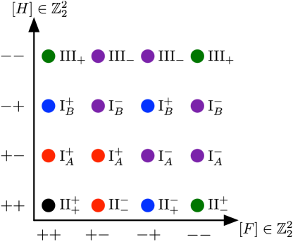
Refer to caption
Figure 33: Discrete torsion for all phases of the dP1𝑑subscript𝑃1dP_{1} orientifold. Except for the relative position of III+ and III-, all torsions are fixed by the partial resolution to the 3/3superscript3subscript3\mathbb{C}^{3}/\mathbb{Z}_{3} orientifold singularity plus an O3 plane. The [F]delimited-[]𝐹[F] torsion assignment for phase III is obtained by matching discrete symmetries between prospective S-duals.

5.1 Matching the superconformal index

With an extensive set of predicted S-dualities in hand, we need a way to test these dualities. Anomaly matching is not sensitive enough, because all the theories with the same D3 charge (47) have matching anomalies regardless of [F]delimited-[]𝐹[F] and [H]delimited-[]𝐻[H] torsion, apart from the mismatch of the SU(2)3𝑆𝑈superscript23SU(2)^{3} Witten anomalies between IA+superscriptsubscriptI𝐴\mathrm{I}_{A}^{+} and IB+superscriptsubscriptI𝐵\mathrm{I}_{B}^{+} noted in dualities1 , which persists in their duals.313131We have not computed the Witten anomaly or the SU(2)22𝑆𝑈superscript22subscript2SU(2)^{2}\mathbb{Z}_{2} anomaly in phase III, where only U(1)XSU(2)𝑈subscript1𝑋𝑆𝑈2U(1)_{X}\subset SU(2) is manifest. Based on the 2subscript2\mathbb{Z}_{2} discrete symmetry discussed above and on the quantization condition for U(1)B𝑈subscript1𝐵U(1)_{B} (which is integral for IA/Bsuperscriptsubscriptabsent𝐴𝐵{}_{A/B}^{-}, III±, and II+subscriptsuperscriptabsent{}^{+}_{-}, and otherwise half-integral), we can rule out any further dualities between the dP1𝑑subscript𝑃1dP_{1} theories besides those in (46).

To do better, we could match the operator spectra of the dual theories. This can be subtle due to the large number of gauge invariant operators in a quiver gauge theory, quantum constraints on the moduli space, etc., and we leave a more extensive treatment to future work. Instead, we rely on a conceptually simple but very sensitive test: we match the superconformal indices between the dual theories.

The superconformal index Romelsberger:2005eg ; Kinney:2005ej counts shortened superconformal multiplets of the theory quantized on S3×superscript𝑆3S^{3}\times\mathbb{R} up to recombination:

=Tr=0[(1)FtR+2JLx2JRf],subscriptTr0superscript1𝐹superscript𝑡𝑅2subscript𝐽𝐿superscript𝑥2subscript𝐽𝑅𝑓\mathcal{I}=\operatorname{Tr}_{\mathcal{H}=0}\left[(-1)^{F}t^{R+2J_{L}}x^{2J_{R}}f\right]\,, (48)

where JL,Rsubscript𝐽𝐿𝑅J_{L,R} generate the Cartan of SU(2)L,R𝑆𝑈subscript2𝐿𝑅SU(2)_{L,R}, R𝑅R denotes the R-charge, and f𝑓f is an arbitrary fugacity of the flavor symmetry group. The trace is taken over states annihilated by

H2JL32R,𝐻2subscript𝐽𝐿32𝑅\mathcal{H}\equiv H-2J_{L}-\frac{3}{2}R\,, (49)

with H𝐻H the Hamiltonian, which is the anticommutator of a supercharge Q𝑄Q in the superconformal algebra with its conjugate (hence the index is counts Q𝑄Q cohomology classes.)

The superconformal index can be shown to agree between Seiberg dual theories Romelsberger:2007ec , where it reduces to an integral identity for elliptic hypergeometric functions Dolan:2008qi . In the case of other dualities, such as S-dualities, the index should likewise agree, but the appropriate integral identities are not always known, see e.g. Spiridonov:2009za ; Spiridonov:2010qv .

The index is invariant under continuous deformations Romelsberger:2007ec , so in particular when a weakly-coupled UV description is available — and in the absence of rank-enhancing accidental symmetries along the flow — the index can be computed in the UV. We have

=𝑑gPE[aia(t,x,g,f)],differential-d𝑔𝑃𝐸delimited-[]subscript𝑎subscript𝑖𝑎𝑡𝑥𝑔𝑓\mathcal{I}=\int dg\,P\!E\!\left[\sum_{a}i_{a}(t,x,g,f)\right]\,, (50)

where PE[f(x)]exp(k=11kf(xk))𝑃𝐸delimited-[]𝑓𝑥superscriptsubscript𝑘11𝑘𝑓superscript𝑥𝑘P\!E[f(x)]\equiv\exp\left(\sum_{k=1}^{\infty}\frac{1}{k}f(x^{k})\right) is the plethystic exponential, the integral is taken over the gauge group with the Haar measure, and iasubscript𝑖𝑎i_{a} is the “letter” for the a𝑎ath field, of the form

iV=2t2t(x+x1)(1tx)(1tx1)χV,iΦ=tRχΦt2RχΦ(1tx)(1tx1),formulae-sequencesubscript𝑖𝑉2superscript𝑡2𝑡𝑥superscript𝑥11𝑡𝑥1𝑡superscript𝑥1subscript𝜒𝑉subscript𝑖Φsuperscript𝑡𝑅subscript𝜒Φsuperscript𝑡2𝑅subscript𝜒superscriptΦ1𝑡𝑥1𝑡superscript𝑥1i_{V}=\frac{2t^{2}-t(x+x^{-1})}{(1-tx)(1-tx^{-1})}\chi_{V}\;\;,\;\;i_{\Phi}=\frac{t^{R}\chi_{\Phi}-t^{2-R}\chi_{\Phi^{\dagger}}}{(1-tx)(1-tx^{-1})}\,, (51)

for vector and chiral superfields, respectively. Here R𝑅R is the a𝑎a-maximized R-charge of the chiral field and χVsubscript𝜒𝑉\chi_{V} and χΦsubscript𝜒Φ\chi_{\Phi} denote the group characters of the representation under the gauge and global symmetries. In effect, (50) counts gauge-invariants in the symmetric product of the states in the letter, where negative contributions to the letter anticommute.

In general, the integral over the gauge group is very difficult to perform, except at large N𝑁N, where it simplifies Kinney:2005ej . Instead, we perform a series expansion in t𝑡t to count low-lying states in the index. Using

𝑑gχr(g)=δr,1,χr(g)χr(g)=χr×r(g),formulae-sequencedifferential-d𝑔subscript𝜒𝑟𝑔subscript𝛿𝑟1subscript𝜒𝑟𝑔subscript𝜒superscript𝑟𝑔subscript𝜒𝑟superscript𝑟𝑔\int dg\,\chi_{r}(g)=\delta_{r,1}\;\;,\;\;\chi_{r}(g)\chi_{r^{\prime}}(g)=\chi_{r\times r^{\prime}}(g)\,, (52)

for representations r,r𝑟superscript𝑟r,r^{\prime}, where δr,1subscript𝛿𝑟1\delta_{r,1} denotes the number of singlet irreps in r𝑟r, it becomes straightforward in principle to compute the index to any fixed order in t𝑡t, provided that all the chiral fields satisfy 0<R<20𝑅20<R<2.

Unfortunately, the a𝑎a-maximized R-charges of the fundamental fields in the UV theory need not satisfy this inequality, even in the absence of accidental symmetries which mix with the R-symmetry in the infrared. For instance, the deconfined description of an SU(N)𝑆𝑈𝑁SU(N) antisymmetric tensor, figure 20, has the a𝑎a-maximized R-charges:

R(Z^)=13,R(P)=N63F,R(Q)=53+N63F,R(T)=2+2N63F,formulae-sequence𝑅^𝑍13formulae-sequence𝑅𝑃𝑁63𝐹formulae-sequence𝑅𝑄53𝑁63𝐹𝑅𝑇22𝑁63𝐹R(\hat{Z})=\frac{1}{3}\;\;,\;\;R(P)=-\frac{N-6}{3F}\;\;,\;\;R(Q)=\frac{5}{3}+\frac{N-6}{3F}\;\;,\;\;R(T)=2+2\frac{N-6}{3F}\,, (53)

where F𝐹F is the number of flavors in the deconfined description, with (1)F=(1)Nsuperscript1𝐹superscript1𝑁(-1)^{F}=(-1)^{N}. These charges satisfy the bound 0<R<20𝑅20<R<2 for N<6𝑁6N<6 and violate it otherwise, whereas in either case the infrared fixed point consists of free chiral multiplets with R-charge 2/3232/3, by construction.

The resolution is that the states with negative powers of t𝑡t completely cancel out of the index. To see how this work, consider the marginal case N=6𝑁6N=6 in the above deconfined theory, so that R(P)=R(T¯)=0𝑅𝑃𝑅¯𝑇0R(P)=R(\bar{T})=0, where T¯¯𝑇\bar{T} denotes the negative contribution to the letter for T𝑇T. Naively, there are an infinite number of contributions to the index at 𝒪(t0)𝒪superscript𝑡0\mathcal{O}(t^{0}). However, it is straightforward to check that integrating over the symplectic group gives:

𝑑gPE[yχ (g)χ¯ (f)]=PE[y2χ¯ (f)],differential-d𝑔𝑃𝐸delimited-[]𝑦subscript𝜒 𝑔subscript𝜒¯absent 𝑓𝑃𝐸delimited-[]superscript𝑦2subscript𝜒¯absent 𝑓\int dg\,P\!E[y\chi_{\leavevmode\hbox{$\vbox{\hbox{\vtop{ \offinterlineskip\openup-0.27995pt\halign{&\opttoksa@YT={\font@YT}\getcolor@YT{\save@YT{\opttoksb@YT}}\nil@YT\getcolor@YT{\startbox@@YT\the\opttoksa@YT\the\opttoksb@YT}#\endbox@YT\cr\lower 0.27995pt\vbox{\kern 0.00002pt\kern 0.13997pt\hbox{\kern 0.27995pt\vbox to3.77995pt{\vss\hbox to3.5pt{\hss$$\hss}\vss}\kern-3.77995pt\vrule height=3.77995pt,width=0.27995pt\kern 3.5pt\vrule height=3.77995pt,width=0.27995pt}\kern-0.13997pt\kern-3.77995pt\hrule width=4.0599pt,height=0.27995pt\kern 3.5pt\hrule width=4.0599pt,height=0.27995pt}\cr}}\kern 4.4599pt}}$}}(g)\chi_{\overline{}\leavevmode\hbox{$\vbox{\hbox{\vtop{ \offinterlineskip\openup-0.27995pt\halign{&\opttoksa@YT={\font@YT}\getcolor@YT{\save@YT{\opttoksb@YT}}\nil@YT\getcolor@YT{\startbox@@YT\the\opttoksa@YT\the\opttoksb@YT}#\endbox@YT\cr\lower 0.27995pt\vbox{\kern 0.00002pt\kern 0.13997pt\hbox{\kern 0.27995pt\vbox to3.77995pt{\vss\hbox to3.5pt{\hss$$\hss}\vss}\kern-3.77995pt\vrule height=3.77995pt,width=0.27995pt\kern 3.5pt\vrule height=3.77995pt,width=0.27995pt}\kern-0.13997pt\kern-3.77995pt\hrule width=4.0599pt,height=0.27995pt\kern 3.5pt\hrule width=4.0599pt,height=0.27995pt}\cr}}\kern 4.4599pt}}$}}(f)]=P\!E\!\left[y^{2}\chi_{\overline{}\leavevmode\hbox{$\vbox{\hbox{\vtop{ \offinterlineskip\openup-0.27995pt\halign{&\opttoksa@YT={\font@YT}\getcolor@YT{\save@YT{\opttoksb@YT}}\nil@YT\getcolor@YT{\startbox@@YT\the\opttoksa@YT\the\opttoksb@YT}#\endbox@YT\cr\lower 0.27995pt\vbox{\kern 0.00002pt\kern 0.13997pt\hbox{\kern 0.27995pt\vbox to3.77995pt{\vss\hbox to3.5pt{\hss$$\hss}\vss}\kern-3.77995pt\vrule height=3.77995pt,width=0.27995pt\kern 3.5pt\vrule height=3.77995pt,width=0.27995pt}\kern-0.13997pt\kern-3.77995pt\hrule width=4.0599pt,height=0.27995pt\kern 3.5pt\hrule width=4.0599pt,height=0.27995pt}\cr\lower 0.27995pt\vbox{\kern 0.00002pt\kern 0.13997pt\hbox{\kern 0.27995pt\vbox to3.77995pt{\vss\hbox to3.5pt{\hss$$\hss}\vss}\kern-3.77995pt\vrule height=3.77995pt,width=0.27995pt\kern 3.5pt\vrule height=3.77995pt,width=0.27995pt}\kern-0.13997pt\kern-3.77995pt\hrule width=4.0599pt,height=0.27995pt\kern 3.5pt\hrule width=4.0599pt,height=0.27995pt}\cr}}\kern 4.4599pt}}$}}(f)\right]\,, (54)

i.e. the gauge invariant operator P2ksuperscript𝑃2𝑘P^{2k} transforms in k𝑘kth symmetric power of the conjugate antisymmetric representation of SU(F)𝑆𝑈𝐹SU(F), so that the contributions of P2ksuperscript𝑃2𝑘P^{2k} and T¯ksuperscript¯𝑇𝑘\bar{T}^{k} to the 𝒪(t0)𝒪superscript𝑡0\mathcal{O}(t^{0}) term in the index cancel.

In fact, this cancellation is guaranteed by the integral identities of Dolan:2008qi , since the reconfinement of the deconfined description is a special case of Seiberg duality for symplectic groups, but it serves to illustrate the difficulties which arise in computing the index in more general theories whose fundamental fields do not satisfy 0<R<20𝑅20<R<2.

The a𝑎a-maximized R-charge for tables 2, 3, 6, 7 is

U(1)R(sc)=U(1)R+(4β)U(1)Y+QD3(3ββ4)U(1)B𝑈superscriptsubscript1𝑅sc𝑈subscript1𝑅4𝛽𝑈subscript1𝑌subscript𝑄D33𝛽𝛽4𝑈subscript1𝐵U(1)_{R}^{\rm(sc)}=U(1)_{R}+(4-\beta)\,U(1)_{Y}+Q_{\rm D3}\left(\frac{3}{\beta}-\frac{\beta}{4}\right)U(1)_{B} (55)

where QD3subscript𝑄D3Q_{\rm D3} is given by (47), and β𝛽\beta is the unique root of the quartic equation

(β2)(β6)(3β28β12)QD32+16β2(92β)=0𝛽2𝛽63superscript𝛽28𝛽12superscriptsubscript𝑄D3216superscript𝛽292𝛽0(\beta-2)(\beta-6)(3\beta^{2}-8\beta-12)Q_{\rm D3}^{2}+16\beta^{2}(9-2\beta)=0 (56)

satisfying 23(2+13)<β423213𝛽4\frac{2}{3}\left(2+\sqrt{13}\right)<\beta\leq 4 for QD34subscript𝑄D34Q_{\rm D3}\geq 4, with 23(2+13)3.737232133.737\frac{2}{3}\left(2+\sqrt{13}\right)\approx 3.737. From this, one can check that the a𝑎a-maximized R-charges in tables 2, 3 satisfy 0<R<20𝑅20<R<2 for QD3>4subscript𝑄D34Q_{\rm D3}>4,323232QD3=4subscript𝑄D34Q_{\rm D3}=4 is a special case where there is confinement with chiral symmetry breaking in the infrared dualities1 . whereas those in table 6 satisfy the constraint for 4<QD3134subscript𝑄D3134<Q_{\rm D3}\leq 13 with F=1𝐹1F=1 and for 4<QD3124subscript𝑄D3124<Q_{\rm D3}\leq 12 with F=2𝐹2F=2, and those in table 7 satisfy it for 4<QD3104subscript𝑄D3104<Q_{\rm D3}\leq 10 with F=1,2𝐹12F=1,2.

For the present paper, we confine out attention to 4<QD3104subscript𝑄D3104<Q_{\rm D3}\leq 10, for which the index can be computed as an expansion in t𝑡t in all the phases of dP1𝑑subscript𝑃1dP_{1}.333333Besides finding a systematic way to deal with the large degree of cancellation in the index, another way to proceed for QD3>10subscript𝑄D310Q_{\rm D3}>10 would be to expand in a different fugacity. One can show that there is always a conserved R-symmetry (not necessarily the a𝑎a-maximized one) satisfying 0<R<20𝑅20<R<2 for any QD3>4subscript𝑄D34Q_{\rm D3}>4 and F>0𝐹0F>0, hence there is a corresponding fugacity with only positive powers in the letter, allowing a systematic expansion which avoids the above issues. This already allows for very non-trivial tests of the duality.

Consider for example QD3=9subscript𝑄D39Q_{\rm D3}=9. The superconformal index in phase I+Asuperscriptsubscriptabsent𝐴{}_{A}^{+} is:

1+b12y5t(1.294)17+272β+31β8+b12y4X1t(1.488)13+272β+23β8+b12y3X2t(1.683)9+272β+15β8+b12y2X3t(1.877)5+272β+7β8(1+X2)t2++[J1(3+7X2+4X4)2J3(1+X2)]t5+1superscript𝑏12superscript𝑦5superscriptsubscript𝑡(1.294)17272𝛽31𝛽8superscript𝑏12superscript𝑦4subscript𝑋1superscriptsubscript𝑡(1.488)13272𝛽23𝛽8superscript𝑏12superscript𝑦3subscript𝑋2superscriptsubscript𝑡(1.683)9272𝛽15𝛽8superscript𝑏12superscript𝑦2subscript𝑋3superscriptsubscript𝑡(1.877)5272𝛽7𝛽81subscript𝑋2superscript𝑡2delimited-[]subscript𝐽137subscript𝑋24subscript𝑋42subscript𝐽31subscript𝑋2superscript𝑡51+b^{{\frac{1}{2}}}y^{{-5}}t_{\text{(1.294)}}^{{-17+\frac{27}{2\beta}+\frac{31\beta}{8}}}+b^{{\frac{1}{2}}}y^{{-4}}X_{1}t_{\text{(1.488)}}^{{-13+\frac{27}{2\beta}+\frac{23\beta}{8}}}+b^{{\frac{1}{2}}}y^{{-3}}X_{2}t_{\text{(1.683)}}^{{-9+\frac{27}{2\beta}+\frac{15\beta}{8}}}+b^{{\frac{1}{2}}}y^{{-2}}X_{3}t_{\text{(1.877)}}^{{-5+\frac{27}{2\beta}+\frac{7\beta}{8}}}\\ -\left(1+X_{2}\right)t^{2}+\ldots+\left[J_{1}\left(3+7X_{2}+4X_{4}\right)-2J_{3}\left(1+X_{2}\right)\right]t^{5}+\ldots (57)

up to order t5superscript𝑡5t^{5}, where y𝑦y and b𝑏b are the flavor fugacities for U(1)Y𝑈subscript1𝑌U(1)_{Y} and U(1)B𝑈subscript1𝐵U(1)_{B}, respectively, and Xisubscript𝑋𝑖X_{i} and Jisubscript𝐽𝑖J_{i} denote the characters for the spin i/2𝑖2i/2 representation of the SU(2)𝑆𝑈2SU(2) flavor symmetry and of SU(2)R𝑆𝑈subscript2𝑅SU(2)_{R}, respectively. In cases where t𝑡t is raised to an irrational exponent, we indicate a decimal approximant in the subscript. Note that we have shown only the first and last few terms in the expansion (57). The full expression, shown in §C.3, has 180 terms, of which only 12 have been given above!

The index for I+Bsuperscriptsubscriptabsent𝐵{}_{B}^{+} and QD3=9subscript𝑄D39Q_{\rm D3}=9 is

1+b32y4t(1.021)12+812β+5β8(1+X2)t2+b32y4J1t(2.021)11+812β+5β8+b3y8t(2.041)24+81β+5β4yX1t(2.194)6β+b12X4t(2.734)2272β+9β8++[J1(3+7X2+4X4)2J3(1+X2)]t5+1superscript𝑏32superscript𝑦4superscriptsubscript𝑡(1.021)12812𝛽5𝛽81subscript𝑋2superscript𝑡2superscript𝑏32superscript𝑦4subscript𝐽1superscriptsubscript𝑡(2.021)11812𝛽5𝛽8superscript𝑏3superscript𝑦8superscriptsubscript𝑡(2.041)2481𝛽5𝛽4𝑦subscript𝑋1superscriptsubscript𝑡(2.194)6𝛽superscript𝑏12subscript𝑋4superscriptsubscript𝑡(2.734)2272𝛽9𝛽8delimited-[]subscript𝐽137subscript𝑋24subscript𝑋42subscript𝐽31subscript𝑋2superscript𝑡51+b^{{\frac{3}{2}}}y^{{-4}}t_{\text{(1.021)}}^{{-12+\frac{81}{2\beta}+\frac{5\beta}{8}}}-\left(1+X_{2}\right)t^{2}+b^{{\frac{3}{2}}}y^{{-4}}J_{1}t_{\text{(2.021)}}^{{-11+\frac{81}{2\beta}+\frac{5\beta}{8}}}+b^{3}y^{{-8}}t_{\text{(2.041)}}^{{-24+\frac{81}{\beta}+\frac{5\beta}{4}}}-yX_{1}t_{\text{(2.194)}}^{{6-\beta}}\\ +b^{{-\frac{1}{2}}}X_{4}t_{\text{(2.734)}}^{{2-\frac{27}{2\beta}+\frac{9\beta}{8}}}+\ldots+\left[J_{1}\left(3+7X_{2}+4X_{4}\right)-2J_{3}\left(1+X_{2}\right)\right]t^{5}+\ldots (58)

up to order t5superscript𝑡5t^{5}, where the full expression, shown in §C.4, has 154 terms. We see immediately that (57) and (58) do not match, hence I+Asuperscriptsubscriptabsent𝐴{}_{A}^{+} and I+Bsuperscriptsubscriptabsent𝐵{}_{B}^{+} are not dual, as anticipated in dualities1 and borne out by figure 33. By contrast, computing the index for IIsubscriptsuperscriptabsent{}^{-}_{-} to the same order gives back all 180 terms of (57), and computing the index for II+subscriptsuperscriptabsent{}^{-}_{+} gives back all 154 terms of (58)! This is highly non-trivial evidence in favor of the dualities IA+IIsuperscriptsubscriptI𝐴subscriptsuperscriptII\mathrm{I}_{A}^{+}\longleftrightarrow\mathrm{II}^{-}_{-} and IB+II+superscriptsubscriptI𝐵subscriptsuperscriptII\mathrm{I}_{B}^{+}\longleftrightarrow\mathrm{II}^{-}_{+}.

Likewise, the index for IAsuperscriptsubscriptabsent𝐴{}_{A}^{-} and QD3=8subscript𝑄D38Q_{\rm D3}=8 is

1(1+X2)t2yX1t(2.178)6β+by7t(2.39)23+24β+5β+by6X1t(2.568)19+24β+4β+2by5X2t(2.746)15+24β+3β++[9+10X2+3X42X6+2J2(3+8X2+3X4)2J4(1+X2)]t6+11subscript𝑋2superscript𝑡2𝑦subscript𝑋1superscriptsubscript𝑡(2.178)6𝛽𝑏superscript𝑦7superscriptsubscript𝑡(2.39)2324𝛽5𝛽𝑏superscript𝑦6subscript𝑋1superscriptsubscript𝑡(2.568)1924𝛽4𝛽2𝑏superscript𝑦5subscript𝑋2superscriptsubscript𝑡(2.746)1524𝛽3𝛽delimited-[]910subscript𝑋23subscript𝑋42subscript𝑋62subscript𝐽238subscript𝑋23subscript𝑋42subscript𝐽41subscript𝑋2superscript𝑡61-(1+X_{2})t^{2}-yX_{1}t_{\text{(2.178)}}^{6-\beta}+by^{{-7}}t_{\text{(2.39)}}^{{-23+\frac{24}{\beta}+5\beta}}+by^{{-6}}X_{1}t_{\text{(2.568)}}^{{-19+\frac{24}{\beta}+4\beta}}+2by^{{-5}}X_{2}t_{\text{(2.746)}}^{{-15+\frac{24}{\beta}+3\beta}}\\ +\ldots+\left[9+10X_{2}+3X_{4}-2X_{6}+2J_{2}\left(3+8X_{2}+3X_{4}\right)-2J_{4}\left(1+X_{2}\right)\right]t^{6}+\ldots (59)

up to order t6superscript𝑡6t^{6}. The full result in §C.2 has 215 terms, all of which are reproduced in both IBsuperscriptsubscriptabsent𝐵{}_{B}^{-} and III-! This is highly non-trivial evidence for the duality IAIBsuperscriptsubscriptI𝐴superscriptsubscriptI𝐵\mathrm{I}_{A}^{-}\longleftrightarrow\mathrm{I}_{B}^{-} proposed in dualities1 , now expanded into a triality IAIBIIIsuperscriptsubscriptI𝐴superscriptsubscriptI𝐵subscriptIII\mathrm{I}_{A}^{-}\longleftrightarrow\mathrm{I}_{B}^{-}\longleftrightarrow\mathrm{III}_{-}.

Finally, the index for II+subscriptsuperscriptabsent{}^{+}_{-} and QD3=8subscript𝑄D38Q_{\rm D3}=8 is343434We omit the fugacity for the 2subscript2\mathbb{Z}_{2} discrete symmetry for simplicity.

1+b1y4X5t(1.077)1524β2β(1+X2)t2+b1y4J1X5t(2.077)1624β2β+b2y8(X2+X6+X10)t(2.153)3048β4βyt(2.178)6βX1++[J1(5+14X2+12X4+7X6+4X8)2J3(1+X2)]t5+1superscript𝑏1superscript𝑦4subscript𝑋5superscriptsubscript𝑡(1.077)1524𝛽2𝛽1subscript𝑋2superscript𝑡2superscript𝑏1superscript𝑦4subscript𝐽1subscript𝑋5superscriptsubscript𝑡(2.077)1624𝛽2𝛽superscript𝑏2superscript𝑦8subscript𝑋2subscript𝑋6subscript𝑋10superscriptsubscript𝑡(2.153)3048𝛽4𝛽𝑦superscriptsubscript𝑡(2.178)6𝛽subscript𝑋1delimited-[]subscript𝐽1514subscript𝑋212subscript𝑋47subscript𝑋64subscript𝑋82subscript𝐽31subscript𝑋2superscript𝑡51+b^{{-1}}y^{4}X_{5}t_{\text{(1.077)}}^{{15-\frac{24}{\beta}-2\beta}}-\left(1+X_{2}\right)t^{2}+b^{{-1}}y^{4}J_{1}X_{5}t_{\text{(2.077)}}^{{16-\frac{24}{\beta}-2\beta}}+b^{{-2}}y^{8}\left(X_{2}+X_{6}+X_{10}\right)t_{\text{(2.153)}}^{{30-\frac{48}{\beta}-4\beta}}\\ -yt_{\text{(2.178)}}^{{6-\beta}}X_{1}+\ldots+\left[J_{1}\left(5+14X_{2}+12X_{4}+7X_{6}+4X_{8}\right)-2J_{3}\left(1+X_{2}\right)\right]t^{5}+\ldots (60)

up to order t5superscript𝑡5t^{5}, where the full result in §C.1 has 216 terms, all of which are reproduced in III+! This confirms the last remaining duality II+III+subscriptsuperscriptIIsubscriptIII\mathrm{II}^{+}_{-}\longleftrightarrow\mathrm{III}_{+} from figure 33.

For completeness, we also give the first few terms of the index for II++subscriptsuperscriptabsent{}^{+}_{+} and QD3=8subscript𝑄D38Q_{\rm D3}=8:

1+b3/2t(0.830)212+36β+β2y7/2+bt(1.017)312+12β+7β2y9/2+y4X5t(1.077)1524β2βb+bX1t(1.195)232+12β+5β2y7/2+bX2t(1.373)152+12β+3β2y5/2+bX3t(1.551)72+12β+β2y3/2+b3t(1.660)21+72β+βy7+bX4t(1.729)12+12ββ2y+1superscript𝑏32superscriptsubscript𝑡0.83021236𝛽𝛽2superscript𝑦72𝑏superscriptsubscript𝑡1.01731212𝛽7𝛽2superscript𝑦92superscript𝑦4subscript𝑋5superscriptsubscript𝑡1.0771524𝛽2𝛽𝑏𝑏subscript𝑋1superscriptsubscript𝑡1.19523212𝛽5𝛽2superscript𝑦72𝑏subscript𝑋2superscriptsubscript𝑡1.37315212𝛽3𝛽2superscript𝑦52𝑏subscript𝑋3superscriptsubscript𝑡1.5517212𝛽𝛽2superscript𝑦32superscript𝑏3superscriptsubscript𝑡1.6602172𝛽𝛽superscript𝑦7𝑏subscript𝑋4superscriptsubscript𝑡1.7291212𝛽𝛽2𝑦1+\frac{b^{3/2}t_{(0.830)}^{-\frac{21}{2}+\frac{36}{\beta}+\frac{\beta}{2}}}{y^{7/2}}+\frac{\sqrt{b}t_{(1.017)}^{-\frac{31}{2}+\frac{12}{\beta}+\frac{7\beta}{2}}}{y^{9/2}}+\frac{y^{4}X_{5}t_{(1.077)}^{15-\frac{24}{\beta}-2\beta}}{b}+\frac{\sqrt{b}X_{1}t_{(1.195)}^{-\frac{23}{2}+\frac{12}{\beta}+\frac{5\beta}{2}}}{y^{7/2}}\\ +\frac{\sqrt{b}X_{2}t_{(1.373)}^{-\frac{15}{2}+\frac{12}{\beta}+\frac{3\beta}{2}}}{y^{5/2}}+\frac{\sqrt{b}X_{3}t_{(1.551)}^{-\frac{7}{2}+\frac{12}{\beta}+\frac{\beta}{2}}}{y^{3/2}}+\frac{b^{3}t_{(1.660)}^{-21+\frac{72}{\beta}+\beta}}{y^{7}}+\frac{\sqrt{b}X_{4}t_{(1.729)}^{\frac{1}{2}+\frac{12}{\beta}-\frac{\beta}{2}}}{\sqrt{y}}+\ldots (61)

Notice that (61) does not match (59) or (60), just as (57) and (58) do not match, even for the first few terms. Thus, the superconformal index is a highly sensitive test of S-dualities. The S-dual theories in figure 33 have indices which match hundreds of terms (and conjecturally exactly), whereas the dP1𝑑subscript𝑃1dP_{1} theories which are not S-dual have indices which disagree even in the first few terms!353535To be precise, the leading baryons generally disagree. For larger values of QD3subscript𝑄D3Q_{\rm D3}, these baryons will appear with higher powers of t𝑡t and the leading 𝒪(b0)𝒪superscript𝑏0\mathcal{O}(b^{0}) terms will match, even between non-S-dual theories, as the index approaches a large N𝑁N limit.

We have also matched the superconformal indices between the dual theories for other values of QD310subscript𝑄D310Q_{\rm D3}\leq 10. Our results are summarized in table 8.

QD3subscript𝑄D3Q_{\rm D3} IA+=IIsuperscriptsubscriptI𝐴subscriptsuperscriptII\mathrm{I}_{A}^{+}=\mathrm{II}^{-}_{-} IB+=II+superscriptsubscriptI𝐵subscriptsuperscriptII\mathrm{I}_{B}^{+}=\mathrm{II}^{-}_{+}
Terms Order Terms Order
5 *275 𝒪(t2)𝒪superscript𝑡2\mathcal{O}(t^{2}) *222 𝒪(t2)𝒪superscript𝑡2\mathcal{O}(t^{2})
7 221 𝒪(t4)𝒪superscript𝑡4\mathcal{O}(t^{4}) *187 𝒪(t4)𝒪superscript𝑡4\mathcal{O}(t^{4})
9 180 𝒪(t5)𝒪superscript𝑡5\mathcal{O}(t^{5}) 154 𝒪(t5)𝒪superscript𝑡5\mathcal{O}(t^{5})
QD3subscript𝑄D3Q_{\rm D3} IA=IB=IIIsuperscriptsubscriptI𝐴superscriptsubscriptI𝐵subscriptIII\mathrm{I}_{A}^{-}=\mathrm{I}_{B}^{-}=\mathrm{III}_{-} II+=III+subscriptsuperscriptIIsubscriptIII\mathrm{II}^{+}_{-}=\mathrm{III}_{+}
Terms Order Terms Order
6 145 𝒪(t4)𝒪superscript𝑡4\mathcal{O}(t^{4}) *135 𝒪(t3)𝒪superscript𝑡3\mathcal{O}(t^{3})
8 215 𝒪(t6)𝒪superscript𝑡6\mathcal{O}(t^{6}) 216 𝒪(t5)𝒪superscript𝑡5\mathcal{O}(t^{5})
10 110 𝒪(t6)𝒪superscript𝑡6\mathcal{O}(t^{6}) 1 𝒪(t5/4)𝒪superscript𝑡54\mathcal{O}(t^{5/4})
Table 8: Summary of S-duality checks using the superconformal index. For III+subscriptIII\mathrm{III}_{+} and QD3=10subscript𝑄D310Q_{\rm D3}=10, we are unable to compute any non-vanishing terms in the index beyond the leading 111, but can show that several contributions cancel as required to match the S-dual theory. The starred theories have accidental symmetries, but the index still matches for the manifest flavor symmetries.

6 Conclusions

In this paper we have argued that in studying 𝒩=1𝒩1\mathcal{N}=1 S-duality in Calabi-Yau orientifolds, as initiated in dualities1 ; Bianchi:2013gka ; dualities2 , one is forced to include strongly-coupled sectors. In toric examples, these sectors arise from more than two NS5 branes intersecting atop an O5 plane on a D5 brane stack, such as the quad CFTs described in §3.3 and constructed in §4.

In the cases we have studied, these sectors have simple yet non-trivial properties. They are characterized by a large flavor symmetry group and a moduli space with mesonic and baryonic directions, where the mesonic directions relate CFTs with different ranks, and the baryonic directions relate the CFT to weakly-coupled chiral superfields describing brane recombinations which avoid the higher-multiplicity intersection. A remarkable property of these CFTs is the appearance of spinor representations of the SO(2(M+4))𝑆𝑂2𝑀4SO(2(M+4)) flavor symmetry in the baryonic spectrum for arbitrary M𝑀M. This property is hidden in the deconfined gauge theory description, and indeed it is difficult to imagine how it could have been manifest, since the dimension of the spinor representation grows exponentially with M𝑀M, in conflict with asymptotic freedom. This confirms the intrinsically strongly-coupled (non-Lagrangian) nature of the quad CFTs.

By coupling these quad CFTs to quiver gauge theories, as dictated by the brane tiling construction, we have obtained a complete picture of S-dualities in the dP1𝑑subscript𝑃1dP_{1} orientifold considered in this paper. Our description has been subjected to stringent consistency checks using one of the best instruments available in minimally supersymmetric theories, the superconformal index. We expect that similar ingredients can be used to understand S-duality in a broad class of toric orientifolds toricII , if not beyond.

The quad CFTs — and similar strongly-coupled sectors arising from 2k2𝑘2k NS5 branes intersecting atop an O5 plane with k>2𝑘2k>2 — are interesting in their own right, and deserve further study. It would be instructive to determine the string-theory origin of the non-abelian enhancement to USp(2M)𝑈𝑆𝑝2𝑀U\!Sp(2M) or SO(2(M+4))𝑆𝑂2𝑀4SO(2(M+4)), and in particular the appearance of spinor representations in the latter case. Other descriptions of these CFTs, such as by symmetric tensor deconfinement, could be developed further. The superconformal index of these CFTs may admit a description which is independent of the deconfinement procedure, making their properties and symmetries manifest. It would also be interesting to determine whether these same CFTs play a role in orientifolds of non-toric Calabi-Yau singularities.

Recently, there has been some progress in describing certain S-dualities of chiral 𝒩=1𝒩1\mathcal{N}=1 theories in terms of a 6d (1,0)10(1,0) theory compactified on a punctured Riemann surface Gaiotto:2015usa ; Franco:2015jna ; Hanany:2015pfa . It remains to be seen if our S-dualities fall into this class, in which case they might form part of a yet-unknown unified picture of 𝒩=1𝒩1\mathcal{N}=1 dualities.

Finally, while our discussion has focused on the brane tiling in the gssubscript𝑔𝑠g_{s}\to\infty limit, it should be possible to describe the new phases in the gs0subscript𝑔𝑠0g_{s}\to 0 limit as well as in the mirror description with intersecting D6 branes. At present, this is an open problem.

Acknowledgements.
We thank A. Hanany for discussions, and T. Wrase for collaboration in related previous work dualities1 ; dualities2 . BH is supported by the Fundamental Laws Initiative of the Harvard Center for the Fundamental Laws of Nature. I. G.-E. thanks N. Hasegawa for kind encouragement and constant support.

Appendix A Del Pezzo orientifold singularities

In this appendix, we construct the ten del Pezzo singularities and their orientifolds with the del Pezzo as an isolated fixed plane.363636Embeddings for the non-toric del Pezzo singularities are taken from Malyshev:2007yb and references therein.

The del Pezzo singularities for dPk𝑑subscript𝑃𝑘dP_{k}, k5𝑘5k\geq 5, are complete intersection singularities. Let Pr(a1,,ap)superscriptsubscript𝑃𝑟subscript𝑎1subscript𝑎𝑝P_{r}^{(a_{1},\ldots,a_{p})} denote a generic quasi-homogeneous polynomial of weight r𝑟r in p𝑝p variables with weights (a1,,ap)subscript𝑎1subscript𝑎𝑝(a_{1},\ldots,a_{p}). The dP6𝑑subscript𝑃6dP_{6}, dP7𝑑subscript𝑃7dP_{7}, and dP8𝑑subscript𝑃8dP_{8} singularities are the hypersurfaces P3(1,1,1,1)=0superscriptsubscript𝑃311110P_{3}^{(1,1,1,1)}=0, P4(1,1,1,2)=0superscriptsubscript𝑃411120P_{4}^{(1,1,1,2)}=0 and P6(1,1,2,3)=0superscriptsubscript𝑃611230P_{6}^{(1,1,2,3)}=0 in 4superscript4\mathbb{C}^{4}, respectively, whereas the dP5𝑑subscript𝑃5dP_{5} singularity is the complete intersection of two quadrics P2(1,1)=R2(1,1)=0superscriptsubscript𝑃211superscriptsubscript𝑅2110P_{2}^{(1,1)}=R_{2}^{(1,1)}=0 in 5superscript5\mathbb{C}^{5}. In each case, the involution σ𝜎\sigma reflects the odd-weight coordinates and leaves the even-weight coordinates invariant.

The del Pezzo surfaces dPk𝑑subscript𝑃𝑘dP_{k} for k3𝑘3k\leq 3 and 𝔽0subscript𝔽0\mathbb{F}_{0} are toric, as are the corresponding singularities. These singularities are most easily described as the classical moduli space of a gauged linear sigma model (GLSM) with vanishing Fayet-Iliopoulos (FI) parameters:

dP0𝑑subscript𝑃0\displaystyle dP_{0} :xyz3ω3ω3ω3,:absentmissing-subexpression𝑥𝑦𝑧missing-subexpressionmissing-subexpressionmissing-subexpressionmissing-subexpressionsubscript3subscript𝜔3subscript𝜔3subscript𝜔3\displaystyle:\begin{array}[]{c|ccc}&x&y&z\\ \hline\cr\mathbb{Z}_{3}&\omega_{3}&\omega_{3}&\omega_{3}\end{array}\,, dP1𝑑subscript𝑃1\displaystyle dP_{1} :xyzwU(1)2213,:absentmissing-subexpression𝑥𝑦𝑧𝑤missing-subexpressionmissing-subexpressionmissing-subexpressionmissing-subexpressionmissing-subexpression𝑈12213\displaystyle:\begin{array}[]{c|cccc}&x&y&z&w\\ \hline\cr U(1)&2&2&-1&-3\end{array}\,, 𝔽0subscript𝔽0\displaystyle\mathbb{F}_{0} :yzwuU(1)11112++,:absentmissing-subexpression𝑦𝑧𝑤𝑢missing-subexpressionmissing-subexpressionmissing-subexpressionmissing-subexpressionmissing-subexpression𝑈11111subscript2\displaystyle:\begin{array}[]{c|cccc}&y&z&w&u\\ \hline\cr U(1)&1&-1&-1&1\\ \mathbb{Z}_{2}&+&-&-&+\end{array}\,, (69)
dP2𝑑subscript𝑃2\displaystyle dP_{2} :xyzwuU(1)122130U(1)201111,:absentmissing-subexpression𝑥𝑦𝑧𝑤𝑢missing-subexpressionmissing-subexpressionmissing-subexpressionmissing-subexpressionmissing-subexpressionmissing-subexpression𝑈subscript1122130𝑈subscript1201111\displaystyle:\begin{array}[]{c|ccccc}&x&y&z&w&u\\ \hline\cr U(1)_{1}&2&2&-1&-3&0\\ U(1)_{2}&0&1&-1&-1&1\end{array}\,, dP3𝑑subscript𝑃3\displaystyle dP_{3} :xyzwuvU(1)1221300U(1)2011110U(1)3101101,:absentmissing-subexpression𝑥𝑦𝑧𝑤𝑢𝑣missing-subexpressionmissing-subexpressionmissing-subexpressionmissing-subexpressionmissing-subexpressionmissing-subexpressionmissing-subexpression𝑈subscript11221300𝑈subscript12011110𝑈subscript13101101\displaystyle:\begin{array}[]{c|cccccc}&x&y&z&w&u&v\\ \hline\cr U(1)_{1}&2&2&-1&-3&0&0\\ U(1)_{2}&0&1&-1&-1&1&0\\ U(1)_{3}&1&0&-1&-1&0&1\end{array}\,, (77)

where σ𝜎\sigma reflects x,y,z𝑥𝑦𝑧x,y,z for dPk𝑑subscript𝑃𝑘dP_{k} and takes ziz𝑧𝑖𝑧z\to iz, wiw𝑤𝑖𝑤w\to iw for 𝔽0subscript𝔽0\mathbb{F}_{0}. Note that the dP0𝑑subscript𝑃0dP_{0} and 𝔽0subscript𝔽0\mathbb{F}_{0} singularities are orbifolds of 3superscript3\mathbb{C}^{3} and the conifold, respectively.

By contrast, the dP4𝑑subscript𝑃4dP_{4} singularity is neither toric nor a complete intersection singularity. A hybrid approach is most convenient. Consider the affine variety defined by the GLSM

z1z2z3u1u2U(1)11111,missing-subexpressionsubscript𝑧1subscript𝑧2subscript𝑧3subscript𝑢1subscript𝑢2missing-subexpressionmissing-subexpressionmissing-subexpressionmissing-subexpressionmissing-subexpressionmissing-subexpression𝑈111111\begin{array}[]{c|ccccc}&z_{1}&z_{2}&z_{3}&u_{1}&u_{2}\\ \hline\cr U(1)&1&1&1&-1&-1\end{array}\,, (78)

with vanishing FI parameter. The dP4𝑑subscript𝑃4dP_{4} singularity is the hypersurface P2(z)u1+R2(z)u2=0subscript𝑃2𝑧subscript𝑢1subscript𝑅2𝑧subscript𝑢20P_{2}(z)u_{1}+R_{2}(z)u_{2}=0 in this variety for generic quadrics P2subscript𝑃2P_{2} and R2subscript𝑅2R_{2}. The involution σ𝜎\sigma takes zizisubscript𝑧𝑖subscript𝑧𝑖z_{i}\to-z_{i}.

Appendix B Exceptional collections and brane charges

In this appendix we study the dynamics of D3 branes probing the dP1𝑑subscript𝑃1dP_{1} singularity from the point of view of exceptional collections. This allows us to prove, without needing to resolve the singularity, that the rank relations necessary for the duality to work are equivalent to D3 charge conservation. In dualities2 it was proposed that the microscopic process behind the duality is a somewhat mysterious orientifold transition for (collapsed) O7 planes, and this was verified for the dP0𝑑subscript𝑃0dP_{0} singularity. The exceptional collection language will allow us to see that the same process is compatible with the duality IAIBsuperscriptsubscriptI𝐴superscriptsubscriptI𝐵\mathrm{I}_{A}^{-}\longleftrightarrow\mathrm{I}_{B}^{-} proposed in dualities1 . Somewhat unsatisfactorily, the discussion below is limited to the “classical” phases of dP1𝑑subscript𝑃1dP_{1}, since we lack a description in terms of exceptional collections of the strongly-coupled phases which are the main focus of our paper. It would be very interesting to understand if a generalization of the orientifold transition could generate the strongly coupled phases as well.

A standard basis for projective objects on dP1𝑑subscript𝑃1dP_{1} is given by:

𝒫={𝒪,𝒪(e),𝒪(),𝒪(2)},𝒫𝒪𝒪𝑒𝒪𝒪2\displaystyle\mathcal{P}=\{\mathcal{O},\mathcal{O}(e),\mathcal{O}(\ell),\mathcal{O}(2\ell)\}\,, (79)

where \ell is the hyperplane class of dP1𝑑subscript𝑃1dP_{1}, and e𝑒e the class of the exceptional 1superscript1\mathbb{P}^{1}. The basis of fractional branes obtained by mutation of (79) has the following Chern characters:

ch(1)=1,ch(2)=e122,ch(3)=22e++322,ch(4)=1+e,formulae-sequencechsubscript11formulae-sequencechsubscript2𝑒12superscript2formulae-sequencechsubscript322𝑒32superscript2chsubscript41𝑒\operatorname{ch}(\mathscr{E}_{1})=1\;\;,\;\;\operatorname{ch}(\mathscr{E}_{2})=e-\frac{1}{2}\ell^{2}\;\;,\;\;\operatorname{ch}(\mathscr{E}_{3})=-2-2e+\ell+\frac{3}{2}\ell^{2}\;\;,\;\;\operatorname{ch}(\mathscr{E}_{4})=1+e-\ell\,, (80)

and the resulting quiver is shown in figure 34, which reproduces the dP1𝑑subscript𝑃1dP_{1} quiver studied in the text.

Refer to caption
Figure 34: The map between sheaves and nodes in the quiver for the dP1𝑑subscript𝑃1dP_{1} singularity. The dashed line indicates the orientifold involution studied in the text.

Now consider an O7 plane on the contracting dP1𝑑subscript𝑃1dP_{1}. Clearly the basis (80) cannot be invariant under the large volume orientifold action dualities2

i[k]i(K𝒮2B2)[2k].subscript𝑖delimited-[]𝑘subscript𝑖tensor-productsuperscriptsubscript𝐾𝒮subscript2subscript𝐵2delimited-[]2𝑘\displaystyle i_{*}\mathscr{E}[k]\longrightarrow i_{*}(\mathscr{E}^{\vee}\otimes K_{\mathcal{S}}\otimes\mathcal{L}_{2B_{2}})[2-k]\,. (81)

For instance, 2subscript2\mathscr{E}_{2} is the only sheaf with rank 0, and (81) preserves rank. Instead, we will find that the orientifold action on this basis is one of the ærientifolds introduced in dualities2 .

Let us motivate the particular ærientifold we will study by comparing with the description of the orientifolded 3/3superscript3subscript3\mathbb{C}^{3}/\mathbb{Z}_{3} dualities2 . As we found in §3.1, one can go from the dP1𝑑subscript𝑃1dP_{1} quiver in figure 34 to the quiver for phase 1 of 3/3superscript3subscript3\mathbb{C}^{3}/\mathbb{Z}_{3} by giving a vev to the field Z𝑍Z between 1subscript1\mathscr{E}_{1} and 2subscript2\mathscr{E}_{2}. Under the blow down map π:dP12:𝜋𝑑subscript𝑃1superscript2\pi\colon dP_{1}\to\mathbb{P}^{2}, the exceptional divisor e𝑒e contracts to a point, and the hyperplane \ell in dP1𝑑subscript𝑃1dP_{1} becomes the hyperplane in 2superscript2\mathbb{P}^{2}. By looking to the Chern characters in (80), and the fractional basis for 2superscript2\mathbb{P}^{2} given in dualities2 , a very plausible description of the Higgsing in terms of sheaves is given by

π(1+2)=𝒪;π3=Ω(1)[1];π4=𝒪(1)[2].\pi_{*}(\mathscr{E}_{1}+\mathscr{E}_{2})=\mathcal{O}\qquad;\qquad\pi_{*}\mathscr{E}_{3}=\Omega(1)[1]\qquad;\qquad\pi_{*}\mathscr{E}_{4}=\mathcal{O}(-1)[2]\,. (82)

From this point of view, it is no surprise that the collection (80) is not invariant under the ordinary orientifold action (81), since in the 2superscript2\mathbb{P}^{2} case we would need to compose (81) with an auto-equivalence of the category to be able to exchange π3subscript𝜋subscript3\pi_{*}\mathscr{E}_{3} and π4subscript𝜋subscript4\pi_{*}\mathscr{E}_{4}, leaving π(1+2)subscript𝜋subscript1subscript2\pi_{*}(\mathscr{E}_{1}+\mathscr{E}_{2}) invariant. Given this correspondence, and the form of the quantum monodromy in the 3/3superscript3subscript3\mathbb{C}^{3}/\mathbb{Z}_{3} case, we can make a natural suggestion for the auto-equivalence in dP1𝑑subscript𝑃1dP_{1}:

q=𝔏1𝔐𝒪()𝔏,subscript𝑞superscript𝔏1subscript𝔐𝒪𝔏\mathcal{M}_{q}=\mathfrak{L}^{-1}\cdot\mathfrak{M}_{\mathcal{O}(-\ell)}\cdot\mathfrak{L}\,, (83)

where 𝔏𝔏\mathfrak{L} is the operation of tensoring a sheaf with 𝒪()𝒪\mathcal{O}(-\ell), and 𝔐𝒪()subscript𝔐𝒪\mathfrak{M}_{\mathcal{O}(-\ell)} is the monodromy around the locus where 𝒪()𝒪\mathcal{O}(-\ell) becomes massless, which we assume to exist, in analogy with the 3/3superscript3subscript3\mathbb{C}^{3}/\mathbb{Z}_{3} case. Acting on the Chern characters, we have:

ch(𝔐𝒪())=ch(),𝒪()ch(𝒪()).chsubscript𝔐𝒪ch𝒪ch𝒪\displaystyle\operatorname{ch}(\mathfrak{M}_{\mathcal{O}(-\ell)}\mathscr{F})=\operatorname{ch}(\mathscr{F})-\bigl{\langle}\mathscr{F},\mathcal{O}(-\ell)\bigr{\rangle}\operatorname{ch}(\mathcal{O}(-\ell))\,. (84)

After acting with qsubscript𝑞\mathcal{M}_{q}, we have a new basis of branes given by:

1=𝒪[2],2=𝒪(e)[0],3=𝒪(2e)[1],4=𝒪(e)[1].formulae-sequencesubscript1𝒪delimited-[]2formulae-sequencesubscript2𝒪𝑒delimited-[]0formulae-sequencesubscript3𝒪2𝑒delimited-[]1subscript4𝒪𝑒delimited-[]1\mathscr{E}_{1}=\mathcal{O}[2]\;\;,\;\;\mathscr{E}_{2}=\mathcal{O}(e)[0]\;\;,\;\;\mathscr{E}_{3}=\mathcal{O}(2e-\ell)[1]\;\;,\;\;\mathscr{E}_{4}=\mathcal{O}(\ell-e)[1]\,. (85)

It is now straightforward to verify that this basis is invariant under the orientifold action (81) with 2B=𝒪(3)subscript2𝐵𝒪3\mathcal{L}_{2B}=\mathcal{O}(3\ell), giving the involution on the quiver shown in figure 34. The corresponding charge vectors are given by:

eBΓ(1)=112e+1242,eBΓ(2)=1+12e+1242,eBΓ(3)=132e++11242,eBΓ(4)=1+32e+11242.superscript𝑒𝐵Γsubscript1absent112𝑒124superscript2superscript𝑒𝐵Γsubscript2absent112𝑒124superscript2superscript𝑒𝐵Γsubscript3absent132𝑒1124superscript2superscript𝑒𝐵Γsubscript4absent132𝑒1124superscript2\begin{aligned} e^{-B}\Gamma(\mathscr{E}_{1})&=1-\frac{1}{2}e+\frac{1}{24}\ell^{2}\,,\\ e^{-B}\Gamma(\mathscr{E}_{2})&=1+\frac{1}{2}e+\frac{1}{24}\ell^{2}\,,\end{aligned}\qquad\begin{aligned} e^{-B}\Gamma(\mathscr{E}_{3})&=-1-\frac{3}{2}e+\ell+\frac{11}{24}\ell^{2}\,,\\ e^{-B}\Gamma(\mathscr{E}_{4})&=-1+\frac{3}{2}e-\ell+\frac{11}{24}\ell^{2}\,.\end{aligned} (86)

After applying the orientifold action (81) we could apply qsubscript𝑞\mathcal{M}_{q} in order to obtain the action on the original basis of branes, but for simplicity we will stay with the basis (85) for the remainder of this section.

The spectrum for the quiver can now be computed using the same techniques as in dualities2 . We first consider an O7+ plane wrapping the contracting dP1𝑑subscript𝑃1dP_{1} surface, which requires a configuration of the form O7++4(3+4)+(N4)D3ssuperscriptO74subscript3subscript4𝑁4D3s\mathrm{O7}^{+}+4(\mathscr{E}_{3}+\mathscr{E}_{4})+(N-4)\,\mathrm{D3s} in order to cancel tadpoles, where N4𝑁4N-4 counts D3 branes in covering space conventions. The resulting gauge group is SU(N4)×SU(N)𝑆𝑈𝑁4𝑆𝑈𝑁SU(N-4)\times SU(N), and the matter content of the theory is given in the following table:

SU(N4)SU(N)SU(2)¯¯𝟏¯𝟏𝟏𝟏𝟏𝟏𝑆𝑈𝑁4𝑆𝑈𝑁𝑆𝑈2missing-subexpressionmissing-subexpressionmissing-subexpressionmissing-subexpressionmissing-subexpression¯absentmissing-subexpression¯absent1missing-subexpression¯absent11missing-subexpression1missing-subexpression11missing-subexpression\displaystyle\begin{array}[]{cc|cc}SU(N-4)&SU(N)&SU(2)\\ \hline\cr\leavevmode\hbox{$\vbox{\hbox{\vtop{ \offinterlineskip\openup-0.39993pt\halign{&\opttoksa@YT={\font@YT}\getcolor@YT{\save@YT{\opttoksb@YT}}\nil@YT\getcolor@YT{\startbox@@YT\the\opttoksa@YT\the\opttoksb@YT}#\endbox@YT\cr\lower 0.39993pt\vbox{\kern 0.19997pt\hbox{\kern 0.39993pt\vbox to5.39993pt{\vss\hbox to5.0pt{\hss$$\hss}\vss}\kern-5.39993pt\vrule height=5.39993pt,width=0.39993pt\kern 5.0pt\vrule height=5.39993pt,width=0.39993pt}\kern-0.19997pt\kern-5.39993pt\hrule width=5.79987pt,height=0.39993pt\kern 5.0pt\hrule width=5.79987pt,height=0.39993pt}\cr}}\kern 6.19986pt}}$}&\overline{}\leavevmode\hbox{$\vbox{\hbox{\vtop{ \offinterlineskip\openup-0.39993pt\halign{&\opttoksa@YT={\font@YT}\getcolor@YT{\save@YT{\opttoksb@YT}}\nil@YT\getcolor@YT{\startbox@@YT\the\opttoksa@YT\the\opttoksb@YT}#\endbox@YT\cr\lower 0.39993pt\vbox{\kern 0.19997pt\hbox{\kern 0.39993pt\vbox to5.39993pt{\vss\hbox to5.0pt{\hss$$\hss}\vss}\kern-5.39993pt\vrule height=5.39993pt,width=0.39993pt\kern 5.0pt\vrule height=5.39993pt,width=0.39993pt}\kern-0.19997pt\kern-5.39993pt\hrule width=5.79987pt,height=0.39993pt\kern 5.0pt\hrule width=5.79987pt,height=0.39993pt}\cr}}\kern 6.19986pt}}$}&\leavevmode\hbox{$\vbox{\hbox{\vtop{ \offinterlineskip\openup-0.39993pt\halign{&\opttoksa@YT={\font@YT}\getcolor@YT{\save@YT{\opttoksb@YT}}\nil@YT\getcolor@YT{\startbox@@YT\the\opttoksa@YT\the\opttoksb@YT}#\endbox@YT\cr\lower 0.39993pt\vbox{\kern 0.19997pt\hbox{\kern 0.39993pt\vbox to5.39993pt{\vss\hbox to5.0pt{\hss$$\hss}\vss}\kern-5.39993pt\vrule height=5.39993pt,width=0.39993pt\kern 5.0pt\vrule height=5.39993pt,width=0.39993pt}\kern-0.19997pt\kern-5.39993pt\hrule width=5.79987pt,height=0.39993pt\kern 5.0pt\hrule width=5.79987pt,height=0.39993pt}\cr}}\kern 6.19986pt}}$}\\ \leavevmode\hbox{$\vbox{\hbox{\vtop{ \offinterlineskip\openup-0.39993pt\halign{&\opttoksa@YT={\font@YT}\getcolor@YT{\save@YT{\opttoksb@YT}}\nil@YT\getcolor@YT{\startbox@@YT\the\opttoksa@YT\the\opttoksb@YT}#\endbox@YT\cr\lower 0.39993pt\vbox{\kern 0.19997pt\hbox{\kern 0.39993pt\vbox to5.39993pt{\vss\hbox to5.0pt{\hss$$\hss}\vss}\kern-5.39993pt\vrule height=5.39993pt,width=0.39993pt\kern 5.0pt\vrule height=5.39993pt,width=0.39993pt}\kern-0.19997pt\kern-5.39993pt\hrule width=5.79987pt,height=0.39993pt\kern 5.0pt\hrule width=5.79987pt,height=0.39993pt}\cr}}\kern 6.19986pt}}$}&\overline{}\leavevmode\hbox{$\vbox{\hbox{\vtop{ \offinterlineskip\openup-0.39993pt\halign{&\opttoksa@YT={\font@YT}\getcolor@YT{\save@YT{\opttoksb@YT}}\nil@YT\getcolor@YT{\startbox@@YT\the\opttoksa@YT\the\opttoksb@YT}#\endbox@YT\cr\lower 0.39993pt\vbox{\kern 0.19997pt\hbox{\kern 0.39993pt\vbox to5.39993pt{\vss\hbox to5.0pt{\hss$$\hss}\vss}\kern-5.39993pt\vrule height=5.39993pt,width=0.39993pt\kern 5.0pt\vrule height=5.39993pt,width=0.39993pt}\kern-0.19997pt\kern-5.39993pt\hrule width=5.79987pt,height=0.39993pt\kern 5.0pt\hrule width=5.79987pt,height=0.39993pt}\cr}}\kern 6.19986pt}}$}&{\bf 1}\\ \overline{}\leavevmode\hbox{$\vbox{\hbox{\vtop{ \offinterlineskip\openup-0.39993pt\halign{&\opttoksa@YT={\font@YT}\getcolor@YT{\save@YT{\opttoksb@YT}}\nil@YT\getcolor@YT{\startbox@@YT\the\opttoksa@YT\the\opttoksb@YT}#\endbox@YT\cr\lower 0.39993pt\vbox{\kern 0.19997pt\hbox{\kern 0.39993pt\vbox to5.39993pt{\vss\hbox to5.0pt{\hss$$\hss}\vss}\kern-5.39993pt\vrule height=5.39993pt,width=0.39993pt\kern 5.0pt\vrule height=5.39993pt,width=0.39993pt}\kern-0.19997pt\kern-5.39993pt\hrule width=5.79987pt,height=0.39993pt\kern 5.0pt\hrule width=5.79987pt,height=0.39993pt}&\lower 0.39993pt\vbox{\kern 0.19997pt\hbox{\kern 0.39993pt\vbox to5.39993pt{\vss\hbox to5.0pt{\hss$$\hss}\vss}\kern-5.39993pt\vrule height=5.39993pt,width=0.39993pt\kern 5.0pt\vrule height=5.39993pt,width=0.39993pt}\kern-0.19997pt\kern-5.39993pt\hrule width=5.79987pt,height=0.39993pt\kern 5.0pt\hrule width=5.79987pt,height=0.39993pt}\cr}}\kern 11.99973pt}}$}&{\bf 1}&{\bf 1}\\ {\bf 1}&\leavevmode\hbox{$\vbox{\hbox{\vtop{ \offinterlineskip\openup-0.39993pt\halign{&\opttoksa@YT={\font@YT}\getcolor@YT{\save@YT{\opttoksb@YT}}\nil@YT\getcolor@YT{\startbox@@YT\the\opttoksa@YT\the\opttoksb@YT}#\endbox@YT\cr\lower 0.39993pt\vbox{\kern 0.19997pt\hbox{\kern 0.39993pt\vbox to5.39993pt{\vss\hbox to5.0pt{\hss$$\hss}\vss}\kern-5.39993pt\vrule height=5.39993pt,width=0.39993pt\kern 5.0pt\vrule height=5.39993pt,width=0.39993pt}\kern-0.19997pt\kern-5.39993pt\hrule width=5.79987pt,height=0.39993pt\kern 5.0pt\hrule width=5.79987pt,height=0.39993pt}\cr\lower 0.39993pt\vbox{\kern 0.19997pt\hbox{\kern 0.39993pt\vbox to5.39993pt{\vss\hbox to5.0pt{\hss$$\hss}\vss}\kern-5.39993pt\vrule height=5.39993pt,width=0.39993pt\kern 5.0pt\vrule height=5.39993pt,width=0.39993pt}\kern-0.19997pt\kern-5.39993pt\hrule width=5.79987pt,height=0.39993pt\kern 5.0pt\hrule width=5.79987pt,height=0.39993pt}\cr}}\kern 6.19986pt}}$}&\leavevmode\hbox{$\vbox{\hbox{\vtop{ \offinterlineskip\openup-0.39993pt\halign{&\opttoksa@YT={\font@YT}\getcolor@YT{\save@YT{\opttoksb@YT}}\nil@YT\getcolor@YT{\startbox@@YT\the\opttoksa@YT\the\opttoksb@YT}#\endbox@YT\cr\lower 0.39993pt\vbox{\kern 0.19997pt\hbox{\kern 0.39993pt\vbox to5.39993pt{\vss\hbox to5.0pt{\hss$$\hss}\vss}\kern-5.39993pt\vrule height=5.39993pt,width=0.39993pt\kern 5.0pt\vrule height=5.39993pt,width=0.39993pt}\kern-0.19997pt\kern-5.39993pt\hrule width=5.79987pt,height=0.39993pt\kern 5.0pt\hrule width=5.79987pt,height=0.39993pt}\cr}}\kern 6.19986pt}}$}\\ {\bf 1}&\leavevmode\hbox{$\vbox{\hbox{\vtop{ \offinterlineskip\openup-0.39993pt\halign{&\opttoksa@YT={\font@YT}\getcolor@YT{\save@YT{\opttoksb@YT}}\nil@YT\getcolor@YT{\startbox@@YT\the\opttoksa@YT\the\opttoksb@YT}#\endbox@YT\cr\lower 0.39993pt\vbox{\kern 0.19997pt\hbox{\kern 0.39993pt\vbox to5.39993pt{\vss\hbox to5.0pt{\hss$$\hss}\vss}\kern-5.39993pt\vrule height=5.39993pt,width=0.39993pt\kern 5.0pt\vrule height=5.39993pt,width=0.39993pt}\kern-0.19997pt\kern-5.39993pt\hrule width=5.79987pt,height=0.39993pt\kern 5.0pt\hrule width=5.79987pt,height=0.39993pt}\cr\lower 0.39993pt\vbox{\kern 0.19997pt\hbox{\kern 0.39993pt\vbox to5.39993pt{\vss\hbox to5.0pt{\hss$$\hss}\vss}\kern-5.39993pt\vrule height=5.39993pt,width=0.39993pt\kern 5.0pt\vrule height=5.39993pt,width=0.39993pt}\kern-0.19997pt\kern-5.39993pt\hrule width=5.79987pt,height=0.39993pt\kern 5.0pt\hrule width=5.79987pt,height=0.39993pt}\cr}}\kern 6.19986pt}}$}&{\bf 1}\end{array} (102)

We identify this configuration as phase IAsubscriptI𝐴\mathrm{I}_{A}. To understand the origin of the SU(2)𝑆𝑈2SU(2) flavor symmetry, we note that dP1𝑑subscript𝑃1dP_{1} is the moduli space of the gauged linear sigma model

x0x1x2x311011010missing-subexpressionsubscript𝑥0subscript𝑥1subscript𝑥2subscript𝑥3missing-subexpressionmissing-subexpressionmissing-subexpressionmissing-subexpressionmissing-subexpressionsuperscript1101superscript1010\displaystyle\begin{array}[]{c|cccc}&x_{0}&x_{1}&x_{2}&x_{3}\\ \hline\cr\mathbb{C}^{*}&-1&1&0&1\\ \mathbb{C}^{*}&1&0&1&0\end{array} (106)

Notice that x1=0subscript𝑥10x_{1}=0 and x3=0subscript𝑥30x_{3}=0 are linearly equivalent divisors, and thus there is a SU(2)𝑆𝑈2SU(2) symmetry rotating the corresponding sections. As an example, the doublet between 1subscript1\mathscr{E}_{1} and 4subscript4\mathscr{E}_{4} comes from:

ExtX1(i1,4)=ExtX0(i𝒪,i𝒪(e))=Ext𝒮0(𝒪,𝒪(e))={x1,x3}=2,superscriptsubscriptExt𝑋1subscript𝑖subscript1subscript4superscriptsubscriptExt𝑋0subscript𝑖𝒪subscript𝑖𝒪𝑒superscriptsubscriptExt𝒮0𝒪𝒪𝑒subscript𝑥1subscript𝑥3superscript2\operatorname{Ext}_{X}^{1}(i_{*}\mathscr{E}_{1},\mathscr{E}_{4})=\operatorname{Ext}_{X}^{0}(i_{*}\mathcal{O},i_{*}\mathcal{O}(\ell-e))=\operatorname{Ext}_{\mathcal{S}}^{0}(\mathcal{O},\mathcal{O}(\ell-e))=\{x_{1},x_{3}\}=\mathbb{C}^{2}\,, (107)

where 𝒮=dP1𝒮𝑑subscript𝑃1\mathcal{S}=dP_{1}, and {x1,x3}subscript𝑥1subscript𝑥3\{x_{1},x_{3}\} denotes the space spanned by the x1,x3subscript𝑥1subscript𝑥3x_{1},x_{3} sections. The 𝟑=𝟐+𝟏321{\bf 3}={\bf 2}+{\bf 1} split in the bifundamentals between 3subscript3\mathscr{E}_{3} and 4subscript4\mathscr{E}_{4} can be understood in a similar way:

ExtX1(i4,i3)=Ext𝒮1(𝒪(e),𝒪(2e))={1x1x3x0,1x1x3x21x1,1x1x3x21x3}=2,superscriptsubscriptExt𝑋1subscript𝑖subscript4subscript𝑖subscript3superscriptsubscriptExt𝒮1𝒪𝑒𝒪2𝑒1subscript𝑥1subscript𝑥3subscript𝑥01subscript𝑥1subscript𝑥3subscript𝑥21subscript𝑥11subscript𝑥1subscript𝑥3subscript𝑥21subscript𝑥3tensor-productsuperscript2\displaystyle\begin{split}\operatorname{Ext}_{X}^{1}(i_{*}\mathscr{E}_{4},i_{*}\mathscr{E}_{3})&=\operatorname{Ext}_{\mathcal{S}}^{1}(\mathcal{O}(\ell-e),\mathcal{O}(2e-\ell))\\ &=\left\{\frac{1}{x_{1}x_{3}}x_{0},\frac{1}{x_{1}x_{3}}x_{2}\frac{1}{x_{1}},\frac{1}{x_{1}x_{3}}x_{2}\frac{1}{x_{3}}\right\}=\mathbb{C}\otimes\mathbb{C}^{2}\,,\end{split} (108)

where we have used the “rationom” counting procedure of Blumenhagen:2010pv ; Jow-cohomology ; Rahn:2010fm for representing the generators of H1(dP1,𝒪(3e2))superscript𝐻1𝑑subscript𝑃1𝒪3𝑒2H^{1}(dP_{1},\mathcal{O}(3e-2\ell)).

Applying S-duality to IAsuperscriptsubscriptI𝐴\mathrm{I}_{A}^{-}, we expected a transition in the orientifold type of the form

O7++8(3+4)O7+nD3s.𝑂superscript78subscript3subscript4𝑂superscript7𝑛𝐷3𝑠\displaystyle O7^{+}+8(\mathscr{E}_{3}+\mathscr{E}_{4})\longleftrightarrow O7^{-}+n\,D3s\,. (109)

Charge conservation implies n=6𝑛6n=6, and we obtain a dual theory given by:

SU(N+2)SU(N2)SU(2)¯¯¯𝟏¯𝟏𝟏𝟏𝟏𝟏𝑆𝑈𝑁2𝑆𝑈𝑁2𝑆𝑈2missing-subexpressionmissing-subexpressionmissing-subexpressionmissing-subexpressionmissing-subexpression¯absentmissing-subexpression¯absent¯absent1missing-subexpression¯absent11missing-subexpression1missing-subexpression11missing-subexpression\displaystyle\begin{array}[]{cc|cc}SU(N+2)&SU(N-2)&SU(2)\\ \hline\cr\leavevmode\hbox{$\vbox{\hbox{\vtop{ \offinterlineskip\openup-0.39993pt\halign{&\opttoksa@YT={\font@YT}\getcolor@YT{\save@YT{\opttoksb@YT}}\nil@YT\getcolor@YT{\startbox@@YT\the\opttoksa@YT\the\opttoksb@YT}#\endbox@YT\cr\lower 0.39993pt\vbox{\kern 0.19997pt\hbox{\kern 0.39993pt\vbox to5.39993pt{\vss\hbox to5.0pt{\hss$$\hss}\vss}\kern-5.39993pt\vrule height=5.39993pt,width=0.39993pt\kern 5.0pt\vrule height=5.39993pt,width=0.39993pt}\kern-0.19997pt\kern-5.39993pt\hrule width=5.79987pt,height=0.39993pt\kern 5.0pt\hrule width=5.79987pt,height=0.39993pt}\cr}}\kern 6.19986pt}}$}&\overline{}\leavevmode\hbox{$\vbox{\hbox{\vtop{ \offinterlineskip\openup-0.39993pt\halign{&\opttoksa@YT={\font@YT}\getcolor@YT{\save@YT{\opttoksb@YT}}\nil@YT\getcolor@YT{\startbox@@YT\the\opttoksa@YT\the\opttoksb@YT}#\endbox@YT\cr\lower 0.39993pt\vbox{\kern 0.19997pt\hbox{\kern 0.39993pt\vbox to5.39993pt{\vss\hbox to5.0pt{\hss$$\hss}\vss}\kern-5.39993pt\vrule height=5.39993pt,width=0.39993pt\kern 5.0pt\vrule height=5.39993pt,width=0.39993pt}\kern-0.19997pt\kern-5.39993pt\hrule width=5.79987pt,height=0.39993pt\kern 5.0pt\hrule width=5.79987pt,height=0.39993pt}\cr}}\kern 6.19986pt}}$}&\leavevmode\hbox{$\vbox{\hbox{\vtop{ \offinterlineskip\openup-0.39993pt\halign{&\opttoksa@YT={\font@YT}\getcolor@YT{\save@YT{\opttoksb@YT}}\nil@YT\getcolor@YT{\startbox@@YT\the\opttoksa@YT\the\opttoksb@YT}#\endbox@YT\cr\lower 0.39993pt\vbox{\kern 0.19997pt\hbox{\kern 0.39993pt\vbox to5.39993pt{\vss\hbox to5.0pt{\hss$$\hss}\vss}\kern-5.39993pt\vrule height=5.39993pt,width=0.39993pt\kern 5.0pt\vrule height=5.39993pt,width=0.39993pt}\kern-0.19997pt\kern-5.39993pt\hrule width=5.79987pt,height=0.39993pt\kern 5.0pt\hrule width=5.79987pt,height=0.39993pt}\cr}}\kern 6.19986pt}}$}\\ \overline{}\leavevmode\hbox{$\vbox{\hbox{\vtop{ \offinterlineskip\openup-0.39993pt\halign{&\opttoksa@YT={\font@YT}\getcolor@YT{\save@YT{\opttoksb@YT}}\nil@YT\getcolor@YT{\startbox@@YT\the\opttoksa@YT\the\opttoksb@YT}#\endbox@YT\cr\lower 0.39993pt\vbox{\kern 0.19997pt\hbox{\kern 0.39993pt\vbox to5.39993pt{\vss\hbox to5.0pt{\hss$$\hss}\vss}\kern-5.39993pt\vrule height=5.39993pt,width=0.39993pt\kern 5.0pt\vrule height=5.39993pt,width=0.39993pt}\kern-0.19997pt\kern-5.39993pt\hrule width=5.79987pt,height=0.39993pt\kern 5.0pt\hrule width=5.79987pt,height=0.39993pt}\cr}}\kern 6.19986pt}}$}&\overline{}\leavevmode\hbox{$\vbox{\hbox{\vtop{ \offinterlineskip\openup-0.39993pt\halign{&\opttoksa@YT={\font@YT}\getcolor@YT{\save@YT{\opttoksb@YT}}\nil@YT\getcolor@YT{\startbox@@YT\the\opttoksa@YT\the\opttoksb@YT}#\endbox@YT\cr\lower 0.39993pt\vbox{\kern 0.19997pt\hbox{\kern 0.39993pt\vbox to5.39993pt{\vss\hbox to5.0pt{\hss$$\hss}\vss}\kern-5.39993pt\vrule height=5.39993pt,width=0.39993pt\kern 5.0pt\vrule height=5.39993pt,width=0.39993pt}\kern-0.19997pt\kern-5.39993pt\hrule width=5.79987pt,height=0.39993pt\kern 5.0pt\hrule width=5.79987pt,height=0.39993pt}\cr}}\kern 6.19986pt}}$}&{\bf 1}\\ \overline{}\leavevmode\hbox{$\vbox{\hbox{\vtop{ \offinterlineskip\openup-0.39993pt\halign{&\opttoksa@YT={\font@YT}\getcolor@YT{\save@YT{\opttoksb@YT}}\nil@YT\getcolor@YT{\startbox@@YT\the\opttoksa@YT\the\opttoksb@YT}#\endbox@YT\cr\lower 0.39993pt\vbox{\kern 0.19997pt\hbox{\kern 0.39993pt\vbox to5.39993pt{\vss\hbox to5.0pt{\hss$$\hss}\vss}\kern-5.39993pt\vrule height=5.39993pt,width=0.39993pt\kern 5.0pt\vrule height=5.39993pt,width=0.39993pt}\kern-0.19997pt\kern-5.39993pt\hrule width=5.79987pt,height=0.39993pt\kern 5.0pt\hrule width=5.79987pt,height=0.39993pt}\cr\lower 0.39993pt\vbox{\kern 0.19997pt\hbox{\kern 0.39993pt\vbox to5.39993pt{\vss\hbox to5.0pt{\hss$$\hss}\vss}\kern-5.39993pt\vrule height=5.39993pt,width=0.39993pt\kern 5.0pt\vrule height=5.39993pt,width=0.39993pt}\kern-0.19997pt\kern-5.39993pt\hrule width=5.79987pt,height=0.39993pt\kern 5.0pt\hrule width=5.79987pt,height=0.39993pt}\cr}}\kern 6.19986pt}}$}&{\bf 1}&{\bf 1}\\ {\bf 1}&\leavevmode\hbox{$\vbox{\hbox{\vtop{ \offinterlineskip\openup-0.39993pt\halign{&\opttoksa@YT={\font@YT}\getcolor@YT{\save@YT{\opttoksb@YT}}\nil@YT\getcolor@YT{\startbox@@YT\the\opttoksa@YT\the\opttoksb@YT}#\endbox@YT\cr\lower 0.39993pt\vbox{\kern 0.19997pt\hbox{\kern 0.39993pt\vbox to5.39993pt{\vss\hbox to5.0pt{\hss$$\hss}\vss}\kern-5.39993pt\vrule height=5.39993pt,width=0.39993pt\kern 5.0pt\vrule height=5.39993pt,width=0.39993pt}\kern-0.19997pt\kern-5.39993pt\hrule width=5.79987pt,height=0.39993pt\kern 5.0pt\hrule width=5.79987pt,height=0.39993pt}&\lower 0.39993pt\vbox{\kern 0.19997pt\hbox{\kern 0.39993pt\vbox to5.39993pt{\vss\hbox to5.0pt{\hss$$\hss}\vss}\kern-5.39993pt\vrule height=5.39993pt,width=0.39993pt\kern 5.0pt\vrule height=5.39993pt,width=0.39993pt}\kern-0.19997pt\kern-5.39993pt\hrule width=5.79987pt,height=0.39993pt\kern 5.0pt\hrule width=5.79987pt,height=0.39993pt}\cr}}\kern 11.99973pt}}$}&\leavevmode\hbox{$\vbox{\hbox{\vtop{ \offinterlineskip\openup-0.39993pt\halign{&\opttoksa@YT={\font@YT}\getcolor@YT{\save@YT{\opttoksb@YT}}\nil@YT\getcolor@YT{\startbox@@YT\the\opttoksa@YT\the\opttoksb@YT}#\endbox@YT\cr\lower 0.39993pt\vbox{\kern 0.19997pt\hbox{\kern 0.39993pt\vbox to5.39993pt{\vss\hbox to5.0pt{\hss$$\hss}\vss}\kern-5.39993pt\vrule height=5.39993pt,width=0.39993pt\kern 5.0pt\vrule height=5.39993pt,width=0.39993pt}\kern-0.19997pt\kern-5.39993pt\hrule width=5.79987pt,height=0.39993pt\kern 5.0pt\hrule width=5.79987pt,height=0.39993pt}\cr}}\kern 6.19986pt}}$}\\ {\bf 1}&\leavevmode\hbox{$\vbox{\hbox{\vtop{ \offinterlineskip\openup-0.39993pt\halign{&\opttoksa@YT={\font@YT}\getcolor@YT{\save@YT{\opttoksb@YT}}\nil@YT\getcolor@YT{\startbox@@YT\the\opttoksa@YT\the\opttoksb@YT}#\endbox@YT\cr\lower 0.39993pt\vbox{\kern 0.19997pt\hbox{\kern 0.39993pt\vbox to5.39993pt{\vss\hbox to5.0pt{\hss$$\hss}\vss}\kern-5.39993pt\vrule height=5.39993pt,width=0.39993pt\kern 5.0pt\vrule height=5.39993pt,width=0.39993pt}\kern-0.19997pt\kern-5.39993pt\hrule width=5.79987pt,height=0.39993pt\kern 5.0pt\hrule width=5.79987pt,height=0.39993pt}&\lower 0.39993pt\vbox{\kern 0.19997pt\hbox{\kern 0.39993pt\vbox to5.39993pt{\vss\hbox to5.0pt{\hss$$\hss}\vss}\kern-5.39993pt\vrule height=5.39993pt,width=0.39993pt\kern 5.0pt\vrule height=5.39993pt,width=0.39993pt}\kern-0.19997pt\kern-5.39993pt\hrule width=5.79987pt,height=0.39993pt\kern 5.0pt\hrule width=5.79987pt,height=0.39993pt}\cr}}\kern 11.99973pt}}$}&{\bf 1}\end{array} (124)

which we identify as phase IBsubscriptI𝐵\mathrm{I}_{B} with N~=N2~𝑁𝑁2{\widetilde{N}}=N-2, agreeing with our discussion in dualities1 and §3.

Appendix C Results for the superconformal index of dP1𝑑subscript𝑃1dP_{1}

In this appendix, we present a number of lengthy formulas for the superconformal index of the dP1𝑑subscript𝑃1dP_{1} theories expanded in powers of t𝑡t. Our conventions are explained in §5.1. The code that we used for our computations, based around the computer algebra package LiE LiE , is attached to the arXiv submission.

C.1 II+=III+subscriptsuperscriptIIsubscriptIII\mathrm{II}^{+}_{-}=\mathrm{III}_{+}, QD3=8subscript𝑄D38Q_{\rm D3}=8

1+b1y4t(1.077)1524β2βX5+t2(1X2)+b1y4J1t(2.077)1624β2βX5+b2y8t(2.153)3048β4β(X2+X6+X10)yt(2.178)6βX1+by7t(2.39)23+24β+5β+by6t(2.568)19+24β+4βX1+2by5t(2.746)15+24β+3βX2y1J1t(2.822)1+βX1b1y3t(2.899)1324ββX4+by4t(2.923)11+24β+2β(X1+2X3)2t3J1(1+X2)+b1y4t(3.077)1724β2β(X3+(2+J2)X5X7)+by3t(3.101)7+24β+β(2+X2+2X4)+b2y8J1t(3.153)3148β4β(1+X2+X4+X6+X8+X10)yJ1t(3.178)7β(X1+X3)+b3y12t(3.23)4572β6β(X3+X5+X7+X9+X11+X15)b1y5t(3.254)2124β3β(X2+X4+X6)+by2t(3.279)3+24β(X1+X3+X5)+b3y9t(3.304)27+72β+3β+by7J1t(3.39)22+24β+5β+by1t(3.457)1+24ββ(X2+X6)+y3t(3.466)8+3β(X1+X3+X5)+by6J1t(3.568)18+24β+4βX1+y2t(3.644)4+2β(1+4X2+2X4+X6)+2by5J1t(3.746)14+24β+3βX2y1t(3.822)β((5+J2)X17X32(2X5+X7))b1y3J1t(3.899)1424ββ(X2+2X4+X6)+by4J1t(3.923)10+24β+2β(X1+2X3)b2y7t(3.975)2848β3β(X1+X3+X5+X7+X9)+t4(1+8X22J2(1+X2)+8X4+4X6+2X8)b1y4t(4.077)1824β2β(J3X5+J1(X1+3(X3+2X5+X7)))+by3J1t(4.101)6+24β+β(2+X2+2X4)+b2y8t(4.153)3248β4β(2X2X42X6X82X10+J2(1+2X2+X4+2X6+X8+2X10)X12)yt(4.178)8β((6+J2)X1+(9+J2)X32(4X5+2X7+X9))+b3y12J1t(4.23)4672β6β(X1+2X3+3X5+3X7+2X9+2X11+X13+X15)b1y5J1t(4.254)2224β3β(1+2X2+3X4+3X6+X8)+by2J1t(4.279)2+24β(X1+X3+X5)+b3y9J1t(4.304)26+72β+3β+b4y16t(4.306)6096β8β(1+2X4+X6+2X8+X10+2X12+X14+X16+X20)b2y9t(4.331)3648β5β(X1+2X3+2X5+2X7+X9+X11)+y2t(4.356)122β(2+4X2+4X4+5X6+2X8+X10)+by7t(4.39)21+24β+5β(1+J22X2)+by1J1t(4.457)2+24ββ(X2+X6)+y3J1t(4.466)7+3β(X1+X3+2X5)+y3t(4.534)163β(X1+2X3+2X5+2X7+X9+X11)+b1yt(4.543)724β+β(3X2+2X4+3X6+X8+X10)+by6t(4.568)17+24β+4β((3+J2)X13X3)+y2J1t(4.644)3+2β(2+3X2+3X4+2X6)+b1y2t(4.721)1124β(5X1+8X3+7X5+6X7+2X9+X11)+by5t(4.746)13+24β+3β(4+2(3+J2)X25X4)+b2y14t(4.779)46+48β+10β+y1t(4.822)1+β(J3X1+J1(7X1+10X3+6X5+4X7))b1y3t(4.899)1524ββ(8+(13+J2)X2+(19+3J2)X414X6+2J2X611X84X102X12)+by4t(4.923)9+24β+2β((8+J2)X1+(9+2J2)X35X5)+b2y13t(4.957)42+48β+9βX1b2y7J1t(4.975)2948β3β(3X1+4X3+4X5+4X7+3X9+X11)+t5(2J3(1+X2)+J1(5+14X2+12X4+7X6+4X8))+1superscript𝑏1superscript𝑦4superscriptsubscript𝑡(1.077)1524𝛽2𝛽subscript𝑋5superscript𝑡21subscript𝑋2superscript𝑏1superscript𝑦4subscript𝐽1superscriptsubscript𝑡(2.077)1624𝛽2𝛽subscript𝑋5superscript𝑏2superscript𝑦8superscriptsubscript𝑡(2.153)3048𝛽4𝛽subscript𝑋2subscript𝑋6subscript𝑋10𝑦superscriptsubscript𝑡(2.178)6𝛽subscript𝑋1𝑏superscript𝑦7superscriptsubscript𝑡(2.39)2324𝛽5𝛽𝑏superscript𝑦6superscriptsubscript𝑡(2.568)1924𝛽4𝛽subscript𝑋12𝑏superscript𝑦5superscriptsubscript𝑡(2.746)1524𝛽3𝛽subscript𝑋2superscript𝑦1subscript𝐽1superscriptsubscript𝑡(2.822)1𝛽subscript𝑋1superscript𝑏1superscript𝑦3superscriptsubscript𝑡(2.899)1324𝛽𝛽subscript𝑋4𝑏superscript𝑦4superscriptsubscript𝑡(2.923)1124𝛽2𝛽subscript𝑋12subscript𝑋32superscript𝑡3subscript𝐽11subscript𝑋2superscript𝑏1superscript𝑦4superscriptsubscript𝑡(3.077)1724𝛽2𝛽subscript𝑋32subscript𝐽2subscript𝑋5subscript𝑋7𝑏superscript𝑦3superscriptsubscript𝑡(3.101)724𝛽𝛽2subscript𝑋22subscript𝑋4superscript𝑏2superscript𝑦8subscript𝐽1superscriptsubscript𝑡(3.153)3148𝛽4𝛽1subscript𝑋2subscript𝑋4subscript𝑋6subscript𝑋8subscript𝑋10𝑦subscript𝐽1superscriptsubscript𝑡(3.178)7𝛽subscript𝑋1subscript𝑋3superscript𝑏3superscript𝑦12superscriptsubscript𝑡(3.23)4572𝛽6𝛽subscript𝑋3subscript𝑋5subscript𝑋7subscript𝑋9subscript𝑋11subscript𝑋15superscript𝑏1superscript𝑦5superscriptsubscript𝑡(3.254)2124𝛽3𝛽subscript𝑋2subscript𝑋4subscript𝑋6𝑏superscript𝑦2superscriptsubscript𝑡(3.279)324𝛽subscript𝑋1subscript𝑋3subscript𝑋5superscript𝑏3superscript𝑦9superscriptsubscript𝑡(3.304)2772𝛽3𝛽𝑏superscript𝑦7subscript𝐽1superscriptsubscript𝑡(3.39)2224𝛽5𝛽𝑏superscript𝑦1superscriptsubscript𝑡(3.457)124𝛽𝛽subscript𝑋2subscript𝑋6superscript𝑦3superscriptsubscript𝑡(3.466)83𝛽subscript𝑋1subscript𝑋3subscript𝑋5𝑏superscript𝑦6subscript𝐽1superscriptsubscript𝑡(3.568)1824𝛽4𝛽subscript𝑋1superscript𝑦2superscriptsubscript𝑡(3.644)42𝛽14subscript𝑋22subscript𝑋4subscript𝑋62𝑏superscript𝑦5subscript𝐽1superscriptsubscript𝑡(3.746)1424𝛽3𝛽subscript𝑋2superscript𝑦1superscriptsubscript𝑡(3.822)𝛽5subscript𝐽2subscript𝑋17subscript𝑋322subscript𝑋5subscript𝑋7superscript𝑏1superscript𝑦3subscript𝐽1superscriptsubscript𝑡(3.899)1424𝛽𝛽subscript𝑋22subscript𝑋4subscript𝑋6𝑏superscript𝑦4subscript𝐽1superscriptsubscript𝑡(3.923)1024𝛽2𝛽subscript𝑋12subscript𝑋3superscript𝑏2superscript𝑦7superscriptsubscript𝑡(3.975)2848𝛽3𝛽subscript𝑋1subscript𝑋3subscript𝑋5subscript𝑋7subscript𝑋9superscript𝑡418subscript𝑋22subscript𝐽21subscript𝑋28subscript𝑋44subscript𝑋62subscript𝑋8superscript𝑏1superscript𝑦4superscriptsubscript𝑡(4.077)1824𝛽2𝛽subscript𝐽3subscript𝑋5subscript𝐽1subscript𝑋13subscript𝑋32subscript𝑋5subscript𝑋7𝑏superscript𝑦3subscript𝐽1superscriptsubscript𝑡(4.101)624𝛽𝛽2subscript𝑋22subscript𝑋4superscript𝑏2superscript𝑦8superscriptsubscript𝑡(4.153)3248𝛽4𝛽2subscript𝑋2subscript𝑋42subscript𝑋6subscript𝑋82subscript𝑋10subscript𝐽212subscript𝑋2subscript𝑋42subscript𝑋6subscript𝑋82subscript𝑋10subscript𝑋12𝑦superscriptsubscript𝑡(4.178)8𝛽6subscript𝐽2subscript𝑋19subscript𝐽2subscript𝑋324subscript𝑋52subscript𝑋7subscript𝑋9superscript𝑏3superscript𝑦12subscript𝐽1superscriptsubscript𝑡(4.23)4672𝛽6𝛽subscript𝑋12subscript𝑋33subscript𝑋53subscript𝑋72subscript𝑋92subscript𝑋11subscript𝑋13subscript𝑋15superscript𝑏1superscript𝑦5subscript𝐽1superscriptsubscript𝑡(4.254)2224𝛽3𝛽12subscript𝑋23subscript𝑋43subscript𝑋6subscript𝑋8𝑏superscript𝑦2subscript𝐽1superscriptsubscript𝑡(4.279)224𝛽subscript𝑋1subscript𝑋3subscript𝑋5superscript𝑏3superscript𝑦9subscript𝐽1superscriptsubscript𝑡(4.304)2672𝛽3𝛽superscript𝑏4superscript𝑦16superscriptsubscript𝑡(4.306)6096𝛽8𝛽12subscript𝑋4subscript𝑋62subscript𝑋8subscript𝑋102subscript𝑋12subscript𝑋14subscript𝑋16subscript𝑋20superscript𝑏2superscript𝑦9superscriptsubscript𝑡(4.331)3648𝛽5𝛽subscript𝑋12subscript𝑋32subscript𝑋52subscript𝑋7subscript𝑋9subscript𝑋11superscript𝑦2superscriptsubscript𝑡(4.356)122𝛽24subscript𝑋24subscript𝑋45subscript𝑋62subscript𝑋8subscript𝑋10𝑏superscript𝑦7superscriptsubscript𝑡(4.39)2124𝛽5𝛽1subscript𝐽22subscript𝑋2𝑏superscript𝑦1subscript𝐽1superscriptsubscript𝑡(4.457)224𝛽𝛽subscript𝑋2subscript𝑋6superscript𝑦3subscript𝐽1superscriptsubscript𝑡(4.466)73𝛽subscript𝑋1subscript𝑋32subscript𝑋5superscript𝑦3superscriptsubscript𝑡(4.534)163𝛽subscript𝑋12subscript𝑋32subscript𝑋52subscript𝑋7subscript𝑋9subscript𝑋11superscript𝑏1𝑦superscriptsubscript𝑡(4.543)724𝛽𝛽3subscript𝑋22subscript𝑋43subscript𝑋6subscript𝑋8subscript𝑋10𝑏superscript𝑦6superscriptsubscript𝑡(4.568)1724𝛽4𝛽3subscript𝐽2subscript𝑋13subscript𝑋3superscript𝑦2subscript𝐽1superscriptsubscript𝑡(4.644)32𝛽23subscript𝑋23subscript𝑋42subscript𝑋6superscript𝑏1superscript𝑦2superscriptsubscript𝑡(4.721)1124𝛽5subscript𝑋18subscript𝑋37subscript𝑋56subscript𝑋72subscript𝑋9subscript𝑋11𝑏superscript𝑦5superscriptsubscript𝑡(4.746)1324𝛽3𝛽423subscript𝐽2subscript𝑋25subscript𝑋4superscript𝑏2superscript𝑦14superscriptsubscript𝑡(4.779)4648𝛽10𝛽superscript𝑦1superscriptsubscript𝑡(4.822)1𝛽subscript𝐽3subscript𝑋1subscript𝐽17subscript𝑋110subscript𝑋36subscript𝑋54subscript𝑋7superscript𝑏1superscript𝑦3superscriptsubscript𝑡(4.899)1524𝛽𝛽813subscript𝐽2subscript𝑋2193subscript𝐽2subscript𝑋414subscript𝑋62subscript𝐽2subscript𝑋611subscript𝑋84subscript𝑋102subscript𝑋12𝑏superscript𝑦4superscriptsubscript𝑡(4.923)924𝛽2𝛽8subscript𝐽2subscript𝑋192subscript𝐽2subscript𝑋35subscript𝑋5superscript𝑏2superscript𝑦13superscriptsubscript𝑡(4.957)4248𝛽9𝛽subscript𝑋1superscript𝑏2superscript𝑦7subscript𝐽1superscriptsubscript𝑡(4.975)2948𝛽3𝛽3subscript𝑋14subscript𝑋34subscript𝑋54subscript𝑋73subscript𝑋9subscript𝑋11superscript𝑡52subscript𝐽31subscript𝑋2subscript𝐽1514subscript𝑋212subscript𝑋47subscript𝑋64subscript𝑋81+b^{{-1}}y^{4}t_{\text{(1.077)}}^{{15-\frac{24}{\beta}-2\beta}}X_{5}+t^{2}\left(-1-X_{2}\right)+b^{{-1}}y^{4}J_{1}t_{\text{(2.077)}}^{{16-\frac{24}{\beta}-2\beta}}X_{5}+b^{{-2}}y^{8}t_{\text{(2.153)}}^{{30-\frac{48}{\beta}-4\beta}}\left(X_{2}+X_{6}+X_{10}\right)-yt_{\text{(2.178)}}^{{6-\beta}}X_{1}+by^{{-7}}t_{\text{(2.39)}}^{{-23+\frac{24}{\beta}+5\beta}}+by^{{-6}}t_{\text{(2.568)}}^{{-19+\frac{24}{\beta}+4\beta}}X_{1}+2by^{{-5}}t_{\text{(2.746)}}^{{-15+\frac{24}{\beta}+3\beta}}X_{2}-y^{{-1}}J_{1}t_{\text{(2.822)}}^{{-1+\beta}}X_{1}-b^{{-1}}y^{3}t_{\text{(2.899)}}^{{13-\frac{24}{\beta}-\beta}}X_{4}+by^{{-4}}t_{\text{(2.923)}}^{{-11+\frac{24}{\beta}+2\beta}}\left(X_{1}+2X_{3}\right)-2t^{3}J_{1}\left(1+X_{2}\right)+b^{{-1}}y^{4}t_{\text{(3.077)}}^{{17-\frac{24}{\beta}-2\beta}}\left(-X_{3}+\left(-2+J_{2}\right)X_{5}-X_{7}\right)+by^{{-3}}t_{\text{(3.101)}}^{{-7+\frac{24}{\beta}+\beta}}\left(2+X_{2}+2X_{4}\right)+b^{{-2}}y^{8}J_{1}t_{\text{(3.153)}}^{{31-\frac{48}{\beta}-4\beta}}\left(1+X_{2}+X_{4}+X_{6}+X_{8}+X_{10}\right)-yJ_{1}t_{\text{(3.178)}}^{{7-\beta}}\left(X_{1}+X_{3}\right)+b^{{-3}}y^{{12}}t_{\text{(3.23)}}^{{45-\frac{72}{\beta}-6\beta}}\left(X_{3}+X_{5}+X_{7}+X_{9}+X_{11}+X_{15}\right)-b^{{-1}}y^{5}t_{\text{(3.254)}}^{{21-\frac{24}{\beta}-3\beta}}\left(X_{2}+X_{4}+X_{6}\right)+by^{{-2}}t_{\text{(3.279)}}^{{-3+\frac{24}{\beta}}}\left(X_{1}+X_{3}+X_{5}\right)+b^{3}y^{{-9}}t_{\text{(3.304)}}^{{-27+\frac{72}{\beta}+3\beta}}+by^{{-7}}J_{1}t_{\text{(3.39)}}^{{-22+\frac{24}{\beta}+5\beta}}+by^{{-1}}t_{\text{(3.457)}}^{{1+\frac{24}{\beta}-\beta}}\left(X_{2}+X_{6}\right)+y^{{-3}}t_{\text{(3.466)}}^{{-8+3\beta}}\left(X_{1}+X_{3}+X_{5}\right)+by^{{-6}}J_{1}t_{\text{(3.568)}}^{{-18+\frac{24}{\beta}+4\beta}}X_{1}+y^{{-2}}t_{\text{(3.644)}}^{{-4+2\beta}}\left(1+4X_{2}+2X_{4}+X_{6}\right)+2by^{{-5}}J_{1}t_{\text{(3.746)}}^{{-14+\frac{24}{\beta}+3\beta}}X_{2}-y^{{-1}}t_{\text{(3.822)}}^{{\beta}}\left(\left(-5+J_{2}\right)X_{1}-7X_{3}-2\left(2X_{5}+X_{7}\right)\right)-b^{{-1}}y^{3}J_{1}t_{\text{(3.899)}}^{{14-\frac{24}{\beta}-\beta}}\left(X_{2}+2X_{4}+X_{6}\right)+by^{{-4}}J_{1}t_{\text{(3.923)}}^{{-10+\frac{24}{\beta}+2\beta}}\left(X_{1}+2X_{3}\right)-b^{{-2}}y^{7}t_{\text{(3.975)}}^{{28-\frac{48}{\beta}-3\beta}}\left(X_{1}+X_{3}+X_{5}+X_{7}+X_{9}\right)+t^{4}\left(1+8X_{2}-2J_{2}\left(1+X_{2}\right)+8X_{4}+4X_{6}+2X_{8}\right)-b^{{-1}}y^{4}t_{\text{(4.077)}}^{{18-\frac{24}{\beta}-2\beta}}\left(-J_{3}X_{5}+J_{1}\left(X_{1}+3\left(X_{3}+2X_{5}+X_{7}\right)\right)\right)+by^{{-3}}J_{1}t_{\text{(4.101)}}^{{-6+\frac{24}{\beta}+\beta}}\left(2+X_{2}+2X_{4}\right)+b^{{-2}}y^{8}t_{\text{(4.153)}}^{{32-\frac{48}{\beta}-4\beta}}\left(-2X_{2}-X_{4}-2X_{6}-X_{8}-2X_{10}+J_{2}\left(1+2X_{2}+X_{4}+2X_{6}+X_{8}+2X_{10}\right)-X_{12}\right)-yt_{\text{(4.178)}}^{{8-\beta}}\left(\left(-6+J_{2}\right)X_{1}+\left(-9+J_{2}\right)X_{3}-2\left(4X_{5}+2X_{7}+X_{9}\right)\right)+b^{{-3}}y^{{12}}J_{1}t_{\text{(4.23)}}^{{46-\frac{72}{\beta}-6\beta}}\left(X_{1}+2X_{3}+3X_{5}+3X_{7}+2X_{9}+2X_{11}+X_{13}+X_{15}\right)-b^{{-1}}y^{5}J_{1}t_{\text{(4.254)}}^{{22-\frac{24}{\beta}-3\beta}}\left(1+2X_{2}+3X_{4}+3X_{6}+X_{8}\right)+by^{{-2}}J_{1}t_{\text{(4.279)}}^{{-2+\frac{24}{\beta}}}\left(X_{1}+X_{3}+X_{5}\right)+b^{3}y^{{-9}}J_{1}t_{\text{(4.304)}}^{{-26+\frac{72}{\beta}+3\beta}}+b^{{-4}}y^{{16}}t_{\text{(4.306)}}^{{60-\frac{96}{\beta}-8\beta}}\left(1+2X_{4}+X_{6}+2X_{8}+X_{10}+2X_{12}+X_{14}+X_{16}+X_{20}\right)-b^{{-2}}y^{9}t_{\text{(4.331)}}^{{36-\frac{48}{\beta}-5\beta}}\left(X_{1}+2X_{3}+2X_{5}+2X_{7}+X_{9}+X_{11}\right)+y^{2}t_{\text{(4.356)}}^{{12-2\beta}}\left(2+4X_{2}+4X_{4}+5X_{6}+2X_{8}+X_{10}\right)+by^{{-7}}t_{\text{(4.39)}}^{{-21+\frac{24}{\beta}+5\beta}}\left(-1+J_{2}-2X_{2}\right)+by^{{-1}}J_{1}t_{\text{(4.457)}}^{{2+\frac{24}{\beta}-\beta}}\left(X_{2}+X_{6}\right)+y^{{-3}}J_{1}t_{\text{(4.466)}}^{{-7+3\beta}}\left(X_{1}+X_{3}+2X_{5}\right)+y^{3}t_{\text{(4.534)}}^{{16-3\beta}}\left(X_{1}+2X_{3}+2X_{5}+2X_{7}+X_{9}+X_{11}\right)+b^{{-1}}yt_{\text{(4.543)}}^{{7-\frac{24}{\beta}+\beta}}\left(3X_{2}+2X_{4}+3X_{6}+X_{8}+X_{10}\right)+by^{{-6}}t_{\text{(4.568)}}^{{-17+\frac{24}{\beta}+4\beta}}\left(\left(-3+J_{2}\right)X_{1}-3X_{3}\right)+y^{{-2}}J_{1}t_{\text{(4.644)}}^{{-3+2\beta}}\left(2+3X_{2}+3X_{4}+2X_{6}\right)+b^{{-1}}y^{2}t_{\text{(4.721)}}^{{11-\frac{24}{\beta}}}\left(5X_{1}+8X_{3}+7X_{5}+6X_{7}+2X_{9}+X_{11}\right)+by^{{-5}}t_{\text{(4.746)}}^{{-13+\frac{24}{\beta}+3\beta}}\left(-4+2\left(-3+J_{2}\right)X_{2}-5X_{4}\right)+b^{2}y^{{-14}}t_{\text{(4.779)}}^{{-46+\frac{48}{\beta}+10\beta}}+y^{{-1}}t_{\text{(4.822)}}^{{1+\beta}}\left(-J_{3}X_{1}+J_{1}\left(7X_{1}+10X_{3}+6X_{5}+4X_{7}\right)\right)-b^{{-1}}y^{3}t_{\text{(4.899)}}^{{15-\frac{24}{\beta}-\beta}}\left(-8+\left(-13+J_{2}\right)X_{2}+\left(-19+3J_{2}\right)X_{4}-14X_{6}+2J_{2}X_{6}-11X_{8}-4X_{10}-2X_{12}\right)+by^{{-4}}t_{\text{(4.923)}}^{{-9+\frac{24}{\beta}+2\beta}}\left(\left(-8+J_{2}\right)X_{1}+\left(-9+2J_{2}\right)X_{3}-5X_{5}\right)+b^{2}y^{{-13}}t_{\text{(4.957)}}^{{-42+\frac{48}{\beta}+9\beta}}X_{1}-b^{{-2}}y^{7}J_{1}t_{\text{(4.975)}}^{{29-\frac{48}{\beta}-3\beta}}\left(3X_{1}+4X_{3}+4X_{5}+4X_{7}+3X_{9}+X_{11}\right)+t^{5}\left(-2J_{3}\left(1+X_{2}\right)+J_{1}\left(5+14X_{2}+12X_{4}+7X_{6}+4X_{8}\right)\right)+\ldots

C.2 IA=IB=IIIsuperscriptsubscriptI𝐴superscriptsubscriptI𝐵subscriptIII\mathrm{I}_{A}^{-}=\mathrm{I}_{B}^{-}=\mathrm{III}_{-}, QD3=8subscript𝑄D38Q_{\rm D3}=8

1+t2(1X2)yt(2.178)6βX1+by7t(2.39)23+24β+5β+by6t(2.568)19+24β+4βX1+2by5t(2.746)15+24β+3βX2y1J1t(2.822)1+βX1+by4t(2.923)11+24β+2β(X1+2X3)2t3J1(1+X2)+by3t(3.101)7+24β+β(2+X2+2X4)yJ1t(3.178)7β(X1+X3)+by2t(3.279)3+24β(X1+X3+X5)+b3y9t(3.304)27+72β+3β+by7J1t(3.39)22+24β+5β+by1t(3.457)1+24ββ(X2+X6)+by6J1t(3.568)18+24β+4βX1+y2t(3.644)4+2βX2+2by5J1t(3.746)14+24β+3βX2y1t(3.822)β(J2X1X3)+by4J1t(3.923)10+24β+2β(X1+2X3)+t4(2+X22J2(1+X2)+X4)+by3J1t(4.101)6+24β+β(2+X2+2X4)yt(4.178)8β((1+J2)X1+(1+J2)X3X5)+by2J1t(4.279)2+24β(X1+X3+X5)+b3y9J1t(4.304)26+72β+3β+y2t(4.356)122β(1+X6)+by7t(4.39)21+24β+5β(1+J22X2)+by1J1t(4.457)2+24ββ(X2+X6)+b1yt(4.543)724β+β(2X2+X4+X6)+by6t(4.568)17+24β+4β((3+J2)X13X3)+y2J1t(4.644)3+2β(1+X2)+2b1y2t(4.721)1124β(2X1+3X3+2X5+X7)+by5t(4.746)13+24β+3β(4+2(3+J2)X25X4)+b2y14t(4.779)46+48β+10β+y1t(4.822)1+β(J3X1+3J1(X1+X3))+3b1y3t(4.899)1524ββ(2+3X2+4X4+2X6+X8)+by4t(4.923)9+24β+2β((8+J2)X1+(9+2J2)X35X5)+b2y13t(4.957)42+48β+9βX1+t5(2J3(1+X2)+J1(3+7X2+4X4))+b1y4t(5.077)1924β2β(10X1+14X3+13X5+7X7+3X9)+by3t(5.101)5+24β+β(412X29X4+J2(2+X2+2X4)5X6)b3y10t(5.126)29+72β+4βX1+3b2y12t(5.135)38+48β+8βX2+yt(5.178)9β(J3(X1+X3)+3J1(2X1+2X3+X5))by8J1t(5.212)24+24β+6βX1+b1y5t(5.254)2324β3β(11X2+2(1+5X4+5X6+2X8+X10))+by2t(5.279)1+24β((7+J2)X1+(10+J2)X37X5+J2X53X7)+b3y9t(5.304)25+72β+3β(1+J2X2)+b2y11t(5.313)34+48β+7β(3X1+4X3)+y2J1t(5.356)132β(1+2X2+2X4+X6)by7t(5.39)20+24β+5β(J3+J1(4+5X2))+b1y6t(5.432)2724β4β(3X1+5X3+5X5+4X7+2X9+X11)+by1t(5.457)3+24ββ(3+(5+J2)X26X44X6+J2X62X8)y3t(5.466)6+3βX1b3y8t(5.482)21+72β+2βX1+b2y10t(5.491)30+48β+6β(7+5X2+7X4)+b1yJ1t(5.543)824β+β(2X2+X4+X6)by6t(5.568)16+24β+4β(J3X1+2J1(5X1+4X3))+b1y7t(5.61)3124β5β(1+X4+X8)bt(5.635)7+24β2β(X1+2X3+2X5+X7)+y2t(5.644)2+2β(X2+J2(2+X2)2X4)+b2y9t(5.669)26+48β+5β(11X1+11X3+7X5)+b4y16t(5.694)50+96β+8β+2b1y2J1t(5.721)1224β(2X1+3X3+2X5+X7)2by5t(5.746)12+24β+3β(J3X2+J1(5+9X2+6X4))+b2y14J1t(5.779)45+48β+10β+y1t(5.822)2+β((4+7J2J4)X1+5J2X32X5)+b2y8t(5.847)22+48β+4β(4+23X2+12X4+9X6)+b4y15t(5.872)46+96β+7βX1+b1y3J1t(5.899)1624ββ(6+8X2+11X4+6X6+3X8)by4t(5.923)8+24β+2β(J3(X1+2X3)+J1(20X1+24X3+13X5))b3y11J1t(5.948)32+72β+5β+2b2y13J1t(5.957)41+48β+9βX1+t6(9+10X22J4(1+X2)+3X4+2J2(3+8X2+3X4)2X6)+1superscript𝑡21subscript𝑋2𝑦superscriptsubscript𝑡(2.178)6𝛽subscript𝑋1𝑏superscript𝑦7superscriptsubscript𝑡(2.39)2324𝛽5𝛽𝑏superscript𝑦6superscriptsubscript𝑡(2.568)1924𝛽4𝛽subscript𝑋12𝑏superscript𝑦5superscriptsubscript𝑡(2.746)1524𝛽3𝛽subscript𝑋2superscript𝑦1subscript𝐽1superscriptsubscript𝑡(2.822)1𝛽subscript𝑋1𝑏superscript𝑦4superscriptsubscript𝑡(2.923)1124𝛽2𝛽subscript𝑋12subscript𝑋32superscript𝑡3subscript𝐽11subscript𝑋2𝑏superscript𝑦3superscriptsubscript𝑡(3.101)724𝛽𝛽2subscript𝑋22subscript𝑋4𝑦subscript𝐽1superscriptsubscript𝑡(3.178)7𝛽subscript𝑋1subscript𝑋3𝑏superscript𝑦2superscriptsubscript𝑡(3.279)324𝛽subscript𝑋1subscript𝑋3subscript𝑋5superscript𝑏3superscript𝑦9superscriptsubscript𝑡(3.304)2772𝛽3𝛽𝑏superscript𝑦7subscript𝐽1superscriptsubscript𝑡(3.39)2224𝛽5𝛽𝑏superscript𝑦1superscriptsubscript𝑡(3.457)124𝛽𝛽subscript𝑋2subscript𝑋6𝑏superscript𝑦6subscript𝐽1superscriptsubscript𝑡(3.568)1824𝛽4𝛽subscript𝑋1superscript𝑦2superscriptsubscript𝑡(3.644)42𝛽subscript𝑋22𝑏superscript𝑦5subscript𝐽1superscriptsubscript𝑡(3.746)1424𝛽3𝛽subscript𝑋2superscript𝑦1superscriptsubscript𝑡(3.822)𝛽subscript𝐽2subscript𝑋1subscript𝑋3𝑏superscript𝑦4subscript𝐽1superscriptsubscript𝑡(3.923)1024𝛽2𝛽subscript𝑋12subscript𝑋3superscript𝑡42subscript𝑋22subscript𝐽21subscript𝑋2subscript𝑋4𝑏superscript𝑦3subscript𝐽1superscriptsubscript𝑡(4.101)624𝛽𝛽2subscript𝑋22subscript𝑋4𝑦superscriptsubscript𝑡(4.178)8𝛽1subscript𝐽2subscript𝑋11subscript𝐽2subscript𝑋3subscript𝑋5𝑏superscript𝑦2subscript𝐽1superscriptsubscript𝑡(4.279)224𝛽subscript𝑋1subscript𝑋3subscript𝑋5superscript𝑏3superscript𝑦9subscript𝐽1superscriptsubscript𝑡(4.304)2672𝛽3𝛽superscript𝑦2superscriptsubscript𝑡(4.356)122𝛽1subscript𝑋6𝑏superscript𝑦7superscriptsubscript𝑡(4.39)2124𝛽5𝛽1subscript𝐽22subscript𝑋2𝑏superscript𝑦1subscript𝐽1superscriptsubscript𝑡(4.457)224𝛽𝛽subscript𝑋2subscript𝑋6superscript𝑏1𝑦superscriptsubscript𝑡(4.543)724𝛽𝛽2subscript𝑋2subscript𝑋4subscript𝑋6𝑏superscript𝑦6superscriptsubscript𝑡(4.568)1724𝛽4𝛽3subscript𝐽2subscript𝑋13subscript𝑋3superscript𝑦2subscript𝐽1superscriptsubscript𝑡(4.644)32𝛽1subscript𝑋22superscript𝑏1superscript𝑦2superscriptsubscript𝑡(4.721)1124𝛽2subscript𝑋13subscript𝑋32subscript𝑋5subscript𝑋7𝑏superscript𝑦5superscriptsubscript𝑡(4.746)1324𝛽3𝛽423subscript𝐽2subscript𝑋25subscript𝑋4superscript𝑏2superscript𝑦14superscriptsubscript𝑡(4.779)4648𝛽10𝛽superscript𝑦1superscriptsubscript𝑡(4.822)1𝛽subscript𝐽3subscript𝑋13subscript𝐽1subscript𝑋1subscript𝑋33superscript𝑏1superscript𝑦3superscriptsubscript𝑡(4.899)1524𝛽𝛽23subscript𝑋24subscript𝑋42subscript𝑋6subscript𝑋8𝑏superscript𝑦4superscriptsubscript𝑡(4.923)924𝛽2𝛽8subscript𝐽2subscript𝑋192subscript𝐽2subscript𝑋35subscript𝑋5superscript𝑏2superscript𝑦13superscriptsubscript𝑡(4.957)4248𝛽9𝛽subscript𝑋1superscript𝑡52subscript𝐽31subscript𝑋2subscript𝐽137subscript𝑋24subscript𝑋4superscript𝑏1superscript𝑦4superscriptsubscript𝑡(5.077)1924𝛽2𝛽10subscript𝑋114subscript𝑋313subscript𝑋57subscript𝑋73subscript𝑋9𝑏superscript𝑦3superscriptsubscript𝑡(5.101)524𝛽𝛽412subscript𝑋29subscript𝑋4subscript𝐽22subscript𝑋22subscript𝑋45subscript𝑋6superscript𝑏3superscript𝑦10superscriptsubscript𝑡(5.126)2972𝛽4𝛽subscript𝑋13superscript𝑏2superscript𝑦12superscriptsubscript𝑡(5.135)3848𝛽8𝛽subscript𝑋2𝑦superscriptsubscript𝑡(5.178)9𝛽subscript𝐽3subscript𝑋1subscript𝑋33subscript𝐽12subscript𝑋12subscript𝑋3subscript𝑋5𝑏superscript𝑦8subscript𝐽1superscriptsubscript𝑡(5.212)2424𝛽6𝛽subscript𝑋1superscript𝑏1superscript𝑦5superscriptsubscript𝑡(5.254)2324𝛽3𝛽11subscript𝑋2215subscript𝑋45subscript𝑋62subscript𝑋8subscript𝑋10𝑏superscript𝑦2superscriptsubscript𝑡(5.279)124𝛽7subscript𝐽2subscript𝑋110subscript𝐽2subscript𝑋37subscript𝑋5subscript𝐽2subscript𝑋53subscript𝑋7superscript𝑏3superscript𝑦9superscriptsubscript𝑡(5.304)2572𝛽3𝛽1subscript𝐽2subscript𝑋2superscript𝑏2superscript𝑦11superscriptsubscript𝑡(5.313)3448𝛽7𝛽3subscript𝑋14subscript𝑋3superscript𝑦2subscript𝐽1superscriptsubscript𝑡(5.356)132𝛽12subscript𝑋22subscript𝑋4subscript𝑋6𝑏superscript𝑦7superscriptsubscript𝑡(5.39)2024𝛽5𝛽subscript𝐽3subscript𝐽145subscript𝑋2superscript𝑏1superscript𝑦6superscriptsubscript𝑡(5.432)2724𝛽4𝛽3subscript𝑋15subscript𝑋35subscript𝑋54subscript𝑋72subscript𝑋9subscript𝑋11𝑏superscript𝑦1superscriptsubscript𝑡(5.457)324𝛽𝛽35subscript𝐽2subscript𝑋26subscript𝑋44subscript𝑋6subscript𝐽2subscript𝑋62subscript𝑋8superscript𝑦3superscriptsubscript𝑡(5.466)63𝛽subscript𝑋1superscript𝑏3superscript𝑦8superscriptsubscript𝑡(5.482)2172𝛽2𝛽subscript𝑋1superscript𝑏2superscript𝑦10superscriptsubscript𝑡(5.491)3048𝛽6𝛽75subscript𝑋27subscript𝑋4superscript𝑏1𝑦subscript𝐽1superscriptsubscript𝑡(5.543)824𝛽𝛽2subscript𝑋2subscript𝑋4subscript𝑋6𝑏superscript𝑦6superscriptsubscript𝑡(5.568)1624𝛽4𝛽subscript𝐽3subscript𝑋12subscript𝐽15subscript𝑋14subscript𝑋3superscript𝑏1superscript𝑦7superscriptsubscript𝑡(5.61)3124𝛽5𝛽1subscript𝑋4subscript𝑋8𝑏superscriptsubscript𝑡(5.635)724𝛽2𝛽subscript𝑋12subscript𝑋32subscript𝑋5subscript𝑋7superscript𝑦2superscriptsubscript𝑡(5.644)22𝛽subscript𝑋2subscript𝐽22subscript𝑋22subscript𝑋4superscript𝑏2superscript𝑦9superscriptsubscript𝑡(5.669)2648𝛽5𝛽11subscript𝑋111subscript𝑋37subscript𝑋5superscript𝑏4superscript𝑦16superscriptsubscript𝑡(5.694)5096𝛽8𝛽2superscript𝑏1superscript𝑦2subscript𝐽1superscriptsubscript𝑡(5.721)1224𝛽2subscript𝑋13subscript𝑋32subscript𝑋5subscript𝑋72𝑏superscript𝑦5superscriptsubscript𝑡(5.746)1224𝛽3𝛽subscript𝐽3subscript𝑋2subscript𝐽159subscript𝑋26subscript𝑋4superscript𝑏2superscript𝑦14subscript𝐽1superscriptsubscript𝑡(5.779)4548𝛽10𝛽superscript𝑦1superscriptsubscript𝑡(5.822)2𝛽47subscript𝐽2subscript𝐽4subscript𝑋15subscript𝐽2subscript𝑋32subscript𝑋5superscript𝑏2superscript𝑦8superscriptsubscript𝑡(5.847)2248𝛽4𝛽423subscript𝑋212subscript𝑋49subscript𝑋6superscript𝑏4superscript𝑦15superscriptsubscript𝑡(5.872)4696𝛽7𝛽subscript𝑋1superscript𝑏1superscript𝑦3subscript𝐽1superscriptsubscript𝑡(5.899)1624𝛽𝛽68subscript𝑋211subscript𝑋46subscript𝑋63subscript𝑋8𝑏superscript𝑦4superscriptsubscript𝑡(5.923)824𝛽2𝛽subscript𝐽3subscript𝑋12subscript𝑋3subscript𝐽120subscript𝑋124subscript𝑋313subscript𝑋5superscript𝑏3superscript𝑦11subscript𝐽1superscriptsubscript𝑡(5.948)3272𝛽5𝛽2superscript𝑏2superscript𝑦13subscript𝐽1superscriptsubscript𝑡(5.957)4148𝛽9𝛽subscript𝑋1superscript𝑡6910subscript𝑋22subscript𝐽41subscript𝑋23subscript𝑋42subscript𝐽238subscript𝑋23subscript𝑋42subscript𝑋61+t^{2}\left(-1-X_{2}\right)-yt_{\text{(2.178)}}^{{6-\beta}}X_{1}+by^{{-7}}t_{\text{(2.39)}}^{{-23+\frac{24}{\beta}+5\beta}}+by^{{-6}}t_{\text{(2.568)}}^{{-19+\frac{24}{\beta}+4\beta}}X_{1}+2by^{{-5}}t_{\text{(2.746)}}^{{-15+\frac{24}{\beta}+3\beta}}X_{2}-y^{{-1}}J_{1}t_{\text{(2.822)}}^{{-1+\beta}}X_{1}+by^{{-4}}t_{\text{(2.923)}}^{{-11+\frac{24}{\beta}+2\beta}}\left(X_{1}+2X_{3}\right)-2t^{3}J_{1}\left(1+X_{2}\right)+by^{{-3}}t_{\text{(3.101)}}^{{-7+\frac{24}{\beta}+\beta}}\left(2+X_{2}+2X_{4}\right)-yJ_{1}t_{\text{(3.178)}}^{{7-\beta}}\left(X_{1}+X_{3}\right)+by^{{-2}}t_{\text{(3.279)}}^{{-3+\frac{24}{\beta}}}\left(X_{1}+X_{3}+X_{5}\right)+b^{3}y^{{-9}}t_{\text{(3.304)}}^{{-27+\frac{72}{\beta}+3\beta}}+by^{{-7}}J_{1}t_{\text{(3.39)}}^{{-22+\frac{24}{\beta}+5\beta}}+by^{{-1}}t_{\text{(3.457)}}^{{1+\frac{24}{\beta}-\beta}}\left(X_{2}+X_{6}\right)+by^{{-6}}J_{1}t_{\text{(3.568)}}^{{-18+\frac{24}{\beta}+4\beta}}X_{1}+y^{{-2}}t_{\text{(3.644)}}^{{-4+2\beta}}X_{2}+2by^{{-5}}J_{1}t_{\text{(3.746)}}^{{-14+\frac{24}{\beta}+3\beta}}X_{2}-y^{{-1}}t_{\text{(3.822)}}^{{\beta}}\left(J_{2}X_{1}-X_{3}\right)+by^{{-4}}J_{1}t_{\text{(3.923)}}^{{-10+\frac{24}{\beta}+2\beta}}\left(X_{1}+2X_{3}\right)+t^{4}\left(-2+X_{2}-2J_{2}\left(1+X_{2}\right)+X_{4}\right)+by^{{-3}}J_{1}t_{\text{(4.101)}}^{{-6+\frac{24}{\beta}+\beta}}\left(2+X_{2}+2X_{4}\right)-yt_{\text{(4.178)}}^{{8-\beta}}\left(\left(-1+J_{2}\right)X_{1}+\left(-1+J_{2}\right)X_{3}-X_{5}\right)+by^{{-2}}J_{1}t_{\text{(4.279)}}^{{-2+\frac{24}{\beta}}}\left(X_{1}+X_{3}+X_{5}\right)+b^{3}y^{{-9}}J_{1}t_{\text{(4.304)}}^{{-26+\frac{72}{\beta}+3\beta}}+y^{2}t_{\text{(4.356)}}^{{12-2\beta}}\left(1+X_{6}\right)+by^{{-7}}t_{\text{(4.39)}}^{{-21+\frac{24}{\beta}+5\beta}}\left(-1+J_{2}-2X_{2}\right)+by^{{-1}}J_{1}t_{\text{(4.457)}}^{{2+\frac{24}{\beta}-\beta}}\left(X_{2}+X_{6}\right)+b^{{-1}}yt_{\text{(4.543)}}^{{7-\frac{24}{\beta}+\beta}}\left(2X_{2}+X_{4}+X_{6}\right)+by^{{-6}}t_{\text{(4.568)}}^{{-17+\frac{24}{\beta}+4\beta}}\left(\left(-3+J_{2}\right)X_{1}-3X_{3}\right)+y^{{-2}}J_{1}t_{\text{(4.644)}}^{{-3+2\beta}}\left(1+X_{2}\right)+2b^{{-1}}y^{2}t_{\text{(4.721)}}^{{11-\frac{24}{\beta}}}\left(2X_{1}+3X_{3}+2X_{5}+X_{7}\right)+by^{{-5}}t_{\text{(4.746)}}^{{-13+\frac{24}{\beta}+3\beta}}\left(-4+2\left(-3+J_{2}\right)X_{2}-5X_{4}\right)+b^{2}y^{{-14}}t_{\text{(4.779)}}^{{-46+\frac{48}{\beta}+10\beta}}+y^{{-1}}t_{\text{(4.822)}}^{{1+\beta}}\left(-J_{3}X_{1}+3J_{1}\left(X_{1}+X_{3}\right)\right)+3b^{{-1}}y^{3}t_{\text{(4.899)}}^{{15-\frac{24}{\beta}-\beta}}\left(2+3X_{2}+4X_{4}+2X_{6}+X_{8}\right)+by^{{-4}}t_{\text{(4.923)}}^{{-9+\frac{24}{\beta}+2\beta}}\left(\left(-8+J_{2}\right)X_{1}+\left(-9+2J_{2}\right)X_{3}-5X_{5}\right)+b^{2}y^{{-13}}t_{\text{(4.957)}}^{{-42+\frac{48}{\beta}+9\beta}}X_{1}+t^{5}\left(-2J_{3}\left(1+X_{2}\right)+J_{1}\left(3+7X_{2}+4X_{4}\right)\right)+b^{{-1}}y^{4}t_{\text{(5.077)}}^{{19-\frac{24}{\beta}-2\beta}}\left(10X_{1}+14X_{3}+13X_{5}+7X_{7}+3X_{9}\right)+by^{{-3}}t_{\text{(5.101)}}^{{-5+\frac{24}{\beta}+\beta}}\left(-4-12X_{2}-9X_{4}+J_{2}\left(2+X_{2}+2X_{4}\right)-5X_{6}\right)-b^{3}y^{{-10}}t_{\text{(5.126)}}^{{-29+\frac{72}{\beta}+4\beta}}X_{1}+3b^{2}y^{{-12}}t_{\text{(5.135)}}^{{-38+\frac{48}{\beta}+8\beta}}X_{2}+yt_{\text{(5.178)}}^{{9-\beta}}\left(-J_{3}\left(X_{1}+X_{3}\right)+3J_{1}\left(2X_{1}+2X_{3}+X_{5}\right)\right)-by^{{-8}}J_{1}t_{\text{(5.212)}}^{{-24+\frac{24}{\beta}+6\beta}}X_{1}+b^{{-1}}y^{5}t_{\text{(5.254)}}^{{23-\frac{24}{\beta}-3\beta}}\left(11X_{2}+2\left(1+5X_{4}+5X_{6}+2X_{8}+X_{10}\right)\right)+by^{{-2}}t_{\text{(5.279)}}^{{-1+\frac{24}{\beta}}}\left(\left(-7+J_{2}\right)X_{1}+\left(-10+J_{2}\right)X_{3}-7X_{5}+J_{2}X_{5}-3X_{7}\right)+b^{3}y^{{-9}}t_{\text{(5.304)}}^{{-25+\frac{72}{\beta}+3\beta}}\left(-1+J_{2}-X_{2}\right)+b^{2}y^{{-11}}t_{\text{(5.313)}}^{{-34+\frac{48}{\beta}+7\beta}}\left(3X_{1}+4X_{3}\right)+y^{2}J_{1}t_{\text{(5.356)}}^{{13-2\beta}}\left(1+2X_{2}+2X_{4}+X_{6}\right)-by^{{-7}}t_{\text{(5.39)}}^{{-20+\frac{24}{\beta}+5\beta}}\left(-J_{3}+J_{1}\left(4+5X_{2}\right)\right)+b^{{-1}}y^{6}t_{\text{(5.432)}}^{{27-\frac{24}{\beta}-4\beta}}\left(3X_{1}+5X_{3}+5X_{5}+4X_{7}+2X_{9}+X_{11}\right)+by^{{-1}}t_{\text{(5.457)}}^{{3+\frac{24}{\beta}-\beta}}\left(-3+\left(-5+J_{2}\right)X_{2}-6X_{4}-4X_{6}+J_{2}X_{6}-2X_{8}\right)-y^{{-3}}t_{\text{(5.466)}}^{{-6+3\beta}}X_{1}-b^{3}y^{{-8}}t_{\text{(5.482)}}^{{-21+\frac{72}{\beta}+2\beta}}X_{1}+b^{2}y^{{-10}}t_{\text{(5.491)}}^{{-30+\frac{48}{\beta}+6\beta}}\left(7+5X_{2}+7X_{4}\right)+b^{{-1}}yJ_{1}t_{\text{(5.543)}}^{{8-\frac{24}{\beta}+\beta}}\left(2X_{2}+X_{4}+X_{6}\right)-by^{{-6}}t_{\text{(5.568)}}^{{-16+\frac{24}{\beta}+4\beta}}\left(-J_{3}X_{1}+2J_{1}\left(5X_{1}+4X_{3}\right)\right)+b^{{-1}}y^{7}t_{\text{(5.61)}}^{{31-\frac{24}{\beta}-5\beta}}\left(1+X_{4}+X_{8}\right)-bt_{\text{(5.635)}}^{{7+\frac{24}{\beta}-2\beta}}\left(X_{1}+2X_{3}+2X_{5}+X_{7}\right)+y^{{-2}}t_{\text{(5.644)}}^{{-2+2\beta}}\left(-X_{2}+J_{2}\left(2+X_{2}\right)-2X_{4}\right)+b^{2}y^{{-9}}t_{\text{(5.669)}}^{{-26+\frac{48}{\beta}+5\beta}}\left(11X_{1}+11X_{3}+7X_{5}\right)+b^{4}y^{{-16}}t_{\text{(5.694)}}^{{-50+\frac{96}{\beta}+8\beta}}+2b^{{-1}}y^{2}J_{1}t_{\text{(5.721)}}^{{12-\frac{24}{\beta}}}\left(2X_{1}+3X_{3}+2X_{5}+X_{7}\right)-2by^{{-5}}t_{\text{(5.746)}}^{{-12+\frac{24}{\beta}+3\beta}}\left(-J_{3}X_{2}+J_{1}\left(5+9X_{2}+6X_{4}\right)\right)+b^{2}y^{{-14}}J_{1}t_{\text{(5.779)}}^{{-45+\frac{48}{\beta}+10\beta}}+y^{{-1}}t_{\text{(5.822)}}^{{2+\beta}}\left(\left(4+7J_{2}-J_{4}\right)X_{1}+5J_{2}X_{3}-2X_{5}\right)+b^{2}y^{{-8}}t_{\text{(5.847)}}^{{-22+\frac{48}{\beta}+4\beta}}\left(4+23X_{2}+12X_{4}+9X_{6}\right)+b^{4}y^{{-15}}t_{\text{(5.872)}}^{{-46+\frac{96}{\beta}+7\beta}}X_{1}+b^{{-1}}y^{3}J_{1}t_{\text{(5.899)}}^{{16-\frac{24}{\beta}-\beta}}\left(6+8X_{2}+11X_{4}+6X_{6}+3X_{8}\right)-by^{{-4}}t_{\text{(5.923)}}^{{-8+\frac{24}{\beta}+2\beta}}\left(-J_{3}\left(X_{1}+2X_{3}\right)+J_{1}\left(20X_{1}+24X_{3}+13X_{5}\right)\right)-b^{3}y^{{-11}}J_{1}t_{\text{(5.948)}}^{{-32+\frac{72}{\beta}+5\beta}}+2b^{2}y^{{-13}}J_{1}t_{\text{(5.957)}}^{{-41+\frac{48}{\beta}+9\beta}}X_{1}+t^{6}\left(9+10X_{2}-2J_{4}\left(1+X_{2}\right)+3X_{4}+2J_{2}\left(3+8X_{2}+3X_{4}\right)-2X_{6}\right)+\ldots

C.3 IA+=IIsuperscriptsubscriptI𝐴superscriptsubscriptII\mathrm{I}_{A}^{+}=\mathrm{II}_{-}^{-}, QD3=9subscript𝑄D39Q_{\rm D3}=9

1+b12y5t(1.294)17+272β+31β8+b12y4t(1.488)13+272β+23β8X1+b12y3t(1.683)9+272β+15β8X2+b12y2t(1.877)5+272β+7β8X3+t2(1X2)+b12y1t(2.072)1+272ββ8X4yt(2.194)6βX1+b12t(2.266)3+272β9β8X5+b12y5J1t(2.294)16+272β+31β8+b12y4J1t(2.488)12+272β+23β8X1+by10t(2.588)34+27β+31β4+b12y3J1t(2.683)8+272β+15β8X2+by9t(2.783)30+27β+27β4X1y1J1t(2.806)1+βX1+b12y2J1t(2.877)4+272β+7β8X3+2by8t(2.977)26+27β+23β4X22t3J1(1+X2)+b12y1J1t(3.072)272ββ8X4+by7t(3.171)22+27β+19β4(X1+2X3)yJ1t(3.194)7β(X1+X3)+b12J1t(3.266)4+272β9β8X5+b12y5t(3.294)15+272β+31β8(1+J2X2)+by6t(3.366)18+27β+15β4(2+X2+3X4)+b12y4t(3.488)11+272β+23β8((2+J2)X12X3)+by5t(3.56)14+27β+11β4(2X1+2X3+3X5)+by10J1t(3.588)33+27β+31β4+y2t(3.611)4+2βX2+b3y10t(3.653)30+81β+13β4+b12y3t(3.683)7+272β+15β8(1+(3+J2)X22X4)+by4t(3.755)10+27β+7β4(4X2+2X4+3X6)+2by9J1t(3.783)29+27β+27β4X1y1t(3.806)β(J2X1X3)+b12y2t(3.877)3+272β+7β8(2X1+(3+J2)X32X5)+b32y15t(3.882)51+812β+93β8+by3t(3.949)6+27β+3β4(2X1+3X3+2(X5+X7))+by8J1t(3.977)25+27β+23β4(1+3X2)+t4(2+X22J2(1+X2)+X4)+b12y1t(4.072)1+272ββ8(12X2+(3+J2)X42X6)+b32y14t(4.077)47+812β+85β8X1b12y6J1t(4.1)18+272β+39β8X1+by2t(4.143)2+27ββ4(2+X2+3X4+X6+2X8)+2by7J1t(4.171)21+27β+19β4(X1+2X3)+b32y5t(4.174)21812β13β8(X2+X6)yt(4.194)8β((1+J2)X1+(1+J2)X3X5)b12t(4.266)5+272β9β8(X1+2X3+3X5J2X5+X7)+2b32y13t(4.271)43+812β+77β8X2b12y5t(4.294)14+272β+31β8(J3+4J1(1+X2))+by1t(4.338)2+27β5β4(X1+X3+X5+X7+X9)+by6J1t(4.366)17+27β+15β4(2+3X2+5X4)+b32y6t(4.368)25812β21β8(X1+2X3+X5+X7)+y2t(4.389)122β(1+X6)b12yt(4.461)9+272β17β8(X2+X4+X6)+b32y12t(4.465)39+812β+69β8(X1+3X3)b12y4t(4.488)10+272β+23β8(J3X1+J1(8X1+6X3))+bt(4.532)6+27β9β4(X2+X6+X10)+by5J1t(4.56)13+27β+11β4(3X1+4X3+6X5)+b32y7t(4.563)29812β29β8(1+X2+2X4+X6+X8)+by10t(4.588)32+27β+31β4(1+2J2X2)+y2J1t(4.611)3+2β(1+X2)+b3y10J1t(4.653)29+81β+13β4+b32y11t(4.66)35+812β+61β8(3+2X2+4X4)b12y3t(4.683)6+272β+15β8(J3X2+J1(4+10X2+7X4))+by4J1t(4.755)9+27β+7β4(1+5X2+5X4+5X6)+b32y8t(4.757)33812β37β8(X3+X5+X9)+by9t(4.783)28+27β+27β4((1+3J2)X12X3)+y1t(4.806)1+β(J3X1+3J1(X1+X3))+b32y10t(4.854)31+812β+53β8(5X1+4X3+5X5)b12y2t(4.877)2+272β+7β8(J3X3+J1(6X1+11X3+7X5))+b32y15J1t(4.882)50+812β+93β8+b12y7t(4.905)21+272β+47β8X2+b72y15t(4.947)47+1892β+57β8+by3J1t(4.949)5+27β+3β4(3X1+5X3+4(X5+X7))+by8t(4.977)24+27β+23β4(14X2+J2(1+5X2)4X4)+t5(2J3(1+X2)+J1(3+7X2+4X4))+1superscript𝑏12superscript𝑦5superscriptsubscript𝑡(1.294)17272𝛽31𝛽8superscript𝑏12superscript𝑦4superscriptsubscript𝑡(1.488)13272𝛽23𝛽8subscript𝑋1superscript𝑏12superscript𝑦3superscriptsubscript𝑡(1.683)9272𝛽15𝛽8subscript𝑋2superscript𝑏12superscript𝑦2superscriptsubscript𝑡(1.877)5272𝛽7𝛽8subscript𝑋3superscript𝑡21subscript𝑋2superscript𝑏12superscript𝑦1superscriptsubscript𝑡(2.072)1272𝛽𝛽8subscript𝑋4𝑦superscriptsubscript𝑡(2.194)6𝛽subscript𝑋1superscript𝑏12superscriptsubscript𝑡(2.266)3272𝛽9𝛽8subscript𝑋5superscript𝑏12superscript𝑦5subscript𝐽1superscriptsubscript𝑡(2.294)16272𝛽31𝛽8superscript𝑏12superscript𝑦4subscript𝐽1superscriptsubscript𝑡(2.488)12272𝛽23𝛽8subscript𝑋1𝑏superscript𝑦10superscriptsubscript𝑡(2.588)3427𝛽31𝛽4superscript𝑏12superscript𝑦3subscript𝐽1superscriptsubscript𝑡(2.683)8272𝛽15𝛽8subscript𝑋2𝑏superscript𝑦9superscriptsubscript𝑡(2.783)3027𝛽27𝛽4subscript𝑋1superscript𝑦1subscript𝐽1superscriptsubscript𝑡(2.806)1𝛽subscript𝑋1superscript𝑏12superscript𝑦2subscript𝐽1superscriptsubscript𝑡(2.877)4272𝛽7𝛽8subscript𝑋32𝑏superscript𝑦8superscriptsubscript𝑡(2.977)2627𝛽23𝛽4subscript𝑋22superscript𝑡3subscript𝐽11subscript𝑋2superscript𝑏12superscript𝑦1subscript𝐽1superscriptsubscript𝑡(3.072)272𝛽𝛽8subscript𝑋4𝑏superscript𝑦7superscriptsubscript𝑡(3.171)2227𝛽19𝛽4subscript𝑋12subscript𝑋3𝑦subscript𝐽1superscriptsubscript𝑡(3.194)7𝛽subscript𝑋1subscript𝑋3superscript𝑏12subscript𝐽1superscriptsubscript𝑡(3.266)4272𝛽9𝛽8subscript𝑋5superscript𝑏12superscript𝑦5superscriptsubscript𝑡(3.294)15272𝛽31𝛽81subscript𝐽2subscript𝑋2𝑏superscript𝑦6superscriptsubscript𝑡(3.366)1827𝛽15𝛽42subscript𝑋23subscript𝑋4superscript𝑏12superscript𝑦4superscriptsubscript𝑡(3.488)11272𝛽23𝛽82subscript𝐽2subscript𝑋12subscript𝑋3𝑏superscript𝑦5superscriptsubscript𝑡(3.56)1427𝛽11𝛽42subscript𝑋12subscript𝑋33subscript𝑋5𝑏superscript𝑦10subscript𝐽1superscriptsubscript𝑡(3.588)3327𝛽31𝛽4superscript𝑦2superscriptsubscript𝑡(3.611)42𝛽subscript𝑋2superscript𝑏3superscript𝑦10superscriptsubscript𝑡(3.653)3081𝛽13𝛽4superscript𝑏12superscript𝑦3superscriptsubscript𝑡(3.683)7272𝛽15𝛽813subscript𝐽2subscript𝑋22subscript𝑋4𝑏superscript𝑦4superscriptsubscript𝑡(3.755)1027𝛽7𝛽44subscript𝑋22subscript𝑋43subscript𝑋62𝑏superscript𝑦9subscript𝐽1superscriptsubscript𝑡(3.783)2927𝛽27𝛽4subscript𝑋1superscript𝑦1superscriptsubscript𝑡(3.806)𝛽subscript𝐽2subscript𝑋1subscript𝑋3superscript𝑏12superscript𝑦2superscriptsubscript𝑡(3.877)3272𝛽7𝛽82subscript𝑋13subscript𝐽2subscript𝑋32subscript𝑋5superscript𝑏32superscript𝑦15superscriptsubscript𝑡(3.882)51812𝛽93𝛽8𝑏superscript𝑦3superscriptsubscript𝑡(3.949)627𝛽3𝛽42subscript𝑋13subscript𝑋32subscript𝑋5subscript𝑋7𝑏superscript𝑦8subscript𝐽1superscriptsubscript𝑡(3.977)2527𝛽23𝛽413subscript𝑋2superscript𝑡42subscript𝑋22subscript𝐽21subscript𝑋2subscript𝑋4superscript𝑏12superscript𝑦1superscriptsubscript𝑡(4.072)1272𝛽𝛽812subscript𝑋23subscript𝐽2subscript𝑋42subscript𝑋6superscript𝑏32superscript𝑦14superscriptsubscript𝑡(4.077)47812𝛽85𝛽8subscript𝑋1superscript𝑏12superscript𝑦6subscript𝐽1superscriptsubscript𝑡(4.1)18272𝛽39𝛽8subscript𝑋1𝑏superscript𝑦2superscriptsubscript𝑡(4.143)227𝛽𝛽42subscript𝑋23subscript𝑋4subscript𝑋62subscript𝑋82𝑏superscript𝑦7subscript𝐽1superscriptsubscript𝑡(4.171)2127𝛽19𝛽4subscript𝑋12subscript𝑋3superscript𝑏32superscript𝑦5superscriptsubscript𝑡(4.174)21812𝛽13𝛽8subscript𝑋2subscript𝑋6𝑦superscriptsubscript𝑡(4.194)8𝛽1subscript𝐽2subscript𝑋11subscript𝐽2subscript𝑋3subscript𝑋5superscript𝑏12superscriptsubscript𝑡(4.266)5272𝛽9𝛽8subscript𝑋12subscript𝑋33subscript𝑋5subscript𝐽2subscript𝑋5subscript𝑋72superscript𝑏32superscript𝑦13superscriptsubscript𝑡(4.271)43812𝛽77𝛽8subscript𝑋2superscript𝑏12superscript𝑦5superscriptsubscript𝑡(4.294)14272𝛽31𝛽8subscript𝐽34subscript𝐽11subscript𝑋2𝑏superscript𝑦1superscriptsubscript𝑡(4.338)227𝛽5𝛽4subscript𝑋1subscript𝑋3subscript𝑋5subscript𝑋7subscript𝑋9𝑏superscript𝑦6subscript𝐽1superscriptsubscript𝑡(4.366)1727𝛽15𝛽423subscript𝑋25subscript𝑋4superscript𝑏32superscript𝑦6superscriptsubscript𝑡(4.368)25812𝛽21𝛽8subscript𝑋12subscript𝑋3subscript𝑋5subscript𝑋7superscript𝑦2superscriptsubscript𝑡(4.389)122𝛽1subscript𝑋6superscript𝑏12𝑦superscriptsubscript𝑡(4.461)9272𝛽17𝛽8subscript𝑋2subscript𝑋4subscript𝑋6superscript𝑏32superscript𝑦12superscriptsubscript𝑡(4.465)39812𝛽69𝛽8subscript𝑋13subscript𝑋3superscript𝑏12superscript𝑦4superscriptsubscript𝑡(4.488)10272𝛽23𝛽8subscript𝐽3subscript𝑋1subscript𝐽18subscript𝑋16subscript𝑋3𝑏superscriptsubscript𝑡(4.532)627𝛽9𝛽4subscript𝑋2subscript𝑋6subscript𝑋10𝑏superscript𝑦5subscript𝐽1superscriptsubscript𝑡(4.56)1327𝛽11𝛽43subscript𝑋14subscript𝑋36subscript𝑋5superscript𝑏32superscript𝑦7superscriptsubscript𝑡(4.563)29812𝛽29𝛽81subscript𝑋22subscript𝑋4subscript𝑋6subscript𝑋8𝑏superscript𝑦10superscriptsubscript𝑡(4.588)3227𝛽31𝛽412subscript𝐽2subscript𝑋2superscript𝑦2subscript𝐽1superscriptsubscript𝑡(4.611)32𝛽1subscript𝑋2superscript𝑏3superscript𝑦10subscript𝐽1superscriptsubscript𝑡(4.653)2981𝛽13𝛽4superscript𝑏32superscript𝑦11superscriptsubscript𝑡(4.66)35812𝛽61𝛽832subscript𝑋24subscript𝑋4superscript𝑏12superscript𝑦3superscriptsubscript𝑡(4.683)6272𝛽15𝛽8subscript𝐽3subscript𝑋2subscript𝐽1410subscript𝑋27subscript𝑋4𝑏superscript𝑦4subscript𝐽1superscriptsubscript𝑡(4.755)927𝛽7𝛽415subscript𝑋25subscript𝑋45subscript𝑋6superscript𝑏32superscript𝑦8superscriptsubscript𝑡(4.757)33812𝛽37𝛽8subscript𝑋3subscript𝑋5subscript𝑋9𝑏superscript𝑦9superscriptsubscript𝑡(4.783)2827𝛽27𝛽413subscript𝐽2subscript𝑋12subscript𝑋3superscript𝑦1superscriptsubscript𝑡(4.806)1𝛽subscript𝐽3subscript𝑋13subscript𝐽1subscript𝑋1subscript𝑋3superscript𝑏32superscript𝑦10superscriptsubscript𝑡(4.854)31812𝛽53𝛽85subscript𝑋14subscript𝑋35subscript𝑋5superscript𝑏12superscript𝑦2superscriptsubscript𝑡(4.877)2272𝛽7𝛽8subscript𝐽3subscript𝑋3subscript𝐽16subscript𝑋111subscript𝑋37subscript𝑋5superscript𝑏32superscript𝑦15subscript𝐽1superscriptsubscript𝑡(4.882)50812𝛽93𝛽8superscript𝑏12superscript𝑦7superscriptsubscript𝑡(4.905)21272𝛽47𝛽8subscript𝑋2superscript𝑏72superscript𝑦15superscriptsubscript𝑡(4.947)471892𝛽57𝛽8𝑏superscript𝑦3subscript𝐽1superscriptsubscript𝑡(4.949)527𝛽3𝛽43subscript𝑋15subscript𝑋34subscript𝑋5subscript𝑋7𝑏superscript𝑦8superscriptsubscript𝑡(4.977)2427𝛽23𝛽414subscript𝑋2subscript𝐽215subscript𝑋24subscript𝑋4superscript𝑡52subscript𝐽31subscript𝑋2subscript𝐽137subscript𝑋24subscript𝑋41+b^{{\frac{1}{2}}}y^{{-5}}t_{\text{(1.294)}}^{{-17+\frac{27}{2\beta}+\frac{31\beta}{8}}}+b^{{\frac{1}{2}}}y^{{-4}}t_{\text{(1.488)}}^{{-13+\frac{27}{2\beta}+\frac{23\beta}{8}}}X_{1}+b^{{\frac{1}{2}}}y^{{-3}}t_{\text{(1.683)}}^{{-9+\frac{27}{2\beta}+\frac{15\beta}{8}}}X_{2}+b^{{\frac{1}{2}}}y^{{-2}}t_{\text{(1.877)}}^{{-5+\frac{27}{2\beta}+\frac{7\beta}{8}}}X_{3}+t^{2}\left(-1-X_{2}\right)+b^{{\frac{1}{2}}}y^{{-1}}t_{\text{(2.072)}}^{{-1+\frac{27}{2\beta}-\frac{\beta}{8}}}X_{4}-yt_{\text{(2.194)}}^{{6-\beta}}X_{1}+b^{{\frac{1}{2}}}t_{\text{(2.266)}}^{{3+\frac{27}{2\beta}-\frac{9\beta}{8}}}X_{5}+b^{{\frac{1}{2}}}y^{{-5}}J_{1}t_{\text{(2.294)}}^{{-16+\frac{27}{2\beta}+\frac{31\beta}{8}}}+b^{{\frac{1}{2}}}y^{{-4}}J_{1}t_{\text{(2.488)}}^{{-12+\frac{27}{2\beta}+\frac{23\beta}{8}}}X_{1}+by^{{-10}}t_{\text{(2.588)}}^{{-34+\frac{27}{\beta}+\frac{31\beta}{4}}}+b^{{\frac{1}{2}}}y^{{-3}}J_{1}t_{\text{(2.683)}}^{{-8+\frac{27}{2\beta}+\frac{15\beta}{8}}}X_{2}+by^{{-9}}t_{\text{(2.783)}}^{{-30+\frac{27}{\beta}+\frac{27\beta}{4}}}X_{1}-y^{{-1}}J_{1}t_{\text{(2.806)}}^{{-1+\beta}}X_{1}+b^{{\frac{1}{2}}}y^{{-2}}J_{1}t_{\text{(2.877)}}^{{-4+\frac{27}{2\beta}+\frac{7\beta}{8}}}X_{3}+2by^{{-8}}t_{\text{(2.977)}}^{{-26+\frac{27}{\beta}+\frac{23\beta}{4}}}X_{2}-2t^{3}J_{1}\left(1+X_{2}\right)+b^{{\frac{1}{2}}}y^{{-1}}J_{1}t_{\text{(3.072)}}^{{\frac{27}{2\beta}-\frac{\beta}{8}}}X_{4}+by^{{-7}}t_{\text{(3.171)}}^{{-22+\frac{27}{\beta}+\frac{19\beta}{4}}}\left(X_{1}+2X_{3}\right)-yJ_{1}t_{\text{(3.194)}}^{{7-\beta}}\left(X_{1}+X_{3}\right)+b^{{\frac{1}{2}}}J_{1}t_{\text{(3.266)}}^{{4+\frac{27}{2\beta}-\frac{9\beta}{8}}}X_{5}+b^{{\frac{1}{2}}}y^{{-5}}t_{\text{(3.294)}}^{{-15+\frac{27}{2\beta}+\frac{31\beta}{8}}}\left(-1+J_{2}-X_{2}\right)+by^{{-6}}t_{\text{(3.366)}}^{{-18+\frac{27}{\beta}+\frac{15\beta}{4}}}\left(2+X_{2}+3X_{4}\right)+b^{{\frac{1}{2}}}y^{{-4}}t_{\text{(3.488)}}^{{-11+\frac{27}{2\beta}+\frac{23\beta}{8}}}\left(\left(-2+J_{2}\right)X_{1}-2X_{3}\right)+by^{{-5}}t_{\text{(3.56)}}^{{-14+\frac{27}{\beta}+\frac{11\beta}{4}}}\left(2X_{1}+2X_{3}+3X_{5}\right)+by^{{-10}}J_{1}t_{\text{(3.588)}}^{{-33+\frac{27}{\beta}+\frac{31\beta}{4}}}+y^{{-2}}t_{\text{(3.611)}}^{{-4+2\beta}}X_{2}+b^{3}y^{{-10}}t_{\text{(3.653)}}^{{-30+\frac{81}{\beta}+\frac{13\beta}{4}}}+b^{{\frac{1}{2}}}y^{{-3}}t_{\text{(3.683)}}^{{-7+\frac{27}{2\beta}+\frac{15\beta}{8}}}\left(-1+\left(-3+J_{2}\right)X_{2}-2X_{4}\right)+by^{{-4}}t_{\text{(3.755)}}^{{-10+\frac{27}{\beta}+\frac{7\beta}{4}}}\left(4X_{2}+2X_{4}+3X_{6}\right)+2by^{{-9}}J_{1}t_{\text{(3.783)}}^{{-29+\frac{27}{\beta}+\frac{27\beta}{4}}}X_{1}-y^{{-1}}t_{\text{(3.806)}}^{{\beta}}\left(J_{2}X_{1}-X_{3}\right)+b^{{\frac{1}{2}}}y^{{-2}}t_{\text{(3.877)}}^{{-3+\frac{27}{2\beta}+\frac{7\beta}{8}}}\left(-2X_{1}+\left(-3+J_{2}\right)X_{3}-2X_{5}\right)+b^{{\frac{3}{2}}}y^{{-15}}t_{\text{(3.882)}}^{{-51+\frac{81}{2\beta}+\frac{93\beta}{8}}}+by^{{-3}}t_{\text{(3.949)}}^{{-6+\frac{27}{\beta}+\frac{3\beta}{4}}}\left(2X_{1}+3X_{3}+2\left(X_{5}+X_{7}\right)\right)+by^{{-8}}J_{1}t_{\text{(3.977)}}^{{-25+\frac{27}{\beta}+\frac{23\beta}{4}}}\left(1+3X_{2}\right)+t^{4}\left(-2+X_{2}-2J_{2}\left(1+X_{2}\right)+X_{4}\right)+b^{{\frac{1}{2}}}y^{{-1}}t_{\text{(4.072)}}^{{1+\frac{27}{2\beta}-\frac{\beta}{8}}}\left(-1-2X_{2}+\left(-3+J_{2}\right)X_{4}-2X_{6}\right)+b^{{\frac{3}{2}}}y^{{-14}}t_{\text{(4.077)}}^{{-47+\frac{81}{2\beta}+\frac{85\beta}{8}}}X_{1}-b^{{\frac{1}{2}}}y^{{-6}}J_{1}t_{\text{(4.1)}}^{{-18+\frac{27}{2\beta}+\frac{39\beta}{8}}}X_{1}+by^{{-2}}t_{\text{(4.143)}}^{{-2+\frac{27}{\beta}-\frac{\beta}{4}}}\left(2+X_{2}+3X_{4}+X_{6}+2X_{8}\right)+2by^{{-7}}J_{1}t_{\text{(4.171)}}^{{-21+\frac{27}{\beta}+\frac{19\beta}{4}}}\left(X_{1}+2X_{3}\right)+b^{{-\frac{3}{2}}}y^{5}t_{\text{(4.174)}}^{{21-\frac{81}{2\beta}-\frac{13\beta}{8}}}\left(X_{2}+X_{6}\right)-yt_{\text{(4.194)}}^{{8-\beta}}\left(\left(-1+J_{2}\right)X_{1}+\left(-1+J_{2}\right)X_{3}-X_{5}\right)-b^{{\frac{1}{2}}}t_{\text{(4.266)}}^{{5+\frac{27}{2\beta}-\frac{9\beta}{8}}}\left(X_{1}+2X_{3}+3X_{5}-J_{2}X_{5}+X_{7}\right)+2b^{{\frac{3}{2}}}y^{{-13}}t_{\text{(4.271)}}^{{-43+\frac{81}{2\beta}+\frac{77\beta}{8}}}X_{2}-b^{{\frac{1}{2}}}y^{{-5}}t_{\text{(4.294)}}^{{-14+\frac{27}{2\beta}+\frac{31\beta}{8}}}\left(-J_{3}+4J_{1}\left(1+X_{2}\right)\right)+by^{{-1}}t_{\text{(4.338)}}^{{2+\frac{27}{\beta}-\frac{5\beta}{4}}}\left(X_{1}+X_{3}+X_{5}+X_{7}+X_{9}\right)+by^{{-6}}J_{1}t_{\text{(4.366)}}^{{-17+\frac{27}{\beta}+\frac{15\beta}{4}}}\left(2+3X_{2}+5X_{4}\right)+b^{{-\frac{3}{2}}}y^{6}t_{\text{(4.368)}}^{{25-\frac{81}{2\beta}-\frac{21\beta}{8}}}\left(X_{1}+2X_{3}+X_{5}+X_{7}\right)+y^{2}t_{\text{(4.389)}}^{{12-2\beta}}\left(1+X_{6}\right)-b^{{\frac{1}{2}}}yt_{\text{(4.461)}}^{{9+\frac{27}{2\beta}-\frac{17\beta}{8}}}\left(X_{2}+X_{4}+X_{6}\right)+b^{{\frac{3}{2}}}y^{{-12}}t_{\text{(4.465)}}^{{-39+\frac{81}{2\beta}+\frac{69\beta}{8}}}\left(X_{1}+3X_{3}\right)-b^{{\frac{1}{2}}}y^{{-4}}t_{\text{(4.488)}}^{{-10+\frac{27}{2\beta}+\frac{23\beta}{8}}}\left(-J_{3}X_{1}+J_{1}\left(8X_{1}+6X_{3}\right)\right)+bt_{\text{(4.532)}}^{{6+\frac{27}{\beta}-\frac{9\beta}{4}}}\left(X_{2}+X_{6}+X_{10}\right)+by^{{-5}}J_{1}t_{\text{(4.56)}}^{{-13+\frac{27}{\beta}+\frac{11\beta}{4}}}\left(3X_{1}+4X_{3}+6X_{5}\right)+b^{{-\frac{3}{2}}}y^{7}t_{\text{(4.563)}}^{{29-\frac{81}{2\beta}-\frac{29\beta}{8}}}\left(1+X_{2}+2X_{4}+X_{6}+X_{8}\right)+by^{{-10}}t_{\text{(4.588)}}^{{-32+\frac{27}{\beta}+\frac{31\beta}{4}}}\left(-1+2J_{2}-X_{2}\right)+y^{{-2}}J_{1}t_{\text{(4.611)}}^{{-3+2\beta}}\left(1+X_{2}\right)+b^{3}y^{{-10}}J_{1}t_{\text{(4.653)}}^{{-29+\frac{81}{\beta}+\frac{13\beta}{4}}}+b^{{\frac{3}{2}}}y^{{-11}}t_{\text{(4.66)}}^{{-35+\frac{81}{2\beta}+\frac{61\beta}{8}}}\left(3+2X_{2}+4X_{4}\right)-b^{{\frac{1}{2}}}y^{{-3}}t_{\text{(4.683)}}^{{-6+\frac{27}{2\beta}+\frac{15\beta}{8}}}\left(-J_{3}X_{2}+J_{1}\left(4+10X_{2}+7X_{4}\right)\right)+by^{{-4}}J_{1}t_{\text{(4.755)}}^{{-9+\frac{27}{\beta}+\frac{7\beta}{4}}}\left(1+5X_{2}+5X_{4}+5X_{6}\right)+b^{{-\frac{3}{2}}}y^{8}t_{\text{(4.757)}}^{{33-\frac{81}{2\beta}-\frac{37\beta}{8}}}\left(X_{3}+X_{5}+X_{9}\right)+by^{{-9}}t_{\text{(4.783)}}^{{-28+\frac{27}{\beta}+\frac{27\beta}{4}}}\left(\left(-1+3J_{2}\right)X_{1}-2X_{3}\right)+y^{{-1}}t_{\text{(4.806)}}^{{1+\beta}}\left(-J_{3}X_{1}+3J_{1}\left(X_{1}+X_{3}\right)\right)+b^{{\frac{3}{2}}}y^{{-10}}t_{\text{(4.854)}}^{{-31+\frac{81}{2\beta}+\frac{53\beta}{8}}}\left(5X_{1}+4X_{3}+5X_{5}\right)-b^{{\frac{1}{2}}}y^{{-2}}t_{\text{(4.877)}}^{{-2+\frac{27}{2\beta}+\frac{7\beta}{8}}}\left(-J_{3}X_{3}+J_{1}\left(6X_{1}+11X_{3}+7X_{5}\right)\right)+b^{{\frac{3}{2}}}y^{{-15}}J_{1}t_{\text{(4.882)}}^{{-50+\frac{81}{2\beta}+\frac{93\beta}{8}}}+b^{{\frac{1}{2}}}y^{{-7}}t_{\text{(4.905)}}^{{-21+\frac{27}{2\beta}+\frac{47\beta}{8}}}X_{2}+b^{{\frac{7}{2}}}y^{{-15}}t_{\text{(4.947)}}^{{-47+\frac{189}{2\beta}+\frac{57\beta}{8}}}+by^{{-3}}J_{1}t_{\text{(4.949)}}^{{-5+\frac{27}{\beta}+\frac{3\beta}{4}}}\left(3X_{1}+5X_{3}+4\left(X_{5}+X_{7}\right)\right)+by^{{-8}}t_{\text{(4.977)}}^{{-24+\frac{27}{\beta}+\frac{23\beta}{4}}}\left(-1-4X_{2}+J_{2}\left(1+5X_{2}\right)-4X_{4}\right)+t^{5}\left(-2J_{3}\left(1+X_{2}\right)+J_{1}\left(3+7X_{2}+4X_{4}\right)\right)+\ldots

C.4 IB+=II+superscriptsubscriptI𝐵subscriptsuperscriptII\mathrm{I}_{B}^{+}=\mathrm{II}^{-}_{+}, QD3=9subscript𝑄D39Q_{\rm D3}=9

1+b32y4t(1.021)12+812β+5β8+t2(1X2)+b32y4J1t(2.021)11+812β+5β8+b3y8t(2.041)24+81β+5β4yt(2.194)6βX1+b12t(2.734)2272β+9β8X4y1J1t(2.806)1+βX1b32y5t(2.826)14+812β+13β8X1+b12yt(2.928)6272β+β8(X1+X3+X5)+by8t(2.977)26+27β+23β42t3J1(1+X2)+b32y4t(3.021)10+812β+5β8(1+J2X2)+b3y8J1t(3.041)23+81β+5β4+b92y12t(3.062)36+2432β+15β8+b12y2t(3.123)10272β7β8(2X2+X4+X6)+by7t(3.171)22+27β+19β4X1yJ1t(3.194)7β(X1+X3)b32y3t(3.215)6+812β3β8X1+b12y3t(3.317)14272β15β8(X1+X3+X5+X7)+2by6t(3.366)18+27β+15β4X2+b12y4t(3.512)18272β23β8(1+X4+X8)+by5t(3.56)14+27β+11β4(X1+2X3)+y2t(3.611)4+2βX2b32y6J1t(3.632)17+812β+21β8+b12J1t(3.734)3272β+9β8X4+by4t(3.755)10+27β+7β4(2+X2+3X4)y1t(3.806)β(J2X1X3)2b32y5J1t(3.826)13+812β+13β8X1b3y9t(3.847)26+81β+9β4X1+b12yJ1t(3.928)7272β+β8(X1+X3+X5)+2by3t(3.949)6+27β+3β4(X1+X3+X5)+by8J1t(3.977)25+27β+23β4+b52y12t(3.998)38+1352β+51β8+t4(2+X22J2(1+X2)+X4)b32y4t(4.021)9+812β+5β8(J3+3J1(1+X2))+b3y8t(4.041)22+81β+5β4(1+2J2X2)+b92y12J1t(4.062)35+2432β+15β8+b6y16t(4.083)48+162β+5β2+b12y2J1t(4.123)11272β7β8(2X2+X4+X6)+by2t(4.143)2+27ββ4(3X2+X4+2X6)+by7J1t(4.171)21+27β+19β4X1+b52y11t(4.192)34+1352β+43β8X1yt(4.194)8β((1+J2)X1+(1+J2)X3X5)b32y3J1t(4.215)5+812β3β8(2X1+X3)b3y7t(4.236)18+81β+β4X1+b12y3J1t(4.317)15272β15β8(X1+X3+X5+X7)+by1t(4.338)2+27β5β4(X1+X3+X5+X7)+2by6J1t(4.366)17+27β+15β4X2+2b52y10t(4.387)30+1352β+35β8X2+y2t(4.389)122β(1+X6)+b32y7t(4.437)20+812β+29β8X1+b12y4J1t(4.512)19272β23β8(1+X4+X8)+bt(4.532)6+27β9β4(1+X4+X8)b12y1t(4.539)272β+17β8X3+by5J1t(4.56)13+27β+11β4(X1+2X3)+b52y9t(4.581)26+1352β+27β8(X1+2X3)+y2J1t(4.611)3+2β(1+X2)b32y6t(4.632)16+812β+21β8(J2X2)b3y10J1t(4.653)29+81β+13β4b12t(4.734)4272β+9β8(1+2X2(3+J2)X4+X6)+by4J1t(4.755)9+27β+7β4(2+X2+4X4)+b52y8t(4.775)22+1352β+19β8(2+X2+3X4)+y1t(4.806)1+β(J3X1+3J1(X1+X3))b32y5t(4.826)12+812β+13β8(3J2X12X3)3b3y9J1t(4.847)25+81β+9β4X1b92y13t(4.868)38+2432β+23β8X1+b12yt(4.928)8272β+β8((4+J2)X1+(6+J2)X35X5+J2X52X7)+3by3J1t(4.949)5+27β+3β4(X1+X3+X5)+2b52y7t(4.97)18+1352β+11β8(X1+X3+X5)+by8t(4.977)24+27β+23β4(1+J22X2)+2b52y12J1t(4.998)37+1352β+51β8+t5(2J3(1+X2)+J1(3+7X2+4X4))+1superscript𝑏32superscript𝑦4superscriptsubscript𝑡(1.021)12812𝛽5𝛽8superscript𝑡21subscript𝑋2superscript𝑏32superscript𝑦4subscript𝐽1superscriptsubscript𝑡(2.021)11812𝛽5𝛽8superscript𝑏3superscript𝑦8superscriptsubscript𝑡(2.041)2481𝛽5𝛽4𝑦superscriptsubscript𝑡(2.194)6𝛽subscript𝑋1superscript𝑏12superscriptsubscript𝑡(2.734)2272𝛽9𝛽8subscript𝑋4superscript𝑦1subscript𝐽1superscriptsubscript𝑡(2.806)1𝛽subscript𝑋1superscript𝑏32superscript𝑦5superscriptsubscript𝑡(2.826)14812𝛽13𝛽8subscript𝑋1superscript𝑏12𝑦superscriptsubscript𝑡(2.928)6272𝛽𝛽8subscript𝑋1subscript𝑋3subscript𝑋5𝑏superscript𝑦8superscriptsubscript𝑡(2.977)2627𝛽23𝛽42superscript𝑡3subscript𝐽11subscript𝑋2superscript𝑏32superscript𝑦4superscriptsubscript𝑡(3.021)10812𝛽5𝛽81subscript𝐽2subscript𝑋2superscript𝑏3superscript𝑦8subscript𝐽1superscriptsubscript𝑡(3.041)2381𝛽5𝛽4superscript𝑏92superscript𝑦12superscriptsubscript𝑡(3.062)362432𝛽15𝛽8superscript𝑏12superscript𝑦2superscriptsubscript𝑡(3.123)10272𝛽7𝛽82subscript𝑋2subscript𝑋4subscript𝑋6𝑏superscript𝑦7superscriptsubscript𝑡(3.171)2227𝛽19𝛽4subscript𝑋1𝑦subscript𝐽1superscriptsubscript𝑡(3.194)7𝛽subscript𝑋1subscript𝑋3superscript𝑏32superscript𝑦3superscriptsubscript𝑡(3.215)6812𝛽3𝛽8subscript𝑋1superscript𝑏12superscript𝑦3superscriptsubscript𝑡(3.317)14272𝛽15𝛽8subscript𝑋1subscript𝑋3subscript𝑋5subscript𝑋72𝑏superscript𝑦6superscriptsubscript𝑡(3.366)1827𝛽15𝛽4subscript𝑋2superscript𝑏12superscript𝑦4superscriptsubscript𝑡(3.512)18272𝛽23𝛽81subscript𝑋4subscript𝑋8𝑏superscript𝑦5superscriptsubscript𝑡(3.56)1427𝛽11𝛽4subscript𝑋12subscript𝑋3superscript𝑦2superscriptsubscript𝑡(3.611)42𝛽subscript𝑋2superscript𝑏32superscript𝑦6subscript𝐽1superscriptsubscript𝑡(3.632)17812𝛽21𝛽8superscript𝑏12subscript𝐽1superscriptsubscript𝑡(3.734)3272𝛽9𝛽8subscript𝑋4𝑏superscript𝑦4superscriptsubscript𝑡(3.755)1027𝛽7𝛽42subscript𝑋23subscript𝑋4superscript𝑦1superscriptsubscript𝑡(3.806)𝛽subscript𝐽2subscript𝑋1subscript𝑋32superscript𝑏32superscript𝑦5subscript𝐽1superscriptsubscript𝑡(3.826)13812𝛽13𝛽8subscript𝑋1superscript𝑏3superscript𝑦9superscriptsubscript𝑡(3.847)2681𝛽9𝛽4subscript𝑋1superscript𝑏12𝑦subscript𝐽1superscriptsubscript𝑡(3.928)7272𝛽𝛽8subscript𝑋1subscript𝑋3subscript𝑋52𝑏superscript𝑦3superscriptsubscript𝑡(3.949)627𝛽3𝛽4subscript𝑋1subscript𝑋3subscript𝑋5𝑏superscript𝑦8subscript𝐽1superscriptsubscript𝑡(3.977)2527𝛽23𝛽4superscript𝑏52superscript𝑦12superscriptsubscript𝑡(3.998)381352𝛽51𝛽8superscript𝑡42subscript𝑋22subscript𝐽21subscript𝑋2subscript𝑋4superscript𝑏32superscript𝑦4superscriptsubscript𝑡(4.021)9812𝛽5𝛽8subscript𝐽33subscript𝐽11subscript𝑋2superscript𝑏3superscript𝑦8superscriptsubscript𝑡(4.041)2281𝛽5𝛽412subscript𝐽2subscript𝑋2superscript𝑏92superscript𝑦12subscript𝐽1superscriptsubscript𝑡(4.062)352432𝛽15𝛽8superscript𝑏6superscript𝑦16superscriptsubscript𝑡(4.083)48162𝛽5𝛽2superscript𝑏12superscript𝑦2subscript𝐽1superscriptsubscript𝑡(4.123)11272𝛽7𝛽82subscript𝑋2subscript𝑋4subscript𝑋6𝑏superscript𝑦2superscriptsubscript𝑡(4.143)227𝛽𝛽43subscript𝑋2subscript𝑋42subscript𝑋6𝑏superscript𝑦7subscript𝐽1superscriptsubscript𝑡(4.171)2127𝛽19𝛽4subscript𝑋1superscript𝑏52superscript𝑦11superscriptsubscript𝑡(4.192)341352𝛽43𝛽8subscript𝑋1𝑦superscriptsubscript𝑡(4.194)8𝛽1subscript𝐽2subscript𝑋11subscript𝐽2subscript𝑋3subscript𝑋5superscript𝑏32superscript𝑦3subscript𝐽1superscriptsubscript𝑡(4.215)5812𝛽3𝛽82subscript𝑋1subscript𝑋3superscript𝑏3superscript𝑦7superscriptsubscript𝑡(4.236)1881𝛽𝛽4subscript𝑋1superscript𝑏12superscript𝑦3subscript𝐽1superscriptsubscript𝑡(4.317)15272𝛽15𝛽8subscript𝑋1subscript𝑋3subscript𝑋5subscript𝑋7𝑏superscript𝑦1superscriptsubscript𝑡(4.338)227𝛽5𝛽4subscript𝑋1subscript𝑋3subscript𝑋5subscript𝑋72𝑏superscript𝑦6subscript𝐽1superscriptsubscript𝑡(4.366)1727𝛽15𝛽4subscript𝑋22superscript𝑏52superscript𝑦10superscriptsubscript𝑡(4.387)301352𝛽35𝛽8subscript𝑋2superscript𝑦2superscriptsubscript𝑡(4.389)122𝛽1subscript𝑋6superscript𝑏32superscript𝑦7superscriptsubscript𝑡(4.437)20812𝛽29𝛽8subscript𝑋1superscript𝑏12superscript𝑦4subscript𝐽1superscriptsubscript𝑡(4.512)19272𝛽23𝛽81subscript𝑋4subscript𝑋8𝑏superscriptsubscript𝑡(4.532)627𝛽9𝛽41subscript𝑋4subscript𝑋8superscript𝑏12superscript𝑦1superscriptsubscript𝑡(4.539)272𝛽17𝛽8subscript𝑋3𝑏superscript𝑦5subscript𝐽1superscriptsubscript𝑡(4.56)1327𝛽11𝛽4subscript𝑋12subscript𝑋3superscript𝑏52superscript𝑦9superscriptsubscript𝑡(4.581)261352𝛽27𝛽8subscript𝑋12subscript𝑋3superscript𝑦2subscript𝐽1superscriptsubscript𝑡(4.611)32𝛽1subscript𝑋2superscript𝑏32superscript𝑦6superscriptsubscript𝑡(4.632)16812𝛽21𝛽8subscript𝐽2subscript𝑋2superscript𝑏3superscript𝑦10subscript𝐽1superscriptsubscript𝑡(4.653)2981𝛽13𝛽4superscript𝑏12superscriptsubscript𝑡(4.734)4272𝛽9𝛽812subscript𝑋23subscript𝐽2subscript𝑋4subscript𝑋6𝑏superscript𝑦4subscript𝐽1superscriptsubscript𝑡(4.755)927𝛽7𝛽42subscript𝑋24subscript𝑋4superscript𝑏52superscript𝑦8superscriptsubscript𝑡(4.775)221352𝛽19𝛽82subscript𝑋23subscript𝑋4superscript𝑦1superscriptsubscript𝑡(4.806)1𝛽subscript𝐽3subscript𝑋13subscript𝐽1subscript𝑋1subscript𝑋3superscript𝑏32superscript𝑦5superscriptsubscript𝑡(4.826)12812𝛽13𝛽83subscript𝐽2subscript𝑋12subscript𝑋33superscript𝑏3superscript𝑦9subscript𝐽1superscriptsubscript𝑡(4.847)2581𝛽9𝛽4subscript𝑋1superscript𝑏92superscript𝑦13superscriptsubscript𝑡(4.868)382432𝛽23𝛽8subscript𝑋1superscript𝑏12𝑦superscriptsubscript𝑡(4.928)8272𝛽𝛽84subscript𝐽2subscript𝑋16subscript𝐽2subscript𝑋35subscript𝑋5subscript𝐽2subscript𝑋52subscript𝑋73𝑏superscript𝑦3subscript𝐽1superscriptsubscript𝑡(4.949)527𝛽3𝛽4subscript𝑋1subscript𝑋3subscript𝑋52superscript𝑏52superscript𝑦7superscriptsubscript𝑡(4.97)181352𝛽11𝛽8subscript𝑋1subscript𝑋3subscript𝑋5𝑏superscript𝑦8superscriptsubscript𝑡(4.977)2427𝛽23𝛽41subscript𝐽22subscript𝑋22superscript𝑏52superscript𝑦12subscript𝐽1superscriptsubscript𝑡(4.998)371352𝛽51𝛽8superscript𝑡52subscript𝐽31subscript𝑋2subscript𝐽137subscript𝑋24subscript𝑋41+b^{{\frac{3}{2}}}y^{{-4}}t_{\text{(1.021)}}^{{-12+\frac{81}{2\beta}+\frac{5\beta}{8}}}+t^{2}\left(-1-X_{2}\right)+b^{{\frac{3}{2}}}y^{{-4}}J_{1}t_{\text{(2.021)}}^{{-11+\frac{81}{2\beta}+\frac{5\beta}{8}}}+b^{3}y^{{-8}}t_{\text{(2.041)}}^{{-24+\frac{81}{\beta}+\frac{5\beta}{4}}}-yt_{\text{(2.194)}}^{{6-\beta}}X_{1}+b^{{-\frac{1}{2}}}t_{\text{(2.734)}}^{{2-\frac{27}{2\beta}+\frac{9\beta}{8}}}X_{4}-y^{{-1}}J_{1}t_{\text{(2.806)}}^{{-1+\beta}}X_{1}-b^{{\frac{3}{2}}}y^{{-5}}t_{\text{(2.826)}}^{{-14+\frac{81}{2\beta}+\frac{13\beta}{8}}}X_{1}+b^{{-\frac{1}{2}}}yt_{\text{(2.928)}}^{{6-\frac{27}{2\beta}+\frac{\beta}{8}}}\left(X_{1}+X_{3}+X_{5}\right)+by^{{-8}}t_{\text{(2.977)}}^{{-26+\frac{27}{\beta}+\frac{23\beta}{4}}}-2t^{3}J_{1}\left(1+X_{2}\right)+b^{{\frac{3}{2}}}y^{{-4}}t_{\text{(3.021)}}^{{-10+\frac{81}{2\beta}+\frac{5\beta}{8}}}\left(-1+J_{2}-X_{2}\right)+b^{3}y^{{-8}}J_{1}t_{\text{(3.041)}}^{{-23+\frac{81}{\beta}+\frac{5\beta}{4}}}+b^{{\frac{9}{2}}}y^{{-12}}t_{\text{(3.062)}}^{{-36+\frac{243}{2\beta}+\frac{15\beta}{8}}}+b^{{-\frac{1}{2}}}y^{2}t_{\text{(3.123)}}^{{10-\frac{27}{2\beta}-\frac{7\beta}{8}}}\left(2X_{2}+X_{4}+X_{6}\right)+by^{{-7}}t_{\text{(3.171)}}^{{-22+\frac{27}{\beta}+\frac{19\beta}{4}}}X_{1}-yJ_{1}t_{\text{(3.194)}}^{{7-\beta}}\left(X_{1}+X_{3}\right)-b^{{\frac{3}{2}}}y^{{-3}}t_{\text{(3.215)}}^{{-6+\frac{81}{2\beta}-\frac{3\beta}{8}}}X_{1}+b^{{-\frac{1}{2}}}y^{3}t_{\text{(3.317)}}^{{14-\frac{27}{2\beta}-\frac{15\beta}{8}}}\left(X_{1}+X_{3}+X_{5}+X_{7}\right)+2by^{{-6}}t_{\text{(3.366)}}^{{-18+\frac{27}{\beta}+\frac{15\beta}{4}}}X_{2}+b^{{-\frac{1}{2}}}y^{4}t_{\text{(3.512)}}^{{18-\frac{27}{2\beta}-\frac{23\beta}{8}}}\left(1+X_{4}+X_{8}\right)+by^{{-5}}t_{\text{(3.56)}}^{{-14+\frac{27}{\beta}+\frac{11\beta}{4}}}\left(X_{1}+2X_{3}\right)+y^{{-2}}t_{\text{(3.611)}}^{{-4+2\beta}}X_{2}-b^{{\frac{3}{2}}}y^{{-6}}J_{1}t_{\text{(3.632)}}^{{-17+\frac{81}{2\beta}+\frac{21\beta}{8}}}+b^{{-\frac{1}{2}}}J_{1}t_{\text{(3.734)}}^{{3-\frac{27}{2\beta}+\frac{9\beta}{8}}}X_{4}+by^{{-4}}t_{\text{(3.755)}}^{{-10+\frac{27}{\beta}+\frac{7\beta}{4}}}\left(2+X_{2}+3X_{4}\right)-y^{{-1}}t_{\text{(3.806)}}^{{\beta}}\left(J_{2}X_{1}-X_{3}\right)-2b^{{\frac{3}{2}}}y^{{-5}}J_{1}t_{\text{(3.826)}}^{{-13+\frac{81}{2\beta}+\frac{13\beta}{8}}}X_{1}-b^{3}y^{{-9}}t_{\text{(3.847)}}^{{-26+\frac{81}{\beta}+\frac{9\beta}{4}}}X_{1}+b^{{-\frac{1}{2}}}yJ_{1}t_{\text{(3.928)}}^{{7-\frac{27}{2\beta}+\frac{\beta}{8}}}\left(X_{1}+X_{3}+X_{5}\right)+2by^{{-3}}t_{\text{(3.949)}}^{{-6+\frac{27}{\beta}+\frac{3\beta}{4}}}\left(X_{1}+X_{3}+X_{5}\right)+by^{{-8}}J_{1}t_{\text{(3.977)}}^{{-25+\frac{27}{\beta}+\frac{23\beta}{4}}}+b^{{\frac{5}{2}}}y^{{-12}}t_{\text{(3.998)}}^{{-38+\frac{135}{2\beta}+\frac{51\beta}{8}}}+t^{4}\left(-2+X_{2}-2J_{2}\left(1+X_{2}\right)+X_{4}\right)-b^{{\frac{3}{2}}}y^{{-4}}t_{\text{(4.021)}}^{{-9+\frac{81}{2\beta}+\frac{5\beta}{8}}}\left(-J_{3}+3J_{1}\left(1+X_{2}\right)\right)+b^{3}y^{{-8}}t_{\text{(4.041)}}^{{-22+\frac{81}{\beta}+\frac{5\beta}{4}}}\left(-1+2J_{2}-X_{2}\right)+b^{{\frac{9}{2}}}y^{{-12}}J_{1}t_{\text{(4.062)}}^{{-35+\frac{243}{2\beta}+\frac{15\beta}{8}}}+b^{6}y^{{-16}}t_{\text{(4.083)}}^{{-48+\frac{162}{\beta}+\frac{5\beta}{2}}}+b^{{-\frac{1}{2}}}y^{2}J_{1}t_{\text{(4.123)}}^{{11-\frac{27}{2\beta}-\frac{7\beta}{8}}}\left(2X_{2}+X_{4}+X_{6}\right)+by^{{-2}}t_{\text{(4.143)}}^{{-2+\frac{27}{\beta}-\frac{\beta}{4}}}\left(3X_{2}+X_{4}+2X_{6}\right)+by^{{-7}}J_{1}t_{\text{(4.171)}}^{{-21+\frac{27}{\beta}+\frac{19\beta}{4}}}X_{1}+b^{{\frac{5}{2}}}y^{{-11}}t_{\text{(4.192)}}^{{-34+\frac{135}{2\beta}+\frac{43\beta}{8}}}X_{1}-yt_{\text{(4.194)}}^{{8-\beta}}\left(\left(-1+J_{2}\right)X_{1}+\left(-1+J_{2}\right)X_{3}-X_{5}\right)-b^{{\frac{3}{2}}}y^{{-3}}J_{1}t_{\text{(4.215)}}^{{-5+\frac{81}{2\beta}-\frac{3\beta}{8}}}\left(2X_{1}+X_{3}\right)-b^{3}y^{{-7}}t_{\text{(4.236)}}^{{-18+\frac{81}{\beta}+\frac{\beta}{4}}}X_{1}+b^{{-\frac{1}{2}}}y^{3}J_{1}t_{\text{(4.317)}}^{{15-\frac{27}{2\beta}-\frac{15\beta}{8}}}\left(X_{1}+X_{3}+X_{5}+X_{7}\right)+by^{{-1}}t_{\text{(4.338)}}^{{2+\frac{27}{\beta}-\frac{5\beta}{4}}}\left(X_{1}+X_{3}+X_{5}+X_{7}\right)+2by^{{-6}}J_{1}t_{\text{(4.366)}}^{{-17+\frac{27}{\beta}+\frac{15\beta}{4}}}X_{2}+2b^{{\frac{5}{2}}}y^{{-10}}t_{\text{(4.387)}}^{{-30+\frac{135}{2\beta}+\frac{35\beta}{8}}}X_{2}+y^{2}t_{\text{(4.389)}}^{{12-2\beta}}\left(1+X_{6}\right)+b^{{\frac{3}{2}}}y^{{-7}}t_{\text{(4.437)}}^{{-20+\frac{81}{2\beta}+\frac{29\beta}{8}}}X_{1}+b^{{-\frac{1}{2}}}y^{4}J_{1}t_{\text{(4.512)}}^{{19-\frac{27}{2\beta}-\frac{23\beta}{8}}}\left(1+X_{4}+X_{8}\right)+bt_{\text{(4.532)}}^{{6+\frac{27}{\beta}-\frac{9\beta}{4}}}\left(1+X_{4}+X_{8}\right)-b^{{-\frac{1}{2}}}y^{{-1}}t_{\text{(4.539)}}^{{-\frac{27}{2\beta}+\frac{17\beta}{8}}}X_{3}+by^{{-5}}J_{1}t_{\text{(4.56)}}^{{-13+\frac{27}{\beta}+\frac{11\beta}{4}}}\left(X_{1}+2X_{3}\right)+b^{{\frac{5}{2}}}y^{{-9}}t_{\text{(4.581)}}^{{-26+\frac{135}{2\beta}+\frac{27\beta}{8}}}\left(X_{1}+2X_{3}\right)+y^{{-2}}J_{1}t_{\text{(4.611)}}^{{-3+2\beta}}\left(1+X_{2}\right)-b^{{\frac{3}{2}}}y^{{-6}}t_{\text{(4.632)}}^{{-16+\frac{81}{2\beta}+\frac{21\beta}{8}}}\left(J_{2}-X_{2}\right)-b^{3}y^{{-10}}J_{1}t_{\text{(4.653)}}^{{-29+\frac{81}{\beta}+\frac{13\beta}{4}}}-b^{{-\frac{1}{2}}}t_{\text{(4.734)}}^{{4-\frac{27}{2\beta}+\frac{9\beta}{8}}}\left(1+2X_{2}-\left(-3+J_{2}\right)X_{4}+X_{6}\right)+by^{{-4}}J_{1}t_{\text{(4.755)}}^{{-9+\frac{27}{\beta}+\frac{7\beta}{4}}}\left(2+X_{2}+4X_{4}\right)+b^{{\frac{5}{2}}}y^{{-8}}t_{\text{(4.775)}}^{{-22+\frac{135}{2\beta}+\frac{19\beta}{8}}}\left(2+X_{2}+3X_{4}\right)+y^{{-1}}t_{\text{(4.806)}}^{{1+\beta}}\left(-J_{3}X_{1}+3J_{1}\left(X_{1}+X_{3}\right)\right)-b^{{\frac{3}{2}}}y^{{-5}}t_{\text{(4.826)}}^{{-12+\frac{81}{2\beta}+\frac{13\beta}{8}}}\left(3J_{2}X_{1}-2X_{3}\right)-3b^{3}y^{{-9}}J_{1}t_{\text{(4.847)}}^{{-25+\frac{81}{\beta}+\frac{9\beta}{4}}}X_{1}-b^{{\frac{9}{2}}}y^{{-13}}t_{\text{(4.868)}}^{{-38+\frac{243}{2\beta}+\frac{23\beta}{8}}}X_{1}+b^{{-\frac{1}{2}}}yt_{\text{(4.928)}}^{{8-\frac{27}{2\beta}+\frac{\beta}{8}}}\left(\left(-4+J_{2}\right)X_{1}+\left(-6+J_{2}\right)X_{3}-5X_{5}+J_{2}X_{5}-2X_{7}\right)+3by^{{-3}}J_{1}t_{\text{(4.949)}}^{{-5+\frac{27}{\beta}+\frac{3\beta}{4}}}\left(X_{1}+X_{3}+X_{5}\right)+2b^{{\frac{5}{2}}}y^{{-7}}t_{\text{(4.97)}}^{{-18+\frac{135}{2\beta}+\frac{11\beta}{8}}}\left(X_{1}+X_{3}+X_{5}\right)+by^{{-8}}t_{\text{(4.977)}}^{{-24+\frac{27}{\beta}+\frac{23\beta}{4}}}\left(-1+J_{2}-2X_{2}\right)+2b^{{\frac{5}{2}}}y^{{-12}}J_{1}t_{\text{(4.998)}}^{{-37+\frac{135}{2\beta}+\frac{51\beta}{8}}}+t^{5}\left(-2J_{3}\left(1+X_{2}\right)+J_{1}\left(3+7X_{2}+4X_{4}\right)\right)+\ldots

References

  • (1) E. Witten, Baryons and branes in anti-de Sitter space, JHEP 9807 (1998) 006, [hep-th/9805112].
  • (2) R. G. Leigh and M. J. Strassler, Exactly marginal operators and duality in four-dimensional N=1 supersymmetric gauge theory, Nucl.Phys. B447 (1995) 95–136, [hep-th/9503121].
  • (3) P. C. Argyres, K. A. Intriligator, R. G. Leigh, and M. J. Strassler, On inherited duality in 𝒩=1𝒩1\mathcal{N}=1 d=4𝑑4d=4 supersymmetric gauge theories, JHEP 0004 (2000) 029, [hep-th/9910250].
  • (4) F. Benini, Y. Tachikawa, and B. Wecht, Sicilian gauge theories and N=1 dualities, JHEP 1001 (2010) 088, [arXiv:0909.1327].
  • (5) N. Seiberg, Electric-magnetic duality in supersymmetric non-Abelian gauge theories, Nucl.Phys. B435 (1995) 129–146, [hep-th/9411149].
  • (6) N. Seiberg, The Power of duality: Exact results in 4D SUSY field theory, Int.J.Mod.Phys. A16 (2001) 4365–4376, [hep-th/9506077].
  • (7) I. García-Etxebarria, B. Heidenreich, and T. Wrase, New 𝒩=1𝒩1\mathcal{N}=1 dualities from orientifold transitions – Part I: Field Theory, JHEP 1310 (2013) 007, [arXiv:1210.7799].
  • (8) M. Bianchi, G. Inverso, J. F. Morales, and D. R. Pacifici, Unoriented Quivers with Flavour, JHEP 1401 (2014) 128, [arXiv:1307.0466].
  • (9) I. García-Etxebarria, B. Heidenreich, and T. Wrase, New 𝒩=1𝒩1\mathcal{N}=1 dualities from orientifold transitions – Part II: String Theory, JHEP 1310 (2013) 006, [arXiv:1307.1701].
  • (10) A. M. Uranga, Comments on nonsupersymmetric orientifolds at strong coupling, JHEP 0002 (2000) 041, [hep-th/9912145].
  • (11) S. Sugimoto, Confinement and Dynamical Symmetry Breaking in non-SUSY Gauge Theory from S-duality in String Theory, Prog.Theor.Phys. 128 (2012) 1175–1209, [arXiv:1207.2203].
  • (12) A. Hook and G. Torroba, S-duality of nonsupersymmetric gauge theories, Phys.Rev. D89 (2014), no. 2 025006, [arXiv:1309.5948].
  • (13) D. Gaiotto and S. S. Razamat, N=1𝑁1N=1 theories of class Sksubscript𝑆𝑘S_{k}, arXiv:1503.05159.
  • (14) S. Franco, H. Hayashi, and A. Uranga, Charting Class 𝒮ksubscript𝒮𝑘{\cal S}_{k} Territory, arXiv:1504.05988.
  • (15) A. Hanany and K. Maruyoshi, Chiral theories of class S, arXiv:1505.05053.
  • (16) S. Franco and G. Torroba, Gauge theories from D7-branes over vanishing 4-cycles, JHEP 1101 (2011) 017, [arXiv:1010.4029].
  • (17) M. Berkooz, The Dual of supersymmetric SU(2k) with an antisymmetric tensor and composite dualities, Nucl.Phys. B452 (1995) 513–525, [hep-th/9505067].
  • (18) P. Pouliot, Duality in SUSY SU(N) with an antisymmetric tensor, Phys.Lett. B367 (1996) 151–156, [hep-th/9510148].
  • (19) E. Witten, Phases of N=2 theories in two-dimensions, Nucl.Phys. B403 (1993) 159–222, [hep-th/9301042].
  • (20) P. A. Griffiths and J. Harris, Principles of algebraic geometry. Wiley New York, 1978.
  • (21) D. Malyshev, Del Pezzo singularities and SUSY breaking, Adv.High Energy Phys. 2011 (2011) 630892, [arXiv:0705.3281].
  • (22) A. Hanany and K. D. Kennaway, Dimer models and toric diagrams, hep-th/0503149.
  • (23) S. Franco, A. Hanany, K. D. Kennaway, D. Vegh, and B. Wecht, Brane dimers and quiver gauge theories, JHEP 0601 (2006) 096, [hep-th/0504110].
  • (24) S. Franco, A. Hanany, D. Krefl, J. Park, A. M. Uranga, et al., Dimers and orientifolds, JHEP 0709 (2007) 075, [arXiv:0707.0298].
  • (25) K. D. Kennaway, Brane Tilings, Int.J.Mod.Phys. A22 (2007) 2977–3038, [arXiv:0706.1660].
  • (26) M. Yamazaki, Brane Tilings and Their Applications, Fortsch.Phys. 56 (2008) 555–686, [arXiv:0803.4474].
  • (27) A. Ishii and K. Ueda, On moduli spaces of quiver representations associated with dimer models, RIMS Kôkyûroku Bessatsu B9 (2008) 127–141, [arXiv:0710.1898].
  • (28) A. Hanany and D. Vegh, Quivers, tilings, branes and rhombi, JHEP 0710 (2007) 029, [hep-th/0511063].
  • (29) B. Feng, A. Hanany, and Y.-H. He, D-brane gauge theories from toric singularities and toric duality, Nucl.Phys. B595 (2001) 165–200, [hep-th/0003085].
  • (30) C. E. Beasley and M. R. Plesser, Toric duality is Seiberg duality, JHEP 0112 (2001) 001, [hep-th/0109053].
  • (31) Y. Imamura, K. Kimura, and M. Yamazaki, Anomalies and O-plane charges in orientifolded brane tilings, JHEP 0803 (2008) 058, [arXiv:0801.3528].
  • (32) C. Angelantonj, M. Bianchi, G. Pradisi, A. Sagnotti, and Y. Stanev, Chiral asymmetry in four-dimensional open string vacua, Phys.Lett. B385 (1996) 96–102, [hep-th/9606169].
  • (33) J. D. Lykken, E. Poppitz, and S. P. Trivedi, M(ore) on chiral gauge theories from D-branes, Nucl.Phys. B520 (1998) 51–74, [hep-th/9712193].
  • (34) Z. Kakushadze, Gauge theories from orientifolds and large N limit, Nucl.Phys. B529 (1998) 157–179, [hep-th/9803214].
  • (35) M. Wijnholt, Large volume perspective on branes at singularities, Adv.Theor.Math.Phys. 7 (2004) 1117–1153, [hep-th/0212021].
  • (36) M. Wijnholt, Geometry of Particle Physics, Adv.Theor.Math.Phys. 13 (2009) [hep-th/0703047].
  • (37) B. Heidenreich. Unpublished notes.
  • (38) J. Evslin, What does(n’t) K-theory classify?, hep-th/0610328.
  • (39) A. Hanany and B. Kol, On orientifolds, discrete torsion, branes and M theory, JHEP 0006 (2000) 013, [hep-th/0003025].
  • (40) A. Hatcher, Algebraic Topology. Cambridge University Press, 2002. http://www.math.cornell.edu/~hatcher/AT/ATpage.html.
  • (41) C.-H. Liu, On the isolated singularity of a seven space obtained by rolling Calabi-Yau threefolds through extremal transitions, hep-th/9801175.
  • (42) R. Kenyon, An introduction to the dimer model, ArXiv Mathematics e-prints (Oct., 2003) [math/0310326].
  • (43) B. Feng, Y.-H. He, K. D. Kennaway, and C. Vafa, Dimer models from mirror symmetry and quivering amoebae, Adv.Theor.Math.Phys. 12 (2008) 489–545, [hep-th/0511287].
  • (44) I. Garcia-Etxebarria, F. Saad, and A. M. Uranga, Quiver gauge theories at resolved and deformed singularities using dimers, JHEP 0606 (2006) 055, [hep-th/0603108].
  • (45) I. García-Etxebarria and B. Heidenreich. To appear.
  • (46) N. J. Evans, C. V. Johnson, and A. D. Shapere, Orientifolds, branes, and duality of 4-D gauge theories, Nucl.Phys. B505 (1997) 251–271, [hep-th/9703210].
  • (47) A. Hanany and E. Witten, Type IIB superstrings, BPS monopoles, and three-dimensional gauge dynamics, Nucl.Phys. B492 (1997) 152–190, [hep-th/9611230].
  • (48) A. Giveon and D. Kutasov, Brane dynamics and gauge theory, Rev.Mod.Phys. 71 (1999) 983–1084, [hep-th/9802067].
  • (49) Y. Imamura, Global symmetries and ’t Hooft anomalies in brane tilings, JHEP 0612 (2006) 041, [hep-th/0609163].
  • (50) K. A. Intriligator and P. Pouliot, Exact superpotentials, quantum vacua and duality in supersymmetric SP(N(c)) gauge theories, Phys.Lett. B353 (1995) 471–476, [hep-th/9505006].
  • (51) N. Broomhead, Dimer models and Calabi-Yau algebras, arXiv:0901.4662.
  • (52) A. Hanany, C. P. Herzog, and D. Vegh, Brane tilings and exceptional collections, JHEP 0607 (2006) 001, [hep-th/0602041].
  • (53) J. Davey, A. Hanany, and J. Pasukonis, On the Classification of Brane Tilings, JHEP 1001 (2010) 078, [arXiv:0909.2868].
  • (54) J. P. Davey, Brane Tilings, M2-branes and Orbifolds, arXiv:1110.6658.
  • (55) S. Franco and A. M. . Uranga, Dynamical SUSY breaking at meta-stable minima from D-branes at obstructed geometries, JHEP 0606 (2006) 031, [hep-th/0604136].
  • (56) D. Green, Z. Komargodski, N. Seiberg, Y. Tachikawa, and B. Wecht, Exactly Marginal Deformations and Global Symmetries, JHEP 1006 (2010) 106, [arXiv:1005.3546].
  • (57) K. A. Intriligator and B. Wecht, The Exact superconformal R symmetry maximizes a, Nucl.Phys. B667 (2003) 183–200, [hep-th/0304128].
  • (58) Y. Imamura, H. Isono, K. Kimura, and M. Yamazaki, Exactly marginal deformations of quiver gauge theories as seen from brane tilings, Prog.Theor.Phys. 117 (2007) 923–955, [hep-th/0702049].
  • (59) F. Dolan and H. Osborn, Applications of the Superconformal Index for Protected Operators and q-Hypergeometric Identities to N=1 Dual Theories, Nucl.Phys. B818 (2009) 137–178, [arXiv:0801.4947].
  • (60) M. A. Luty, M. Schmaltz, and J. Terning, A Sequence of duals for Sp(2N) supersymmetric gauge theories with adjoint matter, Phys.Rev. D54 (1996) 7815–7824, [hep-th/9603034].
  • (61) T. Sakai, Duality in supersymmetric SU(N) gauge theory with a symmetric tensor, Mod.Phys.Lett. A12 (1997) 1025–1034, [hep-th/9701155].
  • (62) K. A. Intriligator and N. Seiberg, Duality, monopoles, dyons, confinement and oblique confinement in supersymmetric SO(N(c)) gauge theories, Nucl.Phys. B444 (1995) 125–160, [hep-th/9503179].
  • (63) C. Csaki, M. Schmaltz, and W. Skiba, Confinement in N=1 SUSY gauge theories and model building tools, Phys.Rev. D55 (1997) 7840–7858, [hep-th/9612207].
  • (64) C. Romelsberger, Counting chiral primaries in N = 1, d=4 superconformal field theories, Nucl.Phys. B747 (2006) 329–353, [hep-th/0510060].
  • (65) J. Kinney, J. M. Maldacena, S. Minwalla, and S. Raju, An Index for 4 dimensional super conformal theories, Commun.Math.Phys. 275 (2007) 209–254, [hep-th/0510251].
  • (66) C. Romelsberger, Calculating the Superconformal Index and Seiberg Duality, arXiv:0707.3702.
  • (67) V. Spiridonov and G. Vartanov, Elliptic Hypergeometry of Supersymmetric Dualities, Commun.Math.Phys. 304 (2011) 797–874, [arXiv:0910.5944].
  • (68) V. Spiridonov and G. Vartanov, Superconformal indices of 𝒩=4𝒩4{\mathcal{N}}=4 SYM field theories, Lett.Math.Phys. 100 (2012) 97–118, [arXiv:1005.4196].
  • (69) R. Blumenhagen, B. Jurke, T. Rahn, and H. Roschy, Cohomology of Line Bundles: A Computational Algorithm, J.Math.Phys. 51 (2010) 103525, [arXiv:1003.5217].
  • (70) S.-Y. Jow, Cohomology of toric line bundles via simplicial Alexander duality, Journal of Mathematical Physics 52 (Mar., 2011) 033506, [arXiv:1006.0780].
  • (71) T. Rahn and H. Roschy, Cohomology of Line Bundles: Proof of the Algorithm, J.Math.Phys. 51 (2010) 103520, [arXiv:1006.2392].
  • (72) M. A. A. van Leeuwen, A. M. Cohen, and B. Lisser, LiE, A Package for Lie Group Computations, Computer Algebra (1992). http://www-math.univ-poitiers.fr/~maavl/LiE.