Forming Compact Massive Galaxies

Abstract

In this paper we study a key phase in the formation of massive galaxies: the transition of star forming galaxies into massive ($M_{\rm stars}\sim 10^{11}$ $M_{\odot}$), compact ($r_{e}\sim 1$ kpc) quiescent galaxies, which takes place from $z\sim 3$ to $z\sim 1.5$. We use HST grism redshifts and extensive photometry in all five 3D-HST/CANDELS fields, more than doubling the area used previously for such studies, and combine these data with Keck MOSFIRE and NIRSPEC spectroscopy. We first confirm that a population of massive, compact, star forming galaxies exists at $z\gtrsim 2$, using $K$-band spectroscopy of 25 of these objects at $2.0<z<2.5$. They have a median [Nii]/H$\alpha$ ratio of 0.6, are highly obscured with SFR(tot)/SFR(H$\alpha$) $\sim 10$, and have a large range of observed line widths. We infer from the kinematics and spatial distribution of H$\alpha$ that the galaxies have rotating disks of ionized gas that are a factor of $\sim 2$ more extended than the stellar distribution. By combining measurements of individual galaxies, we find that the kinematics are consistent with a nearly Keplerian fall-off from $V_{\rm rot}\sim 500$ km s^-1 at 1 kpc to $V_{\rm rot}\sim 250$ km s^-1 at 7 kpc, and that the total mass out to this radius is dominated by the dense stellar component. Next, we study the size and mass evolution of the progenitors of compact massive galaxies. Even though individual galaxies may have had complex histories with periods of compaction and mergers, we show that the population of progenitors likely followed a simple inside-out growth track in the size-mass plane of $\Delta\log r_{e}\sim 0.3\Delta\log M_{\rm stars}$. This mode of growth gradually increases the stellar mass within a fixed physical radius, and galaxies quench when they reach a stellar density or velocity dispersion threshold. As shown in other studies, the mode of growth changes after quenching, as dry mergers take the galaxies on a relatively steep track in the size-mass plane.

1. Introduction

Many studies have shown that massive galaxies with low star formation rates were remarkably compact at $z\gtrsim 2$ (e.g., Daddi et al. 2005; Trujillo et al. 2006; van Dokkum et al. 2008; Damjanov et al. 2011; Conselice 2014). At fixed stellar mass of $M_{\rm stars}\approx 10^{11}$ $M_{\odot}$, quiescent galaxies are a factor of $\sim 4$ smaller at $z=2$ than at $z=0$ (e.g., van der Wel et al. 2014b). As the stellar mass of the galaxies also evolves, the inferred size growth of individual galaxies is even larger (van Dokkum et al. 2010; Patel et al. 2013). It is unlikely that all massive galaxies in the present-day Universe had a compact progenitor (van Dokkum et al. 2008, 2014; Franx et al. 2008; Newman et al. 2012; Poggianti et al. 2013; Belli, Newman, & Ellis 2014a); however, the vast majority of compact, massive galaxies that are observed at $z=2$ ended up in the center of a much larger galaxy today (Belli et al. 2014a; van Dokkum et al. 2014). Their size growth after $z=2$ is probably dominated by minor mergers: such mergers are expected, and other mechanisms cannot easily produce the observed $\dot{r}_{\rm e}/\dot{M}_{\rm stars}\approx 2$ scaling between size growth and mass growth (Bezanson et al. 2009; Naab, Johansson, & Ostriker 2009; Hopkins et al. 2010; Trujillo et al. 2011; Hilz, Naab, & Ostriker 2013).

It is not yet clear how these massive, extremely compact galaxies were formed, and this question has significance well beyond the somewhat narrow context of the size evolution of quiescent galaxies. The dense centers of massive galaxies today are home to the most massive black holes in the Universe (Magorrian et al. 1998); have an enrichment history that is very different from that of the Milky Way (Worthey, Faber, & Gonzalez 1992); and probably had a bottom-heavy stellar initial mass function (IMF) (Conroy & van Dokkum 2012). All these characteristics are the product of processes that took place in the star forming progenitors of $z\sim 2$ massive quiescent galaxies. Furthermore, stars in very dense regions represent only a very small fraction ($\sim 0.1$ %) of the stellar mass in the Universe today, but their contribution rises sharply with redshift: depending on the IMF, stars inside dense cores with $M^{\rm stars}_{r<1\,{\rm kpc}}>3\times 10^{10}$ $M_{\odot}$ may contribute 10 % – 20 % of the stellar mass density at $z>2$ (van Dokkum et al. 2014).

The formation of compact massive galaxies requires large amounts of gas to be funneled in a region that is only 1–2 kpc in diameter, while preventing significant star formation at larger radii. Galaxy formation models have been able to reproduce the broad characteristics of compact massive galaxies, either by mergers that are accompanied by a strong central star burst (e.g., Hopkins et al. 2009b; Wuyts et al. 2010; Wellons et al. 2015), by in-situ formation from highly efficient gas cooling (Naab et al. 2009; Wellons et al. 2015), or by contraction (“compaction”) of star forming gas disks (Dekel & Burkert 2014; Zolotov et al. 2015). These scenarios have testable predictions: for example, if compact massive galaxies formed in mergers then they may be expected to show tidal features. Furthermore, the star formation rates of galaxies, and their evolution in the size-mass plane, can be compared to observations.

Observationally, the challenge is to identify these star forming progenitors of compact massive galaxies. Once they are found they can be studied, to measure the physical conditions inside them and to test proposed mechanisms for their formation (see Barro et al. 2013, 2014b; Nelson et al. 2014; Williams et al. 2014, 2015, for examples of such studies). The main observational complication is that typical quiescent galaxies at $z\gtrsim 2$ are structurally very different from typical star forming galaxies (see, e.g., Franx et al. 2008). At fixed mass, star forming galaxies are larger, have a lower Sersic (1968) index and, as a result, a much lower central density (e.g., Franx et al. 2008; Kriek et al. 2009a; van der Wel et al. 2014b; van Dokkum et al. 2014). It may be that a subset of the star forming galaxies decrease their size through mergers or “compaction”, but it would be difficult to pinpoint which among the many large, star forming galaxies are destined to go through these phases. A similar problem arises when linking compact, quiescent descendants at $z=2$ to (lower mass) star forming galaxies at much higher redshift (Williams et al. 2014, 2015): although there may be progenitors of massive quiescent galaxies among small, blue, low mass star forming galaxies at $z>3$, most of those galaxies will likely follow different paths.

Barro et al. (2013, 2014b) and Nelson et al. (2014) use a relatively model-independent and straightforward way to identify plausible progenitors: they select massive star forming galaxies at $z\gtrsim 2$ with the same small sizes as quiescent galaxies. These objects form the compact tail of the size distribution of star forming galaxies: for every massive star forming galaxy at $z=2-2.5$ that is compact, there are several that are not (see Sect. 2.3, and van der Wel et al. 2014b). It seems plausible that star forming galaxies with the same structure as quiescent galaxies are the direct ancestors of these galaxies, and there may be physical reasons why the most compact star forming galaxies are the most likely to shut off: many proposed quenching and maintenance mechanisms operate most effectively when a significant bulge (and associated black hole) has formed (Croton et al. 2006; Hopkins et al. 2008; Johansson, Naab, & Ostriker 2009; Conroy, van Dokkum, & Kravtsov 2015).

In this paper we build on previous studies by identifying a sample of massive, compact, star forming galaxies at $z=2-2.5$ in the 3D-HST survey (van Dokkum et al. 2011; Brammer et al. 2012b; Skelton et al. 2014). We study all five 3D-HST/CANDELS fields in a homogeneous way, providing improved measurements of the number density of candidate compact galaxies in formation. We present extensive Keck spectroscopy of a subset of these candidates, and measure redshifts, emission line widths, and emission line ratios. The H$\alpha$ line profile and spatial extent is used to probe the potential beyond the stellar effective radius, allowing us to reconstruct the average rotation curve of this class of objects. In the second part of the paper we discuss a framework for the formation and evolution of massive galaxies that places the results of the Keck spectroscopy in context. We show that, even though individual galaxies likely have complex formation histories, the evolution of the population of massive galaxies can be described with a simple model in which galaxies follow parallel tracks in the size-mass plane. For consistency with previous studies we assume $\Omega_{\rm m}=0.3$, $\Omega_{\Lambda}=0.7$, and $H_{0}=70$ km s^-1 Mpc^-1.

2. Compact Massive Star Forming Galaxies

2.1. Catalogs and Derived Parameters

We use data from the 3D-HST project (van Dokkum et al. 2011; Brammer et al. 2012b) to identify candidate compact massive galaxies. The 3D-HST catalogs (Skelton et al. 2014) provide multi-band photometry for objects in the five extra-galactic fields of the CANDELS survey (Grogin et al. 2011; Koekemoer et al. 2011). Objects were selected using a signal-to-noise (S/N) optimized combination of the WFC3 $J_{125}$, $JH_{140}$, and $H_{160}$ images. The catalogs encompass nearly all publicly available data in the CANDELS fields, including deep IRAC data, as well as medium-band imaging in the optical and the near-IR. Stars were excluded, as well as objects that have use_phot=0 (see Skelton et al. 2014).

The imaging data are combined with 3D-HST WFC3 G141 grism spectroscopy, which – together with data from program GO-11600 – covers $\approx 80$ % of the CANDELS photometric area (see Brammer et al. 2012b). The analysis of the combined photometric and spectroscopic dataset will be described in detail in I. Momcheva et al., in preparation. Briefly, the photometric data from Skelton et al. (2014) and the 2D grism data were fit simultaneously with a modified version of the EAZY code (Brammer, van Dokkum, & Coppi 2008) to measure redshifts, rest-frame colors, and the strengths of emission lines (Brammer et al. 2012a). If there are no significant emission or absorption features in the grism spectrum, or if no grism spectrum is available, the fit is similar to a standard photometric redshift analysis. In version 4.1.4 of our data release spectra are extracted only to $H_{160}<24$ (and obviously only in the area covered by the grism observations).

In addition to the Skelton et al. photometric information and the grism spectroscopy we use Spitzer MIPS 24 $\mu$m data to estimate total IR luminosities and star formation rates, as described in Whitaker et al. (2012, 2014). These IR luminosities and star formation rates are consistent (within a factor of $\sim 2$) with those derived from the full mid- and far-IR SEDs, at least for the IR-luminous galaxies that have reliable far-IR photometry (see, e.g., Muzzin et al. 2010; Elbaz et al. 2011; Wuyts et al. 2011; Utomo et al. 2014).

Structural parameters of galaxies in the Skelton et al. catalogs were measured by van der Wel et al. (2014b), using the methodology described in van der Wel et al. (2012). Sizes, total luminosities, and ellipticities were measured from the WFC3 imaging using the GALAPAGOS implementation (Barden et al. 2012) of GALFIT (Peng et al. 2002). In Sect. 7.2 we show with a stacking analysis that the structural parameters in the van der Wel et al. (2014b) catalogs are reliable for the compact, massive galaxies studied in this paper. The catalog contains a small number of “catastrophic” failures. To identify these, we compared the total galaxy fluxes from the GALFIT fit to the total fluxes in the Skelton et al. catalogs. Galaxies were excluded from the analysis if the absolute difference between these two measurements exceeds 0.5 magnitudes. In this paper we use circularized half-light radii throughout, defined as

$$\log r_{\rm e}=\log r_{\rm e,a}+0.5\log q,$$ (1)

with $r_{\rm e,a}$ the half-light radius along the major axis and $q\equiv b/a$ the axis ratio of the galaxy. The sizes are determined from data in the $H_{160}$ band, which corresponds to rest-frame $g$ at $z=2.3$.

Finally, stellar masses were determined from fits of stellar population synthesis models to the 0.3 $\mu$m – 8 $\mu$m photometry, as described in Skelton et al. (2014). The fits were done with the FAST code (Kriek et al. 2009b), using a Chabrier (2003) IMF, the Calzetti et al. (2000) attenuation law, and exponentially-declining star formation histories. These parameters were chosen for consistency with previous studies; small changes such as using “delayed $\tau$” models do not change the masses significantly. In this paper we do not use the best-fitting star formation rates, ages, or extinction from these fits, as they tend to be less robust than the stellar masses (see, e.g., Kriek et al. 2009b; Muzzin et al. 2009a). A small (typically $\sim 5$ %) correction was applied to each galaxy to make its half-light radius and stellar mass self-consistent:

$$\log M_{\rm stars}=\log M_{\rm stars,FAST}+\log(L_{\rm G}/L_{\rm tot}),$$ (2)

with $L_{\rm G}$ the total $H$ band luminosity as implied by the GALFIT fit and $L_{\rm tot}$ the total $H$ band luminosity in the Skelton et al. catalog (see Taylor et al. 2010a; van Dokkum et al. 2014).

2.2. Selection of Star Forming Galaxies

In this paper we use the rest-frame colors of galaxies to separate (candidate) star forming galaxies from quiescent galaxies. As shown by Labbé et al. (2005), Wuyts et al. (2007), Whitaker et al. (2011), and many others, galaxies occupy distinct regions in the space spanned by the rest-frame $U-V$ and $V-J$ colors, depending on their specific star formation rate. The reason is that dust and age have a subtly different effect on the spectral energy distributions (SEDs) of galaxies: galaxies that are young and dusty are red in both $U-V$ and $V-J$, whereas galaxies that are old and dust-free are red in $U-V$ but (relatively) blue in $V-J$. With high quality redshifts and photometry it has been demonstrated that there is a gap between the (age-)sequence of quiescent galaxies and the (dust-)sequence of star forming galaxies in the $UVJ$ plane (Whitaker et al. 2011; Brammer et al. 2011), leading to a relatively unambiguous separation of the two galaxy classes.

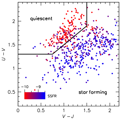
Figure 1.— Distribution of galaxies with $\log M_{\rm stars}>10.6$ $M_{\odot}$ and $2.0<z<2.5$ in the $UVJ$ plane. The galaxies are color-coded by the logarithm of their specific star formation rate, SSFR = SFR/$M_{\rm stars}$. The star formation rates are derived from the UV+IR emission, with the IR emission determined from the Spitzer/MIPS flux. In this paper “star forming galaxies” refers to all objects outside of the $UVJ$ quiescent box.

The distribution of galaxies with $\log M_{\rm stars}>10.6$ and $2.0<z<2.5$ in the $UVJ$ plane is shown in Fig. 1. The quiescent box is indicated with the black lines; galaxies inside this box satisfy the equations

$$V-J < 1.5,$$

$$U-V > 1.3,$$

$$U-V > 0.8(V-J)+0.7.$$ (3)

Galaxies are color-coded by their specific star formation rates, defined as SSFR = SFR/$M_{\rm stars}$, with SFR the star formation rate derived from their UV+IR emission (see Whitaker et al. 2014, and references therein). As can be seen in Fig. 1 the $UVJ$ selection corresponds very well to a selection on specific star formation rate. This was expected from previous studies (e.g., Wuyts et al. 2011); nevertheless, the correspondence is striking as the MIPS 24 $\mu$m measurements (which dominate the star formation rates in this stellar mass range) are entirely independent from the $U-V$ and $V-J$ colors.

We note that a subset of quiescent galaxies has high SSFRs in Fig. 1; these are galaxies whose rest-frame optical/near-IR SEDs show no signs of star formation even though they have high MIPS 24 $\mu$m fluxes. These galaxies are difficult to interpret: they may be quiescent galaxies with an active nucleus, or their star formation is so obscured that the young stars do not contribute significantly to the SED. Fumagalli et al. (2014) show that the optical/near-IR SEDs of these galaxies are very similar to the ones that have no MIPS detection. Approximately 20 % of galaxies in the Barro et al. (2013) sample fall in this category.

Of 582 galaxies with $\log M_{\rm stars}>10.6$ and $2.0<z<2.5$, 185 (32 %) are quiescent and 397 (68 %) are star forming. The total area of the five fields is 896 arcmin², and the number densities of massive quiescent galaxies and massive star forming galaxies are $1.2\times 10^{-4}$ Mpc^-3 and $2.7\times 10^{-4}$ Mpc^-3 respectively. These numbers are consistent with previous measurements from other datasets (e.g., Marchesini et al. 2009; Brammer et al. 2011; Muzzin et al. 2013).

2.3. Selection of Compact Massive Star Forming Galaxies

The size-mass relation for galaxies in the 3D-HST survey with $2.0<z<2.5$ is shown in Fig. 2. Quiescent and star forming galaxies, identified using Eq. 2.2, are indicated with red and blue points respectively. As is well known, star forming galaxies are larger than quiescent galaxies at fixed mass (e.g., Franx et al. 2008; Williams et al. 2010; van der Wel et al. 2014b). Note that the galaxy distribution in Fig. 2 is displaced with respect to that in Fig. 5 of van der Wel et al. (2014b), as we use circularized half-light radii and van der Wel et al. use half-light radii along the major axis.

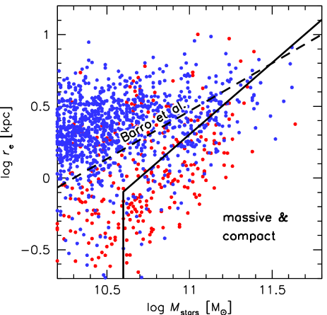
Figure 2.— Size-mass relation for galaxies with $2.0<z<2.5$. Sizes are circularized half-light radii. Red symbols are $UVJ$-selected quiescent galaxies, blue symbols are star forming galaxies. The solid lines shows our selection criteria for compact, massive galaxies: $\log M_{\rm stars}>10.6$ and $\log r_{\rm e}<\log M_{\rm stars}-10.7$. This criterion is more restrictive than that used by Barro et al. (2013, 2014b) (dashed line); we did not use the Barro et al. criterion as 60 % of star forming galaxies with $\log M_{\rm stars}>10.8$ fall below the dashed line, and their median size is significantly larger than that of massive quiescent galaxies.

Compact massive galaxies (CMGs) are in the lower right portion of the size-mass diagram. Barro et al. (2013) use the criterion $\log r_{\rm e}<(\log M_{\rm stars}-10.3)/1.5$ to isolate compact galaxies (dashed line in Fig. 2). However, at masses of $\sim 10^{11}$ $M_{\odot}$ this selection does not produce a sample of compact star forming galaxies that is directly comparable to compact quiescent galaxies. The median size of quiescent galaxies with $\log M_{\rm stars}>10.8$ that satisfy the Barro et al. compactness criterion is $r_{\rm e}=1.3$ kpc. The median size of star forming galaxies with $\log M_{\rm stars}>10.8$ that satisfy this criterion is $2.2$ kpc. For comparison, the median size of the full sample of star forming galaxies with $\log M_{\rm stars}>10.8$ is $2.8$ kpc. That is, at high masses, the Barro et al. criterion selects star forming galaxies whose sizes are closer to those of the full sample of star forming galaxies than to those of compact quiescent galaxies. The reason is that the Barro et al. “compactness” criterion is not very restrictive at high masses, as it selects 60 % of all star forming galaxies that have $\log M_{\rm stars}>10.8$.

As our goal is to select plausible progenitors of massive, compact quiescent galaxies we adopt a slightly more restrictive criterion:

$$\log r_{\rm e}<\log M_{\rm stars}-10.7,$$ (4)

with $M_{\rm stars}$ in units of M_⊙ and $r_{\rm e}$ in units of kpc. This limit is indicated by the solid diagonal line in Fig. 2. Thirty-nine percent of star forming galaxies with $\log M_{\rm stars}>10.8$ satisfy this criterion and their median size is $r_{\rm e}=1.8$ kpc. As we discuss below, the slope of unity of our compactness criterion can be readily interpreted in terms of a physical parameter, namely the velocity dispersion. The slope of $1/1.5=0.67$ used by Barro et al. (2013) was chosen to be consistent with the slope of the size-mass relation of quiescent galaxies as found by Newman et al. (2012). We note that van der Wel et al. (2014b) find a slightly steeper slope than Newman et al. (2012) at $z\sim 2.3$ ($0.76\pm 0.04$ versus $0.69\pm 0.17$).

In addition to their compactness criterion Barro et al. apply a mass limit of $\log M_{\rm stars}>10$. This relatively low limit is also used for their comparison samples of quiescent galaxies and spatially-extended star forming galaxies. However, very few galaxies that have $M_{\rm stars}\sim 10^{10}$ $M_{\odot}$ at $z=2$ will grow into $M_{\rm stars}\sim 10^{11}$ $M_{\odot}$ galaxies by $z=0$ (e.g., van Dokkum et al. 2010; Leja, van Dokkum, & Franx 2013a; Behroozi et al. 2013). We therefore apply a mass limit that is higher by a factor of 4: $\log M_{\rm stars}>10.6$. This selection produces homogeneous samples of massive compact galaxies. Another consideration when choosing this mass limit is that sizes are uncertain when the effective radius is significantly smaller than the pixel size (the drizzled pixel size is $0\farcs 06$, corresponding to 0.5 kpc at $z=2$).

In the remainder of the paper we will use “CMG”, for “Compact Massive Galaxy”, to denote objects with $\log M_{\rm stars}>10.6$ and $\log r_{\rm e}<\log M_{\rm stars}-10.7$. Based on their location in the $UVJ$ diagram we distinguish “qCMG”, for quiescent compact massive galaxy, and “sCMG”, for star forming compact galaxy. There are 112 sCMGs at $2.0<z<2.5$ in the five 3D-HST/CANDELS fields. Five of these have effective radii $r_{\rm e}<0.5$ kpc; when calculating dynamical masses and expected velocity dispersions of these galaxies we use 0.5 kpc instead of their best-fitting radius. It should be noted that many of the star forming progenitors of $2<z<2.5$ qCMGs are expected to be at higher redshift than $z=2.5$; we discuss the evolution of sCMGs and qCMGs in Sections 7 and 8.

2.4. Expected Galaxy-Integrated Velocity Dispersions and Number Densities

We quantify the compactness of galaxies by their expected galaxy-integrated velocity dispersion, as this quantity follows directly from our size-mass selection and can be compared to observations (see Sect. 6.1). For simplicity, we use the following relation:

$$\log\sigma_{\rm pred}=0.5\left(\log M_{\rm stars}-\log r_{\rm e}-5.9\right),$$ (5)

with $\sigma_{\rm pred}$ the predicted velocity dispersion in km s^-1, $M_{\rm stars}$ in units of M_⊙, and $r_{\rm e}$ in units of kpc (Franx et al. 2008; van Dokkum, Kriek, & Franx 2009). This relation has been shown to reasonably predict the observed stellar velocity dispersions of both quiescent galaxies and star forming galaxies, at least in the regime where this has been tested: out to $z\sim 0.7$ for massive star forming galaxies (Taylor et al. 2010a; Bezanson, Franx, & van Dokkum 2015) and out to $z\sim 2$ for massive quiescent galaxies (Bezanson et al. 2013; van de Sande et al. 2013; Belli et al. 2014a).

Our compactness criterion (Eq. 4) corresponds to $\log\sigma_{\rm pred}>2.40$, or $\sigma_{\rm pred}>250$ km s^-1. The distributions of predicted dispersions of sCMGs and qCMGs are shown by the histograms in Fig. 3. The median expected dispersions of the two populations are similar but not identical: $\sigma_{\rm pred}=324$ km s^-1 for quiescent galaxies and $\sigma_{\rm pred}=284$ km s^-1 for star forming galaxies. The reason for this difference is that the size distribution of quiescent galaxies is different from that of star forming galaxies. For star forming galaxies we select the tail of the distribution, with the largest number of galaxies close to the compactness cutoff, whereas for quiescent galaxies we select the bulk of the population (see van der Wel et al. 2014b, for a discussion of the form of the size distributions of quiescent and star forming galaxies). Phrased differently, irrespective of the exact compactness criterion, the smallest galaxies tend to be quiescent. We will return to this in Sect. 8.1, where we define a “quenching line” just inside the compact massive galaxy box.

As shown in Taylor et al. (2010a), the residuals between expected and observed dispersions correlate with the Sersic index. The lines in Fig. 3 show the distributions when the Sersic index of the galaxies is taken into account, using

$$\log\sigma_{\rm pred}=0.5\left(\log G+\log\beta(n)+\log M_{\rm stars}-\log r_{\rm e}\right),$$ (6)

with

$$\beta(n)=8.87-0.831n+0.0241n^{2}$$ (7)

(Cappellari et al. 2006). Here $n$ is the Sersic index and $G=4.31\times 10^{-6}$ when $M_{\rm stars}$ is in units of $M_{\odot}$, $r_{e}$ is in kpc, and $\sigma_{\rm pred}$ is in km s^-1. sCMGs have a slightly smaller median Sersic index ($\langle n\rangle=2.4$) than qCMGs ($\langle n\rangle=2.9$). For quiescent galaxies the line and histogram are nearly the same, but for star forming galaxies the Sersic-dependent dispersions are on average $\approx 10$ % lower than those calculated with Eq. 5.

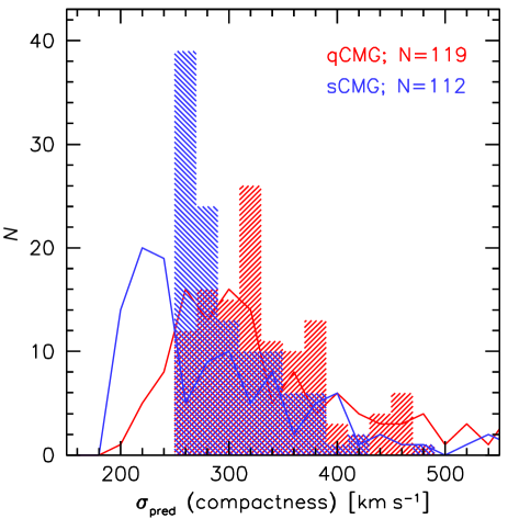
Figure 3.— Distribution of expected galaxy-integrated velocity dispersions at $2.0<z<2.5$, for quiescent compact massive galaxies (qCMGs; red) and for star forming compact massive galaxies (sCMGs; blue). Histograms use a simple relation of the form $\sigma^{2}\propto M_{\rm stars}/r_{\rm e}$. Our compactness criterion corresponds to $\sigma_{\rm pred}>250$ km s^-1. Lines use an expression that takes the Sersic index of the galaxies into account. sCMGs have a median predicted dispersion of $284$ km s^-1.

The number density of qCMGs and sCMGs is the same, $0.8\times 10^{-4}$ Mpc^-3 (for reference, the number density of the full population of quiescent galaxies with $\log M_{\rm stars}>10.6$ is $1.2\times 10^{-4}$ Mpc^-3; see Sect. 2.2). This result is consistent with previous studies that noted the overlap of the compact tail of star forming galaxies and the bulk of the quiescent population (Barro et al. 2013; van der Wel et al. 2014b). We therefore confirm that a population of star forming galaxies can be identified at $2.0<z<2.5$ that has a median mass, median size, and number density similar to the population of massive quiescent galaxies at the same redshifts. If all these compact star forming galaxies quench in the near future, the number density of massive quiescent galaxies will increase by 70 %, and the number density of qCMGs will double.

Table 1Coordinates of Confirmed Star Forming Compact Massive Galaxies

id	RA	DEC	$R_{606}$	$H_{160}$
AEGIS_9163	14h21m03$\fs$68	053°04′37$\farcs$3	25.8	23.2
AEGIS_26952	14h20m40$\fs$81	053°04′51$\farcs$9	25.2	22.2
AEGIS_41114	14h18m32$\fs$92	052°46′06$\farcs$7	25.1	22.7
COSMOS_163	10h00m25$\fs$01	002°10′44$\farcs$1	25.9	23.2
COSMOS_1014	10h00m35$\fs$92	002°11′27$\farcs$8	23.1	21.5
COSMOS_11363	10h00m28$\fs$71	002°17′45$\farcs$4	24.2	21.3
COSMOS_12020	10h00m17$\fs$91	002°18′07$\farcs$2	25.8	22.0
COSMOS_22995	10h00m17$\fs$15	002°24′52$\farcs$3	24.6	22.1
COSMOS_27289	10h00m41$\fs$58	002°27′51$\farcs$5	$\cdots$	22.1
GOODS-N_774	12h36m27$\fs$73	062°07′12$\farcs$8	27.1	23.0
GOODS-N_6215	12h36m06$\fs$86	062°10′21$\farcs$4	25.2	21.5
GOODS-N_13616	12h36m06$\fs$33	062°12′32$\farcs$9	25.9	22.8
GOODS-N_14283	12h37m02$\fs$60	062°12′44$\farcs$0	25.0	22.9
GOODS-N_22548	12h37m00$\fs$46	062°15′08$\farcs$9	25.5	22.5
GOODS-S_5981	03h32m14$\fs$55	$-27$°52′56$\farcs$5	24.9	22.4
GOODS-S_30274	03h32m31$\fs$46	$-27$°46′23$\farcs$2	23.5	21.3
GOODS-S_37745	03h32m43$\fs$88	$-27$°44′05$\farcs$7	24.1	22.0
GOODS-S_45068	03h32m33$\fs$02	$-27$°42′00$\farcs$4	25.0	22.5
GOODS-S_45188	03h32m15$\fs$18	$-27$°41′58$\farcs$7	25.4	22.9
UDS_16442	02h17m20$\fs$80	0$-5$°13′16$\farcs$0	27.4	23.4
UDS_25893	02h18m02$\fs$97	0$-5$°11′21$\farcs$3	$\cdots$	23.1
UDS_26012	02h17m03$\fs$66	0$-5$°11′22$\farcs$2	25.4	22.4
UDS_33334	02h16m55$\fs$01	0$-5$°09′52$\farcs$8	26.2	23.3
UDS_35673	02h17m05$\fs$33	0$-5$°09′25$\farcs$7	25.1	22.4
UDS_42571	02h17m43$\fs$95	0$-5$°07′51$\farcs$3	27.0	22.8

3. Near-IR Spectroscopy

We observed candidate sCMGs with the near-IR spectrographs MOSFIRE (McLean et al. 2012) and NIRSPEC (McLean et al. 1998) on Keck in 2014 and 2015. The resulting spectra provide spectroscopic redshifts (measured from H$\alpha$ and [Nii] at $2.0<z<2.7$), which can be used to verify that a population of sCMGs exists at these redshifts. Furthermore, the spectroscopic observations provide galaxy-integrated kinematics of the ionized gas: if compact star forming galaxies are in the process of forming the stars that are later in compact quiescent galaxies, their gas kinematics should be similar to the stellar kinematics of quiescent galaxies. In addition to redshifts and kinematics the spectra provide star formation rates and strong line ratios; these are important for understanding the physical processes that take place in these galaxies, although their interpretation is often not unique.

3.1. MOSFIRE

The MOSFIRE spectra were obtained in three separate observing runs: January 11, 12 2014; April 18, 23, 25 2014; and Dec 12, 13, 15 2014. The January run suffered from clouds and poor seeing; conditions were generally good during the other two runs. Compact, massive star forming galaxies were not always the main targets, and were not always selected using the criteria of Sect. 2.2. One target from the April run, a galaxy at $z=7.730$, is described in Oesch et al. (2015). The December run gave higher priority to galaxies at $3.0<z<3.6$ than to galaxies at lower redshift. In this paper we will limit the discussion to star forming galaxies at $2<z<2.5$ that satisfy the criteria of Sect. 2.3.

The observations were all taken in the $K$-band, using a standard ABAB dither pattern. The exposure times varied from $\sim 1$ hr to $\sim 4$ hrs, depending on conditions and the requirements imposed by the primary targets in the masks. One of the slits in each mask was devoted to a relatively bright, relatively blue star. This has four important functions: the S/N ratio of the star is used to weight individual exposures in the reduction; the $y-$position of the star is used to correct the data for small vertical drifts of the mask relative to the sky (see Kriek et al. 2015); the extracted spectrum is used to identify regions of strong sky absorption; and the width of the 2D stellar spectrum in the spatial direction provides us with a model of the point spread function (PSF) that is otherwise very difficult to construct (see Sect. 6.2).

The data reduction used the standard MOSFIRE pipeline DRP, with small modifications (see Oesch et al. 2015). Individual sequences were reduced and shifted to a common reference frame before stacking. One-dimensional spectra were obtained from the 2D spectra by summing rows, as dictated by the observed spatial extent of the galaxies. For each mask an empirical noise spectrum was created by removing all rows with signal, and determining the width of the pixel distribution of the remaining rows for each pixel in the wavelength direction. The width was measured by removing the lowest and highest 16 % of values, and is therefore equivalent to the $\pm 1\sigma$ width of a Gaussian. For each individual galaxy in a mask the noise spectrum was multiplied by the square root of the number of rows that was summed to create the 1D spectrum of that object.

3.2. NIRSPEC

The NIRSPEC data were obtained in two runs, January 10, 13, 14 2014 and January 25, 26 2015. Conditions were poor in the 2014 run and the only object in our final sample that came from it is GOODS-N_774, which was published in Nelson et al. (2014). Conditions in 2015 were excellent, with the seeing ranging from $0\farcs 3-0\farcs 6$ during both nights. The selection for the NIRSPEC runs was very similar to that described in Sect. 2.3; within these criteria priority was generally given to galaxies with higher star formation rates (and with good blind offset stars; see below).

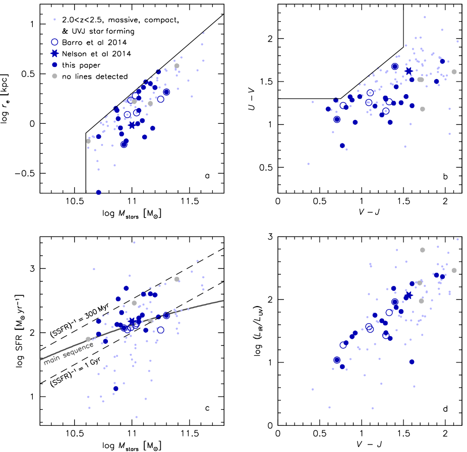
Figure 4.— Comparison of objects with near-IR spectra to the parent population of compact, massive star forming galaxies at $2.0<z<2.5$. Panels show the size-mass relation (a), the $UVJ$ diagram (b), the star formation – mass relation (with the Whitaker et al. (2014) “main sequence” indicated) (c), and the relation between $L_{\rm IR}/L_{\rm UV}$ to the rest-frame $V-J$ color (d). Solid blue symbols are objects in the sample described here. Open symbols are galaxies from Barro et al. (2014b) that fall in our selection box. Grey points are observed galaxies whose spectrum did not show any clear features.

We followed standard observing procedures for NIRSPEC spectroscopy of faint targets (see, e.g., Erb et al. 2003; van Dokkum et al. 2004). Target aquisition was done with blind offsets from nearby stars, as the galaxies are not detected in the SCAM slit-viewing camera. The N6 filter was used for GOODS-N_774; all data in the 2015 run were taken with the N7 filter. A typical observing sequence consisted of four 900 s exposures in an ABBA pattern with $7\arcsec$ offsets between nods. The data were continuously inspected as objects sometimes drift out of the slit.

The data reduction followed standard procedures for near-IR, single slit data (see, e.g., van Dokkum et al. 2004). The data were initially reduced in pairs, using the sky of the A frame for the B frame and vice versa. This method yields relatively clean, photon noise-dominated spectra, at the expense of reducing the S/N in the final frames by $\sqrt{2}$ (see, e.g., Kriek et al. 2015). Wavelength calibration was done using sky lines, which were also used to determine the spectral resolution of the data (see Sect. 3.4.1). The slit is not long enough to obtain an accurate noise spectrum from empty regions; therefore, we calculate the noise spectrum from the sky spectrum and the noise in the darks. An analysis of the residuals from fits to the emission lines shows that this is sufficient for our purposes (see Sect. 3.4.1).

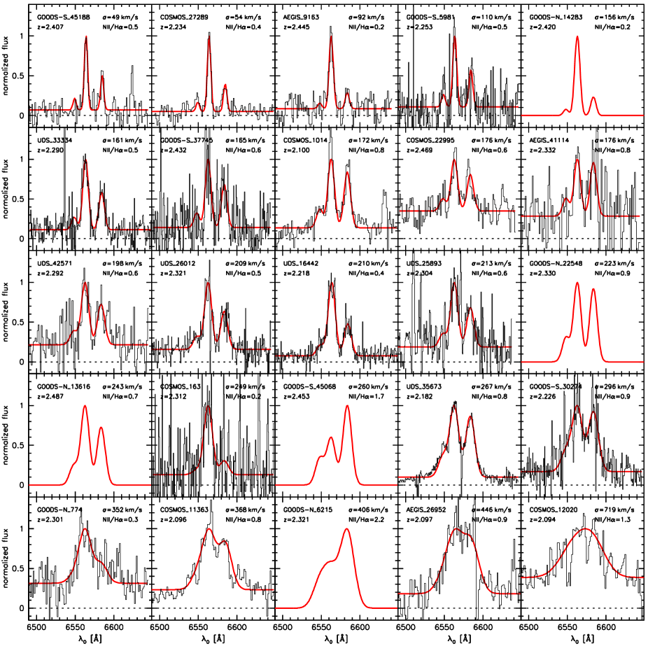
Figure 5.— Spectra of the 20 sCMGs in our sample with $2.0<z<2.5$. Red lines show best-fitting models, as determined with the emcee code (Foreman-Mackey et al. 2013). We also show the best-fitting models of five galaxies from Barro et al. (2014b) that satisfy our selection criteria (red lines without data); these objects are included in our analysis. The galaxies are ordered by their observed line widths, which range from $\sim 50$ km s^-1 to $\sim 700$ km s^-1.

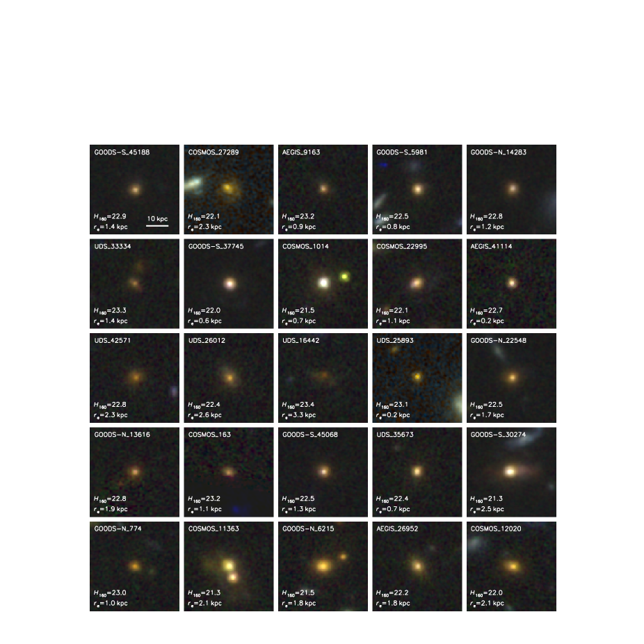
Figure 6.— HST images of the galaxies of Fig. 5, created from the WFC3 $H_{160}$, $J_{125}$ and summed ACS $V_{606}+I_{814}$ images. Each image is $4\farcs 8\times 4\farcs 8$, corresponding to approximately 40 kpc $\times\,40$ kpc. The $H_{160}$ magnitudes and circularized effective radii are listed in the images. Note that the galaxies were selected to be compact in mass, and are not necessarily compact in light. There is generally little evidence for spiral arms, star forming clumps, or other structure. Two galaxies show evidence for past (GOODS-S_30274) and ongoing (COSMOS_11363) mergers. The galaxies are ordered by their H$\alpha$ velocity dispersion, as in Fig. 5. There is no clear relation between HST morphology and H$\alpha$ velocity dispersion in this sample.

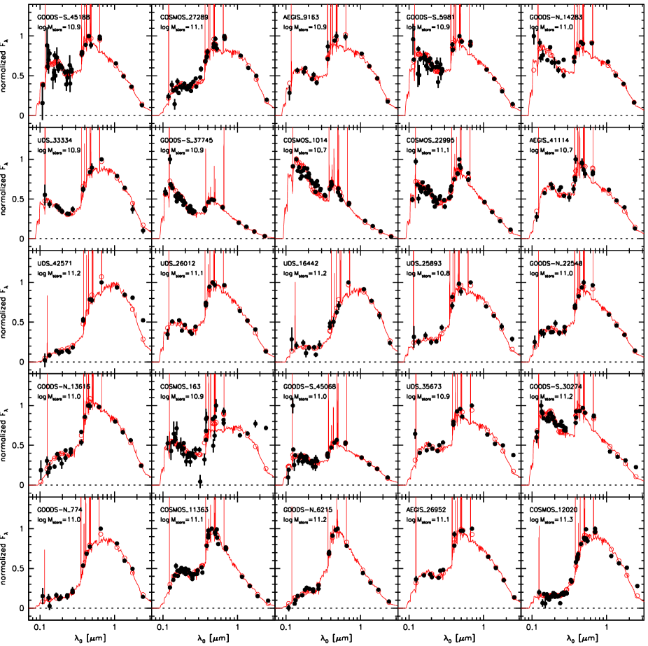
Figure 7.— Restframe UV to near-IR spectral energy distributions of the galaxies of Fig. 5. The red spectra are the best-fitting EAZY (Brammer et al. 2008) models; open red circles show the model fluxes in the observed filters. The SEDs show a large variety, ranging from blue, relatively unobscured emission (COSMOS_1014) to very red SEDs with high inferred dust content (e.g., UDS_42571 and GOODS-N_774). As in Fig. 6, there is no obvious relation between the SEDs of the galaxies and the measured velocity dispersions of their ionized gas.

3.3. Results and Comparison to Parent Sample

We identify the redshifted H$\alpha$ and [Nii] emission lines in 20 out of 24 compact, massive star forming galaxies with expected redshifts in the range $2.0<z<2.5$. This success rate of 86 % is encouraging, but it should be noted that our selection at the telescope was somewhat subjective, particularly in the NIRSPEC runs. As an example, if there were two plausible targets and one showed a hint of an H$\alpha$ contribution to the broad band flux we would generally give it preference. Additionally, there are five non-overlapping galaxies in Barro et al. (2014b) that satisfy our criteria (see Sect. 3.5); the total sample of massive compact star forming galaxies with H$\alpha$ measurements is therefore 25 (Table 1).

The properties of the galaxies in the spectroscopic sample are compared to the parent sample in Fig. 4. The median size and mass are $r_{\rm e}=1.3$ kpc and $M_{\rm stars}=1.0\times 10^{11}$ $M_{\odot}$ respectively, close to the medians of the parent sample. The spread is somewhat smaller; 24 out of 25 galaxies are in the mass range $10.7<\log M_{\rm stars}<11.3$. The galaxies have bluer $U-V$ colors and slightly higher UV+IR star formation rates than the parent sample. This is by selection: galaxies with specific star formation rates ${\rm SSFR}<10^{-9}$ yr^-1 were given lower priority. Despite the lack of galaxies with low star formation rates in the spectroscopic sample, the median SSFR is only 0.1 dex higher than that of the parent sample ($\log{\rm SSFR}=-8.8$ yr^-1 compared to $\log{\rm SSFR}=-8.9$ yr^-1 for the parent sample). Both medians are close to the Whitaker et al. (2014) main sequence for this redshift (dark grey line in Fig. 4c). Panel d of Fig. 4 shows the dust content of the galaxies, as parameterized by both the ratio of the IR and UV luminosities and the rest-frame $V-J$ color. Galaxies in the upper right part of this panel are very dusty, with the re-radiated IR emission exceeding the UV emission by a factor of $>100$. The median $L_{\rm IR}/L_{\rm UV}$ ratio of the parent sample is $\langle L_{\rm IR}/L_{\rm UV}\rangle=64$. The median ratio for the galaxies in the spectroscopic sample is slightly lower, at 42. We only have a few spectroscopic objects in this part of the diagram, and all four spectroscopic failures are located here. We infer that the most likely explanation for the failures is that the H$\alpha$ emission in these galaxies is too obscured for a detection in our current observations.

The Keck spectra of the 20 galaxies that we observed are shown in Fig. 5. The galaxies are ordered by the measured velocity dispersion (see below). We include the five objects from Barro et al. (2014b) that satisfy our selection criteria; as we cannot show the spectra of these objects in Fig. 5, we instead show models that are based on their published best-fitting parameters.

Figures 6 and 7 show the HST images and the rest-frame UV – near-IR spectral energy distributions (SEDs) of the 25 galaxies of Fig. 5. The $H_{160}$ images are shown separately at high dynamic range in Appendix A. The SEDs range from relatively unobscured (COSMOS_1014) to extremely dusty (e.g., GOODS-N_774). Some have excess emission in the IRAC bands (UDS_42571; see, e.g., Mentuch et al. 2009) Two galaxies show clear signs of merging: COSMOS_11363 is an ongoing merger between two compact massive galaxies that are only $0\farcs 6$ apart, and GOODS-S_30274 is probably a merger remnant (see Sect. 7.2). Interestingly, there is no clear relation between the measured velocity dispersion and either the morphology or the SED. Phrased differently, it is not possible to predict the H$\alpha$ line width based on the information shown in Figs. 6 and 7.

3.4. Redshifts, Fluxes, Line Widths, and Line Ratios

3.4.1 Fitting

The spectra were fitted with a model that has the redshift, the continuum level, the [Nii] and H$\alpha$ line fluxes, and the line width as free parameters. The instrumental resolution is explicitly taken into account. The model has the following form:

$$M(\lambda)=L(\lambda)\ast R(\lambda)+C,$$ (8)

with $L(\lambda)$ the model for the line emission, $R(\lambda)$ the instrumental resolution, $C$ the continuum level, and $\ast$ denoting convolution. The instrumental resolution is modeled with a Gaussian:

$$R(\lambda)=\frac{\Delta\lambda}{\sqrt{2\pi}\sigma_{\rm instr}}\exp\left(-0.5\left(\frac{\lambda-\lambda_{\rm cen}}{\sigma_{\rm instr}}\right)^{2}\right),$$ (9)

with $\sigma_{\rm instr}$ measured from sky lines in the vicinity of the redshifted H$\alpha$ line, $\Delta\lambda$ the pixel size in Å, and $\lambda_{\rm cen}$ the center of the fitting range. Expressed as a velocity, the resolution of the MOSFIRE spectra is $\approx 35$ km s^-1, and the resolution of the NIRSPEC data is $\approx 80$ km s^-1. The lines are parameterized as follows:

$$L(\lambda)=f_{{\rm H}\alpha}L_{6563}(\lambda)+f_{[{\rm N}{\textsc{ii}}]}\left(L_{6584}(\lambda)+\frac{1}{3}L_{6548(\lambda)},\right)$$ (10)

with

$$L_{\lambda_{0}}(\lambda)=\frac{\Delta\lambda}{\sqrt{2\pi}\sigma}\exp\left(-0.5\left(\frac{\lambda-(1+z)\lambda_{0}}{\sigma}\right)^{2}\right).$$ (11)

Here $f$ is the line strength, $\sigma$ is the galaxy-integrated line-of-sight velocity dispersion, $\lambda_{0}$ is the rest-frame wavelength of the line (with $\lambda_{0}=6562.8$ and $\lambda_{0}=6548.1$, $6583.6$ for H$\alpha$ and the two [Nii] lines respectively), and $z$ is the redshift.

Some galaxies show evidence for multiple velocity components (e.g., COSMOS_1014). We do not attempt to separately fit broad and narrow velocity components to these galaxies (as was done by, e.g., Förster Schreiber et al. 2014). As discussed later, broad components could indicate the presence of winds but could also indicate rapidly rotating gas at small radii in the galaxies. In the absense of high spatial resolution data, it is difficult to distinguish these possibilities; we therefore simply interpret the H$\alpha$-luminosity-weighted velocity profiles in this paper. It should be noted that the formal uncertainties underestimate the error in the velocity dispersion if the velocity distribution is not Gaussian. This is particularly important for galaxies with a high S/N ratio, such as COSMOS_12020.

The emcee MCMC algorithm (Foreman-Mackey et al. 2013) was used to fit this model to the galaxy spectra. The fit was done over the wavelength region $(1+z)\lambda_{6548}-200<\lambda<(1+z)\lambda_{6584}+200$; the results are not dependent on the choice of fitting region as long as the continuum is reasonably well covered. Priors are top hats with boundaries that comfortably encompass the fitting results. That is, the Bayesian aspects of emcee were essentially turned off. We used 100 walkers and generated 500 chains in each fit. Burn-in was typically fast, but we removed the first 200 chains when calculating errors. For each fit parameter the best fit is defined as the median of the 300 remaining samples. Errors were determined from the 16^th and 84^th percentiles (see Foreman-Mackey et al. 2013, for details). The best fit models are shown by red lines in Fig. 5. Residuals from the fits are shown in Fig. 30. As discussed in Appendix B the residuals are consistent with the expected noise in almost all cases.

3.4.2 Calibration

The redshifts and velocity dispersions follow directly from the MCMC fit, but the line fluxes, equivalent widths, and line ratios need to be calibrated or corrected. The continuum is detected for every galaxy, which makes it possible to calculate equivalent widths directly from the spectra. The equivalent widths, in turn, enable us to calibrate the line fluxes using the known $K$-band magnitudes of the galaxies. The equivalent width of H$\alpha$ in the observed frame is given by

$${\rm EW}_{{\rm H}\alpha}=\Delta\lambda\frac{f_{{\rm H}\alpha}}{C}+{\rm EW}_{{\rm H}\alpha,\,{\rm abs}}(1+z).$$ (12)

The second term is a correction for the underlying stellar continuum absorption, which has a non-negligible effect on the measured equivalent widths and line ratios in our sample. We adopt ${\rm EW}_{{\rm H}\alpha,\,{\rm abs}}=3$ Å (Moustakas & Kennicutt 2006; Alonso-Herrero et al. 2010). The relation between rest-frame equivalent width and the observed equivalent width is ${\rm EW}_{{\rm H}\alpha}^{0}={\rm EW}_{{\rm H}\alpha}/(1+z).$ The mean rest-frame equivalent width in our sample is $\langle{\rm EW}_{{\rm H}\alpha}^{0}\rangle=71$ Å, consistent with the general population of (detected) massive star forming galaxies at these redshifts (Fumagalli et al. 2012). The [Nii]/H$\alpha$ ratio, corrected for absorption, is

$$\frac{[{\rm N}\,{\textsc{ii}}]}{{\rm H}\alpha}=\frac{f_{[{\rm N}{\textsc{ii}}]}}{f_{{\rm H}\alpha}}\times\frac{{\rm EW}_{{\rm H}\alpha}^{0}-{\rm EW}_{{\rm H}\alpha,\,{\rm abs}}}{{\rm EW}_{{\rm H}\alpha}^{0}},$$ (13)

with $f$ taken from the MCMC fit. Note that we use positive values for both absorption equivalent widths and emission equivalent widths in these expressions, as “absorption” here is more accurately described as “emission that is filling in the underlying absorption line”.

The line flux is calculated from the observed equivalent width and the $K$ magnitude using

$$F_{{\rm H}\alpha}=1.02\times 10^{-15}\times\frac{{\rm EW}_{{\rm H}\alpha}}{2730}\times 10^{(K_{s}-22)/-2.5},$$ (14)

with $K_{s}$ the AB magnitude of the object and $F$ in units of ergs s^-1 cm^-2. This expression ignores small differences between the filters used in each field as well as the detailed shape of the continuum within the $K_{s}$ filter. We verified that the transmission at the observed wavelenghts of the lines is within $\sim 5$ % of the central transmission of the filter in all cases. Finally, the line luminosity is calculated using

$$L_{{\rm H}\alpha}=1.20\times 10^{50}\times D^{2}F_{{\rm H}\alpha},$$ (15)

with $D$ the luminosity distance in Mpc and $L$ in ergs s^-1. The results for all galaxies are listed in Table 2. The error bars reflect the (propagated) MCMC errors; no additional calibration uncertainty was included in the error budget.

3.5. Comparison to Barro et al.

There are seven galaxies in the Barro et al. (2014b) sample that satisfy our more restrictive selection criteria. Two of these seven galaxies, COSMOS_12020 and GOODS-S_37745, are also in our sample: COSMOS_12020 was observed with NIRSPEC and GOODS-S_37745 with MOSFIRE. For COSMOS_12020 we find $\sigma=719^{+30}_{-14}$ km s^-1 and [Nii]/H$\alpha$ $=1.39\pm 0.23$, whereas Barro et al. have $\sigma=352\pm 213$ km s^-1 and [Nii]/H$\alpha$ $=0.25\pm 0.25$. The kinematics of this galaxy are very complex, and a Gaussian is a poor fit (see Fig. 5, and Sect. 9.2); this probably explains the differences between the two measurements and the large uncertainty in the Barro et al. values. As noted in Sect. 3.4.1 the formal uncertainty in our measurement of this galaxy is smaller than the true uncertainty, as it does not take deviations from a Gaussian into account. Given that a Gaussian is clearly a poor fit, the velocity dispersion of this galaxy is not well determined. For GOODS-S_37745 we find $\sigma=163^{+27}_{-24}$ km s^-1 and [Nii]/H$\alpha$ $=0.65\pm 0.23$, compared to $\sigma=197\pm 37$ km s^-1 and [Nii]/H$\alpha$ $=0.77\pm 0.30$ in Barro et al. (2014b). These values are in agreement within the (relatively large) $1\sigma$ uncertainties.

For the two galaxies that overlap we use our own measurements. The other five galaxies from Barro et al. are added to our sample (see Tables 1 and 2). We do not have measurements of the line flux or spatial extent of the emission line gas for these objects, but they are included in the analysis whenever only the redshift, velocity dispersion, or line ratio is needed. They are shown in Fig. 5 by their best-fitting models. The total number of sCMGs at $2.0<z<2.5$ that are studied in this paper is 25.

Table 2Properties of Star Forming Compact Massive Galaxies

id	$z$	$M_{\rm stars}$	$r_{\rm e}$	$n$	$q$	SFR	$\log\frac{L_{\rm IR}}{L_{\rm UV}}$	X-ray	instr	$F_{{\rm H}\alpha}$	EW${}^{0}_{{\rm H}\alpha}$	$\sigma$	[Nii]/H$\alpha$
		$10^{11}$ $M_{\odot}$	kpc			$M_{\odot}$ yr-1				$10^{-17}$ ergs s-1 cm-2	Å	km s-1
AEGIS_9163	2.445	0.8	0.9	5.4	0.72	131	1.81		NIRS	$\phantom{0}{}6.6_{-1.3}^{+1.3}$	$\phantom{0}{}74_{-12}^{+12}$	$\phantom{0}{}92_{-18}^{+18}$	$0.21_{-0.07}^{+0.07}$
AEGIS_26952	2.097	1.1	1.8	3.6	0.64	148	1.62	yes	NIRS	$18.4_{-3.2}^{+3.1}$	$\phantom{0}{}95_{-13}^{+13}$	$446_{-54}^{+89}$	$0.90_{-0.14}^{+0.14}$
AEGIS_41114	2.332	0.5	0.2	8.0	0.62	95	1.38		NIRS	$\phantom{0}{}3.2_{-0.7}^{+0.7}$	$\phantom{0}{}30_{-6}^{+6}$	$176_{-37}^{+46}$	$0.85_{-0.24}^{+0.24}$
COSMOS_163	2.312	0.8	1.1	2.5	0.60	336	2.25	yes	MOSF	$\phantom{0}{}7.4_{-2.1}^{+2.3}$	$\phantom{0}{}95_{-26}^{+27}$	$249_{-34}^{+43}$	$0.19_{-0.12}^{+0.12}$
COSMOS_1014	2.100	0.5	0.7	8.0	0.79	150	0.93		NIRS	$18.5_{-2.5}^{+2.5}$	$\phantom{0}{}70_{-6}^{+6}$	$172_{-13}^{+13}$	$0.77_{-0.08}^{+0.08}$
COSMOS_11363	2.096	1.1	2.1	5.2	0.76	169	1.31	yes	NIRS	$22.3_{-2.5}^{+2.4}$	$\phantom{0}{}65_{-3}^{+3}$	$368_{-20}^{+32}$	$0.78_{-0.04}^{+0.04}$
COSMOS_12020	2.094	2.0	2.1	5.7	0.57	185	1.96	yes	NIRS	$\phantom{0}{}8.3_{-1.4}^{+1.4}$	$\phantom{0}{}34_{-5}^{+5}$	$719_{-32}^{+14}$	$1.26_{-0.21}^{+0.21}$
COSMOS_22995	2.469	1.2	1.1	2.8	0.67	188	1.41	yes	NIRS	$\phantom{0}{}5.1_{-0.7}^{+0.7}$	$\phantom{0}{}23_{-2}^{+2}$	$176_{-18}^{+19}$	$0.61_{-0.09}^{+0.09}$
COSMOS_27289	2.234	1.3	2.3	3.3	0.81	398	2.02		NIRS	$25.5_{-3.9}^{+4.0}$	$106_{-12}^{+13}$	$\phantom{0}{}54_{-13}^{+11}$	$0.36_{-0.04}^{+0.04}$
GOODS-N_774	2.301	1.0	1.0	2.9	0.59	150	2.07		NIRS	$\phantom{0}{}5.7_{-0.8}^{+0.8}$	$\phantom{0}{}45_{-4}^{+4}$	$352_{-30}^{+36}$	$0.34_{-0.07}^{+0.07}$
GOODS-N_6215	2.321	1.8	1.8	2.6	0.72	110	1.28	yes	MOSF	$\cdots$	$\cdots$	$406_{-69}^{+69}$	$2.17_{-0.28}^{+0.28}$
GOODS-N_13616	2.487	1.1	1.9	5.6	0.97	130	1.79		MOSF	$\cdots$	$\cdots$	$243_{-30}^{+30}$	$0.73_{-0.18}^{+0.18}$
GOODS-N_14283	2.420	0.9	1.2	2.7	0.86	111	1.43	yes	MOSF	$\cdots$	$\cdots$	$156_{-27}^{+27}$	$0.23_{-0.39}^{+0.39}$
GOODS-N_22548	2.330	1.0	1.7	5.9	0.78	120	1.53	yes	MOSF	$\cdots$	$\cdots$	$223_{-56}^{+56}$	$0.92_{-0.30}^{+0.30}$
GOODS-S_5981	2.253	0.8	0.8	4.4	0.85	206	1.75		MOSF	$\phantom{0}{}8.0_{-1.9}^{+1.9}$	$\phantom{0}{}54_{-11}^{+11}$	$110_{-15}^{+18}$	$0.49_{-0.12}^{+0.12}$
GOODS-S_30274	2.226	1.4	2.5	8.0	0.46	404	1.47	yes	MOSF	$32.6_{-4.6}^{+4.6}$	$\phantom{0}{}81_{-8}^{+8}$	$296_{-17}^{+19}$	$0.90_{-0.08}^{+0.08}$
GOODS-S_37745	2.432	0.9	0.6	3.6	0.94	118	1.04		MOSF	$11.7_{-3.0}^{+3.2}$	$\phantom{0}{}59_{-14}^{+15}$	$165_{-21}^{+27}$	$0.60_{-0.16}^{+0.16}$
GOODS-S_45068	2.453	1.1	1.3	4.9	0.97	139	1.57		MOSF	$\cdots$	$\cdots$	$260_{-18}^{+18}$	$1.70_{-0.78}^{+0.78}$
GOODS-S_45188	2.407	0.7	1.4	4.3	0.90	134	1.66	yes	NIRS	$\phantom{0}{}8.0_{-1.6}^{+1.5}$	$\phantom{0}{}72_{-12}^{+12}$	$\phantom{0}{}49_{-18}^{+17}$	$0.46_{-0.08}^{+0.08}$
UDS_16442	2.218	1.7	3.3	1.6	0.52	176	2.36		MOSF	$15.9_{-2.1}^{+2.2}$	$145_{-12}^{+14}$	$210_{-6}^{+6}$	$0.43_{-0.04}^{+0.04}$
UDS_25893	2.304	0.6	0.2	8.0	0.92	73	1.88	yes	MOSF	$\phantom{0}{}4.9_{-4.1}^{+4.3}$	$\phantom{0}{}54_{-44}^{+46}$	$213_{-23}^{+20}$	$0.58_{-0.28}^{+0.28}$
UDS_26012	2.321	1.3	2.6	3.5	0.73	109	1.47		MOSF	$11.3_{-1.4}^{+1.4}$	$\phantom{0}{}65_{-5}^{+5}$	$209_{-8}^{+7}$	$0.54_{-0.05}^{+0.05}$
UDS_33334	2.290	0.7	1.4	2.4	0.56	13	1.01		MOSF	$\phantom{0}{}6.6_{-3.7}^{+4.8}$	$\phantom{0}{}74_{-41}^{+54}$	$161_{-16}^{+9}$	$0.51_{-0.31}^{+0.31}$
UDS_35673	2.182	0.9	0.7	6.4	0.75	492	2.18		MOSF	$24.7_{-2.6}^{+2.7}$	$136_{-5}^{+5}$	$267_{-3}^{+4}$	$0.84_{-0.02}^{+0.02}$
UDS_42571	2.292	1.6	2.3	1.9	0.82	388	2.39	yes	NIRS	$\phantom{0}{}7.1_{-1.1}^{+1.1}$	$\phantom{0}{}46_{-6}^{+6}$	$198_{-20}^{+22}$	$0.60_{-0.10}^{+0.10}$

4. Interpretation of the Line Ratios and Luminosities

4.1. Line Ratios

Considering that the 25 sCMGs of Fig. 5 were selected in a very restricted region of parameter space, their emission lines show a surprisingly large range of properties. The velocity dispersions range from 50 km s^-1 to $>500$ km s^-1, the [Nii]/H$\alpha$ ratios from 0.2 to $>2$, and the H$\alpha$ line luminosities from $1.3\times 10^{42}$ L_⊙ to $1.2\times 10^{43}$ L_⊙. Two of these parameters, the [Nii]/H$\alpha$ ratio and the velocity dispersion, show a significant correlation: as shown in Fig. 8, galaxies with the highest velocity dispersions tend to have the highest line ratios. The correlation has a formal significance of $>99$ %. The broken line is the best fit relation, which has the form

$$\log\frac{[{\rm N}{\textsc{ii}}]}{{\rm H}\alpha}=(-0.51\pm 0.08)+(1.0\pm 0.2)\log\left(\frac{\sigma_{\rm gas}}{100}\right).$$ (16)

The canonical high-metallicity saturation value for [Nii]/H$\alpha$ in low redshift star forming galaxies is $\sim 0.4$ (e.g., Baldwin, Phillips, & Terlevich 1981; Denicoló, Terlevich, & Terlevich 2002; Pettini & Pagel 2004; Kewley et al. 2013). Although this limit is observed to be higher at $z\gtrsim 2$ (e.g., Brinchmann, Pettini, & Charlot 2008; Steidel et al. 2014; Shapley et al. 2015), values of [Nii]/H$\alpha$$\,>1$ are extreme at any redshift (see, e.g., Leja et al. 2013b; Shapley et al. 2015). A likely explanation for the highest $\sigma$, highest [Nii]/H$\alpha$ galaxies in Fig. 8 is that shocks (Dopita & Sutherland 1995) and/or emission from AGNs (Kewley et al. 2013) are responsible for the line ratios.

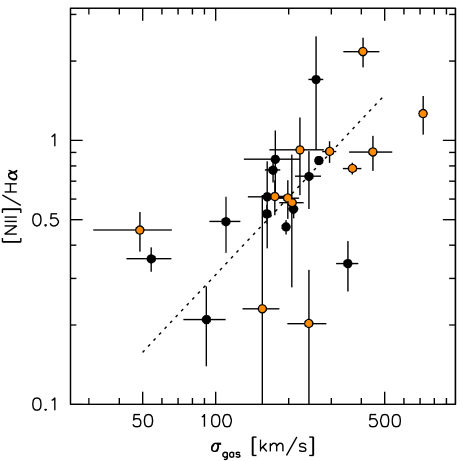
Figure 8.— Relation between [Nii]/H$\alpha$ ratio and H$\alpha$ velocity dispersion for the 25 sCMGs. There is a significant correlation, such that galaxies with higher velocity dispersions have higher [Nii]/H$\alpha$ ratios. Orange symbols are galaxies with X-ray-identified AGN. The four galaxies with the highest observed dispersions are all X-ray AGN, as are five of the six galaxies with the highest [Nii]/H$\alpha$ ratios. The black point with [Nii]/H$\alpha$$=0.3$ and $\sigma=352$ km s^-1  is GOODS-N_774, which was previously published in Nelson et al. (2014).

This is supported by the X-ray luminosities of the objects, obtained from all public catalogs in the CANDELS fields. Twelve of the 25 sCMGs (48 %) have $L_{X}>10^{43}$ ergs s^-1 and are classified as AGN. The X-ray luminosities range from $L_{X}=1.4\times 10^{43}$ ergs s^-1 for GOODS-S_30274 to $L_{X}=6\times 10^{44}$ ergs s^-1 for COSMOS-11363. This high AGN fraction is consistent with previous studies of massive star forming galaxies at these redshifts (e.g., Papovich et al. 2006; Daddi et al. 2007; Kriek et al. 2007; Barro et al. 2013; Förster Schreiber et al. 2014). The four galaxies with the highest velocity dispersions are all classified as X-ray AGN. Their kinematics are complex (see Fig. 5), and their [Nii]/H$\alpha$ ratios range from 0.8 to 2.2. It is likely that the observed emission line properties of these galaxies are affected by the presence of the AGN, either directly through emission from the broad line region or indirectly through AGN-driven winds (see Förster Schreiber et al. 2014; Genzel et al. 2014a).

However, it is not clear whether AGNs or winds dominate the observed, galaxy-integrated kinematics, even for these four objects – and whether the presence of a central point source influenced their selection as apparently compact, apparently massive galaxies. As shown in Fig. 7 the UV – near-IR SEDs of all galaxies are well fit by stars-only models. Most galaxies have strong Balmer breaks (including the most powerful X-ray source in the sample, COSMOS-11363), and as discussed in Kriek et al. (2007) and later studies (e.g., Marsan et al. 2015) this strongly constrains the contribution of continuum emission from an AGN at $\lambda_{\rm rest}\sim 4000$ Å. As we show below and in the following section, the properties of most of the galaxies can be understood in a model where AGN are present but do not dominate the kinematics, line ratios, line luminosities, or morphology.

4.2. Star Formation Rates

The H$\alpha$ luminosities can be converted to star formation rates if it is assumed that the H$\alpha$ emission largely originates in Hii regions. By comparing these star formation rates to those derived from the UV and the bolometric UV+IR luminosities we can assess whether this assumption is reasonable, and also constrain the amount of obscuration in the galaxies. The H$\alpha$ star formation rates were determined using the Kennicutt (1998) relation, converted to a Chabrier (2003) IMF. The UV luminosities come from the best-fitting Brammer et al. (2008) models at $\lambda_{\rm rest}=2500$ Å, and the IR luminosities are converted Spitzer/MIPS 24 $\mu$m fluxes (see Whitaker et al. 2012 and Sect. 2.1).

The relation between the UV/UV+IR star formation rates and the H$\alpha$ star formation rate is shown in Fig. 9. Only the 20 galaxies from our own spectroscopy are considered here, as we do not have self-consistent measurements of $L$(H$\alpha$) for the five objects from Barro et al. (2014b). The H$\alpha$ star formation rates range from 6 $M_{\odot}$/yr – 58 $M_{\odot}$/yr. They correlate with the UV star formation rates (98 % significance) and with the UV+IR star formation rates, which are dominated by the IR (96 % significance). The mean offset between SFR(H$\alpha$) and SFR(UV) is $0.47\pm 0.06$ dex, with an rms scatter of 0.22 dex. The offset between SFR(H$\alpha$) and SFR(UV+IR) is $-1.00\pm 0.09$ dex, with a scatter of 0.27 dex. The implication is that the H$\alpha$ emission misses $\sim 90$ % of the star formation, and the UV misses $\sim 97$ %. The ratios between the three indicators are broadly consistent with expectations from a Calzetti et al. (2000) reddening curve, if there is $\sim 50$ % more dust toward nebular emission line gas than toward the UV continuum.

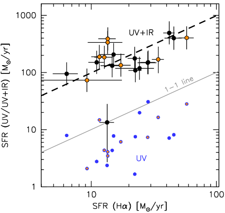
Figure 9.— Relation between the star formation rate derived from H$\alpha$ and the star formation rate derived from the UV (blue points) and UV+IR (black points with errorbars). X-ray AGN are indicated with orange centers. The H$\alpha$ star formation rates fall in between the UV and UV+IR ones, as expected from the effects of dust extinction. The obscuration toward H$\alpha$ is a factor of 10, with a scatter of only a factor of 2. The X-ray sources are indistinguishable from the other galaxies.

The X-ray AGNs are indicated by orange points in Fig. 9. Remarkably, they are indistinguishable from the other objects: they span the same range in H$\alpha$ luminosity, and they follow the same relations with the UV and UV+IR luminosities. The offsets between the AGN and non-AGN are consistent with zero. This suggests, but does not prove, that the H$\alpha$, UV, and IR luminosities of most galaxies are dominated by star formation.

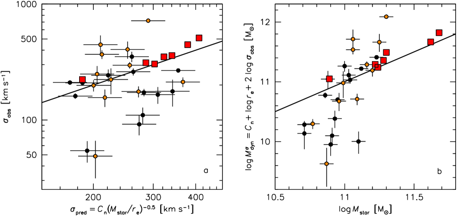
Figure 10.— a) Comparison of observed and predicted velocity dispersions. The predicted dispersions are calculated from the stellar mass, the half-light radius, and the Sersic index. Red squares are quiescent galaxies at $2<z<2.5$ from van Dokkum et al. (2009), van de Sande et al. (2013), and Belli et al. (2014b). Points with errorbars are the 25 sCMGs; orange centers indicate galaxies with X-ray AGN. b) Comparison between dynamical mass and stellar mass. The galaxies show a very large range, and the dynamical masses often appear to be lower than the stellar masses. The gas in sCMGs does not have the same distribution and/or kinematics as the stars in qCMGs.

5. Interpretation of the Velocity Dispersions

5.1. Are the Gas Dynamics Similar to the Stellar Dynamics of Compact Quiescent Galaxies?

The velocity dispersions we measure come from Gaussian fits to the galaxy-integrated, luminosity-weighted H$\alpha$ line profile and are equivalent to the second moment of the velocity distribution of the gas. They should not be confused with the rotation-corrected gas dispersions within spatially-resolved disks, such as discussed by, e.g., Kassin et al. (2012) and Förster Schreiber et al. (2014). The measured dispersions are a complex function of the dynamics and gas distribution in the galaxies:

$$\sigma_{\rm gas}^{2}\sim\alpha^{2}V_{\rm rot}^{2}\sin^{2}(i)+\sigma_{\rm ISM}^{2}+w^{2}(i)\sigma_{\rm wind}^{2},$$ (17)

with $\alpha\sim 0.8$ (Franx 1993; Rix et al. 1997; Weiner et al. 2006; see also Appendix C), $i$ the inclination of the galaxy ($i=0\arcdeg$ is face-on, and $i=90\arcdeg$ is edge-on), $\sigma_{\rm ISM}$ the galaxy-integrated dispersion within the gas clouds, and $w(i)\sigma_{\rm wind}$ an inclination-dependent term that takes non-gravitational motions into account. A further complication is that Eq. 17 is the result of an integral over the area of the galaxy that falls within the slit, weighted by the spatially-varying luminosity of the H$\alpha$ line.

We first assume that the gas in the sCMGs “behaves” in a similar way as the stars in qCMGs. That is, we assume that the stars in qCMGs were formed directly out of the (detected) gas in sCMGs, such that they have the same distribution and kinematics. This has been assumed in previous studies of the kinematics of compact massive star forming galaxies (Nelson et al. 2014; Barro et al. 2014b) and it may be reasonable if many compact, massive quiescent galaxies are direct descendants of the sCMGs. As discussed in Sect. 2.4 the stellar velocity dispersions of quiescent galaxies can be predicted from their stellar masses and effective radii (e.g., Taylor et al. 2010a; Bezanson et al. 2011; Belli et al. 2014b). Figure 10a shows the relation between $\sigma_{\rm gas}$ and the predicted velocity dispersion. The predicted dispersions were calculated using the Sersic-dependent relation Eq. 6.

There is no significant correlation between $\sigma_{\rm gas}$ and $\sigma_{\rm pred}$, for either the full sample or the sample with the X-ray AGN removed. The rms scatter in $\sigma_{\rm gas}/\sigma_{\rm pred}$ is 0.26 dex. Given that we are ignoring the effects of non-gravitational motions, it is striking that many galaxies have lower velocity dispersions than the expectations. The mean offset is $-0.08$ dex for the full sample, and $-0.16$ dex when the AGN are excluded. These results stand in sharp contrast to the stellar velocity dispersions of quiescent galaxies. Red squares are seven galaxies with $2<z<2.5$ and measured $\sigma_{\rm stars}$, $r_{e}$, $n$, and $M_{\rm stars}$ from van Dokkum et al. (2009), van de Sande et al. (2013), and Belli et al. (2014b). They have a mean offset in $\sigma_{\rm stars}/\sigma_{\rm pred}$ of $+0.05$ dex and an rms scatter of only $0.03$ dex.

As dynamical mass is proportional to $\sigma^{2}$ the offsets of the sCMGs are even more dramatic in Fig. 10b, which shows the relation between dynamical mass and stellar mass. Here dynamical mass was calculated using

$$M^{\sigma}_{\rm dyn}=\frac{\beta(n)\sigma_{\rm obs}^{2}r_{e}}{G},$$ (18)

as derived by Cappellari et al. (2006) and following studies of quiescent galaxies at high redshift (e.g., van de Sande et al. 2013). For sCMGs $\sigma_{\rm obs}=\sigma_{\rm gas}$ and for quiescent galaxies $\sigma_{\rm obs}=\sigma_{\rm stars}$. Note that, given our definition of $\sigma_{\rm pred}$ (see Eq. 6), panels a and b of Fig. 10 are two different ways of presenting the same information. The mean mass offset of the sCMGs is $-0.16$ dex for the full sample, and $-0.32$ dex for the sample with the AGN removed. That is, the dynamical masses of the non-AGN galaxies are on average a factor of two lower than the stellar masses. Several of the galaxies have apparent dynamical masses that are a factor of $\gtrsim 10$ lower than their stellar masses. Again, the quiescent galaxies show a tight relation in Fig. 10b, with a mean offset of $+0.1$ dex.

We conclude that the gas dynamics of sCMGs are not similar to the stellar dynamics of quiescent galaxies in the same mass and redshift range. The stellar masses and sizes are not useful indicators of the observed gas velocity dispersions; in fact, the observed [Nii]/H$\alpha$ ratio is a better predictor of the observed H$\alpha$ linewidth of a galaxy than its compactness is. There are many ways to increase the velocity dispersion of a galaxy so it falls above the lines of equality in the two panels of Fig. 10: the broad line region of an AGN, AGN-induced winds, and supernova-driven winds can all lead to broad H$\alpha$ lines (e.g., Westmoquette et al. 2009; Le Tiran et al. 2011; Förster Schreiber et al. 2014; Banerji et al. 2015). This is likely the case for several galaxies in the sample: the four galaxies with the largest dynamical masses are all X-ray AGN with [Nii]/H$\alpha$ ratios in the range $0.8-2.2$. However, it is difficult to decrease the observed dispersion. Setting aside the possibility that the stellar masses of some galaxies could be in error by a factor of $\sim 10$, this is only possible if the detected ionized gas is sCMGs is distributed very differently from the stars in quiescent galaxies. As we show below, there is strong evidence that this is indeed the case.

5.2. Evidence for Rotating Gas Disks

A possible interpretation of the large range of velocity dispersions is that the dynamics are dominated by rotation, and we are seeing disks under a large range of viewing angles. In Fig. 11a we show the distribution of projected axis ratios $q=b/a$ in our sample, as determined from the $H_{160}$ data (see van der Wel et al. 2014b). The axis ratios of the 25 galaxies are inconsistent with a uniform distribution, which would be expected for thin, randomly oriented disks. We find no galaxies with $q<0.4$ and the distribution peaks at $q\sim 0.75$. The distribution is consistent with that observed for qCMGs, shown by the red line in Fig. 11a: according to the Kolgomorov-Smirnov test the probability that both samples were drawn from the same distribution of axis ratios is 27 %. The distributions are also consistent with results for the general population of massive galaxies at $z\sim 2$ (Chang et al. 2013; van der Wel et al. 2014a). We note that we do not detect a significant wavelength dependence of the mean axis ratio of the 25 sCMGs: we find $\langle q\rangle=0.76\pm 0.03$ in $J_{125}$ and $\langle q\rangle=0.74\pm 0.03$ in $H_{160}$.

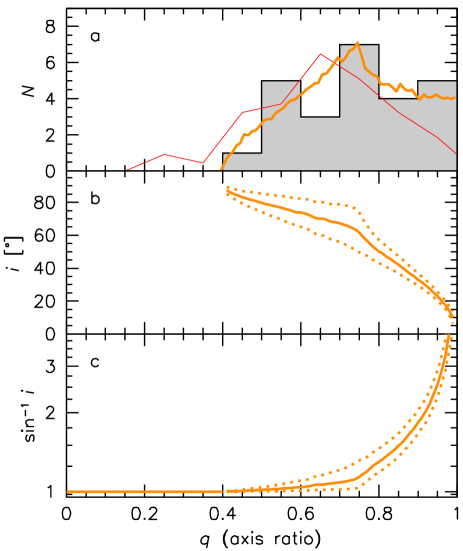
Figure 11.— (a) Distribution of axis ratios among the 25 sCMGs at $2<z<2.5$. The distribution is not uniform, and is inconsistent with thin disks under random viewing angles. The axis ratio distribution of qCMGs in the same redshift range is shown in red. The orange line is a model for randomly oriented oblate objects with intrinsic thickness $q_{0}\equiv C/A=0.4-0.75$. (b) The relation between median inclination and observed axis ratio in this model. Dotted lines indicate the $\pm 1\sigma$ spread. (c) Inclination correction as a function of observed axis ratio.

Even though the stars are not in thin disks, the gas can be. If the gas is in rotationally-supported disks that are aligned with the stellar distribution, the measured velocity dispersions are expected to show an anti-correlation with the observed axis ratios of the galaxies. As shown in Fig. 12a we see precisely this effect: there is an anti-correlation, with a correlation coefficient of $-0.38$ and a significance of 94 %. This is strong evidence that the gas is in disks and that the measured dispersions are dominated by gravitational motions. This anti-correlation is not consistent with M82-style galactic winds: outflows that are perpendicular to the disk lead to the highest observed velocities (and hence integrated velocity dispersions) when the disk is viewed face-on.

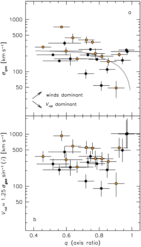
Figure 12.— (a) Observed relation between the H$\alpha$ velocity dispersion and the $H_{160}$ axis ratio. Orange centers indicate X-ray AGN. There is a significant (anti-)correlation between $\sigma_{\rm gas}$ and $q$, as expected if there is a significant contribution from rotation to $\sigma_{\rm gas}$ and the H$\alpha$ disks are aligned with the stellar distribution. The grey line indicates the expected trend for rotating disks (Fig. 11c). (b) Inferred rotation velocity versus axis ratio. The rotation velocities were corrected for inclination using the observed axis ratios (see text). The median rotation velocity is 338 km s^-1 for the full sample and 271 km s^-1 when AGN are excluded.

Going back to Eq. 17, we now assume that $\sigma_{\rm ISM}$ and $\sigma_{\rm wind}$ can be neglected, so that

$$V_{\rm rot}=\frac{\sigma_{\rm gas}}{\alpha\sin^{-1}(i)}.$$ (19)

To derive rotation velocities we need to determine the relation between inclination and axis ratio in our sample. We constructed a model with long, intermediate, and short axes $A$, $B$, and $C$ that reproduces the observed axis ratio distribution for random viewing angles. The orange line in Fig. 11a shows the predicted distribution of $q$ for thick disks – or oblate spheroids – with $A/B=1$ and $q_{0}\equiv C/A$ uniformly distributed between $q_{0}=0.40$ and $q_{0}=0.75$. This model is an excellent fit to the observed distribution of $q$. It should be emphasized that this is a model for the intrinsic shapes of the stellar distribution, not for the gas distribution: the gas is likely in thinner disks, and all we assume is that the gas disks of the galaxies are aligned with their stellar distributions.

For galaxies with intrinsic thickness $q_{0}$ the relation between the inclination and the observed axis ratio is given by

$$\cos^{2}(i)=\frac{q^{2}-q_{0}^{2}}{1-q_{0}^{2}}.$$ (20)

As $q_{0}$ is not a constant in our model the relation between $i$ and $q$ is not single-valued. The solid line in Fig. 11b shows the median relation, and the broken lines indicate the $1\sigma$ scatter. Figure 11c shows the inclination correction $\sin^{-1}(i)$ as a function of $q$.

The inclination-corrected rotation velocities are shown in Fig. 12b. They are derived from the gas velocity dispersions and the observed axis ratios of the galaxies using the average relation in 11c and assuming $\alpha=0.8\pm 0.2$ (see Rix et al. 1997; Weiner et al. 2006). In Appendix C we show that this value is a reasonable approximation for the geometries of both the mass and the ionized gas that we derive in this paper. The large uncertainty reflects the fact that the conversion of dispersion to rotation velocity depends on the spatial distribution of the gas, and the underlying velocity field (see Appendix C). Data of much higher spatial resolution and S/N ratio are needed to measure $\alpha$ directly for these extremely compact galaxies. The uncertainty in $\alpha$ and 50 % of the (logarithmic) inclination correction were added in quadrature to the error budget. The median rotation velocity for the full sample is $\langle V_{\rm rot}\rangle=339$ km s^-1. Excluding the X-ray AGN we find $\langle V_{\rm rot}\rangle=271$ km s^-1.

If it is assumed that $r_{e}$ is not only the half-light radius in the $H_{160}$ band but also the half-light radius of the H$\alpha$ emission, we can define the dynamical mass as

$$M^{V}_{\rm dyn}\equiv 2\frac{V_{\rm rot}^{2}r_{e}}{G}.$$ (21)

This is not a true total mass but simply twice the enclosed mass within the half-light radius. In Fig. 13 this dynamical mass is compared to the stellar mass. Although the inclination corrections have lessened the offsets of the most extreme outliers, it is clear that orientation effects are not sufficient to explain the relatively low velocities that have been measured for a large fraction of the sample. The mean offset for the whole sample is $-0.19$ dex, and the scatter is $0.55$ dex. In the next Section we show that variation in the spatial extent of the ionized gas with respect to that of the stars is a likely source of both the offset and scatter in Fig. 13.

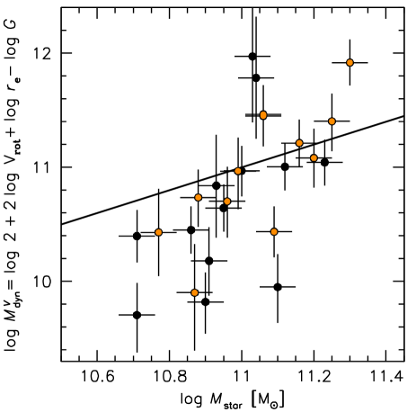
Figure 13.— Relation between dynamical mass and stellar mass, with dynamical masses calculated from the inclination-corrected rotation velocities and the stellar half-light radii. Most galaxies fall below the line of equality.

6. Spatially-Extended Gas Disks

6.1. Inferred Sizes of Gas Disks

In the previous Section we showed that many galaxies have galaxy-integrated velocity dispersions that are much smaller than expected from their stellar masses and sizes. As demonstrated in Sect. 5.2 this is partly caused by the $\sin(i)$ reduction of the velocity of rotating disks. However, even after correcting the observed dispersions to inclination-corrected rotation velocities the dynamical masses are typically lower than the stellar masses, particularly for galaxies that do not host an X-ray AGN.

So far we have assumed that the spatial extent of the gas is similar to that of the stars, that is, $r_{\rm gas}\sim r_{\rm stars}\equiv r_{\rm e}$, where $r_{\rm gas}$ is the half-light radius of the measured H$\alpha$ distribution. There is no a priori reason why this should be the case; e.g., in the models of Zolotov et al. (2015) compact galaxies often have rings of gas and young stars around their dense centers, which originate from ongoing accretion from the halo. Furthermore, as shown earlier $\sim 90$ % of the star formation in sCMGs is obscured, and the extinction is expected to be particularly high toward the central regions (e.g., Gilli et al. 2014; Nelson et al. 2014). The distribution of detected H$\alpha$ emission may therefore be less centrally concentrated than the distribution of star formation.

The radius of the gas disks can be inferred from $V_{\rm rot}$ if we assume that the observed velocity is the circular velocity of the stellar body at the radius of the gas. The gas radius then depends on $V_{\rm rot}$, the stellar mass, and the structural parameters of the galaxy:

$$r_{\rm gas}\sim\frac{G}{V_{\rm rot}^{2}}f(r_{\rm gas})M_{\rm stars},$$ (22)

with $V_{\rm rot}$ the inclination-corrected rotation velocity and $f(r_{\rm gas})$ a function that depends on the mass distribution of the galaxies:

$$f(r_{\rm gas})=\frac{\int_{0}^{r_{\rm gas}}I(r)2\pi r\,dr}{\int_{0}^{\infty}I(r)2\pi r\,dr}.$$ (23)

Here $I(r)$ is the best-fitting Sersic profile to the light distribution. For $r_{\rm gas}=r_{\rm stars}$ ($=r_{\rm e}$), $f(r_{\rm gas})=0.5$ and Eq. 22 is equivalent to Eq. 21 with $M_{\rm dyn}=M_{\rm stars}$. These expressions ignore the fact that the 2D radii are not identical to the 3D radii, assume that the stellar mass distribution can be approximated by the $H_{160}$ luminosity distribution, and assume that the contributions of gas and dark matter to the total mass can be neglected on the scales that are probed by the H$\alpha$ emission.

Solving Eq. 22 numerically, we find that the inferred gas disk sizes range from $\sim 0.2$ kpc to $\gtrsim 10$ kpc. This large range is not surprising, as it is effectively an interpretation of the large variation that is seen in Fig.  13. Figure 14 shows the relation between inferred $r_{\rm gas}$ and the stellar effective radius. The gas radii are typically larger than the stellar radii, particularly for the galaxies that do not have an X-ray AGN (black points). The ratio between the gas radius and the stellar radius is shown explicitly in the bottom panel of Fig. 14. The mean ratio, calculated with the biweight statistic (Beers et al. 1990), is $\log r_{\rm gas}-\log r_{\rm stars}=0.18\pm 0.10$ for the full sample. Excluding galaxies with an AGN, we find $\log r_{\rm gas}-\log r_{\rm stars}=0.37\pm 0.14$. That is, the gas disks are a factor of $\sim 2.3$ more extended than the stellar distribution. This is strictly a lower limit, as it is assumed that only stars contribute to the stellar mass, the galaxies have a relatively “light” Chabrier (2003) IMF, and there are no contributions from non-gravitational motions to the measured velocity dispersions.

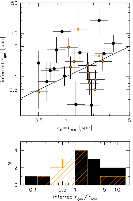
Figure 14.— Relation between inferred radius of the gas distribution and the stellar half-light radius. Orange points indicate galaxies with X-ray AGN. The gas radii were determined from the stellar masses and the inclination-corrected rotation velocities. There is a large scatter, reflecting the large scatter in Fig. 13. The ratio between the gas size and the stellar size is shown in the bottom panel. Non-AGN (black) and AGN (orange) are shown separately. The galaxies with AGN have, on average, compact inferred gas distributions. For the non-AGN (black histogram) the average spatial extent of the gas is $\sim 2.3\times$ larger than that of the stars.

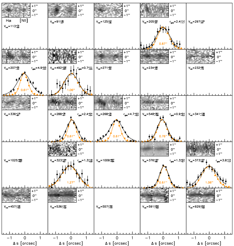
Figure 15.— Two-dimensional MOSFIRE and NIRSPEC spectra centered on the redshifted H$\alpha$ and [Nii] lines. The galaxies are ordered by their observed galaxy-integrated velocity dispersion, as in Figs. 5, 6, and 7. The inclination-corrected rotation velocity $V_{\rm rot}$ (in km s^-1) is indicated in each panel. At least 1/3 of the galaxies show velocity gradients, demonstrating that their ionized gas distributions are spatially resolved in these ground-based, seeing-limited data. For the nine galaxies observed with MOSFIRE the spatial extent of the gas can be measured, using the profile of a star (orange). Black curves are the best fitting exponential profiles convolved with the PSF. The measured half-light radii of the H$\alpha$ emission ($r_{\rm gas}$, in kpc) are indicated.

6.2. Measured Sizes of Gas Disks

We can test directly whether the sCMGs are embedded in large gas disks by examining the observed spatial extent of the emission lines. Even though the galaxies were selected to be extremely compact, the inferred spatial extent of the emission line gas is so large that it should (just) be detectable in ground-based, seeing-limited observations. The 2D spectra are shown in Fig. 15; they cover a rest-frame wavelength range from 6551 Å to 6596 Å and a spatial extent along the slit of $\pm 1\farcs 5$. The five empty panels are the sCMGs from Barro et al. (2014b).

Remarkably, about 1/3 of the galaxies show velocity gradients. They are most prominent in UDS_33334, UDS_26012, and UDS_16442, but also visible in GOODS-S_5981, UDS_42571, and UDS_35673. The seeing ranged from $0\farcs 6$ to $\gtrsim 1\farcs 0$, and the stellar half-light radii of the galaxies are typically $0\farcs 1$. Therefore, the fact that we spatially resolve the H$\alpha$ emission immediately demonstrates that the ionized gas extends to larger radii than the stars in these galaxies. We emphasize here that we do not attempt to measure rotation curves directly from these velocity gradients, as this can only be done reliably when the sizes of galaxies are similar to, or larger than, the spatial resolution of the data (see, e.g., Vogt et al. 1996; Miller et al. 2011; Newman et al. 2013).

For the nine galaxies that were observed with MOSFIRE we can measure the spatial extent of the H$\alpha$ emission. As discussed in Sect. 3.1 a bright star was included in all MOSFIRE masks, and the profile of this star in the spatial direction can be used to approximate the PSF. We extracted spatial profiles of the combined H$\alpha$ and [Nii] emission for the nine galaxies by averaging the data in the wavelength direction. Each column was weighted by the inverse of the noise (which is dominated by sky emission lines); we did not weight by the signal as this would bias the profile towards the central regions. The spatial profiles are shown in Fig. 15 (black points with errorbars). Each panel also shows the profile of the star that was observed in that particular mask (orange points); the FWHM of this profile is also indicated.

The profiles were fit by a model to determine the half-light radii of the ionized gas. The model has the form

$$M(r)=\Sigma(r)\ast P(r),$$ (24)

with $r$ the position along the slit, $\Sigma(r)$ the model for the one-dimensional surface brightness profile of H$\alpha$ along the slit, $P(r)$ a Gaussian fit to the profile of the star, and $\ast$ denoting a convolution. The Gaussian fits to the stellar profiles are shown by orange lines in Fig. 15. Parameterizing $P(r)$ with the sum of two Gaussians does not improve the fit to the stellar profile or change the results. It is not possible to constrain the functional form of the surface brightness profile with our data. Instead, we assume that the H$\alpha$ is in an exponential disk (see Nelson et al. 2013):

$$\Sigma(r)=\Sigma(0)\exp\left(-\frac{1.678|r-r_{\rm cen}|}{r_{\rm gas}}\right).$$ (25)

Here $\Sigma(0)$ is a normalization factor, $r_{\rm cen}$ is the center of the profile, and $r_{\rm gas}$ is the half-light radius of the ionized gas.

We fitted this model to the data using the emcee code, as described for the fits in the wavelength direction in Sect. 3.4.1. Again, the priors are top hats with bounds that do not constrain the fits or the errorbars. Rather than $r_{\rm gas}$ itself we fit $\log r_{\rm gas}$: the error distribution of $r_{\rm gas}$ is highly asymmetric, which means that the peak of the distribution of samples does not coincide with its 50^th percentile. The distribution of the $\log r_{\rm gas}$ samples is symmetric. The resulting measured gas radii, converted to kpc, are listed in the panels of Fig. 15. For seven out of nine galaxies the value of $r_{\rm gas}$ is different from zero with $>2\sigma$ significance.

A geometric correction needs to be applied to the measured values of $r_{\rm gas}$ to account for the fact that the slit is typically not aligned with the major axis of the gas disk. This correction depends on the orientation of the slit and on the inclination of the gas disk:

$$r_{\rm gas}^{\rm c}\approx\left[\cos^{2}\,(i)+\cos^{2}\,({\rm PA}_{\rm slit}-{\rm PA}_{\rm gal})\left(1-\cos^{2}\,(i)\right)\right]^{-0.5}r_{\rm gas}$$ (26)

with $i$ the inclination (as derived in Sect. 5.2), ${\rm PA}_{\rm slit}$ the position angle of the slitmask, and ${\rm PA}_{\rm gal}$ the orientation of the galaxy on the sky (as determined with GALFIT). Note that the corrected $r_{\rm gas}^{\rm c}$ is measured along the major axis (and is not a circularized radius), consistent with our interpretation that the gas is in thin, rotating disks. The median correction is small at 9 %. For GOODS-S_30274 we use the median correction of the other eight galaxies, as its PA mostly reflects the orientation of its tidal tail. We use the corrected radii when comparing the measured radii to predicted radii and when deriving the rotation curve of the galaxies in Sect. 6.4.

For three galaxies, UDS_35673, GOODS-S_30274, and GOODS-N_6215, we obtained an independent measurement of the extent of the emission line gas from their WFC3/G141 grism spectra. These are the only galaxies in the sample of 25 that have grism spectra covering the redshifted [Oiii] $\lambda 4959,5007$ lines and a detection of these lines with $>5\sigma$ significance. As shown in Nelson et al. (2012) emission lines in grism spectra are images of the galaxy in the light of that line, providing direct information on the distribution of ionized gas at $0\farcs 14$ resolution. The interpretation of the [Oiii] lines is complicated by the fact that the two lines are very close together on the detector. We fit the lines simultaneously with GALFIT (Peng et al. 2002), keeping their relative location and flux ratio fixed and using a PSF generated with Tiny Tim (Krist 1995). Two of the three galaxies (UDS_35673 and GOODS-S_30274) are also in the MOSFIRE sample. The best-fit G141 [Oiii] radii of these objects are $1.6\pm 0.3$ kpc and $5.1\pm 1.5$ kpc, in excellent agreement with the MOSFIRE H$\alpha$ values ($1.3^{+0.2}_{-0.1}$ kpc and $3.9^{+1.5}_{-1.4}$ kpc, respectively). The third galaxy, GOODS-N_6215, has a G141 [Oiii] radius of $3.0\pm 1.0$ kpc. In the following, we show all twelve measurements in figures (nine from MOSFIRE, three from HST), with lines connecting the two independent measurements for UDS_35673 and GOODS-S_30274.

6.3. Comparison of Inferred and Measured Sizes

For the ten galaxies with gas size measurements we can directly compare the inferred sizes to the measured ones. The results are shown in Fig. 16. There is a clear correlation, with a significance of $>99$ %. Furthermore, the offset between the two sets of radii is small. Giving equal weight to all twelve measurements we find a difference of only $-0.09\pm 0.07$ dex. This excellent agreement between inferred and measured radii provides support to our modeling of the observed kinematics of sCMGs.

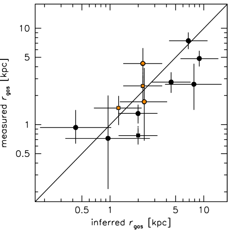
Figure 16.— Relation between inferred and measured half-light radii of the gas distribution in sCMGs. Orange points are galaxies with an X-ray AGN. Circles are Keck/MOSFIRE measurements of H$\alpha$; squares are HST/WFC3 measurements of [Oiii]. Points connected by dotted lines are measurements for the same galaxy. The measured sizes were corrected to account for the difference in orientation between the slit and the galaxy’s major axis. The inferred sizes are based on the observed velocity dispersions, axis ratios, and stellar masses of the galaxies, and the measured sizes are determined directly from the spatial extent of the emission lines. There is a strong correlation, with no significant offset.

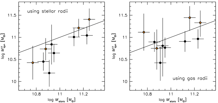
Figure 17.— Dynamical mass versus stellar mass when using the stellar half-light radii (left panel) or the H$\alpha$ half-light radii (right panel) to calculate the dynamical mass. The left panel shows the same information as Fig. 13, but only for the ten galaxies with measured H$\alpha$ radii. The dynamical masses derived from the gas radii are self-consistent, as the rotation velocities were measured at $r_{\rm gas}$, not $r_{\rm stars}$.

This result is presented in a different way in Fig. 17, which shows the relation between dynamical mass and stellar mass. The left panel is identical to Fig. 13, but here we only show the ten galaxies with measured H$\alpha$ effective radii. The dynamical masses in the right panel were calculated using

$$M^{V}_{\rm dyn,\,gas}\equiv\frac{V_{\rm rot}^{2}r_{\rm gas}}{f(r_{\rm gas})G},$$ (27)

with $f(r_{\rm gas})$ accounting for the (small) fraction of the mass that is outside $r_{\rm gas}$ (see Sect. 6.1). The dynamical masses in the right panel are consistent with the stellar masses for all galaxies, although we note that the sample is small. The mean offset is $\log M^{V}_{\rm dyn,\,gas}-\log M_{\rm stars}=-0.07\pm 0.08$, and the rms scatter is 0.25 dex.

Summarizing the results from this and the previous Section, we have inferred that sCMGs have rotating gas disks whose observed spatial extent is larger by a factor of $\sim 2$ than their stellar distribution. This is based on four related results: 1) Many of the galaxies have very low galaxy-integrated velocity dispersions; this shows that the gas does not have the same spatial distribution as the stars and that galactic-scale winds do not dominate the kinematics for the majority of the sample (Fig. 10a). 2) The observed dispersions display a significant anti-correlation with the axis ratios of the galaxies; this is consistent with disks under a range of viewing angles and difficult to reconcile with M82-style galactic winds (Fig. 12a). 3) Nearly all galaxies with spatially-resolved gas distributions show velocity gradients (Fig. 15). 4) Inferring the sizes of the gas disks from the inclination-corrected rotation velocities, we find good agreement between the inferred sizes and the measured sizes (Fig. 16).

6.4. Keplerian Rotation out to 7 kpc

The measured kinematics can be used to constrain the total mass within $\sim 7$ kpc. We can derive a spatially-resolved rotation curve by making use of the fact that the measured spatial extent of the gas varies by a factor of 10 (see Fig. 16), under the assumption that the galaxies have similar inclination-corrected dynamics after scaling them to a common mass. The validity of this approach is demonstrated in Appendix C, where we calculate the relation between the observed galaxy-integrated linewidths and the actual rotation velocity at $r=r_{\rm gas}$. To bring all galaxies to the same normalization, we first define the scaled rotation velocity as

$$V^{\rm s}_{\rm rot}=\frac{V_{\rm rot}}{\sqrt{M_{\rm stars}/\langle M_{\rm stars}\rangle}},$$ (28)

with $\langle M_{\rm stars}\rangle=1.0\times 10^{11}$ $M_{\odot}$ the median stellar mass of the full sample of 25 sCMGs. We note that this scaling does not change the velocities by a large amount as the galaxies in our sample span a small mass range.

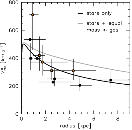
Figure 18.— “Rotation curve” for sCMGs at $2.0<z<2.5$. Points with errorbars are measured inclination-corrected rotation velocities and measured gas effective radii of ten different galaxies. The quantities on the two axes are therefore independent. The velocities were corrected to a common mass of $10^{11}$ $M_{\odot}$  and the radii were multiplied by a factor that accounts for the slit alignment. Galaxies with orange centers have an X-ray AGN. The rotation curve declines, with $>99$ % significance. The black curve is not a fit, but the expected rotation curve if all the mass is in the compact stellar component of the galaxies. This model is a good description of the data. The grey curve assumes that 50 % of the total mass is in the form of gas, with a spatial extent that is a factor of 2.5 larger than that of the stars. This model is inconsistent with the data.

In Fig. 18 the scaled velocities are plotted as a function of the measured gas half-light radius $r_{\rm gas}$ (corrected for slit orientation) for the 10 galaxies that have this measurement. The rotation curve declines: in galaxies where H$\alpha$ is measured at a larger distance from the center, the inclination-corrected rotation velocity is lower. The decline has a formal significance $>99$ %. Falling rotation curves have been seen previously in some individual (large, non-compact) $z\sim 2$ galaxies (e.g., the galaxies D3a6397 and zC400690 in Genzel et al. 2014b). The solid line is the predicted rotation curve for an $M=10^{11}$ $M_{\odot}$ galaxy with the median effective radius ($r_{e}=1.3$ kpc) and median Sersic index ($n=4$) of the sCMGs, calculated with Eq. 22. This model is a good description of the data: $\chi^{2}=6.5$ with 12 degrees of freedom. The grey line is a model with two mass components: in addition to the stellar component this model has a gas component with the same mass as the stars (i.e., the gas fraction in this model is $f_{\rm gas}\equiv M_{\rm gas}/(M_{\rm stars}+M_{\rm gas})=0.5$). For consistency with the previous Sections, the spatial distribution of the gas is assumed to be exponential with $r_{\rm gas}=2.5\times r_{e}$. The grey line overpredicts the observed velocities: with $\chi^{2}=30.0$ this model can be ruled out with $99$ % confidence.

We can derive an upper limit to the gas mass within 7 kpc by assuming that the uncertainty in the stellar mass is small and allowing the mass in the gas component to vary. The 95 % confidence upper limit to the gas mass is $M_{\rm gas}<0.6\times 10^{11}$ $M_{\odot}$, corresponding to a limit on the gas fraction of $f_{\rm gas}<0.4$. It appears that the gas is mostly a tracer of, rather than a contributor to, the kinematics. Finally, we derive the best fitting mass within $r=7$ kpc by assuming that $f_{\rm gas}=0$ and allowing $M_{\rm stars}$ to vary: $M_{\rm fit}=0.8^{+0.6}_{-0.4}\times 10^{11}$ $M_{\odot}$, where the errorbars are 95 % confidence limits. Although this estimate assumes that mass follows light, we verified that the results are very similar for more extended mass distributions. We conclude that the dynamical mass within $r\sim 7$ kpc is fully consistent with the stellar mass that is implied by the stellar population fit; and that there is little room for additional stars, gas, or dark matter inside this radius.

7. Are Star Forming Compact Galaxies the Main Progenitors of Quiescent Compact Galaxies?

In the previous Sections we have shown that a population of star forming galaxies exists at $z\gtrsim 2$ whose dynamical mass within $\sim 7$ kpc is dominated by a massive, compact, stellar component. We now ask whether these galaxies can be progenitors of the population of massive, compact, quiescent galaxies, by considering their number densities, morphologies, and star formation rates. This question has been discussed before, by, e.g., Williams et al. (2014, 2015), Bruce et al. (2014), Nelson et al. (2014), Dekel & Burkert (2014), Zolotov et al. (2015). Arguably the most extensive observational study is a series of papers by Barro et al. (Barro et al. 2013, 2014a, 2014b), using data over two (Barro et al. 2013, 2014b) or one (Barro et al. 2014a) of the five fields that we study here. Using our larger data set and more restrictive selection we find broadly similar results.

7.1. Number Density Evolution

A star forming compact massive galaxy will resemble a quiescent compact massive galaxy if star formation stops (quenching). However, the opposite is also true: a quiescent compact galaxy that starts forming stars due to the accretion of new gas (see, e.g., Zolotov et al. 2015; Graham, Dullo, & Savorgnan 2015) could resemble a star forming compact galaxy (rejuvenation). We can determine whether quenching or rejuvenation dominates by measuring the number density of sCMGs and qCMGs as a function of redshift. The selection criteria of Sect. 2.3 were applied in small redshift bins, and the number density was determined by dividing the number of galaxies in the bin by its volume. The result is shown in Fig. 19 (filled points and solid curves).

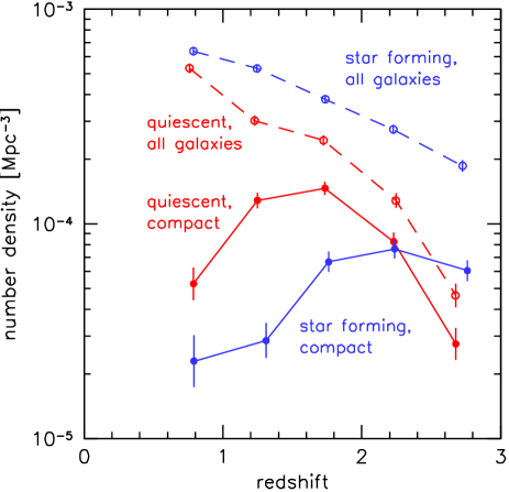
Figure 19.— Evolution of the number density of sCMGs (blue solid line) and of qCMGs (red solid line). The number density of all star forming and quiescent galaxies with $\log(M_{\rm stars})>10.6$ is also shown (dashed lines). The data suggest that compact star forming galaxies continuously enter the selection region from $z\gtrsim 2.8$ to $z\sim 1.8$ and quench, leading to a strong increase in the number of compact quiescent galaxies. When the number of sCMGs begins to decrease at $z<1.8$, the number of qCMGs first plateaus and then drops, as quiescent galaxies grow in size due to mergers at $0.5<z<1.5$.

At $2.0<z<2.5$ the number densities of the two populations are very similar, as already noted in Sect. 2.4. However, at higher and lower redshifts the number densities are different: the sCMGs have a roughly constant number density from $z\sim 2.8$ to $z\sim 1.8$, whereas the number density of qCMGs increases by an order of magnitude over that same redshift range. A straightforward interpretation is that star forming galaxies continuously enter the “compact massive” selection box (because of a decrease in their size and/or an increase in their mass), and quench shortly after. This continuous quenching then leads to a rapid build-up of the number of quiescent galaxies in the compact/massive selection region. We conclude that quenching likely dominates over rejuvenation: if rejuvenation dominated, we would have expected to see quiescent galaxies disappear as their star formation (re-)started, unless there are other channels to create quiescent compact galaxies. We note that the evolution of the number densities of the two populations is qualitatively similar to the simulations of Zolotov et al. (2015).

It is difficult to determine how long it takes before a compact star forming galaxy turns into a quiescent galaxy, as this depends on the rate with which new galaxies enter the sample. The number density of sCMGs is constant from $z\sim 2.8$ to $z\sim 1.8$, which means that new sCMGs enter the sample at approximately the same rate as existing ones quench. We can obtain a very rough estimate of the “compact life time” of star forming galaxies $\tau_{\rm c}$ by adding the number densities of the sCMGs in the three redshift bins that cover this period: if the average quenching time is much shorter than the time interval between redshift bins, all galaxies in each bin are new arrivals and should be added to the sample of progenitors of quiescent galaxies. The combined number density in these bins (which are of nearly equal volume) is $2.0\times 10^{-4}$ Mpc^-3, higher than the increase in the number density of the qCMGs over this period ($1.3\times 10^{-4}$ Mpc^-3). This implies that only about half of the star forming galaxies disappear from one redshift bin to the next, and that the average quenching timescale is roughly equal to the time interval between the redshift bins: $\tau_{\rm c}\sim 0.5$ Gyr. This is the average lifetime of star forming galaxies in the “compact massive” selection box, assuming that they all turn into quiescent galaxies. It is slightly lower than the value of $\sim 0.8$ Gyr derived by Barro et al. (2013), but judging from their Fig. 5 the two studies are broadly consistent.

Although somewhat outside of the scope of this paper, we briefly discuss the number density evolution at lower redshift. The number density of sCMGs drops precipitously after $z\sim 1.8$. This drop leads to a plateau in the number density of qCMGs: as the number of star forming progenitors decreases, no new quiescent galaxies are added to the sample. At the lowest redshifts the number density of compact quiescent galaxies decreases (as was also found by Taylor et al. 2010b, van der Wel et al. 2014b, and van Dokkum et al. 2014, among others), while the number density of all massive quiescent galaxies rises steeply (dashed red curve). The likely explanation is that the compact galaxies accrete extended envelopes through merging from $z\sim 1.5$ to the present day (e.g., Bezanson et al. 2009; Naab et al. 2009; van Dokkum et al. 2010, 2014; Newman et al. 2012; Hilz et al. 2013).

Finally, we note that Fig. 19 is not new: the peak in the number density of compact, massive quiescent galaxies was also shown in Cassata et al. (2011, 2013), Barro et al. 2013, and van der Wel et al. (2014b). Barro et al. (2013) derive a similar lifetime for star forming galaxies in the compact selection region. Although uncertainties remain (particularly at low redshift; see, e.g., Carollo et al. 2013), it is encouraging that these largely independent samples give similar results.

7.2. Morphologies and Radial Surface Brightness Profile

The large spatial extent of the ionized gas raises the question whether the stellar half-light radii and masses of the compact star forming galaxies have been underestimated: although it is difficult to bias GALFIT measurements in this direction (see, e.g., Davari et al. 2014), it is possible that the galaxies have extended low surface brightness envelopes (see, e.g., Hopkins et al. 2009a). If such envelopes exists this would call into question whether sCMGs can be direct progenitors of compact quiescent galaxies with the same apparent mass and half-light radius.

Images of the galaxies are shown in Fig. 6 and in Fig. A1 (see Sect. 3.3). Visually, most of the objects have a compact luminosity distribution and no spiral arms, clumps, star forming complexes, or other features outside of the dense center. Several of the reddest galaxies do not appear very compact: for example, UDS_42571 and, in particular, UDS_16442 are faint and fuzzy rather than bright and compact. The reason for their relatively low surface brightness is that dust obscuration has dramatically lowered their luminosity: as galaxies can have high $M/L$ ratios, compact in mass does not necessarily imply compact in light.

Two objects show unambiguous evidence for ongoing or past mergers: GOODS-S_30274 has an asymmetric feature resembling a tidal tail, and COSMOS_11363 is one component of a spectacular merger between two compact galaxies with a projected separation of $0\farcs 6$ (5 kpc). The companion of COSMOS_11363 is COSMOS_11337 in the Skelton et al. (2014) catalog. Our Keck/NIRSPEC and HST/WFC3 spectroscopy confirms that they are at the same redshift. With $r_{e}=1.0$ kpc and $M_{\rm stars}=1.7\times 10^{11}$ $M_{\odot}$ COSMOS_11337 is actually significantly more compact than COSMOS_11363. Its rest-frame $UVJ$ colors (just) give it a quiescent classification. This merging pair seems to suggest that CMGs can form in mergers (Hopkins et al. 2009b), but that is not the right interpretation: as both galaxies already fall in the “compact massive” selection region, this particular type of merger actually decreases their number. Even if the result of the merger falls in the selection region, there will be one less CMG. Interestingly, several other galaxies show evidence for distorted outer isophotes in Fig. A1. This could indicate interactions are common for these galaxies, but the evidence is not conclusive at the depth of the CANDELS imaging.

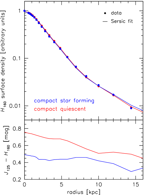
Figure 20.— Radial surface brightness profile, measured from a stack of all 25 sCMGs in our spectroscopic sample (blue points). The profile is very well fit by a single Sersic profile, convolved with the PSF (blue line). There is no excess emission at large radii. For comparison, the red points and red line are for qCMGs that were selected to have the same median size and mass as the sCMGs. Their profile is virtually identical to the star forming galaxies. The bottom panel shows color profiles for both samples. The galaxies have modest color gradients, with the outskirts slightly bluer than the centers.

To quantify the stellar emission on scales $\gg 1$ kpc we stacked the $H_{160}$ images of the 25 sCMGs and measured their averaged radial surface brightness profile to faint levels. Each galaxy was normalized by its total $H_{160}$ flux prior to stacking, so that the stack is not dominated by a few bright objects. Neighboring objects, identified from the SExtractor segmentation map (see Bertin & Arnouts 1996; Skelton et al. 2014), were masked. The resulting surface brightness profile is shown in the top panel of Fig. 20 (blue points). We fit the stack with a PSF-convolved Sersic profile to determine whether there is evidence for an additional component at large radii. This fit, done with GALFIT (Peng et al. 2002), is shown by the blue line. It is an excellent description of the data out to 15 kpc ($>10r_{e}$): there is no excess light beyond a single Sersic profile. Furthermore, the best-fitting effective radius ($r_{e}=1.3$ kpc) and Sersic index ($n=3.6$) are similar to the median values of the 25 galaxies that went into the stack: $\langle r_{e}\rangle=1.4$ kpc and $\langle n\rangle=4.3$.

The stacked sCMG profile is compared to a stacked qCMG profile, shown in red in Fig. 20. The qCMGs in this Figure are a subset of the full population: they were selected in narrow bins of mass and effective radius, centered on the median values of the 25 sCMGs. This ensures that any differences between the stacks are not caused by a difference in the mean size or mass of the samples. The quiescent profile is virtually indistinguishable from that of the star forming galaxies. Finally, $J_{125}-H_{160}$ color profiles of both stacks are shown in the bottom panel of Fig. 20. Both stacks are bluer at larger radii and the gradients are small, qualitatively consistent with previous work (Szomoru, Franx, & van Dokkum 2012). The negative color gradients imply that the galaxies are even more compact in mass than in light, and that any stellar emission at $r\gg r_{e}$ is not missed because it is enshrouded in dust.

We conclude that the morphologies of the sCMGs are consistent with being direct progenitors of qCMGs. When selected to have the same mass and effective radius, their surface brightness profiles are indistinguishable out to at least 15 kpc. We find a relatively high Sersic index for both populations. Such high values (and the relatively round 3D morphologies; see Sect. 5.2) are consistent with violent relaxation following a merger, but also with composite structures, such as envelopes of material around extremely compact exponential disks.

7.3. Star Formation Rates and Gas Content

Accepting that the sCMGs are direct progenitors of qCMGs, an important question is whether they are forming a large fraction of the stars that are present in their quiescent descendants. If the life times of the sCMGs are short, or the star formation rates are low, they may account for only a small fraction of the total stellar mass in compact massive galaxies at $z\sim 2$. We address this question in Fig. 21, which shows the relation between the specific star formation rate and compactness within the sample of compact, massive galaxies at $2<z<2.5$.

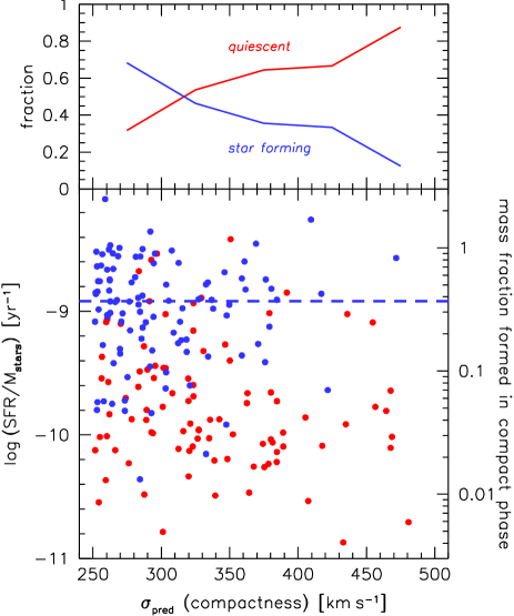
Figure 21.— Relation between specific star formation rate and compactness ($\propto M_{\rm stars}/r_{\rm e}$), for galaxies in the “massive, compact” selection box at $2<z<2.5$. Red points are $UVJ$ quiescent galaxies; blue points are $UVJ$ star forming galaxies. Within the sample of massive compact galaxies, the specific star formation rate, and the fraction of $UVJ$ star forming galaxies, declines with the degree of compactness. The right axis is the fraction of mass that will be added to the galaxies in 0.5 Gyr, which is the estimated average lifetime of star forming galaxies in the massive, compact region. About $1/3$ of the mass of compact quiescent galaxies was formed in the compact phase.

The right axis of this figures shows the fraction of the total stellar mass that is formed in the compact phase:

$$\frac{M_{\rm c}}{M_{\rm stars}}\sim{\rm SSFR}\times w\times\tau_{c},$$ (29)

with SSFR the specific star formation rate, $w$ a correction for mass loss due to stellar winds, and $\tau_{c}$ the average life time of star forming galaxies in the compact, massive selection region. The median specific star formation rate of the sCMGs is SSFR $=1.2\times 10^{-9}$ yr^-1, and for $w\sim 0.6$ (Chabrier 2003) and $\tau_{c}\sim 0.5$ Gyr (Sect. 7.1) we find $M_{\rm c}\sim 0.4M_{\rm stars}$. As they are, on average, observed halfway through their lifetime in the compact selection region, their final mass before quenching will be $M_{\rm stars,final}=M_{\rm stars}+0.5M_{\rm c}\sim 1.2M_{\rm stars}$, and the fraction of $M_{\rm stars,final}$ that is formed in the compact phase is then $\sim 1/3$. We conclude that sCMGs are responsible for forming a significant fraction of the stars that are present in compact quiescent galaxies.

An implication of this result is that the spatial distribution of the H$\alpha$ emission in sCMGs is probably more extended than the spatial distribution of star formation in these galaxies. This is qualitatively similar to results for galaxies at $z\sim 1$ (Nelson et al. 2012, 2015), and may indicate that star formation has ceased in the inner regions of the galaxies (e.g., Genzel et al. 2014b; Tacchella et al. 2015). However, as discussed in Sect. 4.2 most of the star formation in sCMGs is obscured, and the observed H$\alpha$ emission accounts for only $\sim 10$ % of the total star formation. As the column density is a very strong function of radius in these compact galaxies (see, e.g., Gilli et al. 2014; Nelson et al. 2014), the obscuration-corrected distribution of star formation is almost certainly much more compact than the observed distribution of H$\alpha$ emission – at least for the galaxies with low observed velocity dispersions.

A somewhat puzzling aspect of the sCMGs is that they have very high specific star formation rates even though their observed kinematics leave little room for a large gas reservoir (see Sect. 6.4). Many studies have found that the molecular gas and dust content of galaxies increases with redshift, and reaches $>50$ % of the total baryonic mass for $z\sim 2$ galaxies with the highest star formation rates (e.g., Tacconi et al. 2010; Daddi et al. 2010; Genzel et al. 2015; Scoville et al. 2015). Using the scaling relations derived in Genzel et al. (2015), the expected gas fraction for the galaxies in our sample is $\sim 60$ %. One possible explanation for their relatively low gas fraction is that the galaxies have nearly exhausted their reservoir and are about to quench. If the galaxies typically build $\sim 40$ % of their mass inside the compact, massive selection region, the average sCMG should have $\sim 30$ % of their mass in gas (for $w\sim 0.6$); this is just consistent with the 95 % confidence upper limit on the gas fraction of 40 % that we derived in Sect. 6.4. Another explanation is that newly accreted gas is continuously and efficiently funneled into the central regions, and the star formation rates are “accretion throttled” (Dekel et al. 2009); in that case the gas depletion time can be shorter than the actual duration of star formation (see, e.g., Genzel et al. 2010). Direct observations of the dust and molecular gas in sCMGs, at $\sim 1$ kpc resolution, are needed to address these questions.

Finally, we note that star forming galaxies tend to be less compact than quiescent galaxies even within the population of compact massive galaxies at $2<z<2.5$ (see Fig. 21). As discussed earlier in the context of the sample selection (Sect. 2.4), star forming galaxies are always less compact than quiescent galaxies, irrespective of the precise criteria for their selection. In the next Section we interpret the distribution of galaxies in the size-mass plane in the context of a simple model, in which star forming galaxies become gradually more compact and the probability of quenching rises smoothly as their compactness increases.

8. Formation of Star Forming Compact Galaxies

8.1. A Simple Model for Building Massive Galaxies

In this Section we turn to the formation of compact, massive star forming galaxies. Several distinct mechanisms have been discussed in the literature, including mergers of gas-rich galaxies (Tacconi et al. 2008; Hopkins et al. 2009b; Hammer et al. 2009; Wellons et al. 2015), in-situ, inside-out growth of even more compact progenitors (Oser et al. 2010; Johansson, Naab, & Ostriker 2012; Williams et al. 2014; Nelson et al. 2014; Wellons et al. 2015), “compaction” of the gas in star forming galaxies due to disk instabilities (Dekel & Burkert 2014), and hybrid models that include several of these effects (Zolotov et al. 2015).

Although individual massive galaxies likely have complex formation histories, including periods of compaction, mergers, and star bursts, the population of massive galaxies should follow a particular track in the size-mass plane that is determined by the dominant mode of growth when the evolution of many galaxies is averaged. Tracks derived from observations and simulations are shown in Fig. 22. The blue and red tracks show the evolution of galaxies matched by their cumulative number density, for (relatively) low mass galaxies (van Dokkum et al. 2013, blue) and high mass galaxies (Patel et al. 2013, red). The solid parts of the curves are for $1.5<z<3$ and the dotted parts for $0<z<1.5$. Low mass galaxies evolve along a single track with a slope of $\sim 0.3$. High mass galaxies evolve along a similar track from $z\sim 3$ to $z\sim 1.5$ but then turn “upward”, around the time when star formation ceases and the growth becomes dominated by dry mergers (see Sect. 9.1).

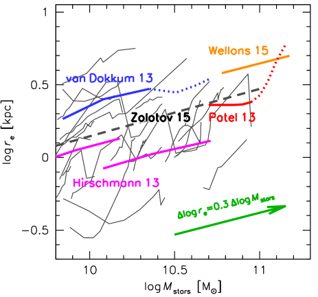
Figure 22.— Tracks of galaxies in the size-mass plane in different studies. The solid blue and red curves show the evolution from $z\sim 3$ to $z=1.5$ of number density-matched samples of low mass (van Dokkum et al. 2013) and high mass (Patel et al. 2013) galaxies. Broken curves show the evolution at $z<1.5$. Magenta tracks are the wind models of Hirschmann et al. (2013), for two different mass ranges and $1.5<z<2.5$. The orange curve is the evolution of the full sample of massive Illustris galaxies from $z=3$ to $z=1.5$ in Wellons et al. (2015). Thin black curves are individual simulated galaxies in Zolotov et al. (2015), from $z=3$ to $z=1.5$. The mean Zolotov evolution is indicated by the thick black dashes. The green arrow is a good match to the mean growth of galaxies in all these studies: $\Delta\log r_{\rm e}\sim 0.3\Delta\log M_{\rm stars}$.

Magenta, orange, and black curves are from simulations. The magenta tracks are the wind models shown in Fig. 10 of Hirschmann et al. (2013), for two different mass ranges. These models are the same as those in Genel et al. (2012), and are updated versions of the momentum-driven wind models of Oppenheimer & Davé (2006) in cosmological simulations. They include both winds and metal enrichment; as shown in Hirschmann et al. (2013) models without winds predict somewhat steeper relations between size growth and mass growth. The orange curve is the track of galaxies in the Illustris project (Vogelsberger et al. 2014), as shown in Fig. 5 of Wellons et al. (2015). This is the average track of all galaxies with a stellar mass in the range $1-3\times 10^{11}$ $M_{\odot}$ at $z=2$. The thin black curves show the evolution from $z=3$ to $z=1.5$ of individual galaxies in the simulations of Zolotov et al. (2015). We include all 34 simulations, irrespective of whether they have a “compaction” phase. The thick dashed curve was created by averaging the evolution in these simulations. The number density-matched observational samples and the simulations all suggest that the ensemble-averaged evolution of star forming galaxies in the size-mass plane is well approximated by

$$\Delta\log r_{\rm e}=0.3\Delta\log M_{\rm stars},$$ (30)

that is, galaxies increase their size by a factor of 2 for every factor of 10 evolution in their mass. This simple inside-out growth model is qualitatively consistent with a host of other data and theory, including the expected growth of disks in $\Lambda$CDM (e.g., Mo, Mao, & White 1998) and the distributions of star formation and existing stars in galaxies (e.g., Nelson et al. 2012). Interestingly, this track corresponds to an approximately constant 3D density within the effective radius (as $\rho(r_{\rm e})\propto M/r_{\rm e}^{3}$, it follows that $r_{\rm e}\propto M^{1/3}$ if the density is constant).

Although the 3D density within the effective radius stays constant, a direct consequence of Eq. 30 is that the stellar density within a physical radius, the stellar surface density, and the stellar velocity dispersion all gradually increase as galaxies form stars. We assume that galaxies have an increasing likelihood of quenching as their velocity dispersion reaches a particular threshold. This is motivated by numerous studies showing that the specific star formation rates of galaxies correlate much better with compactness than with mass (e.g., Kauffmann et al. 2003; Franx et al. 2008). We parameterize this process by a dispersion-dependent quenching probability $P_{\rm q}$:

$$P_{q} = 0\,\,\,\,\,\,\,\,(x<10.6)$$ (31)

$$= \frac{x-10.6}{0.3}\,\,\,\,\,\,\,\,(10.6\leq x\leq 10.9)$$

$$= 1\,\,\,\,\,\,\,\,(x>10.9),$$

with $x\equiv\log M_{\rm stars}-\log r_{\rm e}$ (see Fig. 23). Galaxies begin to quench at $\log M_{\rm stars}-\log r_{\rm e}>10.6$, or $\sigma_{\rm q}=225$ km s^-1 (Eq. 5). As we show below this particular choice of $\sigma_{\rm q}$ provides a reasonably good fit to the data over the redshift range $1.5<z<3.0$. We use a single value in this paper, but we note that the threshold is a function of redshift: low redshift galaxies quench at a lower density or dispersion than high redshift galaxies (Franx et al. 2008).

Figure 23.— Parameterization of quenching. No galaxies with low velocity dispersions are quenched, and all galaxies with high velocity dispersions are quenched. The quenching probability begins to increase at $\log M_{\rm stars}-\log r_{\rm e}=10.6$. This threshold is held fixed in this paper, but is in fact redshift dependent.

The average mass growth of the population is assumed to be a simple function of the star formation rate, modified by the quenching function:

$$\Delta\log M_{\rm stars}=\beta\Delta t\times{\rm SFR}\times(1-P_{\rm q}).$$ (32)

The parameter $\beta$ encompasses mass loss due to stellar winds, possible effects of mergers, and the well-documented offset between the evolution of the star forming sequence and the evolution of the stellar mass function (see Leja et al. 2015; Papovich et al. 2015, and references therein). We adopt $\beta=0.45$; values of $0.4<\beta<0.5$ produce very similar results. A pure mass loss model would have $\beta=w\approx 0.6$ for a Chabrier (2003) IMF. The star formation rate is given by the star forming “main sequence”. We adopt the mass-dependent parameterization of Whitaker et al. (2014):

$$\log({\rm SFR})=a+b\log M_{\rm stars}+c(\log M_{\rm stars})^{2},$$ (33)

with $a=-19.99$, $b=3.44$, and $c=-0.13$ for the redshift range of interest. As shown in Fig. 4c the actual star formation rates of sCMGs are broadly consistent with this relation.

The model is illustrated in Fig. 24, which shows galaxies in the size-mass plane at $1.5<z<2.25$. The color indicates the fraction of galaxies that are quiescent according to the $UVJ$ criteria. Galaxies move along the green curves until they cross the yellow line, when their quenching probability rises steeply. In this model galaxies follow parallel tracks in the size-mass plane, which means that large galaxies and small galaxies at fixed mass have different formation histories. However, we emphasize that individual galaxies likely have complex histories, involving excursions above and below these mean tracks (see, e.g., Zolotov et al. 2015). Our description is qualitatively similar to the work of Williams et al. (2014, 2015), who identified low mass Lyman break galaxies with small sizes as possible progenitors of quiescent compact massive galaxies.

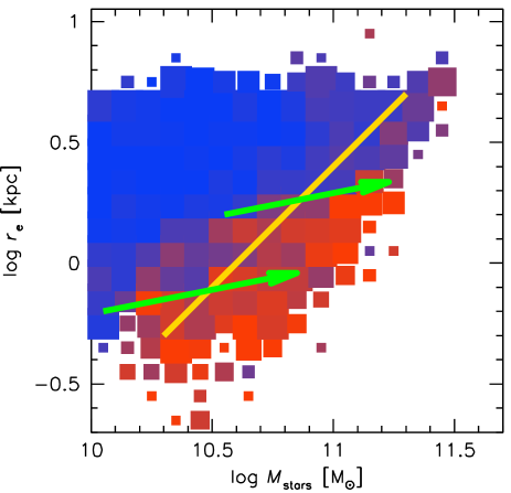
Figure 24.— Illustration of the “parallel track” model of massive galaxy evolution. The blue and red squares show the distribution of galaxies in the size-mass plane at $1.5<z<2.25$, with the size of the square proportional to the number of galaxies and the color indicating the fraction of quiescent galaxies. Galaxies move along parallel tracks in the size-mass plane, with $\Delta\log r_{\rm e}\sim 0.3\Delta\log M_{\rm stars}$, until they cross the yellow quenching line of constant $\sigma_{\rm q}\sim 225$ km s^-1.

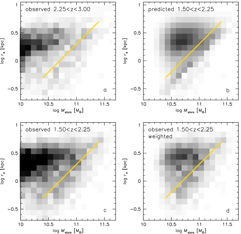
Figure 25.— Testing the “parallel track” model for the creation of compact massive galaxies. Panel (a) shows the observed number density of galaxies in the size-mass plane at $2.25<z<3.00$, with the grey scale proportional to the number of galaxies. In panel (b) the distribution is evolved forward in time by 1.0 Gyr to $1.50<z<2.25$, by assuming that galaxies grow along lines of $\Delta\log r_{e}=0.3\Delta\log M_{\rm stars}$ and quench after they pass the yellow line. Panel (c) shows the observed number density of galaxies at $1.50<z<2.25$. Panel (d) is identical to panel (c), but weighted to account for the edge effect at low masses in the model prediction of panel (b). The distribution of galaxies in panel (d) is remarkably similar to that in panel (b), demonstrating that compact massive galaxies at $z\sim 2$ can be formed by simple mass growth of galaxies at higher redshift.

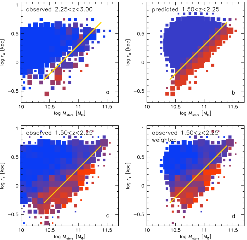
Figure 26.— Same as Fig. 25, but with color coding indicating the median specific star formation rate of the galaxies. Our simple model naturally produces a population of massive, compact quiescent galaxies at $M_{\rm stars}\sim 10^{11}$ $M_{\odot}$ and $r_{e}\sim 1$ kpc. The model overpredicts the quiescent fractions at the largest masses and sizes.

8.2. Testing the Model

We test the model in the following way. We first quantify the distribution of galaxies in the size-mass plane at $2.25<z<3.0$, by measuring the number of galaxies in bins of 0.1 dex $\times$ 0.1 dex (see Fig. 25a). Next, we evolve this distribution forward in time, using timesteps of $\Delta t=100$ Myr. For each combination of $(M_{\rm stars},r_{\rm e})$ we can calculate the SFR from Eq. 33, $P_{\rm q}$ from Eq. 31, the change in mass from Eq. 32, and the corresponding change in size from Eq. 30.

The evolved distribution after 10 timesteps (i.e., 1 Gyr) is shown in Fig. 25b, with a small (4 %) correction to account for the volume difference between $2.25<z<3.00$ and $1.50<z<2.25$. As expected, the galaxies have shifted to larger masses and to slightly larger radii in the size-mass plane. The distribution artificially falls off at low masses due to the $M_{\rm stars}=10^{10}$ $M_{\odot}$ limit in Fig. 25a. This limit was chosen to ensure that the galaxies with the lowest masses and highest redshifts have robust size measurements: the median brightness of the 28 galaxies with $10.0<\log M_{\rm stars}<10.1$ and $2.9<z<3.0$ is $\langle H_{160}\rangle=23.9$, well within the regime where size measurements are reliable (see van der Wel et al. 2014b).

The observed distribution of galaxies at $1.50<z<2.25$ is shown in Fig. 25c. In panel (d) this observed distribution is multiplied by a weight mask, to account for the artificial fall-off at low masses in panel (b). The weight mask was constructed by evolving a galaxy population with a uniform density distribution in the size-mass plane and a cutoff at $M_{\rm stars}<10^{10}$ $M_{\odot}$ forward in time (in the same way as described above). The distribution in Fig. 25d is remarkably similar to that in Fig. 25b. Furthermore, the total number density of galaxies in the two panels is almost identical; panel (d) has 7 % less galaxies than panel (b).

In Fig. 26 the color-coding reflects the specific star formation rates of the galaxies, with redder squares indicating a lower SSFR. The figure looks very similar when the fraction of quiescent galaxies is used for the color coding instead of the SSFR. The sizes of the squares are proportional to the number of galaxies. The model naturally produces a population of quiescent galaxies with $M_{\rm stars}\sim 10^{11}$ $M_{\odot}$ and $r_{e}\sim 1$ kpc. In our model, the progenitors of these galaxies have masses of $\sim 3\times 10^{10}$ $M_{\odot}$ and sizes of $\sim 0.7$ kpc at $z\sim 3$. The model does not produce the right fraction of quiescent galaxies at the highest masses and largest sizes: many of these galaxies are forming stars at $z\sim 1.9$ even though they have high galaxy-averaged velocity dispersions. This suggests that our quenching prescription is too simplistic in this regime (see Sect. 8.3).

We compare the predicted to the observed number densities explicitly in Fig. 27. This Figure highlights the excellent match of our model to the size distribution of all galaxies over the entire mass range $10.5<\log M_{\rm stars}<11.5$: it not only reproduces the peak in the distribution at $r_{e}\sim 2.5$ kpc but also the “shoulder” of compact quiescent galaxies. It also demonstrates that the modeling of quenching is too simplistic for large galaxies, as was already clear from the comparison of panels (b) and (d) of Fig. 26. In particular, nearly 100 % of galaxies with $r_{e}>2$ kpc are forming stars in the model, whereas the observed star forming fraction is only $\sim 85$ %.

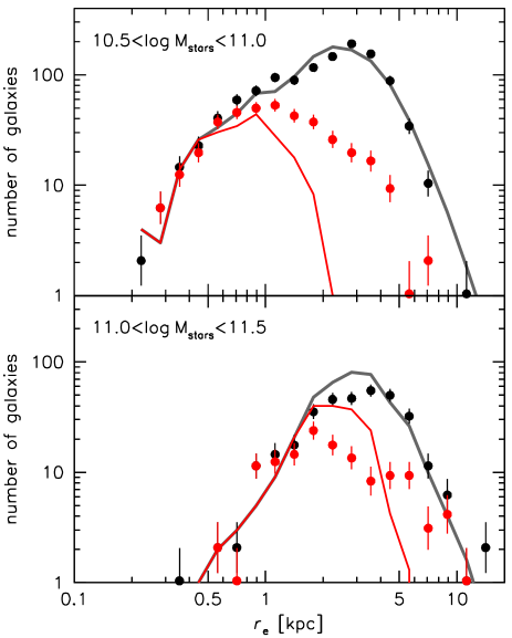
Figure 27.— The number density of galaxies as a function of size at $1.50<z<2.25$, in two mass bins. Points with errorbars are the observed values; black points show all galaxies and red points show quiescent galaxies only. The lines are the predicted distributions in our model, that is, the observed distribution at $2.25<z<3.00$ evolved forward in time by 1.0 Gyr. The size distributions are well reproduced in this model, in both mass bins (black lines). The match to the subset of quiescent galaxies is very good at the smallest sizes but shows systematic differences at intermediate and large sizes.

8.3. Summary of the Modeling

In summary, we have shown that the population of compact, massive galaxies at $z\sim 2$ can be explained by a model in which galaxies form stars at a rate that is dictated by the star forming sequence, experience a modest increase in size for a given increase in mass, and quench after passing a velocity dispersion threshold. This was demonstrated by evolving the observed galaxy population at $z\sim 2.6$ forward by 1 Gyr to $z\sim 1.9$. This is a critical period as the number density of qCMGs increases by an order of magnitude over that redshift range.

Although it is beyond the scope of this (already somewhat unwieldy) paper, we note that the modeling can easily be extended. In particular, it would be straightforward to fit for the two tunable parameters (the quenching dispersion $\sigma_{q}$ and the parameter $\beta$, which relates the mass growth to the star formation rate). Furthermore, our quenching description is inadequate in the high mass / large size regime; the yellow line in Fig. 24 is somewhat too steep. A possible explanation is that quenching depends on the galaxy properties in the central $\sim 1$ kpc, and the simple $M_{\rm stars}/r_{e}$ criterion no longer “works” in a regime where $r_{e}\gg 1$ kpc. Some evidence for this comes from a study of the mass in the central $r_{\rm 3D}<1$ kpc of galaxies (van Dokkum et al. 2014): as we showed in Fig. 9 of that paper the mass inside of 1 kpc is an excellent predictor of quiescence at all redshifts. Finally, the modeling can be extended to lower redshifts, taking evolution in $\sigma_{q}$ into account (see Sect. 9.1).

9. Discussion

9.1. The Formation of Today’s Massive Galaxies

In the preceding sections we discussed a simple model for the evolution of massive galaxies at $2<z<3$: they grow inside-out with $\Delta\log r_{\rm e}\sim 0.3\Delta\log M_{\rm stars}$ (Eq. 30) while they are forming stars, and quench when they reach a density or velocity dispersion threshold. This model provides an explanation for the fact that large galaxies have younger stellar populations than small galaxies at fixed mass (e.g., Franx et al. 2008), as only the smallest galaxies have reached the quenching threshold. Galaxies enter the massive, compact selection region in the size-mass plane “from the left”, that is, by increasing their masses. This seems different from models in which large, massive galaxies enter this region “from above”, that is, by decreasing their sizes through mergers (e.g., Hopkins et al. 2009b) or by gas “compaction” followed by star formation (Dekel & Burkert 2014). This apparent difference may reflect a difference in approach: in this paper we are concerned with the average evolution of the population of massive galaxies, whereas simulations such as those of Zolotov et al. (2015) are able to follow the tracks of individual galaxies in the size-mass plane. Judging from the Zolotov et al. (2015) tracks, Eq. 30 may simply be the time- and population average of periods of proportional size and mass growth ($\Delta\log r_{\rm e}\sim\Delta\log M_{\rm stars}$), periods of compaction, and the effects of mergers.

At lower redshifts massive galaxies evolve along a markedly different track in the size-mass plane: van Dokkum et al. (2010), Patel et al. (2013), and others find that the size and mass evolution of massive galaxies are related through $\Delta\log r_{\rm e}\sim 2\Delta\log M_{\rm stars}$ at $0<z<2$ (as indicated by the dotted section of the red curve in Fig. 22). This evolution can be explained by minor, gas-poor mergers building up the outer envelopes of galaxies (Bezanson et al. 2009; Naab et al. 2009; Hopkins et al. 2010; Hilz et al. 2013). In van Dokkum et al. (2010) we showed that any physical process that deposits mass at $r>r_{\rm e}$ leads to a steep track in the size-mass plane, due to the definition of the effective radius.

A schematic of the growth of massive galaxies from $z\sim 3$ to $z\sim 0$ is shown in Fig. 28. After galaxies quench, their mass growth per unit time is reduced, but their effective radii continue to increase. This Figure suggests that there are multiple paths leading to large, massive, quiescent galaxies in the local Universe, as was also noted in, e.g., Cappellari et al. (2013) and Barro et al. (2014a). Their $z\sim 2$ progenitors can be large star forming (disk) galaxies, such as those studied extensively by, e.g., Genzel et al. (2008) and Förster Schreiber et al. (2011), or compact, massive, quiescent galaxies that have grown through mergers (e.g., Trujillo et al. 2011; Patel et al. 2013; Ownsworth et al. 2014). As shown in Fig. 2 of van Dokkum et al. (2014) massive $z=0$ galaxies have a large range of central densities at fixed total mass, as expected in such scenarios. It is possible that massive S0 galaxies formed from large star forming galaxies and massive elliptical galaxies formed from compact star forming galaxies, although it remains to be seen whether the stellar populations of massive early-type galaxies are sufficiently diverse to accommodate a large range in formation histories (Gallazzi et al. 2005; van Dokkum & van der Marel 2007).

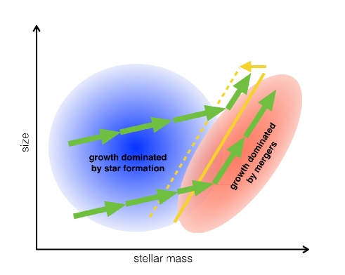
Figure 28.— Illustration of possible average tracks of galaxies in the size-mass plane from $z\sim 3$ to $z\sim 0$. While they are forming stars, galaxies grow mostly in mass and gradually increase their density. After reaching a velocity dispersion or stellar density threshold (the yellow line, whose location is redshift dependent) they quench, due to AGN feedback or other processes that correlate with stellar density. The dominant mode of growth after quenching is dry merging, which takes galaxies on a steep track in the size-mass plane.

9.2. Winds, Shocks, and AGN

In this paper we mostly ignored the effects of AGN, despite the fact that nearly half of the 25 galaxies with Keck spectra have X-ray luminosities above the canonical AGN limit of $L_{\rm X}>10^{43}$ ergs s^-1. The reason is that these effects are difficult to constrain and quantify. Barro et al. (2013) discuss the high occurrence rate of AGN in compact star forming galaxies extensively, and argue that they are the agent of quenching. This may be true: in many galaxy formation models AGNs play a crucial role in quenching star formation precisely in this mass and redshift range (e.g., Croton et al. 2006; Hopkins et al. 2008). However, the star formation rates of the sCMGs are (still) high and consistent with the $z\sim 2.3$ star forming sequence (Whitaker et al. 2014), and there is no evidence for a direct effect of the AGNs on star formation. Turning this around, it is obviously the case that the black holes are growing in these galaxies, and that they are growing at a time when the dense stellar centers are also growing. This is not surprising, as it is difficult to see how to avoid a high accretion rate onto the central object in these extremely dense, highly star forming galaxies.

An obvious point of concern is that the presence of AGNs causes errors in the derived physical parameters of the galaxies. In principle, an AGN in a relatively low mass, relatively large, and relatively quiescent galaxy could push the galaxy in the sCMG category: the extra light of the AGN could be mistaken for star light, increasing the mass; the combination of a point source with a normal galaxy could be mistaken for a compact bulge-dominated object; and the hot IR flux from the AGN could be mistaken for PAH features from star formation. This can only be addressed properly with data of much higher spatial resolution than is available today, but we note here that the galaxies with AGNs do not stand out in any of the figures. The only exception is that the four galaxies with the highest measured velocity dispersions all have X-ray AGN, and also [Nii]/H$\alpha$ ratios of $\sim 1$. We have treated these four galaxies in the same way as the others.

A related issue is the almost-certain presence of galactic-scale winds and outflows. Such winds can be driven by star formation (e.g., Heckman, Armus, & Miley 1987) and/or AGNs (e.g., Proga, Stone, & Kallman 2000) and are ubiquitous in star forming galaxies at high redshifts (Franx et al. 1997; Pettini et al. 1998; Förster Schreiber et al. 2014; Genzel et al. 2014a). Galactic superwinds can create bubbles and shock fronts whose kinematics, spatial extent, and emission line ratios are very similar to what we observe. In at least one of the galaxies in our sample, COSMOS_1014, there is evidence for a broad H$\alpha$ line in addition to a narrow component, similar to IRAS 11095–0238 (Soto & Martin 2012) and galaxies in Förster Schreiber et al. (2014). Furthermore, four of the galaxies in our sample are part of the sample of massive galaxies of Genzel et al. (2014a) (COSMOS_11363, GOODS-S_30274, GOODS-S_37745, and GOODS-S_45068), and they find broad nuclear velocity components in two of them (COSMOS_11363 and GOODS-S_30274). A detailed study of the kinematics and line ratios of GOODS-S_30274 was also done by van Dokkum et al. (2005).

Although winds are almost certainly present, two results suggest that they are not dominating the galaxy-integrated emission line widths. First, winds tend to escape in a direction perpendicular to the plane of the galaxy (Heckman, Armus, & Miley 1990), which is difficult to reconcile with the observed anti-correlation between velocity dispersion and axis ratio (Fig. 12). Second, the observed kinematics are fully explained by the stellar mass, leaving little room for additional broadening due to winds. In fact, broad components in the velocity profiles are expected just from rotating gas at small radii: as shown in Fig. 18 gas at $\sim 1$ kpc should have FWHM $\approx 1000$ km s^-1 even in the absense of winds. Judging from other $z\sim 2$ galaxies the disks are also likely to be highly turbulent, with a relatively high internal dispersion (see, e.g., Cresci et al. 2009; Förster Schreiber et al. 2009). The gaseous environments of sCMGs may be similar to those of ULIRGs, which are highly complex: as shown in Soto & Martin (2012) they can have rotating, large-scale disks in addition to outflows and shocks.

Finally, we note that the presence of spatially-extended gas disks in these galaxies had been predicted by Zolotov et al. (2015). They also predicted that the gas dispersions are, on average, lower than the stellar dispersions (Fig. 10a), as the gas is in disks which are sometimes seen face-on. Interestingly, Zolotov et al. (2015) also find that the gas constitutes only a small fraction of the total baryonic mass of the simulated compact massive star forming galaxies, although they note that this result is sensitive to the feedback prescription. Similarly, Johansson et al. (2012) predicted that compact, massive galaxies are stellar mass-dominated and have Keplerian rotation curves; the model rotation curves in their Fig. 7 are remarkably similar to the inferred rotation curve shown in our Fig. 18.

9.3. Submm-Galaxies, Far-IR Selected Galaxies, and Quasars

This study begins with an HST/WFC3-selected sample in a total area of $\sim 0.25$ square degrees. Many other studies have found extreme star forming galaxies by selecting them on the basis of their far-infrared, submm, or radio emission instead (e.g., Kormendy & Sanders 1992; Sanders & Mirabel 1996; Barger et al. 1998; Smail et al. 2000; Barger et al. 2001; Casey et al. 2012). These extreme galaxies are plausible ancestors of early-type galaxies; as an example, Tacconi et al. (2008), Toft et al. (2014), and Simpson et al. (2015) have suggested that many submm galaxies could be direct progenitors of compact quiescent galaxies at $z\sim 2$.

We do not select against such objects, and our sample should include the proper number of submm galaxies, radio galaxies, and other extreme objects. However, there are (at least) two possible reasons why galaxies selected at other wavelenghts could be underrepresented in our sample: some fraction may be too faint in the near-IR to be included (or to be properly characterized) in the Skelton et al. (2014) catalogs, and some may be too rare to be represented in the 3D-HST/CANDELS area. sCMGs have such high column densities in the central regions that some may be entirely obscured at rest-frame optical wavelengths (Gilli et al. 2014; Nelson et al. 2014). Wang, Barger, & Cowie (2012) and Caputi et al. (2014) show that objects exist that are relatively bright in the IRAC bands but that are undetected in deep near-IR data. It is obviously difficult to measure the redshifts and masses of these objects with traditional means, but it may be possible using molecular lines (see Walter et al. 2012; Riechers et al. 2013). In the context of the study presented here the question is not whether any massive, compact, “optically-dark” galaxies were missed, but what fraction of mass and star formation is in such objects.

The second class of potentially missed objects are extremely rare, extremely luminous galaxies. The median star formation rates of sCMGs in our study is $\langle{\rm SFR}\rangle=134$ $M_{\odot}$ yr^-1, and we have 112 such objects at $2<z<2.5$. Therefore, objects that are so rare that there are only a few (or zero) in our survey volume must have star formation rates $\gtrsim 5000$ $M_{\odot}$ yr^-1 to have a significant impact on our results. This seems extreme, but such objects probably exist: the most extreme Herschel-selected galaxies at $2<z<5$ have estimated star formation rates up to $\sim 9000$ $M_{\odot}$ yr^-1 (Casey et al. 2012). Furthermore, recently identified highly obscured quasars have bolometric luminosities of $L_{\rm bol}\sim 10^{47}$ ergs s^-1 (Banerji et al. 2012, 2015), and it seems likely that the growth of the black holes in these objects is accompanied by prodigious star formation. It remains to be seen whether such objects are sufficiently common (or rather, long-lived) to impact results derived from CANDELS-sized areas.

Finally, we note that we do not find a correlation between size and IR luminosity at fixed stellar mass, that is, an IR selection does not preferentially select compact galaxies but objects with a wide range of rest-frame optical sizes (see also Wiklind et al. 2014; Simpson et al. 2015). As an IR selection is effectively a star formation selection at high masses (see, e.g., Whitaker et al. 2012; Rodighiero et al. 2014), this is perhaps not surprising.

10. Summary and Conclusions

In this paper we have identified a population of star forming, compact, massive galaxies in the five fields of the CANDELS and 3D-HST surveys. Such objects have been studied previously by Barro et al. (2013, 2014b, 2014a) and Nelson et al. (2014), and we build on their results. Compared to the Barro et al. studies, our selection is more restrictive, focusing only on the most massive and most compact galaxies; we study an area that is $\sim 2.5$ times larger; and our redshift catalogs make use of the 3D-HST grism spectra for all objects brighter than $H_{160}<24$.

We first confirm the redshifts and masses of the galaxies using Keck MOSFIRE and NIRSPEC spectroscopy of 25 compact massive star forming galaxies at $2<z<2.5$. The gas dynamics suggest that the galaxies are embedded in spatially-extended rotating disks; this explains the low measured dispersions of a large fraction of the sample and the observed anti-correlation between the disperion and the axis ratio of the galaxies. Support for this interpretation comes from direct measurements of the sizes of the H$\alpha$ disks for 10 galaxies; the fact that this is possible at all from ground-based, seeing-limited data already shows that the gas extends to scales $\gg$ 1 kpc. The derived sizes of the gas disks, and the fall-off of the rotation curve that we construct for the galaxies, are in very good agreement with recent models for the formation of massive galaxies (Johansson et al. 2012; Zolotov et al. 2015).

It is important to note that, in our interpretation, the measured gas velocity dispersions of the galaxies generally do not reflect the true $V_{\rm rot}$ in the stellar body. We predict that the (inclination-corrected) velocities at $r\lesssim 1$ kpc are $400-500$ km s^-1for all galaxies. This can be tested with adaptive optics-assisted observations of the H$\alpha$ line. There is evidence for broad components in several of the velocity profiles (see Sect. 9.2), and these complex profiles may reflect the combined effect of high rotation velocities at small radii and lower velocities at larger radii. A more direct measurement could come from CO line widths, as these likely probe much smaller radii than the H$\alpha$ emission (see, e.g., Downes & Solomon 1998).

Next, we interpret the existence of star forming, compact galaxies at $2<z<2.5$ in the context of a simple model for the evolution of galaxies in the size-mass plane. We describe the average evolution of star-forming galaxies by the simple relation $\Delta\log r_{\rm e}\sim 0.3\Delta\log M_{\rm stars}$, with the mass evolution proportional to the main sequence star formation rate. We show that this evolution is a consistent feature in galaxy formation models of Hirschmann et al. (2013), Wellons et al. (2015), and Zolotov et al. (2015), and is also seen in observations of number density-matched samples of galaxies (van Dokkum et al. 2013; Patel et al. 2013; Ownsworth et al. 2014).

As galaxies move along this track their average 3D density within $r_{\rm e}$ remains approximately constant (as $\rho(r_{\rm e})\propto M/r_{\rm e}^{3}$, it follows that $r_{\rm e}\propto M^{1/3}$ if the density is constant). However, their density within a fixed physical radius increases, as does their projected (2D) density and their velocity dispersion. Following many other studies (e.g., Franx et al. 2008; Bell et al. 2012), we assume that quenching occurs when galaxies reach a threshold in either velocity dispersion or physical density. We show that this model explains the evolution of the distribution of galaxies in the size-mass plane from $z\sim 2.6$ to $z\sim 1.9$, the redshift range when the number density of massive compact quiescent galaxies increases by nearly an order of magnitude. In the context of this straightforward model, the progenitors of compact massive star forming galaxies at $z\sim 2.5$ were simply somewhat less massive and slightly smaller galaxies at $z\gtrsim 3$.

Our study has several important systematic uncertainties. First, the stellar masses of the galaxies are derived from fitting stellar population synthesis models to the photometry, and these models have not been tested for the extreme galaxies that are under discussion in this paper. Such tests are urgently needed but they are difficult, even for quiescent galaxies and for “normal” star forming galaxies in the local Universe (Muzzin et al. 2009b; Conroy 2013). One interpretation of Fig. 10b is that the stellar masses are off by factors up to $\sim 10$; however, as we show in the remainder of Sect. 5 the dynamical masses and stellar masses are consistent with each other once orientation effects and the spatial extent of the gas are taken into account. Our final dynamical result ($M_{\rm fit}=0.8^{0.6}_{-0.4}\times M_{\rm stars}$; Sect. 6.4) suggests that the contributions of dark matter and gas to the mass within $\sim 7$ kpc are small. We have assumed a relatively bottom-light Chabrier (2003) IMF when deriving stellar masses; if we assume a Salpeter (1955) IMF instead (see, e.g., van Dokkum & Conroy 2010; Conroy & van Dokkum 2012; Cappellari et al. 2012) we find $M_{\rm fit}=0.5^{+0.4}_{-0.2}\times M_{\rm stars}$, and even tighter constraints on the amount of gas and dark matter. We emphasize, however, that the conversion of light to stellar mass for these dusty, compact star forming galaxies is highly uncertain. We also note here that the stellar masses are not corrected for the contribution of emission lines to the SEDs. These corrections are generally small ($\sim 10$ %).

Second, the role of winds and active nuclei in these galaxies is not well understood (Sect. 9.2). They almost certainly influence the measured dynamics and line ratios, but without spatially-resolved data it is very difficult to disentangle the effects of winds, a falling rotation curve, and the spatial distribution of the ionized gas. Third, the fact that the galaxies are all very dusty may imply that we are missing part of the population due to selection effects (Sect. 9.3). We could be missing galaxies outright (see Fig. 3 in Nelson et al. 2014), or they could be misclassified as less compact, lower mass galaxies if only their outer edges are detected in the currently available data. Another potential effect of the dust is that the stellar population modeling may produce incorrect stellar masses: the modeling uses a screen approximation for dust, whereas in reality the dust and stars are almost certainly mixed.

Fortunately, the prospects for addressing these uncertainties are excellent. Adaptive optics-assisted spectroscopic observations with integral field units on 8 m – 10 m telescopes can be used to measure kinematics and line ratios on $\lesssim 1$ kpc scales (e.g., Newman et al. 2013). The morphology of the dust and molecular gas emission can be studied with interferometers such as the Very Large Array, the Plateau de Bure Interferometer, and the Atacama Large Millimeter Array (see, e.g., Simpson et al. 2015, for impressive early ALMA results on submm-selected galaxies). These instruments can also measure the kinematics of the molecular gas (e.g., Tacconi et al. 2008). On a longer timescale, the James Webb Space Telescope can measure the stellar kinematics of the galaxies, as well as identify and characterize compact galaxies that are entirely obscured in the $K$ band (Wang et al. 2012). Finally, the upcoming generation of extremely large ground-based optical/near-IR telescopes is needed to spatially resolve these compact, massive galaxies within their effective radius.

Appendix A A. $H_{160}$ Images

In the main text we show color images of the 25 star forming compact massive galaxies, created from the $J_{125}$ and $H_{160}$ CANDELS data (Fig. 6). In Fig. 29 we show the $H_{160}$ images separately, with a higher dynamic range than in Fig. 6. The tidal features around GOODS-S_30274 and COSMOS_11363 are very clear, and several other galaxies also show structure at faint surface brightness. We fit all galaxies with a single Sersic profile, which is an excellent approximation of the average surface brightness profile of the full sample (see Sect. 7.2); however, it is clear that these fits do not capture the full information in the HST images.

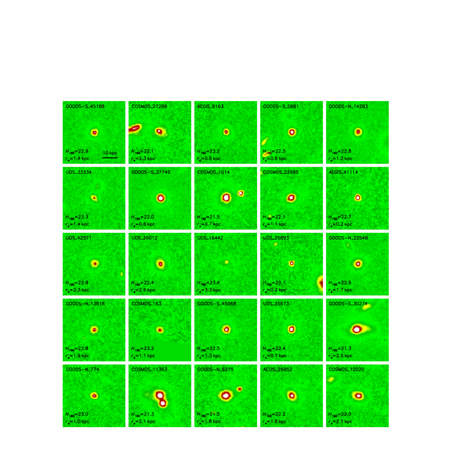
Figure 29.— HST images of the galaxies in Figs. 5, 6, 7, and 15, in the $H_{160}$ band. The galaxies are displayed with a high dynamic range, so that faint structures around bright cores can be seen more clearly than in Fig. 6 of the main text. GOODS-S_3027 4 and COSMOS_11363 show clear tidal features.

Appendix B B. Expected and Observed Uncertainties in the Spectra

As described in Sect. 3.4.1 we fit Gaussian models to the emission lines. The fits are done with the emcee code, with the observed 1D spectrum and a noise model as inputs for each galaxy. Here we briefly analyze the residuals from these fits to determine the accuracy of the noise models.

In Fig. 30 we show the spectra of the 20 galaxies that were observed by us. For convenience, the figure has the same format as Figs. 5, 6, 7, and 15 in the main text, except that the five galaxies from Barro et al. (2014) are left blank. For each galaxy three subpanels are shown. The top subpanel is identical to the main panel of Fig. 5, and shows the observed spectrum in black along with the best-fitting model in red. The middle subpanel shows the noise model (empirical in the case of MOSFIRE and theoretical in the case of NIRSPEC; see Sect. 3.1 and Sect. 3.2). The bottom subpanel is the residual from the fit divided by the noise model.

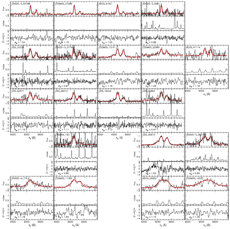
Figure 30.— Analysis of the noise in the NIRSPEC and MOSFIRE spectra. The galaxies have the same order as in Fig. 5; panels for objects taken from Barro et al. (2014) are left blank. For each galaxy, the top panel shows the spectrum and the best-fitting model; the middle panel shows the expected noise (see Sect. 3.1 and Sect. 3.2); and the bottom panel shows the difference between the observed spectrum and the best-fitting model divided by the expected noise. The width of the distribution of these residuals is $\sim 1$ in nearly all cases.

The residuals are well-behaved, and generally exhibit no indications of poorly subtracted sky lines or other irregularities. We quantified this by calculating the biweight scatter $\sigma_{\rm BI}$ (see Beers et al. 1990) in the distribution of residuals. The value of $\sigma_{\rm BI}$ deviates by more than $\sim 30$ % from unity in only two cases, UDS_35673 and COSMOS_11363. Both galaxies have very high S/N ratio spectra, and the higher than expected residuals are not caused by errors in the noise spectra but by the fact that the velocity distributions are not exactly Gaussian. The average scatter of the remaining 18 galaxies is $\langle\sigma_{\rm BI}\rangle=1.09$, which means that the noise models that we use are accurate to $\sim 10$ %.

Appendix C C. Converting Galaxy-Averaged Velocity Dispersions to a Rotation Curve

C.1. Motivation

In Sect. 6.4 we construct the average rotation curve for star forming compact massive galaxies. This is done by combining information for 10 different galaxies: all galaxies have approximately the same stellar masses and $H_{160}$ half-light radii, but they have a wide range of H$\alpha$ effective radii. For each galaxy we measure the galaxy-integrated velocity dispersion and the inclination, and convert these to an inclination-corrected rotation velocity at $r=r_{\rm gas}$, where $r_{\rm gas}$ is the half-light radius of the H$\alpha$ emission. The rotation velocities of the galaxies are then plotted versus $r_{\rm gas}$ in Fig. 18, and the resulting relation is interpreted as a rotation curve.

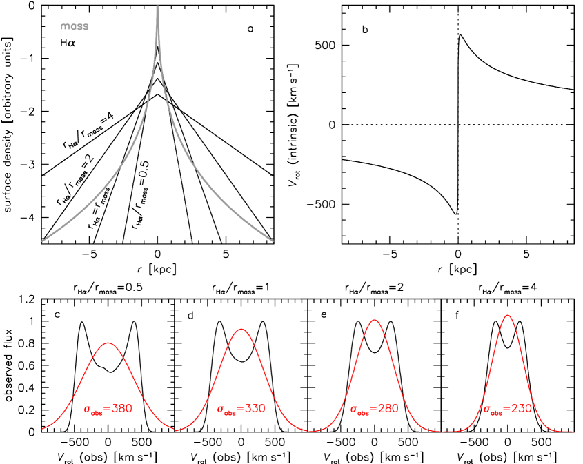
Figure 31.— a) Surface density profile of a model galaxy with a stellar mass of $10^{11}$ $M_{\odot}$, Sersic index $n=4$, and an effective radius $r_{\rm mass}=1$ kpc (grey). Black lines show four different H$\alpha$ $n=1$ surface brightness profiles, with effective radii ranging from 0.5 kpc to 4 kpc. b) Rotation curve of the H$\alpha$-emitting gas disks in the model galaxy. The H$\alpha$ emission is assumed to be a tracer, not a contributor, to the mass, and the rotation curve is identical in all four models. c-f) Observed galaxy-integrated H$\alpha$ velocity profiles for the four surface brightness profiles shown in panel a, assuming an inclination of 60$\arcdeg$ and an instrumental resolution of 60 km s^-1. The red curves are Gaussian fits to the observed profiles. The measured dispersion is lower for higher values of $r_{{\rm H}\alpha}/r_{\rm mass}$, as the profile is weighted toward larger radii.

Here we test whether this method is viable, that is, whether the actual rotation curve of a model galaxy can be reconstructed in this way. We also test whether we are using the correct conversion constant to go from a galaxy-integrated velocity dispersion to a rotation velocity at the half-light radius of H$\alpha$. This constant, together with an inclination correction, relates the velocity dispersion $\sigma$ to the rotation velocity $V_{\rm rot}$:

$$\alpha=\frac{\sigma_{\rm gas}}{V_{\rm rot}\sin^{-1}(i)}$$ (C1)

(see Eq. 17 and Eq. 19). In the main text we use $\alpha=0.8\pm 0.2$, based on previous studies (see Sect. 5.1). However, these studies did not consider the specific model of a compact, $r^{1/4}$-law mass distribution combined with an extended, exponential gas distribution.

C.2. Modeling Velocity Profiles

We simulated the observations in the following way. We constructed a model mass distribution that follows a Sersic surface density profile. This mass distribution is characterized by three parameters: the Sersic index $n$, the effective radius $r_{\rm mass}$ (this parameter is equivalent to both $r_{\rm stars}$ and $r_{e}$ in the main text), and the total mass $M$. We fixed $r_{\rm mass}=1$ kpc and $M=1.0\times 10^{11}$ $M_{\odot}$, and for the initial model we set $n=4$. Apart from a slight rescaling of the effective radius, this model closely matches the actual average stellar mass distribution of the sCMGs, if mass traces the $H_{160}$ light. The model is shown in Fig. 31a by the grey line.

Next, we constructed 10 model galaxies, each with the same mass distribution but with different distributions of the H$\alpha$ emission. The ionized gas is in thin exponential disks, with effective radii ranging from $r_{{\rm H}\alpha}=0.5$ kpc (and hence $r_{{\rm H}\alpha}=0.5r_{\rm mass}$) to $r_{{\rm H}\alpha}=5$ kpc. Four of these model gas distributions are shown by the black lines in Fig. 31a. The gas disks mimic the derived extended ionized gas of sCMGs, with $r_{{\rm H}\alpha}$ equivalent to the parameter $r_{\rm gas}$ in the main text. Galaxy-integrated velocity profiles were created by integrating the projected velocities along the line of sight and over the full spatial extent of the model galaxies. The velocities were calculated from the mass profile shown in Fig. 31a and weighted by the H$\alpha$ flux. In order to model the observed profiles as closely as possible, we used an inclination of 60$\arcdeg$ (where $90\arcdeg$ is edge-on) and an instrumental resolution of 60 km s^-1 (in between the MOSFIRE and NIRSPEC resolution).

The velocity profiles of the four model galaxies are shown in panels c-f of Fig. 31. As expected they have the classic “double-horned” form that is characteristic of rotating disks. The profile is not the same for all four models even though the mass distribution, and hence the underlying velocity field, is identical in all cases. The more extended the H$\alpha$ distribution is with respect to the mass, the narrower the profile becomes, and the more closely it resembles a Gaussian. The reason for this behavior is that the H$\alpha$ emission is more weighted toward larger radii, where the rotation velocity is lower. Velocities in excess of $\sim 350$ km s^-1 are still sampled, but they have relatively low weight and are responsible for the high velocity tails of the profile.

C.3. Relation Between Global Dispersion and Rotation Velocity at $r=r_{{\rm H}\alpha}$

We fitted Gaussian models to the line profiles, just as we do in the data analysis described in the main text. These Gaussian fits are shown by the red curves in panels c-f of Fig. 31. The width of these Gaussians decreases with increasing $r_{{\rm H}\alpha}/r_{\rm mass}$, as discussed above. We note here that the actual profile shape is not very well approximated by a Gaussian, particular in panels c and d. Interestingly, we see hints of double-horned profiles in the data for some of the galaxies (e.g., UDS_16442 and, particularly, GOODS-N_774, which was published in Nelson et al. 2014), although the S/N ratio is not high enough to quantify this.

In Fig. 32a these measured galaxy-integrated velocity dispersions are plotted versus the half-light radii of the H$\alpha$ disks, after correcting for inclination and instrumental broadening (open squares). All ten galaxy models are shown, with H$\alpha$ effective radii ranging from $0.5\times r_{\rm mass}$ to $5\times r_{\rm mass}$. For comparison, the black curve shows the actual rotation curve of the galaxies. The squares show the same fall-off as the actual rotation curve, with a roughly constant multiplicitative offset. The solid squares are obtained by dividing the measured dispersions by 0.8, which is the value of $\alpha=\sigma/V_{\rm rot}$ that we used in the analysis of Sect. 6.4. They are in almost perfect agreement with the black curve, demonstrating that it is possible to reconstruct the average rotation curve of sCMGs with our method.

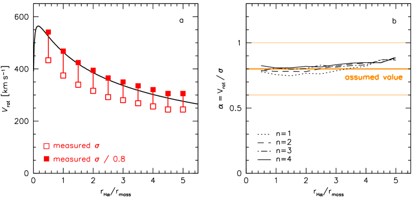
Figure 32.— a) Rotation curve of the model in Fig. 31 (black line), compared to the inclination-corrected, galaxy-integrated velocity dispersion $\sigma$ for 10 different H$\alpha$ distributions (open red squares). The half-light radius of the H$\alpha$ emission ranges from $0.5\times r_{\rm mass}$ to $5\times r_{\rm mass}$. Solid red squares are corrected for the parameter $\alpha=\sigma/V_{\rm rot}=0.8$. b) Derived values of $\alpha$ from our model (black lines). The value $\alpha=0.8\pm 0.2$ that is used in the main text is shown by the orange line. Different line types indicate results for different Sersic indices $n$ of the mass distribution; the value of $\alpha$ is nearly independent of $n$.

The analysis is generalized in Fig. 32b, where we show the value of $\alpha$ as a function of the ratio of the effective radius of H$\alpha$ and the effective radius of the mass. We repeated the analysis for different assumed mass profiles, ranging from exponential ($n=1$; dotted) to an $r^{1/4}$ law ($n=4$; solid). The ratio between dispersion and rotation velocity at $r=r_{{\rm H}\alpha}/r_{\rm mass}$ is remarkably constant: it does not vary appreciably either with $r$ or with $n$. We conclude that the assumed value of $\alpha=0.8\pm 0.2$ is reasonable for the mass and H$\alpha$ profiles discussed in this paper.

References

- (1)
- (2) Alonso-Herrero, A., García-Marín, M., Rodríguez Zaurín, J., Monreal-Ibero, A., Colina, L., & Arribas, S. 2010, A&A, 522, A7
- (3)
- (4) Baldwin, J. A., Phillips, M. M., & Terlevich, R. 1981, PASP, 93, 5
- (5)
- (6) Banerji, M., Alaghband-Zadeh, S., Hewett, P. C., & McMahon, R. G. 2015, MNRAS, 447, 3368
- (7)
- (8) Banerji, M., McMahon, R. G., Hewett, P. C., Alaghband-Zadeh, S., Gonzalez-Solares, E., Venemans, B. P., & Hawthorn, M. J. 2012, MNRAS, 427, 2275
- (9)
- (10) Barden, M., Häußler, B., Peng, C. Y., McIntosh, D. H., & Guo, Y. 2012, MNRAS, 422, 449
- (11)
- (12) Barger, A. J., Cowie, L. L., Mushotzky, R. F., & Richards, E. A. 2001, AJ, 121, 662
- (13)
- (14) Barger, A. J., Cowie, L. L., Sanders, D. B., Fulton, E., Taniguchi, Y., Sato, Y., Kawara, K., & Okuda, H. 1998, Nature, 394, 248
- (15)
- (16) Barro, G., Faber, S. M., Pérez-González, P. G., Koo, D. C., Williams, C. C., Kocevski, D. D., Trump, J. R., Mozena, M., et al. 2013, ApJ, 765, 104
- (17)
- (18) Barro, G., Faber, S. M., Pérez-González, P. G., Pacifici, C., Trump, J. R., Koo, D. C., Wuyts, S., Guo, Y., et al. 2014a, ApJ, 791, 52
- (19)
- (20) Barro, G., Trump, J. R., Koo, D. C., Dekel, A., Kassin, S. A., Kocevski, D. D., Faber, S. M., van der Wel, A., et al. 2014b, ApJ, 795, 145
- (21)
- (22) Beers, T. C., Flynn, K., & Gebhardt, K. 1990, AJ, 100, 32
- (23)
- (24) Behroozi, P. S., Marchesini, D., Wechsler, R. H., Muzzin, A., Papovich, C., & Stefanon, M. 2013, ApJ, 777, L10
- (25)
- (26) Bell, E. F., van der Wel, A., Papovich, C., Kocevski, D., Lotz, J., McIntosh, D. H., Kartaltepe, J., Faber, S. M., et al. 2012, ApJ, 753, 167
- (27)
- (28) Belli, S., Newman, A. B., & Ellis, R. S. 2014a, ApJ, 783, 117
- (29)
- (30) Belli, S., Newman, A. B., Ellis, R. S., & Konidaris, N. P. 2014b, ApJ, 788, L29
- (31)
- (32) Bertin, E. & Arnouts, S. 1996, A&AS, 117, 393
- (33)
- (34) Bezanson, R., Franx, M., & van Dokkum, P. G. 2015, ApJ, 799, 148
- (35)
- (36) Bezanson, R., van Dokkum, P. G., Franx, M., Brammer, G. B., Brinchmann, J., Kriek, M., Labbé, I., Quadri, R. F., et al. 2011, ApJ, 737, L31+
- (37)
- (38) Bezanson, R., van Dokkum, P. G., Tal, T., Marchesini, D., Kriek, M., Franx, M., & Coppi, P. 2009, ApJ, 697, 1290
- (39)
- (40) Bezanson, R., van Dokkum, P. G., van de Sande, J., Franx, M., Leja, J., & Kriek, M. 2013, ApJ, 779, L21
- (41)
- (42) Brammer, G. B., Sánchez-Janssen, R., Labbé, I., da Cunha, E., Erb, D. K., Franx, M., Fumagalli, M., Lundgren, B., et al. 2012a, ApJ, 758, L17
- (43)
- (44) Brammer, G. B., van Dokkum, P. G., & Coppi, P. 2008, ApJ, 686, 1503
- (45)
- (46) Brammer, G. B., van Dokkum, P. G., Franx, M., Fumagalli, M., Patel, S., Rix, H.-W., Skelton, R. E., Kriek, M., et al. 2012b, ApJS, 200, 13
- (47)
- (48) Brammer, G. B., Whitaker, K. E., van Dokkum, P. G., Marchesini, D., Franx, M., Kriek, M., Labbe, I., Lee, K.-S., et al. 2011, ApJ, 739, 24
- (49)
- (50) Brinchmann, J., Pettini, M., & Charlot, S. 2008, MNRAS, 385, 769
- (51)
- (52) Bruce, V. A., Dunlop, J. S., McLure, R. J., Cirasuolo, M., Buitrago, F., Bowler, R. A. A., Targett, T. A., Bell, E. F., et al. 2014, MNRAS, 444, 1660
- (53)
- (54) Calzetti, D., Armus, L., Bohlin, R. C., Kinney, A. L., Koornneef, J., & Storchi-Bergmann, T. 2000, ApJ, 533, 682
- (55)
- (56) Cappellari, M., Bacon, R., Bureau, M., Damen, M. C., Davies, R. L., de Zeeuw, P. T., Emsellem, E., Falcón-Barroso, J., et al. 2006, MNRAS, 366, 1126
- (57)
- (58) Cappellari, M., McDermid, R. M., Alatalo, K., Blitz, L., Bois, M., Bournaud, F., Bureau, M., Crocker, A. F., et al. 2012, Nature, 484, 485
- (59)
- (60) Cappellari, M., McDermid, R. M., Alatalo, K., Blitz, L., Bois, M., Bournaud, F., Bureau, M., Crocker, A. F., et al. 2013, MNRAS, 432, 1862
- (61)
- (62) Caputi, K. I., Michałowski, M. J., Krips, M., Geach, J. E., Ashby, M. L. N., Huang, J.-S., Fazio, G. G., Koekemoer, A. M., et al. 2014, ApJ, 788, 126
- (63)
- (64) Carollo, C. M., Bschorr, T. J., Renzini, A., Lilly, S. J., Capak, P., Cibinel, A., Ilbert, O., Onodera, M., et al. 2013, ApJ, 773, 112
- (65)
- (66) Casey, C. M., Berta, S., Béthermin, M., Bock, J., Bridge, C., Burgarella, D., Chapin, E., Chapman, S. C., et al. 2012, ApJ, 761, 139
- (67)
- (68) Cassata, P., Giavalisco, M., Guo, Y., Renzini, A., Ferguson, H., Koekemoer, A. M., Salimbeni, S., Scarlata, C., et al. 2011, ApJ, 743, 96
- (69)
- (70) Cassata, P., Giavalisco, M., Williams, C. C., Guo, Y., Lee, B., Renzini, A., Ferguson, H., Faber, S. F., et al. 2013, ApJ, 775, 106
- (71)
- (72) Chabrier, G. 2003, PASP, 115, 763
- (73)
- (74) Chang, Y.-Y., van der Wel, A., Rix, H.-W., Holden, B., Bell, E. F., McGrath, E. J., Wuyts, S., Häussler, B., et al. 2013, ApJ, 773, 149
- (75)
- (76) Conroy, C. 2013, ARA&A, 51, 393
- (77)
- (78) Conroy, C., van Dokkum, P., & Kravtsov, A. 2015, ApJ, 803, 77
- (79)
- (80) Conroy, C. & van Dokkum, P. G. 2012, ApJ, 760, 71
- (81)
- (82) Conselice, C. 2014, ARA&A, 52, 291
- (83)
- (84) Cresci, G., Hicks, E. K. S., Genzel, R., Förster Schreiber, N. M., Davies, R., Bouché, N., Buschkamp, P., et al. 2009, ApJ, 697, 115
- (85)
- (86) Croton, D. J., Springel, V., White, S. D. M., De Lucia, G., Frenk, C. S., Gao, L., Jenkins, A., Kauffmann, G., et al. 2006, MNRAS, 365, 11
- (87)
- (88) Daddi, E., Alexander, D. M., Dickinson, M., Gilli, R., Renzini, A., Elbaz, D., Cimatti, A., Chary, R., et al. 2007, ApJ, 670, 173
- (89)
- (90) Daddi, E., Bournaud, F., Walter, F., Dannerbauer, H., Carilli, C. L., Dickinson, M., Elbaz, D., Morrison, G. E., et al. 2010, ApJ, 713, 686
- (91)
- (92) Daddi, E., Renzini, A., Pirzkal, N., Cimatti, A., Malhotra, S., Stiavelli, M., Xu, C., Pasquali, A., et al. 2005, ApJ, 626, 680
- (93)
- (94) Damjanov, I., Abraham, R. G., Glazebrook, K., McCarthy, P. J., Caris, E., Carlberg, R. G., Chen, H.-W., Crampton, D., et al. 2011, ApJ, 739, L44
- (95)
- (96) Davari, R., Ho, L. C., Peng, C. Y., & Huang, S. 2014, ApJ, 787, 69
- (97)
- (98) Dekel, A., Birnboim, Y., Engel, G., Freundlich, J., Goerdt, T., Mumcuoglu, M., Neistein, E., Pichon, C., et al. 2009, Nature, 457, 451
- (99)
- (100) Dekel, A. & Burkert, A. 2014, MNRAS, 438, 1870
- (101)
- (102) Denicoló, G., Terlevich, R., & Terlevich, E. 2002, MNRAS, 330, 69
- (103)
- (104) Dopita, M. A. & Sutherland, R. S. 1995, ApJ, 455, 468
- (105)
- (106) Downes, D. & Solomon, P. M. 1998, ApJ, 507, 615
- (107)
- (108) Elbaz, D., Dickinson, M., Hwang, H. S., Díaz-Santos, T., Magdis, G., Magnelli, B., Le Borgne, D., Galliano, F., et al. 2011, A&A, 533, A119
- (109)
- (110) Erb, D. K., Shapley, A. E., Steidel, C. C., Pettini, M., Adelberger, K. L., Hunt, M. P., Moorwood, A. F. M., & Cuby, J. 2003, ApJ, 591, 101
- (111)
- (112) Fiore, F., Grazian, A., Santini, P., Puccetti, S., Brusa, M., Feruglio, C., Fontana, A., Giallongo, E., et al. 2008, ApJ, 672, 94
- (113)
- (114) Foreman-Mackey, D., Hogg, D. W., Lang, D., & Goodman, J. 2013, PASP, 125, 306
- (115)
- (116) Förster Schreiber, N. M., Genzel, R., Bouché, N., Cresci, G., Davies, R., Buschkamp, P., Shapiro, K., Tacconi, L. J., et al. 2009, ApJ, 706, 1364
- (117)
- (118) Förster Schreiber, N. M., Genzel, R., Newman, S. F., Kurk, J. D., Lutz, D., Tacconi, L. J., Wuyts, S., Bandara, K., et al. 2014, ApJ, 787, 38
- (119)
- (120) Förster Schreiber, N. M., Shapley, A. E., Erb, D. K., Genzel, R., Steidel, C. C., Bouché, N., Cresci, G., & Davies, R. 2011, ApJ, 731, 65
- (121)
- (122) Franx, M. 1993, in IAU Symposium, Vol. 153, Galactic Bulges, ed. H. Dejonghe & H. J. Habing, 243
- (123)
- (124) Franx, M., Illingworth, G., & de Zeeuw, T. 1991, ApJ, 383, 112
- (125)
- (126) Franx, M., Illingworth, G. D., Kelson, D. D., van Dokkum, P. G., & Tran, K. 1997, ApJ, 486, L75
- (127)
- (128) Franx, M., van Dokkum, P. G., Schreiber, N. M. F., Wuyts, S., Labbé, I., & Toft, S. 2008, ApJ, 688, 770
- (129)
- (130) Fumagalli, M., Patel, S. G., Franx, M., Brammer, G., van Dokkum, P., da Cunha, E., Kriek, M., Lundgren, B., et al. 2012, ApJ, 757, L22
- (131)
- (132) Fumagalli, M., Labbé, I., Patel, S. G., Franx, M., van Dokkum, P., Brammer, G., da Cunha, E., Förster Schreiber, N. M., et al. 2014, ApJ, 796, 35
- (133)
- (134) Gallazzi, A., Charlot, S., Brinchmann, J., White, S. D. M., & Tremonti, C. A. 2005, MNRAS, 362, 41
- (135)
- (136) Genel, S., Naab, T., Genzel, R., Förster Schreiber, N. M., Sternberg, A., Oser, L., Johansson, P. H., Davé, R., et al. 2012, ApJ, 745, 11
- (137)
- (138) Genzel, R., Burkert, A., Bouché, N., Cresci, G., Förster Schreiber, N. M., Shapley, A., Shapiro, K., Tacconi, L. J., et al. 2008, ApJ, 687, 59
- (139)
- (140) Genzel, R., Förster Schreiber, N. M., Rosario, D., Lang, P., Lutz, D., Wisnioski, E., Wuyts, E., Wuyts, S., et al. 2014a, ApJ, 796, 7
- (141)
- (142) Genzel, R., Förster Schreiber, N. M., Lang, P., Tacchella, S., Tacconi, L. J., Wuyts, S., Bandara, K., Burkert, A., et al. 2014b, ApJ, 785, 75
- (143)
- (144) Genzel, R., Tacconi, L. J., Gracia-Carpio, J., Sternberg, A., Cooper, M. C., Shapiro, K., Bolatto, A., Bouché, N., et al. 2010, MNRAS, 407, 2091
- (145)
- (146) Genzel, R., Tacconi, L. J., Lutz, D., Saintonge, A., Berta, S., Magnelli, B., Combes, F., García-Burillo, S., et al. 2015, ApJ, 800, 20
- (147)
- (148) Gilli, R., Norman, C., Vignali, C., Vanzella, E., Calura, F., Pozzi, F., Massardi, M., Mignano, A., et al. 2014, A&A, 562, A67
- (149)
- (150) Graham, A. W., Dullo, B. T., & Savorgnan, G. A. D. 2015, ApJ, 804, 32
- (151)
- (152) Grogin, N. A., Kocevski, D. D., Faber, S. M., Ferguson, H. C., Koekemoer, A. M., Riess, A. G., Acquaviva, V., Alexander, D. M., et al. 2011, ApJS, 197, 35
- (153)
- (154) Hammer, F., Flores, H., Puech, M., Yang, Y. B., Athanassoula, E., Rodrigues, M., & Delgado, R. 2009, A&A, 507, 1313
- (155)
- (156) Heckman, T. M., Armus, L., & Miley, G. K. 1987, AJ, 93, 276
- (157)
- (158) —. 1990, ApJS, 74, 833
- (159)
- (160) Hilz, M., Naab, T., & Ostriker, J. P. 2013, MNRAS, 429, 2924
- (161)
- (162) Hirschmann, M., Naab, T., Davé, R., Oppenheimer, B. D., Ostriker, J. P., Somerville, R. S., Oser, L., Genzel, R., et al. 2013, MNRAS, 436, 2929
- (163)
- (164) Hopkins, P. F., Bundy, K., Hernquist, L., Wuyts, S., & Cox, T. J. 2010, MNRAS, 401, 1099
- (165)
- (166) Hopkins, P. F., Bundy, K., Murray, N., Quataert, E., Lauer, T. R., & Ma, C.-P. 2009a, MNRAS, 398, 898
- (167)
- (168) Hopkins, P. F., Cox, T. J., Kereš, D., & Hernquist, L. 2008, ApJS, 175, 390
- (169)
- (170) Hopkins, P. F., Hernquist, L., Cox, T. J., Keres, D., & Wuyts, S. 2009b, ApJ, 691, 1424
- (171)
- (172) Johansson, P. H., Naab, T., & Ostriker, J. P. 2009, ApJ, 697, L38
- (173)
- (174) —. 2012, ApJ, 754, 115
- (175)
- (176) Kassin, S. A., Weiner, B. J., Faber, S. M., Gardner, J. P., Willmer, C. N. A., Coil, A. L., Cooper, M. C., Devriendt, J., et al. 2012, ApJ, 758, 106
- (177)
- (178) Kauffmann, G., Heckman, T. M., White, S. D. M., Charlot, S., Tremonti, C., Peng, E. W., Seibert, M., Brinkmann, J., et al. 2003, MNRAS, 341, 54
- (179)
- (180) Kennicutt, R. C. 1998, ARA&A, 36, 189
- (181)
- (182) Kewley, L. J., Dopita, M. A., Leitherer, C., Davé, R., Yuan, T., Allen, M., Groves, B., & Sutherland, R. 2013, ApJ, 774, 100
- (183)
- (184) Koekemoer, A. M., Faber, S. M., Ferguson, H. C., Grogin, N. A., Kocevski, D. D., Koo, D. C., Lai, K., Lotz, J. M., et al. 2011, ApJS, 197, 36
- (185)
- (186) Kormendy, J. & Sanders, D. B. 1992, ApJ, 390, L53
- (187)
- (188) Kriek, M., Shapley, A. E., Reddy, N. A., Siana, B., Coil, A. L., Mobasher, B., Freeman, W. R., de Groot, L., et al. 2015, ApJS, 218, 15
- (189)
- (190) Kriek, M., van Dokkum, P. G., Franx, M., Illingworth, G. D., Coppi, P., Förster Schreiber, N. M., Gawiser, E., Labbé, I., et al. 2007, ApJ, 669, 776
- (191)
- (192) Kriek, M., van Dokkum, P. G., Franx, M., Illingworth, G. D., & Magee, D. K. 2009a, ApJ, 705, L71
- (193)
- (194) Kriek, M., van Dokkum, P. G., Labbé, I., Franx, M., Illingworth, G. D., Marchesini, D., & Quadri, R. F. 2009b, ApJ, 700, 221
- (195)
- (196) Krist, J. 1995, in ASP Conf. Ser. 77: Astronomical Data Analysis Software and Systems IV, Vol. 4, 349
- (197)
- (198) Labbé, I., Huang, J., Franx, M., Rudnick, G., Barmby, P., Daddi, E., van Dokkum, P. G., Fazio, G. G., et al. 2005, ApJ, 624, L81
- (199)
- (200) Le Tiran, L., Lehnert, M. D., van Driel, W., Nesvadba, N. P. H., & Di Matteo, P. 2011, A&A, 534, L4
- (201)
- (202) Leja, J., van Dokkum, P., & Franx, M. 2013a, ApJ, 766, 33
- (203)
- (204) Leja, J., van Dokkum, P. G., Franx, M., & Whitaker, K. E. 2015, ApJ, 798, 115
- (205)
- (206) Leja, J., van Dokkum, P. G., Momcheva, I., Brammer, G., Skelton, R. E., Whitaker, K. E., Andrews, B. H., Franx, M., et al. 2013b, ApJ, 778, L24
- (207)
- (208) Magorrian, J., Tremaine, S., Richstone, D., Bender, R., Bower, G., Dressler, A., Faber, S. M., Gebhardt, K., et al. 1998, AJ, 115, 2285
- (209)
- (210) Marchesini, D., van Dokkum, P. G., Förster Schreiber, N. M., Franx, M., Labbé, I., & Wuyts, S. 2009, ApJ, 701, 1765
- (211)
- (212) Marsan, Z. C., Marchesini, D., Brammer, G. B., Stefanon, M., Muzzin, A., Fernández-Soto, A., Geier, S., Hainline, K. N., et al. 2015, ApJ, 801, 133
- (213)
- (214) McLean, I. S., Becklin, E. E., Bendiksen, O., Brims, G., Canfield, J., Figer, D. F., Graham, J. R., Hare, J., et al. 1998, in Society of Photo-Optical Instrumentation Engineers (SPIE) Conference Series, Vol. 3354, Infrared Astronomical Instrumentation, ed. A. M. Fowler, 566–578
- (215)
- (216) McLean, I. S., Steidel, C. C., Epps, H. W., Konidaris, N., Matthews, K. Y., Adkins, S., Aliado, T., Brims, G., et al. 2012, in Society of Photo-Optical Instrumentation Engineers (SPIE) Conference Series, Vol. 8446, Society of Photo-Optical Instrumentation Engineers (SPIE) Conference Series, 0
- (217)
- (218) Mentuch, E., Abraham, R. G., Glazebrook, K., McCarthy, P. J., Yan, H., O’Donnell, D. V., Le Borgne, D., Savaglio, S., et al. 2009, ApJ, 706, 1020
- (219)
- (220) Miller, S. H., Bundy, K., Sullivan, M., Ellis, R. S., & Treu, T. 2011, ApJ, 741, 115
- (221)
- (222) Mo, H. J., Mao, S., & White, S. D. M. 1998, MNRAS, 295, 319
- (223)
- (224) Moustakas, J. & Kennicutt, Jr., R. C. 2006, ApJS, 164, 81
- (225)
- (226) Muzzin, A., Marchesini, D., Stefanon, M., Franx, M., McCracken, H. J., Milvang-Jensen, B., Dunlop, J. S., Fynbo, J. P. U., et al. 2013, ApJ, 777, 18
- (227)
- (228) Muzzin, A., Marchesini, D., van Dokkum, P. G., Labbé, I., Kriek, M., & Franx, M. 2009a, ApJ, 701, 1839
- (229)
- (230) Muzzin, A., van Dokkum, P., Franx, M., Marchesini, D., Kriek, M., & Labbé, I. 2009b, ApJ, 706, L188
- (231)
- (232) Muzzin, A., van Dokkum, P., Kriek, M., Labbé, I., Cury, I., Marchesini, D., & Franx, M. 2010, ApJ, 725, 742
- (233)
- (234) Naab, T., Johansson, P. H., & Ostriker, J. P. 2009, ApJ, 699, L178
- (235)
- (236) Nelson, E., van Dokkum, P., Franx, M., Brammer, G., Momcheva, I., Schreiber, N. F., da Cunha, E., Tacconi, L., et al. 2014, Nature, 513, 394
- (237)
- (238) Nelson, E. J., van Dokkum, P. G., Brammer, G., Förster Schreiber, N., Franx, M., Fumagalli, M., Patel, S., Rix, H.-W., et al. 2012, ApJ, 747, L28
- (239)
- (240) Nelson, E. J., van Dokkum, P. G., Momcheva, I., Brammer, G., Lundgren, B., Skelton, R. E., Whitaker, K. E., Da Cunha, E., et al. 2013, ApJ, 763, L16
- (241)
- (242) Newman, A. B., Ellis, R. S., Bundy, K., & Treu, T. 2012, ApJ, 746, 162
- (243)
- (244) Newman, S. F., Genzel, R., Förster Schreiber, N. M., Shapiro Griffin, K., Mancini, C., Lilly, S. J., Renzini, A., Bouché, N., et al. 2013, ApJ, 767, 104
- (245)
- (246) Oesch, P. A., van Dokkum, P. G., Illingworth, G. D., Bouwens, R. J., Momcheva, I., Holden, B., Roberts-Borsani, G. W., Smit, R., et al. 2015, ApJ, 804, L30
- (247)
- (248) Oppenheimer, B. D. & Davé, R. 2006, MNRAS, 373, 1265
- (249)
- (250) Oser, L., Ostriker, J. P., Naab, T., Johansson, P. H., & Burkert, A. 2010, ApJ, 725, 2312
- (251)
- (252) Ownsworth, J. R., Conselice, C. J., Mortlock, A., Hartley, W. G., Almaini, O., Duncan, K., & Mundy, C. J. 2014, MNRAS, 445, 2198
- (253)
- (254) Papovich, C., Labbé, I., Quadri, R., Tilvi, V., Behroozi, P., Bell, E. F., Glazebrook, K., Spitler, L., et al. 2015, ApJ, 803, 26
- (255)
- (256) Papovich, C., Moustakas, L. A., Dickinson, M., Le Floc’h, E., Rieke, G. H., Daddi, E., Alexander, D. M., Bauer, F., et al. 2006, ApJ, 640, 92
- (257)
- (258) Patel, S. G., van Dokkum, P. G., Franx, M., Quadri, R. F., Muzzin, A., Marchesini, D., Williams, R. J., Holden, B. P., et al. 2013, ApJ, 766, 15
- (259)
- (260) Peng, C. Y., Ho, L. C., Impey, C. D., & Rix, H.-W. 2002, AJ, 124, 266
- (261)
- (262) Pettini, M., Kellogg, M., Steidel, C. C., Dickinson, M., Adelberger, K. L., & Giavalisco, M. 1998, ApJ, 508, 539
- (263)
- (264) Pettini, M. & Pagel, B. E. J. 2004, MNRAS, 348, L59
- (265)
- (266) Poggianti, B. M., Calvi, R., Bindoni, D., D’Onofrio, M., Moretti, A., Valentinuzzi, T., Fasano, G., Fritz, J., et al. 2013, ApJ, 762, 77
- (267)
- (268) Price, S. H., Kriek, M., Brammer, G. B., Conroy, C., Förster Schreiber, N. M., Franx, M., Fumagalli, M., Lundgren, B., et al. 2014, ApJ, 788, 86
- (269)
- (270) Proga, D., Stone, J. M., & Kallman, T. R. 2000, ApJ, 543, 686
- (271)
- (272) Reddy, N. A., Kriek, M., Shapley, A. E., Freeman, W. R., Siana, B., Coil, A. L., Mobasher, B., Price, S. H., et al. 2015, ApJ, 806, 259
- (273)
- (274) Riechers, D. A., Bradford, C. M., Clements, D. L., Dowell, C. D., Pérez-Fournon, I., Ivison, R. J., Bridge, C., Conley, A., et al. 2013, Nature, 496, 329
- (275)
- (276) Rix, H., Guhathakurta, P., Colless, M., & Ing, K. 1997, MNRAS, 285, 779
- (277)
- (278) Rodighiero, G., Renzini, A., Daddi, E., Baronchelli, I., Berta, S., Cresci, G., Franceschini, A., Gruppioni, C., et al. 2014, MNRAS, 443, 19
- (279)
- (280) Salpeter, E. E. 1955, ApJ, 121, 161
- (281)
- (282) Sanders, D. B. & Mirabel, I. F. 1996, ARA&A, 34, 749
- (283)
- (284) Scoville, N., Sheth, K., Aussel, H., Vanden Bout, P., Capak, P., Bongiorno, A., Casey, C. M., Murchikova, L., et al. 2015, ApJL, submitted (arXiv:1505.02159)
- (285)
- (286) Sersic, J. L. 1968, Atlas de galaxias australes (Cordoba, Argentina: Observatorio Astronomico, 1968)
- (287)
- (288) Shapley, A. E., Reddy, N. A., Kriek, M., Freeman, W. R., Sanders, R. L., Siana, B., Coil, A. L., Mobasher, B., et al. 2015, ApJ, 801, 88
- (289)
- (290) Simpson, J. M., Smail, I., Swinbank, A. M., Almaini, O., Blain, A. W., Bremer, M. N., Chapman, S. C., Chen, C.-C., et al. 2015, ApJ, 799, 81
- (291)
- (292) Skelton, R. E., Whitaker, K. E., Momcheva, I. G., Brammer, G. B., van Dokkum, P. G., Labbé, I., Franx, M., van der Wel, A., et al. 2014, ApJS, 214, 24
- (293)
- (294) Smail, I., Ivison, R. J., Owen, F. N., Blain, A. W., & Kneib, J.-P. 2000, ApJ, 528, 612
- (295)
- (296) Soto, K. T. & Martin, C. L. 2012, ApJS, 203, 3
- (297)
- (298) Steidel, C. C., Rudie, G. C., Strom, A. L., Pettini, M., Reddy, N. A., Shapley, A. E., Trainor, R. F., Erb, D. K., et al. 2014, ApJ, 795, 165
- (299)
- (300) Straatman, C. M. S., Labbe, I., Spitler, L. R., Glazebrook, K., Tomczak, A., Allen, R., Brammer, G. B., Cowley, M., et al. 2015, ApJ, 808, L29
- (301)
- (302) Szomoru, D., Franx, M., & van Dokkum, P. G. 2012, ApJ, 749, 121
- (303)
- (304) Tacchella, S., Carollo, C. M., Renzini, A., Förster Schreiber, N. M., Lang, P., Wuyts, S., Cresci, G., Dekel, A., et al. 2015, Science, 348, 314
- (305)
- (306) Tacconi, L. J., Genzel, R., Neri, R., Cox, P., Cooper, M. C., Shapiro, K., Bolatto, A., Bouché, N., et al. 2010, Nature, 463, 781
- (307)
- (308) Tacconi, L. J., Genzel, R., Smail, I., Neri, R., Chapman, S. C., Ivison, R. J., Blain, A., Cox, P., et al. 2008, ApJ, 680, 246
- (309)
- (310) Taylor, E. N., Franx, M., Brinchmann, J., van der Wel, A., & van Dokkum, P. G. 2010a, ApJ, 722, 1
- (311)
- (312) Taylor, E. N., Franx, M., Glazebrook, K., Brinchmann, J., van der Wel, A., & van Dokkum, P. G. 2010b, ApJ, 720, 723
- (313)
- (314) Toft, S., Smolčić, V., Magnelli, B., Karim, A., Zirm, A., Michalowski, M., Capak, P., Sheth, K., et al. 2014, ApJ, 782, 68
- (315)
- (316) Trujillo, I., Förster Schreiber, N. M., Rudnick, G., Barden, M., Franx, M., Rix, H.-W., Caldwell, J. A. R., McIntosh, D. H., et al. 2006, ApJ, 650, 18
- (317)
- (318) Trujillo, I., Ferreras, I., & de La Rosa, I. G. 2011, MNRAS, 415, 3903
- (319)
- (320) Utomo, D., Kriek, M., Labbé, I., Conroy, C., & Fumagalli, M. 2014, ApJ, 783, L30
- (321)
- (322) van de Sande, J., Kriek, M., Franx, M., van Dokkum, P. G., Bezanson, R., Bouwens, R. J., Quadri, R. F., Rix, H.-W., et al. 2013, ApJ, 771, 85
- (323)
- (324) van der Wel, A., Bell, E. F., Häussler, B., McGrath, E. J., Chang, Y.-Y., Guo, Y., McIntosh, D. H., Rix, H.-W., et al. 2012, ApJS, 203, 24
- (325)
- (326) van der Wel, A., Chang, Y.-Y., Bell, E. F., Holden, B. P., Ferguson, H. C., Giavalisco, M., Rix, H.-W., Skelton, R., et al. 2014a, ApJ, 792, L6
- (327)
- (328) van der Wel, A., Franx, M., van Dokkum, P. G., Skelton, R. E., Momcheva, I. G., Whitaker, K. E., Brammer, G. B., Bell, E. F., et al. 2014b, ApJ, 788, 28
- (329)
- (330) van Dokkum, P. G., Bezanson, R., van der Wel, A., Nelson, E. J., Momcheva, I., Skelton, R. E., Whitaker, K. E., Brammer, G., et al. 2014, ApJ, 791, 45
- (331)
- (332) van Dokkum, P. G., Brammer, G., Fumagalli, M., Nelson, E., Franx, M., Rix, H.-W., Kriek, M., Skelton, R. E., et al. 2011, ApJ, 743, L15
- (333)
- (334) van Dokkum, P. G. & Conroy, C. 2010, Nature, 468, 940
- (335)
- (336) van Dokkum, P. G., Franx, M., Förster Schreiber, N. M., Illingworth, G. D., Daddi, E., Knudsen, K. K., Labbé, I., Moorwood, A., et al. 2004, ApJ, 611, 703
- (337)
- (338) van Dokkum, P. G., Franx, M., Kriek, M., Holden, B., Illingworth, G. D., Magee, D., Bouwens, R., Marchesini, D., et al. 2008, ApJ, 677, L5
- (339)
- (340) van Dokkum, P. G., Kriek, M., & Franx, M. 2009, Nature, 460, 717
- (341)
- (342) van Dokkum, P. G., Kriek, M., Rodgers, B., Franx, M., & Puxley, P. 2005, ApJ, 622, L13
- (343)
- (344) van Dokkum, P. G., Leja, J., Nelson, E. J., Patel, S., Skelton, R. E., Momcheva, I., Brammer, G., Whitaker, K. E., et al. 2013, ApJ, 771, L35
- (345)
- (346) van Dokkum, P. G. & van der Marel, R. P. 2007, ApJ, 655, 30
- (347)
- (348) van Dokkum, P. G., Whitaker, K. E., Brammer, G., Franx, M., Kriek, M., Labbé, I., Marchesini, D., Quadri, R., et al. 2010, ApJ, 709, 1018
- (349)
- (350) Vogelsberger, M., Genel, S., Springel, V., Torrey, P., Sijacki, D., Xu, D., Snyder, G., Nelson, D., et al. 2014, MNRAS, 444, 1518
- (351)
- (352) Vogt, N. P., Forbes, D. A., Phillips, A. C., Gronwall, C., Faber, S. M., Illingworth, G. D., & Koo, D. C. 1996, ApJ, 465, L15
- (353)
- (354) Walter, F., Decarli, R., Carilli, C., Bertoldi, F., Cox, P., da Cunha, E., Daddi, E., Dickinson, M., et al. 2012, Nature, 486, 233
- (355)
- (356) Wang, W.-H., Barger, A. J., & Cowie, L. L. 2012, ApJ, 744, 155
- (357)
- (358) Weiner, B. J., Willmer, C. N. A., Faber, S. M., Melbourne, J., Kassin, S. A., Phillips, A. C., Harker, J., Metevier, A. J., et al. 2006, ApJ, 653, 1027
- (359)
- (360) Wellons, S., Torrey, P., Ma, C.-P., Rodriguez-Gomez, V., Vogelsberger, M., Kriek, M., van Dokkum, P., Nelson, E., et al. 2015, MNRAS, 449, 361
- (361)
- (362) Westmoquette, M. S., Smith, L. J., Gallagher, III, J. S., Trancho, G., Bastian, N., & Konstantopoulos, I. S. 2009, ApJ, 696, 192
- (363)
- (364) Whitaker, K. E., Franx, M., Leja, J., van Dokkum, P. G., Henry, A., Skelton, R. E., Fumagalli, M., Momcheva, I. G., et al. 2014, ApJ, 795, 104
- (365)
- (366) Whitaker, K. E., Labbé, I., van Dokkum, P. G., Brammer, G., Kriek, M., Marchesini, D., Quadri, R. F., Franx, M., et al. 2011, ApJ, 735, 86
- (367)
- (368) Whitaker, K. E., van Dokkum, P. G., Brammer, G., & Franx, M. 2012, ApJ, 754, L29
- (369)
- (370) Wiklind, T. Conselice, C. J., Dahlen, T., Dickinson, M. E., Ferguson, H. C., Grogin, N. A., Guo, Y., Koekemoer, A. M., et al. 2014, ApJ, 785, 111
- (371)
- (372) Williams, C. C., Giavalisco, M., Cassata, P., Tundo, E., Wiklind, T., Guo, Y., Lee, B., Barro, G., et al. 2014, ApJ, 780, 1
- (373)
- (374) Williams, C. C., Giavalisco, M., Lee, B., Tundo, E., Mobasher, B., Nayyeri, H., Ferguson, H. C., Koekemoer, A., et al. 2015, ApJ, 800, 21
- (375)
- (376) Williams, R. J., Quadri, R. F., Franx, M., van Dokkum, P., Toft, S., Kriek, M., & Labbé, I. 2010, ApJ, 713, 738
- (377)
- (378) Worthey, G., Faber, S. M., & Gonzalez, J. J. 1992, ApJ, 398, 69
- (379)
- (380) Wuyts, S., Cox, T. J., Hayward, C. C., Franx, M., Hernquist, L., Hopkins, P. F., Jonsson, P., & van Dokkum, P. G. 2010, ApJ, 722, 1666
- (381)
- (382) Wuyts, S., Forster Schreiber, N. M., van der Wel, A., Magnelli, B., Guo, Y., Genzel, R., Lutz, D., Aussel, H., et al. 2011, ApJ, 742, 96
- (383)
- (384) Wuyts, S., Labbé, I., Franx, M., Rudnick, G., van Dokkum, P. G., Fazio, G. G., Förster Schreiber, N. M., Huang, J., et al. 2007, ApJ, 655, 51
- (385)
- (386) Zolotov, A., Dekel, A., Mandelker, N., Tweed, D., Inoue, S., DeGraf, C., Ceverino, D., Primack, J. R., et al. 2015, MNRAS, 450, 2327
- (387)