Driven impurity in an ultracold 1D Bose gas with intermediate interaction strength

Abstract

We study a single impurity driven by a constant force through a one-dimensional Bose gas using a Lieb-Liniger based approach. Our calculaton is exact in the interaction amongst the particles in the Bose gas, and is perturbative in the interaction between the gas and the impurity. In contrast to previous studies of this problem, we are able to handle arbitrary interaction strength for the Bose gas. We find very good agreement with recent experiments [Phys. Rev. Lett. 103, 150601 (2009)].

I Introduction

The study of quantum mechanical systems out of equilibrium is one of the great frontiers of modern physics. The questions in this field are not only of fundamental interest, but are also of interest to future quantum technologies, as well as to classical technologies on the nano-scale. Cold atomic systems have provided an ideal setting for hand-in-hand theoretical and experimental investigations of this frontier, particularly in low dimensions. Nonetheless, our understanding of the issues involved are sufficiently primitive that it remains useful to consider some of the simplest toy model experiments in order to gain intuition regarding more general questions.

In this paper we focus on the study of driven impurities moving through a one-dimensional (1D) Bose gas. This subject has received much attention of late, thanks to both experimental Palzer2009 ; Zipkes2010 ; Wicke2010 ; Catani2012 ; Fukuhara2013 and theoretical progress Hakim1997 ; Zvonarev2007 ; Astrakharchik2004 ; Ponomarev2006 ; Girardeau2009 ; Sykes2009 ; Cherny2009 ; Gangardt2009 ; Johnson2011 ; Rutherford2011 ; Goold2011 ; Schecter2012 ; Bonart2012 ; Mathy2012 ; Knap2013 . Our work was inspired by the experimental results in Ref. Palzer2009, , where the impurity is driven through the gas by a constant force (gravity). This type of experiment has not been extensively investigated at the theoretical level, with the exception of the recent work in Ref. Rutherford2011, (see also Ref. Knap2013, ) which uses a Tonks-Gas description Girardeau1960 (appropriate only in the limit of large interaction strength). We also refer the reader to Ref. Johnson2011, , where a similar system was studied in presence of a 1D optical lattice.

In this work, we use linear response theory and Fermi’s golden rule with exact transition rates to model the scattering between the driven impurity and the underlying gas (see e.g., Refs. Palzer2009, , Johnson2011, , Cherny2012, ). We then model the motion of the impurity as a classical driven stochastic process footnote: approach . Our approach is strictly valid in the limit where the interaction between the impurity and the underlying gas is sufficiently weak (which is not necessarily true in the experiments of Ref. Palzer2009, ). However, in contrast to prior works attempting to analyze this problem, our approach is valid for any interaction strength between particles in the 1D gas. The main point of this work is to provide a method to analyze the effects of interaction within the 1D gas on a driven impurity – which has previously not been possible for intermediate interaction strength within the gas.

We find quantitative agreement with the results in Ref. Palzer2009, both comparing the center of mass motion as well as the optical density profile of a packet of impurities after they leave the 1D gas. In contrast to earlier theoretical work Rutherford2011 ; Knap2013 which found agreement in the strong interaction limit with Tonks-Girardeau modelling, our results quantitatively describe the experimental data for small values of the dimensionless interaction strength $\gamma\sim 1-3$, close to the Bogoliubov limit Bogoliubov1947 , in keeping with the experimental parameter range (see Table 1).

II Method

Our general method for handling driven impurtity motion is to treat the scattering of the impurity atom perturbatively. Our second key assumption is that the driven impurity atom is a negligible perturbation of the underlying 1D system, which is assumed to relax to its ground state between any two scattering events. This assumption is strictly valid when the impurity scatters only once in the entire time span of the experiment (which is approximately the case if the coupling of the impurity to the 1D gas is weak). Nonetheless, there are several other regimes for which this approximation is expected to be quite good. For example, the behaviour of the 1D gas may not differ much if it is in its exact ground state versus being slightly excited. Another regime of interest is when the impurtity moves faster than the effective speed of propagation in the 1D gas. In this case if the impurity scatters a second time, it will have out-run the perturbation it caused in the first scattering event and will effectively see the 1D gas as if it were in its ground state.

We consider a delta function interaction potential of interaction strength $g_{im}$, $\hat{V}=g_{im}\sum_{i}\delta(x-x_{i})$, between the driven impurity atom at position $x$ and the 1D gas atoms at positions $\{x_{i}\}$. In the usual way, Fermi’s golden rule gives a transition rate between an initial $|i\rangle$ and final $|f\rangle$ state of the system, of energies $E^{0}_{i}$ and $E^{0}_{f}$ respectively, as

$$W_{\rm if}=\frac{2\pi}{\hbar}\left|\langle f^{0}|\hat{V}|i^{0}\rangle\right|^{2}\delta\left(E^{0}_{f}-E^{0}_{i}\right),$$ (1)

where the superscript ⁰ indicates that these states and energies are to be evaluated in the absence of the coupling $\hat{V}$ between the impurity and the gas. Hence we have $|i^{0}\rangle$, $|f^{0}\rangle=|k\rangle\otimes|n\rangle$, where $H_{\rm 1D\,gas}|n\rangle=\varepsilon_{n}|n\rangle$ and $H_{\rm impurity}|k\rangle=(\hbar^{2}k^{2}/2m_{im})|k\rangle$ with $m_{im}$ the impurity mass, $H_{\rm impurity}$ the Hamiltonian of the impurity, $H_{\rm 1Dgas}$ and $\varepsilon_{n}$ the Hamiltonian and eigenenergies of the 1D gas.

As described above, we assume that only the ground state $n=0$ appears in $|i^{0}\rangle$. Summing over all final states of the 1D gas, we obtain a transition rate for the impurity

$$W_{k\to k^{\prime}}\! = \!\frac{g_{im}^{2}}{\hbar L}\sum_{n}\left|\vphantom{\sum}\langle n|\rho_{k^{\prime}-k}|0\rangle\right|^{2}\!\delta\!\left[\varepsilon_{n}-\varepsilon_{0}+\frac{\hbar^{2}({k^{\prime}}^{2}-k^{2})}{2m_{im}}\right]$$ (2)

$$= \frac{g_{im}^{2}}{\hbar L}\frac{N_{p}}{\varepsilon_{F}}\>\mathcal{S}\!\left(k-k^{\prime},\frac{\hbar^{2}(k^{2}-{k^{\prime}}^{2})}{2m_{im}}\right),$$

where $\rho_{k^{\prime}-k}\equiv\sum_{i}e^{-i(k^{\prime}-k)x_{i}}$ is the Fourier transform of the density operator of the 1D gas and $\mathcal{S}(k,\omega)$ is the dimensionless dynamic structure factor (DSF) of the 1D gas (note the factor of $\varepsilon_{F}/N_{p}$ in our definition of $\mathcal{S}$, $N_{p}$ being the number of particles and $\varepsilon_{F}\equiv\hbar^{2}k_{F}^{2}/2m$ their Fermi energy; here $m$ is the mass of the particles in the 1D gas and $k_{F}\equiv\pi n$ is the Fermi wavevector with $n=N_{p}/L$ the density).

We assume our 1D gas is made of spinless bosons and has short ranged interactions of the form $g_{1D}\sum_{i<j}\delta(x_{i}-x_{j})$. For convenience, we introduce the standard dimensionless interaction strength $\gamma\equiv g_{1D}m/(\hbar^{2}n)$. Analytical solutions for $\mathcal{S}(k,\omega)$ are available in the weakly or strongly interacting limit. For intermediate values of $\gamma$ one may use the exact Lieb-Liniger (LL) solution for the DSF which can be obtained numerically for any values of $k$ and $\omega$. A description of this numerical procedure can be found in Ref. Caux, .

Once we can calculate the transition rate, we need to account for the driven motion of the impurity. To simulate both the driving force and the scattering, we discretize time and momentum and write a scattering transition probability $\mathcal{P}_{k\to k^{\prime}}\equiv W_{k\to k^{\prime}}\delta t\Delta k$ and we define the probability of not scattering to be $\mathcal{P}_{k\to k}\equiv 1-\sum_{k^{\prime}\neq k}\mathcal{P}_{k\to k^{\prime}}$. For every time interval $\delta t$, we evolve the position and velocity of the particles deterministically. In the present case (inspired by the experiments of Ref. Palzer2009, ) we are concerned with the impurity being accelerated (driven) by gravity $g$ (assume acceleration in the $+x$ direction) so we have

$$\begin{array}[]{rl}&x(t+\delta t)=x(t)+v(t)\delta t+g\delta t^{2}/2\\ &v(t+\delta t)=v(t)+g\delta t.\end{array}$$ (3)

After each time interval $\delta t$ we then allow for a stochastic scattering attempt $v_{1}\equiv v(t+\delta t)\to v_{2}$ with probability per unit wave vector $\mathcal{P}_{v_{1}\to v_{2}}=W_{k\to k^{\prime}}\,\delta t$, where $v_{1}=\hbar k/m_{im}$ and $v_{2}=\hbar k^{\prime}/m_{im}$. This allows for efficient simulation of the impurity motion. In the large and small $\gamma$ regime, we have used analytic forms of the DSF to test our numerical algorithm.

III Experimental Parameters

As demonstration of our method we apply it to the experimental situation from Ref. Palzer2009, . A Bose condensate of ⁸⁷Rb atoms is confined into an ensemble of harmonic traps with long axis aligned with the Earth gravitational field. The transverse radius of each trap and temperature are such that each system is in an effective zero-temperature 1D regime. The parameters of the 1D traps vary with position – both between different 1D systems in the ensemble and within each individual 1D system. It should be noted that the value of $\gamma$ is expected to vary significantly across the system. Private communication with the authors of Ref. Palzer2009, lead to the estimates reported in Table 1.

parameters	(1)	(2)	(3)
$N_{p}$ in central 1D system	36	32	30
$L$ of central 1D system ($\mu$m)	22.46	24.1	24.82
$\gamma_{\rm ave}$ average over entire condensate	3	5	7
$\gamma_{\rm ct}$ average over central 1D system	1.7	2.9	4.0
$\gamma_{\rm c}$ at the center of condensate	1.1	1.9	2.6

Table 1: Range of parameters of the 1D systems obtained from three different Bose condensates (columns 1-3) SiasKoehl .

For simplicity we crudely neglect the nonuniformity of the system, considering only the case of a homogeneous 1D system with fixed density footnote: 1D gas profile .

A radio-frequency (RF) pulse is used to change the hyperfine ground state of some (up to 3) atoms near the center of the 1D system so as to decouple them from the trap. The pulse is Fourier-limited in width [full width at half maximum (FWHM) $\sim 2.3$ $\mu$m] and has a velocity distribution of width $\simeq 2\cdot 10^{-3}$ m/s (close to the uncertainty limit). Therefore, we consider a wave packet $\psi(x)\propto\sin\left(\alpha x\right)/x$, where $\alpha=2\pi/\Delta x\simeq 2.73$ $\mu$m^-1 (although we find that $\alpha\simeq 1.8-2.0$ $\mu$m^-1 produces a better fit to the width of the unscattered peak in the experimental density profile of the falling atoms at long times, illustrated in Fig. 2).

We model these initial conditions using a Gaussian-smoothed footnote: smoothing Wigner function Cartwright1976 for the position and momentum distribution of the falling atoms at time $t=0$:

$$G(x,p) \propto \int_{-\infty}^{\infty}W(x^{\prime},p^{\prime})e^{-\frac{\overline{\alpha}(x-x^{\prime})^{2}}{\hbar}}e^{-\frac{\overline{\beta}(p-p^{\prime})^{2}}{\hbar}}\>dx^{\prime}dp^{\prime}$$

$$W(x,p) \propto \int_{-\infty}^{\infty}\psi^{*}(x+y)\psi(x-y)e^{2ipy/\hbar}\>dy,$$ (4)

where $\overline{\alpha}$ and $\overline{\beta}$ are positive real constants that satisfy the condition $\overline{\alpha}\overline{\beta}\leq 1$, i.e., the smoothing area is $\geq\hbar$. We choose the least possible smoothing that yields a positive semi-definite probability, namely $\overline{\alpha}\overline{\beta}=1$. The value of $\overline{\alpha}$ is then set to equal $\hbar\alpha^{2}$. After a few lines of algebra one obtains:

$$G(x,p) \propto e^{-\alpha^{2}x^{2}}\left|{\rm Erf}\left(\frac{1+\frac{p}{\hbar\alpha}+i\alpha x}{\sqrt{2}}\right)\right.$$ (5)

$$\qquad\;\;\left.+{\rm Erf}\left(\frac{1-\frac{p}{\hbar\alpha}-i\alpha x}{\sqrt{2}}\right)\right|^{2},$$

where ${\rm Erf}$ is the Gaussian error function extended to the complex plane. This distribution was sampled using the rejection sampling technique.

The decoupled impurity atoms are then allowed to accelerate under the constant driving force of the gravitational field. In our simulations we assume only a single impurity atom is decoupled from the trap (i.e, we neglect interactions between multiple falling impurity atoms; we also disregard possible effective interactions between the decoupled atoms that may be mediated by the condensate).

In this experiment, the falling (impurity) atoms are identical to the atoms in the trap (gas) up to their spin state. Hence, $m_{im}=m$ and all interactions (impurity-gas and gas-gas) are described by the same delta function potential, $g_{im}=g_{1D}$.

IV Center of Mass

We start by considering the position of the overall center of mass of the packet of falling atoms as a function of time, which was measured experimentally and reported in Fig. 3 of Ref. Palzer2009, . The parameters used in this experiment are those listed as case (3) in Table 1.

Fig. 1 shows a comparison between the experimental curves from Ref. Palzer2009, and the results from our stochatic simulations, using $n=N_{p}/L\simeq 1.2$ $\mu$m^-1 and different values of $\gamma$ (top panel), as well as using $\gamma=2.6$ and different values of $n$ (bottom panel).

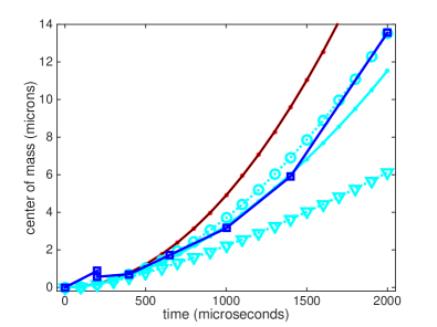
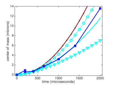
Figure 1: (Colour online) — Position of the center of mass as a function of time from the numerical simulations in comparison with the experimental data from Fig. 3 in Ref. Palzer2009, (blue open squares). The free-fall analytic solution $x(t)=gt^{2}/2$ is also shown for comparison (red solid dots). Top panel: numerical results at fixed density $n\simeq 1.2$ $\mu$m^-1, for $\gamma=1.9$ (cyan open circles), $\gamma=2.6$ (cyan solid dots), and $\gamma=4.0$ (cyan open triangles). Bottom panel: numerical results at fixed $\gamma=2.6$, for $n\simeq 0.84$ $\mu$m^-1 (cyan open circles), $n\simeq 1.2$ $\mu$m^-1(cyan solid dots), and $n\simeq 1.56$ $\mu$m^-1 (cyan open triangles).

In the simulations we consider an infinite 1D gas of uniform density. The experimental time $t=0$ in Ref. Palzer2009, was chosen to correspond to the middle of the RF pulse that creates the packet of falling atoms. Accordingly, we chose $t=0$ in our simulations as the time when the Fourier limited packet starts moving through the 1D gas.

The numerical results appear to be very sensitive to the values of $\gamma$ and $n$. This allows us to determine that the combination $n\simeq 1.2$ $\mu$m^-1 and $\gamma=2.6$ provides the best fit to the experimental data. (We note that particles begin to leave the 1D trapped gas after about $2$ ms, which corresponds to the longest time reported in Fig. 1. Such an effect may be responsible for the discrepancy that we observe between our numerics and the very last data point in the experiment.)

Our results are in contrast with earlier theoretical modelling Palzer2009 ; Rutherford2011 ; Knap2013 which achieved a similarly good fit to the experimental results by using the strongly interacting Tonks-Girardeau (TG) approximation Girardeau1960 corresponding to $\gamma=\infty$ within the 1D gas and then treating the interaction between the impurities and the 1D gas at mean field level with an intermediate interaction strength $\gamma=7$ (see also Appendix. B).

V Density Profile

In order to further test our approach, we computed the profile of the falling atoms at long times after they exit the 1D gas, which can be compared with the experimental results reported in Fig. 5 of Ref. Palzer2009, . Experimental results are available Palzer2009 for all three cases in Table 1. Unfortunately, a similar comparison was not carried out in earlier theoretical modelling Palzer2009 ; Rutherford2011 ; Knap2013 .

In our simulations, we approximate the 1D gas to have uniform density and fixed length, with parameters $N_{p}$ and $L$ as in the experiments. Once again, we find that the resulting density profile of the falling packet has a significant sensitivity on the value of $\gamma$, which allows us to readily identify which one gives the best fit.

The outcome is shown in Fig. 2.

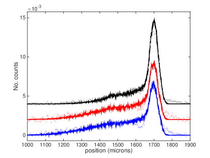
Figure 2: Behaviour starting from gaussian distributed initial conditions over $N_{\rm hist}=100,000$ histories, for $\gamma=1.1,1.9,2.1$ (black, red and blue, respectively) with a finite trap of uniform density (see text for size and density details). The results are expressed as histograms of the position of the particles after they have been falling for $18.6$ ms footnote: expm corrections long time . The corresponding experimental results in Fig. 5 of Ref. Palzer2009, are shown as thin dotted lines.

The experimental and simulation curves were normalised so that the area under the profiles equals $1$ (after subtraction of a background footnote: expm corrections background ). The main peak in the figure is due to the fraction of particles that fall freely through the 1D gas without scattering footnote: expm corrections long time .

Both the overall shape of the curves and the ratio between scattered and free-falling contributions are in reasonable agreement between numerics and experiments for $\gamma=1.1,\,1.9,\,{\rm and}\,2.1$, respectively. These results suggest that the relevant values of $\gamma$ in the experiments are those from the central region of the condensate.

We note that for these values of $\gamma$ we find very good agreement between the exact LL solution and the Bose gas (BG) approximation Bogoliubov1947 . In the BG limit, we studied also 1D gases with static position-dependent density footnote: 1D gas profile . We found that the resulting effects are minor and do not alter the best fit values of $\gamma$.

We notice that a small dip between the scattered peak and the free-falling peak appears in the experimental data (most noticeably at larger values of $\gamma$) whereas it is nearly absent in the numerical simulations. We conjecture that this dip might be due to the fact that in the actual experiment two or more impurities might fall though the trap at the same time. An effective attractive interaction between impurities could bind together nearby impurities and enhance the main peak at the expense of weight on either sides of the main peak. This effect is beyond our approximation and must be relegated to future research.

VI Conclusions

Using linear response theory and Fermi’s golden rule with exact transition rates to model the scattering between the driven impurity and the underlying 1D Bose gas, we have been able to obtain a quantitative description of the experimental results in Ref. Palzer2009, : center of mass, profile of driven packet with time-of-flight measurements and tomography. It appears that our crude approach is entirely sufficient to describe the vast majority of the observed physics. If desired, the approach taken here could be systematically improved by considering corrections of higher order in the coupling between the Bose gas and the impurity. The detection of finer quantum mechanical effects beyond our description may however require higher experimental accuracy.

In the range of $\gamma$ values considered here, the need for an exact LL solution was limited and the results would have been in large part the same had we used the BG approximation instead. However, sizeable differences between LL and BG arise already for $\gamma\gtrsim 3$, which is within experimental reach.

The case considered here can be viewed as an extremely simple example of handling a non-equilibrium situation in the presence of strong correlations. While the impurity is driven, the physics of the Bose gas can still be understood as remaining at equilibrium. Going further, one could try to understand how putting the gas itself out of equilibrium affects the impurity dynamics. Moreover, besides cold atom settings, one could also consider driven quantum magnets, for which the necessary exact correlators are also available. We will return to these issues in future work.

Appendix A Dependence on 1D gas density profile

For the values of $\gamma$ of relevance to the experiments in Ref. Palzer2009, , we find that our simulations give similar results whether we use the DSF from LL or in the BG approximation. We can therefore use the latter to test how the results are affected by (static) changes in the 1D gas density profile.

The DSF of a 1D bose gas can be determined directly from its spectrum Bogoliubov1947

$$\hbar\omega_{k} = \frac{\hbar^{2}k^{2}}{2m}\sqrt{1+\frac{4\gamma k_{F}^{2}}{\pi^{2}k^{2}}},$$ (6)

using the f-sum rule:

$$S(k,\omega) = \frac{N_{p}}{\hbar}\left[1+\frac{4\gamma}{\pi^{2}\left(k/k_{F}\right)^{2}}\right]^{-1/2}\!\!\!\!\!\!\delta(\omega-\omega_{k}).$$ (7)

After a few lines of algebra, following the steps outlined in Sec. II, one obtains that the only allowed outgoing wave vector is $k^{\prime}=\gamma k_{F}^{2}/(\pi^{2}k)$, with probability

$$\mathcal{P}_{k\to\gamma k_{F}^{2}/\pi^{2}k} = \left\{\begin{array}[]{lcl}\frac{2\gamma^{2}}{\pi^{3}}\frac{\varepsilon_{F}}{\hbar}\delta t\frac{k_{F}}{|k|}&&|k|/k_{F}>\sqrt{\gamma}/\pi\\ 0&&{\rm otherwise.}\end{array}\right.$$ (10)

Notice that Eq. (10) can be interpreted as a probability only if it is $\leq 1$, which in turn is satisfied if we choose

$$\delta t\leq\frac{\pi^{2}}{2\gamma^{3/2}}\frac{\hbar}{\varepsilon_{F}},$$ (11)

where we used explicitly the condition $|k|/k_{F}>\sqrt{\gamma}/\pi$.

Using Eq. (10) one can straightforwardly adapt the simulations to a position-dependent (static) density profile of the underlying 1D gas. For concreteness we fix the average density at the experimentally relevant value of $1.3278$ particles per micrometre (corresponding, in the case of uniform density, to an average $\gamma=1.9$). We then contrast the following cases: (i) a uniform condensate of finite length $L=24.1$ $\mu$m; (ii) a uniform condensate of the same length with a square depletion to half its density near its center (defined as $-2.0<x<2.0$ $\mu$m); (iii) a parabolic condensate of the same length and average density; and finally (iv) a parabolic condensate with a central depletion obtained by subtracting the Gaussian-smoothed Wigner function that we used to describe the initial distribution of the falling packet, Eq. (5), after setting $p=0$. The four different options are illustrated in Fig. 3.

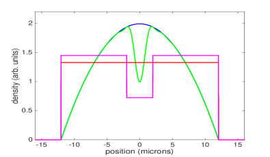
Figure 3: Different (static) density profiles for the 1D condensate used to assess how the shape affects the results of our simulations: (i) square (red), (ii) square with a square depletion at the center of the condensate (magenta), (iii) parabolic (blue), and (iv) parabolic with a Gaussian-smoothed Wigner function depletion at the center of the condensate (green).

The depleted cases are intended to mimic the effect of the decoupling laser that excites some of the atoms in the condensate to a non-trapped state, thus creating the initial packet of falling atoms (cf. Fig. 2 in Ref. Palzer2009, ). Note that we continue to neglect any feedback between the falling atoms and the condensate, nor we allow the latter to relax to a shape different form the initial one.

Fig. 4 shows the density profiles of the falling atoms at different times, using the same initial conditions discussed in the main text.

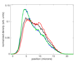
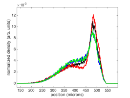
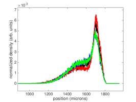
Figure 4: Density profiles at different times starting from the initial conditions discussed in the main text, averaged over $N_{\rm hist}=100,000$ histories. From left to right: $t=1.5$ ms, $t=10$ ms, and $t=18.7$ ms. The colours correspond to the four cases discussed in the text: (i) a finite uniform condensate (black); (ii) a finite uniform condensate with a square depletion at the center (red); (iii) a parabolic condensate (blue); and (iv) a parabolic condensate with a Gaussian-smoothed Wigner function depletion at the center (green).

The differences are minor and comparable to the experimental error bars in Ref. Palzer2009, . The case of a parabolic profile ought to be considered with care, since a continuously vanishing density at its edges implies large values of $\gamma$, and the BG approximation is no longer justified.

We notice that Ref. Johnson2011, , which considers a similar system in presence of a 1D optical lattice, also reported qualitatively similar results whether the 1D gas was prepared in equilibrium with or without the impurities (see the third paragraph in Sec.II D of Ref. Johnson2011, ).

Appendix B Tonks-Girardeau limit

In our work we have found quantitative agreement with the experimental results in Ref. Palzer2009, for small values of $\gamma$ where the BG approximation is reasonably accurate. This is in contrast with the modelling presented in that very same reference Palzer2009 , as well as the work done in Ref. Rutherford2011, and Ref. Knap2013, , which make use of the Tonks-Girardeau (TG) limit.

In this section we investigate the motion of the center of mass of the falling packet in the TG limit using our method. A reasonable agreement with the experimental results can be obtained only in the small $\gamma$ limit, which is in contradiction with the TG approximation. According to our simulations, already at intermediate values of the coupling strength (namely, $\gamma\gtrsim 7$) the falling atoms reach terminal velocity well within the time of the experiment, in contrast with the observed behaviour.

The dynamic structure factor of a 1D gas in the TG limit Girardeau1960 ($\gamma\to\infty$) can be written as

$$S(k,\omega) = \frac{N_{p}}{4\varepsilon_{F}}\frac{k_{F}}{k}\left[\Theta(\omega-\omega_{-})\Theta(\omega_{+}-\omega)\right.$$ (12)

$$\qquad\;\;\,-\left.\Theta(\omega-\omega_{+})\Theta(\omega_{-}-\omega)\right],$$

where

$$\omega_{\pm}(k)=\frac{\hbar{k_{F}}^{2}}{2m}\left|2\frac{k}{k_{F}}\pm\frac{k^{2}}{k_{F}^{2}}\right|.$$ (13)

Introducing the dimensionless wave vector notation $\tilde{k}=k/k_{F}$, after the usual substitution $k=k^{\prime}-k$ and $\omega=\hbar^{2}{k^{\prime}}^{2}/2m-\hbar^{2}k^{2}/2m$, a few lines of algebra show that the scattering probability density per unit of dimensionless wave vector, from $k$ to $k^{\prime}$, is given by

$$\mathcal{P}_{k\to k^{\prime}} = \begin{cases}\frac{\gamma^{2}}{\pi^{3}}\frac{\varepsilon_{F}}{\hbar}\delta t\frac{1}{|\tilde{k}^{\prime}-\tilde{k}|}&\textrm{if}\;\;|\tilde{k}|>1\;\;\textrm{and}\;\;|\tilde{k}^{\prime}|<1\\ 0&\textrm{otherwise.}\end{cases}$$ (14)

The expression above, which is correct to leading order in $\gamma$, presents the intrinsic problem that the total scattering probability at a given time,

$$\int^{+\infty}_{-\infty}\mathcal{P}_{k\to k^{\prime}}\>d\tilde{k}^{\prime}=\frac{\gamma^{2}}{\pi^{3}}\frac{\varepsilon_{F}}{\hbar}\delta t\left\lvert\ln\left(\frac{\tilde{k}-1}{\tilde{k}+1}\right)\right|,$$ (15)

diverges in the limit $k\to k_{F}$. For the stochastic approach to be valid, a necessary condition is that $\delta t$ be small enough so that the integrated probability at any given time remains smaller than $1$, which thus requires $\delta t$ to be vanishingly small for $k$ arbitrarily close to $k_{F}$.

The singularity is directly related to the limit $\gamma\to\infty$. However, it cannot be easily resolved by including the subleading correction in $1/\gamma$ because the expansion of $\mathcal{S}$ becomes negative in some range of $k$ and $\omega$ BrandCherny .

A compromise to obtain a non-negative, non-divergent probability is to use the expansion of $\mathcal{S}$ to leading order, as in Eq. (12), but to replace the Heaviside Theta functions with those from the Random Phase Approximation (RPA). Namely, we use the TG form of the DSF, but with support in $k$ and $\omega$ from RPA. This in turn means that the probability $\mathcal{P}_{k\to k^{\prime}}$ retains the same form as in Eq. (14), but it is set to zero identically outside the range:

$$\begin{cases}1-\frac{4}{\gamma}<\tilde{k}\leq 1&\frac{\gamma-4-\tilde{k}(\gamma-2)}{2}<\tilde{k}^{\prime}<1-\frac{2(1+\tilde{k})}{\gamma-2}\\ {\rm or}&\\ \tilde{k}>1&-\frac{\gamma-4+2\tilde{k}}{\gamma-2}<\tilde{k}^{\prime}<1-\frac{2(1+\tilde{k})}{\gamma-2},\end{cases}$$ (16)

and similarly for negative values of $\tilde{k}$. In the limit of $\gamma\to\infty$ this tends to Eq. (14), as one would expect. We tested our choice of probability regularisation in the TG limit by comparing its results with RPA and LL simulations for large values of $\gamma$ and we found good quantitative agreement (not shown).

Using the new boundaries in Eq. (16), the probability that a particle with wave vector $\tilde{k}$ scatters with the condensate in a time interval $\delta t$ (to any allowed $\tilde{k}^{\prime}$) remains finite for all allowed values of $\tilde{k}$. Namely,

$$\int_{[\gamma-4-\tilde{k}(\gamma-2)]/2}^{1-2(1+\tilde{k})/(\gamma-2)}\mathcal{P}_{k\to k^{\prime}}\>d\tilde{k}^{\prime} = \frac{\gamma^{2}}{\pi^{3}}\frac{\varepsilon_{F}}{\hbar}\delta t\ln\left[\frac{\gamma-2}{2}\right]$$

if $1-4/\gamma<\tilde{k}\leq 1$, and

$$\int_{-(\gamma-4+2\tilde{k})/(\gamma-2)}^{1-2(1+\tilde{k})/(\gamma-2)}\mathcal{P}_{k\to k^{\prime}}\>d\tilde{k}^{\prime} = \frac{\gamma^{2}}{\pi^{3}}\frac{\varepsilon_{F}}{\hbar}\delta t\ln\left[\frac{\tilde{k}+1-4/\gamma}{\tilde{k}-1+4/\gamma}\right],$$

if $\tilde{k}>1$. Notice that the maximum over $\tilde{k}>1$ of the logarithmic contribution in the second case is in fact the same as the first case: $\ln[(\gamma-2)/2]$. Our stochastic approach is therefore valid, provided that we choose

$$\delta t\lesssim\frac{\pi^{3}}{\gamma^{2}}\frac{\hbar}{\varepsilon_{F}}\left\{\ln\left[\frac{\gamma-2}{2}\right]\right\}^{-1}.$$ (17)

For the typical system parametres considered in this work, the upper bound for $\delta t$ scales as $(\gamma^{2}\ln\gamma)^{-1}$ milliseconds. This is satisfied for instance by choosing $\delta t\lesssim 0.01$ $\mu$s up to $\gamma=100$.

We can then implement our stochastic approach using the inverse transform sampling analytically in the TG limit. Fig. 5 shows the resulting behaviour of the centre of mass (CM) motion from TG simulations for a uniform 1D gas of density $n=1.2$ $\mu$m^-1 and $\gamma=4.1,\,5,\,6,\,8,\,10,\,25,\,100$, to be contrasted with the results presented in the main text, Fig. 1.

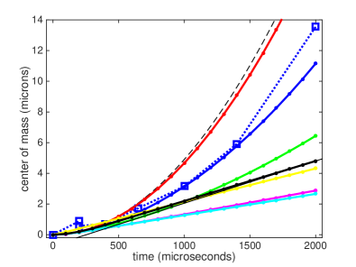
Figure 5: (Colour online) — Position of the center of mass as a function of time from our simulations in the TG limit, considering a uniform 1D gas with $n=1.2$ $\mu$m^-1 and $\gamma=4.1,\,5,\,6,\,8,\,10,\,25,\,100$ (red, blue, green, magenta, cyan, yellow, and black, respectively). The black dashed line represents the free-fall curve. The black solid line corresponds to the expected behaviour in the $\gamma\to\infty$ limit (i.e., terminal velocity $v_{F}$). Blue open squares (joined by a dotted line) represent the experimental data from Fig. 3 in Ref. Palzer2009, .

We notice that the CM motion becomes asymptotically linear in time within the simulation time window for $\gamma\gtrsim 7$, suggesting that the falling atoms reach terminal velocity. The value of the terminal velocity is non-monotonic in $\gamma$: it initially decreases (in agreement with Ref. Rutherford2011, ) with increasing $\gamma$, and later increases and tends asymptotically to $v_{F}$ in the $\gamma\to\infty$ limit, as expected.

Reasonable agreement with the experimental results can only be obtained in the weak coupling limit ($\gamma\sim 5$), which is in contradiction with the TG limit (and even with the RPA approximation, which has a hard limit of applicability of $\gamma>4$, and is known to begin to fit reasonably well the LL DSF only for $\gamma\gtrsim 10$ BrandCherny ).

References

- (1) S. Palzer, C. Zipkes, C. Sias, and M. Köhl, Phys. Rev. Lett. 103, 150601 (2009).
- (2) C. Zipkes, S. Palzer, C. Sias, and M. Köhl, Nature (London) 464, 388 (2010).
- (3) P. Wicke, S. Whitlock, and N. J. van Druten, arXiv:1010.4545v1 (2010).
- (4) J. Catani, G. Lamporesi, D. Naik, M. Gring, M. Inguscio, F. Minardi, A. Kantian, and T. Giamarchi, Phys. Rev. A 85, 023623 (2012).
- (5) T. Fukuhara, A. Kantian, M. Endres, M. Cheneau, P. Schauss, S. Hild, D. Bellem, U. Schollw ock, T. Giamarchi, C. Gross, I. Bloch, and S. Kuhr, Nat. Phys. 9, 235 (2013).
- (6) V. Hakim, Phys. Rev. E 55, 2835 (1997).
- (7) M. B. Zvonarev, V. V. Cheianov, and T. Giamarchi, Phys. Rev. Lett. 99, 240404 (2007).
- (8) G. E. Astrakharchik and L. P. Pitaevskii, Phys. Rev. A 70, 013608 (2004).
- (9) A. V. Ponomarev, J. Madroñero, A. R. Kolovsky, and A. Buchleitner, Phys. Rev. Lett. 96, 050404 (2006).
- (10) M. D. Girardeau and A. Minguzzi, Phys. Rev. A 79, 033610 (2009).
- (11) A. G. Sykes, M. J. Davis, and D. C. Roberts, Phys. Rev. Lett. 103, 085302 (2009).
- (12) A. Yu. Cherny, J.-S. Caux, and J. Brand, Phys. Rev. A 80, 043604 (2009).
- (13) D. M. Gangardt and A. Kamenev, Phys. Rev. Lett. 102, 070402 (2009).
- (14) T. H. Johnson, S. R. Clark, M. Bruderer, and D. Jaksch, Phys. Rev. A 84, 023617 (2011).
- (15) L. Rutherford, J. Goold, Th. Busch, and J. F. McCann, Phys. Rev. A 83, 055601 (2011).
- (16) J. Goold, T. Fogarty, N. Lo Gullo, M. Paternostro, and Th. Busch, Phys. Rev. A 84, 063632 (2011).
- (17) M. Schecter, A. Kamenev, D. M. Gangardt, and A. Lamacraft, Phys. Rev. Lett. 108, 207001 (2012).
- (18) J. Bonart and L. F. Cugliandolo, Europhys. Lett. 101, 16003 (2013); Phys. Rev. A 86, 023636 (2012).
- (19) C. J. M. Mathy, M. B. Zvonarev, and E. Demler, Nat. Phys. 8, 881 (2012).
- (20) M. Knap, C. J. M. Mathy, M. Ganahl, M. B. Zvonarev, and E. Demler, Phys. Rev. Lett. 112, 015302 (2012).
- (21) M. D. Girardeau, J. Math. Phys. 1, 516 (1960).
- (22) A. Yu. Cherny, J.-S. Caux, and J. Brand, Front. Phys. 7, 54 (2012).
- (23) In support of our choice of approach, we point out that Ref. Johnson2011, shows how a perturbative approach to study these systems appears to be valid beyond the perturbative regime. Moreover, both Ref. Ponomarev2006, and Ref. Johnson2011, demonstrate the appropriateness and effectiveness of a (semi-classical) stochastic description.
- (24) N. N. Bogoliubov, J. Phys. (USSR) 11, 23 (1947), reprinted in The Many-body Problem, edited by D. Pines (Benjamin, New York, 1961).
- (25) J.-S. Caux and P. Calabrese, Phys. Rev. A 74, 031605 (2006).
- (26) C. Sias and M. Köhl, (private communication).
- (27) For the relatively small values of that produce the best agreement with the experiments according to our simulations, we find that the exact DSF from LL calculations yields results similar to the DSF from the BG approximation. Within the BG approximation, we were then able to test the effects of a static non-uniform 1D gas density profile on our results and demonstrate that they are negligible (see Appendix A).
- (28) Smoothing of the Wigner function is required (over appropriately wide regions) to ensure non-negativity, as we want to interpret it as a probability distribution function (see Ref. Cartwright1976, ). The typical approaches are a sliding average over a constant interval, or a Gaussian convolution. We chose the latter for numerical tractability, as the result can be conveniently written in terms of error functions, Eq. (5).
- (29) N. D. Cartwright, Physica 83A, 210 (1976).
- (30) In the experimental data for and , we subtracted a background ( and , respectively, in optical intensity units) so that the right tail of the position distribution drops down to approximately zero. This is justified by the fact that such a background ought to be spurious, as it could only arise from atoms accelerating faster than m/s2 (unphysical).
- (31) We note that the time reported in Ref. Palzer2009, , ms, appears to be inconsistent with the position of the main peak. Assuming m/s2, the main peak of free falling atoms starting at in a gaussian packet centerd at should appear at m after ms. We find instead that a time of ms is in better agreement with the data and we used it in our simulations. This is consistent with the fact that the falling packet is created with a laser pulse of finite duration. Indeed, comparing the non-interacting data from Ref. Rutherford2011, with the analytical free-fall behaviour , we find that a shift s is needed to achieve good agreement, which is consistent with a difference between ms and ms.
- (32) J. Brand and A. Y. Cherny, Phys. Rev. A 72, 033619 (2005); A. Y. Cherny and J. Brand, Phys. Rev. A 73, 023612 (2006).