On the Mass–Metallicity–Star Formation Rate Relation for Galaxies at $z\sim 2$

Abstract

Recent studies have shown that the local mass–metallicity ($M_{*}$–$Z$) relation depends on the specific star formation rate (SSFR). Whether such a dependence exists at higher redshifts, and whether the resulting $M_{*}$–$Z$–SFR relation is redshift invariant, is debated. We re-examine these issues by applying the non-parametric techniques of Salim et al. (2014) to $\sim 130$ $z\sim 2.3$ galaxies with N2 and O3 measurements from KBSS (Steidel et al. 2014). We find that the KBSS $M_{*}$–$Z$ relation depends on SSFR at intermediate masses, where such dependence exists locally. KBSS and SDSS galaxies of the same mass and SSFR (“local analogs”) are similarly offset in the BPT diagram relative to the bulk of local star-forming galaxies, and thus we posit that metallicities can be compared self-consistently at different redshifts as long as the masses and SSFRs of the galaxies are similar. We find that the $M_{*}$–$Z$–SFR relation of $z\sim 2$ galaxies is consistent with the local one at $\log M_{*}<10$, but is offset up to $-0.25$ dex at higher masses, so it is altogether not redshift invariant. This high-mass offset could arise from a bias that high-redshift spectroscopic surveys have against high-metallicity galaxies, but additional evidence disfavors this possibility. We identify three causes for the reported discrepancy between N2 and O3N2 metallicities at $z\sim 2$: (1) a smaller offset that is also present for SDSS galaxies, which we remove with new N2 calibration, (2) a genuine offset due to differing ISM condition, which is also present in local analogs, (3) an additional offset due to unrecognized AGN contamination.

1. Introduction

The relationship between the stellar masses, gas-phase metallicities, and star formation rates of galaxies ($M_{*}$–$Z$–SFR) has received increasing attention over the past $\sim$5 years, both because of its conceptual simplicity and its potential to provide deep insight into the processes that regulate galactic star formation (SF) and drive galaxy evolution over cosmic time. While the local ($z\lesssim 0.3$) luminosity-metallicity and mass-metallicity ($M_{*}$–$Z$) relations have been studied for decades, beginning with Lequeux et al. (1979), only more recently has the star formation rate (SFR) been proposed as a second parameter in the local mass-metallicity relation (Ellison et al., 2008). The primary correlation shows metallicity increasing with stellar mass until a plateau is reached at log $M_{*}\sim$10.5 (Tremonti et al., 2004), while the general sense of the secondary dependence with SFR is that at fixed mass, galaxies with higher SFRs tend to be more metal poor (Ellison et al., 2008; Mannucci et al., 2010; Lara-López et al., 2010; Hunt et al., 2012).

Conflicting results on the characterization of the local $M_{*}$–$Z$–SFR relation have ignited debate over whether the reported secondary dependence on SFR could be spurious, and due to: sample selection effects (de los Reyes et al., 2015), correlated errors in the measurements of SFR and metallicity (Lilly et al., 2013), systematic errors in metallicities (Yates et al., 2012), or biases introduced by SDSS fiber spectroscopy (Sánchez et al., 2013). In de los Reyes et al. (2015), the limitations of previous parameterizations used to characterize the local relation and the need for non-parametric techniques to enable comparative analysis of different datasets were also highlighted.

Thus, to gain insight into the origins of the conflicting results, in Salim et al. (2014) we devised a non-parametric analysis framework based on the SFR offset from the local star-forming (“main”) sequence at a given $M_{*}$, and undertook a comprehensive re-analysis of the local $M_{*}$–$Z$–SFR relation using a Sloan Digital Sky Survey (SDSS) dataset together with GALEX ultraviolet and WISE infrared photometry. Studying the $M_{*}$–$Z$–SFR relation in terms of SFRs or specific SFRs (SSFRs) relative to typical values on the “main sequence” is more physically motivated than using absolute SFRs, which, to first order, scale with $M_{*}$ (Brinchmann et al., 2004). Although we concluded that the dependence on SSFR is not spurious (after investigating multiple SFR and metallicity indicators), the analysis exposed important features of the relationship. In particular, Salim et al. (2014) showed that adding the SFR as a second parameter does not greatly decrease the scatter in the $M_{*}$–$Z$ relation when the metallicities of individual galaxies, rather than the median-binned values are considered (i.e., the $M_{*}$–$Z$–SFR relation is not tight). We confirmed that the overall SFR dependence is weaker, or absent, at higher masses. However, at a given mass the dependence on SFR is much stronger for intensely star-forming galaxies above the “main sequence” (galaxies with high SSFR for their mass). We noted that simple parameterizations of the local $M_{*}$–$Z$–SFR relation (a plane, or the projection of least scatter in $Z$) do not capture this behavior of galaxies with high relative SSFR because the parametrizations are dominated by the bulk of “normal” galaxies along the core of the main sequence.

Recognizing the limitations of parameterizations of the local $M_{*}$–$Z$–SFR is particularly important in the context of testing its redshift invariance. The concept of invariant $M_{*}$–$Z$–SFR relation was put forward by Mannucci et al. (2010), who refer to a it as the “fundamental metallicity relation” (FMR). They showed that selected galaxy samples up to $z\sim 2.2$ lie along the projection of the local $M_{*}$–$Z$–SFR that minimizes the scatter in metallicity, i.e., that they are consistent with a non-evolving $M_{*}$–$Z$–SFR relation. $M_{*}$–$Z$ relations at $z>0$ then represent the slices of the invariant (i.e., fundamental) $M_{*}$–$Z$–SFR relation at (S)SFRs higher than those found in local galaxies. However, a number of more recent studies have concluded that $z\sim 2$ samples do not lie on the local $M_{*}$–$Z$–SFR relation, implying an evolving relation. Most of these studies were based on Mannucci et al. (2010) parametrization of the local relation (e.g., Cullen et al. 2014; Zahid et al. 2014b; Maier et al. 2014), except for Sanders et al. (2015), who performed a direct comparison with the local samples. The result of Sanders et al. (2015) highlights other possible causes for the discrepant results, e.g., an evolution in metallicity calibrations (e.g., Kewley et al. 2013; Steidel et al. 2014). Sample selection effects (Juneau et al., 2014), may also play a role. Establishing the existence of SFR dependence of $M_{*}$–$Z$ relation at higher redshifts would be important even if the resulting high-redshift $M_{*}$–$Z$–SFR relation did not coincide with the one followed by local galaxies. The evidence that SFR is a second parameter at $0.7<z<2.3$ is likewise inconclusive (Cresci et al., 2012; Zahid et al., 2014b; Wuyts et al., 2014; Steidel et al., 2014; Maier et al., 2014; de los Reyes et al., 2015; Sanders et al., 2015).

Armed with a more detailed, non-parametric characterization of the local $M_{*}$–$Z$–SFR relationship we can examine these points of contention in recent work involving galaxies at $z\sim 2$. Here, we will apply our analysis framework to re-examine whether a secondary dependence of the $M_{*}$–$Z$ relation on SFR also exists for higher redshift samples, and more generally, whether the local $M_{*}$–$Z$–SFR relation is invariant with redshift and describes star-forming galaxies at all stages of their evolution over cosmic time. We focus on the latest and most comprehensive $z\sim 2$ spectroscopic datasets (Steidel et al., 2014; Sanders et al., 2015). We present evidence that this approach is able to circumvent the thorny issues of inconsistent or evolving metallicity calibrations. We highlight the possible role of observational selection effects (Juneau et al., 2014) and/or the possibility that some high-mass high-redshift galaxies contain unrecognized contribution from AGN line emission.

2. Data and samples

Our analysis is primarily based on the dataset published in Steidel et al. (2014) from the Keck Baryonic Structure Survey (KBSS), a near-IR spectroscopic survey performed with the MOSFIRE multi-object slit spectrograph on the Keck I telescope. KBSS has obtained $H$ and $K$-band spectra of galaxies at $1.95<z<2.65$. The majority of targets had previously determined redshifts from optical spectroscopy and had been originally selected using a variety of techniques based on rest-frame UV colors (Adelberger et al., 2004; Steidel et al., 2004). The Steidel et al. (2014) analysis includes individual galaxies where the S/N ratios of [OIII]5007 and $\rm{H}\alpha$ line fluxes exceed 5, and those of [NII]6584 and $\rm{H}\beta$ exceed 2. For an average exposure time of 11000 s, these cuts corresponds to $\rm{H}\alpha$ and [OIII] $5\sigma$ limits of $\sim 10^{41.7}$ erg s^-1 (obtained from scaling MOSDEF sensitivity given by Coil et al. 2015). The published version of Steidel et al. (2014) presents 161 galaxies with both N2 = log[$F$([NII]6584)/$F(\rm{H}\alpha)$] and O3 = log[$F$([OIII]5007)/$F(\rm{H}\beta)]$ line ratios and an additional 31 galaxies with only the N2 measurements (i.e., currently lacking $H$-band observations). The total of 192 galaxies excludes seven objects identified as AGN based on broad emission lines or the presence of higher ionization species. Stellar masses were derived from SED fitting, and SFRs from $\rm{H}\alpha$ fluxes, corrected for slit losses and for extinction based on the continuum dust attenuation estimate from the SED fits. We note that the data used in our analysis, however, are the subset of the Steidel et al. (2014) sample, which was presented in the preprint version of their paper. We use the smaller, preprint sample because the published version of the paper omitted SFRs from the tables. Thus, the dataset used here contains 108 galaxies with both N2 and O3, and an additional 18 with N2, i.e., 2/3 of the published sample. Line ratios and stellar masses are taken from the published tables, and SFRs from the preprint. Differences between preprint and published line ratios are not significant (0.07 dex scatter, with no systematic offsets), so we assume that the SFRs have not changed significantly either, as also evidenced by a similar appearance of figures that involve SFRs in the preprint and the published paper.

We augment the analysis with measurements from the MOSFIRE Deep Evolution Field (MOSDEF) survey early observations (Kriek et al., 2014; Coil et al., 2015; Shapley et al., 2015). MOSDEF targets $H$-band selected galaxies at $2.1<z<2.6$ within the CANDELS survey areas. Targeting prioritization criteria include the availability of a spectroscopic redshift from previous work (40% of the sample), brightness, and photometric redshift in the target range. O3N2 ($=$ O3$-$N2) and N2-based metallicities were obtained for 53 galaxies for which all four lines have S/N ratio $>3$, corresponding to $\rm{H}\alpha$ and [OIII] $3\sigma$ limits of $\sim 10^{41.5}$ erg s^-1 (Coil et al., 2015). AGNs were removed from this sample based on X-ray and IR indicators, or if N2$>-0.3$ (Coil et al., 2015). Stellar masses come from SED fitting, and SFRs from $\rm{H}\alpha$ fluxes corrected for extinction using the Balmer decrement. Data tables with measurements for individual MOSDEF galaxies are not yet published. However, we used the published figures in Coil et al. (2015) and Sanders et al. (2015) to compare $M_{*}$–$Z$, SSFR–$M_{*}$ and O3–N2 relations from MOSDEF with those from SDSS and KBSS.

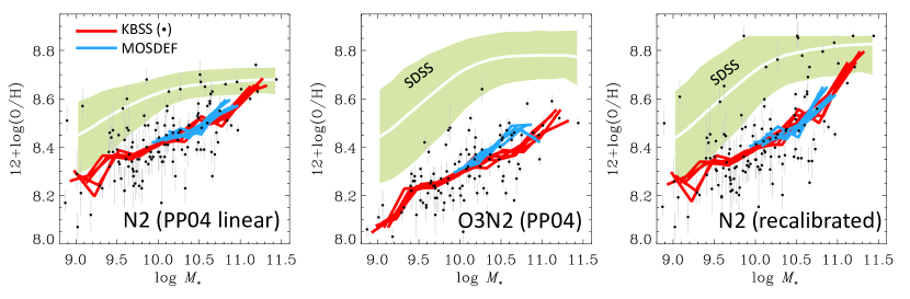
Figure 1.— The impact of the choice of metallicity indicator on inferred evolution in the $M_{*}$–$Z$ relation. Local ($z\sim 0$) sample comes from SDSS (green band is the 95 percentile range at a given mass; white line shows an average trend), while $z\sim 2$ data are from KBSS (black points; binned averages shown as red lines) and MOSDEF (binned averages shown as blue lines). MOSDEF averages are based on galaxies with $M_{*}\gtrsim 10$, for which their sample is not affected by incompleteness. Different average lines are obtained by varying the starting position for binning in fifths of the 0.25 dex bin width. Left (middle) panel is based on N2 (O3N2) line ratios, converted into metallicity using Pettini & Pagel (2004) linear calibrations. Right panel shows N2 after the recalibration is performed in order to bring N2 and O3N2 metallicities into a better mutual agreement for the SDSS sample. O3N2 shows a higher degree of “evolution” than N2, especially at higher masses. MOSDEF and KBSS MZRs agree between each other for N2, but depart to some extent for the more massive galaxies in the case of O3N2.

Comparison with the relations followed by local galaxies is based on the SDSS DR7 spectroscopic sample (Strauss et al., 2002; Abazajian et al., 2009) processed by the MPA/JHU group. Sample selection follows that of Mannucci et al. (2010), except that we extend the redshift range ($0.005<z<0.3$) as long as the mass included in the spectroscopic fiber is $>10\%$, following what we have done in Salim et al. (2014). Dropping the redshift limit from 0.07 to 0.005 removes low-SFR incompleteness for star-forming galaxies with $9<\log M_{*}<10$ (Salim et al., 2014). Typical mass-covering fraction of SDSS fiber spectroscopy is 30%, with 95 percentile range between 17% and 50%. Inclusion of lower-redshift galaxies, which have lower mass-covering fraction, does not affect any of the results. It is also important to note that the selection is based solely on S/N ratio in $\rm{H}\alpha$ being above 25. The limit on only the $\rm{H}\alpha$ line ensures that the sample is not biased in metallicity (Salim et al., 2014; Mannucci et al., 2010), while it is high enough that other required nebular lines will be well measured. Lowering the limit to values below 25 increases the number of galaxies with lower relative SSFR. However, these galaxies entirely follow the trends established by galaxies with higher S/N ratio, just with less precise metallicity measurements.

For initial analysis, we exclude SDSS galaxies that lie above the Kauffmann et al. (2003) AGN demarcation line. We use total (integrated) SFRs and stellar masses from the MPA/JHU catalog, which are determined following Brinchmann et al. (2004) and Salim et al. (2007), respectively, with additional details given in online documentation. Specifically, Brinchmann et al. (2004) SFRs are based on a hybrid combination of an emission-line based SFR within the spectral fiber and a photometric estimate outside of the fiber, and hence should capture the total activity of the galaxies.

A Chabrier IMF and standard cosmology ($H_{0}=70$ km s^-1 Mpc^-1, $\Omega_{m}=0.3$, $\Omega_{\Lambda}=0.7$) is assumed throughout the paper.

3. Method

As in Salim et al. (2014), we examine the metallicity as a function of the relative SSFR at fixed stellar mass. We define the relative SSFR as the offset from the local (SDSS) star-forming (“main”) sequence:

$$\Delta\log{\rm SSFR}=\log{\rm SSFR}-\langle\log{\rm SSFR}\rangle_{M_{*}},$$ (1)

where $\langle\log{\rm SSFR}\rangle_{M_{*}}$ is the median $\log{\rm SSFR}$ of galaxies with $M_{*}$. Alternatively (not used here), $\langle\log{\rm SSFR}\rangle_{M_{*}}$ can be a value obtained from fitting the local “main” sequence with some mean relation (e.g.,

$$\langle\log{\rm SSFR}\rangle_{M_{*}}=-0.35(\log M_{*}-10)-9.83$$ (2)

from Salim et al. 2007). We define relative SSFRs in reference to local main sequence (as opposed to high-redshift one) because the local SSFR–$M_{*}$ relation is more robustly known. In principle, relative SSFRs can be defined with respect to high-redshift sequence as well, and this change in zero point would not impact the analysis.

Using this simple analysis framework, one can determine if an SFR dependence is present without assuming a parametrization of the $M_{*}$–$Z$–SFR relation. Such non-parametric techniques are essential because they allow the dependence on the mass and SFR to be simultaneously explored, in contrast to a plane parameterization of Lara-López et al. (2010), which forces a fixed dependence on both the mass and the SFR, or the projection of least scatter in $Z$ of Mannucci et al. (2010), which forces a fixed SFR dependence at a given mass. Moreover, our methodology allows one to test whether high-redshift samples follow the same $M_{*}$–$Z$–SFR relation as the local galaxies without extrapolation of the assumed parametrization into regions which may not be well populated by local galaxies, and therefore do not carry much weight in the parameterization, but are occupied by high-redshift galaxies.

We will also apply a related non-parametric method for an even more direct test of $M_{*}$–$Z$–SFR invariance. The method consists in comparing the metallicities of $z\sim 2.3$ galaxies with the metallicities of their local “analogs”. A local “analog” is defined as an SDSS galaxy with $M_{*}$ and SSFR most similar to a given high-redshift galaxy, i.e., a galaxy for which the metric:

$$D^{2}=(\Delta\log{\rm SSFR})^{2}+(\Delta\log M_{*})^{2}$$ (3)

is minimized. Large volume of SDSS allows finding very close matches in SSFR and $M_{*}$ (small $D$). We use the word “analog” with caution, because we are not implying that such local galaxies undergo the same physical processes as the high-redshift galaxies, but only that in the context of invariant $M_{*}$–$Z$–SFR relation, the metallicities of high-redshift galaxies and the local “analogs” should be the same.

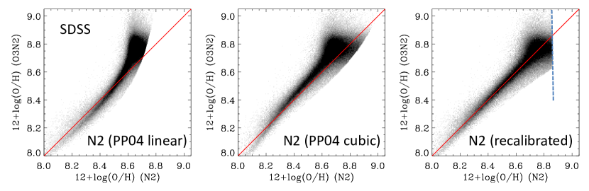
Figure 2.— Comparison of metallicities of SDSS galaxies derived based on O3N2 and N2 line ratios. O3N2 metallicity in all panels is derived from Pettini & Pagel (2004) calibration, while N2 metallicity is based on linear and cubic Pettini & Pagel (2004) relations (left and middle). One expects Pettini & Pagel (2004) calibrations, being local, to yield consistent metallicities for SDSS galaxies, but this is not entirely the case. We therefore recalibrate N2 calibration by assuming a rational functional form (Equation 5) and minimizing the deviations with respect to O3N2 metallicities. The resulting new N2 metallicities show no systematic offsets (right panel) and we use them for the remainder of the paper.

4. Main results

4.1. Mass–metallicity relations and the systematic differences in local metallicity calibrations

To set the stage for subsequent analysis, we start by inspecting the $M_{*}$–$Z$ plots (Figure 1), which compare the locus of SDSS galaxies with those from KBSS and MOSDEF samples. Left and middle panels of Figure 1 are based on N2 and O3N2 line ratios converted into metallicity using the calibrations of Pettini & Pagel (2004), which were derived using mostly direct-method abundances of HII regions in local galaxies. For N2, Pettini & Pagel (2004) provide linear and cubic calibrations. Figure 1, (left panel) uses linear calibration following KBSS and MOSDEF studies(Steidel et al., 2014; Sanders et al., 2015).

The first point to be emphasized from Figure 1 is that the $M_{*}$–$Z$ relations based on N2 and O3N2 metallicity indicators are not consistent even for SDSS galaxies, even though Pettini & Pagel (2004) calibrations have been based on local galaxies. Most notably, N2 metallicities at higher mass ($\log M_{*}\gtrsim 10$) are 0.11 dex lower than O3N2 metallicities. There are several reasons for the local mismatch, which can be best appreciated from Figure 2, where the metallicities of SDSS galaxies based on O3N2 and N2 indicators are compared directly. First, the linear N2 calibration is too crude to capture the saturation of N2 at high metallicities, and thus leads to a diverging offset (Figure 2, left). This point is relevant for 12+log(O/H)$>8.6$ and thus mostly affects the local samples which contain galaxies with such super-solar metallicities. The relationship between N2 and metallicity in this regime is somewhat better described with the cubic N2 calibration of Pettini & Pagel (2004), but there are still significant systematics at high metallicities (Figure 2, middle; also Kewley & Ellison 2008, their Figure 2). Second, Pettini & Pagel (2004) calibrator sample is relatively small (10²), so some differences due to the limited accuracy of the functional fitting are to be expected when the comparison is performed within a much larger (10⁵) SDSS sample. Furthermore, the Pettini & Pagel (2004) calibrator sample may not be entirely representative of a typical low-redshift population. Consequently, even for lower metallicities (12+log(O/H)$\sim 8.4$), the metallicity based on linear calibration of N2 is somewhat offset with respect to O3N2—it is $\sim 0.03$ dex higher (Figure 2, left). An offset of a similar magnitude, but in the opposite direction, is present for the cubic N2 calibration (Figure 2, middle). This discrepancy at lower metallicities will be important for high-redshift galaxies where measured metallicities tend to be lower. Thus, the 0.13 dex systematic difference between N2 and O3N2 metallicities of $z\sim 2.3$ samples (Newman et al., 2014; Zahid et al., 2014b; Steidel et al., 2014), which is usually attributed to evolution in one or both calibrations, is actually in part ($\sim 1/4$) due to the mismatch in local calibrations.

In order to be able to separate possible systematics arising from evolution (i.e., the inapplicability of local calibrations at high redshift) from those that stem merely from mismatch of the local metallicity scales, we recalibrate the N2 relation to match the metallicities resulting from Pettini & Pagel (2004) O3N2 calibration. We take O3N2 metallicities as fiducial because the O3N2 calibration is not subject to saturation, so it is more likely to be close to the linear form assumed in Pettini & Pagel (2004). The new N2 calibration is represented with a rational function that tends to a linear relation for low values of N2 (low metallicities), and has asymptotic behavior for high values. Its analytical form is:

$$12+\log({\rm O/H})_{\rm N2}=a+b\,{\rm N2}+c/({\rm N2}-d)$$ (4)

and ${\rm max}(12+\log({\rm O/H})_{\rm N2})=e$, where $a,b,c,d$ and $e$ are the free parameters obtained from the minimization of the sum of the binned median deviations of orthogonal offsets of points in Figure 2 from the diagonal (the 1:1 relation). Minimization is performed on binned values in order to give uniform weight at a range of metallicities. Parameter $d$ represents the position of the asymptote in N2, while $e$ is the value above which metallicities are assigned the value $e$. Parameter $e$ signifies the point above which N2 cannot provide reliable information on metallicity (except that it is high). The relation with the best-fitting parameters is:

$$12+\log({\rm O/H})_{\rm N2}=8.50+0.37{\rm N2}-0.15/({\rm N2}+0.10)$$ (5)

and ${\rm max}(12+\log({\rm O/H})_{\rm N2})=8.86$. For comparison, Pettini & Pagel (2004) linear calibration has parameters $a=8.90$, $b=0.57$, $c=d=0$. The comparison of new N2 metallicities with O3N2 is shown in Figure 2 (right). Systematic offsets are removed. In the remainder of the paper we will only use recalibrated N2 metallicities.

We return to the $M_{*}$–$Z$ relation, but now show the plot based on recalibrated N2 (Figure 1, right panel). SDSS loci of N2 and O3N2 metallicities now agree better. As expected, there is less change in trends of $z\sim 2$ samples, except that the total change in N2 metallicity from low-mass end to high-mass end is now greater, i.e., the $M_{*}$–$Z$ trend is steeper.

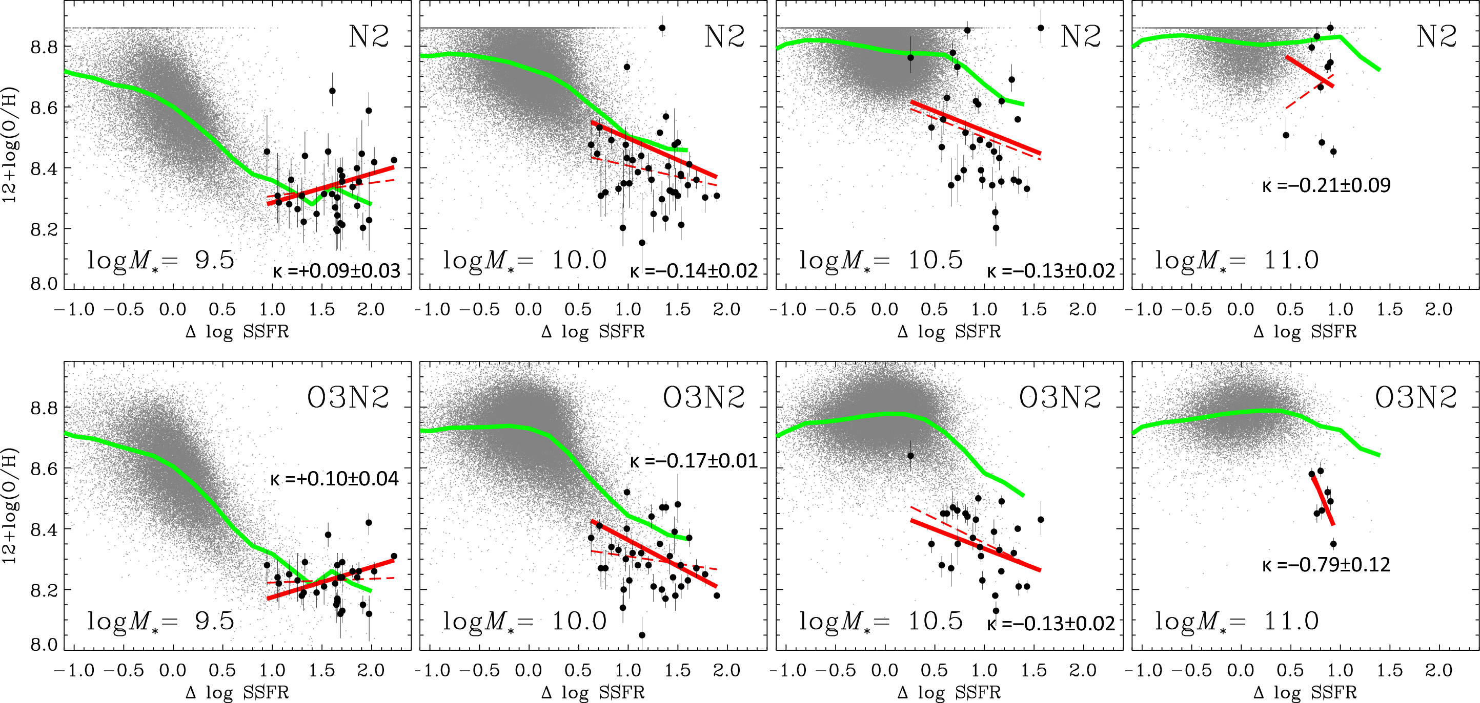
Figure 3.— Salim et al. (2014) non-parametric analysis technique for studying the $M_{*}$–$Z$–SFR relation. Metallicities of local and high-redshift galaxies are shown as a function of the relative SSFR (SSFR offset from the local star-forming sequence), in four 0.5 dex-wide mass bins. Metallicities are derived using two methods: O3N2 metallicities (lower panels) use Pettini & Pagel (2004) calibration, while N2 metallicities (upper panels) are based on our recalibration that forces agreement with O3N2 for local galaxies (Figure 2). Recalibration also caps N2 metallicities when N2 saturates. Black dots represent $z\sim 2.3$ galaxies from KBSS (Steidel et al., 2014), in comparison with SDSS galaxies (grey points). High-redshift data show a statistically significant anti-correlation at $\log M_{*}=10.0$ and 10.5 (panels B and C), as indicated by the red line (linear weighted fit). Formal slopes and their errors are indicated, but whether they are actually statistically significant given the sample size requires additional consideration (Section 4.2). Visually the correlations appear less robust because the points with larger metallicity errors contribute to the scatter. Dashed lines show unweighted linear fits. Green lines are binned averages for SDSS galaxies (0.2 dex wide bins). For both indicators, SDSS and KBSS trends agree in the lowest mass bin, but become offset in subsequent bins, with O3N2 offset being somewhat larger than N2 offset.

We now focus on high-redshift $M_{*}$–$Z$ trends in comparison with the local. The most striking difference is that the average N2 line ratios of the most massive galaxies ($\log M_{*}>11.0$) are similar for local and high redshift galaxies (albeit there is a large scatter), implying little metallicity evolution at the highest end, while the local and $z\sim 2$ $M_{*}$–$Z$ relations are quite offset in the case of O3N2, suggesting a strong evolution ($\sim 0.25$ dex). In Sections 4.4 and 5.3 we will discuss possible causes of this relative discrepancy.

Finally, from Figure 1, we also see that, regardless of the indicator, the metallicities of $z\sim 2$ galaxies do not saturate at high masses as they do locally, as pointed out in Steidel et al. (2014). KBSS and MOSDEF $M_{*}$–$Z$ relations generally agree for a given indicator, but with some differences in details, which will be discussed in Section 5.2. The average trends of KBSS and MOSDEF samples are based on galaxies that are individually detected in requisite lines (Section 2). For MOSDEF, we do not show the average $M_{*}$–$Z$ trends below $\log M_{*}\sim 10$, where many individual galaxies are not detected in [NII]6584 line (Kriek et al., 2014; Sanders et al., 2015). Otherwise, KBSS and MOSDEF $M_{*}$–$Z$ relations based on individual galaxies agree with the relations based on stacked spectra (Steidel et al., 2014; Sanders et al., 2015).

4.2. Specific SFR as a second parameter of $z\sim 2$ mass–metallicity relation

$M_{*}$–$Z$–SFR relation may be present at $z\sim 2$ even if it does not follow the local $M_{*}$–$Z$–SFR relation (i.e., is not redshift invariant), and we therefore first focus on establishing whether (S)SFR is a second parameter in KBSS sample. Figure 3 applies the analysis framework for investigating the $M_{*}$–$Z$–SFR relation, as introduced in Salim et al. (2014). N2 and O3N2 metallicities are examined against the relative SSFR in four 0.5 dex wide mass bins, for both the SDSS and KBSS samples. SSFRs for both sampels are relative to typical local values at that mass. O3N2 is based on Pettini & Pagel 2004 calibration, while N2 comes from our recalibration (Equation 5).

To test for SFR dependence we perform weighted and unweighted least square fits to KBSS points in each mass bin (full and dashed red lines in Figure 3). Weighted fits produce statistically significant non-zero slopes $\kappa$ ($Z$–SSFR correlations) in all mass bins for both metallicity indicators, except for $\log M_{*}=11.0$ bin for N2 ($\kappa=-0.21\pm 0.09$). The values of slopes are given in Figure 3. In general, the slopes of KBSS galaxies are comparable to those of SDSS galaxies at the same mass and SSFR. More specifically, like SDSS galaxies, KBSS sample shows an anti-correlation between $Z$ and SSFR in $\log M_{*}=10.0$ and 10.5 bins ($\kappa=-0.14\pm 0.02$ and $-0.13\pm 0.02$ for N2 and $-0.17\pm 0.01$ and $-0.13\pm 0.02$ for O3N2), for the two bins respectively.

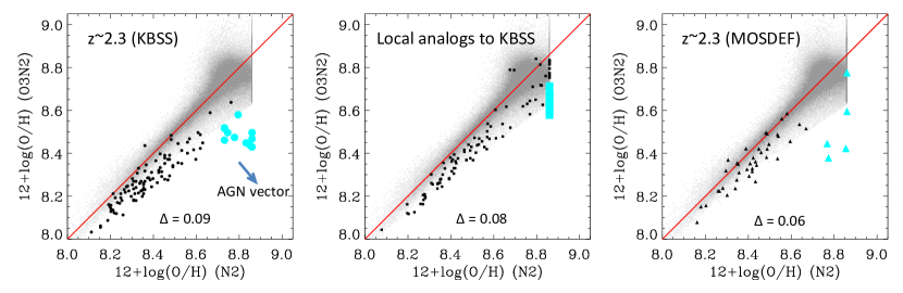
Figure 4.— Comparison of O3N2 and N2 metallicities of high-redshift samples (KBSS, left; MOSDEF, right) and local “analogs” to KBSS (middle). We define an analog to be a SDSS galaxy with the same SSFR and stellar mass as a KBSS galaxy. N2 metallicity is based on our recalibration which forces agreement with Pettini & Pagel (2004) O3N2 metallicities (Figure 2) for typical local galaxies (grey points). Local analogs to KBSS sample have a similar offset as KBSS and MOSDEF samples, validating the $M_{*}$–$Z$–SFR analysis approach that is based on relative comparison of metallicities of high-redshift and local galaxies of the same mass and SSFR. Possible AGN (N2$>-0.5$ and lying above the Kauffmann et al. 2003 line) are shown as cyan symbols and were excluded from calculating the average offset in N2 metallicity ($\Delta$), shown in each panel. The arrow in the left panel shows the direction and a possible magnitude of AGN contamination vector affecting the cyan points.

The formal slope errors do not take into account the uncertainties arising from small sample size. Therefore, to assess the statistical significance of anti-correlations we perform two additional tests: (a) we refit 100,000 bootstrapped samples and (b) we perturb the measurements by randomly drawing from a gaussian with $\sigma$ equal to the reported metallicity error and by 0.15 dex for SSFR, and refit the trends 100,000 times. In both tests we perform weighted fits. At $\log M_{*}=10.0$, the bootstrap test yields an anti-correlation in 94% of cases for N2 (99% for O3N2), while perturbed fits have a negative correlation in 99% of cases (100% for O3N2). Results are similar for $\log M_{*}=10.5$ bin: anti-correlation is present in 90% (96% for O3N2) of bootstraps and 91% (93% for O3N2) of perturbed fits. In the highest mass bin, the trend of KBSS galaxies is not statistically significant (there is a similar number of correlated and anti-correlated bootstraps). Currently the sample size in this bin is too small to establish if the metallicities of $z\sim 2$ galaxies, like the local galaxies of similar mass, lack the dependence on SSFR. In the lowest mass bin KBSS galaxies do not show an anti-correlation with SSFR, but neither do SDSS galaxies with such masses and SSFRs. While the overall SSFR dependence in SDSS at $\log M_{*}=9.5$ is quite strong, it appears to reach a low-metallicity plateau for SSFRs 1 dex or more above the main sequence. KBSS galaxies, which have such high SSFRs, also appear to have nearly contant metallicities.

We note that the visual impression of the significance of some of the correlations differs from the results of the formal analysis that, unlike by-eye estimate, takes metallicity errors into account. Indeed, the significance of slopes having a non-zero value when fitting is performed without weighting by metallicity error (dashed lines in Figure 3) is low, except for O3N2 galaxies in $\log M_{*}=10.5$ bin ($\kappa=-0.16\pm 0.06$). For the same reason (ignorance of weights), the visual impression of the vertical position of the best-fit linear trend does not always agree with the its position based on the weighted fit (e.g., $\log M_{*}=10.0$ bin for N2).

Overall, we conclude that SSFR does appear to be a second parameter in $z\sim 2$ $M_{*}$–$Z$ relation, at least in the range of masses where such dependence is clearly present in the local relation.

4.3. Redshift invariance of the mass–metallicity-SFR relation: standard assumptions

We now turn our focus to the question of the invariance of $M_{*}$–$Z$–SFR relation. In this section we will approach the analysis with standard assumptions regarding the local comparison sample and the interpretation of high-redshift line ratios. In subsequent sections we will investigate the effects of possible AGN contamination of high-redshift line ratios, and of high-redshift selection effects due to high [OIII] sensitivity threshold.

If the $M_{*}$–$Z$–SFR relation is redshift invariant, then at any given mass and SSFR, the average metallicities of SDSS galaxies should be statistically consistent with those from KBSS. Therefore, Figure 3 displays N2 and O3N2 line ratios as metallicities. However, significant discrepancies between N2 and O3N2 metallicities of high-redshift galaxies were found when local calibrations were used to derive them (Newman et al., 2014; Zahid et al., 2014b; Steidel et al., 2014; Sanders et al., 2015), suggesting “evolution” in one or both indicators. These offsets can be seen in Figure 4 for KBSS (left) and MOSDEF (right) samples. It may thus appear that possible “evolution” of metallicity calibrations would preclude the test of redshift invariance of an $M_{*}$–$Z$–SFR relation. However, Figure 4 (middle panel) shows that, remarkably, similar offset between N2 and O3N2-inferred metallicities is also present in local high-SSFR galaxies (we specifically show what we call the local “analogs” of the KBSS sample, see Section 3). We interpret this to mean that the critical limitation for the application of local calibrations at high redshift is not so much that they are local, but rather that they are based on typical local galaxies (or HII regions in such galaxies). Therefore, the relative comparison of line ratios of high-redshift galaxies and local galaxies of similar SSFR, which is at the essence of establishing the invariance of any potential $M_{*}$–$Z$–SFR relation, can be carried out regardless of the uncertainties involving the conversion of line ratios into absolute metallicities, i.e., without having to decide if it is N2 or O3N2 (or both) indicator for which the “local” calibration is off at high redshift (and for local galaxies with high relative SSFRs). With this important conclusion in hand, we proceed with the analysis.

Figure 3 compares metallicities of SDSS (grey dots with binned averages shown with green line) and KBSS galaxies (black points with linear fits shown by red line), using N2 (upper panels) and O3N2 (lower panels) metallicity indicators. We notice that SDSS galaxies extend into the range occupied by KBSS, i.e., in each bin there do exist local galaxies with SSFRs as high as those in $z\sim 2.3$ sample. While such galaxies are extremely rare today, they are present in the large volume probed by SDSS. Hence, direct comparison of local and $z\sim 2$ populations is possible, and parameterizations of the local $M_{*}$–$Z$–SFR relation do not need to be extrapolated into the range of SSFRs occupied by high-redshift galaxies in order to test for possible evolution.

Examination of Figure 3 shows that the average trends of both N2 and O3N2 line ratios for SDSS and KBSS generally agree at lower masses. However, an offset appears in $\log M_{*}=10.0$ bin, in the sense that KBSS metallicities are lower, especially for O3N2. At $\log M_{*}=10.5$ the offset grows to $\sim 0.25$ in O3N2, but is somewhat smaller for N2, where it is compensated by scatter towards higher metallicities. The offset stays large for O3N2 at $\log M_{*}=11.0$, but is again somewhat smaller for N2. Interestingly, even in bins in which the offsets between average trends are large, there typically do exist SDSS galaxies with such low metallicities as KBSS galaxies.

The exact degree of offsets between the SDSS and KBSS trends depends on how one chooses to treat the data. If metallicity weights are ignored, as in fitting by-eye, the trend for, e.g., N2 in $\log M_{*}=10.0$ bin becomes more offset from the SDSS (dashed line). Thus we also perform an additional, more direct test of invariance. Instead of comparing the trends in various mass bins, we now study the difference in metallicity between KBSS galaxies and their local “analogs” from SDSS (i.e., the galaxy with matching SSFR and $M_{*}$, see Section 3, and lying below the Kauffmann et al. 2003 AGN demarcation line). We show the differences in metallicities for each KBSS–analog pair against its stellar mass (Figure 5). Redshift-invariant relation requires a lack of systematic offsets. We see that this is the case below $\log M_{*}\sim 9.7$, but above it the systematic difference appears, confirming the results from $Z$–SSFR analysis. In a 0.5 dex interval centered at $\log M_{*}=10.5$ the average difference is $-0.23\pm 0.04$ dex for N2 and $-0.28\pm 0.03$ dex for O3N2 (errors of offsets were obtained from bootstrapping resampling; they are not standard deviations).

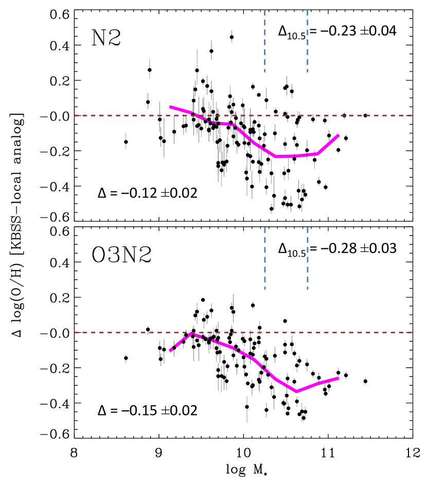
Figure 5.— Metallicity difference of KBSS galaxies and their local “analogs” in SDSS using N2 (upper panel) and O3N2 (lower panel) indicators. Analog is a galaxy with matching SSFR and stellar mass. The offset is mass dependent. The vertical error bar includes only the uncertainty of KBSS metallicity, as listed in Steidel et al. (2014), so it is a lower limit of the full uncertainty of the metallicity difference. Colored line show binned averages. Dashed lines show the interval centered on $\log M_{*}=10.5$ used to calculate the average offset at high mass ($\Delta_{10.5}$).

Figure 6.— Metallicity difference of KBSS galaxies and their local “analogs” in SDSS. Same as Figure 5, except that we now apply a correction to galaxies whose line measurements may be affected by an AGN contribution (cyan dots in Figure 4, left). The overall effect of the correction is relatively subtle, but it does produce more consistent offsets for N2 and O3N2 indicators, for the entire sample ($\Delta$), and at higher mass ($\Delta_{10.5}$).

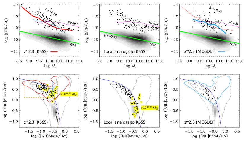
Figure 7.— Comparison of $z\sim 2.3$ KBSS (left), their local SDSS analogs (middle) and $z\sim 2.3$ MOSDEF samples (right), in terms of SSFR–$M_{*}$ plane (upper row), and the BPT diagrams (lower row). Green lines in the upper row represent a linear fit to the SDSS SF sequence (Equation 2, greyscale). High-redshift samples, especially KBSS, have steep slopes of SSFR vs. mass compared to local galaxies, or even compared to other surveys at that redshift (3D-HST, Whitaker et al. 2014). High-redshift surveys cannot detect emission lines of potential galaxies in the lower part of the BPT diagram (red and blue contours show SDSS galaxies with [OIII] and $\rm{H}\alpha$ luminosities above KBSS and MOSDEF detection limits). The lower part of the BPT diagram is where locally the more massive galaxies are found (yellow dots in left and middle lower panel have $\log M_{*}>10.25$). Dashed vertical line in lower left panel shows separates on the right possible AGN in KBSS. Rectangle in the lower left panel displays the selection of SDSS galaxies that mimics the region detected and occupied by KBSS sample, which admits some galaxies that lie above the local AGN demarcation line (blue curve, Kauffmann et al. 2003).

4.4. Redshift invariance: AGN contamination

From the analysis presented so far we would conclude that the $M_{*}$–$Z$–SFR relation is altogether not invariant, because of the systematic differences in metallicities at larger masses. The differences tend to be larger using the O3N2 than N2 indicator. This discrepancy could be the result of unrecognized AGN contribution to emission lines. Namely, AGN contribution moves a galaxy along the AGN mixing sequence in the BPT diagram Baldwin et al. (1981) (i.e., O3 vs. N2 diagram), increasing both N2 and O3. The increase in O3 is larger than in N2, so net O3N2 ratio increases as well. Larger N2 gives higher apparent metallicity, while larger O3N2 gives lower apparent metallicity, giving rise to a discrepancy.

In Figure 7 (lower left) we show the BPT diagram for KBSS sample. Some galaxies, especially with larger N2 values (N2$>-0.5$) are found away from the locus of the rest of the galaxies, along what may be an AGN spur. These galaxies tend to be more massive. These possible AGN-contaminated galaxies are shown as cyan dots in Figure 4 (left), in which we directly compared derived O3N2 and N2 metallicities. These candidate AGN indeed lie even further from the 1:1 diagonal than the rest of the KBSS sample. Similar effect was reported in Newman et al. (2014). Moving a galaxy up the AGN mixing sequence increases O3 and N2 such that $\Delta{\rm O3}\approx 5\Delta{\rm N2}$. For $\Delta$O3 = 0.4 dex, which appears as a reasonable value from inspecting Figure 7, the resulting O3N2 “metallicity” decreases by 0.10 dex, while the N2 “metallicity” increases by 0.12 dex, i.e., galaxy is shifted almost perpendicular to the diagonal in Figure 4 (arrow in the left panel). Similar shift is seen in several MOSDEF galaxies (right panel).

Is it realistic to have unrecognized AGNs in the KBSS (and MOSDEF) samples? KBSS excluded high ionization species emission-line galaxies as being contaminated by AGN. This method is only sensitive to more energetic AGNs (ionization potentials for C IV and N V are 48 and 77 eV, respectively, compared to 15 eV and 35 eV for [NII] and [OIII]). A similar method applied to the SDSS would not identify as AGN many of the galaxies on the AGN branch of the BPT diagram. Line ratio diagnostics may be the only practical method to recognize weaker AGN even locally.

How does the possible AGN contamination bear on testing the $M_{*}$–$Z$–SFR redshift invariance? In Figure 6 we again show the difference between the metallicities of KBSS galaxies and their local analogs as a function of mass, but we now correct the metallicities of AGN candidates by $-0.10$ dex for N2 metallicity (13 galaxies) and $+0.12$ dex for O3N2 metallicity (11 galaxies). Systematic offsets remain, especially at high masses, but they are now nearly identical for N2 and O3N2 metallicities ($-0.13$ dex overall and $-0.26$ dex at $\log M_{*}=10.5$).

4.5. Redshift invariance: [OIII] sensitivity threshold

In this section we explore whether the sensitivity of high-redshift spectroscopic surveys (Juneau et al., 2014) affects the analysis of the evolution of the $M_{*}$–$Z$–SFR relation.

To illustrate the potential issue with sensitivity, we again examine the BPT diagrams in Figure 7 (KBSS, lower left panel; MOSDEF, lower right panel). Both $z\sim 2.3$ samples are confined to the upper part of the diagram, which is locally dominated by lower metallicity galaxies. What is interesting is that the regions of the BPT diagram to which the current high-redshift spectroscopic surveys are sensitive to (shown with red and blue contours in KBSS and MOSDEF BPT diagrams, respectively), largely coincide with the locus of individual detections. (The sensitivity contours were obtained by selecting SDSS galaxies having [OIII]5007 and $\rm{H}\alpha$ luminosities above KBSS/MOSDEF survey limits (Section 2), following Juneau et al. 2014.) If galaxies at $z\sim 2$ existed in the lower portion of the BPT diagram, current surveys would not include them in their samples, because they require [OIII]5007 line detection.

We can also use local “analogs” to illustrate the nature of this potential issue. Like KBSS and MOSDEF, the local “analogs” to KBSS galaxies are offset upwards in the BPT diagram (Figure 7 , lower middle panel), but unlike the $z\sim 2$ samples, the local “analogs” to the KBSS sample populate the full extent of the star-forming branch in the BPT diagram, with the majority of the more massive “analogs” having low O3 (yellow points indicate $\log M_{*}>10.25$). The difference in the extent of the locus of the “analogs” on the BPT diagram with respect to $z\sim 2$ samples is essentially another way of saying that the $M_{*}$–$Z$–SFR relation shows no offset at lower masses (upper part of the BPT diagram), but becomes increasingly discrepant at higher masses, because the locally higher-mass galaxies populate the lower regions of the BPT diagram, while they are (intrinsically, or perhaps because of sensitivity limits) found only in the upper parts at high redshift.

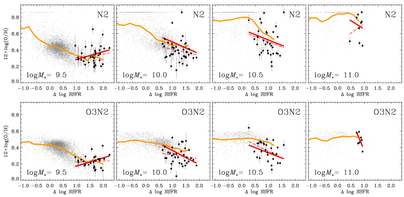
Figure 8.— Dependence of N2 and O3N2 metallicity on the offset from the local star-forming sequence for $z\sim 2.3$ galaxies (black dots) and SDSS galaxies (grey points) selected from a similar region of the BPT diagram as occupied by high-redshift samples (rectangle in Figure 7, lower left). Selection is modified from the standard one in order to allow for the possibility that high-redshift surveys miss galaxies in regions of the BPT diagram that they are not sensitive to, and to allow for the possibility of AGN contamination. The agreement between line ratio (metallicity) trends is improved, i.e., in this scenario the redshift invariant $M_{*}$–$Z$–SFR relation would be viable. However, other evidence disfavors the existence of a $z\sim 2$ high-metallicity population. See also Figure 3 caption, except that binned averages for SDSS are now shown as orange lines.

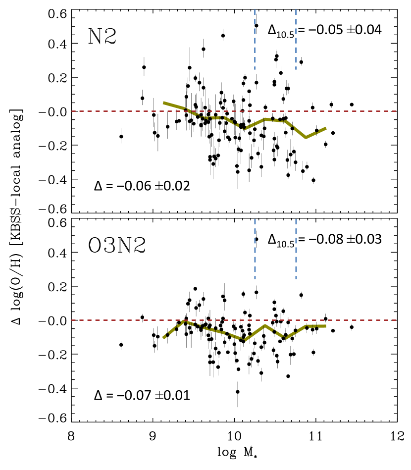
Figure 9.— Metallicity difference of KBSS galaxies and their local “analogs” in SDSS. Analogs are now selected from among the SDSS galaxies that occupy a similar region of the BPT as high-redshift samples, in order to account for the possibility that high-redshift surveys miss galaxies in regions of the BPT diagram that they are not sensitive to, and to allow for AGN contamination. The offsets are reduced compared to standard selection/assumptions (Figure 5), but are not entirely eliminated.

To understand the possible consequences of the insensitivity of high-redshift surveys to galaxies with low O3 ratios (high metallicities), we repeat the analysis, but now select SDSS galaxies only from the region of the BPT diagram accessible to, and occupied by KBSS galaxies ($0.1<{\mathrm{O}3}\leqslant 0.9$, and $-1.7<{\mathrm{N}2}<-0.3$, shown with the rectangle in Figure 7, lower left). This selection box will also admit some SDSS galaxies that are found above the AGN demarcation line, therefore implicitly “correcting” for the possibility that $z\sim 2$ samples are also affected by AGN contribution. We therefore do not apply any explicit AGN correction as we did in Section 4.4.

The new set of $Z$-SSFR plots is presented in Figure 8. The offset between SDSS and KBSS trends has generally reduced compared to Figure 3. The large offset in the $\log M_{*}=11$ bin is eliminated, and is greatly reduced in the $\log M_{*}=10.0$ and 10.5 bins. The improved agreement arises primarily because the local galaxies with high metallicity, which the $z\sim 2$ surveys would not be sensitive to, are now excluded from the comparison. These galaxies pushed the average metallicity trend of SDSS galaxies upwards.

We also repeat the analysis in which we directly compare the metallicities of KBSS galaxies with their local “analogs”, except that we select the analogs from the rectangle in Figure 7, lower left. The average trends of metallicity difference in Figure 9 confirm that the discrepancies at higher masses are significantly reduced, although they are not completely eliminated. At $\log M_{*}\sim 10.5$ the offset is now $-0.05\pm 0.04$ for N2 and $-0.08\pm 0.03$ for O3N2. N2 and O3N2 offsets are comparable. The overall offset (at all masses) is now $-0.06\pm 0.02$ with N2, and nearly identical with O3N2.

The above analysis demonstrates that our ability to constrain the metallicity evolution at higher masses hinges on an implicit assumption used in all studies so far that there do not exist significant populations of high-redshift galaxies in regions of the BPT diagram that are not accessible to observations (low O3 values). May such high-redshift populations exist? The fact that the ISM conditions at $z\sim 2$ appear to be somewhat more extreme than they are in typical local galaxies (Coil et al., 2015) does not preclude populating the lower (high-metallicity) portion of the BPT diagram. This is evident from the position of local analogs in Figure 7 (middle lower panel), which follow the “more extreme” location of KBSS galaxies in the upper part of the BPT diagram, but nevertheless also populate the lower portions. It is obviously important to understand if observational threshold actually produce any such biases. Because we do not have access to original KBSS and MOSDEF data, we base this discussion on the inferences from published results.

Shapley et al. (2015) tested whether non-detections create a bias in the BPT distribution for the MOSDEF sample. They produced average-stacked spectra, in mass bins, that included both the detections and the non-detections. The stacked spectra had line ratios that placed them in the region of BPT values shared by the detections (O3$>0.2$, their Fig. 2, left). Because the line ratios are distributed log-normally, median stacking of spectra would be preferred to average stacking, however, the results of such exercise produce similar results (A. Shapley, priv. comm.) A more stringent test would involve stacking only the non-detections. However, even the stacked spectra of non-detections are unlikely to fall in the lower part of the BPT diagram because the majority of non-detections in both KBSS and MOSDEF are galaxies with weak [NII], and not with weak [OIII]. Furthermore, the detection fraction tends to be high ($>80$%) at higher masses. Therefore, it appears that high-redshift samples, modulo some other sample selection bias (Section 5.1), are not biased by high [OIII] detection thresholds, i.e., they are probably not missing a significant population of high-metallicity galaxies. Consequently, the fact that the position of $z\sim 2$ samples in the BPT diagram matches the regions that these surveys are sensitive to (Figure 7) appears to be a mere coincidence, and a gap between local and high-redshift $M_{*}$–$Z$–SFR relations cannot be attributed to sensitivity issues. Nevertheless, we suggest that future studies should consider this issue.

5. Open questions

5.1. Are KBSS and MOSDEF spectroscopic samples representative of star-forming galaxies at $z\sim 2$?

In order to robustly assess the evolution of chemical enrichment from $z\sim 2$ to the present day, one requires both the high-redshift and the local samples to represent typical star-forming galaxies at that redshift. It is currently uncertain whether this is the case for high-redshift spectroscopic samples. The distribution of KBSS and MOSDEF data in SSFR–$M_{*}$ plane is different from what is expected. The slope of the star-forming sequence of KBSS sample is very steep ($\beta=-0.84$), significantly steeper than $\beta=-0.35$ slope of the local galaxies (Equation 2; green line in the upper panels of Figure 8). This disagrees with most results that suggest that the slope at $z\sim 2$ is similar or shallower than the local slope (Speagle et al., 2014). Recently, Whitaker et al. (2014) have determined the star-forming sequence at $z\sim 2.3$ based on an extensive dataset from 3D-HST survey (purple line in Figure 7 upper panels). As expected, the slope of the 3D-HST main sequence is somewhat shallower than the local one (we get $\beta=-0.19$), in sharp contrast to KBSS. At $\log M_{*}<9.7$ the 3D-HST sequence is lower than the KBSS sequence (but not MOSDEF), probably due to the KBSS’s UV selection, as mentioned in Steidel et al. (2014). However, the situation reverses at $\log M_{*}>9.7$, where both KBSS and MOSDEF have lower SSFRs than 3D-HST, up to 0.4 dex at $\log M_{*}\approx 11$. This high-mass offset has not been discussed in the literature so far. Altogether, it appears that the $z\sim 2$ spectroscopic samples target somewhat more intense star-formers at lower mass and more quiescent galaxies at higher mass. This potential bias does not directly affect for our $M_{*}$–$Z$–SFR relation analysis because we are comparing SDSS and KBSS galaxies at the same specific SFR. Nevertheless, it is important to fully understand if spectroscopic samples are representative of underlying star-forming population at $z\sim 2$, especially at high mass, where we find that the $M_{*}$–$Z$–SFR relations have an offset.

5.2. Are there systematic differences between KBSS and MOSDEF line ratios?

The $M_{*}$–$Z$ relations produced using KBSS and MOSDEF data on individual detections agree very well (Figure 1), except above $\log M_{*}=10.2$ for O3N2, where MOSDEF metallicities start to diverge from KBSS ones, the latter being lower.

The discrepancy between MOSDEF and KBSS measurements has been discussed in Shapley et al. (2015) in terms of the position of the galaxies in the upper portion of the star-forming branch in the BPT diagram. Here we perform similar analysis, but quantify the differences between the samples by finding the value O3_med, such that the curve:

$${\rm O3}=\frac{0.61}{{\rm N2}+0.08}+{\rm O3_{med}}$$ (6)

divides the sample in half. This function has only one free parameter: O3_med. The values of the other two parameters are fixed to the values used by Kewley et al. (2013) to describe the star-forming locus at $z=0$. Steidel et al. (2014) have allowed all three parameters to be free, but we find that the single-parameter form with other parameters fixed to local values actually better describes the high-redshift samples after possible AGN-contaminated galaxies are taken out. Furthermore, a single-parameter expression, i.e., a shift in the O3 direction, makes it easier to compare different samples. For local galaxies Kewley et al. (2013) find O3_med=1.1. For high redshift samples and their local analogs we focus only on the upper left part of the BPT diagram (N2$<-0.5$, O3$>0.0$), thus excluding possible AGN contamination (see also Figure 4) and outliers. For KBSS we obtain O3_med=1.32, i.e., its star-forming branch lies some 0.2 dex higher in the BPT diagram than the local one. For MOSDEF, we get O3_med=1.20, which, while higher than the local value, is significantly lower than the KBSS value. Local analogs to KBSS yield O3_med=1.28, which is closer to KBSS than MOSDEF, and also much higher than the typical local galaxies. That the local galaxies with high relative SSFRs were offset in the BPT diagram was previously found in Brinchmann et al. (2008).

Shapley et al. (2015) ascribe the difference between the position of KBSS and MOSDEF samples in the BPT diagram sample selection: UV selection of KBSS sample as opposed to the optical selection of MOSDEF. However, it is not clear whether selection is the main culprit. Inspecting the SSFR–$M_{*}$ distributions of the two samples (Figure 7 upper left and right), they appear similar, except at $\log M_{*}<9.5$ where KBSS sample has higher SSFRs and extends to lower masses. Even when we restrict the KBSS sample to mass range that both KBSS and MOSDEF appear to cover in similar fashion ($9.5<\log M_{*}<10.5$), we still obtain O3_med=1.29, a significantly higher value than for MOSDEF . Local analogs in the same mass range yield O3_med=1.27, i.e., very close to KBSS value. Future studies should be able to pin down the source of the discrepancy. The analysis presented here suggests that the cause may not be solely the differences in sample selection.

We also wish to point out that while O3_med are similar for KBSS and their local analogs, the former have a larger scatter (presumably because of larger measurement errors), which is why they more often cross the local AGN demarcation line than their analogs, which are found close to the line but do not cross it. Indeed, if we increase O3 values of analogs by the difference in O3_med between the analogs and KBSS (0.046 dex), only 6 out of 71 galaxies from the upper left of the BPT diagram would actually cross the Kauffmann et al. (2003) line. This suggests that $z\sim 2$ galaxies without AGN contribution intrinsically mostly lie below the Kauffmann et al. (2003) line. This conclusion would be even stronger for MOSDEF, whose O3_med is lower than that of KBSS analogs. We conclude that had the $z\sim 2$ line ratios had the same precision as in SDSS, the Kauffmann et al. (2003) AGN classification line would not require a shift greater than 0.05 dex in the vertical direction. The appearances are significantly different because of the larger measurement error that contributes to the scatter and because some of the galaxies that are currently not considered to be AGN probably are AGN. Allowing for larger observational errors, but still removing the potential AGN may be achieved using a simple cut in O3 and N2:

$${\rm N2}>-0.5{\rm and}{\rm O3}>0.1,$$ (7)

which resonates with the conclusions of Coil et al. (2015) that were based on the MOSDEF sample.

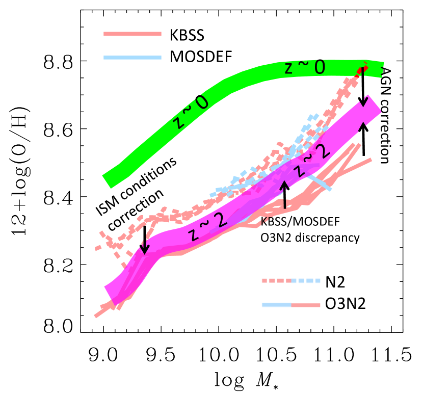
Figure 10.— Evolution of the mass-metallicity relation from $z\sim 2$ to today. Concordant high-redshift $M_{*}$–$Z$ trend (violet band) is a qualitative illustration of how to reconcile the $M_{*}$–$Z$ relations based on O3N2 (solid lines) and N2 (dashed lines) metallicity indicators, from KBSS (red) and MOSDEF (blue) surveys. To do so we consider various systematics discussed in Section 5.3 and labeled in the figure. Generally, at lower masses the concordant trend is closer to O3N2 because N2 will be more affected by the change in the N/O ratio, and at higher masses it is between N2 and O3N2 trends because of the possible AGN contamination that boosts N2 but suppresses O3N2.

5.3. Towards the concordant evolution of mass-metallicity relation

In this section we will attempt to arrive at a consistent $M_{*}$–$Z$ relation at $z\sim 2$ and discuss its evolution. This requires the knowledge of absolute metallicities. As discussed in Section 4.3, the analysis of $M_{*}$–$Z$–SFR invariance, being relative, could be carried out even without the knowledge of absolute calibrations that would be needed to convert the line ratios of high-redshift galaxies (and their local analogs) into metallicities. This is not the case if we are interested in constructing the $M_{*}$–$Z$ relations. The remaining offset between N2 and O3N2 “metallicities” even after we have corrected for a mismatch that was present in Pettini & Pagel (2004) relations, and have corrected for possible AGN contribution (Figure 4), means that either or both of the local calibrations does not hold for ISM conditions in $z\sim 2$ galaxies and their local analogs.

Whether N2 or O3N2 is more affected by the changes in the ISM conditions is currently a matter of debate. Masters et al. (2014) and Shapley et al. (2015) argue for O3N2 being less affected because $z\sim 2$ galaxies appear to follow local galaxies in O3 vs. S2 (= log([SII]6573/$\rm{H}\alpha$)) and O32 vs. R23 diagrams. Such diagnostics may not be particularly relevant in the context of O3N2 vs. N2 debate because using O3, and especially O32, results in comparing high-redshift galaxies with local galaxies having high ionization parameters, which, as we have shown, also exhibit the O3N2 vs. N2 discrepancy. Steidel et al. (2014) consider O3N2 to be less biased than N2 based on a very small number of direct metallicities of the local “green pea” galaxies, while Liu et al. (2008) reach a similar conclusion based on direct metallicities of stacked SDSS galaxies with high O3 values. On the other hand, Zahid et al. (2014b) consider N2 to be more reliable based on the greater sensitivity of O3N2 to changes in the ionization parameter, which many studies (Brinchmann et al., 2008; Nakajima & Ouchi, 2014; Kewley et al., 2013) assume to be the principal difference between ISM conditions of local and high-redshift galaxies. In contrast, Steidel et al. 2014 show, using photoionization models, that the ionization parameter cannot be the only factor driving the difference. The greater effect of the ionization parameter on O3N2 may be countered by higher N/O ratio at $z\sim 2$ compared to typical local galaxies of the same metallicity, as tentatively measured by Masters et al. (2014), thus making O3N2 more reliable for high-redshift studies than N2 in the end.

For the purposes of the remaining discussion we will assume that O3N2 provides more robust metallicities than N2 and that the local O3N2 calibration can be applied at $z\sim 2$. Figure 4 then implies that to correct our recalibrated N2 metallicities for high-redshift/local analog galaxies one would need to subtract $\sim 0.08$ dex.

Based on all of the inferences made so far we present a possible evolution of the $M_{*}$–$Z$ relation from $z\sim 2$ to today in Figure 10. This figure shows KBSS and MOSDEF metallicity trends based on both N2 (dashed lines) and O3N2 (solid lines) and then selects a trend that better fits available evidence (violet band). At lower masses ($\log M_{*}\lesssim 10.3$) the final trend is closer to O3N2 than to N2 because O3N2 indicator is likely more robust for samples with very high SSFRs. We allow the final trend to sit slightly above the O3N2 trends to account for $z\sim 2.3$ samples possibly having atypically high SSFR for that redshift (Section 5.1). As we progress towards higher masses, the possible AGN contamination affects both O3N2 and N2, but in different directions. Applying a $\Delta$O3=0.4 dex correction to AGN candidates (cyan dots in Figure 4) results in N2 and O3N2 trends that are much closer to each other and roughly between the uncorrected values.

Comparing the final $z\sim 2$ trend now with the local $M_{*}$–$Z$ relation (green band) we see that the level of metallicity evolution appears to be mass-dependent above $\log M_{*}=10.3$, because unlike the local $M_{*}$–$Z$ relation, the high-redshift one does not saturate (flatten). Note that the proper comparison requires the local $M_{*}$–$Z$ relation to be constructed in an unbiased way. In particular it is important not to introduce an [OIII]5007 selection, as it would preferentially remove the highest metallicity galaxies and could therefore modify the character of the $M_{*}$–$Z$ relation at higher masses. At higher masses the final $z\sim 2$ trend approaches that of the local galaxies, but the gap is not fully closed. At masses below the local plateau, the $z\sim 0$ and $z\sim 2$ $M_{*}$–$Z$ relations have a similar slope, as advocated in “universal metallicity relation” model of Zahid et al. (2014a).

6. Discussion

6.1. Prior work on $z\sim 2$ $M_{*}$–$Z$–SFR relation

Steidel et al. (2014) and Sanders et al. (2015) did not detect a significant secondary dependence of the $M_{*}$–$Z$ relation on SFR in their analysis of KBSS and MOSDEF data, while our analysis of some of these same data does find a dependence on SFR. The likely reason why the SFR dependence was not found in previous $z\sim 2$ studies is because the analysis methods used in those studies did not fully account for the fact that the $M_{*}$–$Z$–SFR relation is intrinsically not very tight, even locally where measurement errors are smaller, and that the relation is driven by changes in SFR relative to the typical SFR at a fixed mass, rather than absolute SFR (Salim et al., 2014). Steidel et al. (2014) and Sanders et al. (2015) split the sample into high and low SFR and then look for offsets between respective MZRs. This method will not show a SFR dependence because it selects by absolute SFR, and because the information from a limited range of SFRs at a given mass is collapsed into two closely separated bins. Wuyts et al. (2014) split their sample into mass-dependent low/high SFR bins (also mass-dependent SFR quartiles, R. Sanders, priv. comm.), which is more similar to our methodology, but even the mass-dependent binning is apparently too crude to uncover a relatively weak SFR dependence, especially in relatively small samples. Maier et al. (2014) do not bin their data, so they tentatively detect the dependence on SFR in their sample of 20 galaxies at $z\sim 2.3$. The key to being able to tease out the SFR dependence in relatively noisy high-redshift data is not to bin by SFR or any other SFR-related quantity, but to directly look at metallicity as a function of SSFR (or relative SSFR) and do so separately for galaxies of different stellar masses.

As pointed out, the “direct” approach used here and in Sanders et al. (2015) for testing redshift invariance of the $M_{*}$–$Z$–SFR relation has an advantage over previously applied methods because it does not rely on extrapolations of parameterizations which approximate the shape of the surface defined by local galaxies, which do not adequately capture the behavior of outlier populations such as galaxies with high SSFRs, and can lead to differing predictions for metallicities at high redshift (Maier et al., 2014). Here we have shown that extrapolations of the local trends are not needed – direct comparison to local galaxies that occupy the same part of SSFR–$M_{*}$ space as $z\sim 2.3$ galaxies is possible. The same conclusion was reached in Sanders et al. (2015), while some previous studies (e.g., Maier et al. 2014; Steidel et al. 2014) considered the need to extrapolate the parameterizations of local trends to be essential. However, they based that need on the range of SDSS SFR values reported in Mannucci et al. (2010), who used fiber SFRs, which, in addition to being distance-dependent, are on average 0.6 dex lower than the total SFRs (Salim et al., 2014). Many studies have in addition adopted Mannucci et al. parametrization of the local trends to test for $M_{*}$–$Z$–SFR invariance (e.g., Cullen et al. 2014; Wuyts et al. 2014; Zahid et al. 2014b). In contrast to these studies, Sanders et al. (2015), like our study, avoided parameterization, and used the line ratios from the actual SDSS data, binned by mass and total SFR, to perform a direct comparison with their MOSDEF sample. They find that the $z\sim 2.3$ metallicities are $\sim 0.1dex$ lower than SDSS metallicities of galaxies with similar mass and SFR, similar to our overall result (Figure 5). We present a more nuanced picture where the discrepancy is preferentially present in more massive galaxies.

Our study also sheds new light on the discrepancy between N2 and O3N2 metallicities at $z\sim 2$ (Newman et al., 2014; Cullen et al., 2014; Zahid et al., 2014b; Steidel et al., 2014; Sanders et al., 2015). We find evidence for three independent causes. A smaller part ($\sim 0.03$ dex) is due to a mismatch in local calibrations (Section 4.1). The larger part (0.06–0.09 dex) is due to changed ISM conditions with respect to typical local galaxies. Figure 4 demonstrates that such different ISM conditions are not exclusive to high-redshift galaxies, but are common to their local analogs. Lastly, and preferentially affecting high-mass galaxies, an additional offset is due to AGN contamination of [NII] and [OIII] lines, which increases the relative discrepancy in derived “metallicities” by additional $\sim 0.2$ dex (Section 4.4).

6.2. Implications

Secondary dependence of the $M_{*}$–$Z$ relation on SFR at any redshift appears as a natural outcome in recent models of galaxy evolution, both analytical (e.g., Lilly et al. 2013; Davé et al. 2012) and numerical (e.g., Davé et al. 2011). It signifies departure from equilibrium metallicity at a given mass due to the variations in the gas infall rate, which also modulates star formation. That we should find evidence for SFR dependence at $z\sim 2$ is therefore somewhat expected. However, our findings show that discussions of SFR dependence must be more nuanced. The strength of the SFR dependence in the local universe obviously depends on the mass, and is very weak or absent at high mass (Ellison et al., 2008; Mannucci et al., 2010; Salim et al., 2014). This may be because the local massive galaxies ($\log M_{*}\approx 11$), have by now reached a “saturation” metallicity (Zahid et al., 2014a), so are more difficult to perturb chemically by gas infall, even though the infall would increase the SFR. Current samples at $z\sim 2$ are too small to establish if high-redshift, high-mass galaxies behave in a similar way. They may not, considering that their metallicities appear to be below the saturation level. The results we present here reveal that the situation may also be more complex at lower masses ($\log M_{*}\approx 9.5$). There, the overall local SFR dependence is very strong, but then appears to reach a low-metallicity plateau, such that the further increase in SSFR does not lead to further decrease in metallicity. High-redshift galaxies with $\log M_{*}\sim 9.5$, which have similar SSFRs as the local plateau galaxies also show no anti-correlation between metallicity and SSFR. Future theoretical studies should attempt to explain these detailed behaviors.

For the $M_{*}$–$Z$–SFR relation to be invariant with redshift requires additional constraints. In the “gas regulator” model of Lilly et al. (2013), an invariant $M_{*}$–$Z$–SFR relation emerges only if the gas consumption timescale and mass loading of wind outflows are constant in time (see also Forbes et al. 2014). Lilly et al. (2013) models with constant SF efficiency also predict that the metallicity evolution will decrease with mass, which, in the context of invariant $M_{*}$–$Z$–SFR relation, is equivalent to having the SSFR dependence of $M_{*}$–$Z$–SFR relation decrease with mass. Mass-dependent evolution of the $M_{*}$–$Z$ relation is also predicted by the “universal metallicity relation” of Zahid et al. (2014a), which relates metallicity and gas-richness. More detailed overview of recent theoretical efforts is given in Salim et al. (2014). Establishing whether $M_{*}$–$Z$–SFR relation is invariant or not is therefore important to guide our understanding of the complex interplay between infall, outflows and SF. Again, our results challenge simple explanations. We find that local and $z\sim 2$ $M_{*}$–$Z$–SFR relations are consistent with each other at lower masses ($\log M_{*}<10$), but then quickly reach a significant offset ($\sim 0.25$). This result suggests that the low-mass local “analogs”, rare galaxies that are found 0.7 dex or more above the main sequence, may have a similar mode of SF as the high-redshift galaxies of the same mass, and are similarly “unevolved”. High mass galaxies, on the other hand, tend to be metal-rich today, even when their SFRs are as high as those of high-redshift galaxies, suggesting that they owe high SFRs to different processes from those that operate at high redshift.

7. Conclusions

We conclude that barring some selection effect, the $M_{*}$–$Z$–SFR relation of $z\sim 2$ galaxies is consistent with the local one at lower masses, but not at higher masses, so it is overall not redshift invariant. We summarize the main conclusions of this study are as follows:

1. Local ($z\sim 0$) galaxies with SSFR and $M_{*}$ typical of $z\sim 2.3$ spectroscopic samples exist in SDSS, which allows the redshift invariance of the $M_{*}$–$Z$–SFR relation to be studied directly, using the non-parametric method of Salim et al. (2014) or the related “local analog” method presented in this paper. Local analog method consists of identifying a local galaxy in SDSS (or another large-volume spectroscopic survey) whose stellar mass and SSFR match closely that of a high-redshift galaxy, and evaluating systematic differences between the metallicities of local analogs and high-redshift sample (Figures 3 and 5).

2. The $M_{*}$–$Z$ relation at $z\sim 2.3$ shows a statistically significant dependence on SSFR at intermediate masses ($9.7<\log M_{*}<10.7$), the same mass range where such dependence (i.e., $Z$–SSFR anti-correlation) is seen in local (SDSS) galaxies with similarly high SSFRs. Above $\log M_{*}=10.7$ no conclusions can be drawn because of the very small number of such galaxies in the sample. Anti-correlation is not present for lower masses ($\log M_{*}\sim 9.5$) KBSS galaxies, a behavior which appears to also hold for SDSS galaxies with such mass and KBSS-like SSFRs. (Figure 3).

3. $M_{*}$–$Z$–SFR relation of $z\sim 2.3$ KBSS sample shows no offset with respect to the local $M_{*}$–$Z$–SFR relation at lower masses ($\log M_{*}\lesssim 10$), regardless of whether N2 or O3N2 lines are used to derive the metallicities (Figure 3).

4. An offset between high-redshift and local $M_{*}$–$Z$–SFR relations does emerge at higher masses, reaching, around $\log M_{*}=10.6$, $\sim-0.2$ dex for N2 and $\sim-0.3$ dex for O3N2 metallicity. The sense of the offset is that $z\sim 2$ metallicities are lower than what is expected from the local $M_{*}$–$Z$–SFR relation. $M_{*}$–$Z$–SFR relation is therefore altogether not redshift invariant (Figures 3 and 5).

5. This high-mass offset becomes consistent for N2 and O3N2 ($-0.26$ dex) if we correct some high-mass, high-redshift galaxies for the effects of unrecognized AGN contribution. AGN contamination is implicated because it boosts both N2 and O3, which, when interpreted as metallicity, leads to overestimates based on N2 and underestimates based on O3N2. AGN indicators other than the line ratios will have difficulty recognizing these galaxies as AGN even locally (Figures 3, 7, and 4).

6. Current high-redshift spectroscopic surveys are biased against high-metallicity galaxies because they would have [OIII]5007 lines that fall below the [OIII] sensitivity thresholds. This selection effect could in principle explain the gap in $M_{*}$–$Z$–SFR relations at high mass and open up the possibility for a redshift-invariant relation. However, the majority of current non-detections have weak [NII], rather than [OIII], and few non-detections are at high mass, making this scenario for removing the $M_{*}$–$Z$–SFR offset unlikely (Figures 7, 8 and 9).

7. Local “analogs” of high-redshift samples (selected only to have the same stellar mass and SSFR) are similarly displaced in the upper part of the BPT diagram with respect to the bulk of low-redshift galaxies as the high-redshift samples, suggesting that the lower-metallicity local analogs may have ISM conditions in common with high-redshift populations. The consistency between the line ratios of the high-redshift and local analogs supports our implicit assumption that equal line ratios at a given SSFR (and $M_{*}$) indicate the same metallicities, even if the absolute value of this metallicity may not be accurately given by widely-used local calibrations. In other words, the inapplicability of local calibrations to high-redshift samples is not due to the fact that they are local per se, but rather that they are largely based on typical local galaxies, and therefore do not account for the behavior of outlier populations such as the galaxies with very high SSFR for their mass (Figures 7 and 4).

8. The discrepancy between N2 and O3N2 metallicities reported at $z\sim 2$ (Zahid et al., 2014b; Steidel et al., 2014; Sanders et al., 2015) has three independent causes. A smaller part ($\sim 1/4$) stems from a local mismatch in linear calibrations as given by Pettini & Pagel (2004). We remove this offset by recalibrating the N2 conversion to match Pettini & Pagel (2004) O3N2 metallicities of local SDSS galaxies. Larger part is because of the changed ISM conditions at $z\sim 2$, as suggested in previous studies. However, we find that this offset is present to same degree in local “analogs” (Item 7). Finally, the largest outliers are consistent with being additionally offset due to an AGN contribution (Item 5) (Figures 2 and 4) .

Additional conclusions include:

1. KBSS O3 line ratios are on average higher than those of MOSDEF galaxies above $\log M_{*}=10.2$, for reasons that may not be fully accounted for by the differences in the sample selection. We cannot tell which values should be more typical at $z\sim 2$ (Figure 1).

2. Intrinsically, the AGN demarcation line at $z\sim 2$ probably lies no more than 0.05 dex higher than the local empirical demarcation line (Kauffmann et al., 2003). Appearance of $z\sim 2$ BPT diagrams suggests otherwise because of the scatter from larger measurement errors and because some of the galaxies that are not considered to be AGN probably are (Figure 7).

3. KBSS, and to some extent MOSDEF, have log SSFR versus $\log M_{*}$ distributions (“main sequences”) that are steeper (more mass-dependent) than that of $z\sim 2.3$ galaxies from 3D-HST survey (Whitaker et al., 2014). In particular, at $\log M_{*}\gtrsim 10$, the 3D-HST “main” sequence is on average $\sim 0.4$ dex higher than either KBSS or MOSDEF. While this potential bias in spectroscopic samples is unlikely to affect our $M_{*}$–$Z$–SFR relation analysis, its sources need to be investigated (Figure 7).

In addition to presenting many new results, we have highlighted observational issues that need to be fully understood in future work before more definitive conclusions on the subject of chemical evolution can be drawn.

References

- Abazajian et al. (2009) Abazajian, K. N., Adelman-McCarthy, J. K., Agüeros, M. A., et al. 2009, ApJS, 182, 543
- Adelberger et al. (2004) Adelberger, K. L., Steidel, C. C., Shapley, A. E., et al. 2004, ApJ, 607, 226
- Baldwin et al. (1981) Baldwin, J. A., Phillips, M. M., & Terlevich, R. 1981, PASP, 93, 5
- Brinchmann et al. (2004) Brinchmann, J., Charlot, S., White, S. D. M., Tremonti, C., Kauffmann, G., Heckman, T., & Brinkmann, J. 2004, MNRAS, 351, 115
- Brinchmann et al. (2008) Brinchmann, J., Pettini, M., & Charlot, S. 2008, MNRAS, 385, 769
- Coil et al. (2015) Coil, A. L., Aird, J., Reddy, N., et al. 2015, ApJ, 801, 35
- Cresci et al. (2012) Cresci, G., Mannucci, F., Sommariva, V., et al. 2012, MNRAS, 421, 262
- Cullen et al. (2014) Cullen, F., Cirasuolo, M., McLure, R. J., Dunlop, J. S., & Bowler, R. A. A. 2014, MNRAS, 440, 2300
- Davé et al. (2011) Davé, R., Finlator, K., & Oppenheimer, B. D. 2011, MNRAS, 416, 1354
- Davé et al. (2012) Davé, R., Finlator, K., & Oppenheimer, B. D. 2012, MNRAS, 421, 98
- de los Reyes et al. (2015) de los Reyes, M. A., Ly, C., Lee, J. C., et al. 2015, AJ, 149, 79
- Ellison et al. (2008) Ellison, S. L., Patton, D. R., Simard, L., & McConnachie, A. W. 2008, ApJ, 672, L107
- Forbes et al. (2014) Forbes, J. C., Krumholz, M. R., Burkert, A., & Dekel, A. 2014, MNRAS, 443, 168
- Hunt et al. (2012) Hunt, L., Magrini, L., Galli, D., et al. 2012, MNRAS, 427, 906
- Juneau et al. (2014) Juneau, S., Bournaud, F., Charlot, S., et al. 2014, ApJ, 788, 88
- Kauffmann et al. (2003) Kauffmann, G., Heckman, T. M., Tremonti, C., et al. 2003, MNRAS, 346, 1055
- Kewley et al. (2013) Kewley, L. J., Dopita, M. A., Leitherer, C., et al. 2013, ApJ, 774, 100
- Kewley & Ellison (2008) Kewley, L. J., & Ellison, S. L. 2008, ApJ, 681, 1183
- Kriek et al. (2014) Kriek, M., Shapley, A. E., Reddy, N. A., et al. 2014, arXiv:1412.1835
- Lara-López et al. (2010) Lara-López, M. A., Cepa, J., Bongiovanni, A., et al. 2010, A&A, 521, L53
- Lequeux et al. (1979) Lequeux, J., Peimbert, M., Rayo, J. F., Serrano, A., & Torres-Peimbert, S. 1979, A&A, 80, 155
- Lilly et al. (2013) Lilly, S. J., Carollo, C. M., Pipino, A., Renzini, A., & Peng, Y. 2013, ApJ, 772, 119
- Liu et al. (2008) Liu, X., Shapley, A. E., Coil, A. L., Brinchmann, J., & Ma, C.-P. 2008, ApJ, 678, 758
- Maier et al. (2014) Maier, C., Lilly, S. J., Ziegler, B. L., et al. 2014, ApJ, 792, 3
- Mannucci et al. (2010) Mannucci, F., Cresci, G., Maiolino, R., Marconi, A., & Gnerucci, A. 2010, MNRAS, 408, 2115
- Masters et al. (2014) Masters, D., McCarthy, P., Siana, B., et al. 2014, ApJ, 785, 153
- Nakajima & Ouchi (2014) Nakajima, K., & Ouchi, M. 2014, MNRAS, 442, 900
- Newman et al. (2014) Newman, S. F., Buschkamp, P., Genzel, R., et al. 2014, ApJ, 781, 21
- Pettini & Pagel (2004) Pettini, M., & Pagel, B. E. J. 2004, MNRAS, 348, L59
- Salim et al. (2007) Salim, S., Rich, R. M., Charlot, S., et al. 2007, ApJS, 173, 267
- Salim et al. (2014) Salim, S., Lee, J. C., Ly, C., et al. 2014, ApJ, 797, 126
- Sánchez et al. (2013) Sánchez, S. F., Rosales-Ortega, F. F., Jungwiert, B., et al. 2013, A&A, 554, A58
- Sanders et al. (2015) Sanders, R. L., Shapley, A. E., Kriek, M., et al. 2015, ApJ, 799, 138
- Shapley et al. (2015) Shapley, A. E., Reddy,
- Speagle et al. (2014) Speagle, J. S., Steinhardt, C. L., Capak, P. L., & Silverman, J. D. 2014, ApJS, 214, 15
- Steidel et al. (2004) Steidel, C. C., Shapley, A. E., Pettini, M., et al. 2004, ApJ, 604, 534
- Steidel et al. (2014) Steidel, C. C., Rudie, G. C., Strom, A. L., et al. 2014, ApJ, 795, 165
- Strauss et al. (2002) Strauss, M. A., Weinberg, D. H., Lupton, R. H., et al. 2002, AJ, 124, 1810
- Tremonti et al. (2004) Tremonti, C. A., Heckman, T. M., Kauffmann, G., et al. 2004, ApJ, 613, 898
- Whitaker et al. (2014) Whitaker, K. E., Franx, M., Leja, J., et al. 2014, ApJ, 795, 104
- Wuyts et al. (2014) Wuyts, E., Kurk, J., Förster Schreiber, N. M., et al. 2014, ApJ, 789, L40
- Yates et al. (2012) Yates, R. M., Kauffmann, G., & Guo, Q. 2012, MNRAS, 422, 215
- Zahid et al. (2014a) Zahid, H. J., Dima, G. I., Kudritzki, R.-P., et al. 2014, ApJ, 791, 130
- Zahid et al. (2014b) Zahid, H. J., Kashino, D., Silverman, J. D., et al. 2014, ApJ, 792, 75