Higgs Couplings and their Implications for New Physics Scales

Abstract

In view of the absence of any direct sign of New Physics (NP) at the LHC, the precise investigation of the Higgs properties becomes more and more important in our quest for physics beyond the Standard Model (SM). Coupling measurements play here an important role and not only complement the reach of the LHC but, depending on the physics scenarios, also allow for tests of NP scales beyond the ones accessible at present colliders. In this context, various representative scenarios beyond the SM will be reviewed.

I Introduction

With the discovery of the Higgs boson by the LHC experiments ATLAS Aad:2012tfa and CMS Chatrchyan:2012ufa in 2012, a change of paradigm has taken place. The Higgs boson is not target of experimental research any more but now serves as tool in our search for NP and hence in the understanding of nature Kramer:2015pea ; Gouzevitch:2014pua . While the observed Higgs particle is in good agreement with SM expectations the experimental uncertainties are still large enough to allow for interpretation in a variety of NP models beyond the SM (BSM). Higgs couplings will play a crucial role here Englert:2014uua ; Muhlleitner:2014eaa . As shown in Table 1, the precision on the Higgs couplings will increase from at present several tens of percent to about 10% at the high-luminosity LHC (HL-LHC) and to about 1% at future $e^{+}e^{-}$ linear colliders (LC), see Englert:2014uua and references therein.

coupl.	LHC	HL-LHC	LC	HL-LC	comb.
$hWW$	0.09	0.08	0.011	0.006	0.005
$hZZ$	0.11	0.08	0.008	0.005	0.004
$htt$	0.15	0.12	0.040	0.017	0.015
$hbb$	0.20	0.16	0.023	0.012	0.011
$h\tau\tau$	0.11	0.09	0.033	0.017	0.015
$h\gamma\gamma$	0.20	0.15	0.083	0.035	0.024
$hgg$	0.30	0.08	0.054	0.028	0.024
$h_{\scriptsize\mathrm{invis}}$	—	—	0.008	0.004	0.004

Table 1: Expected accuracy at the 68% C.L. on fundamental and derived Higgs couplings, with the deviations defined as $g=g_{\scriptsize\mbox{SM}}[1\pm\Delta]$ with respect to the SM at the LHC/HL-LHC (luminosities 300 and 3000 fb^-1), LC/HL-LC (energies 250+500 GeV / 250+500 GeV+1 TeV and luminosities 250+500 fb^-1 / 1150+1600+2500 fb^-1), and in combined analyses of HL-LHC and HL-LC. For invisible Higgs decays the upper limit on the underlying couplings is given. Taken from Englert:2014uua .

The deviations in the Higgs couplings from the SM values can be due to various NP effects: The Higgs particle can mix with other scalars, it can be a composite particle or new particles can alter the couplings through loop contributions. Depending on the strength and the type of the coupling between the Higgs boson and NP, the limits obtained from the Higgs measurements can be more stringent than those derived from direct searches, electroweak (EW) precision measurements or flavour physics. In this way precision Higgs physics can be sensitive to NP showing up at scales much higher than the one given by the vacuum expectation value (VEV) $v$ and open a unique window to BSM sectors, that have not been strongly constrained yet by the present data.

II The Effective Lagrangian Approach

In the analysis of NP effects, the effective Lagrangian approach makes it possible to study a large class of BSM models in terms of a well defined quantum field theory. It does not allow, however, to investigate effects arising from light particles or Higgs decays into new non-SM particles. For a complete picture of BSM effects in Higgs physics, therefore the analysis has to be complemented by studies within specific BSM models that capture such features. Some representative examples shall be presented in the following sections.

The effective Lagrangian approach is based on the assumption of a few basic principles, like e.g. SM gauge symmetries. Deviations from the SM are parametrised by higher-dimensional operators, that are suppressed by the typical NP scale $\Lambda$. Assuming for simplicity the Higgs boson to be CP-even and the conservation of baryon and lepton numbers, the leading BSM effects for the Higgs boson being part of a weak doublet are parametrised by 53 dimension-6 operators Burges:1983zg ; Leung:1984ni ; Buchmuller:1985jz ; Grzadkowski:2010es . Based on operator expansions the deviations from the SM couplings are then estimated to be of the order $g=g_{\text{SM}}[1+\Delta]$, with $\Delta={\cal O}(v^{2}/\Lambda^{2})$ and the characteristic scale $\Lambda$ assumed to be much larger than the VEV, $\Lambda\gg v$. Note, however, that this estimate cannot be applied in case the underlying model violates the decoupling theorem. Assuming experimental accuracies of $\Delta=0.2...0.01$, sensitivities to scales of order $\Lambda\sim 550$ GeV up to 2.5 TeV can be achieved. The lower scale reach is complementary to direct LHC searches. The larger bound, however, exceeds the direct search range of the LHC in general. If NP is due to loop effects, an additional loop suppression factor has to be taken into account, leading to $\Delta=v^{2}/(16\pi^{2}\Lambda^{2})$. The scales that can be probed are then much lower, for $\Delta=0.02$ we get $\Lambda\approx 140$ GeV.

In Fig. 1 we show the extracted limits on contributions of the dimension-6 operators, taking into account the precisions on the couplings given in Table 1. The limits have been derived with the program sFitter Lafaye:2009vr ; Klute:2012pu ; Plehn:2012iz after introducing the effective scales $\Lambda_{\star}$ that are obtained by factoring out from the operators couplings and loop factors. Additionally in the loop-induced couplings to the gluons and photons only the contributions from the contact terms are included. The effects arising from loop terms are disentangled already at the level of the input values $\Lambda$.

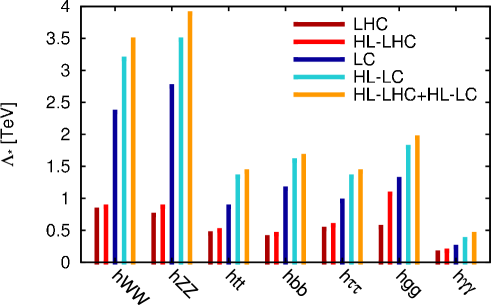
Figure 1: Effective scales $\Lambda_{\star}$ to be probed at various collider options, based on the precisions given in Tab. 1. For details, see Englert:2014uua .

The projected limits on $\Lambda_{\star}$ are summarized in Table 2. As can be inferred from the table the effective NP scales that can be probed in the Higgs sector range from several hundred GeV to maximum values beyond a TeV. The bounds on new particle masses $M$ exchanged in the Higgs vertex may, however, be reduced significantly by small couplings, $M\sim\Lambda_{\star}\sqrt{g^{2}/(16\pi^{2})}$, where $g$ generically denotes the NP coupling.

$\Lambda_{\ast}$ [TeV]	LHC	HL-LHC	LC	HL-LC	HL-LHC + HL-LC
$hWW$	0.82	0.87	2.35	3.18	3.48
$hZZ$	0.74	0.87	2.75	3.48	3.89
$htt$	0.45	0.50	0.87	1.34	1.42
$hbb$	0.39	0.44	1.15	1.59	1.66
$h\tau\tau$	0.52	0.58	0.96	1.34	1.42
$hgg$	0.55	1.07	1.30	1.80	1.95
$h\gamma\gamma$	0.15	0.18	0.24	0.36	0.44

Table 2: Effective NP scales $\Lambda_{\ast}$ extracted from the expected accuracy on Higgs couplings at present and future colliders given in Table 1. Taken from Englert:2014uua .

In case of non-linearly realized electroweak symmetry breaking (EWSB), the most general effective Lagrangian at ${\cal O}(p^{4})$ in a derivative expansion, focusing on cubic terms with at least one Higgs boson, assuming CP conservation and vector fields coupling to conserved currents, is given by Contino:2010mh ; Azatov:2012bz ; Alonso:2012px ; Buchalla:2013rka ; Brivio:2013pma ,

$${\cal L} = \,\frac{1}{2}\partial_{\mu}h\ \partial^{\mu}h-\frac{1}{2}m_{h}^{2}h^{2}-c_{3}\,\frac{1}{6}\,\left(\frac{3m_{h}^{2}}{v}\right)h^{3}-\sum_{\psi=u,d,l}m_{\psi^{(i)}}\,\bar{\psi}^{(i)}\psi^{(i)}\left(1+c_{\psi}\frac{h}{v}+\dots\right)$$ (1)

$$+m_{W}^{2}\,W^{+}_{\mu}W^{-\,\mu}\left(1+2c_{W}\,\frac{h}{v}+\dots\right)+\frac{1}{2}m_{Z}^{2}\,Z_{\mu}Z^{\mu}\left(1+2c_{Z}\,\frac{h}{v}+\dots\right)+\dots$$

$$+\left(\frac{\bar{c}_{WW}\,\alpha}{\pi}\,W_{\mu\nu}^{+}W^{-\mu\nu}+\frac{\bar{c}_{ZZ}\,\alpha}{2\pi}\,Z_{\mu\nu}Z^{\mu\nu}+\frac{\bar{c}_{Z\gamma}\,\alpha}{\pi}\,Z_{\mu\nu}\gamma^{\mu\nu}+\frac{\bar{c}_{\gamma\gamma}\,\alpha}{2\pi}\,\gamma_{\mu\nu}\gamma^{\mu\nu}+\frac{\bar{c}_{gg}\,\alpha_{s}}{12\pi}\,G_{\mu\nu}^{a}G^{a\mu\nu}\right)\frac{h}{v}$$

$$+\Big{(}\left(\bar{c}_{W\partial W}\,W^{-}_{\nu}D_{\mu}W^{+\mu\nu}+h.c.\right)+\bar{c}_{Z\partial Z}\,Z_{\nu}\partial_{\mu}Z^{\mu\nu}+\bar{c}_{Z\partial\gamma}\,Z_{\nu}\partial_{\mu}\gamma^{\mu\nu}\Big{)}\,\frac{h}{v}+\dots\;,$$

where $\psi$ denotes the fermion fields, $\alpha$ the EW and $\alpha_{s}$ the strong coupling. The EW and photon fields are described by $Z,W$ and $\gamma$, the gluon fields by $G$, with $a$ being the color index. The couplings $c_{i},\bar{c}_{i}$ can take arbitrary values and the Higgs boson $h$ need not be part of an electroweak doublet. The couplings are truly independent of other parameters that do not involve the Higgs boson. Applying the Lagrangian to the linear realization on the other hand, only 4 couplings between the Higgs boson $h$ and the vector bosons $V$ are independent of the other EW measurements Elias-Miro:2013mua ; Pomarol:2013zra . For a discussion of the physics implications, cf. Contino:2013kra . In the SM limit $c_{i}=1$ and $\bar{c}_{i}=0$.

III Composite Higgs Models

In Composite Higgs Models a light Higgs boson arises as a pseudo Nambu-Goldstone boson from a strongly-interacting sector Dimopoulos:1981xc ; Kaplan:1983fs ; Banks:1984gj ; Kaplan:1983sm ; Georgi:1984ef ; Georgi:1984af ; Dugan:1984hq , implying modified couplings compared to the SM. Such models are examples for EWSB based on a strong dynamics. In Giudice:2007fh an effective low-energy description of a Strongly Interacting Light Higgs Boson (SILH) has been given, which can be viewed as first term of the expansion in the compositeness parameter $\xi=\frac{v^{2}}{f^{2}}$, where $v\approx 246$ GeV is the VEV and $f$ the scale of the strong dynamics. The SILH Lagrangian is applicable in the vicinity of the SM limit, i.e. $\xi\to 0$, but for larger values of $\xi$ a resummation of the series in $\xi$ has to be performed. Explicit models built in five-dimensional warped space provide such a resummation: In the Minimal Composite Higgs Models (MCHM) discussed in Refs. Agashe:2004rs ; Contino:2006qr the global $SO(5)\times U(1)$ symmetry is broken down at the scale $f$ to $SO(4)\times U(1)$ on the infrared brane and to the SM group $SU(2)_{L}\times U(1)_{Y}$ on the ultraviolet brane. (For an MCHM implementing the antisymmetric representation ${\bf 10}$, see e.g. Gillioz:2013pba .) In these models the Higgs coupling modifications can be described by one single parameter, namely $\xi$. In the model, named MCHM4, of Agashe:2004rs the fermions are in the spinorial representation of $SO(5)$. Here all Higgs couplings are suppressed by the same universal factor $(1-\xi)^{1/2}$. This case is covered by the analysis of portal models. In MCHM5, the fermions are in the fundamental representation of $SO(5)$, and the couplings to massive gauge bosons $V=W,Z$ and the ones to fermions $f$ are modified by a different coefficient with respect to the SM,

$$1+\Delta_{V}=\sqrt{1-\xi}\approx 1-\frac{\xi}{2}\;,\quad 1+\Delta_{f}=\frac{1-2\xi}{\sqrt{1-\xi}}\approx 1-\frac{3\xi}{2}\;,$$ (2)

for $\xi\ll 1$. Table 3 shows the bounds on $\xi$, respectively the scale $f$, derived by assuming the Higgs coupling precisions given in Table 1.

$\xi$	LHC	HL-LHC	LC	HL-LC	HL-LHC+HL-LC
universal	0.076	0.051	0.008	0.0052	0.0052
non-universal	0.068	0.015	0.0023	0.0019	0.0019
$f$ [TeV]
universal	0.89	1.09	2.82	3.41	3.41
non-universal	0.94	1.98	5.13	5.65	5.65

Table 3: Derived bounds on the parameter $\xi=(v/f)^{2}$ and the Goldstone scale $f$ for various experimental set-ups. Taken from Englert:2014uua .

The computation of the Higgs boson decay widths and branching ratios can be performed with the Fortran code eHDECAY, Contino:2014aaa which has implemented different parametrisations of effective Lagrangians, the SILH approach, the non-linear realization of EWSB and the composite Higgs models MCHM4 and MCHM5. The program includes the most important higher-order QCD effects and in case of the SILH and composite Higgs parametrisation also the EW higher order corrections. The user furthermore has the possibility to turn off these EW corrections.

IV The Two-Higgs-Doublet Model and the MSSM

Two-Higgs-Doublet Models (2HDM) and the Minimal Supersymmetric extension of the SM (MSSM) are examples of NP, where the Higgs couplings are modified due to mixing effects. The 2HDM Lee:1973iz ; Flores:1982pr ; Gunion:1989we ; Branco:2011iw ; Gunion:2002zf belongs to the simplest extensions of the SM that allow to respect the experimentally measured $\rho$ parameter. The physical Higgs states are mixtures of the components of the two doublets $\phi_{1}$ and $\phi_{2}$. The scalar potential reads

$$V = m_{11}|\phi_{1}|^{2}+m_{22}^{2}|\phi_{2}|^{2}-m_{12}^{2}(\phi_{1}^{\dagger}\phi_{2}+\text{h.c})+\lambda_{1}|\phi_{1}|^{4}+\lambda_{2}|\phi_{2}|^{4}$$ (3)

$$+\lambda_{3}|\phi_{1}|^{2}|\phi_{2}|^{2}+\lambda_{4}|\phi_{1}^{\dagger}\phi_{2}|^{2}+\frac{1}{2}\lambda_{5}[(\phi_{1}^{\dagger}\phi_{2})^{2}+\text{h.c}]\,.$$

The neutral components of the Higgs doublets acquire VEVs $v_{1}$ and $v_{2}$, with the ratio defined as $\tan\beta=v_{2}/v_{1}$. They add up to $v^{2}=v_{1}^{2}+v_{2}^{2}$. The 2HDM features five Higgs bosons after EWSB, two neutral CP-even bosons $h^{0}$ and $H^{0}$, one CP-odd Higgs $A^{0}$ and two charged states $H^{\pm}$. The Higgs couplings to the fermions are different in specific realizations of the 2HDM. These arise by demanding a natural suppression of flavour-changing neutral currents, which is achieved by requiring that one type of fermions couples only to one Higgs doublet. It can be assured by imposing a global $\mathbb{Z}_{2}$ symmetry, under which $\phi_{1,2}\to\mp\phi_{1,2}$. This symmetry has been assumed in the potential Eq. (3), implying that all terms of the potential include an even power of each of the Higgs fields. There are four cases of possible couplings between the Higgs doublets and the fermions, that depend on the $\mathbb{Z}_{2}$ charge assignment Barger:1989fj .

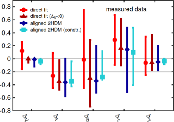
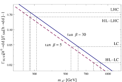
Figure 2: Left: Fits to the weak scale couplings and to the aligned 2HDM in terms of the light Higgs couplings based on the data from the 7 TeV run and an integrated luminosity of 4.6-5.1 fb^-1 and the 8 TeV run with 12-21 fb^-1, at 68% C.L., ATLAS and CMS combined Lopez-Val:2013yba . Right: Deviation of the MSSM tree-level decay width into down-type fermions from the SM value as function of $m_{A^{0}}$ for $\tan\beta=5$ and 30. For further details on $R_{t}$, see Englert:2014uua . Shown are the expected limits at the LHC, HL-LHC, LC and HL-LC.

In the aligned 2HDM, the Yukawa couplings of the two Higgs doublets are proportional to each other in flavour space. At tree level the aligned 2HDM is determined by five free parameters, including the mass of the charged Higgs boson, that contributes to the effective Higgs-photon coupling. Figure 2 (left) compares the extracted free Higgs couplings with the corresponding fit to the aligned 2HDM parameters, translated into the SM coupling deviations. For simplicity custodial symmetry, i.e. $\Delta_{Z}=\Delta_{W}\equiv\Delta V<1$ has been assumed. Note, that there are additional constraints due to non-standard Higgs searches and EW precision measurements as well as flavour constraints, in case the 2HDM is realized. These are taken into account in the cyan bands, while they have been ignored in the blue ones. The 2HDM has also been implemented in the Fortran code HDECAY Djouadi:1997yw ; Djouadi:2006bz ; Butterworth:2010ym to provide the Higgs decay widths and branching ratios including the state-of-the-art higher order QCD corrections and the off-shell Higgs decays Harlander:2013qxa .

The Higgs sector of the MSSM is a subgroup of the general 2HDM type-II where the up- and down-type fermions couple to $\phi_{2}$ and $\phi_{1}$, respectively. Furthermore, the quartic couplings are given in terms of the $SU(2)_{L}$ and $U(1)_{Y}$ gauge couplings. In the decoupling limit, where $H^{0},A^{0}$ and $H^{\pm}$ are heavy and $h^{0}$ behaves SM-like, the partial decay width of the latter into down-type fermions, normalized to the SM, scales with the pseudoscalar and the $Z$ boson masses, $\beta$ and the dominant supersymmetric radiative corrections $R_{t}$. Figure 2 (right) shows the deviation of this decay width in the MSSM from the SM as a function of $m_{A^{0}}$ for two different $\tan\beta$ values. It is proportional to the deviation in the Higgs coupling squared, and depending on the coupling precision achieved at the various colliders, limits on $m_{A^{0}}$ can be derived for a fixed value of $\tan\beta$.

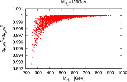
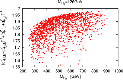
Figure 3: Left: Sum of the $H_{1}$ and $H_{2}$ (SM-like) gauge couplings squared. Right: Sum of their inverse Yukawa couplings squared. From Englert:2014uua .

V The NMSSM

The NMSSM (for recent reviews, see Maniatis:2009re ; Ellwanger:2009dp ) includes an additional singlet superfield and features 7 Higgs bosons after EWSB, three neutral CP-even ones $H_{1,2,3}$, two neutral CP-odd bosons $A_{1,2}$ and two charged Higgs bosons $H^{\pm}$. Due to the large number of parameters entering the tree-level Higgs sector, there are more possibilities to achieve an NMSSM scenario compatible with the present LHC data (see, e.g. King:2012is ; King:2012tr ; King:2014xwa ). At the same time it becomes more difficult to constrain a single parameter or a subset of the parameters based on the coupling measurements alone. However, the latter may allow to reveal if the possibly discovered new Higgs particles belong to the MSSM or the NMSSM, in case only three have been discovered and not all of them are CP-even. For the NMSSM this would reveal itself in the violation of the coupling sum rules for the scalar couplings to the gauge bosons,

$$\sum_{i=1}^{3}g_{H_{i}VV}^{2}=1\;,$$ (4)

and for the couplings to the top and bottom quarks,

$$\frac{1}{\sum_{i=1}^{3}g_{H_{i}tt}^{2}}+\frac{1}{\sum_{i=1}^{3}g_{H_{i}bb}^{2}}=1\;.$$ (5)

Figure 3 shows the scenarios with $H_{2}$ being SM-like from a scan over the NMSSM parameter range, which are in accordance with the LHC Higgs data. Assuming that only the two lightest CP-even Higgs bosons have been discovered, the left plot shows as a function of $M_{H_{3}}$ the violation of the vector coupling sum rule for $H_{1}$ and $H_{2}$ and the right plot the violation of the Yukawa coupling sum rule. The sums can deviate by up to a factor of two in case of the fermion couplings. While the precise determination of the Higgs couplings will allow to distinguish the MSSM from the NMSSM it will be difficult to deduce the mass of the unobserved third Higgs boson from the pattern of the violation of the sum rules. The larger number of parameters entering the Higgs sector does not allow to derive a unique correlation between the coupling values and the scale of NP. In this case a global scan has to be performed to pin down the underlying NP scale.

VI Conclusion

The precise investigation of the Higgs properties opens a unique window to NP scales beyond the direct reach of present colliders. It has been shown for some archetypal BSM scenarios that Higgs precision data can be sensitive to scales ranging from a few hundred GeV in weakly coupled models up to multi-TeV scales for models based on strong dynamics.

- (1) ATLAS Collaboration, G. Aad et al., Phys.Lett. B716, 1 (2012), 1207.7214.
- (2) CMS Collaboration, S. Chatrchyan et al., Phys.Lett. B716, 30 (2012), 1207.7235.
- (3) M. Kramer and M. Muhlleitner, Nucl.Part.Phys.Proc. 261-262, 246 (2015), 1501.06658.
- (4) M. Gouzevitch, A. Kaczmarska, M. Muhlleitner, and K. Turzynski, PoS DIS2014, 003 (2014).
- (5) C. Englert et al., J.Phys. G41, 113001 (2014), 1403.7191.
- (6) M. Muhlleitner, (2014), 1410.5093.
- (7) C. Burges and H. J. Schnitzer, Nucl.Phys. B228, 464 (1983).
- (8) C. N. Leung, S. Love, and S. Rao, Z.Phys. C31, 433 (1986).
- (9) W. Buchmuller and D. Wyler, Nucl.Phys. B268, 621 (1986).
- (10) B. Grzadkowski, M. Iskrzynski, M. Misiak, and J. Rosiek, JHEP 1010, 085 (2010), 1008.4884.
- (11) R. Lafaye, T. Plehn, M. Rauch, D. Zerwas, and M. Duhrssen, JHEP 0908, 009 (2009), 0904.3866.
- (12) M. Klute, R. Lafaye, T. Plehn, M. Rauch, and D. Zerwas, Phys.Rev.Lett. 109, 101801 (2012), 1205.2699.
- (13) T. Plehn and M. Rauch, Europhys.Lett. 100, 11002 (2012), 1207.6108.
- (14) R. Contino, C. Grojean, M. Moretti, F. Piccinini, and R. Rattazzi, JHEP 1005, 089 (2010), 1002.1011.
- (15) A. Azatov, R. Contino, and J. Galloway, JHEP 1204, 127 (2012), 1202.3415.
- (16) R. Alonso, M. Gavela, L. Merlo, S. Rigolin, and J. Yepes, Phys.Lett. B722, 330 (2013), 1212.3305.
- (17) G. Buchalla, O. Cat , and C. Krause, Nucl.Phys. B880, 552 (2014), 1307.5017.
- (18) I. Brivio et al., JHEP 1403, 024 (2014), 1311.1823.
- (19) J. Elias-Miro, J. Espinosa, E. Masso, and A. Pomarol, JHEP 1311, 066 (2013), 1308.1879.
- (20) A. Pomarol and F. Riva, JHEP 1401, 151 (2014), 1308.2803.
- (21) R. Contino, M. Ghezzi, C. Grojean, M. Muhlleitner, and M. Spira, JHEP 1307, 035 (2013), 1303.3876.
- (22) S. Dimopoulos and J. Preskill, Nucl.Phys. B199, 206 (1982).
- (23) D. B. Kaplan and H. Georgi, Phys.Lett. B136, 183 (1984).
- (24) T. Banks, Nucl.Phys. B243, 125 (1984).
- (25) D. B. Kaplan, H. Georgi, and S. Dimopoulos, Phys.Lett. B136, 187 (1984).
- (26) H. Georgi, D. B. Kaplan, and P. Galison, Phys.Lett. B143, 152 (1984).
- (27) H. Georgi and D. B. Kaplan, Phys.Lett. B145, 216 (1984).
- (28) M. J. Dugan, H. Georgi, and D. B. Kaplan, Nucl.Phys. B254, 299 (1985).
- (29) G. Giudice, C. Grojean, A. Pomarol, and R. Rattazzi, JHEP 0706, 045 (2007), hep-ph/0703164.
- (30) K. Agashe, R. Contino, and A. Pomarol, Nucl.Phys. B719, 165 (2005), hep-ph/0412089.
- (31) R. Contino, L. Da Rold, and A. Pomarol, Phys.Rev. D75, 055014 (2007), hep-ph/0612048.
- (32) M. Gillioz, R. Grober, A. Kapuvari, and M. Muhlleitner, JHEP 1403, 037 (2014), 1311.4453.
- (33) R. Contino, M. Ghezzi, C. Grojean, M. Muhlleitner, and M. Spira, Comput.Phys.Commun. 185, 3412 (2014), 1403.3381.
- (34) T. Lee, Phys.Rev. D8, 1226 (1973).
- (35) R. A. Flores and M. Sher, Annals Phys. 148, 95 (1983).
- (36) J. F. Gunion, H. E. Haber, G. L. Kane, and S. Dawson, Front.Phys. 80, 1 (2000).
- (37) G. Branco et al., Phys.Rept. 516, 1 (2012), 1106.0034.
- (38) J. F. Gunion and H. E. Haber, Phys.Rev. D67, 075019 (2003), hep-ph/0207010.
- (39) V. D. Barger, J. Hewett, and R. Phillips, Phys.Rev. D41, 3421 (1990).
- (40) D. Lopez-Val, T. Plehn, and M. Rauch, JHEP 1310, 134 (2013), 1308.1979.
- (41) A. Djouadi, J. Kalinowski, and M. Spira, Comput.Phys.Commun. 108, 56 (1998), hep-ph/9704448.
- (42) A. Djouadi, M. Muhlleitner, and M. Spira, Acta Phys.Polon. B38, 635 (2007), hep-ph/0609292.
- (43) J. Butterworth et al., (2010), 1003.1643.
- (44) R. Harlander, M. Muhlleitner, J. Rathsman, M. Spira, and O. Stal, (2013), 1312.5571.
- (45) M. Maniatis, Int.J.Mod.Phys. A25, 3505 (2010), 0906.0777.
- (46) U. Ellwanger, C. Hugonie, and A. M. Teixeira, Phys.Rept. 496, 1 (2010), 0910.1785.
- (47) S. King, M. Muhlleitner, and R. Nevzorov, Nucl.Phys. B860, 207 (2012), 1201.2671.
- (48) S. King, M. Muhlleitner, R. Nevzorov, and K. Walz, Nucl.Phys. B870, 323 (2013), 1211.5074.
- (49) S. King, M. Muhlleitner, R. Nevzorov, and K. Walz, Phys.Rev. D90, 095014 (2014), 1408.1120.