Extending quantum mechanics entails extending special relativity

Abstract

The complementarity between signaling and randomness in any communicated resource that can simulate singlet statistics is generalized by relaxing the assumption of free will in the choice of measurement settings. We show how to construct an ontological extension for quantum mechanics (QM) through the oblivious embedding of a sound simulation protocol in a Newtonian spacetime. Minkowski or other intermediate spacetimes are ruled out as the locus of the embedding by virtue of hidden influence inequalities. The complementarity transferred from a simulation to the extension unifies a number of results about quantum nonlocality, and implies that special relativity (SR) has a different significance for the ontological model and for the operational theory it reproduces. Only the latter, being experimentally accessible, is required to be Lorentz covariant. There may be certain Lorentz non-covariant elements at the ontological level, but they will be inaccessible at the operational level in a valid extension. Certain arguments against the extendability of QM, due to Conway and Kochen (2009) and Colbeck and Renner (2012), are attributed to their assumption that the spacetime at the ontological level has Minkowski causal structure.

I Introduction

Bell’s theorem proves that quantum nonlocality cannot be reproduced by any local realistic model Bell (1964). A simple instance of nonlocality is demonstrated by the quantum violation of the CHSH inequality Clauser et al. (1969)

$$\Lambda(\textbf{P})=\sum_{a,b}(-1)^{a\overline{b}}E(a,b)\leq 2,$$ (1)

with inputs $a,b\in\{0,1\}$ and the expectation value $E(a,b)\equiv P(x=y|ab)-P(x\neq y|ab)$, where the respective outputs are $x,y\in\{0,1\}$. Here $\overline{b}\equiv b\oplus 1$, where $\oplus$ indicates addition modulo 2. Bell’s theorem places no restriction on how much must be given up in a hidden variable (HV) model or “extension”. Bell’s result has been strengthened by the relaxing of localism Leggett (2003); Gröblacher et al. (2007), and further strengthened recently through the ruling out of any (nontrivial) local part Barrett et al. (2006); Branciard et al. (2008); Colbeck and Renner (2008).

The above works entail that any HV model of singlet correlations must be entirely nonlocal. Two recent works, invoking special relativity (SR) and a certain version of free will, present arguments that would also rule out deterministic nonlocal extensions Conway. and Kochen. (2006); *CK09 and indeterministic nonlocal extensions also Colbeck and Renner (2011). On this basis, they argued that nonlocal extensions of QM like Bohmian Bohm (1952a); *Boh52b and GRW collapse models Ghirardi et al. (1986) are incompatible with with SR and free will.

These conclusions were contested Bassi and Ghirardi (2007); Tumulka (2007); Goldstein et al. (2010); Suarez (2010) on the basis of two broad grounds: (a) that Bohmian and GRW collapse theories are already known to be observationally compatible with SR. In the case of the former, this has been known since Bohm’s original works and also from Bell’s writings Bell (1987). As regards their ontological compatibility with SR, cf. Suarez (2010); Tumulka (2006a); *Tum06b; Dürr et al. (2014); Bedingham et al. (2014). Thus these models have no obvious obstacle to admitting free will; (b) that FW and no-signaling are logically independent, so that invoking FW to rule out predictively superior extensions is untenable Ghirardi and Romano (2013a, b).

This conflict illustrates that the “tension” between SR and quantum nonlocality is still not unequivocally resolved. In this work, we provide a resolution to this conflict by identifying the different assumptions behind the conflicting claims.

Our approach to the resolution will be through the following four steps, an expansion of which is given in the overview presented in Section II. In the first step, we clarify (Section III) that nonlocal correlations must be viewed from two levels or layers: the operational level accessible to experimentalists and the ontological level, where the HV’s, by definition inaccessible and unknowable, live Spekkens (2005); Cavalcanti and Wiseman (2012). In particular, we define unpredictability and (operational) no-signaling as operational concepts, having indeterminism and ontological no-signaling as their ontological counterparts. In Section IV, we define free will as appropriate to Bell-type experiments, and introduce the concept of spontaneity, as the operational equivalent of free will. We clarify in this first step that only operational concepts, and not their ontological counterparts, are required to be Lorentz covariant, since only operational quantities are experimentally accessible. For terminological clarity, we propose the concepts of randomness, signaling and freedom as the level-neutral counterparts of the three operational/ontological concepts discussed above.

As the second step in our argument, we present a protocol for simulating singlet statistics (Section V). A complementarity of the signaling and randomness of resources used in the protocol, as modified by relaxing the assumption of free will, is formulated in Section VI.

As the third step, we present in Section VII an explicit procedure to convert any sound simulation protocol into a valid ontological extension of QM. There is a two-fold subtlety about this conversion: (a) The protocol must be embedded in a Newtonian (and not Minkowski) spacetime; (b) The embedding must be oblivious, meaning that certain simulation parameters will map to the ontological theory, and hence must be unknowable to physical observers, Alice and Bob.

This exercise will allow us to clarify that an extension of QM may contain ontological features that are Lorentz non-covariant. However, these will either be suitably averaged out or physically inaccessible, such that the resulting operational theory will conform to SR, assuming the soundness of the simulation protocol.

As the fourth and last step in our approach, we show (Section VIII) how the freewill-relaxed randomness-signaling complementarity of simulation resources carries over to the ontological extension under the embedding procedure. All the above stronger forms of Bell inequalities will be derived as consequences of this transplanted complementarity in the context of singlet statistics. Here we will finally be in a position to revisit and unpack the above mentioned debate in the literature regarding free will, no-signaling and unextendability of QM. We conclude in Section IX.

II Overview of results

In view of the fact that the problem dealt with is fraught with conceptual difficulties, we present in this section an outline of the arguments in this work. This outline essentially expands the four steps mentioned above.

II.1 Definitions: Operational and ontological levels

It is known that two levels of description come into play in the description of nonlocality Spekkens (2005); Cavalcanti and Wiseman (2012): the operational or observational level and the ontological or HV level. Here we wish to stress that these two levels are constrained differently by relativistic causality. For our purpose, it suffices to characterize the correlations in terms of three concepts or resources, which must be defined at both the operational and ontological levels. The three concepts are randomness, (no-)signaling and freedom (in measurement settings) in a correlation, all three of which must be specified at the operational and ontological levels. Their definitions are given in Sections III and IV.

We list the operational and ontological equivalents of these three concepts in Table 1.

Level-neutral	Operational	Ontological
Concept	quantity	counterpart
Randomness	unpredictability	indeterminism
No-signaling	operational	ontological
	no-signaling	no-signaling
Freedom	spontaneity	free will

Table 1: Operational and ontological equivalents in the context of quantum nonlocal correlations. Only operational quantities are required to be Lorentz covariant.

The concepts ontological no-signaling and operational no-signaling in Table 1 are close to the concepts of locality and signaling locality in Ref. Cavalcanti and Wiseman (2012), and similarly the concepts of unpredictability and indeterminism in Table 1 parallel the like-named concepts in Ref. Cavalcanti and Wiseman (2012). The concept of spontaneity is introduced here is the operational equivalent of free will Hall (2010a).

In each case, the operational quantity is obtained by averaging over the ontic or underlying state $\lambda$ of the system. As the experimentally accessible variables, only the operational quantities in Table 1 are required to amenable to a covariant description. By contrast, ontological variables are by definition unknowable and inaccessible, and thus they are not compelled by relativistic causality to satisfy Lorentz covariance. For example, an extension may violate ontological no-signaling, but this will not matter provided the theory reproduced on the operational level satisfies operational no-signaling.

II.2 Result 1: Freedom-relaxed complementarity

It will be convenient to think of a protocol $\mathfrak{S}$ for simulating nonlocality (in the context of singlet statistics) as two-layered: the base layer consisting of the input and output random variables $A,B,X$ and $Y$ of Alice and Bob in a practical experiment; and the meta-layer consisting of the classical randomness (denoted $\chi$ and $\chi^{+}$ here) that Alice and Bob pre-share in the simlation, and the resource $\mathcal{R}$ that Alice communicates to Bob during the simulation run. In accordance with this two-layering, it will sometimes be convenient to refer to $A,B,X,Y$ as the base data, and to $\mathcal{R},\chi,\chi^{+}$ as the meta data.

It is known that the resource $\mathcal{R}$ consisting of a one-bit signal Toner and Bacon (2003) or of a single Popescu-Rohrlich (PR) box Cerf et al. (2005) (which is non-signaling but with maximal local randomness) suffices to simulate the nonlocal statistics of a singlet. More generally, the communicated resource $\mathcal{R}$ shows a complementarity between signaling $S_{R}$ and local randomness $I_{R}$ Hall (2010b); Kar et al. (2011); Aravinda and Srikanth (2015a). Our first result is to generalize this complementarity by relaxing the assumption of experimenters’ free will $F$ Hall (2010a).

Reducing freedom $F$ relaxes the above complementaristic constraint on $S_{R}$ and $I_{R}$, until (at $F=\frac{2}{3}$) there is no bound on these two quantities, i.e., the correlations can be reproduced using a mixture of local-deterministic correlations. Under maximal freedom, the complementarity has the form:

$$S_{R}+2I_{R}\geq 1$$ (2)

for singlet simulation, a result proved in Section VI. Complementarity (2) implies that under the assumption of maximal freedom, the amount of randomness and signaling cannot both be arbitrarily low in resource $\mathcal{R}$ that is suitable to simulate singlet statistics.

II.3 Result 2: Elevating a simulation protocol to an ontological model via Oblivious embedding in a Newtonian spacetime

We show how to elevate protocol $\mathfrak{S}$ to an ontological model by letting “Nature run $\mathfrak{S}$” in spacetime. This seems intuitively clear, but it would appear that communicating resource $\mathcal{R}$ in spacetime would violate no-signaling and hence relativistic causality in the case of spacelike separated measurements. Key to seeing that this is not so, is to observe that precisely the base layer of protocol $\mathfrak{S}$ is mapped to the operational theory, whereas the meta layer gets mapped to the ontological model. Accordingly, we have the following recipe for mapping of data in $\mathfrak{S}$ to variables in spacetime:

$${\rm Base~{}data~{}of~{}}\mathfrak{S} \longrightarrow {\rm operational~{}variables}$$

$${\rm Meta~{}data~{}of~{}}\mathfrak{S} \longrightarrow {\rm ontological~{}variables}$$ (3)

Therefore, the type of no-signaling violated during the communication of $\mathcal{R}$ is ontological. Since ontological variables are by definition inaccessible to Alice and Bob (the observers in the operational theory), no violation of relativistic causality occurs at the operational level. On the other hand, the base data by itself is consistent with no-signaling (in that mutual information $I(A:Y)=0$, etc.), and thus there is no difficulty in mapping this data to operational variables.

Obviously, the spacetime in which ontological elements live cannot be governed by SR, but instead should be governed by a suitable “ontological extension of SR” (SRX). A SRX is a relativity theory in which the causal structure of SR is replaced by another one (appropriate for quantum nonlocal phenomena) in which at each event e, the causally connected region strictly encompasses the light cones of SR. (Other details of SR are not germane here.) A SRX is a kind of $v$-causal model of the type proposed in Ref. Salart et al. (2008). Within this framework (of deriving an ontological model from a simulation protocol), it turns out that the only allowed SRX is the one equipped with Galilean invariance, i.e., the Newtonian spacetime, because for any other SRX, one can always produce an experimental configuration that would predict a breakdown in the quantum correlations. Hidden influence inequalities Salart et al. (2008) can be constructed that make use of this breakdown for superluminal signaling at the operational level.

This conclusion does not automatically apply to extensions of QM that cannot be analyzed manifestly as simulation protocols embedded in spacetime, i.e., in the pattern of Eq. (3). In such cases, Lorentz covariance may indeed hold for elements recognized as ontological in the extension, cf. Refs. Suarez (2010); Tumulka (2006a); *Tum06b; Dürr et al. (2014); Bedingham et al. (2014) as regards GRW and Bohmian models. In this light, our result can broadly be interpreted as showing that for any model of a nonlocal theory like QM, under the assumption of free will, there would be fundamental influences and fundamental correlations not conforming to the lightcone structure.

We thereby have a procedure to elevate any protocol $\mathfrak{S}$ to an ontological extension of (a fragment of) QM, by embedding $\mathfrak{S}$ in a SRX, as described above. This shows in a simple way that extension of this type will contain some ontological elements that aren’t Lorentz covariant. But the physical agents Alice and Bob will be oblivious to (i.e., unable to access) them. Thus, conformance to no-signaling is automatically guaranteed at the operational level.

II.4 Discussion: SR and complementarity in the derived extension

The signaling and randomness in the meta data $\mathcal{R}$ (discussed above in Section II.2) is transferred from the simulation scenario to the spacetime scenario under the embedding scheme (discussed in Section II.3). By virtue of assignment (3), we then have at the ontological level:

$$S_{R} \rightarrow S_{\lambda}$$

$$I_{R} \rightarrow I_{\lambda}.$$ (4)

With this identification, Eq. (2) becomes:

$$S_{\lambda}+2I_{\lambda}\geq 1,$$ (5)

i.e., a complementarity between ontological signaling and indeterminism. The is a stronger form of Bell’s theorem, which only says $S_{\lambda}+2I_{\lambda}>0$. By identifying meta data $\chi,\chi^{+}$ with the underlying ontological state, we can identify freedom $F$ with free will (and will use the same symbol, since there is no confusion). The complementarity (5) can be used to obtain equivalent derivations of the various stronger forms of Bell inequalities mentioned earlier, namely Leggett (2003); Gröblacher et al. (2007); Barrett et al. (2006); Branciard et al. (2008); Colbeck and Renner (2008), as well as the mathematical essence of Refs. Conway. and Kochen. (2006); *CK09 and Colbeck and Renner (2011).

The operational theory can be considered as a “trivial ontology” by setting the signaling $S_{\lambda}^{\rm triv}\equiv S=0$, from which and Eq. (5) it follows that $I^{\rm triv}_{\lambda}\equiv I=\frac{1}{2}$. In other words, the operational theory must contain maximum unpredictability. Ontologically, we can have predictive superiority, i.e., $I_{\lambda}<\frac{1}{2}$, and from Eq. (5), we find $S_{\lambda}>0$. This means that any predictively superior extension will contain signaling at the ontological level, which can (as indicated in Section II.3) coexist peacefully with no-signaling at the operational level.

We stress that this conclusion was already reached by the proponants of Bohmian mechanics and GRW models with respect to their own models. What is new to our work is to identify for the class of ontological models based on a protocol for simulating quantum nonlocality, which elements in a predictively superior extension of QM are necessarily Lorentz-covariant and which elements may be non-covariant: namely, the operational and ontological, respectively. As one particular application of this result, our work gives a general and simple explanation of why the technical no-go results of the type Conway. and Kochen. (2006); *CK09; Colbeck and Renner (2011) cannot be interpreted as prohibiting such extensions on grounds of relativity, essentially because the non-covariance that they identify pertains to the ontological elements for this class of extensions.

III Resources in operational and ontological theories: signaling and randomness

By an “operational theory” we mean a theory characterized by physical measurements and observations by one or more parties, outcomes and the corresponding conditional correlations. An operational theory may contain counterintuitive features like non-signaling nonlocality, for which an “ontological model”, such as a HV theory, attempts to provide a more intuitive and classical-like explanation using variables that may not be directly accessible physically.

III.1 Signaling: operational and ontological

A bipartite correlation $\textbf{P}\equiv P_{XY|AB}$ generated by measurements in an operational theory, is non-signaling if

$$P_{X|AB} = P_{X|A},$$

$$P_{Y|AB} = P_{Y|B}.$$ (6)

where $A$ and $X$ (resp., $B$ and $Y$) are Alice’s (resp., Bob’s) input and output spacetime-labelled random variables (abbreviated to SVs). By relativity considerations, Eq. (6) must hold if $A$ and $B$ are spacelike separated and freely chosen.

Now suppose we extend conditions (6), requiring no-signaling additionally in a HV theory. Then we may require:

$$P_{X|AB\lambda} = P_{X|A\lambda},$$

$$P_{Y|AB\lambda} = P_{Y|B\lambda},$$ (7)

where $\lambda$ is the HV describing the ontic state in the underlying ontological theory. Eq. (7) is a version of the ontological no-signaling condition. If Alice and Bob choose their measurement settings freely, then it is not necessary for this condition to be satisfied. This point is crucial here, in that the nay-sayers in the above debate treat it at par with operational no-signaling.

Instead, what is necessary by virtue of requiring SR to hold in the operational theory, is the following: If $\rho(\lambda|AB)$ represents the probability distribution of $\lambda$ conditioned on the inputs in the operational theory, then we require that $P_{X|AB}\equiv\int\rho(\lambda|AB)P_{X|AB\lambda}d\lambda$ and $P_{Y|AB}\equiv\int\rho(\lambda|AB)P_{Y|AB\lambda}d\lambda$ should satisfy the operational no-signaling conditions (6), if Alice and Bob have full free will, i.e., $\rho(\lambda|AB)=\rho(\lambda)$.

As we show later, the violation of ontological no-signaling is necessary for non-trivial extensions of QM. Recognizing this beneficial aspect of ontological signaling is key to resolving the aforementioned debate.

$ab$	$\textbf{d}^{0_{1}}$	$\textbf{d}^{1_{1}}$	$\textbf{d}^{2_{1}}$	$\textbf{d}^{3_{1}}$	$\textbf{d}^{4_{1}}$	$\textbf{d}^{5_{1}}$	$\textbf{d}^{6_{1}}$	$\textbf{d}^{7_{1}}$
00	00	11	00	11	00	11	00	11
01	00	11	00	11	00	00	11	11
10	01	01	10	10	10	01	10	01
11	00	00	11	11	00	00	11	11

Table 2: The complete list of deterministic 1-bit boxes $\textbf{d}^{j_{1}}$ that violate Ineq. (1) to its algebraic maximum of +4. Every 1-bit box $\textbf{d}^{j_{1}}$ is paired with an “anti-box”, e.g., $\textbf{d}^{0_{1}}$ with $\textbf{d}^{3_{1}}$, with complementary outputs. Together with the deterministic correlations of Table 3, these constitute the full set of extreme points for the signaling polytope $\mathfrak{F}^{P}$.

If the condition for operational no-signaling (6) or for ontotological no-signaling (7) is violated, the resultant operational signal or ontological signal can be quantified in a variety of ways. One such is described below. In the two-input-two-output case, the operational signal from Alice to Bob ($S^{A\rightarrow B}$) and Bob to Alice ($S^{B\rightarrow A}$) can be quantified as

$$S^{A\rightarrow B} = \sup_{b}|P_{y|0,b}-P_{y|1,b}|$$

$$S^{B\rightarrow A} = \sup_{a}|P_{x|a,0}-P_{x|a,1}|,$$ (8)

where $P_{x|a,b}$ (resp., $P_{y|a,b}$) is Alice’s (resp. Bob’s) marginal distribution. The operational signal is quantified as

$$S=\max\{S^{A\rightarrow B},S^{B\rightarrow A}\},$$ (9)

with the condition $S=0$ implying (6). In general, $0\leq S\leq 1$ and specifically $S\leq C$, where $C$ is the communication cost of correlation P Aravinda and Srikanth (2015b). If the operational no-signaling condition (6) is violated, then $S>0$.

In analogy with definition (9), the ontological signal $S_{\lambda}$ can be quantified by replacing $P_{x|ab}$ and $P_{y|ab}$ in (9) by $P_{x|ab\lambda}$ and $P_{y|ab\lambda}$, where the latter two quantities are Alice’s and Bob’s marginal distribution in the ontic state $\lambda$. The condition $S_{\lambda}=0$ implies the ontological no-signaling condition (7). In general, $0\leq S_{\lambda}\leq 1$ Aravinda and Srikanth (2015b). We only require that $S=0$. If the operational theory contains correlation P given by a PR box Popescu and Rohrlich (1994), then $S_{\lambda}=1$ and $S=0$.

As an illustration of ontological signaling leading to operational no-signaling, consider the determinsitic distributions given in Table 2 as ontic states $\lambda$ in an underlying theory. As each of them requires 1 bit of communication to be simulated, we will refer to them as “1-bit boxes”, denoted $\textbf{d}^{j_{1}}$ ($j=0,1,2\cdots,7$).

An example of a 1-bit box is $\textbf{d}^{0_{1}}$, which denotes the probability distribution $d^{0_{1}}_{xy|ab}\equiv\delta^{0}_{x}\delta_{y}^{a\cdot(b\oplus 1)}$. We can obtain the PR box at the operational level by uniformly mixing “boxes” $\lambda=\textbf{d}^{0_{1}}$ and $\lambda=\textbf{d}^{3_{1}}$. In this case, there is an ontological signal from Alice to Bob in both individual cases of $\lambda$ in violation of (7). However, in the PR box realized at the operational level, the operational no-signaling condition (6) is satisfied. Conversely, ontologically non-signaling ontic states can lead to operational signaling, when the free will of Alice or Bob is reduced through non-trivial $\rho(\lambda|AB)$, as discussed in Section IV.

III.2 Unpredictability and indeterminism

We denote by $I$ the degree of unpredictability, or local randomness in the operational theory, generated by measurement of either observer:

$$I\equiv\sup_{a,b}\min_{z}\{P_{z|a,b}\},$$ (10)

where $z$ is the outcome on any one of the parties Hall (2010b). In general, $0\leq I\leq\frac{1}{2}$. The ontological counterpart of $I$, which is indeterminism, denoted $I_{\lambda}$, is defined analogously, with additional conditioning on $\lambda$:

$$I_{\lambda}\equiv\sup_{a,b}\min_{z}\{P_{z|a,b,\lambda}\}.$$ (11)

A deterministic system is predictable, but the converse is not true. For the model for the PR box mentioned earlier, we find $I=\frac{1}{2}$ and $I_{\lambda}=0$. Thus the operational theory is maximally unpredictable, but the underlying theory is fully deterministic.

IV Free will and spontaneity

The question of what free will is, and whether it exists in Nature, has been debated for centuries in philosophy Hanaan and Srikanth (2015). In the context of Bell tests, free will is taken to be the freedom or uncorrelatedness of the observers’ choice of measurement settings from factors lying to the past. Two relevant and sometimes contentious questions here are: What factors to be free from? What is the scope of the past? The answers depend on the type of freedom in question: whether it is operational or ontological. Following convention, we identify the ontological variety with the term “free will”.

Ref. Hall (2010a) defines free will $F$ as a measure of Alice’s and Bob’s choices being uncorrelated with the underlying state $\lambda$:

$$F\equiv 1-\frac{1}{2}\left(\sup_{a,a^{\prime},b,b^{\prime}}\int d\lambda|\rho(\lambda|a,b)-\rho(\lambda|a^{\prime},b^{\prime})|\right),$$ (12)

where $\rho(\lambda|a,b)$ is the probability distribution of $\lambda$ conditioned on input $a,b$. Free will so quantified satisfies the bound $0\leq F\leq 1$.

Even with a reduction of free will by a fraction $\frac{1}{3}$, the CHSH inequality can be violated to the algebraic maximum using a local-deterministic model. For the eight local-deterministic boxes with $\Lambda=+2$, given in Table 3, this is proven below.

As the correlations in Table 3 require zero bits of communication to be simulated, we shall refer to them as “0-bit boxes”, and denote them by $\textbf{d}^{j_{0}}$ ($j=0,1,2\cdots$). An example for a 0-bit box is $\textbf{d}^{2_{0}}$, which represents the probability distribution $d^{2_{0}}_{xy|ab}\equiv\delta^{0}_{x}\delta^{b\oplus 1}_{y}$, where $\delta^{\mu}_{\nu}$ is the Dirac delta function.

$ab$	$\textbf{d}^{0_{0}}$	$\textbf{d}^{1_{0}}$	$\textbf{d}^{2_{0}}$	$\textbf{d}^{3_{0}}$	$\textbf{d}^{4_{0}}$	$\textbf{d}^{5_{0}}$	$\textbf{d}^{6_{0}}$	$\textbf{d}^{7_{0}}$
00	00	00	01	11	00	10	11	11
01	00	00	00	10	01	11	11	11
10	00	10	01	01	10	10	01	11
11	00	10	00	00	11	11	01	11

Table 3: The complete list of deterministic 0-bit boxes $\textbf{d}^{j_{0}}$, for which $\Lambda=+2$ in Ineq. (1). The first column lists the inputs, while the other columns give the outputs corresponding to the box.

We consider a method for reduction of free will effected by requiring that Alice’s and Bob’s choice of inputs will depend on $\lambda=\textbf{d}^{j_{0}}$ according to:

$$\rho(ab|\lambda)=\begin{matrix}\textbf{d}^{0_{0}}&\textbf{d}^{1_{0}}&\textbf{d}^{2_{0}}&\textbf{d}^{3_{0}}&\textbf{d}^{4_{0}}&\textbf{d}^{5_{0}}&\textbf{d}^{6_{0}}&\textbf{d}^{7_{0}}\\ \hline\cr\beta&\beta&\alpha&\beta&\beta&\alpha&\beta&\beta\\ \beta&\beta&\beta&\alpha&\alpha&\beta&\beta&\beta\\ \alpha&\beta&\beta&\beta&\beta&\beta&\beta&\alpha\\ \beta&\alpha&\beta&\beta&\beta&\beta&\alpha&\beta\\ \end{matrix}$$ (13)

where the real numbers $\alpha,\beta\geq 0$ and by normalization $\alpha+3\beta=1$. The rows correspond sequentially to inputs $ab=00,01,10,11$. Here $\alpha$ must be less than the unbiased probability of $\frac{1}{4}$ to suppress the input for which $E(a,b)\neq(-1)^{a\overline{b}}$ in the contribution to the CHSH inequality (1).

Letting each $ab$ and each $\lambda=\textbf{d}^{j_{0}}$ be uniformly probable, by Bayesian arguments we have from Eq. (13)

$$\rho(\lambda|ab)=\begin{matrix}\textbf{d}^{0_{0}}&\textbf{d}^{1_{0}}&\textbf{d}^{2_{0}}&\textbf{d}^{3_{0}}&\textbf{d}^{4_{0}}&\textbf{d}^{5_{0}}&\textbf{d}^{6_{0}}&\textbf{d}^{7_{0}}\\ \hline\cr\frac{\beta}{2}&\frac{\beta}{2}&\frac{\alpha}{2}&\frac{\beta}{2}&\frac{\beta}{2}&\frac{\alpha}{2}&\frac{\beta}{2}&\frac{\beta}{2}\\ \frac{\beta}{2}&\frac{\beta}{2}&\frac{\beta}{2}&\frac{\alpha}{2}&\frac{\alpha}{2}&\frac{\beta}{2}&\frac{\beta}{2}&\frac{\beta}{2}\\ \frac{\alpha}{2}&\frac{\beta}{2}&\frac{\beta}{2}&\frac{\beta}{2}&\frac{\beta}{2}&\frac{\beta}{2}&\frac{\beta}{2}&\frac{\alpha}{2}\\ \frac{\beta}{2}&\frac{\alpha}{2}&\frac{\beta}{2}&\frac{\beta}{2}&\frac{\beta}{2}&\frac{\beta}{2}&\frac{\alpha}{2}&\frac{\beta}{2}\\ \end{matrix}.$$ (14)

Applying this data to the discrete version of definition (12) we find

$$F=1-|\alpha-\beta|=\frac{2+4\alpha}{3}.$$ (15)

Further, from Table 3 and Eq. (14), we find

$$P_{xy|ab}=\left\{\begin{array}[]{l||l|l|l|l}ab=00&3\beta/2&\alpha/2&\alpha/2&3\beta/2\\ \hline\cr ab=01&3\beta/2&\alpha/2&\alpha/2&3\beta/2\\ \hline\cr ab=10&\alpha/2&3\beta/2&3\beta/2&\alpha/2\\ \hline\cr ab=11&3\beta/2&\alpha/2&\alpha/2&3\beta/2,\\ \end{array}\right.$$ (16)

where each row represents a single input $ab$, and the columns represent the outputs 00, 01, 10 and 11. We denote the correlation in Eq. (16) by $\textbf{P}^{\ast}_{\mathcal{L}}$. For this, we find that for each input $E(a,b)=(-1)^{a\overline{b}}(3\beta-\alpha)=(-1)^{a\overline{b}}(1-2\alpha)$, so that

$$\Lambda=4(1-2\alpha)$$ (17)

From Eqs. (15) and (17) it follows that

$$\Lambda=2(4-3F).$$ (18)

We note that $\Lambda(F:=1)=2$ and $\Lambda(F:=\frac{2}{3})=4$. The quantum Cirelson bound of $2\sqrt{2}$ is reached when free will is reduced to just $F=\frac{4-\sqrt{2}}{3}\approx 86\%$.

These agree with the results of Hall (2010a), but it may be noted that we use a different set of boxes. Moreover, we do not require different sets of local boxes for reaching the Cirelson bound or reaching the algebraic bound.

$\textbf{P}^{\ast}_{\mathcal{L}}$ resulting is non-signaling. This is because all boxes in (13) are mixed with equal probability, so that all inputs occur with equal probability $(6\beta+2\alpha)/8=\frac{1}{4}$, there is no correlation between Alice’s and Bob’s inputs. Substituting the $P_{xy|ab}$ data from Eq. (16) into the no-signaling conditions (9), one finds that the correlation $\textbf{P}_{\mathcal{L}}^{\ast}$ is non-signaling in that $S=0$.

Consider the operational correlation $\textbf{P}^{\circ}_{\mathcal{L}}$, formed by uniformly mixing only the boxes $\textbf{d}^{0_{0}},\textbf{d}^{1_{0}},\textbf{d}^{2_{0}}$ and $\textbf{d}^{3_{0}}$. Then $\textbf{P}_{\mathcal{L}}^{\circ}$ will satisfy $P_{A|B}=P_{A}$ and $P_{B|A}=P_{B}$ but fail the no-signaling conditions (6). In this case $\rho(ab|\lambda)=\rho(\lambda|ab)$, which is given by Eq. (13). Thus, from Table 3 and Eq. (13), we find

$$P_{xy|ab}=\left\{\begin{array}[]{l||l|l|l|l}ab=00&2\beta&\alpha&0&\beta\\ \hline\cr ab=01&3\beta&0&\alpha&0\\ \hline\cr ab=10&\alpha&2\beta&\beta&0\\ \hline\cr ab=11&3\beta&0&\alpha&0,\\ \end{array}\right.$$ (19)

which is readily seen to be signaling, with $S=\beta-\alpha$, using (19) in Eq. (9). A more general framework for free will reduction, including deterministic boxes with $\Lambda=+4$ given in Table 2, is discussed later in Section VI.

Ref. Colbeck and Renner (2011) proposes to identify free will with the requirement:

$$P_{A|BY\lambda} = P_{A},$$

$$P_{B|AX\lambda} = P_{B},$$ (20)

where $\lambda$ has been substituted in place of “static” variables, input SV $C$ and output SV $Z$). This would in effect generalize Eq. (12) by allowing for loss of free will through explicit dependence of Alice’s input on Bob’s input and vice versa.

Now, the definition of free will (20) yields the ontological no-signaling conditions. By Bayesian arguments:

$$P_{BX|A\lambda}=P_{B|AX\lambda}P_{X|A\lambda}=P_{B}P_{X|A\lambda}.$$ (21)

and again

$$P_{BX|A\lambda}=P_{X|AB\lambda}P_{B|A\lambda}=P_{B}P_{X|AB\lambda}.$$ (22)

Equating the r.h.s of Eqs. (21) and (22), we derive (7).

Let $\mathcal{T}^{+}$ (resp., $\mathcal{T}^{-}$) denote the causal future (resp., causal past) in SR with respect to some event e, and $\overline{\mathcal{T}^{+}}$ (resp., $\overline{\mathcal{T}^{-}}$), the spacetime region outside $\mathcal{T}^{+}$ (resp., $\mathcal{T}^{-}$). Further, $\mathcal{T}^{0}$ refers to the “twilight zone” outside both the causal future and past, i.e., the set of events spacelike separated from e. Now, if in accordance with Conway. and Kochen. (2006); *CK09; Colbeck and Renner (2011), the scope of the past in the definition (20) to which the conditioning SV’s pertain (e.g., $B$ or $Y$ in $P_{A|BY}$), is taken to be $\overline{\mathcal{T}^{+}}$, then (as will be clarified later) this will prohibit certain “beneficial” ontological signaling. To avoid this dead-end, there are two responses to this situation.

The first response is that we may propose a new covariant concept of freedom which would only lead to the operational no-signaling conditions, but not prohibit ontological signaling. Such an “operational free will”, which we call spontaneity, is the requirement that Alice’s choice is independent of Bob’s input and output, and vice versa. Thus, Alice’s and Bob’s measurement choices are spontaneous if:

$$P_{A|BY} = P_{A}.$$

$$P_{B|AX} = P_{B},$$ (23)

where the scope of the past is given by $\overline{\mathcal{T}^{+}}$, the same as that for the operational no-signaling conditions (6). These conditions are implied by (23), as seen by equating the rhs of

$$P_{BX|A}=P_{B|AX}P_{X|A}=P_{B}P_{X|A},$$ (24)

and that of

$$P_{BX|A}=P_{X|AB}P_{B|A}=P_{B}P_{X|AB}.$$ (25)

which yields (6).

The second response, to be studied in detail later below, is to retain the definition (20), but alter the scope of the past to ensure that useful superluminal ontological signaling is not ruled out. Thus, the scope of the past for (20), and consequently free will, will not be covariant. For ontological properties, this does not matter. What is required is a consistent and philosophically coherent definition of free will that conduces to reproducing the operational theory. This idea will be explicitly demonstrated by constructing an extension later below.

Note that as we have defined and “scoped” free will and spontaneity, in a world which is non-signaling at the operational level, the former implies the latter, but the converse is not true. By virtue of being operationally signaling, P described by Eq. (19), unlike that described by (16), stands in violation of spontaneity. In a non-signaling world, loss of spontaneity in choosing inputs can only come through a signal originating in the past light cone, which would also make the choice unfree.

(But if the world were such as to permit superluminal signals at the operational level, then one could violate (23) through a $\mathcal{T}^{0}$ event lying in the future as seen in some preferred intertial reference frame. In this case, we would have free will, but not spontaneity. However, this pathological situation does not matter, since in such a world, covariant concepts like spontaneity would be irrelevant.)

Therefore, the two concepts of freedom, namely free will (20) and spontaneity (23), differ in two ways. One is in the set of factors from which to be free, as a result of which free will is an ontological concept, but spontaneity is operational. The second way is in the scope of the past in which the conditioning SVs are located, whereby spontaneity is covariantly defined, whereas free will is not.

One point worth noting with regard to freedom, both ontological and operational, is that whereas the freedom conditions imply the corresponding no-signaling, the converse is not true (see below). Thus, a ‘telepathic signal’ can be generated simply through a correlation between Alice’s and Bob’s inputs, even when a conventional operational signal through a correlation between Alice’s input and Bob’s output or vice versa, is absent.

For instance, a correlation between $A$ and $B$ in (23) but none between $A$ and $Y$ will not lead to signaling in the sense of (6), but nevertheless leads to a potential communication (e.g., Alice finds that she is inclined to one or other input depending on Bob’s remote choice).

To illustrate this, fix the state to be $\lambda=\textbf{d}^{4_{0}}$ defined in Table 3, with the choice of inputs according to scheme (13). For this data we find the joint probabilities $P_{AB=00}=P_{AB=10}=P_{AB=11}=\beta$ and $P_{AB=01}=\alpha$. The marginal probabilities are $P_{A=0}=P_{B=1}=\alpha+\beta$ and $P_{A=1}=P_{B=0}=2\beta$. By Bayesian reasoning, we find that $P_{B=0|A=0}=\frac{P_{AB=00}}{P_{A=0}}=\frac{\beta}{\alpha+\beta}$, which equals $P_{B=0}$ if and only if $\alpha=\beta=\frac{1}{4}$. This dependence of $P_{B}$ on input $A$ entails that Alice lacks free will and spontaneity. Suppose we take the operational state itself to be $\textbf{d}^{4_{0}}$. Then $S=0$ and yet Alice receives a telepathic signal whereby she discerns Bob’s input by examining her inclination to choose one or the other input.

V Simulating singlet statistics

Suppose Alice and Bob measure input observables labelled $a,b\in\{0,1\}$, respectively, on a quantum state, and obtain outputs $x,y\in\{0,1\}$. The general 2-input, 2-output correlation, represented by the probability vector $\textbf{P}\equiv P_{xy|ab}$, can be decomposed into deterministic correlations, which are elements of the signaling polytope $\mathcal{S}$ Aravinda and Srikanth (2015b). Vector P has 16 entries, governed by 4 normalization conditions. Thus the dimension of $\mathcal{S}$ is 12. There are $4^{4}=256$ deterministic correlations P, which correspond to the extreme points of $\mathcal{S}$. Of these, sixteen are local-deterministic correlations, and the remaining 240 deterministic correlations are not local. The no-signaling polytope $\mathcal{N}$ Barrett et al. (2005) is an 8-dimensional polytope within $\mathcal{S}$, with vertices given by the 16 local-deterministic correlations and the eight PR boxes, which violate CHSH inequalities Clauser et al. (1969) to their algebraic maximum of 4.

V.1 A polytope fragment $\mathfrak{F}^{P}$

For our purpose, we do not need to consider all of $\mathcal{S}$, but the fragment of it, which we denote $\mathfrak{F}^{P}$, obtained as the convex hull of eight 0-bit boxes $\textbf{d}^{j_{0}}$ in Table 3, for which $\Lambda=+2$, and the eight 1-bit boxes $\textbf{d}^{j_{1}}$ in Table 2, for which $\Lambda=+4$. We shall refer to any P in $\mathfrak{F}^{P}$ as a “$C$-box”. These boxes, given in Tables 3 and 2 respectively, constitute the extreme points of $\mathfrak{F}^{P}$. Our study below can be easily extended to a larger fragment of $\mathcal{S}$, but $\mathfrak{F}^{P}$ is sufficient in the present context. Moreover, any P in $\mathfrak{F}^{P}$ can be used as a resource to simulate the statistics of a singlet.

Any $\textbf{P}\in\mathfrak{F}^{P}$, not necessarily non-signaling, can be decomposed as:

$$P_{xy|ab}=\sum_{j=0}^{7}p^{0}_{j}d^{j_{0}}_{xy|ab}+\sum_{j=0}^{7}p^{1}_{j}d^{j_{1}}_{xy|ab}$$ (26)

where $p^{k}_{j}\geq 0$. Let $p_{0}\equiv\sum_{j}p^{0}_{j}$ and $p_{1}\equiv\sum_{j}p^{1}_{j}$. Normalization requires $p_{0}+p_{1}=1$. The optimal decomposition for $P_{xy|ab}$ is one that minimizes in Eq. (26) the quantity $p_{1}$, which, as we show below, is the average communication cost $C$ for simulating the correlation P.

Decomposition (26) defines a protocol $\mathfrak{S}(\chi,\mathcal{R})$ to simulate P in $\mathfrak{F}^{P}$. Let $\chi$ represent pre-shared randomness between two simulating parties (designated “Alice” and “Bob”) and $\mathcal{R}$, a communicated resource that depends on Alice’s free choice of $a$ and her outcome $x$ Pawlowski et al. (2010). In this work, we take her outcome information to be restricted to $\chi$, while information about her input will be restricted to $\mathcal{R}$.

The execution of $\mathfrak{S}(\chi,\mathcal{R})$ proceeds as follows: Alice and Bob pre-share a 4-bit stream $\chi\equiv\chi_{0}\chi_{1}\cdots\chi_{k}\cdots$, where each 4-bit specifies which of the 16 strategies $\textbf{d}^{j_{0}}$ or $\textbf{d}^{j_{1}}$ will be used. The fraction $p_{0}$ of zero-bit strategies and the remaining fraction $p_{1}$ of 1-bit strategies will be pre-decided according to the level of inequality violation sought. When the $k$th run corresponds to a zero-bit strategy $\textbf{d}^{j_{0}}$, Alice and Bob freely (i.e., independently of the $\chi_{k}$) choose inputs $a$ and $b$ respectively, and read-out outputs $x$ and $y$ according to the pre-shared $\textbf{d}^{j_{0}}$. When the run corresponds to a 1-bit strategy $\textbf{d}^{j_{1}}$, again both freely choose their respective input. Alice outputs $x$ according to the pre-shared $\textbf{d}^{j_{1}}$, and further she transmits to Bob the resource $\mathcal{R}$, which in this case is the 1-bit information $a$. Bob computes $y$ that would return $\Lambda=+4$ given $b,a$ and the pre-shared strategy $\textbf{d}^{j_{1}}$ for that run, i.e., he computes $y=a\cdot\overline{b}\oplus x$. Clearly, this protocol gives a practical realization of a decomposition (26) which produces on average $\Lambda=4p_{1}+2(1-p_{1})=2(1+p_{1})$. Note that this reaches the algebraic maximum of $\Lambda=+4$ at $p_{1}=1$ and the local maximum $\Lambda=+2$ at $p_{1}=0$.

V.2 Optimal protocol

The operational no-signalling conditions for the two-input-two-output situation are given by:

$$P_{0y|00}+P_{1y|00} = P_{0y|10}+P_{1y|10}$$ (27a)

$$P_{0y|01}+P_{1y|01} = P_{0y|11}+P_{1y|11}$$ (27b)

$$P_{x0|10}+P_{x1|10} = P_{x0|11}+P_{x1|11}$$ (27c)

$$P_{x0|00}+P_{x1|00} = P_{x0|01}+P_{x1|01},$$ (27d)

Allowing for the general violation of no-signaling, the conditions (27) become:

$$P_{00|00}+P_{10|00} = P_{00|10}+P_{10|10}-\delta_{I}$$

$$P_{01|00}+P_{11|00} = P_{01|10}+P_{11|10}+\delta_{I}$$ (28a)

$$P_{00|01}+P_{10|01} = P_{00|11}+P_{10|11}+\delta_{II}$$

$$P_{01|01}+P_{11|01} = P_{01|11}+P_{11|11}-\delta_{II}$$ (28b)

$$P_{00|10}+P_{01|10} = P_{00|11}+P_{01|11}+\delta_{III}$$

$$P_{10|10}+P_{11|10} = P_{10|11}+P_{11|11}-\delta_{III}$$ (28c)

$$P_{00|00}+P_{01|00} = P_{00|01}+P_{01|01}+\delta_{IV}$$

$$P_{10|00}+P_{11|00} = P_{10|01}+P_{11|01}-\delta_{IV},$$ (28d)

where $\delta_{j}$’s ($j\in\{I,II,III,IV\}$) quantify violation of the no-signaling condition. Eqs. (28a) and (28b) indicate signaling from Alice to Bob, whereas Eqs. (28c) and (28d) indicate signaling from Alice to Bob. Further, we have:

$$S(\textbf{P})\equiv\max_{j}|\delta_{j}|$$ (29)

from Eq. (9).

For the fragment $\mathfrak{F}^{P}$ of two-input-two-output correlations, one finds using Table 2 that:

$$\delta_{I} \equiv p^{1}_{3}-p^{1}_{0}$$

$$\delta_{II} \equiv p^{1}_{2}-p^{1}_{1}$$

$$\delta_{III} \equiv p^{1}_{7}-p^{1}_{4}$$

$$\delta_{IV} \equiv p^{1}_{6}-p^{1}_{5}.$$ (30)

Each non-vanishing $\delta_{j}$ can thus be interpreted as an imbalance in the probability with which a box-antibox pair of 1-bit boxes appears in decomposition (26). If for some $j$, $\delta_{j}\neq 0$, then operational no-signaling (6) is violated.

For a general (possibly signaling) $\textbf{P}\in\mathfrak{F}^{P}$ , we now show how to construct decomposition (26). Eq. (1) may be expanded as:

$$\Lambda(\textbf{P}) = (P(a=b|00)+P(a=b|01)+P(a\neq b|10)$$ (31)

$$+ P(a=b|11))-(P(a\neq b|00)+P(a\neq b|01)$$

$$+ P(a=b|10)+P(a\neq b|11)).$$

The contribution of the negative signs for $\Lambda(\textbf{P})$ in Eq. (31) is only from the $\textbf{d}^{j_{0}}$ boxes, and fixes the eight $p^{0}_{j}$’s, as follows:

$$p^{0}_{0}=P_{00|10} ~{}p^{7}_{0}=P_{11|10}$$ ;

$$p^{1}_{0}=P_{10|11} ~{}p^{6}_{0}=P_{01|11}$$ ;

$$p^{2}_{0}=P_{01|00} ~{}p^{5}_{0}=P_{10|00}$$ ;

$$p^{3}_{0}=P_{10|01} ~{}p^{4}_{0}=P_{01|01}.$$ ; (32)

The positive terms are constructed with both $\textbf{d}^{j_{0}}$ and $\textbf{d}^{j_{1}}$ deterministic boxes. For example, using Tables 3 and 2, $P_{00|00}=p^{0}_{0}+p^{0}_{1}+p^{0}_{4}+p^{1}_{0}+p^{1}_{2}+p^{1}_{4}+p^{1}_{6}$.

Substituting for the $p^{0}_{j}$ terms as above gives the r.h.s of (33a) below, which, with the normalization and signaling conditions (28), gives the r.h.s in (33b):

$$\sum_{j=0,2,4,6}p^{1}_{j} = P_{00|00}-P_{00|10}-P_{10|11}-P_{01|01}$$ (33a)

$$= \frac{1}{2}(C_{\Lambda}-\delta_{I}+\delta_{II}-\delta_{III}+\delta_{IV}),$$ (33b)

where $C_{\Lambda}\equiv\frac{\Lambda}{2}-1$. Substituting for the $\delta_{j}$’s in Eq. (33) using Eq. (30), we find that

$$p_{1}=\sum_{j=0}^{7}p^{1}_{j}=C_{\Lambda}.$$ (34)

Eq. (34) together with the four conditions (30) constitute five independent constraints on the eight $p^{1}_{j}$’s, leaving three free terms $p^{1}_{j}$ as expected, since there are 15 probabilities $p^{k}_{j}$ in (26), and $\mathfrak{F}^{P}$ is 12-dimensional. In the non-signaling case, we set all $\delta_{j}=0$, and find that all box-antibox $\textbf{d}^{j}_{1}$ boxes must be balanced. Our protocol $\mathfrak{S}(\chi,\mathcal{R})$ generalizes the protocol for non-signaling P given in Ref. Pironio (2003).

We now show that any decomposition (26) as determined by the method above gives an optimal protocol for $\textbf{P}\in\mathfrak{F}^{P}$. Consider an arbitrary P in $\mathcal{S}$ that can be decomposed in terms of 0-bit or 1-bit deterministic boxes. For each of these boxes, the only possible values of $\Lambda$ in Eq. (1) are $\pm 4,\pm 2,0$, with $\Lambda=\pm 4,0$ (resp., $\Lambda=\pm 2$) corresponding to 1-bit (resp., 0-bit) boxes. Let the corresponding probability with which they appear in a general decomposition like (26) be denoted $q_{\pm 4},q_{\pm 2}$ and $q_{0}$. Now

$$C_{\Lambda} = \frac{4q_{+4}+2q_{+2}-2q_{-2}-4q_{-4}}{2}-1$$ (35)

$$= 2\left(q_{+4}-q_{-4}\right)+\left(q_{+2}-q_{-2}\right)-1$$

$$\leq 2\left(q_{+4}+q_{-4}\right)+\left(q_{+2}+q_{-2}\right)-1$$

$$= q_{+4}+q_{-4}-q_{0}$$

$$\leq q_{+4}+q_{-4}+q_{0}=p_{1},$$

where $p_{1}$ is the average number bits required to simulate the protocol. Since $C$ is $p_{1}$ minimized over all decompositions (26), Eq. (35) implies $C\geq C_{\Lambda}$. As $\mathfrak{S}(\chi,\mathcal{R})$ is implemented with $C_{\Lambda}$ bits of average communication in view of Eq. (34), and thus attains this lower bound on $C$, the protocol is optimal.

In fact, any protocol associated with decomposition (26) will be optimal for $\mathfrak{F}^{P}$, since this construction ensures that $q_{-4}=q_{0}=0$, and therefore that all 1-bit boxes used in the simulation contribute maximally (with $\Lambda=+4$) to the violation of (1).

V.3 From $\mathfrak{F}^{P}$ to singlet statistics

Although the C-box defined above is a rather simple two-input-two-output correlation, it suffices as the resource that Alice needs to communicate to Bob in order to simulate singlet statistics. This task requires that, given random vectors $\hat{n}_{A}$ and $\hat{n}_{B}$, respectively, Alice and Bob produce outputs $\pm 1$, such that the product average equals $-\hat{n}_{A}\cdot\hat{n}_{B}$. If we relabel the respective outcomes, denoted $\textbf{n}_{A}$ and $\textbf{n}_{B}$, to take on values 0 or 1, then the simulation must reproduce:

$$\left\langle\textbf{n}_{A}\oplus\textbf{n}_{B}\right\rangle=\frac{1}{2}(1+\hat{n}_{A}\cdot\hat{n}_{B}),$$ (36)

where the expectation value is denoted by the angle brackets.

We now briefly recapitulate from Aravinda and Srikanth (2015a) how the $C$-box, supplemented with other pre-shared randomness, denoted $\chi^{+}$, can be used as a “sub-routine” to simulate singlet statistics. The randomness $\chi^{+}\equiv\{\eta_{1},\eta_{2}\}$, where each $\eta_{j}$ ($j=1,2$) is a uniformly distributed, independent direction vector. Given the two arbitrary angles $\hat{n}_{A}$ and $\hat{n}_{B}$, respectively, Alice computes $\upsilon_{A}=\mbox{sgn}\left(\hat{n}_{A}\cdot\hat{\eta}_{1}\right)\oplus\mbox{sgn}(\hat{n}_{A}\cdot\hat{\eta}_{2})$, which she inputs into the resource $C$-box with $C=1$. We use the notation that

$$\textrm{sgn}(m)=\left\{\begin{array}[]{cc}0&\rightarrow m<0\\ 1&\rightarrow m\geq 0\end{array}.\right.$$

She obtains output $\alpha$ from this resource, from which she derives:

$$\textbf{n}_{A}=\alpha\oplus\mbox{sgn}(\hat{n}_{A}\cdot\hat{\eta}_{1}).$$ (37)

Bob computes $\upsilon_{B}=\mbox{sgn}(\hat{n}_{B}\cdot\hat{\eta}_{(+)})\oplus\mbox{sgn}(\hat{n}_{B}\cdot\hat{\eta}_{(-)})$, where $\hat{\eta}_{(\pm)}=\hat{\eta}_{1}\pm\hat{\eta}_{2}$. Inputting $\upsilon_{B}$ into the $C$-box he received from Alice, he obtains outcome $\beta$, from which he computes:

$$\textbf{n}_{B}=\beta\oplus\mbox{sgn}(\hat{n}_{B}\cdot\hat{\eta}_{(+)})\oplus 1.$$ (38)

By direct substitution, this yields

$$\textbf{n}_{A}\oplus\textbf{n}_{B} = \alpha\oplus\beta\oplus\mbox{sgn}(\hat{n}_{A}\cdot\hat{\eta}_{1})\oplus\mbox{sgn}(\hat{n}_{B}\cdot\hat{\eta}_{(+)})\oplus 1$$ (39)

$$= \xi\upsilon\oplus\mbox{sgn}(\hat{n}_{A}\cdot\hat{\eta}_{1})\oplus\mbox{sgn}(\hat{n}_{B}\cdot\hat{\eta}_{(+)})\oplus 1.$$

It can be shown that the above correlation can be used Alice and Bob to reproduce singlet correlations (36) employing the method described in Ref. Cerf et al. (2005).

V.4 Complementarity in resources for simulating singlet statistics

A complementarity is known to exist between signaling and local randomness in the resources required to be communicated in order to simulate a “$C$-box”, of the form:

$$S_{R}+2I_{R}\geq C_{\Lambda}.$$ (40)

The proof (which appears in detail in Aravinda and Srikanth (2015a)) is briefly as follows. It can be shown that $S+2I\geq p_{1}$ for any $\textbf{P}\in\mathfrak{F}^{P}$. In Section V.2, we saw that any $C$-box, by virtue of optimality, satisfies $p_{1}=C_{\Lambda}$. Ineq. (40) then follows.

Setting $C_{\Lambda}$ to the maximal value of 1, gives the $C$-box for which

$$S_{R}+2I_{R}\geq 1.$$ (41)

In Section V.3, we showed that this maximal $C$-box can be used as the communicated resource that suffice to simulate singlet statistics, with supplementary pre-shared information $\chi^{+}$ in the form of unbiased bits. We shall denote this extended simulation protocol also by $\mathfrak{S}(\chi,\chi^{+},\mathcal{R})$. Where $S$ and $I$ refer to a $C$-box used as a resource to simulate singlet statistics, for clarity, we shall subscript them with an $R$, i.e., refer to them as $S_{R}$ and $I_{R}$.

This protocol can also be shown to be optimal for simulating singlet statistics in the sense of minimizing communicated bits Barrett et al. (2006). Accordingly, Ineq. (41) can be considered as the complementarity of communicated resources required to simulate singlet statistics. The case $(S_{R}=1,I_{R}=0)$ corresponds to the 1-bit Toner-Bacon protocol Toner and Bacon (2003) for this task, and the case $(S_{R}=0,I_{R}=\frac{1}{2})$ corresponds to a PR-box based protocol Cerf et al. (2005) for the same task.

V.5 $\textbf{P}^{\ast}_{\mathcal{L}}\in\mathfrak{F}^{P}$

We note that $\rho(ab|\lambda)$ in Eq. (13) can be expressed as the sum

$$\rho(ab|\lambda)=4\alpha\cdot\rho_{0}(ab|\lambda)+(1-4\alpha)\cdot\rho^{\ast}(ab|\lambda),$$ (42)

where $\rho_{0}(ab|\lambda):=\frac{1}{4}$ for all inputs $ab$ and all $\lambda=\textbf{d}^{j_{0}}$, and

$$\rho^{\ast}(ab|\lambda)=\begin{matrix}\textbf{d}^{0_{0}}&\textbf{d}^{1_{0}}&\textbf{d}^{2_{0}}&\textbf{d}^{3_{0}}&\textbf{d}^{4_{0}}&\textbf{d}^{5_{0}}&\textbf{d}^{6_{0}}&\textbf{d}^{7_{0}}\\ \hline\cr\delta&\delta&0&\delta&\delta&0&\delta&\delta\\ \delta&\delta&\delta&0&0&\delta&\delta&\delta\\ 0&\delta&\delta&\delta&\delta&\delta&\delta&0\\ \delta&0&\delta&\delta&\delta&\delta&0&\delta\\ \end{matrix}$$ (43)

where $\delta\equiv(\beta-\alpha)/(1-4\alpha)=\frac{1}{3}$. Under the uniform mixing of $\rho_{0}(ab|\lambda)$ over all $\lambda$ yields the local distribution $\textbf{P}_{\mathcal{L}}$. On the other hand, under uniform mixing of $\rho^{\ast}(ab|\lambda)$ over all $\lambda$, referring to (16), a PR box in $\mathfrak{F}^{P}$, which can be considered the equal mixture of any pair of box and antibox in Table 2.

Therefore a uniform mixture of the $\textbf{d}^{j_{0}}$ boxes with reduced free will mode according to (13) is equivalent to the protocol in the free mode $\mathcal{F}$, obtained in the with 0-bit boxes mixed uniformly with total probability $4\alpha$ and combined with a PR box with probability weight $(1-4\alpha)$. Thus $\textbf{P}^{\ast}_{\mathcal{L}}$ lies in $\mathfrak{F}^{P}$.

VI Complementarity incorporating free will

To incorporate free will in the context of above simulations and complementarity, we shall take $\lambda(\in\{\textbf{d}^{j_{k}}\})$ to refer to simulation strategies. Correlations between strategies $\lambda$ and measurement choices, described by nontrivial $\rho(\lambda|ab)$, will lead to a reduction in free will. The method described earlier in which only $\textbf{d}^{j_{0}}$ strategies are used when reducing free will will be referred to as the $\mathcal{L}$ mode. As one way to include $\textbf{d}^{j_{1}}$ strategies, we introduce mode $\mathcal{F}$, which uses only these 1-bit strategies. Since it is already true for these strategies that $\Lambda=+4$, they are applied freely, requiring no biasing of input. The mode that combines both $\mathcal{L}$ and $\mathcal{F}$ is denoted $\mathcal{LF}$, details for which are discussed below.

In the $\mathcal{LF}$ mode, we fix the probability of the 0-bit boxes to be $l$, and those of the 1-bit boxes to $1-l$. Thus, in place of Eq. (14) we have for the 0-bit boxes:

$$\rho(\lambda|ab)=\begin{matrix}\textbf{d}^{0_{0}}&\textbf{d}^{1_{0}}&\textbf{d}^{2_{0}}&\textbf{d}^{3_{0}}&\textbf{d}^{4_{0}}&\textbf{d}^{5_{0}}&\textbf{d}^{6_{0}}&\textbf{d}^{7_{0}}\\ \hline\cr\frac{1}{2}l\beta&\frac{1}{2}l\beta&\frac{1}{2}l\alpha&\frac{1}{2}l\beta&\frac{1}{2}l\beta&\frac{1}{2}l\alpha&\frac{1}{2}l\beta&\frac{1}{2}l\beta\\ \frac{1}{2}l\beta&\frac{1}{2}l\beta&\frac{1}{2}l\beta&\frac{1}{2}l\alpha&\frac{1}{2}l\alpha&\frac{1}{2}l\beta&\frac{1}{2}l\beta&\frac{1}{2}l\beta\\ \frac{1}{2}l\alpha&\frac{1}{2}l\beta&\frac{1}{2}l\beta&\frac{1}{2}l\beta&\frac{1}{2}l\beta&\frac{1}{2}l\beta&\frac{1}{2}l\beta&\frac{1}{2}l\alpha\\ \frac{1}{2}l\beta&\frac{1}{2}l\alpha&\frac{1}{2}l\beta&\frac{1}{2}l\beta&\frac{1}{2}l\beta&\frac{1}{2}l\beta&\frac{1}{2}l\alpha&\frac{1}{2}l\beta\\ \end{matrix}.$$ (44)

For any $\lambda:=\textbf{d}^{j_{1}}$ boxes, and any of the four inputs, we have

$$\rho(\lambda|ab)=\frac{1}{8}(1-l)$$ (45)

Applying (44) and (45) into (12), we find that

$$F=1-l|\alpha-\beta|=1-\frac{l}{3}(1-4\alpha).$$ (46)

Further, we find $E(a,b)=(-1)^{a\overline{b}}(1-2\alpha l)$, so that

$$\Lambda=4(1-2\alpha l).$$ (47)

This gives:

$$\Lambda=4-6(F-1)-2l,$$ (48)

using (46) to replace $\alpha$ by $F$ in (47). For the general scenario defined above, the complementarity is altered, as discussed below.

Theorem 1

To simulate a non-signaling two-input-two-output correlation P, the signaling and local randomness in the communicated resource $\mathcal{R}$ must satisfy:

$$S_{R}+2I_{R}\geq C_{\Lambda}-3(1-F)$$ (49)

with $1-\frac{C}{3}\leq F\leq 1$.

Proof. Let the fraction of the local-deterministic simulation strategies (giving $\Lambda=+2$) be $l$. Then the CHSH quantity $\Lambda$ in Eq. (1) is given by Eq. (48). (When only local-deterministic strategies are used ($l=1$) we have $\Lambda=2$ when $F=1$. Reducing free will $F$ to $\frac{2}{3}$ leads to the algebraic maximum violation of (1) of $\Lambda=4$.) From Eq. (48), we have the CHSH inequality violation

$$C_{\Lambda}\equiv\frac{\Lambda}{2}-1=4-3F-l,$$ (50)

provided by this mixture of reduction of free will and use of 1-bit strategies. From Eq. (50)

$$C_{\Lambda}=3(1-F)+1-l.$$ (51)

For the local-deterministic part, there is no complementaristic constraint on signaling and randomness. However, for the remaining part, one requires the transmission of a bit with probability $1-l$.

Thus the communicated resource for simulation corresponds to a resource $\mathcal{R}$ with communication cost $C=1-l$. Therefore by (40)

$$S_{R}+2I_{R} \geq 1-l$$ (52)

$$= C_{\Lambda}-3(1-F),$$

using Eqs. (51), which is Eq. (49). $\blacksquare$

The interpretation of Theorem 1 is that increasing free will imposes a larger demand on the other two ‘nonlocal resources’ of $S_{R}$ and $I_{R}$. From Eq. (49), it is seen that if $F=1$ then we recover the complementarity, and if free will is lowered to $1-\frac{C}{3}$ (or lower) then $S_{R}+2I_{R}\geq 0$, i.e., there is no bound on $S$ and $I$. Since Bell’s theorem corresponds to $S_{R}+2I_{R}>0$ Aravinda and Srikanth (2015a), thus Eq. (49) represents the strengthened form of Bell’s theorem at a given level of free will.

Let $\textbf{P}^{\ast}_{\mathcal{LF}}$ define the correlation obtained in this scenario. Because it is constructed as a convex combination of $\textbf{P}^{\ast}_{\mathcal{L}}$ and $\textbf{d}^{j_{1}}$ boxes, by convexity of $\mathfrak{F}^{P}$, $\textbf{P}^{\ast}_{\mathcal{LF}}$ lies in $\mathfrak{F}^{P}$. Consequently, $\textbf{P}_{\mathcal{LF}}^{\ast}$ will in general be a biased PR box, which is characterized by $\Lambda=4$, but may have nonvanishing signal $S$. When $F:=\frac{2}{3}$, $\textbf{P}_{\mathcal{L}}^{\ast}$ will be the PR box.

VII Turning a simulation protocol into an ontological extension

Intuitively, an ontological extension for QM is like a “simulation” performed by Nature. Hence, a natural question is whether one can convert a simulation protocol such as $\mathfrak{S}$ into an ontological mechanism underlying quantum mechanics. There seems to be an obvious impediment militating against such a conversion. The simulation can only reproduce a timeless version of the physical experiment, since a timed version would require superluminal communication of resource $\mathcal{R}$ if Alice’s and Bob’s measurements are spacelike separated. Now if $S_{R}=0$, this presents no major difficulty.

However, if the resource has reduced randomness ($I_{R}<\frac{1}{2}$), then for maximum $F$, we see from Eq. (49) that $S_{R}>0$. Such a nonvanishing spacelike signal would not only pose a problem for relativistic causality, but also for the covariant definition of free will (20) with the scope of the past taken to be $\overline{\mathcal{T}^{+}}$. This definition would entail that the no-signaling (7) should hold for spacelike separated events.

The concept of freedom in measurment settings in the simulation can be readily transferred to the concept of free will in practical experiments by interpreting the simulation strategies $\lambda$ as the ontological state in the ontic support of a given operational state. We will thus use the same symbol $F$ to denote free will. However, there is the above issue of relativistic causality that must be addressed, as we do below.

To try to avoid this difficulty with defining free will, one might consider restricting the scope of the past in (20) from $\overline{\mathcal{T}^{+}}$ to $\mathcal{T}^{-}$, the causal past. This would mean that Alice and Bob can freely choose their inputs, with a superluminal signal connecting Alice’s input and Bob’s outcome in the extension. But this would allow us to choose a reference frame in which Alice’s measurement succeeds Bob’s outcome, whereby the signal received by Bob becomes a restriction on her free will. Thus in this case, free will becomes an incoherent concept. These considerations bring out the difficulty with defining free will covariantly in a nonlocal world, and may at first glance lead one to conclude that a predictively superior extension would contradict no-signaling and free will.

Careful inspection shows that this argument assumes that the ontological features in an extension of QM should be covariant and subject to relativistic causality. But there is no reason to assume that the causal structure of the spacetime in which the extension is set should not be concommittantly “extended” in some way. Worded differently, when the protocol is so converted, we intend for the simulation resources to carry over to the ontological (rather than operational) resources, according to Eq. (4).

Crucially, $S_{R}$ does not take on significance of the operational signal $S$, which would be prohibited by relativity. And as noted, superluminal $S_{\lambda}$ is not prohibited by SR. The concept of free will goes through as it is by re-interpreting simulation strategy $\lambda$ as HV $\lambda$. We now show how protocol $\mathfrak{S}$ can be embedded in such an extended SR to construct a non-covariant extension of QM that reproduces a covariant operational theory.

An “extension of SR” (or, SRX), briefly mentioned earlier, is an ontological model of events that presents a causal account or “story” of nonlocal quantum correlations, possibly requiring superluminal signaling, but consistent with operational no-signaling. The type of SRX that we are concerned with here are the $v$-causal models Salart et al. (2008). More specifically, an SRX is a model of events, equipped with a causal structure, in which the “cone of causally connected events” is wider than that of the light cone of SR.

VII.1 Ontological extension for special relativity

In an SRX, at each event e, we define “the twilight zone” $\mathcal{T}^{0}(\textbf{e})$ as the set of events not causally connected to e. The causally connected events lying to the future (resp., past) constitute the causal future $\mathcal{T}^{+}$ (resp., causal past $\mathcal{T}^{-}$). By definition, $\overline{\mathcal{T}^{0}}(\textbf{e})=\mathcal{T}^{+}(\textbf{e})\cup\mathcal{T}^{-}(\textbf{e})$. SR is the trivial SRX, equipped with the Minkowski causal structure, given by the usual light cones.

In a non-trivial SRX, the twilight zone $\mathcal{T}^{0}(\textbf{e})$ at each event e is contained within the SR twilight zone:

$$\mathcal{T}^{0\prime}(\textbf{e})\subseteq\mathcal{T}^{0}_{\rm SR}(\textbf{e}),$$ (53)

i.e., events not causally connected in SR may be causally connected in an SRX (or, “X-causally connected”), but events not X-causally connected will not be causally connected (in SR). The trivial SRX is SR, while the Newtonian SRX is one in which the spacetime is Newtonian, and any pair of events is causally connected.

It will be convenient for us to consider a single-parameter continuous family of SRX’s. We designate as the “preferred reference frame” (PRF) a particular inertial reference frame. We define $v_{\lambda}$, or “the speed of the ontological signal”, as the maximum extent of spacetime through which one SV can causally influence another in an SRX. Here $v_{\lambda}$ is similar to the concept of “speed of quantum information” Zbinden et al. (2001); Garisto (2002); Salart et al. (2008). In SR, $v_{\lambda}=c$. We generate a family of SRX’s by continuouly and symmetrically widening the causal (i.e., future or past) cones, making $v_{\lambda}$ increase from $c$ to $\infty$, as seen in the PRF. We will refer to the causal cones of the SRX as “X-cones”. It can be shown, in view of (53), that $v_{\lambda}\geq c$ in an arbitrary SRX in this family.

Let $\theta_{\lambda}$ be the opening angle of the X-cone with respect to the vertical, as seen in the PRF. SR corresponds to $\theta_{\lambda}=\frac{\pi}{4}$, while for an arbitrary SRX, we have $\frac{\pi}{4}\leq\theta_{\lambda}\leq\frac{\pi}{2}$. The Newtonian extension corresponds to $v_{\lambda}=\infty$ and $\theta_{\lambda}=\frac{\pi}{2}$. The twilight zone of any SRX in this family is denoted $\mathcal{T}^{0}_{[\theta_{\lambda}]}$. The Newtonian SRX is characterized by a vanishing twilight zone:

$$\forall_{\textbf{e}}~{}\mathcal{T}^{0}_{[\pi/2]}(\textbf{e})=\emptyset,$$ (54)

i.e., every event is X-causally connected to any other.

VII.2 Oblivious embedding of $\mathfrak{S}$ in an SRX

To show that superluminal $S_{\lambda}$ poses no problem, we now construct an extension for singlet statistics by the oblivious embedding of the protocol $\mathfrak{S}$ in a Newtonian spacetime, via the procedure given below. Although the locus of the embedding is not relativistic spacetime, the reproduced operational correlations will be seen to be non-signaling and consistent with Lorentz covariance.

In the PRF, Alice’s and Bob’s measurement events are denoted $(t_{A},\textbf{x}_{A})$ and $(t_{B},\textbf{x}_{B})$, respectively. Without loss of generality, let $t_{B}\geq t_{A}$.

Pre-sharing $\chi$ and $\chi^{+}$

The resources $\chi$ and $\chi^{+}$ are pre-shared along the worldline $W$ used to share the physical, entangled particles.

Free will

Alice and Bob choose their inputs freely, according to definition (20), with the scope of the past being the past half in the PRF. Thus the concept of free will is manifestly Lorentz non-covariant.

Superluminal transmission of $\mathcal{R}$

The resource $\mathcal{R}$ is transmitted from Alice to Bob at infinite speed ($v_{\lambda}=\infty$), as seen in the PRF. This ensures that $\mathcal{R}$ reaches Bob in time for him to output the appropriate $y$.

Obliviousness of $\chi,\chi^{+},\mathcal{R}$

To enforce operational no-signaling, Bob can only access the final outcome $y$ directly, but never $\chi,\chi^{+}$ and $\mathcal{R}$, except as he may infer by knowing $y$.

Evidently the above embedding implements an extension of QM that is Lorentz non-covariant. Yet it is valid in the sense of being predictively equivalent to QM, provided the protocol $\mathfrak{S}$ is sound. The extension so constructed respects operational no-signaling, Eq. (6), and also spontaneity (23). Moreover, Alice and Bob are also free-willed according to the stated (non-covariant) scope and definition (20). The role that Bob’s obliviousness plays is crucial, since otherwise Bob would be able to gain some information about $a$ knowing $y$ and would thereby in general receive a superluminal signal.

In particular, if Bob could access $\mathcal{R}$, he would know $a$ superluminally. Likewise, if he knew $\chi$, then knowing $b$ and obtaining $y$, he would obtain some information about $a$ superluminally. For example, suppose Alice and Bob share a PR box, which is realized by an equal mixture of underlying states $\lambda=\textbf{d}^{0_{1}}$ and $\lambda=\textbf{d}^{3_{1}}$ in Table 2. If Bob knows that at a given time the box in a given instance is $\textbf{d}^{0_{1}}$, and furthermore setting $b=0$ he obtains outcome $y=1$, then he superluminally knows that $a=1$. This obliviousness of $\chi$ and $\mathcal{R}$, together with the assumption $v_{\lambda}=\infty$ (see below), ensures that there is no superluminal signaling at the operational level. The obliviousness also means that $\mathcal{R},\chi,\chi^{+}$ take on the role of HV’s in the derived extension.

Let $v_{\rm exp}\equiv|\frac{\Delta\textbf{x}}{\Delta t}|$, where $\Delta\textbf{x}\equiv\textbf{x}_{B}-\textbf{x}_{A}$ and $\Delta t\equiv t_{B}-t_{A}$. One can– in place of a Newtonian spacetime as the locus of the embedding– employ an intermediate SRX, in which the ontological signals $S_{\lambda}$, transmitted at finite speed $v_{\lambda}$ as referred to the PRF, propagate faster than $v_{\rm exp}$ but not infinitely so. It is straightforward to adapt the above embedding procedure for maximal free will in a Newtonian SRX to a procedure for embedding protocol $\mathfrak{S}$ in a generic, possibly non-Newtonian SRX, with $c<v_{\lambda}<\infty$. The basic idea is given in Figure 1, with details in supplement A). Such an embedding realizes a valid extension for QM provided

$$v_{\lambda}\geq v_{\rm exp}$$ (55)

For completeness, a more general embedding of a modified version of $\mathfrak{S}$, which effects a reduction in free will, is presented in Supplement B).

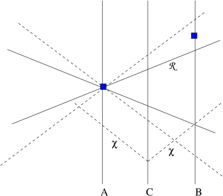
Figure 1: Oblivious embedding of protocol $\mathfrak{S}$ in a generic SRX characterized by $c<v_{\lambda}\leq\infty$. Alice’s, Bob’s and Charlie’s worldlines are the vertical lines labelled by $A,B$ and $C$, respectively. Alice’s and Bob’s measurement events $\textbf{e}_{A}$ and $\textbf{e}_{B}$ are indicated by the filled (blue online) square boxes. They are spacelike separated, but X-causally connected, with the X-cones indicated by the solid slanting lines. The lightcone is indicated by the dashed lines. The free will of Alice’s and Bob’s action is characterized by (20), where “past” is the past-half as seen in the PRF. Randomness $\chi$ and $\chi^{+}$ are pre-shared when the particles are distributed to Alice and Bob, while $\mathcal{R}$ is transmitted from Alice’s measurement event to Bob’s worldline with speed $v_{\lambda}$.

For any fixed SRX with $v_{\lambda}<\infty$, one can choose an experimental set-up such that Eq. (55) is violated, which would lead to a breakdown in quantum correlations. Not only that, such breakdowns could be used as a basis for superluminal signaling at the operational level through the violation of hidden influence inequalities Bancal et al. (2012); Barnea et al. (2013), as discussed below, implying that only the Newtonian SRX, characterized by $v_{\lambda}:=\infty$, is unconditionally valid.

VII.3 Hidden influence inequalities and the Newtonian SRX

In our framework, the validity of the extension requires condition the satisfaction of Ineq. (55). If it fails (e.g., because Alice and Bob measured almost simultaneously as seen in the PRF), then there is a breakdown in the nonlocal correlations, and the extension of QM produced by the embedding is invalid, even though the protocol $\mathfrak{S}$ is sound.

This breakdown would be experimentally testable (cf. Scarani et al. (2014) and references therein). But the main difficulty with the breakdown is that one can construct hidden influence inequalities Bancal et al. (2012); Barnea et al. (2013) which can exploit this breakdown to send superluminal signals at the operational level, in violation of Eq. (6) even when Alice and Bob make measurements freely.

The basic idea here may explained as follows Ryff . Alice and Bob share the state $\frac{1}{\sqrt{2}}(|0\rangle_{A}|00\rangle_{B}+|1\rangle_{A}|11\rangle_{B})$, in such a way that Bob’s two particles are spatially separated from each other by distance $R$, while at the same time they are equidistant from Alice’s particle at distance $L$, where $L\gg R$. Alice has the choice of measuring her particle at time $t_{A}$ in the computational basis or not measuring at all. Bob has pre-programmed his particles to be measured in the computational basis simultaneously at time $t_{B}$. Let $\infty>v_{\lambda}>\frac{L}{t_{B}-t_{A}}>c$. Bob’s two particles will fail condition (55) because in this case $v_{\rm exp}=\infty$. Therefore, his two particles will produce uncorrelated outcomes if Alice did not measure. But if she does measure, then $v_{\rm exp}=\frac{L}{t_{B}-t_{A}}$ and her influence satisfies (55), and therefore both of Bob’s particles will be set to the same value, producing correlated outcomes. Thus she can signal him superluminally if $v_{\lambda}$ is finite.

Therefore, the only SRX that can result in a valid extension is the Newtonian SRX, for which $\theta_{\lambda}=\frac{\pi}{2}$, guaranteeing the general satisfaction of Eq. (55). This can be shown to be true, even going beyond the above single-parameter family of SRXs. For example, consider the SRX obtained by replacing the universal PRF considered above by a PRF that is identified with the reference frame of Alice’s detector or Bob’s detector. This yields a valid extension provided Alice and Bob are agreed on the time-ordering of their respective detection events Suarez and Scarani (1997). But when the relative motion between the two detectors is such that the two reference frames disagree on the time-ordering of the two detection events, then a breakdown in the correlations is predicted at the operational level, which can be used as the basis for violating operational no-signaling assuming maximal free will Suarez (2013).

We conclude that given a sound simulation protocol, it leads to a valid extension if and only if the embedding is Newtonian. In practice, we can replace the infinite value of $v_{\lambda}$ by a sufficiently high speed so that $\mathcal{R}$ traverses the length of the universe (about $13\times 10^{10}$ Lyr) in unit time (say, Planck time, about $5\times 10^{-44}$ sec), which gives $v_{\lambda}>10^{61}c$ Garisto (2002). But this is a quantum gravity issue that we ignore here.

VIII Implications for ontological extensions

The embedding of $\mathfrak{S}$ directly demonstrates how to create an ontological extension for (the considered fragment of) QM. Thus, the simulation resources can now be re-interpreted as variables in the ontological extension, as per Eq. (4). Randomness $I_{R}$ and signaling $S_{R}$ can be replaced by the corresponding ontological quantities, namely indeterminism $I_{\lambda}$ and ontological signaling $S_{\lambda}$.

VIII.1 Complementarity in the ontological extension

For simulating a singlet, we require the resource given by a $C$-box with $C=1$. Substituting this in Eq. (49) yields

$$S_{R}+2I_{R}\geq 3F-2,$$ (56)

where $\frac{2}{3}\leq F\leq 1$. Setting $F=1$ in (56) gives Alice and Bob full free will in the sense analogous to that considered in Refs. Conway. and Kochen. (2006); *CK09; Colbeck and Renner (2011), and gives us Eq. (41) applied to simulation resources: $S_{R}+2I_{R}\geq 1$.

Under the identification (4), the complementarity (56) becomes the corresponding ontological complementarity: $S_{\lambda}+2I_{\lambda}\geq 3F-2$, where the reduced free will in the extension is implemented as described in Section B. We then have Eq. (5), which is repeated here:

$$S_{\lambda}+2I_{\lambda}\geq 1,$$ (57)

assuming full free will.

Result (57) can now be used as a basis to derive the Free Will Theorem Conway. and Kochen. (2006); *CK09 and the Unextendability Theorem Colbeck and Renner (2011) in the context of singlet statistics. From Eq. (57), it follows that

$$I_{\lambda}=0\implies S_{\lambda}>0,$$ (58)

which is an operational form of Bell’s theorem. Eq. (58) asserts that any deterministic model of singlet statistics must necessarily be signaling. In the context of singlet statistics, Eq. (58) is also the essential mathematical content of the Free Will Theorem Conway. and Kochen. (2006); *CK09, which assumes that $S_{\lambda}=0$ by appeal to SR, and thereby concludes that $I_{\lambda}>0$, i.e., “particles have free will”.

Further, from (57), we have the stronger result:

$$I_{\lambda}<\frac{1}{2}\implies S_{\lambda}>0,$$ (59)

which asserts that any predictively superior extension for the statistics of singlets will be signaling. In the context of singlet statistics, (59) is the essential mathematical content of the unextendability result Colbeck and Renner (2011). By appeal to SR and to the definition of free will (20) with scope of past given by $\overline{\mathcal{T}^{+}}$, Ref. Colbeck and Renner (2011) also requires that $S_{\lambda}=0$, and therefore, on basis of Eq. (59), excludes predictively superior ($I_{\lambda}<\frac{1}{2}$) extensions.

Despite this, our explicit construction of a non-covariant extension for QM showed that non-vanishing $S_{\lambda}$ is “harmless”, i.e., that does not violate operational no-signaling and does not undermine a suitably defined free will. In fact, it is necessary for constructing predictively superior extensions. In this light, it is clear that the requirement that extensions of QM should be non-signaling is unfavorable to extend QM. The fundamental assumption of Refs. Conway. and Kochen. (2006); *CK09; Colbeck and Renner (2011), that leads them to this requirement is that the causal structure of the spacetime of the extension also is Minkowskian. The non-covariance of an ontological extension for QM carries no physical consequence and thus bears no operational significance.

We note that the complementarity relation we obtained and the above conclusions drawn from it would apply also to any non-signaling operational theory, including one in which the CHSH-Bell inequality is violated up to the algebraic maximum. However, the question of why QM does not allow the violation of the CHSH-Bell inequality up to its algebraic maximum Popescu and Rohrlich (1994), an open problem in quantum foundations, is as such not addressed in our model.

VIII.2 Bohmian and GRW-type collapse models

Our above analysis of the randomness-signaling complementarity transferred to the obliviously embedded protocol provides a general clarification regarding why there is no bar against the compatibility between SR and predictively superior ontological extensions of QM. Bohmian mechanics Bohm (1952a); *Boh52b and GRW-like collapse models Ghirardi et al. (1986); Tumulka (2006a); *Tum06b provide specific instances where the non-covariant ontological elements are seen to reproduce a covariant operational theory (which is exactly QM in the case of Bohmian mechanics).

For ontological models derived by embedding simulation protocols in spacetime, our approach shows that predictively superior extensions of QM will contain elements in the ontological level that are necessarily non-covariant but “harmless”. If an ontological model is not manifestly reducible to a simulation protocol embedded in spacetime in the above fashion, then the operational/ontological level separation may not correspond to the covariant/noncovariant division of elements in the model. Indeed, for the GRW model Suarez (2010); Tumulka (2006a); *Tum06b; Bedingham et al. (2014) and Bohmian model Dürr et al. (2014), elements that are recognized as ontological in the respective model are given a covariant description. However, it is known that for any model of quantum nonlocality, there would be fundamental influences and fundamental correlations that lack a covariant description Hardy and Squires (1992); Gisin (2011); Aharonov and Albert (1984); Ghirardi (2000), and this idea receives a particularly clear and simple elucidation in our approach.

For example, in the case of the Bohmian mechanics, the information about the measurement-induced deformation of the quantum potential requires instantaneous signaling in a universal PRF Bohm and Hiley (1993), and may be identified with the ontological version of $\mathcal{R}$ with $S_{\lambda}>0$. The concept of obliviousness in the present context, then, is analogous to that of “absolute uncertainty” discussed in Ref. Dürr et al. (1992).

IX Discussions

We now briefly indicate other implications of our work. Our ontological model of QM derived from a simulation protocol provides a “behind the scenes” mechanism in the spirit of Bell Davies and Brown (1989) for explaining quantum correlations, which (again in Bell’s words) “cry out for explanation” (Bell, 1987, Ch.  9). Moreover, without the ontological extendability of SR, the experimental fact of quantum nonlocality would compel us to regard free will and no-signaling as logically dependent. We saw that in the Newtonian extension, free will can coexist with superluminal signaling. The concept of SRX thus frees us from this epistemological obligation.

QM and relativity theory form the corner-stones of modern physics. Yet, ironically, both have resisted unification. It is generally acknowledged that the reasons for this impasse are related to general relativity, and that quantum field theory evidences the harmonious unification of QM and SR. However, studies in the foundations of quantum nonlocality suggest that there is a “tension” between quantum nonlocality and SR in the sense, as seen above, that non-trivial extensions of QM will be signaling. Yet we saw that such extensions need not pose a threat either to free will or to operational no-signaling. On this strength, we are led to believe that the unification of QM with general relativity in quantum gravity may also profit from a similar exercise, namely to unify the theories by unifying suitable ontological extensions.

Supplemental notes

Appendix A Oblivious embedding of protocol $\mathfrak{S}$ in a generic SRX: Free-willed scenario

We consider the case where Alice and Bob have maximal free will, but the SRX is not necessarily Newtonian. Suppose Alice’s and Bob’s spacelike-separated measurement events are $\textbf{e}_{A}$ and $\textbf{e}_{B}$, respectively. As seen in the PRF, let the spacetime coordinates of these two events be $(\textbf{x}_{A},t_{A})$ and $(\textbf{x}_{B},t_{B})$. Further, let $W$ denote the worldline along which their respective particles were received from a quantum source (the dashed lines labelled $\chi$ in Figure 1). We define the oblivious embedding of simulation protocol $\mathfrak{S}(\chi,\mathcal{R})$ in an SRX $\theta_{\lambda}$ as follows (see Section VII.1 and Figure 1).

Pre-sharing $\chi$ and $\chi^{+}$

The resources $\chi$ and $\chi^{+}$ are pre-shared along spacetime path $W$.

Free will

Alice and Bob choose their inputs freely, according to definition (20), with the scope of the past being he past half in the PRF, and not the complement of the future lightcone. Thus the concept of free will is manifestly non-covariant.

Superluminal transmission of $\mathcal{R}$ at $v_{\lambda}$

Without loss of generality, let $t_{A}<t_{B}$ in the PRF. It is assumed that the two events are X-causally connected, so that

$$\frac{1}{c}\frac{|\textbf{x}_{A}-\textbf{x}_{B}|}{|t_{A}-t_{B}|}\leq\tan\left(\theta_{\rm DI}\right),$$ (60)

and information about Alice’s input reaches Bob’s station in time for his measurement at $\textbf{e}_{B}$ as seen in the PRF. Condition (60) also is manifestly non-covariant. (The case where Eq. (60) fails is considered below in Section VII.3). Together with $\chi$ and $\chi^{+}$, this suffices for his station to compute his outcome $y$, consistent with the predictions of QM, by assumption of soundness of the protocol.

Obliviousness of $\chi,\chi^{+},\mathcal{R}$

Bob can only access the final outcome $y$ directly, but never $\chi,\chi^{+}$ and $\mathcal{R}$, except as he may infer by knowing $y$.

Under the embedding, the simulation resources $\chi,\chi^{+},\mathcal{R}$ take on an ontological significance in the extension so defined. The extension is Lorentz non-covariant, since $\mathcal{R}$ and free will are not covariant, being defined with reference to a PRF. One might say that “there is no story in relativistic spacetime” of nonlocality (cf. Gisin (2011)). By contrast, spontaneity being an operational concept, the scope of the past in its definition, which is the complement of the causal future in SR, is covariant.

The non-covariant definition of free will protects free will from the threat potentially posed by the ontological superluminal signaling: at $\textbf{e}_{A}$, the conditions (7) forbid ontological signaling into the past half as seen in the PRF, whereas Alice’s signal is directed into the future half as seen in the PRF; at $\textbf{e}_{B}$, Bob transmits no signal anyway, and hence his action does not contradict (7) in the stated scope. The crucial difference between the present definition of free will and that in Ref. Colbeck and Renner (2011) is in the scope of the past.

Appendix B Oblivious embedding of protocol $\mathfrak{S}$ in a generic SRX: Reduced freewill scenario

Thus any given $\Lambda$ above 2 and up to 4 can be achieved by just reducing the free will (12) from the maximal value of $F=1$ to

$$F^{\prime} \equiv 1-\frac{1}{3}\left(\frac{\Lambda}{2}-1\right)=1-\frac{C_{\Lambda}}{3},$$ (61)

where $C_{\Lambda}\geq 0$.

Let $\textbf{P}_{\mathcal{L}}$ be the “0-bit protocol” obtained by uniformly mixing the local-deterministic boxes $\textbf{d}^{j_{0}}$. Denote by $\textbf{P}_{\mathcal{L}}^{\ast}(\Lambda)$ the new protocol to realize $\Lambda$, obtained via reduction of free will applied to $\textbf{P}_{\mathcal{L}}$. This requires that we choose $F{:=}F^{\prime}$. It can be shown that $\textbf{P}_{\mathcal{L}}^{\ast}(\Lambda)\in\mathfrak{F}^{P}$, as shown earlier.

A more intuitive and implementationally straightforward approach to Theorem 1, would be as follows. The enhanced $\mathcal{L}$ mode can be visualized as a probabilistic mixture of the bound mode $\mathcal{L}$ and free mode $\mathcal{F}$, with both modes being set at the observed level of violation $C_{\Lambda}$. Mode $\mathcal{L}$ (resp., $\mathcal{F}$) is played with probability $p_{\mathcal{L}}$ ($p_{\mathcal{F}}$), with $p_{\mathcal{F}}+p_{\mathcal{L}}=1$. The “average” free will (henceforth also denoted $F$) in this “mixed mode” will be

$$F = p_{\mathcal{F}}\cdot 1+p_{\mathcal{L}}\cdot F^{\prime},$$ (62)

$$= 1-\frac{C_{\Lambda}}{3}\left(1-p_{\mathcal{F}}\right),$$

using Eq. (61). It follows from Eq. (62) that if $C_{\Lambda}>0$, then

$$p_{\mathcal{F}}=1-\frac{3}{C_{\Lambda}}(1-F).$$ (63)

If $C_{\Lambda}=0$, then we set $F=1$ irrespective of $p_{\mathcal{F}}$ according to Eq. (62). Averaging over the communication costs in the two scenarios, we find

$$S_{R}+2I_{R} \geq p_{\mathcal{F}}C_{\Lambda},$$ (64)

and Eq. (49) then follows using Eq. (63).

Therefore, an implementation to simulate the violation of CHSH inequality at a given level $\Lambda$ would be by probabilistically mixing a protocol $\textbf{P}^{\ast}_{\mathcal{L}}(\Lambda)$ with $\textbf{P}_{\mathcal{F}}(\Lambda)$, which is a $\mathcal{F}$-mode protocol in $\mathfrak{F}^{P}$ that violates (1) to the level $\Lambda$. The required mixed mode protocol is given by

$$\textbf{P}_{\mathcal{LF}}^{\ast}(\Lambda)\equiv p_{\mathcal{L}}\textbf{P}^{\ast}_{\mathcal{L}}(\Lambda)+p_{\mathcal{F}}\textbf{P}_{\mathcal{F}}(\Lambda).$$ (65)

Let $\chi^{\ast}$ be a bit string that encodes instructions on realizing $\textbf{P}_{\mathcal{LF}}^{\ast}(\Lambda)$. One way to use $\chi^{\ast}$ would be as follows: $\chi^{\ast}$ carries two bit strings $\chi^{\ast}_{1}$ and $\chi^{\ast}_{2}$: one executes $\textbf{P}^{\ast}_{\mathcal{L}}(\Lambda)$ when the $j$th bit of $\chi^{\ast}_{1}$ (denoted $\chi^{\ast}_{1}(j)$) is “0” and executes $\textbf{P}_{\mathcal{F}}(\Lambda)$ when $\chi^{\ast}_{j}(j)=1$. The bit string $\chi$ is used to realize the $\textbf{P}_{\mathcal{L}}$ and $\textbf{P}_{\mathcal{F}}$, while $\chi^{\ast}_{2}$ is used to boost $\textbf{P}_{\mathcal{L}}$ to $\textbf{P}_{\mathcal{L}}^{\ast}$.

The $C$-box defined by protocol $\textbf{P}_{\mathcal{LF}}^{\ast}(\Lambda)$ in Eq. (65) can be used as a subroutine to simulate a singlet, which would require mixing $\textbf{P}^{\ast}_{\mathcal{L}}(\Lambda=4)$ and $\textbf{P}_{\mathcal{F}}(\Lambda=4)$ protocols. Then $\textbf{P}_{\mathcal{LF}}^{\ast}(\Lambda)$ will in general be an “biased PR box” Aravinda and Srikanth (2015a), i.e., one that attains $\Lambda=+4$ but may be signaling (Section V.5). . We denote this $\chi^{\ast}$ enhanced protocol for simulating singlet statistics by $\mathfrak{S}(\chi,\chi^{+},\chi^{\ast},\mathcal{R})$. In such a protocol, although there is reduction in free will, there will be no reduction in spontaneity, which is a reasonable requirement.

Embedding protocol $\mathfrak{S}$ with reduced free will is similar to the above situation with maximal free will, except that additionally it requires pre-sharing or superluminal transmission of bit strings $\chi^{\ast}$ and (as explained below) $\mathcal{R}^{\ast}$. These additional resources must also be embedded obliviously. We shall consider two situations.

The first one involves embedding protocol $\mathfrak{S}(\chi,\chi^{+},\chi^{\ast},\mathcal{R})$ to realize $\textbf{P}_{\mathcal{LF}}^{\ast}(\Lambda{:=}4)$, i.e., one in which free will can be reduced by correlation between the underlying state and Alice’s and Bob’s choices. In this case, in addition to bit strings $\chi$ and $\chi^{+}$, the string $\chi^{\ast}$ is pre-shared in the same way, along worldline $W$. In one role, $\chi^{\ast}$ is used to choose between the free-willed and bound modes in the mixed mode picture to realize $\textbf{P}^{\ast}_{\mathcal{LF}}$. String $\chi$ is used to realize $\textbf{P}_{\mathcal{L}}$ and $\textbf{P}_{\mathcal{F}}$ individually, while $\chi^{\ast}$ in its second role is used to boost $\textbf{P}_{\mathcal{L}}$ to $\textbf{P}_{\mathcal{L}}^{\ast}$. This will realize a $C$-box with $C=1$. Finally this maximal $C$-box is consumed, along with $\chi^{+}$, to realize singlet statistics. The resulting correlations respect spontaneity (23), and consequently operational no-signaling (6).

In the second method, which also implements the scenario where Alice’s and Bob’s choices are spontaneous but lack free will, we shall allow Alice’s choice to influence Bob’s. We introduce $\mathcal{R}^{\ast}$, which is a secondary resource superluminally transmitted at speed $v_{\lambda}$ from Alice in the above embedding procedure. Among many ways to use this, a convenient one is to let $\mathcal{R}^{\ast}$ to function just like $\chi^{\ast}$. For example suppose the underlying state is $\lambda=\textbf{d}^{0_{0}}$. If Alice selects $a=0$ then $\mathcal{R}^{\ast}$ permits Bob to choose either input, but if $a=1$, then $\mathcal{R}^{\ast}$ instructs him to preferably choose $b=0$ in order to enhance the operationally observed $\Lambda$.

The comprehensive simulation protocol, available for embedding, will be denoted $\mathfrak{S}(\chi,\chi^{+},\chi^{\ast},\mathcal{R},\mathcal{R}^{\ast})$, which may generally involve using both $\chi^{\ast}$ and $\mathcal{R}^{\ast}$.