Abstract

We present a systematic exploration of dark energy and modified gravity models containing a single scalar field non-minimally coupled to the metric. Even though the parameter space is large, by exploiting an effective field theory (EFT) formulation and by imposing simple physical constraints such as stability conditions and (sub-)luminal propagation of perturbations, we arrive at a number of generic predictions. (1) The linear growth rate of matter density fluctuations is generally suppressed compared to $\Lambda$CDM at intermediate redshifts ($0.5\lesssim z\lesssim 1$), despite the introduction of an attractive long-range scalar force. This is due to the fact that, in self-accelerating models, the background gravitational coupling weakens at intermediate redshifts, over-compensating the effect of the attractive scalar force. (2) At higher redshifts, the opposite happens; we identify a period of super-growth when the linear growth rate is larger than that predicted by $\Lambda$CDM. (3) The gravitational slip parameter $\eta$—the ratio of the space part of the metric perturbation to the time part—is bounded from above. For Brans-Dicke-type theories $\eta$ is at most unity. For more general theories, $\eta$ can exceed unity at intermediate redshifts, but not more than about $1.5$ if, at the same time, the linear growth rate is to be compatible with current observational constraints. We caution against phenomenological parametrization of data that do not correspond to predictions from viable physical theories. We advocate the EFT approach as a way to constrain new physics from future large-scale-structure data.

1 Introduction

Understanding the nature of the present cosmic acceleration is an important and fascinating challenge. The standard paradigm—a cosmological constant $+$ Cold Dark Matter within the framework of general relativity ($\Lambda$CDM)—has so far held up remarkably well when tested against cosmological data [1, 2, 3, 4]. This is especially true for data on the background expansion history. Large scale structure data, in other words data that concern the fluctuations, are improving in precision—current constraints are broadly consistent with $\Lambda$CDM, although mild tensions exist (see e.g. [5, 6, 7, 8]). New surveys, such as DES [9], Euclid [10], DESI [11], LSST [12] and WFIRST [13], are expected to greatly tighten these constraints. An important question is whether or how these observations can be used to distinguish $\Lambda$CDM from other dark energy models [14, 15, 16, 17].

From the theoretical perspective, any form of dark energy that is not the cosmological constant would have fluctuations. These dark energy fluctuations can couple to matter or not. Or, in the frame where matter couples only to the metric (the frame we use in this paper), these dark energy fluctuations can kinetically mix with the metric fluctuations or not. Models that have no such mixing are quintessence models—they generally give predictions for structure growth fairly close to $\Lambda$CDM, especially if the background expansion history is chosen to match to the observed one, with the equation of state index close to $-1$. Models that have such mixing are modified gravity models, our primary interest in this paper.

Effective field theory provides a framework for systematically writing down the action that governs the dynamics of such dark energy fluctuations [18, 19, 20, 21, 22, 23, 24, 25, 26, 27] (see [28, 29, 30] for a numerical implementation of this formalism). The background cosmic expansion is treated as a given—matching that of the best-fit $\Lambda$CDM for instance—while the dark energy fluctuations are encoded by a single scalar, the Goldstone boson associated with spontaneously broken time-diffeomorphism in the gravity/dark energy sector. In this paper, we are interested in the linear evolution of fluctuations, thus we retain terms in the action up to quadratic order in a gradient expansion. An important feature of the effective field theory for dark energy is that the Ricci scalar comes with a general time-dependent coupling. This allows the accelerating background expansion to be driven by modified gravity effects, as opposed to what resembles vacuum energy.

At the level of linear perturbations, non-standard gravitational scenarios effectively result in a time- and scale-dependent modifications of the Newton’s constant $G_{\rm eff}$ and of the gravitational slip parameter $\eta$ [31]. The former quantity captures information about the way mass fluctuations interact in the universe, while the gravitational slip parameter quantifies any nonstandard relation between the Newtonian potential $\Phi$ (time-time part of the metric fluctuations) and the curvature potential $\Psi$ (space-space part).

Models of dark energy contain in principle so many parameters that it might seem hopeless to come up with robust, generic predictions for $G_{\rm eff}$, $\eta$. For example, Horndeski theory [32, 33]—the most general theory containing one additional scalar degree of freedom $\phi$, with second order equations of motion—depends on four arbitrary functions of $\phi$ and of the kinetic term $(\partial\phi)^{2}$. If we relax the condition of no-higher derivatives in the equations of motion to that of absence of pathological ghost instabilities, we end up with an even larger beyond Horndeski set of theories, dependent on six arbitrary functions of $\phi$ and $(\partial\phi)^{2}$ [34, 35].

One of the main purposes of this paper is to show that, despite such apparent freedom, the behavior of $G_{\rm eff}(z)$ and $\eta(z)$ as functions of the redshift has definite features common to all healthy dark energy models (models with no ghost and gradient instabilities, nor superluminal propagation) within the vast Horndeski class. As a corollary, we show that popular, phenomenological parameterizations of $G_{\rm eff}(z)$ and $\eta(z)$ do not capture their redshift-dependence in actual, physical models.

The phenomenology of theories containing up to two derivatives in the equations of motion has been explored in Ref. [24], hereafter paper I, where a complete separation between background and perturbations quantities has been obtained (see also [37]) and a systematic study of the growth index of matter density fluctuations has been initiated. As shown in paper I, the background evolution and the linear cosmological perturbations for any scalar-tensor theory of this type are entirely captured by one constant and five functions of time,

$$\left\{\Omega_{m}^{0},\ H(t),\ \mu(t),\ \mu_{2}(t),\ \mu_{3}(t),\ \epsilon_{4}(t)\right\}\,.$$ (1)

The above ingredients allow one to span the entire set of Horndeski theories, which can be seen as generalizations of galileon-theories [40]. Since also models of massive gravity [41] and bi-gravity [42] reduce to the galileons in the relevant (“decoupling”) limit [43, 44], aspects of these models are captured by our analysis. In the above, $\Omega_{m}^{0}=\rho_{m}(t_{0})/(3mp^{2}H_{0}^{2})$ is the present fractional energy density of non-relativistic matter; $H(t)$, the Hubble parameter, encapsulates the background expansion history; the $\mu$s are parameters of the perturbation sector with the dimension of mass, typically of order Hubble: $\mu(t)$ is the non-minimal coupling of Brans-Dicke (BD) theories, $\mu_{3}$ appears in cubic galileon- and Horndeski-3 (H3) theories, $\mu_{2}$ affects the sound speed of the scalar fluctuations, but has otherwise no bearing on the linear growth of matter fluctuations; $\epsilon_{4}$ is a dimensionless order one parameter present in galileon-Horndeski 4 and 5 (H45) Lagrangians. Note that the full Horndeski theory (H45) includes H3 which, in turn, includes BD. They all correspond to “sub-spaces” of different dimensionality in the space of theories, schematically shown in the following figure.

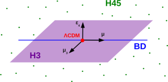
Figure 1: Pictorial representation of the space of theories spanned by the EFT coordinates $\mu,\mu_{3}$ and $\epsilon_{4}$.

The outline of the paper is as follows. We give an overview of the effective field theory formulation in Sec. 2, focusing on the quasi-static, sub-Hubble (or Newtonian) limit. We then work out the expressions for the gravitational coupling(s) and the gravitational slip parameter. We further reduce the degrees of freedom of the formalism by implementing viability conditions and by fixing the background expansion history (we choose the $\Lambda$CDM model which best fits the Planck’s satellite data [2]). In Sec. 3, we introduce the parametrization of the requisite time-dependent functions, and systematically scan the parameter space of general dark energy theories. We highlight the generic and robust predictions for the relevant large-scale-structure observables, such as the linear growth rate or the gravitational slip parameter. We conclude in Sec. 4 with a summary of the main results, and qualitative explanations for them.

2 Effects of dark energy on cosmological perturbations

There is a range of scales on which extracting perturbation observables from modified gravity (MG) theories is relatively straightforward: the window of comoving Fourier modes $k_{\rm sh}<k<k_{\rm nl}$. For momenta less than the non-linear scale, $k_{\rm nl}\simeq(10\,{\rm Mpc})^{-1}$, one can trust linear perturbation theory. For momenta well above the sound horizon scale $k_{\rm sh}\simeq aH/c_{s}$ ($c_{s}$ is the speed of sound of dark energy fluctuations), one can neglect the time derivatives of the metric and scalar fluctuations in the linear equations, the so called quasi-static approximation [56, 57]. In the quasi-static regime, it is possible to compute algebraically the effective Newton constant $G_{\rm eff}(t,k)$ and the gravitational slip parameter $\eta(t,k)$ of a given MG theory. The entire set of perturbation equations then reduces to

$$-\frac{k^{2}}{a^{2}}\Phi =4\pi G_{\rm eff}(t,k)\delta\rho_{m}\,,$$ (2)

$$\eta(t,k) =\frac{\Psi}{\Phi},\,$$ (3)

where we have adopted the following convention for the perturbed metric in Newtonian gauge,

$$ds^{2}=-(1+2\Phi)dt^{2}+a^{2}(1-2\Psi)\delta_{ij}dx^{i}dx^{j}\,.$$ (4)

Eqs. (2) and (3) should be supplemented by the equations for the matter fluctuation $\delta\rho_{m}$. Note that we work in the “Jordan frame”—one where all matter fields are minimally coupled to the metric (see [27] for a relaxation of this assumption within the effective field theory formalism) and do not couple directly to the dark energy fluctuation. This is the frame of most direct physical interpretation [53], where bodies follow geodesics.

In the rest of this section, we derive $G_{\rm eff}$ and $\eta$ in the framework of the effective field theory of dark energy (EFT of DE). We also clarify the relation between $G_{\rm eff}$ and the Newton constant $G_{N}$ measured, for example, in Cavendish experiments. Finally, we summarize the viability conditions to be imposed on our parameter space.

2.1 Gravitational couplings and gravitational slip

The linear cosmological perturbations of the class of theories considered in this paper are described by the unitary gauge action given in App. A. By moving to the more practical Newtonian gauge, we reintroduce the perturbation $\pi$ of the scalar field (dark energy fluctuation), along with the Newtonian potentials $\Phi$ and $\Psi$ defined in (4). The action quadratic in these quantities is very involved, but can be considerably simplified by the following approximations. First, we apply the quasi-static approximation, and neglect the time derivatives in the gravity-scalar sector. Second, in surveys of large scale structure, we generally observe modes well inside the Hubble horizon. We thus ignore mass terms in the perturbation quantities $\pi$, $\Phi$ and $\Psi$, because they are naturally of order Hubble and are small compared to the gradient terms—we retain the lowest gradients in the spirit of a gradient expansion. In this limit, all the dark energy models containing up to one scalar degree of freedom, and whose equations of motion have no more than two derivatives, are described by [35]

$$S=\int a\,M^{2} \left[(\vec{\nabla}\Psi)^{2}-2(1+\epsilon_{4})\vec{\nabla}\Phi\vec{\nabla}\Psi-2(\mu+\mathring{\epsilon}_{4})\vec{\nabla}\Psi\vec{\nabla}\pi\right.$$ (5)

$$\left.+\,(\mu-\mu_{3})\vec{\nabla}\Phi\vec{\nabla}\pi-\left({\cal C}+\frac{\mathring{\mu}_{3}}{2}-\dot{H}\epsilon_{4}+H\mathring{\epsilon}_{4}\right)(\vec{\nabla}\pi)^{2}\right]-a^{3}\,\Phi\delta\rho_{m},$$

where $\delta\rho_{m}$ is the perturbation of the non-relativistic energy density, a dot means derivative w.r.t. proper time and $\pi$ represents the perturbation of the scalar field. The non-minimal coupling $\mu$ and the “bare Planck mass” $M$ are related by

$$\mu\equiv\frac{d\ln M^{2}(t)}{dt},$$ (6)

and the expression of $\cal C$ is given as

$$\mathcal{C}\ =\ \frac{1}{2}(H\mu-\dot{\mu}-\mu^{2})-\dot{H}-\frac{\rho_{m}}{2M^{2}}\;.$$ (7)

In the above, $\rho_{m}\propto a^{-3}$ is the background energy density of non-relativistic matter. In minimally coupled scalar field models, we can think of ${\cal C}$ as related to the kinetic energy density of the field, ${\cal C}\sim\dot{\phi}^{2}/M^{2}$. To simplify the notation, we have also defined with a circle some “generalized time derivatives”:

$$\mathring{\mu}_{3}\ \equiv\ \dot{\mu}_{3}+\mu\mu_{3}+H\mu_{3},$$ (8)

$$\mathring{\epsilon}_{4}\ \equiv\ \dot{\epsilon}_{4}+\mu\epsilon_{4}+H\epsilon_{4}\,.$$ (9)

Variation of (5) with respect to the curvature potential $\Psi$ produces the algebraic relation

$$\Psi=(1+\epsilon_{4})\Phi+(\mu+\mathring{\epsilon}_{4})\pi$$ (10)

that, once substituted back into the action, gives

$$S=\int a\,M^{2} \left\{-(1+\epsilon_{4})^{2}(\vec{\nabla}\Phi)^{2}+\left[\mu-\mu_{3}-2(\mu+\mathring{\epsilon}_{4})(1+\epsilon_{4})\right]\vec{\nabla}\Phi\vec{\nabla}\pi\right.$$ (11)

$$\left.-\left[{\cal C}+(\mu+\mathring{\epsilon}_{4})^{2}+\frac{\mathring{\mu}_{3}}{2}-\dot{H}\epsilon_{4}+H\mathring{\epsilon}_{4}\right](\vec{\nabla}\pi)^{2}\right\}-a^{3}\,\Phi\delta\rho_{m}.$$

We can solve the coupled $\pi$-$\Phi$ system by taking the variation with respect to $\pi$, giving

$$\left[2{\cal C}+2(\mu+\mathring{\epsilon}_{4})^{2}+\mathring{\mu}_{3}-2\dot{H}\epsilon_{4}+2H\mathring{\epsilon}_{4}\right]\pi\ =\ \left[\mu-\mu_{3}-2(\mu+\mathring{\epsilon}_{4})(1+\epsilon_{4})\right]\Phi\,.$$ (12)

We thus conclude that the Newtonian gravitational potential $\Phi$ satisfies the Poisson equation

$$-\frac{k^{2}}{a^{2}}\Phi=4\pi G_{\rm eff}(t)\rho_{m}\delta_{m}\,,$$ (13)

where

$$G_{\rm eff}\ =\ \frac{1}{8\pi M^{2}(1+\epsilon_{4})^{2}}\ \frac{2{\mathcal{C}}+\mathring{\mu}_{3}-2\dot{H}\epsilon_{4}+2H\mathring{\epsilon}_{4}+2(\mu+\mathring{\epsilon}_{4})^{2}\ }{\ 2{\mathcal{C}}+\mathring{\mu}_{3}-2\dot{H}\epsilon_{4}+2H\mathring{\epsilon}_{4}+2\dfrac{(\mu+\mathring{\epsilon}_{4})(\mu-\mu_{3})}{1+\epsilon_{4}}-\dfrac{(\mu-\mu_{3})^{2}}{2(1+\epsilon_{4})^{2}}}\ .$$ (14)

As noted, we are neglecting any possible scale-dependence of $G_{\rm eff}$. The $k$-dependent corrections to (14) become important at large distances, how large depending on the size of the mass terms that we have neglected in (40). If the scalar degree of freedom, as we are assuming, plays a relevant role in the acceleration of the Universe, its mass is expected to be of order $H_{0}$ or lighter. Only Fourier modes approaching the Hubble scale are affected by such mass terms.

We need now to specify the relation between the effective Newton constant $G_{\rm eff}$ and the standard Newton constant $G_{N}$—or, equivalently, the Planck mass $M_{\rm Pl}$. Powerful Solar System [60, 61] and astrophysical [62, 63] tests impose stringent limits on modified gravity. Realistic models must incorporate “screening” mechanisms that ensure convergence to General Relativity on small scales and/or high-density environments. Horndeski theories mainly rely on the Vainshtein mechanism, which is now quite well understood also in a cosmological time dependent setup [48, 49, 50, 51]. In the vicinity of a massive body, the gravitational contribution of the scalar field fluctuation $\pi$ is suppressed because non-linear scalar self-interaction terms locally change the normalisation of the $\dot{\pi}^{2}$ term in the quadratic action [45]. This is equivalent to switching off the couplings of the canonically normalized $\pi$ to the other fields $\Psi$ and $\Phi$. Such an astrophysical effect cannot be encoded in our quadratic action (5), whose couplings depend only on time and not on space. However, by inspection of action (11) we conclude that in a screened environment, the “bare” gravitational coupling $M^{-2}$ gets simply dressed by a factor of $(1+\epsilon_{4})^{-2}$. This is what we obtain in the Poisson equation if we switch off the mixing term $\vec{\nabla}\Phi\vec{\nabla}\pi$. We thus define a screened gravitational coupling

$$G_{\rm sc}(t)\ \equiv\ \frac{1}{8\pi M^{2}(1+\epsilon_{4})^{2}}\,,$$ (15)

valid only in (totally) screened environments.

Since we live and perform experiments in a screened environment, the value of $G_{\rm cs}$ evaluated today is the Newton constant measured for example by Cavendish experiments,

$$G_{N}\ \equiv\ \frac{1}{8\pi M_{\rm Pl}^{2}}\ \simeq\ \frac{1}{8\pi M^{2}(t_{0})[1+\epsilon_{4}(t_{0})]^{2}}\,.$$ (16)

To complete the discussion, we would like to mention that the coupling of gravitational waves to matter contains, instead, only one factor of $(1+\epsilon_{4})$ at the denominator, and not two as $G_{\rm sc}$ [21, 35]. In ref. [37], the corresponding mass scale has been associated with the “Planck mass”. On the basis of the above arguments, here we find it more natural to define $M_{\rm Pl}$ as in (16) instead.

In summary, beyond the “bare” mass $M$ multiplying the Einstein Hilbert term in the unitary gauge action (40), we can define three gravitational couplings:

• $G_{\rm gw}\equiv\frac{1}{8\pi M^{2}(1+\epsilon_{4})}$ is the coupling of gravity waves to matter.

• $G_{\rm eff}$ given in eq. (14) is the gravitational coupling of two objects in the quasi-static approximation and in the linear regime, i.e. when screening is not effective. This is the quantity which is relevant on large (linear) cosmological scales.

• $G_{\rm sc}\equiv\frac{1}{8\pi M^{2}(1+\epsilon_{4})^{2}}$ is the gravitational coupling of two objects in the quasi-static approximation when screening is effective. Since the solar system is a screened environment, this is also the Newton constant measured by a Cavendish experiment, once evaluated at the present day: $G_{N}=G_{\rm sc}(t_{0})$.

Finally we note that even in the absence of anisotropic stress, the scalar and gravitational perturbations $\Phi$ and $\Psi$ are not anymore of equal amplitude, as predicted by general relativity. It is customary to describe deviations from the standard scenario by defining the gravitational slip parameter $\eta\ \equiv\ \frac{\Psi}{\Phi}$, which can be easily expressed within our formalism. By using (10) and (13) we obtain

$$\eta=1-\frac{(\mu+\mathring{\epsilon}_{4})(\mu+\mu_{3}+2\mathring{\epsilon}_{4})-\epsilon_{4}(2\mathcal{C}+\mathring{\mu}_{3}-2\dot{H}\epsilon_{4}+2H\mathring{\epsilon}_{4})}{2\mathcal{C}+\mathring{\mu}_{3}-2\dot{H}\epsilon_{4}+2H\mathring{\epsilon}_{4}+2(\mu+\mathring{\epsilon}_{4})^{2}}\,.$$ (17)

As for $G_{\rm eff}$, we note that not all deviations of $\eta$ from 1 are screenable in the conventional sense. From eq. (10), we see that in the presence of a non-vanishing $\epsilon_{4}$, the Newtonian potentials $\Psi$ and $\Phi$ are detuned from each other, even in environments where the $\pi$ fluctuations are heavily suppressed, $\eta_{\rm sc}\simeq 1+\epsilon_{4}$.

The above dark energy observables, $G_{\rm eff}$ and $\eta$, depend on the six functions $H(t)$, $M(t)$, $\mathcal{C}(t)$, $\mu(t)$, $\mu_{3}(t)$ and $\epsilon_{4}(t)$, which are constrained by Eqs. (6) and (7). Note also that the coupling $\mu_{2}(t)$ does not appear explicitly in the observables, it only plays a role in the stability conditions and the speed of sound of dark energy, as we show in the following. Below, we discuss how to reduce the dimensionality of this functional space to three constant parameters and three functions.

2.2 Theoretical constraints: viability conditions

One would expect a theory such as the EFT of DE, which depends on five free functions of time, to be virtually unconstrained and therefore un-predictive. What we will show instead is that, one can indeed bound the time evolution history of the relevant DE quantities such as $G_{\rm eff}$ and $\eta$ defined above. The key is to demand that the DE theories be free of physical pathologies.

We demand that a healthy DE theory satisfies the following four conditions: it must not be affected by ghosts, or by gradient instabilities; the scalar as well as tensor perturbations must propagate at luminal or subluminal speeds [47]. In what follows we simply refer to all these criteria as the stability or viability conditions. These conditions must be satisfied at any time $t$ in the past, while we do not enforce their future validity. We collect here the algebraic relations that enforce these requirements, allowing us to bound the time dependent couplings. An in-depth derivation and discussion of these relations can be found in paper I.

$$A\ >\ 0\qquad\qquad\text{no-ghost condition},$$ (18)

$$B\ \geq\ 0\qquad\qquad\text{gradient-stability condition},$$ (19)

$$c_{s}^{2}\ =\ \frac{B}{A} \leqslant\ 1\qquad\qquad\text{scalar subluminarity condition},$$ (20)

$$c_{T}^{2}\ =\dfrac{1}{1+\epsilon_{4}} \leqslant\ 1\qquad\qquad\text{tensor subluminarity condition},$$ (21)

where we have defined

$$A\ =\ (\mathcal{C}+2\mu_{2}^{2})(1+\epsilon_{4})+\frac{3}{4}(\mu-\mu_{3})^{2}\,,$$ (22)

$$B\ =\ (\mathcal{C}+\frac{\mathring{\mu}_{3}}{2}-\dot{H}\epsilon_{4}+H\mathring{\epsilon}_{4})(1+\epsilon_{4})-(\mu-\mu_{3})\left(\frac{\mu-\mu_{3}}{4(1+\epsilon_{4})}-\mu-\mathring{\epsilon}_{4}\right)\,.$$ (23)

2.3 Observational constraints: background expansion history

Recent observations tightly constrain the homogeneous background expansion history of the universe – equivalently, its Hubble rate $H(z)$ as a function of the redshift – to that of a spatially flat $\Lambda$CDM model [1, 2, 4]. We thus assume

$$H^{2}(z)=H_{0}^{2}\left[x_{0}(1+z)^{3}+\left(1-x_{0}\right)(1+z)^{3(1+w_{\rm eff})}\right]\,.$$ (24)

The quantities $x_{0}$—the present fractional matter density of the background – and $w_{\rm eff}$—the effective equation of state parameter – are free parameters, though observations suggest $x_{0}$ and $w_{\rm eff}$ must be close to $0.3$ and $-1$ respectively. Since we are interested in the recent expansion history, we have neglected the contribution of radiation.

The fractional matter density of the background reference model calculated at any epoch, $x$, proves a useful time variable for late-time cosmology, smoothly interpolating between $x=1$, deep in the matter dominated era, and its present value $x_{0}\simeq 0.3$. Its expression as a function of the redshift is

$$x\ =\ \frac{x_{0}}{x_{0}+(1-x_{0})(1+z)^{3w_{\rm eff}}}\,.$$ (25)

Having specified the background geometry $H(z)$, let us now see how this influences the functions $M^{2}(t)$ and $\mathcal{C}(t)$ that are needed to compute $G_{\rm eff}$ (14) and $\eta$ (17). First of all, note that $M^{2}(t)$ is not an independent free function of the formalism but is related to the non-minimal coupling $\mu$. By inverting eq. (6) we obtain

$$M^{2}(t)\ =\ \frac{M_{\rm Pl}^{2}}{(1+\epsilon_{4}^{0})^{2}}\,\exp\left(\int_{t_{0}}^{t}dt^{\prime}\mu(t^{\prime})\right),$$ (26)

where the initial conditions have been set according to (16). In a similar way, the evolution equations for the background (see e.g. [19, 24]) result in the expression of $\cal C$ given in (7). There, $\rho_{m}$ represents the physical energy density of non-relativistic matter. By “physical” we mean the quantity appearing in the energy momentum tensor. It scales as $a^{-3}$ since we are in the Jordan frame and $p_{m}\simeq 0$. With this quantity, we can define the physical fractional energy density

$$\Omega_{m}^{0}\equiv\frac{\rho_{m}(t_{0})}{3M_{\rm Pl}^{2}H_{0}^{2}}\,.$$ (27)

In principle, one could try to measure $\rho_{m}(t_{0})$ by directly weighing the total amount of baryons and dark matter, for instance within a Hubble volume. It is worth emphasizing that, in theories of modified gravity, $\Omega_{m}^{0}$ needs not be the same as $x_{0}$. The latter is a purely geometrical quantity, a proxy for the behavior of $H(z)$. It proves useful to define, as in paper I ,

$$\kappa\ \equiv\ \frac{\Omega_{m}^{0}}{x_{0}}\,.$$ (28)

In conclusion, the behavior of $G_{\rm eff}$ and $\eta$ is completely specified once the three parameters $x_{0},\ w_{\rm eff}$, and $\kappa$, and the three functions, $\mu(t),\ \mu_{3}(t),\ \epsilon_{4}(t)$, are supplied. Effectively, these functions are coordinates in the parameter space of modified gravity theories.

3 General predictions

In this section we describe the redshift scaling of interesting cosmological observables such as the effective Newton constant $G_{\rm eff}$, the linear growth rate of large scale structure $f$ and the gravitational slip parameter $\eta$.

3.1 Methodology

Before presenting our results, let us summarize the framework within which our predictions are derived. First of all, we enforce that viable modified gravity models reproduce the $\Lambda$CDM background history of the universe. In other words, we choose as background $H(z)$ that of a flat $\Lambda$CDM universe with parameters set by Planck ($x_{0}=0.314$ and $w_{\rm eff}=-1$).

As for the perturbed sector of the theory, we make the following assumptions

• We adopt $x$ as a useful time variable interpolating between the matter dominated era ($x=1$) and today ($x=x_{0}\simeq 0.3$), and expand the coupling functions up to second order as follows:

  $$\mu\left(x\right)\ =\ H(1-x)\left[p^{(0)}_{1}+p^{(1)}_{1}\left(x-x_{0}\right)+p^{(2)}_{1}\left(x-x_{0}\right)^{2}\right]\,,$$ (29)

  $$\mu_{3}\left(x\right)\ =\ H(1-x)\left[p^{(0)}_{3}+p^{(1)}_{3}\left(x-x_{0}\right)+p^{(2)}_{3}\left(x-x_{0}\right)^{2}\right]\,,$$ (30)

  $$\epsilon_{4}\left(x\right)\ =\ \ \ (1-x)\,\left[p^{(0)}_{4}+p^{(1)}_{4}\left(x-x_{0}\right)+p^{(2)}_{4}\left(x-x_{0}\right)^{2}\right]\,.$$ (31)

  On the other hand, we set $\mu_{2}=0$ since this function’s only effect is that of lowering the speed of sound of dark energy (see eq. 20) and thus reducing the range of validity of the quasi static limit, an approximation used in the present analysis. Secondly, we want to recover standard cosmology at very early times. This is why the Taylor expansions are multiplied by an overall factor of $(1-x)$ which serves to switch off the couplings at early epochs. This ties the modification of gravity to the (recent) phenomenon of dark energy.

• In the same spirit, we demand that the function ${\cal C}$, appearing in $G_{\rm eff}$ and $\eta$, grows at early epochs less rapidly than $H^{2}$ i.e. ${\cal C}/H^{2}\rightarrow 0$ at high redshift. In the limit of an (uncoupled) quintessence field $\phi$, ${\cal C}$ is nothing else than the kinetic fraction of the energy density of the field, ${\cal C}\sim\dot{\phi}^{2}/M_{\rm Pl}^{2}$. We are thus requiring that dark energy be subdominant at high redshift, which is usually the case in explicit models [38]. By inspection of equation (7), we see that we need a cancellation between the last two terms on the RHS. By substituting $\rho_{m}=3M_{\rm Pl}^{2}\kappa xH^{2}$ and using (28), we see that this condition is equivalent to setting the value of $M^{2}$ at early times,

  $$M^{2}\ \underset{x\rightarrow 1}{\longrightarrow}\ \kappa M_{\rm Pl}^{2}\,.$$ (32)

  By using (26), this imposes a constraint on the Taylor coefficients of $\mu$:

  $$\ln\left[\kappa(1+\epsilon_{4}^{0})^{2}\right]=\frac{1-x_{0}}{6w_{\rm eff}}\left[2p^{(1)}_{1}+p^{(2)}_{1}\left(1-3x_{0}\right)\right]-\frac{\ln\left(x_{0}\right)}{3w_{\rm eff}}\left[p^{(0)}_{1}-x_{0}p^{(1)}_{1}+x_{0}^{2}p^{(2)}_{1}\right].$$ (33)

  As we point out in the rest of the paper, some of the general features that we find are indeed related with this requirement.

• All of our analysis is carried out by assuming $\kappa=1$, i.e., by requiring that the physical and the effective reduced matter densities coincide at the present time. This choice is somewhat suggested by observations. Direct observations of the mass-to-light ratio on large scales lead to a value of $\Omega_{m}^{0}$ (see e.g. [39]) that is compatible with the “geometrical quantity” (here called $x_{0}$) obtained by fitting cosmological distances.

• We explore the space of non-minimal couplings $\mu$, $\mu_{3}$ and $\epsilon_{4}$ that covers the entire set of Hordenski theories by randomly generating points in the 8-dimensional parameter space of coefficients $p_{n}^{(i)}$ (note that in the $\mu$-sector the three $p_{1}^{(i)}$ are related by eq. 33). We reject those points that do not pass the stability conditions (18)-(21) until we have produced $10^{4}$ viable models. Note that, when dealing with the full 8-dimensional volume of parameters, the chance of hitting a stable theory is much lower than $1\%$. Because we want the quasi-static approximation to have a large enough range of applicability, we also impose $c_{s}>0.1$, which allows us to cover the Fourier volume of the EUCLID mission [57]. We emphasize, however, that this is a very weak selection effect on our randomly generated models.

• There is no “natural unit” in the space of Taylor coefficients. Mostly, we randomly generate them in the interval $p_{n}^{(i)}\in[-2,2]$, so that the relevant observables such as $f\sigma_{8}$ (see Figure 4) span the interval of uncertainty of current data. We have checked the robustness of our findings by expanding the ranges for different coefficients, and by raising the order of the expansions. A sample of these checks is reproduced in Figure 3. Additional checks that we have done include modeling the EFT couplings as step functions of variable height and width at characteristic redshifts and using different parameterizations for the BD sector. In particular, the one used in paper I is illustrated in App. B.

3.2 Evolution of the effective Newton constant

As mentioned, the redshift dependence of the effective Newton constant appears to be rather constrained by the stability conditions. Indeed, Figure 2 shows that the effective Newton constants in our large class of theories have similar evolution pattern over time. The universal behavior of $G_{\rm eff}(x)$ is best captured by the following few features. First, all the curves display a negative derivative at $x=1$, which implies stronger gravitational attraction ($G_{\rm eff}\geq G_{N}$) at early epochs ($z>2$). This behavior was proved analytically in paper I for a restricted set of models in which the Taylor expansion (29)-(31) is retained only at zeroth order. By inspection, we see here that the effect is still there at any order in the expansion. The amplitude of such an initial bump in $G_{\rm eff}(x)$ varies, with a few models displaying also conspicuous departures from the standard model. Also the width of the time interval over which this early stronger gravity period extends is quite model dependent. We find that the bump can be somewhat leveled out by giving up the requirement that DE be subdominant at high redshift (eqs. 32 and 33).

Even more interesting is the fact that all the models consistently predict that the amplitude of the effective gravitational coupling is suppressed $G_{\rm eff}\leq G_{N}$ in the redshift range $0.5\lesssim z\lesssim 1$ before turning stronger, once again, at around the present epoch.

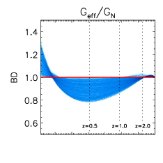
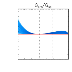
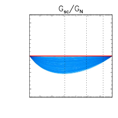
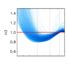
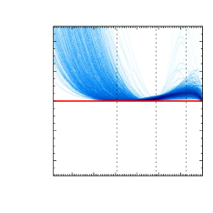
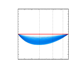
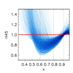
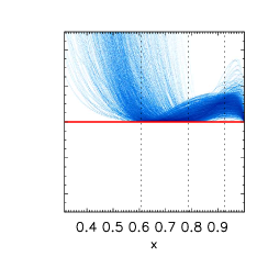
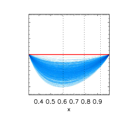
Figure 2: The behavior of $G_{\rm eff}$ (left panels) and its two separate contributions, from eq. (34) (central and right panels), as a function of the reduced matter density $x$ is shown for a sample of $10^{3}$ randomly generated models of viable BD, H3 and H45 theories. The dotted vertical lines identify, from left to right, the cosmic epochs $z=0.5$, $z=1$ and $z=2$. The thick red line represents $\Lambda$CDM. Note that H3 and H45 do not seem to approach this limit in a continuous way. The point is that BD, H3 and H45 correspond to “subspaces” of progressively higher dimensions in the theory space (see figure in Sec. 1). $\Lambda$CDM represents a well-defined limit for all models, but the volume of stable theories for H3 and H45 asymptotically reduces to an “hyperplane” of lower dimensions in the vicinity of $\Lambda$CDM. As a result, the neighborhood of $\Lambda$CDM is effectively a volume-zero subset for our random generator of theories. The Monte Carlo procedure does recover $\Lambda$CDM as a limiting case of BD nonetheless.

The reason for the intermediate range suppression is that at those redshifts the dominant contribution to the total of $G_{\rm eff}$ is given by the screened gravitational coupling $G_{\rm sc}$. Stability conditions always make $G_{\rm sc}$ lower than $G_{N}$ during the whole evolution. The characteristic S-shape pattern shown in Figure 2 is common to all models and does not depend on the degree of the Taylor expansion adopted for the coupling functions (29)-(31).

We should mention that, within covariant Galileon theories—a subclass of the models considered here—the same qualitative behavior of $G_{\rm eff}$ was found (see e.g. Ref. [58], Fig. 9, Ref. [59], Fig. 3), although the background evolution in that more constrained case is different from $\Lambda$CDM. Regarding the weaker gravitational attraction at intermediate redshifts, our results are in agreement with those of the recent paper [64]. Less clear to us is the role played by the gravitational wave speed $c_{T}$ (related to $\epsilon_{4}$, in our language) – the author of [64] claims $c_{T}<1$ is important for obtaining a weaker gravitational attraction. We find that a weaker gravitational attraction can be—and, in most cases, is—achieved also in theories (BD, H3) where $c_{T}=1$ (see also [65]).

A way to make sense of why the effective gravitational constant is stronger/weaker than the corresponding standard model value at characteristic cosmic epochs, is to decompose its amplitude into two distinctive parts. We can think of $G_{\rm eff}/G_{N}$ as the product of two terms,

$$\frac{G_{\rm eff}}{G_{N}}\ =\ \frac{G_{\rm eff}}{G_{\rm sc}}\ \frac{G_{\rm sc}}{G_{N}},$$ (34)

which can be expressed as (see eqs. 14 and 22)

$$\dfrac{G_{\rm eff}}{G_{\rm sc}}=1+\dfrac{1+\epsilon_{4}}{B}\left(\dfrac{\mu-\mu_{3}}{1+\epsilon_{4}}-(\mu+\mathring{\epsilon}_{4})\right)^{2}\,,\quad\qquad\dfrac{G_{\rm sc}}{G_{N}}=\dfrac{M_{\rm Pl}^{2}}{M^{2}(t)(1+\epsilon_{4})^{2}}\;,$$ (35)

respectively. Stability conditions (19) and (21) imply $G_{\rm eff}/G_{\rm sc}\geqslant 1$. Physically, this means that the scalar field contribution to the gravitational interaction is always attractive, as expected from a (healthy) spin-0 field. This circumstance is displayed in the second column of Figure 2.

The behavior of $G_{\rm sc}/G_{N}$, the last column of Fig. 2, also has a physical interpretation related to the stability of the models, although somewhat more subtle. First, note that the value of such a quantity today is unity by definition—as we have argued in (16), $G_{N}\equiv G_{\rm sc}(t_{0})$— while at early epochs ($x=1$) it is given by condition (32). On the other hand, the overall behavior of $G_{\rm sc}/G_{N}$ as a function of time can be understood as a product of the two independent factors, $M^{-2}$ and $(1+\epsilon_{4})^{-2}$. The latter quantity is always lower than unity because tensor perturbations are assumed to propagate at subliminal speed (see eq. 21). Also $M^{-2}$ decreases as a function of the redshift (i.e. backward in time) at around the present epoch. The physical reason is better understood in the “Einstein frame”—the frame in which the metric is decoupled from the scalar—which for the background evolution simply reads $g_{\mu\nu}^{(E)}\sim M^{2}(t)g_{\mu\nu}$ (see e.g. [19]). A growth of $M$ as a function of the redshift means less acceleration in the Einstein-frame, thus implying that the observed acceleration in the physical (Jordan) frame is due to a genuine modified gravity effect (self-acceleration). Therefore, the third column of Figure 2 provides a rough estimate of the amount of self-acceleration for the various randomly generated models. Curves that deviate the most from $\Lambda$CDM (the red straight line) represent models with strong self-acceleration, while the opposite cases represent models in which acceleration is essentially due to a negative pressure component in the energy momentum tensor. Our EFT approach covers both types of behavior in a continuous way, although it will be interesting to understand the specific features of those models that are truly self-accelerating [69].

3.3 The growth rate of matter fluctuations

The universal evolution of the effective Newton constant is expected to result in a characteristic growth history for the linear density fluctuations of matter. The prediction for this observable is obtained by solving the equation

$$3w_{\rm eff}(1-x)xf^{\prime}(x)+f(x)^{2}+\left[2-\frac{3}{2}\left(w_{\rm eff}(1-x)+1\right)\right]f(x)=\frac{3x}{2}\kappa\frac{G_{\rm eff}}{G_{N}}\,,$$ (36)

which approximates the true evolution in the Newtonian regime (below the Hubble scale) and well after the initial, radiation dominated phase of cosmic expansion. Here, $f\equiv d{\,\rm ln\,}\delta_{m}/d{\,\rm ln\,}a$, where $\delta_{m}$ is the matter fluctuation and $a$ is the scale factor.

Figure 3 shows that the expectation of a pattern of stronger/weaker growth phases with respect to the prediction of the standard model of cosmology is confirmed. Understandably, since $f$ obeys an evolution equation sourced effectively by $xG_{\rm eff}$, it responds to periods of stronger/weaker gravity with a time-lag. Moreover, as an integrated effect, $f$ has a smaller spread compared to $G_{\rm eff}$.

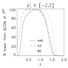
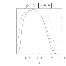
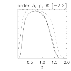
Figure 3: Percentage of randomly generated EFT models with growth rate $f$ lower than that predicted by $\Lambda$CDM Planck-cosmology as a function of the redshift $z$. We have checked the robustness of our analysis by changing the interval of the randomly generated Taylor coefficients (center) and by augmenting the order of the Taylor expansion (29)-(31) (right).

The first thing worth emphasizing is that essentially all modified gravity models with the same expansion history of $\Lambda$CDM consistently predict that cosmic structures grow at a stronger pace, compared to $\Lambda$CDM, at all redshifts greater than $z\sim 2$.

A second distinctive feature is that non-standard models of gravity are generally less effective in amplifying matter fluctuations during the intermediate epochs in which cosmic acceleration is observed, i.e. in the redshift range $0.5\lesssim z\lesssim 1$. Figure 3 shows that $95\%$ of the growth rates predicted in the BD, H3 and H45 classes of theories are weaker than expected in the standard $\Lambda$CDM scenario.

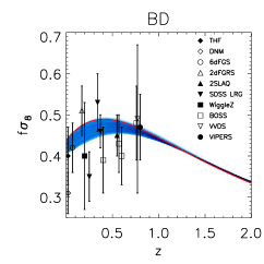
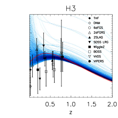
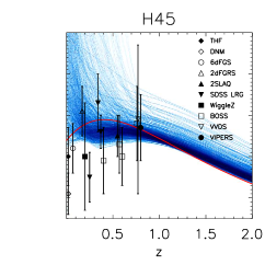
Figure 4: The redshift evolution of $f\sigma_{8}$ expected in $10^{3}$ stable EFT models is shown and compared to data. Error bars represent 1$\sigma$ s.d.. The evolution predicted by the best Planck fit is shown in red.

These predictions can be compared with observations. A collection of available measurements of the growth related quantity $f\sigma_{8}$ is presented in Figure 4 and compared to the most generic predictions of BD, H3 and H45 theories. The current errorbars are still large, thus one should not read too much into these plots. Nonetheless, it is intriguing that the data suggest less growth than is predicted by $\Lambda$CDM. If this holds up in future surveys, it would be important to check that growth is stronger than $\Lambda$CDM at $z>1$, as is predicted by the bulk of the models.

3.4 The gravitational slip parameter

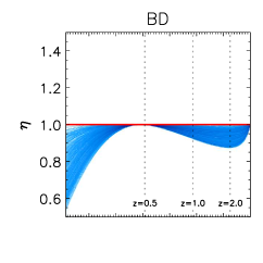
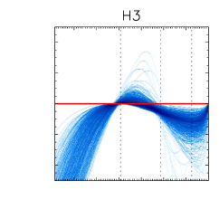
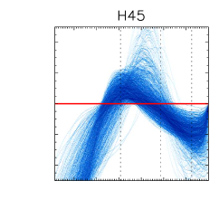
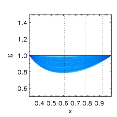
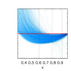
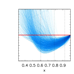
Figure 5: The amplitude of the gravitational slip $\eta$ and lensing potential $\Sigma$ as a function of the reduced matter density $x$ for $10^{3}$ EFT models. The expected values of both these functions in a $\Lambda$CDM cosmology are shown in red. The vertical dotted lines correspond from left to right to $z=0.5$, $z=1$ and $z=2$.

While the peculiar velocity of galaxies falling into the large scale overdensities of matter constrains the possible growth histories of cosmic structures, CMB and weak gravitational lensing provide complementary probe of gravity, notably they allow one to test whether the metric potentials $\Phi$ and $\Psi$ are indeed equal, as predicted by GR in the absence of anisotropic stress, or differ as predicted by most non-standard models of gravity.

Ref. [7] carried out an interesting joint analysis of current data using these three probes, obtaining constraints on two characteristic observables that are sensitive to non-standard behavior of the metric potentials. These are the gravitational slip parameter $\eta$, already introduced in Sec. 2.1, and the light deflection parameter or lensing potential $\Sigma$, defined in Fourier space by

$$-\frac{k^{2}}{a^{2}}\left(\Psi+\Phi\right)=8\pi\Sigma(t,k)\rho_{m}\delta_{m}\,,$$ (37)

which can be expressed as

$$\Sigma\ =\ \frac{G_{\rm eff}}{G_{N}}\,\frac{1+\eta}{2}\,.$$ (38)

For BD-like theories it is straightforward to show analytically that the amplitude of the curvature potential $\Psi$ is never greater than the Newtonian potential $\Phi$, that is, at any epoch, $\eta(t)\leq 1$. For this specific class of theories, the lensing potential reduces to $\Sigma=G_{\rm sc}/G_{N}$. From our earlier results (see Figure 2, right panels), we see that this observable cannot be larger than unity at any cosmic epoch, and must be equal to 1 (the $\Lambda$CDM value) at the present time.

When additional degrees of freedom are allowed (like in H3 and/or H45 models), we still find distintive features in the evolution of $\eta$ and $\Sigma$. Indeed, the slip parameter is always smaller than unity at any redshift except possibly in the window $0.5<z<1$, where relevant deviations from the $\Lambda$CDM expectations can be observed. Moreover, $\eta$ is never larger than $\sim 1.5$ at any cosmic epoch. Similar to the case of BD-like theories, the lensing potential $\Sigma$ is weaker than the standard model value at high redshifts ($z>0.5$–$1$), but becomes stronger (greater then unity) in recent epochs. Indeed, virtually all H3 and H45 models predict an amplitude of $\Sigma$ greater than 1 at the present time.

3.5 Comparison with ad-hoc phenomenological parameterizations

Given the lack of a compelling model to rival GR, it is common to parameterize deviations from GR in a phenomenological manner [31, 68, 7]. Previous works used simple monotonic time evolution for the relevant large-scale structure observable $O(t)$ (be it $G_{\rm eff}/G_{N}$, $\Sigma$ or $\eta$). For instance, the time evolution is often chosen to be proportional to the effective dark energy density implied by the background dynamics,

$$O(t)=1+O_{0}(1-x).$$ (39)

so that the modified gravity scenario converges to the standard picture at high redshifts. Note that such a simple ansatz corresponds to straight lines in our figures 2 and 5, a time dependence that does not seem to correspond to any viable single scalar field model. Instead, it appears from our analysis as if there is an additional time scale, roughly located between $z=0.5$ and $z=1$. All relevant quantities undergo a transition at that scale, typically reaching a local maximum ($\eta$) or a minimum ($G_{\rm eff}/G_{N}$ and $\Sigma$). This behavior is not captured by the “flat” parameterization (39).

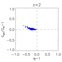
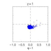
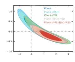
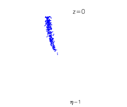
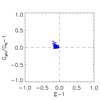
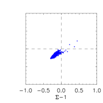
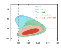
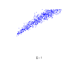
Figure 6: Left and central panels: Correlations between $G_{\rm eff}/G_{N}-1$ and $\eta-1$ (top line), $G_{\rm eff}/G_{N}-1$ and $\Sigma-1$ (bottom line) at redshifts 1 and 2 for $10^{4}$ stable H45 models. Right panel: The locus of points of the stable modified gravity theories encompassed by the EFT formalism is also shown at redshift equal to 0. The 2D likelihood constraints obtained by Planck [7] using a phenomenological parameterisation for the time evolution of $\Sigma$ and $\eta$ similar to that shown in eq. (39) is overplotted.

More interestingly, once the EFT formalism is fully and consistently applied, $G_{\rm eff}/G_{N}$ and $\eta$—as well as $G_{\rm eff}/G_{N}$ and $\Sigma$—appear not to be functionally independent quantities. A strong correlation exists among these pairs of observables which, in addition, evolves as a function of time. This correlation is displayed in Figure 6 at three different redshifts for the general class of H45 models. This is yet another instructive example of the general property already discussed in paper I, i.e. the requirement of physical stability significantly narrows the region of the parameter space. Despite the large number of degrees of freedom encompassed by the EFT formalism, model predictions are tightly confined within a limited region in the 2-dimensional planes $G_{\rm eff}/G_{N}-\eta$ and $G_{\rm eff}/G_{N}-\Sigma$ at a given redshift.

Existing constraints on $G_{\rm eff}/G_{N}$, $\Sigma$ and $\eta$ should be interpreted with care: they are sensitive to assumptions made concerning their time evolution. This is illustrated in the last panel of Figure 6. We superimpose the observational constraints on these variables set by Planck [7]—obtained by assuming the ansatz (39) for their time dependence—with the final (at $z=0$) values of the same quantities simulated with $10^{4}$ randomly generated viable theories. Fig. 6, interpreted at face-value, suggests viable EFT models—with their characteristic patterns shown in Figures 2 and 5—span a region of the parameter space that is mostly excluded by data. Such an interpretation is unwarranted. Suitable (non-monotonic) time-dependence of $G_{\rm eff}/G_{N}$, $\Sigma$ and $\eta$, in accordance with predictions from viable EFT models, must be included when performing the likelihood analysis [70].

4 Discussion and conclusions

We explore the phenomenological implications of a large class of dark energy models that result from adding a single scalar degree of freedom to the Einstein equations with equations of motion at most second order and allowing for non-minimal coupling with the metric. To do so, we exploit the effective field theory (EFT) of dark energy. It describes with a unifying language different, apparently unrelated, modified gravity theories, and allows us to directly connect these theories to observational signatures of departure from general relativity. By enforcing stability and (sub-)luminality constraints, we ensure whatever observational signatures that emerge are from theories free of physical pathologies.

In paper I the effective field theory of dark energy was used to predict the linear growth index of matter density perturbations. In this paper, we extend the formalism to compute a larger set of perturbation observables, including the effective Newton constant, the linear growth rate of density fluctuations, the lensing potential and the gravitational slip parameter. They are expressed in terms of the structural functions of the EFT formalism. Physical viability (i.e. freedom from pathologies) places strong constraints on these structural functions, greatly enhancing the predictive power of this approach.

In particular, the time dependence of $G_{\rm eff}(t)$ (the effective gravitational coupling in the Poisson equation 13), $f(t)$ (the growth function; eq. 36), and $\eta(t)$ (the slip parameter; eq. 17) for all Horndenski theories can be economically described in terms of three constant parameters ($x_{0},w_{\rm eff}$, and $\kappa$; eqs. 25, 28) which control the evolution of the background metric, as well as three functions ($\mu(t),\mu_{3}(t)$ and $\epsilon_{4}(t)$; eq. 5) which, being active in the perturbation sector, determine how matter fluctuations evolve in time at linear level. In this study we are interested in modified gravity models that are kinematically equivalent, i.e. share the same expansion history, but differ in their dynamical properties, i.e. predict different growth histories for large-scale structures. We thus factor out the background contributions to the amplitude of the large-scale structure observables by simply fixing the three constant parameters $x_{0},w_{\rm eff}$, and $\kappa$. We do this by requiring that the background expansion rate $H(t)$ be that of a $\Lambda$CDM model, notably the model that best fits Planck data [2]. The space of modified gravity theories is thus generated by the three non-minimal coupling functions $\mu(t)$, $\mu_{3}(t)$ and $\epsilon_{4}(t)$. To proceed further, we Taylor expand each EFT function, and scan the theory space by generating the expansion coefficients in a Monte Carlo fashion. An important point is that not all the models produced in this way are viable. There is a set of stability conditions that must be satisfied in order for a modified gravity theory to be healthy. These act as a severe selection on the parameter space and allow us to identify distinctive qualitative features of single scalar field dark energy models. We consider $10^{4}$ models surviving the stability criteria while matching the same cosmic expansion history.

This paper complements paper I in providing a maximal coverage of the viable theory space, and strengthening the robustness and generality of the predictions. We confirm two central findings of paper I, i.e. a) the space of theories naively allowed by cosmological data is much reduced once the viability criteria are applied; b) the vast majority of stable Horndeski theories produce an overall growth of structure at low redshifts that is weaker than that expected in a $\Lambda$CDM model. Here is a summary of our most important findings.

• Modified gravity does not necessarily imply stronger gravitational attraction. There are two effects that work in opposite directions. One effect is best seen in the Einstein frame—the frame where the metric is de-mixed from the scalar—the addition of an attractive scalar force indeed makes gravity stronger. This is equivalent to the statement that $G_{\rm eff}(t)>G_{\rm sc}(t)$ (see middle panels of Fig. 2). Note that this involves a ratio of the effective $G$ (that includes the effect of the scalar) and the “Einstein” $G$ (i.e. $G_{\rm sc}$) at the same time. A separate effect is encoded in the time-evolution of the bare Planck mass $M(t)$ (or of $G_{\rm sc}$). Models that achieve cosmic acceleration by virtue of a genuine modified gravity effect do so by giving $G_{\rm sc}$ a smaller value at intermediate redshifts ($z\sim 0.7$) than the current one, i.e. $G_{\rm sc}(t)<G_{\rm sc}(t_{0})$. When comparing structure growth in such models against that in general relativity, we are really asking the question: what is the ratio $G_{\rm eff}(t)/G_{\rm sc}(t_{0})$, since $G_{\rm sc}(t_{0})$ is the value of the gravitational coupling observed in the solar system today (we call this $G_{N}$). The ratio $G_{\rm eff}(t)/G_{\rm sc}(t_{0})$ can be written as $[G_{\rm eff}(t)/G_{\rm sc}(t)]\times[G_{\rm sc}(t)/G_{\rm sc}(t_{0})]$, hence it is a competition between two factors one larger, and one smaller, than unity. Indeed, we find that in a narrow redshift range around $z\simeq 0.7$ virtually all MG models display $G_{\rm eff}\leq G_{N}=G_{\rm sc}(t_{0})$. This feature is present also in the growth function $f$, though to a lesser degree because $f$ is an integrated quantity, dependent also on the behavior of $G_{\rm eff}$ at earlier cosmic times. In the redshift range $0.6\lesssim z\lesssim 0.8$, only $1\%(/5\%)$ of modified gravity models predict a value of $f(/f\sigma_{8})$ that is larger than the $\Lambda$CDM value. Recent observations suggest that the growth of structure in the low redshift universe is somewhat weaker than is expected in the best-fit $\Lambda$CDM model. It remains to be seen if this is confirmed by higher precision measurements in the future. It is nonetheless interesting that a weaker growth is predicted, at intermediate redshifts around $0.7$ or so, by the EFT of dark energy without fine tuning of the parameters.

• We identify an epoch of super-growth (i.e. faster growth than in $\Lambda$CDM) for cosmic structures. At sufficiently high redshifts, it is the first factor in $[G_{\rm eff}(t)/G_{\rm sc}(t)]\times[G_{\rm sc}(t)/G_{\rm sc}(t_{0})]$ that wins over the second factor. At high redshifts, there is no need for cosmic acceleration, thus $G_{\rm sc}(t)/G_{\rm sc}(t_{0})$ returns to unity, while $G_{\rm eff}(t)/G_{\rm sc}(t)$ remains larger than unity due to the presence of the scalar force. Indeed, as already demonstrated analytically in [24] for a more restricted number of models than is considered here, $dG_{\rm eff}(z)/dz$ is negative at the big-bang, implying a stronger gravitational attraction at high redshifts. More concretely, we find that for redshifts greater than $z=2$, both $f$ and $f\sigma_{8}$ are always larger than their $\Lambda$CDM values. This prediction could be used to potentially rule out the whole class of EFT models investigated in this paper. Structure growth at such high redshifts is poorly constrained by current data, but the situation will improve with future surveys such as Euclid, DESI or SKA.

• For Brans-Dicke theories, the gravitational slip parameter is at most one: $\eta\leqslant 1$. This can be shown analytically from Eq. (17), or qualitatively understood as follows. Absent anisotropic stress, $\Phi=\Psi$ in Einstein frame. The Jordan frame $\Phi$ and $\Psi$ are obtained from their Einstein frame counterparts by a conformal transformation involving the scalar $\pi$. Because $\Phi$ and $\Psi$ comes with opposite signs in the metric, the conformal transformation affects them differently, leading to $\eta-1\equiv(\Psi-\Phi)/\Phi\propto\pi/\Phi$, with a proportionality constant that makes $\eta-1\leqslant 0$ (recalling that $\pi\propto\Phi$ according to the equation of motion; see eq. 12). We find that this feature is substantially inherited by all theories, except for a narrow redshift range around $0.5\lesssim z\lesssim 1$ when $\eta$ exceeds one. For all theories we find $\eta<2$ at any redshift.

• The requirements of stability and (sub-)luminality help greatly in narrowing the viable parameter space of dark energy theories. Thus, despite the presence of several free functions in the EFT formalism, the class of theories we study is highly predictive. Moreover, the background expansion history is already well-constrained by current data, further limiting the form of the free functions. Applying the EFT formalism, we find interesting correlations between different large scale structure observables. In particular, at a given redshift, there exists only a narrow region in the 2-dimensional planes $G_{\rm eff}/G_{N}-\eta$ and $G_{\rm eff}/G_{N}-\Sigma$ where data can be meaningfully interpreted in terms of viable theories.

The systematic investigation by means of the EFT formalism of what lies beyond the standard gravity landscape is still in its infancy, and a number of improvements would be desirable. For example, it would be interesting to work out the consequences of relaxing some of the constraints imposed in our current analysis. How might our predictions be modified if a different initial condition were chosen ($\kappa\neq 1$), or if the background expansion history is altered ($w_{\rm eff}\neq-1$)? It would also be interesting to consider early dark energy models, in which a relevant fraction of dark energy density persists at early times (i.e. not imposing eqs. 32 and 33). We have focused on scales much smaller than the Hubble radius in this paper. As data improve on ever larger scales, our analysis should be extended to include possible scale dependent effects that come from mass terms for $\pi$ that are of the order of Hubble. Lastly, it would be useful to isolate models that have genuine self-acceleration, and compare their predictions with the ones studied here (which include both models that self-accelerate and models that do not).

Appendix A EFT action and relation with other equivalent parameterizations

While referring to the existing literature [19, 20, 21, 22, 23] for more details, here we just display the EFT action written in unitary gauge, which implicitly defines the couplings (1),

$$\begin{split}S\ =\ &\ S_{m}[g_{\mu\nu},\psi_{i}]\ \ +\int\!d^{4}x\sqrt{-g}\,\frac{M^{2}(t)}{2}\,\left[R\,-\,2\lambda(t)\,-\,2\mathcal{C}(t)g^{00}\,\right.\\ &\left.-\,\mu_{2}^{2}(t)(\delta g^{00})^{2}\,-\,\mu_{3}(t)\,\delta K\delta g^{00}+\,\epsilon_{4}(t)\left(\delta K^{\mu}_{\nu}\,\delta K^{\nu}_{\mu}-\delta K^{2}+\frac{\!\!{}^{(3)}\!R\,\delta g^{00}}{2}\right)\right]\;,\end{split}$$ (40)

Here the metric is the Jordan one, to which matter fields $\psi_{i}$ minimally couple (we are assuming the validity of the weak equivalence principle here, see [27] for a relaxation of this hypothesis). The functions $\lambda$ and ${\cal C}$ are constrained by the Friedman equations (see Sec. 2.3 or Ref. [24]).

In order to arrive at the action (5) from (40) we need to change gauge. The Stueckelberg procedure (see e.g. [23] for details) allows one to exit the unitary gauge by performing a time diffeomorphism $t\rightarrow t+\pi$, where $\pi$ represents the fluctuations of the scalar field, that now can appear explicitly in the action and in the equations. The Newtonian gauge then follows from further requiring a metric of the form (4). Note that the Stueckelberg procedure does not create direct coupling between $\pi$ and the matter fields, consistent with the fact that we are working in the Jordan frame, and the matter action is diff-invariant.

Finally, it is useful to write a dictionary relating our couplings to the equivalent “$\alpha$ couplings” defined in Ref. [37] (see also [26]):

$$\begin{split}M^{2}_{*}&=M^{2}\,(1+\epsilon_{4})\,,\\ \alpha_{M}&=\frac{\dot{\epsilon}_{4}}{H(1+\epsilon_{4})}+\frac{\mu}{H}\,,\\ \alpha_{K}&=\frac{2{\cal C}+4\mu_{2}^{2}}{H^{2}(1+\epsilon_{4})}\,,\\ \alpha_{B}&=\frac{\mu_{3}-\mu}{H(1+\epsilon_{4})}\,,\\ \alpha_{T}&=-\frac{\epsilon_{4}}{1+\epsilon_{4}}\;.\end{split}$$ (41)

Appendix B Exploring EFT models by means of a different parameterization scheme

In paper I a specific parametrization of the Brans-Dicke non-minimal coupling $\mu(t)$ was suggested, based on the “physical” equation of state parameter for dark energy $w\,=\,p_{D}/\rho_{D}\,$. This approach provides a complementary way to solve the background/perturbation sector degeneracy in the action (5) so that the function $\mathcal{C}$ is no longer free but is directly linked to $\mu$. The details about this parameterization scheme (the so called “$w$-parameterization” in opposition to the “$\mu$-parameterization” adopted in the current paper) can be found in Paper I. We briefly summarize here only the intermediate steps that are needed to relate these two parameterizations, and are thus important for expressing observable such as $G_{\rm eff}$ and $f\sigma_{8}$ in the language of paper I.

A little bit of algebra is enough to show that $\mu$ and the physical equation of state parameter $w$ are related as follows

$$\mu(x)=\dfrac{3w_{\rm eff}H(1-x)}{w-w_{\rm eff}(1-x)}\left[w-w_{\rm eff}+x(1-x)\frac{w_{\rm eff}}{w}\dfrac{dw}{dx}\right]\,.$$ (42)

One can thus proceed by expanding in Taylor series the function $w$ (instead of directly $\mu$, as we have done in this paper).

$$w\left(x\right)\ =\ w_{\rm eff}\,\dfrac{1-x_{0}}{1-\kappa\,x_{0}\,(1+\epsilon_{4}^{0})^{2}}+p^{(1)}_{1}\left(x-x_{0}\right)+p^{(2)}_{1}\left(x-x_{0}\right)^{2}\ ,$$ (43)

We should mention that the zero-th order term is fixed by requiring that the expansion rate of the various EFT models be identical to that of the reference flat $\Lambda$CDM scenario ( $w_{\rm eff}=-1$ and $x_{0}=0.314$). The other couplings functions are expanded as discussed in section 3.1 of the present paper. Figure 7 displays some of the results we obtain by implementing the $w$-parameterization scheme. Since there is no natural unit for the coupling functions, we chose to randomly pick $p_{1}^{(i)}\in[-0.8,0.8]$ (for $w$) and $p_{2,3}^{(i)}\in[-2,2]$ (for $\mu_{3}$ and $\epsilon_{4}$) in order for $f\sigma_{8}$ curves to cover current observational data as much as in the $\mu$-parameterization. The resemblance of $G_{\rm eff}/G_{N}$ to the one presented in Figure 2 confirms the robustness of our general findings; the universal behavior of $G_{\rm eff}$ (S-shape) is recovered no matter what parameterization is used for the coupling functions. In addition, the fraction of models with lower/higher growth with respect to $\Lambda$CDM displays the same general scaling as a function of $z$. We find that $\sim 90\%$ of H45 theories predict growth rates below the $\Lambda$CDM prediction in the redshift window $0.5\lesssim z\lesssim 1$. The change of parameterization implies a slight modification of the asymptotic behavior of the coupling functions $\mu$ and $\mathcal{C}/H^{2}$ at $x=1$, more precisely a modification of the speed at which these two functions go to zero during mater domination. This is well illustrated by the tail of the curves, the transition to the super-growth epoch is now shifted to a somewhat higher redshift ($z\sim 2.5$).

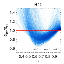
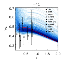
Figure 7: The plots displayed are computed in the $w$-parameterization scheme. The evolution of $G_{\rm eff}(x)$ (left), $f\sigma_{8}(z)$ (middle) for a sample of $10^{3}$ randomly generated models of viable H45 theories is shown. The percentage of $10^{4}$ randomly generated EFT models with growth rate $f$ lower than that predicted by $\Lambda$CDM Planck-cosmology as a function of the redshift $z$ (right) is also shown. The thick red line represents the prediction of $\Lambda$CDM.

References

- [1] M. Betoule et al. [SDSS Collaboration], “Improved cosmological constraints from a joint analysis of the SDSS-II and SNLS supernova samples,” Astron. Astrophys. 568, A22 (2014) [arXiv:1401.4064 [astro-ph.CO]].
- [2] P. A. R. Ade et al. [Planck Collaboration], “Planck 2015 results. XIII. Cosmological parameters,” arXiv:1502.01589 [astro-ph.CO].
- [3] J. Bel, C. Marinoni, B. R. Granett, L. Guzzo, J. A. Peacock, and E. Branchini et al., “The VIMOS Public Extragalactic Redshift Survey (VIPERS) : from the galaxy clustering ratio measured at ,” Astron. Astrophys. 563, A37 (2014) [arXiv:1310.3380 [astro-ph.CO]].
- [4] É. Aubourg, S. Bailey, J. E. Bautista, F. Beutler, V. Bhardwaj, D. Bizyaev, M. Blanton and M. Blomqvist et al., “Cosmological implications of baryon acoustic oscillation (BAO) measurements,” arXiv:1411.1074 [astro-ph.CO].
- [5] L. Samushia, et al., “The Clustering of Galaxies in the SDSS-III DR9 Baryon Oscillation Spectroscopic Survey: Testing Deviations from and General Relativity using anisotropic clustering of galaxies,” Mon. Not. Roy. Astron. Soc. 429, 1514 (2013) [arXiv:1206.5309 [astro-ph.CO]].
- [6] H. Steigerwald, J. Bel and C. Marinoni, “Probing non-standard gravity with the growth index: a background independent analysis,” JCAP 1405, 042 (2014) [arXiv:1403.0898 [astro-ph.CO]].
- [7] P. A. R. Ade et al. [Planck Collaboration], “Planck 2015 results. XIV. Dark energy and modified gravity,” arXiv:1502.01590 [astro-ph.CO].
- [8] P. A. R. Ade et al. [Planck Collaboration], “Planck 2015 results. XXIV. Cosmology from Sunyaev-Zeldovich cluster counts,” arXiv:1502.01597 [astro-ph.CO].
- [9] http://www.darkenergysurvey.org
- [10] http://www.euclid-ec.org
- [11] http://desi.lbl.gov/cdr/
- [12] http://www.lsst.org/lsst/
- [13] http://wfirst.gsfc.nasa.gov
- [14] S. Wang, L. Hui, M. May and Z. Haiman, “Is Modified Gravity Required by Observations? An Empirical Consistency Test of Dark Energy Models,” Phys. Rev. D 76, 063503 (2007) [arXiv:0705.0165 [astro-ph]].
- [15] L. Guzzo, M. Pierleoni, B. Meneux, E. Branchini, O. L. Fevre, C. Marinoni, B. Garilli and J. Blaizot et al., “A test of the nature of cosmic acceleration using galaxy redshift distortions,” Nature 451 (2008) 541 [arXiv:0802.1944 [astro-ph]].
- [16] L. Amendola, M. Kunz, and D. Sapone, ?Measuring the dark side (with weak lensing),? JCAP 4, 013 (2008), arXiv:0704.2421.
- [17] J. Bel, P. Brax, C. Marinoni and P. Valageas, “Cosmological tests of modified gravity: constraints on theories from the galaxy clustering ratio,” Phys. Rev. D 91, no. 10, 103503 (2015) [arXiv:1406.3347 [astro-ph.CO]].
- [18] P. Creminelli, G. D’Amico, J. Norena and F. Vernizzi, “The Effective Theory of Quintessence: the w¡-1 Side Unveiled,” JCAP 0902, 018 (2009) [arXiv:0811.0827 [astro-ph]].
- [19] G. Gubitosi, F. Piazza and F. Vernizzi, “The Effective Field Theory of Dark Energy,” JCAP 1302, 032 (2013) [arXiv:1210.0201 [hep-th]].
- [20] J. K. Bloomfield, E. Flanagan, M. Park and S. Watson, “Dark energy or modified gravity? An effective field theory approach,” JCAP 1308, 010 (2013) [arXiv:1211.7054 [astro-ph.CO]].
- [21] J. Gleyzes, D. Langlois, F. Piazza and F. Vernizzi, “Essential Building Blocks of Dark Energy,” JCAP 1308, 025 (2013) [arXiv:1304.4840 [hep-th]].
- [22] J. Bloomfield, “A Simplified Approach to General Scalar-Tensor Theories,” JCAP 1312, 044 (2013) [arXiv:1304.6712 [astro-ph.CO]].
- [23] F. Piazza and F. Vernizzi, “Effective Field Theory of Cosmological Perturbations,” Class. Quant. Grav. 30, 214007 (2013) [arXiv:1307.4350].
- [24] F. Piazza, H. Steigerwald and C. Marinoni, “Phenomenology of dark energy: exploring the space of theories with future redshift surveys,” JCAP 1405, 043 (2014) [arXiv:1312.6111 [astro-ph.CO]].
- [25] L. Á. Gergely and S. Tsujikawa, “Effective field theory of modified gravity with two scalar fields: dark energy and dark matter,” Phys. Rev. D 89, 064059 (2014) [arXiv:1402.0553 [hep-th]].
- [26] J. Gleyzes, D. Langlois and F. Vernizzi, “A unifying description of dark energy,” Int. J. Mod. Phys. D 23, no. 13, 1443010 (2015) [arXiv:1411.3712 [hep-th]].
- [27] J. Gleyzes, D. Langlois, M. Mancarella and F. Vernizzi, “Effective Theory of Interacting Dark Energy,” arXiv:1504.05481 [astro-ph.CO].
- [28] N. Frusciante, M. Raveri and A. Silvestri, “Effective Field Theory of Dark Energy: a Dynamical Analysis,” JCAP 1402, 026 (2014) [arXiv:1310.6026 [astro-ph.CO]].
- [29] B. Hu, M. Raveri, N. Frusciante and A. Silvestri, “Effective Field Theory of Cosmic Acceleration: an implementation in CAMB,” Phys. Rev. D 89, no. 10, 103530 (2014) [arXiv:1312.5742 [astro-ph.CO]].
- [30] M. Raveri, B. Hu, N. Frusciante and A. Silvestri, “Effective Field Theory of Cosmic Acceleration: constraining dark energy with CMB data,” Phys. Rev. D 90, no. 4, 043513 (2014) [arXiv:1405.1022 [astro-ph.CO]].
- [31] L. Pogosian, A. Silvestri, K. Koyama and G. B. Zhao, “How to optimally parametrize deviations from General Relativity in the evolution of cosmological perturbations?,” Phys. Rev. D 81, 104023 (2010) [arXiv:1002.2382 [astro-ph.CO]].
- [32] G. W. Horndeski, Int. J. Theor. Phys. 10, 363 (1974).
- [33] C. Deffayet, S. Deser and G. Esposito-Farese, “Generalized galileons: All scalar models whose curved background extensions maintain second-order field equations and stress-tensors,” Phys. Rev. D 80, 064015 (2009) [arXiv:0906.1967 [gr-qc]].
- [34] J. Gleyzes, D. Langlois, F. Piazza and F. Vernizzi, “Healthy theories beyond Horndeski,” arXiv:1404.6495 [hep-th].
- [35] J. Gleyzes, D. Langlois, F. Piazza and F. Vernizzi, “Exploring gravitational theories beyond Horndeski,” JCAP 1502, no. 02, 018 (2015) [arXiv:1408.1952 [astro-ph.CO]].
- [36] J. Wang, L. Hui and J. Khoury, “No-Go Theorems for Generalized Chameleon Field Theories,” Phys. Rev. Lett. 109, 241301 (2012) [arXiv:1208.4612 [astro-ph.CO]].
- [37] E. Bellini and I. Sawicki, “Maximal freedom at minimum cost: linear large-scale structure in general modifications of gravity,” JCAP 1407, 050 (2014) [arXiv:1404.3713 [astro-ph.CO]].
- [38] N. Chow and J. Khoury, “Galileon Cosmology,” Phys. Rev. D 80, 024037 (2009) [arXiv:0905.1325 [hep-th]].
- [39] N. A. Bahcall and A. Kulier, “Tracing mass and light in the Universe: where is the dark matter?,” Mon. Not. Roy. Astron. Soc. 439, no. 3, 2505 (2014) [arXiv:1310.0022 [astro-ph.CO]].
- [40] A. Nicolis, R. Rattazzi and E. Trincherini, “The galileon as a local modification of gravity,” Phys. Rev. D 79, 064036 (2009) [arXiv:0811.2197 [hep-th]].
- [41] C. de Rham and G. Gabadadze, “Generalization of the Fierz-Pauli Action,” Phys. Rev. D 82, 044020 (2010) [arXiv:1007.0443 [hep-th]].
- [42] S. F. Hassan and R. A. Rosen, “Confirmation of the Secondary Constraint and Absence of Ghost in Massive Gravity and Bimetric Gravity,” JHEP 1204, 123 (2012) [arXiv:1111.2070 [hep-th]].
- [43] C. de Rham, G. Gabadadze, L. Heisenberg and D. Pirtskhalava, “Cosmic Acceleration and the Helicity-0 Graviton,” Phys. Rev. D 83, 103516 (2011) [arXiv:1010.1780 [hep-th]].
- [44] M. Fasiello and A. J. Tolley, “Cosmological Stability Bound in Massive Gravity and Bigravity,” JCAP 1312, 002 (2013) [arXiv:1308.1647 [hep-th]].
- [45] E. Babichev and C. Deffayet, “An introduction to the Vainshtein mechanism,” Class. Quant. Grav. 30, 184001 (2013) [arXiv:1304.7240 [gr-qc]].
- [46] C. Deffayet, G. Esposito-Farese and A. Vikman, “Covariant galileon,” Phys. Rev. D 79, 084003 (2009) [arXiv:0901.1314 [hep-th]].
- [47] A. Adams, N. Arkani-Hamed, S. Dubovsky, A. Nicolis and R. Rattazzi, “Causality, analyticity and an IR obstruction to UV completion,” JHEP 0610, 014 (2006) [hep-th/0602178].
- [48] A. De Felice, R. Kase and S. Tsujikawa, “Vainshtein mechanism in second-order scalar-tensor theories,” Phys. Rev. D 85, 044059 (2012) [arXiv:1111.5090 [gr-qc]].
- [49] R. Kimura, T. Kobayashi and K. Yamamoto, “Vainshtein screening in a cosmological background in the most general second-order scalar-tensor theory,” Phys. Rev. D 85, 024023 (2012) [arXiv:1111.6749 [astro-ph.CO]].
- [50] K. Koyama, G. Niz and G. Tasinato, “Effective theory for the Vainshtein mechanism from the Horndeski action,” Phys. Rev. D 88, 021502 (2013) [arXiv:1305.0279 [hep-th]].
- [51] R. Kase and S. Tsujikawa, “Screening the fifth force in the Horndeski’s most general scalar-tensor theories,” JCAP 1308, 054 (2013) [arXiv:1306.6401 [gr-qc]].
- [52] C. Deffayet, X. Gao, D. A. Steer and G. Zahariade, “From k-essence to generalised Galileons,” Phys. Rev. D 84, 064039 (2011) [arXiv:1103.3260 [hep-th]].
- [53] F. Nitti and F. Piazza, “Scalar-tensor theories, trace anomalies and the QCD-frame,” Phys. Rev. D 86, 122002 (2012) [arXiv:1202.2105 [hep-th]].
- [54] L. Hui, A. Nicolis and C. Stubbs, “Equivalence Principle Implications of Modified Gravity Models,” Phys. Rev. D 80, 104002 (2009) [arXiv:0905.2966 [astro-ph.CO]].
- [55] R. Kase and S. Tsujikawa, “Cosmology in generalized Horndeski theories with second-order equations of motion,” arXiv:1407.0794 [hep-th].
- [56] J. Noller, F. von Braun-Bates and P. G. Ferreira, “Relativistic scalar fields and the quasistatic approximation in theories of modified gravity,” Phys. Rev. D 89, no. 2, 023521 (2014) [arXiv:1310.3266 [astro-ph.CO]].
- [57] I. Sawicki and E. Bellini, “Limits of Quasi-Static Approximation in Modified-Gravity Cosmologies,” arXiv:1503.06831 [astro-ph.CO].
- [58] J. Neveu, V. Ruhlmann-Kleider, A. Conley, N. Palanque-Delabrouille, P. Astier, J. Guy and E. Babichev, “Experimental constraints on the uncoupled Galileon model from SNLS3 data and other cosmological probes,” Astron. Astrophys. 555, A53 (2013) [arXiv:1302.2786 [gr-qc]].
- [59] A. Barreira, B. Li, C. Baugh, S. Pascoli, “Spherical collapse in Galileon gravity: fifth force solutions, halo mass function and halo bias”, JCAP 1311, 056 (2013) [arXiv:1308.3699 [astro-ph.CO]].
- [60] J. G. Williams, S. G. Turyshev and D. Boggs, “Lunar Laser Ranging Tests of the Equivalence Principle,” Class. Quant. Grav. 29, 184004 (2012) [arXiv:1203.2150 [gr-qc]].
- [61] B. Bertotti, L. Iess and P. Tortora, “A test of general relativity using radio links with the Cassini spacecraft,” Nature 425, 374 (2003).
- [62] B. Jain, V. Vikram and J. Sakstein, “Astrophysical Tests of Modified Gravity: Constraints from Distance Indicators in the Nearby Universe,” Astrophys. J. 779, 39 (2013) [arXiv:1204.6044 [astro-ph.CO]].
- [63] V. Vikram, A. Cabré, B. Jain and J. T. VanderPlas, “Astrophysical Tests of Modified Gravity: the Morphology and Kinematics of Dwarf Galaxies,” JCAP 1308, 020 (2013) [arXiv:1303.0295 [astro-ph.CO]].
- [64] S. Tsujikawa, “Possibility of realizing weak gravity in redshift-space distortion measurements,” arXiv:1505.02459 [astro-ph.CO].
- [65] V. Pettorino and C. Baccigalupi, “Coupled and Extended Quintessence: theoretical differences and structure formation,” Phys. Rev. D 77, 103003 (2008) [arXiv:0802.1086 [astro-ph]].
- [66] S. Dubovsky, T. Gregoire, A. Nicolis and R. Rattazzi, “Null energy condition and superluminal propagation,” JHEP 0603, 025 (2006) [hep-th/0512260].
- [67] P. Creminelli, M. A. Luty, A. Nicolis and L. Senatore, “Starting the Universe: Stable Violation of the Null Energy Condition and Non-standard Cosmologies,” JHEP 0612, 080 (2006) [hep-th/0606090].
- [68] F. simpson et al. ” CFHTLenS: testing the laws of gravity with tomographic weak lensing and redshift-space distortions” MNRAS —bf 429, 2249 (2013)
- [69] L. Hui, C. Marinoni, L. Perenon, F. Piazza, in preparation
- [70] C. Marinoni, F. Piazza and V. Salvatelli, in preparation.