Computational Extensive-Form Games

Abstract

We define solution concepts appropriate for computationally bounded players playing a fixed finite game. To do so, we need to define what it means for a computational game, which is a sequence of games that get larger in some appropriate sense, to represent a single finite underlying extensive-form game. Roughly speaking, we require all the games in the sequence to have essentially the same structure as the underlying game, except that two histories that are indistinguishable (i.e., in the same information set) in the underlying game may correspond to histories that are only computationally indistinguishable in the computational game. We define a computational version of both Nash equilibrium and sequential equilibrium for computational games, and show that every Nash (resp., sequential) equilibrium in the underlying game corresponds to a computational Nash (resp., sequential) equilibrium in the computational game. One advantage of our approach is that if a cryptographic protocol represents an abstract game, then we can analyze its strategic behavior in the abstract game, and thus separate the cryptographic analysis of the protocol from the strategic analysis.

1 Introduction

Game-theoretic models assume that the players are completely rational. This is typically interpreted as saying that payers act optimally given (their beliefs about) other players’ behavior. However, as was first pointed out by Simon [?], acting optimally may be hard. Thus, there has been a great deal of interest in capturing bounded rationality, and finding solution concepts appropriate for resource-bounded players.

One explanation of bounded rationality is that players have limits on their computational power. For example, the players might be able to use only strategies that can be implemented by a polynomial-time TM. While there has been a great deal of work [1, 4, 7, 6, 8, 9, 15] on solving game-theoretic problems using computationally bounded players, there has not really been a careful study of the solution concepts appropriate for such players. What does it mean, for example, to say that a fixed finite game played by polynomial-time players has a Nash equilibrium?

Consider for example the following two-player extensive-form game $G$: At the the empty history, player $1$ secretly chooses one of two alternatives and puts her choice inside a sealed envelope. Player $2$ then also chooses one of these two alternatives. Finally, player $1$ can either open the envelope and reveal her choice or destroy the envelope. If she opens the envelope and she chose a different alternative than player $2$, player 1 wins and gets a utility of 1; otherwise (i.e., if player 1 either chose the same alternative as player $2$ or she destroyed the envelope) player 1 loses and gets a utility of $-1$. Player’s 2’s utility is the opposite of player 1’s. The game tree for this game is given in Figure 1. Since player 2 acts without knowing 1’s choice, the two histories where 1 made different choices are in the same information set of player 2.

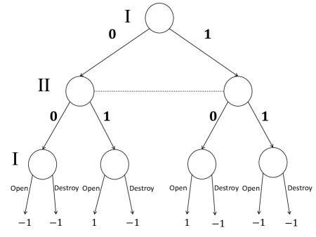
Figure 1: A game that can be represented by a computational game.

Resource-bounded players can implement this game even without access to envelopes, using what is called a commitment scheme. A commitment scheme is a two-phase two-party protocol involving a sender (player 1 above) and a receiver (player 2). The sender sends the receiver a message in the first phase that commits him to a bit without giving the receiver information about the bit (at least no information that he can efficiently compute from the message); this is the computational analogue of putting the bit in an envelope. In the second phase, the sender “opens the envelope” by sending the receiver some information that allows the receiver to confirm what bit the sender committed to in the first phase. Thus, we can talk about a game $\mathcal{G}$ (actually a sequence of games as discussed later) where instead of player 1 using an abstract envelope to send her choice to player 2, she uses a commitment scheme to do so.

Intuitively, we would like to say that the two games represent the same underlying game. However, there are many subtleties in doing so. To get a sense of the problems, note that to use commitment schemes we need the players to be computationally bounded. But to talk about computation bounds (for instance, polynomial-time TMs), we need to have a sequence of inputs that can grow as a function of $n$. So how do we proceed if we want to talk about computationally bounded players in a fixed finite game? The idea is that we will have a sequence of games, potentially increasing in size, that represents the single game. As we shall see, the information structure of the games in the infinite sequence might differ from that of the underlying game. For example, in the games described before, while a commitment scheme gives no information to a computationally bounded player, an unbounded player has complete information; the encrypted string uniquely identifies the bit that was committed. Thus, unlike in $G$, commitments to different bits in $\mathcal{G}$ are in different information sets for player $2$.

Additional complications arise when we consider solution concepts for such games. Traditional notions of equilibrium involve all players making a best response. But if we restrict to computationally bounded players, there may not be a best response, especially for the kinds of cryptographic problems that we would like to consider. For example, for every polynomial-time TM, there may be another TM that does a little better by spending a little longer trying to do decryption. (See [5] for an example of this phenomenon.) Moreover, when considering sequentially rational solution concepts it is unclear what information structure should be considered since, as we discussed, the information structure of the computational games does not capture the knowledge of computationally bounded players.

Our contributions.

As a first step to capturing these notions, in Section 3.1, we define what it means for a sequence $\mathcal{G}=(G_{1},G_{2},\ldots)$ of games to represent a single game $G$. Intuitively, all the games in the sequence $\mathcal{G}$ have the same basic structure as $G$, but might use increasingly longer strings to represent actions in $G$ (e.g., an action $a$ in $G$ might be represented in $G_{n}$ by an encryption of $a$ that uses a security parameter of length $n$). More precisely, we require a mapping from histories in the games $G_{n}$ to histories in $G$, as well as a mapping from strategies in $G$ to strategies in $\mathcal{G}$, and impose what we argue are reasonable conditions on these mappings. In Section 3.2, we show how this definition play out in the example discussed above.

As hinted before, our conditions do not force the games in $\mathcal{G}$ to have the same information structure as $G$. While two histories in the same information set in $G_{n}$ must map to two histories in the same information set in $G$, it may also be the case that two histories in different information sets in $G_{n}$ are mapped to the same information set in $G$. Although a player can distinguish two histories in different information sets (for example a commitment to $0$ and a commitment to $1$ in the example are two different strings), at a computational level, she cannot tell them apart. The encodings just look like random strings to her. There is a sense in which she, as a computationally bounded player, does not understand the “meaning” of these histories (although a computationally unbounded player could break the commitment and tell them apart). In Section 3.3, we make this intuition precise, showing that our requirements force all histories that map to the same information set in $G$ to be computationally indistinguishable, even if they are in different information sets in $\mathcal{G}$.

Once we have defined our model of computational games, we focus on defining analogues of two solution concepts, Nash equilibrium (NE) and sequential equilibrium. In Section 4.1, we define a computational analogues of NE, which considers only deviations that can be implemented by polynomial-time TMs. It handles previously mentioned complications by allowing for the strategy to be an $\epsilon$ best response for some negligible function $\epsilon$. (Our definition of NE is similar in spirit to the definition in Dodis, Halevi, and Rabin [?].) We show that if a strategy profile is a NE in the underlying game $G$, then there is a corresponding strategy profile of polynomial time TMs that is a computational NE in $\mathcal{G}$. Thus, we provide conditions that guarantee the existence of a computational NE, addressing an open question of Katz [?].

In Section 4.2, we define a computational analogue of sequential equilibrium. It is notoriously problematic to define sequentially rational solution concepts in cryptographic protocols. For example, Gradwohl, Livne, and Rosen [?] provide a general discussion of the issue, and give a partial solution in terms of avoiding what they call “empty threats”, which applies only to two-player games of perfect information, and discuss possible extensions. Our notion of computational sequential equilibrium, which is quite different in spirit from the solution concept of Gradwohl, Livne, and Rosen (and arguably conceptually much simpler and much closer in spirit to the standard game-theoretic definition), applies to arbitrary sequence of games that represent a finite game, and uses the intuitions we develop on the connection between information sets in the underlying finite game and computational indistinguishability in the sequence. We again show that if a strategy profile is a sequential equilibrium in the underlying game $G$, then there is a corresponding strategy profile of polynomial time TMs that is a computational sequential equilibrium in $\mathcal{G}$.

An important benefit of our approach is that it separates the game-theoretic analysis from the cryptographic analysis. We can view the sequence $\mathcal{G}$ as an implementation of an abstract game $G$. Given this view, we can first prove that a protocol is a good implementation of an abstract game, and then analyze the strategic aspects in that simple abstract game. For example, to show a prescribed cryptographic protocol is a Nash (resp., sequential) equilibrium, we can first show it represents an abstract ideal game; it then suffices to show that the protocol corresponds to a strategy profile that is a Nash (resp., sequential) equilibrium in the much simpler underlying game. We give an exmaple of this idea in Section 5, where we show how our approach can be used to analyze a protocol for implementing a correlated equilibrium (CE) without a mediator using cryptography, in the spirit of the work of Dodis, Halevy, and Rabin [?].

2 Preliminaries

2.1 Extensive-form games

We begin by reviewing the formal definition of an extensive-form game [12]. A finite extensive-form game $G$ is a tuple $([c],H,P,\vec{u},\vec{\mathcal{I}})$ satisfying the following conditions:

• $[c]=\{1,\ldots,c\}$ is the set of players in the game.

• $H$ is a set of history sequences that satisfies the following two properties:

  • the empty sequence $\langle\,\rangle$ is a member of $H$;

  • if $\langle a_{1},\ldots,a_{K}\rangle\in H$ and $L<K$ then $\langle a_{1},\ldots,a_{L}\rangle\in H$. The elements of a history $h$ are called actions.

  A history $\langle a_{1},\ldots,a^{K}\rangle\in H$ is terminal if there is no $a$ such that $\langle a^{1},\ldots,a^{K},a\rangle\in H$. The set of actions available after a nonterminal history $h$ is denoted $A(h)=\{a:h\cdot a)\in H\}$ (where $h\cdots a$ is the result of concatenating $a$ to the end of $h$. Let $H^{T}$ denote the set of terminal histories, let $H^{NT}$ denote $H\setminus H^{T}$, and let $H^{i}$ denote the histories after which player $i$ plays.

• $P:H\setminus H^{T}\to[c]$. $P(h)$ specifies the player that moves at history $h$.

• $\vec{u}:H_{T}\to\mathbb{R}^{c}$ specifies for each terminal history the utility of the players at that history ($u_{i}(h)$ is the utility of player $i$ at terminal history $h$).

• for each player $i\in[c]$, $\mathcal{I}_{i}$ is a partition of $H^{i}$ with the property that $A(h)=A(h^{\prime})$ whenever $h$ and $h^{\prime}$ are in the same member of the partition. For $I\in\mathcal{I}_{i}$, we denote by $A(I)$ the set $A(h)$ for $h\in I$ (recall that $A(h)=A(h^{\prime})$ if $h$ and $h^{\prime}$ are two histories in $I$). We assume without loss of generality that if $I\neq I^{\prime}$, then $A(I)$ and $A(I^{\prime})$ are disjoint (we can always rename actions to ensure that this is the case). We call $\mathcal{I}_{i}$ the information partition of player $i$; a set $I\in\mathcal{I}_{i}$ is an information set of player $i$; $\vec{\mathcal{I}}=(\mathcal{I}_{1},\ldots,\mathcal{I}_{c})$ is the information partition structure of the game. A game of perfect information is one where all the information sets are singletons.

This model can capture situations in which players forget what they knew earlier. Roughly speaking, a game has perfect recall if the information structure is such that the players remember everything they knew in the past.

Definition 2.1.

Let $\mathit{EXP}_{i}(h)$ be the record of player $i$’s experience in history $h$, that is, all the actions he plays and all the information sets he encounters in the history. A game has perfect recall if, for each player $i$, we have $\mathit{EXP}_{i}(h)=\mathit{EXP}_{i}(h^{\prime})$ whenever the histories $h$ and $h^{\prime}$ are in the same information set for player $i$.

A deterministic strategy $s$ for player $i$ is a function from $\mathcal{I}_{i}$ to actions, where for $I\in\mathcal{I}_{i}$, we require that $s(I)\in A(I)$. We also consider mixed strategies which are probability distribution over deterministic strategies. A profile of strategies $\vec{\sigma}=\{\sigma_{1},\ldots,\sigma_{c}\}$ induces a distribution denoted $\rho_{\vec{\sigma}}$ on terminal histories. We say that a strategy profile is completely mixed if $\rho_{\vec{\sigma}}$ assigns positive probability to every history $h\in H^{T}$. The expected value of player $i$ given $\vec{\sigma}$ is then $\sum_{h\in H^{T}}\rho_{\vec{\sigma}}(h)u_{i}(h)$.

We use the standard notation $\vec{x}_{-i}$ to denote the vector $\vec{x}$ with its $i$th element removed and $(x^{\prime},\vec{x}_{-i})$ to denote $\vec{x}$ with its $i$th element replaced by $x^{\prime}$.

Definition 2.2 (Nash Equilibrium).

$\vec{\sigma}=\{\sigma_{1},\ldots,\sigma_{c}\}$ is an $\epsilon$-Nash equilibrium (NE) of $G$ if, for all players $i\in[c]$ and for all strategies $\sigma^{\prime}$ for player $i$,

$$\sum_{h\in H^{T}}\rho_{\vec{\sigma}}(h)u_{i}(h)\geq\sum_{h\in H^{T}}\rho_{\sigma^{\prime},\vec{\sigma}_{-i}}(h)u_{i}(h)-\epsilon.$$

We now recall the notion of sequential equilibrium [11]. A sequential equilibrium is a pair $(\vec{\sigma},\mu)$ consisting of a strategy profile $\vec{\sigma}$ and a belief system $\mu$, where $\mu$ associates with each information set $I$ a probability $\mu(I)$ on the nodes in $I$. Intuitively, if $I$ is an information set for player $i$, $\mu(I)$ describes $i$’s beliefs about the likelihood of being in each of the nodes in $I$. Then $(\vec{\sigma},\mu)$ is a sequential equilibrium if, for each player $i$ and each information set $I$ for player $i$, $\sigma_{i}$ is a best response to $\vec{\sigma}_{-i}$ given $i$’s beliefs $\mu(I)$. An equivalent definition that does not require beliefs and is more suitable for our setting is given by the following theorem:

Theorem 2.3.

[11, Proposition 6] Let $G$ be an extensive-form game with perfect recall. There exists a belief system $\mu$ such that $(\vec{\sigma},\mu)$ is a sequential equilibrium of $G$ iff there exists a sequence of completely mixed strategy profiles $\vec{\sigma}^{1},\vec{\sigma}^{2},\ldots$ converging to $\vec{\sigma}$ and a sequence $\delta_{1},\delta_{2},\ldots$ of nonnegative real numbers converging to $0$ such that, for each player $i$ and each information set $I$ for player $i$, $\vec{\sigma}^{n}_{i}$ is a $\delta_{n}$-best response to $\vec{\sigma}^{n}_{-i}$ conditional on having reached $I$.

2.2 Computational indistinguishability

For a probabilistic algorithm $A$ and an infinite bitstring $r$, $A(x;r)$ denotes the output of $A$ running on input $x$ with randomness $r$; $A(x)$ denotes the distribution on outputs of $A$ induced by considering $A(x;r)$, where $r$ is chosen uniformly at random. A function $\epsilon:\mathbb{N}\rightarrow[0,1]$ is negligible if, for every constant $c\in\mathbb{N}$, $\epsilon(k)<k^{-c}$ for sufficiently large $k$.

Definition 2.4.

A probability ensemble is a sequence $X=\{X_{n}\}_{n\in\mathbb{N}}$ of probability distribution indexed by $\mathbb{N}$. (Typically, in an ensemble $X=\{X_{n}\}_{n\in\mathbb{N}}$, the support of $X_{n}$ consists of strings of length $n$.)

We now recall the definition of computational indistinguishability [3].

Definition 2.5.

Two probability ensembles $\{X_{n}\}_{n\in\mathbb{N}},\{Y_{n}\}_{n\in\mathbb{N}}$ are computationally indistinguishable if, for all PPT TMs $D$, there exists a negligible function $\epsilon$ such that, for all $n\in\mathbb{N}$,

$$|\Pr[D(1^{n},X_{n})=1]-\Pr[D(1^{n},Y_{n})=1]|\leq\epsilon(n).$$

To explain the $\Pr$ in the last line, recall that $X_{n}$ and $Y_{n}$ are probability distributions. Although we write $D(1^{n},X_{n})$, $D$ is a randomized algorithm, so what $D(1^{n},X_{n})$ returns depends on the outcome of random coin tosses. To be a little more formal, we should write $D(1^{n},X_{n},r)$, where $r$ is an infinitely long random bit strong (of which $D$ will only use a finite initial prefix). More formally, taking $\Pr_{X_{n}}$ to be the joint distribution over strings $(x,r)$, where $x$ is chosen according to $X_{n}$ and r is chosen according to the uniform distribution on bit-strings, we want

$$|{\Pr}_{X_{n}}\left[\{(x,r):D(1^{n},x,r)=1\}\right]-{\Pr}_{Y_{n}}\left[\{(y,r):D(1^{n},y,r)=1\}\right]|\leq\epsilon(n).$$

We similarly abuse notation elsewhere in writing $\Pr$.

We often call a TM $M$ that is supposed to distinguish between two probability ensembles a distinguisher.

2.3 Commitment schemes

We now define a cryptographic commitment scheme that will be used in our examples. Informally, such a scheme is a two-phase two-party protocol for a sender and a receiver. In the first phase, the sender sends a message to the receiver that commits the sender to a bit without giving the receiver any information about that bit; in the second phase, the sender reveals the bit to which he committed in a way that guarantees that this really is the bit he committed to.

Definition 2.6.

A secure commitment scheme with perfect bindings is a pair of PPT algorithms $C$ and $R$ such that:

• $C$ takes as input a security parameter $1^{k}$, a bit $b$, and a bitstring $r$, and outputs $C(1^{k},b,r),C_{2}(1^{k},b,r)$, where $C_{1}(1^{k},b,r)$, called the commitment string, is a $k$-bit string, and $C_{2}(1^{k},b,r)$, called the commitment key, is a $(k-1)$-bit string. We use $C(1^{k},b)$ to denote the output distribution of algorithm $C(1^{k},b,r)$ when $r$ is chosen uniformly at random.

• $R$ is a deterministic algorithm that gets as input two strings $c$ and $s$ and outputs $o\in\{0,1,f\}$.

• (Hiding) $\{C_{1}(1^{k},0)\}_{k\in\mathbb{N}}$ and $\{C_{1}(1^{k},1)\}_{k\in\mathbb{N}}$ are computationally indistinguishable.

• (Perfect binding) $R(C_{1}(1^{k},b,r),(C_{2}(1^{k},b,r))=b$ for all $k$ and $r$; moreover, if $s\neq C_{2}(1^{k},b,r)$, then $R(C_{1}(1^{k},b,r)),s)\notin\{0,1\}$.

Cryptographers typically assume that secure commitment schemes with perfect bindings exist. (Their existence would follow from the existence of one-way permutations; see [2] for further discussion and formal definitions.)

3 Computational Extensive-Form Games

3.1 Definitions

Statements of computational difficulty typically say that there is no (possibly randomized) polynomial-time algorithm for solving a problem. To make sense of this, we need to consider, not just one input, but a sequence of inputs, getting progressively larger. Similarly, to make sense of computational games, we cannot consider a single game, but rather must consider a sequence of games that grow in size. The games in the sequence share the same basic structure. This means that, among other things, they involve the same set of players, playing in the same order, with corresponding utility functions. To make this precise, we first start with a more general notion, which we call a computable uniform sequence of games.

Definition 3.1.

A computable uniform sequence $\mathcal{G}=\{G_{1},G_{2},\ldots\}$ of games is a sequence that satisfies the following conditions:

• All the games in the sequence involve the same set of players.

• Let $H_{n}$ be the set of histories in $G_{n}$. There exists a polynomial $p$ such that, for all nonterminal histories $h\in H_{n}^{NT}$, $A(h)\subseteq\{0,1\}^{\leq p(n)}$. In addition, there is a PPT algorithm that, on input $1^{n}$ and a history $h$, determines whether $h\in H_{n}$.

• There exists a polynomial-time computable function $P^{\prime}$ from $\bigcup_{n=1}^{\infty}(H_{n}^{NT})$ to $[c]$. The function $P_{n}$ in game $G_{n}\in\mathcal{G}$ is then $P^{\prime}$ restricted to $H_{n}^{NT}$.

• For each player $i$, there exists a polynomial-time computable function $u_{i}:\bigcup_{n=1}^{\infty}H_{n}^{T}\to\mathbb{R}$ such that the utility function of player $i$ in game $G_{n}$ is $u_{i}$ restricted to $H_{n}^{T}$.

We sometimes call a computable uniform sequence of games a computational game.

Computable uniform sequences of games already suffice to allow us to talk about polynomial-time strategies. A strategy $M$ for player $i$ in a computable uniform sequence $\mathcal{G}=(G_{1},G_{2},\ldots)$ is a probabilistic TM that takes as input a pair $(1^{n},v)$, where $v$ is a view for player $i$ in $G_{n}$ (discussed below), and outputs an action in $A(I)$. We assume that the TMs are stateful; they have a tape on which the random bits used in previous rounds are recorded. The view of a stateful TM $M$ for player $i$ in $G_{n}$ is a tuple $(v_{I},r)$, where $v_{I}$ is the representation of information set $I$ and $r$ contains the randomness that has been used thus far (so is nondecreasing from round to round). This can be viewed as having perfect recall of randomness, as the TMs are not allowed to “forget” the randomness they used. It is considered part of their experience so far in the same way as the actions that they played and the information sets that they visited.

We next define what it means for a uniform sequence $\mathcal{G}=(G_{1},G_{2},\ldots)$ of games to represent an underlying game $G$. To explain different aspects of this definition, it is useful to go back to the example in the introduction and discuss what it means for a sequence $\mathcal{G}$ to represent the game $G$ in Figure 1. As discussed before, we can implement this game using a commitment scheme. The point is that now we get, not one game, but a sequence of games, one for each choice of security parameter. Rather that putting a bit $b$ in an envelope, in $G_{n}$ player 1 sends $C_{1}(1^{n},b)$. More precisely, he sends $C_{1}(1^{n},b,r)$, for a string $r$ chosen chosen uniformly at random. To then open the envelope, player $1$ can just send $C_{2}(1^{n},b,r)$ and any other string to destroy it.

Roughly speaking, we want all the games in $\mathcal{G}$ to have the same “structure” as $G$. We formalize this by requiring a surjective mapping $f_{n}$ from histories in each game $G_{n}$ in the sequence to histories in $G$. Note that $f_{n}$ is not, in general, one-to-one. There may be many histories in $G_{n}$ representing a single history in $G$. This can already be seen in our example; each of the histories in $G_{n}$ where player 1 sends $C_{1}(1^{n},1,r)$ get mapped to the history in $G$ where player 1 puts 1 in an envelope. Moreover, although $C_{1}(1^{n},0,r)$ and $C_{1}(1^{n},1,r)$ get mapped to histories in the same information set in $G$, they are not in the same information set in $G_{n}$; an exponential-time player can break the encryption and tell that they correspond to different bits being put in the envelope. Thus, the mapping $f_{n}$ does not completely preserve the information structure. We require that $h$ and $f_{n}(h)$ have the same length (same number of actions). Of course, the utility associated with a terminal history $h$ in $G_{n}$ is the same as that associated with history $f_{n}(h)$ in $G$.

The first three conditions below capture the relatively straightforward structural requirements above. The final requirement imposes conditions on the players’ strategies, and is somewhat more complicated. Informally, the fourth requirement is that there is a mapping $\mathcal{F}$ from strategies in $G$ to strategies in $\mathcal{G}$, where $\mathcal{F}(\sigma)$ “corresponds” to $\sigma$ in some appropriate sense. But what should “correspond” mean? Let $\vec{M}$ be a strategy profile for $\mathcal{G}$. For each game $G_{n}\in\mathcal{G}$, $\vec{M}$ induces a distribution denoted $\psi^{G_{n}}_{\vec{M}}$ on the terminal histories in $G_{n}$. By applying $f_{n}$, we can push this forward to a distribution $\phi^{G_{n}}_{\vec{M}}$ on the terminal histories in $G$. A mixed strategy profile $\vec{\sigma}$ in $G$ also induces a distribution on the terminal histories in $G$, denoted $\rho_{\vec{\sigma}}$.

Definition 3.2.

A strategy profile $\vec{\sigma}$ corresponds to $\vec{M}$ if $\{\phi^{G_{n}}_{\vec{M}}\}_{n\in\mathbb{N}}$ is statistically close to $\{\rho_{\vec{\sigma}}\}_{n\in\mathbb{N}}$: that is, if $H^{T}$ are the terminal histories of $G$, then there exists a negligible function $\epsilon$ such that, for all $n$,

$$\sum_{h\in H^{T}}|Pr_{\phi^{G_{n}}_{\vec{M}}}[h]-Pr_{\rho_{\vec{\sigma}}}[h]|\leq\epsilon(n).$$

So one requirement we will have is that, for all strategy profiles $\vec{\sigma}$ in $G$, $\vec{\sigma}$ corresponds to $(\mathcal{F}(\sigma_{1}),\ldots,\mathcal{F}(\sigma_{n}))$, which we abbreviate as $\mathcal{F}(\vec{\sigma})$. In addition, we require that the strategy profile $\mathcal{F}(\vec{\sigma})$ “knows” which underlying action it plays. We formalize this by requiring that, for strategy $\sigma$ in the underlying game, there is a TM $M^{\sigma}$ that, given view $v$ for player $i$ in $\mathcal{G}$, outputs the action in $G$ corresponding to the action played by $\mathcal{F}(\sigma)$ given view $v$.

Finally, we require a partial converse to the correspondence requirement. It is clearly too much to expect a full converse. $\mathcal{G}$ has a richer structure than $G$; it allows for more ways for the players to coordinate than $G$. So we cannot expect every strategy profile in $\mathcal{G}$ to correspond to a strategy profile in $G$. Thus, we require only that strategies in a rather restricted class of strategy profiles in $\mathcal{G}$ correspond to a strategy in $G$: namely, ones where we start with a strategy of the form $\mathcal{F}(\vec{\sigma})$ (which, by assumption, corresponds to $\vec{\sigma}$), and allow one player to deviate. We must also use a weaker notion of correspondence here. For example, in the game in Figure 1, even if we start with a strategy of the form $\mathcal{F}(\vec{\sigma})$, the deviating strategy $M_{1}^{\prime}$ could be such that player 1 commits to 0 in $G_{n}$ for $n$ even, and commits to 1 in $G_{n}$ for $n$ odd. The strategy profile $(M_{1}^{\prime},\mathcal{F}(\sigma_{2}))$ does not correspond to any strategy profile in $G$. Thus, the notion of correspondence that we consider in this case is that if $i$ plays $M_{i}^{\prime}$ rather that $\mathcal{F}(\sigma_{i})$, then there exists a sequence $\sigma_{1}^{\prime},\sigma_{2}^{\prime},\ldots$ of strategies in $G$, rather that a single strategy $\sigma^{\prime}$, and require only that the sequence $\{\phi^{G_{n}}_{(M_{i}^{\prime},\mathcal{F}(\vec{\sigma}_{-i}))}\}_{n\in\mathbb{N}}$ be computationally indistinguishable from $\{\rho_{\vec{\sigma}}\}_{n\in\mathbb{N}}$, rather than being statistically close.

Definition 3.3.

A computable uniform sequence $\mathcal{G}=\{G_{1},G_{2},\ldots\}$ represents an underlying game $G$ if the following conditions hold:

• $G$ and every game in $\mathcal{G}$ involve the same set of players.

• For each game $G_{n}\in\mathcal{G}$, there exists a surjective mapping $f_{n}$ from the histories in $G_{n}$ to the histories in $G$ such that

  • $|h|=|f_{n}(h)|$;

  • the same player moves in $h$ and $f_{n}(h)$;

  • if $h^{\prime}$ is a subhistory of $h$, then $f_{n}(h^{\prime})$ is a subhistory of $f_{n}(h)$;

  • if $h$ and $h^{\prime}$ are in the same information set in $G_{n}$, then $f_{n}(h)$ and $f_{n}(h^{\prime})$ are in the same information set in $G$;

  • for $h\in H$ (a history of $G$), let $\mathit{LA}(h)$ denote the last action played in $h$; if $h$ and $h^{\prime}$ are in the same information set in $G_{n}$, then for any $a$ such that $h||a\in H_{n}$, $\mathit{LA}(f_{n}(h||a))=\mathit{LA}(f_{n}(h^{\prime}||a))$ (where $||$ is the concatenation operator).

• If $h$ is a terminal history of $G_{n}$, then the utility of each player $i$ is the same in $h$ and $f_{n}(h)$.

• There is a mapping $\mathcal{F}$ from strategies in $G$ to strategies in $\mathcal{G}$ such that

  • for all strategy profiles $\vec{\sigma}$ in $G$, $\vec{\sigma}$ corresponds to $\mathcal{F}(\vec{\sigma})=(\mathcal{F}(\sigma_{1}),\ldots,\mathcal{F}(\sigma_{n}))$;

  • for each strategy $\sigma$ for player $i$ in $G$, there exists a polynomial-time TM $M^{\sigma}$ that, given as input $1^{n}$ and a view $v$ for player $i$ in $G_{n}$ that is reachable when player $i$ plays $\mathcal{F}(\sigma_{i})$ in $G_{n}$, returns an action for player $i$ such that $LA(f_{n}(\mathcal{F}(\sigma)(1^{n},v,r_{T})))=M^{\sigma}(1^{n},v,r_{T})$, where $r_{T}$ is the random tape used (remember that the view contains the randomness used so far);

  • for all strategy profiles $\vec{\sigma}$ in $G$, all players $i$, and all polynomial-time strategies $M^{\prime}_{i}$ for player $i$ in $\mathcal{G}$, there exists a sequence $\sigma^{\prime}_{1},\sigma^{\prime}_{2},\ldots$ of strategies for player $i$ in $G$ such that $\{\phi^{G_{n}}_{(M^{\prime}_{i},\mathcal{F}({\vec{\sigma}_{-i}}))}\}_{n}$ is computationally indistinguishable from $\{\rho^{G}_{(\sigma^{\prime}_{n},\vec{\sigma}_{-i})}\}_{n}$.

Definition 3.3 requires the existence of a sequence $\vec{f}=(f_{1},f_{2}\ldots)$ in UG2 and a function $\mathcal{F}$ in UG4. When we want to refer specifically to $f$ and $\mathcal{F}$, we say that $\mathcal{G}$ $\langle\vec{f},\mathcal{F}\rangle$-represents $G$.

Note that UG2 requires that if $h$ and $h^{\prime}$ are in the same information set in $G_{n}$, then $f_{n}(h)$ and $f_{n}(h^{\prime})$ must be in the same information set in $G$. This means that we can view $f_{n}$ as a map from information sets to information sets. However, it does not require the converse. As discussed above, in $\mathcal{G}$, an exponential-time player may be able to make distinctions between histories that cannot be made of the corresponding histories in the underlying game. We would like to be able to say that a polynomial-time player cannot distinguish $h$ and $h^{\prime}$ if $f_{n}(h)$ and $f_{n}(h^{\prime})$ are in the same information set. As we show later, these conditions allow us to make such a claim.

Also note that since the game is finite, to show UG4(a) and UG4(b) hold, it is enough to prove they hold for deterministic strategies. Given a mapping $\mathcal{F}$ that satisfies UG4(a) and (b) for deterministic strategies, we can extend it to mixed strategies in the obvious way: since a mixed strategy is just a probability distribution over finitely many deterministic strategies, it can be implemented by a TM that plays that probability distribution up to negligible precision over the corresponding mapping of the deterministic strategies (such an approximating distribution can be easily constructed in polynomial time). It is obvious that UG4(a) still holds. UG4(b) holds since using $v$ and $r_{T}$, we can reconstruct which deterministic strategy $\sigma^{\prime}$ in the support of $\sigma$ was actually used to reach $v$, and then use the corresponding TM $M^{\sigma^{\prime}}$.

3.2 The commitment game as a uniform computable sequence

We now consider how these definitions play out in the game $G$ in Figure 1 and the sequence $\mathcal{G}=(G_{1},G_{2},\ldots)$ described above where player 1 uses a commitment scheme as an envelope.

Lemma 3.4.

$\mathcal{G}$ represents $G$.

Proof.

First, we show that $\mathcal{G}$ is a computable uniform sequence. All the games in the sequence involve exactly 2 players; the set of histories in $G_{n}$ is a subset of $\{0,1\}^{\leq n}$, and it is easy to compute the next player to act; finally, the utility functions are polynomial-time computable by using the TM $R$ of the commitment scheme.

Next we show that the sequence represents $G$. There is an obvious mapping from histories of the games in the sequence to histories of $G$: a commitment to $0$ is mapped to $0$, a commitment to $1$ is mapped to $1$, the action of player 2 is just mapped to the action in $G$, player 1 providing the right key is mapped to action “open”, and player 1 providing a wrong key is mapped to “destroy”. Finally, it is easy to verify that UG3 (the condition on utilities) holds.

To show that UG4 holds, we need to define a function $\mathcal{F}$. A strategy for player $2$ in $G$ can’t depend on player 1’s action, since player 2’s information set contains both actions. Thus, a deterministic strategy $\sigma_{2}$ for player $2$ in $G$ just plays an action in $\{0,1\}$; the corresponding strategy $\mathcal{F}(\sigma_{2})$ just plays the same string. UG4(b) holds trivially in this case. To define $\mathcal{F}(\sigma_{1})$ for a strategy $\sigma_{1}$ for player $1$, we need to show how to implement each action of player 1. To play $b$ at the empty history in $G_{n}$, 1 plays the commitment string $C_{1}(1^{n},b,r)$, where $r$ is the randomness used by player 1 in the computation (which is then saved as the TM’s state). To play the action “open”, it computes $k=C_{2}(1^{n},b,r)$; to play “destroy”, it plays $k\oplus 1$ (a string other than the right key). It is easy to see that UG4(b) holds for strategies of player 1. Moreover, it is easy to see that $\mathcal{F}(\vec{\sigma})$ corresponds to $\vec{\sigma}$, so UG4(a) holds. We extend $\mathcal{F}$ to mixed strategies as described above.

To see that UG4(c) holds, observe that a strategy for player 1 in $G_{n}$ can clearly be mapped to a strategy in $G$: At the empty history player 1 has some distribution over commitments to 0 and commitments to 1. This clearly maps to a distribution over putting 0 and 1 in the envelope. At the other nodes where player 1 moves, $G_{n}$ induces a distribution over correctly revealing the commitment or doing some other action; again, this clearly maps to a distribution over “open” and “destroy” in the obvious way. Since a strategy $M_{1}^{\prime}$ for player 1 in $\mathcal{G}$ induces, for all $n$, a strategy $M^{\prime}_{1,n}$ for player 1 in $G_{n}$, we can associate a sequence $(\sigma^{\prime}_{1},\sigma^{\prime}_{2},\ldots)$ with $M_{1}^{\prime}$. It is easy to check that, for all strategies $\sigma_{2}$ for player 2 in $G$, $\{\phi^{G_{n}}_{(M^{\prime}_{i},\mathcal{F}(\sigma_{2}))}\}_{n}$ is computationally indistinguishable from $\{\rho^{G}_{(\sigma^{\prime}_{n},\sigma_{2})}\}_{n}$.

We similarly want to associate with each strategy for player 2 in $\mathcal{G}$ a sequence of strategies in $G$. This is a little more delicate, since the information structure in $G_{n}$ is not the same as that in $G$. Given a strategy $\sigma_{1}$ for player 1 in $G$, and an arbitrary polynomial-time strategy $M_{2}$ for player $2$ in $\mathcal{G}$, let $P_{n}(b)$ be the probability that $M_{2}$ plays $b$ when $(\mathcal{F}(\sigma_{1}),M_{2})$ is played in $G_{n}$. Let $\sigma^{\prime}_{n}$ be the strategy in $G$ that plays according to the same distribution. We now claim that $\{\phi^{G_{n}}_{(\mathcal{F}({\sigma_{1}}),M_{2})}\}_{n}$ is indistinguishable from $\{\rho^{G}_{\sigma_{1},\sigma^{\prime}_{n}}\}_{n}$. Assume, by way of contradiction, that it is not. This can happen only if, for infinitely many $n$, $M_{2}$ plays $0$ and $1$ with non-negligibly different probabilities, depending on whether it is faced with a commitment to $0$ or a commitment to $1$. But that means that, for infinitely many $n$, it can distinguish those two events with non-negligible probability. This contradicts the assumption that the commitment scheme is secure. ∎

3.3 Consistent partition structures

In this section, we discuss the connection between computational indistinguishability and information structure in games. As we saw, when going from the game $G$ in Figure 1 to the game $\mathcal{G}$ that represents it, we replaced the information set in $G$ (the use of an envelope) with computational indistinguishability (a commitment scheme). Although the games in $\mathcal{G}$ are perfect information games, so that the players have complete information about a history, if player $1$ uses the commitment scheme appropriately, then player $2$ does not really understand the “meaning” of a history (i.e., whether it represents a commitment to 0 or a commitment to 1). On the other hand, if player $1$ “cheats” by using, for example, some low-entropy random string for the commitment, player $2$ might have a strategy that is able to understand the “meaning” of its action. Thus, there is a sense in which the information structure of a computational game depends on the strategies of the players. This dependence on strategies does not exist in standard games. If each of two histories $h$ and $h^{\prime}$ in some information set $I$ for player $i$ has a positive probability of being reached by a particular strategy profile, then when player $i$ is in $I$, he will not know which of $h$ or $h^{\prime}$ was played, even if he knows exactly what strategies are being played. The situation is different for computational games, in a way we now make precise.

Suppose that $\mathcal{G}=(G_{1},G_{2},\ldots)$ $\langle\vec{f},\mathcal{F}\rangle$-represents $G$ and $h$ is a history of $G$, so that $f_{n}^{-1}(h)$ is the set of histories of $G_{n}$ that are mapped to $h$ by $f_{n}$. For a set $H$ of histories of a game $G_{n}\in\mathcal{G}$, let $\mathcal{V}_{n}(H)$ be the set of views that a player can have at histories in $H$ when $G_{n}$ is played. For a strategy profile $\vec{M}$ in $\mathcal{G}$, let $\xi^{G_{n}}_{\vec{M}}(v)$ be the probability of reaching view $v\in\mathcal{V}_{n}(H)$ if the players play strategy profile $\vec{M}$ in $G_{n}$. For a set $V$ of views, let $\xi^{G_{n}}_{\vec{M}}(V)=\sum_{v\in V}\xi^{G_{n}}_{\vec{M}}(v)$. For a set $V$ of mutually incompatible views (i.e., a set $V$ of views such that for all distinct views $v,v^{\prime}\in V$, the probability of reaching $v$ given that $v^{\prime}$ is reached is $0$, and vice versa), let $X_{\vec{M},n}^{V}$ be a probability distribution on $V$ such that $X_{\vec{M},n}^{V}(v)=\frac{\xi^{G_{n}}_{\vec{M}}(v)}{\xi^{G_{n}}_{\vec{M}}(V)}$ if $\xi^{G_{n}}_{\vec{M}}(V)>0$, and $\frac{1}{|V|}$ otherwise. Let $\xi_{\vec{\sigma}}^{G}(S)$ denote the probability of reaching a set $S$ of histories in $G$ if the players play strategy profile $\vec{\sigma}$. Note that if $\xi_{\vec{\sigma}}^{G}(S)>0$, then by UG4, for all sufficiently large $n$, we must have $\xi^{G_{n}}_{\vec{M}_{\vec{\sigma}}}(\mathcal{V}_{n}(f_{n}^{-1}(S)))>0$.

Definition 3.5.

Let $\mathcal{G}$ $\langle\vec{f},\mathcal{F}\rangle$-represent a game $G$ and let $\vec{M}$ be a strategy in $\mathcal{G}$. A partition $\mathcal{I}_{i}$ of $H^{i}$ (recall that this is the set of histories in $G$ where $i$ plays) is $\vec{M}$-consistent for player $i$ if, for all non-singleton $I\in\mathcal{I}_{i}$ and all $h\in I$ such that both $\xi^{G_{n}}_{\vec{M}}(\mathcal{V}_{n}(f_{n}^{-1}(h)))$ and $\xi^{G_{n}}_{\vec{M}}(\mathcal{V}_{n}(f_{n}^{-1}(I\setminus h)))$ are non-negligible, $\{X_{\vec{M},n}^{\mathcal{V}_{n}(f_{n}^{-1}(h))}\}_{n\in\mathbb{N}}$ is computationally indistinguishable from $\{X_{\vec{M},n}^{\mathcal{V}_{n}(f_{n}^{-1}(I\setminus\{h\}))}\}_{n\in\mathbb{N}}$. A partition structure $\vec{I}$ is $\vec{M}$-consistent if, for all agents $i$, $\vec{\mathcal{I}}_{i}$ is $\vec{M}$-consistent.

Intuitively, a partition $\mathcal{I}_{i}$ for player $i$ is consistent with a strategy profile $\vec{M}$, if, when $\vec{M}$ is played in $\mathcal{G}$, for all $I\in\mathcal{I}_{i}$ and all histories $h,h^{\prime}\in I$, the distribution over views that map to $h$ is computationally indistringuishable from the distribution over views that map to $h^{\prime}$. In our example, this means that player $2$ can’t distinguish between the distribution created by a commitment to $0$ and the distribution created by a commitment to $1$ if the commitment algorithm is run “honestly” (using truly random strings).

Note that we do not enforce any condition on histories in $G$ that are mapped back to a set of histories that is reached with only negligible probability. This means there might be more than one $\vec{M}$-consistent information partition.

We next show that if $\mathcal{I}_{i}$ is the information partition of player $i$ in $G$, and $\mathcal{G}$ $\langle\vec{f},\mathcal{F}\rangle$-represent $G$ then for any strategy profile $\vec{\sigma}$ in $G$, $\mathcal{I}_{i}$ must be $\mathcal{F}({\vec{\sigma}})$-consistent.

Theorem 3.6.

If $\mathcal{G}$ $\langle\vec{f},\mathcal{F}\rangle$-represents $G$, $\mathcal{I}_{i}$ is the information partition of player $i$ in $G$, and $\vec{\sigma}$ is a strategy profile in $G$ then $\mathcal{I}_{i}$ is $\mathcal{F}(\vec{\sigma})$-consistent.

Proof.

We must show that if $I\in\mathcal{I}_{i}$ is a non-singleton information set for $i$ in $G$ and $h\in I$ , then for all strategy profiles $\vec{\sigma}$ in $G$ such that $\xi_{\vec{\sigma}}^{G}(h)>0$ and $\xi_{\vec{\sigma}}^{G}(I\setminus\{h\})>0$, $\{X_{\mathcal{F}(\vec{\sigma}),n}^{\mathcal{V}_{n}(f_{n}^{-1}(h))}\}_{n\in\mathbb{N}}$ is computationally indistinguishable from $\{X_{\mathcal{F}(\vec{\sigma}),n}^{\mathcal{V}_{n}(f_{n}^{-1}(I\setminus\{h\}))}\}_{n\in\mathbb{N}}$.

Assume, by way of contradiction, that $h\in I$, $I$ is an information set for player $i$ in $G$, and there exists a strategy profile $\vec{\sigma}$ in $G$ that reaches both $h$ and $I\setminus\{h\}$ with positive probability such that $\{X_{\mathcal{F}(\vec{\sigma}),n}^{\mathcal{V}_{n}(f_{n}^{-1}(h))}\}_{n}$ is distinguishable from $\{X_{\mathcal{F}(\vec{\sigma}),n}^{\mathcal{V}_{n}(f_{n}^{-1}(I\setminus\{h\}))}\}_{n}$. Thus, there exists a distinguisher $D$ for these distributions. Let $a$ and $a^{\prime}$ be distinct actions in $A(I)$. (Recall that we assumed that $|A(I)|\geq 2$.) Let $M^{\prime}$ be a strategy for player $i$ in $\mathcal{G}$ such that when $M^{\prime}$ reaches a history that maps to $I$ (by UG4(b) and the fact that the sets of actions available in each information set are disjoint, this can be checked in polynomial time), $M^{\prime}$ uses $D$ to distinguish if its view is in $\mathcal{V}_{n}(f_{n}^{-1}(h))$ or $\mathcal{V}_{n}(f_{n}^{-1}(I\setminus\{h\}))$. $M^{\prime}$ then plays an action mapped to $a$ if $D$ returns $0$ and an action mapped to $a^{\prime}$ otherwise. At a history other than one in $f_{n}^{-1}(I)$, $M^{\prime}$ plays like $\mathcal{F}(\sigma_{i})$. It is easy to see that, because $\{X_{\mathcal{F}(\vec{\sigma}),n}^{f_{n}^{-1}(h)}\}_{n}$ and $\{X_{\mathcal{F}(\vec{\sigma}),n}^{f_{n}^{-1}(I\setminus\{h\})}\}_{n}$ are distinguishable with non-negligible probability, there is a non-negligible probability that the strategy $M^{\prime}$ is able to detect which case holds, and play accordingly. That means that when histories of $(M^{\prime},\mathcal{F}(\sigma_{-i}))$ are mapped to histories of $G$ via $f_{n}$, there is a non-negligible gap between the probability of $(h,a)$ and the probability of $(h^{\prime},a)$ for $h^{\prime}\in I\setminus\{h\}$. Since $h\in I$, there can be no strategy $\sigma^{\prime}$ for player $i$ such that $(\sigma^{\prime},\sigma_{-i})$ has such a gap, and UG4(c) cannot hold. This gives us the desired contradiction. ∎

Note that Theorem 3.6 holds trivially if, for all $G_{i}\in\mathcal{G}$, all the histories of $\mathcal{G}$ that map to $I$ are in the same information set in $G_{i}$. The theorem is of interest only when this is not the case. If we think of $G$ as an abstract model of a computational game $\mathcal{G}$ that represents it, this result can be thought of as saying that information sets in $G$ can model both real lack of information and computational indistinguishability in $\mathcal{G}$.

4 Solution Concepts for Computational Games

In this section, we consider analogues of two standard solution concepts in the context of computational games: Nash equilibrium and sequential equilibrium, and prove that they exist if the computational game represents a finite extensive-form game.

4.1 Computational Nash equilibrium

Informally, a strategy profile in $\mathcal{G}$ is a computational Nash equilibrium if no player $i$ has a profitable polynomial-time deviation, where a deviation is taken to be profitable if it is profitable in infinitely many games in the sequence. Recall that $\psi^{G_{n}}_{\vec{M}}$ is the distribution on the terminal histories in $G_{n}$ induced by a strategy profile $\vec{M}$ in $\mathcal{G}$.

Definition 4.1.

$\vec{M}=\{M_{1},\ldots,M_{c}\}$ is a computational Nash equilibrium of a computable uniform sequence $\mathcal{G}$ if, for all players $i\in[c]$ and for all polynomial-time strategies $M^{\prime}_{i}$ in $\mathcal{G}$ for player $i$, there exists a negligible function $\epsilon$, such that for all $n$,

$$\sum_{h\in H^{T}_{n}}\psi^{G_{n}}_{\vec{M}}(h)u_{i}(h)\geq\sum_{h\in H_{n}^{T}}\psi^{G_{n}}_{(M^{\prime},\vec{M}_{-i})}(h)u_{i}(h)-\epsilon(n).$$

Our definition of computational NE is similar in spirit to that of Dodis, Halevi, and Rabin [?], although they formalize it by having the strategies depend on a security parameter and the utilities depend only on actions in a single normal-form game (rather than a sequence of extensive-form games). Our definition (and theirs) differs from the standard definition of $\epsilon$-NE in two ways. First, we restrict to polynomial-time deviations. This seems in keeping with our focus on polynomial-time players. Second, we have a negligible loss of utility $\epsilon$ in the definition, and $\epsilon$ depends on the deviation. (The fact that $\epsilon$ depends on the deviation means that what we are considering cannot be considered an $\epsilon$-Nash equilibrium in the standard sense.) Of course, we could have given a definition more in the spirit of the standard definition of Nash equilibrium by simply taking $\epsilon$ to be 0. However, the resulting solution concept would simply not be very interesting, given our restriction to polynomial-time players. In general, there will not be a “best” polynomial-time strategy; for every polynomial-time TM, there may be another TM that is better and runs only slightly longer. For example, player 2 may be able to do a little better by spending a little more time trying to decrypt the commitment in a commitment scheme. (See also the examples in [5].)

We now show that our model allows us to provide conditions that guarantee the existence of a computational NE; to the best of our knowledge, this has not been done before (and is mentioned as an open question in [10]). More specifically, we show that if a computational game $\mathcal{G}$ represents $G$, then for every NE $\vec{\sigma}$ in $G$, there is a corresponding NE in $\mathcal{G}$.

Theorem 4.2.

If $\mathcal{G}$ $\langle\vec{f},\mathcal{F}\rangle$-represents $G$ and $\vec{\sigma}$ is a NE in $G$, then $\mathcal{F}(\vec{\sigma})$ is a computational NE of $\mathcal{G}$.

Proof.

Suppose that $\vec{\sigma}$ is a NE in $G$. By UG4, $\vec{\sigma}$ corresponds to $\mathcal{F}(\vec{\sigma})$. Thus, there exists some negligible function $\epsilon$ such that, for all $n$,

$$\sum_{h\in H^{T}}\phi^{G_{n}}_{\mathcal{F}(\vec{\sigma})}(h)u_{i}(h)>\sum_{h\in H^{T}}\rho^{G}_{\vec{\sigma}}(h)u_{i}(h)-\epsilon(n).$$

We claim that $\vec{M}_{\vec{\sigma}}$ is a computational NE of $\mathcal{G}$. Assume, by way of contradiction, that it is not. That means there is some player $i$, some strategy $M^{\prime}_{i}$ for player $i$, and some constant $c>0$ such that, for infinitely many values of $n$,

$$\sum_{h\in H^{T}}\phi^{G_{n}}_{(M^{\prime},\mathcal{F}(\vec{\sigma}_{-i}))}(h)u_{i}(h)>\sum_{h\in H^{T}}\phi^{G_{n}}_{\mathcal{F}(\vec{\sigma})}(h)u_{i}(h)+\frac{1}{n^{c}};$$

If not, we could have constructed a negligible function to satisfy the equilibrium condition.

By combining the two equation we get that for infinitely many values of $n$,

$$\sum_{h\in H^{T}}\phi^{G_{n}}_{(M^{\prime},\mathcal{F}(\vec{\sigma}_{-i}))}(h)u_{i}(h)>\sum_{h\in H^{T}}\rho^{G}_{\vec{\sigma}}(h)u_{i}(h)-\epsilon(n)+\frac{1}{n^{c}}.$$

Since $\vec{\sigma}$ is a NE, we get that for all sequences $\sigma_{1}^{\prime},\sigma_{2}^{\prime}\ldots$ of strategies for player $i$ in $G$,

$$\sum_{h\in H^{T}}\rho^{G}_{\vec{\sigma}}(h)u_{i}(h)\geq\sum_{h\in H^{T}}\rho^{G}_{(\sigma^{\prime}_{n},\vec{\sigma}_{-i})}(h)u_{i}(h).$$

This means that for infinitely many values of $n$, and for any such sequence,

$$\sum_{h\in H^{T}}\phi^{G_{n}}_{(M^{\prime},\mathcal{F}({\sigma}_{-i}))}(h)u_{i}(h)>\sum_{h\in H^{T}}\rho^{G}_{(\sigma^{\prime}_{n},\vec{\sigma}_{-i})}(h)u_{i}(h)-\epsilon(n)+\frac{1}{n^{c}}.$$

But this contradicts UG4(c), which says that there must exist a sequence $\sigma_{1}^{\prime},\sigma_{2}^{\prime}\ldots$ such that $\{\phi^{G_{n}}_{(M^{\prime}_{i},\mathcal{F}(\vec{\sigma}_{-i}))}\}_{n}$ is computationally indistinguishable from $\{\rho^{G}_{(\sigma^{\prime}_{n},\vec{\sigma}_{-i})}\}_{n}$. Since the difference between the two payoffs is not negligible, a distinguisher could just sample enough outcomes of these strategies and compute the average payoff to distinguish the two distributions with non-negligible probability. Thus, $\vec{M}_{\vec{\sigma}}$ must be a computational NE of $\mathcal{G}$. ∎

Theorem 4.2 shows that every NE in $G$ has a corresponding NE in $\mathcal{G}$. The converse does not hold. This should not be surprising; the set of strategies in $\mathcal{G}$ is much richer than that in $G$. The following example gives a simple illustration.

Example 4.3.

Consider the 2-player game $G^{\prime}$ that is like the game in Figure 1, except that the payoff is 1 to both if they match and 0 otherwise (and both get $-1$ if player 1 does not open the envelope). This game has three NE: both play 0; both play 1; and both play the mixed strategy that gives probability $1/2$ to each of 0 and 1. There is a computational game $\mathcal{G}^{\prime}$ that represents $G^{\prime}$ that is essentially identical to the game $\mathcal{G}$ described in Section 3.2, except that the payoffs are modified appropriately. The game $\mathcal{G}^{\prime}$ has many more equilibria than $G^{\prime}$, since player 1 can commit to $0$ and $1$ with 0.5 probability but use a fixed key that the second player knows (or choose a random key from a low entropy set that the second player can enumerate). Player 2 can take advantage of this to always play the matching action. There is no strategy in $G^{\prime}$ that can mimic this behavior.

4.2 Computational sequential equilibrium

Our goal is to define a notion of computational sequential equilibrium. To do so, it is useful to think about the standard definition of sequential equilibrium at an abstract level. Essentially, $\vec{\sigma}$ is a sequential equilibrium if, for each player $i$, there is a partition $\mathcal{I}_{i}^{\prime}$ of the histories where $i$ plays such that, at each cell $I\in\mathcal{I}_{i}^{\prime}$, player $i$ has beliefs about the likelihood of being at each history in $I$, and the action that he chooses at a history in $I$ according to $\sigma_{i}$ is a best response, given these beliefs and what the other agents are doing (i.e., $\sigma_{-i}$). The standard definition of sequential equilibrium takes the partition $\mathcal{I}_{i}^{\prime}$ to consist of $i$’s information sets. If we partition the histories into singletons, we get a subgame-perfect equilibrium [13]. As we argued in Section 3.3, the information sets sets in $\mathcal{G}$ are too fine, in general, to capture a player’s ability to distinguish. Thus, as a first step to getting a notion of computational sequential equilibrium, we generalize the standard definition of sequential equilibrium in a straightforward way to get $\vec{\mathcal{I}}$-sequential equilibrium, where $\mathcal{I}_{i}$ is an arbitrary partition of the histories where $i$ plays.

Definition 4.4.

Given a partition $\vec{\mathcal{I}}$, $\vec{\sigma}$ is a $\vec{\mathcal{I}}$-sequential equilibrium of $G$ if there exists a sequence of completely mixed strategy profiles $\vec{\sigma}^{1},\vec{\sigma}^{2},\ldots$ converging to $\vec{\sigma}$ and a sequence $\delta_{1},\delta_{2},\ldots$ of nonnegative real numbers converging to $0$ such that, for each player $i$ and each set $I\in\mathcal{I}_{i}$, $\vec{\sigma}^{n}_{i}$ is a $\delta_{n}$-best response to $\vec{\sigma}^{n}_{-i}$ conditional on having reached $I$.

What are reasonable partition structures to use when considering a computational game? As we suggested, using the information partition structure of $\mathcal{G}$ seems unreasonable. For example, in our example commitment game, this does not allow the second player to act the same when facing commitments to $0$ and commitments to $1$, although, as we argued earlier, if player 1 plays appropriately, a computationally bounded player cannot distinguish these two events.

It seems reasonable to have histories in the same cell of the partition if the player cannot distinguish what these histories actually “represent”. For general uniform computable sequences it is unclear what “represents” should mean. However, if $\mathcal{G}$ represents a game $G$, then we do have in some sense a representation for a history: the history it maps to in the underlying game. As we saw in Section 3.3, what a player can infer from a history might depend not just on the information partition structure of the games in $\mathcal{G}$, but also on the strategies played by the players in $G$. Thus, a natural candidate for a partition structure $\vec{I}$ when $\vec{M}$ is the strategy profile played is a partition that is based on an $\vec{M}$-consistent partition structure $\vec{\mathcal{I}}_{G}$ of the histories of $G$. We now formalize this intuition.

Suppose that $\mathcal{G}$ $\langle\vec{f},\mathcal{F}\rangle$-represents $G$. Given a set $I\subseteq H$, let $I_{G_{n}}$ be the set consisting of histories $h\in G_{n}$ such that $f_{n}(h)\in I$. Given two strategies $M$ and $M^{\prime}$ for a player in $\mathcal{G}$, let $(M,I,M^{\prime})$ be the TM that plays like $M$ in $G_{n}$ up to $I_{G_{n}}$, and then switches to playing $M^{\prime}$ from that point on. For a game $G_{n}\in\mathcal{G}$, a strategy profile $\vec{M}$, and a set $H^{\prime}_{n}$ of histories in $G_{n}$ that is reached with positive probability when $\vec{M}$ is played, let $\phi_{\vec{M},H^{\prime}_{n}}^{G_{n}}$ be the probability on terminal histories in $G$ induced by pushing forward the probability on terminal histories in $G_{n}$ conditioned on reaching $H^{\prime}_{n}$ (where we identify the event “reaching $H^{\prime}_{n}$” with the set of terminal histories that extend a history in $H^{\prime}_{n}$). We can similarly define $\rho_{\vec{\sigma},H^{\prime}}^{G}$ for a subset $H^{\prime}$ of histories in $G$.

Definition 4.5.

Suppose that $\mathcal{G}$ $\langle\vec{f},\mathcal{F}\rangle$-represents $G$. Then $\vec{M}=\{M_{1},\ldots,M_{c}\}$ is a computational sequential equilibrium of $\mathcal{G}$ if there exists a sequence of completely mixed strategies $\vec{M}^{1},\vec{M}^{2},\ldots$ converging to $\vec{M}$ and a sequence $\delta_{1},\delta_{2},\ldots$ converging to $0$ such that, for all $k$, $n$, and players $i\in[c]$, there exists an $\vec{M}$-consistent partition $\mathcal{I}_{i}$ such that, for all sets $I\in\mathcal{I}_{i}$ and all polynomial-time strategies $M^{\prime}$ for player $i$ in $\mathcal{G}$, there exists a negligible function $\epsilon$ such that

$$\sum_{h\in H^{T}}\phi^{G_{n}}_{\vec{M}^{k},I_{G_{n}}}(h)u_{i}(h)\geq\sum_{h\in H^{T}}\phi^{G_{n}}_{((\vec{M}^{k}_{i},I,M^{\prime}),\vec{M}^{k}_{-i}),I_{G_{n}}}(h)u_{i}(h)-\epsilon(n)-\delta_{k}.$$

We now claim that, as with NE, if $\vec{\sigma}$ is a sequential equilibrium of an extensive form game $G$ with perfect recall and $\mathcal{G}$ $\langle\vec{f},\mathcal{F}\rangle$-represents $G$, then $\mathcal{F}(\vec{\sigma})$ is a computational sequential equilibrium of $\mathcal{G}$.

Theorem 4.6.

Suppose that $\mathcal{G}$ $\langle\vec{f},\mathcal{F}\rangle$-represents $G$ and $G$ has perfect recall. If there exists a belief function $\mu$ such that $(\vec{\sigma},\mu)$ is a sequential equilibrium in $G$, then $\mathcal{F}(\vec{\sigma})$ is a computational sequential equilibrium of $\mathcal{G}$.

Proof.

Suppose that there exists a belief system $\mu$ such that $(\vec{\sigma},\mu)$ is a sequential equilibrium in $G$. Thus, there exists a sequence of completely mixed strategy profiles $\vec{\sigma}^{1},\vec{\sigma}^{2},\ldots$ that converges to $\vec{\sigma}$ and a sequence $\delta_{1},\delta_{2},\ldots$ that converges to $0$ such that for all players $i$, all information sets $I$ for $i$ in $G$, and all strategies $\sigma^{\prime}$ for $i$ that act like $\sigma$ on all prefixes of histories in $I$, we have that

$$\sum_{h\in H^{T}}\rho_{\vec{\sigma}^{k},I}^{G}(h)u_{i}(h)\geq\sum_{h\in H^{T}}\rho_{(\sigma^{\prime},\vec{\sigma}^{k}_{-i}),I}^{G}(h)u_{i}(h)-\delta_{k}.$$ (1)

Assume, by way of contradiction, that $\vec{M}=\mathcal{F}(\vec{\sigma})$ is not a computational sequential equilibrium. Let $M_{i}^{k}$ be the TM that acts like $\mathcal{F}(\sigma_{i}^{k})$ except that at a view it is called to play, with probability $\frac{1}{2^{nk}}$ (which is negligible), it plays an arbitrary legal action, chosen uniformly at random. Note that this makes $M_{i}^{k}$ completely mixed, while ensuring that $\vec{M}^{k}$ still corresponds to $\vec{\sigma}^{k}$. Also note that the sequence $\vec{M}^{1},\vec{M}^{2},\ldots$ converges to $\vec{M}$. By Theorem 3.6, if $\mathcal{I}_{i}$ is the information partition of player $i$ in $G$, then $\mathcal{I}_{i}$ is $\vec{M}^{k}$-consistent for all $k$, and, in particular, is also $\vec{M}$-consistent. Since $\vec{M}$ is not a computational sequential equilibrium, there must be some $k$, player $i$, information set $I$ for $i$ in $G$, strategy $M^{\prime}_{i}$ for $i$, and constant $c$ such that, for infinitely many values of $n$,

$$\sum_{h\in H^{T}}\phi^{G_{n}}_{((\vec{M}^{k}_{i},I,M^{\prime}),\vec{M}^{k}_{-i}),I_{G_{n}}}(h)u_{i}(h)>\sum_{h\in H^{T}}\phi^{G_{n}}_{\vec{M}^{k},I_{G_{n}}}(h)u_{i}(h)+\frac{1}{n^{c}}+\delta_{k}.$$ (2)

Since $\vec{\sigma}^{k}$ is completely mixed, every terminal history is reached with positive probability. Thus, $I_{G_{n}}$ is reached with positive probability. Since $\vec{M}^{k}$ corresponds to $\vec{\sigma}^{k}$, $\{\phi^{G_{n}}_{\vec{M}^{k},I_{G_{n}}}\}_{n}$ (the conditional ensemble) must be statistically close to $\{\rho^{G}_{\vec{\sigma}^{k},I}\}_{n}$, for otherwise we could use the distinguisher for these ensembles to distinguish the unconditional ensembles. It follows that there exists some negligible function $\epsilon$ such that, for all $n$,

$$\sum_{h\in H^{T}}\phi^{G_{n}}_{\vec{M}^{k},I_{G_{n}}}(h)u_{i}(h)>\sum_{h\in H^{T}}\rho^{G}_{\vec{\sigma}^{k},I}(h)u_{i}(h)-\epsilon(n).$$ (3)

From (2) and (3), it follows that, for infinitely many values of $n$,

$$\sum_{h\in H^{T}}\phi^{G_{n}}_{((\vec{M}^{k}_{i},I,M^{\prime}),\vec{M}^{k}_{-i}),I_{G_{n}}}(h)u_{i}(h)>\sum_{h\in H^{T}}\rho_{\vec{\sigma}^{k},I}^{G}(h)u_{i}(h)-\epsilon(n)+\frac{1}{n^{c}}+\delta_{k}.$$ (4)

By UG4(c), there is a sequence $\sigma^{\prime}_{1},\sigma^{\prime}_{2},\ldots$ of strategies for $i$ in $G$ such that $\{\phi^{G_{n}}_{((\vec{M}^{k}_{i},I,M^{\prime}),\vec{M}^{k}_{-i}})\}_{n}$ is computationally indistinguishable from $\{\rho^{G}_{(\sigma^{\prime}_{n},\vec{\sigma}^{k}_{-i})}\}_{n}$. Since, for $n$ sufficiently large, $I_{G_{n}}$ is reached with non-negligible probability by $\vec{M}^{k}$, and $(\vec{M}^{k}_{i},I,M^{\prime})$ acts like $\vec{M}^{k}_{i}$ in all prefixes of histories in $I_{G_{n}}$, it must be the case that for $n$ sufficiently large, $((\vec{M}^{k}_{i},I,M^{\prime}),\vec{M}^{k}_{-i})$ reaches $I_{G_{n}}$ with non-negligible probability. Moreover, $\{\phi^{G_{n}}_{((\vec{M}^{k}_{i},I,M^{\prime}),\vec{M}^{k}_{-i}),I_{G_{n}}}\}_{n}$ is computationally indistinguishable from $\{\rho^{G}_{(\sigma^{\prime}_{n},\vec{\sigma}^{k}_{-i}),I}\}_{n}$. If not, again, a distinguisher for the unconditional distributions can just use the distinguisher for the conditional distribution by calling it only when the sampled history is such that $I$ is visited. From (1) and (4), we get that for infinitely many values of $n$,

$$\sum_{h\in H^{T}}\phi^{G_{n}}_{((\vec{M}^{k}_{i},\mathcal{I}(I),M^{\prime}),\vec{M}^{k}_{-i}),I_{G_{n}}}(h)u_{i}(h)>\sum_{h\in H^{T}}\rho_{(\sigma^{\prime}_{n},\vec{\sigma}^{k}_{-i}),I}^{G}(h)u_{i}(h)(h)u_{i}(h)-\epsilon(n)+\frac{1}{n^{c}}.$$

But, as in previous arguments, this contradicts the assumption that $\{\phi^{G_{n}}_{((\vec{M}^{k}_{i},I,M^{\prime}_{i}),\vec{M}^{k}_{-i}),I_{G_{n}}}\}_{n}$ is computationally indistinguishable from $\{\rho^{G}_{(\sigma^{\prime}_{n},\vec{\sigma}^{k}_{-i}),I}\}_{n}$. Thus, $\vec{M}_{\vec{\sigma}}$ is a computational sequential equilibrium of $\mathcal{G}$. ∎

What are the beliefs represented by this equilibrium? The beliefs we get are such that the players believe that, except with negligible probability, only strategies that are mappings (via $\mathcal{F}$) of strategies in the underlying game were used, so they explain deviations in the computational game in terms of deviations in the underlying game.

One consequence of using completely mixed strategies in the standard setting is that a player always assigns positive probability to wherever he may find himself. In our setting, while we also require strategies to be completely mixed, a player $i$ may still find himself in a situation (i.e., may have a view) to which he ascribes probability 0, so he knows his beliefs are bound to be incorrect. This can happen only if the randomness in $i$’s state is inconsistent with the moves that $i$ made that led to the current view. (This can happen if, for example, $i$ ignored the random string when computing the commitment string, and just outputted a string of all 1’s.) While $i$ may ascribe probability 0 to his earlier moves, deviations by other players always result in views to which $i$ ascribes positive probability, so such deviations can not be used as signals or threats.

By considering a consistent partitions here, we effectively average the expected payoff over all histories of $\mathcal{G}_{n}$ that map to the same information set in $I$. Note that, for each specific history in this set, there might be a better TM. For example, in the commitment game discussed before, for each commitment string, there is a TM for player $2$ that does better then the prescribed protocol: the one that plays the right value given that string. However, our notion considers the expected value over all these histories, and thus a good deviation does not exist. Since no polynomial-time TM can tell to which histories in the underlying game these histories are mapped (via $f$), we treat cells in a consistent partition just as traditional information sets are treated in the standard notion of sequential equilibrium.

5 Application: Implementing a Correlated Equilibrium Without a Mediator

In this section, we show that our approach can help us analyze protocols that use cryptography to implement a correlated equilibrium (CE) in a normal-form game. Dodis, Halevi, and Rabin [?] (DHR) were the first to use cryptographic techniques to implement a CE. They did so using a protocol that they showed was a NE, provided that players are computationally bounded (for a notion of computational NE that is related to ours). However, as discussed by Gradwohl, Livne, and Rosen [?] (GLR), DHR’s proposed protocol does not satisfy solution concepts that also require some sort of sequential rationality. DHR’s protocol punishes deviations using a minimax strategy that may give the punisher as well as the player being punished a worse payoff; thus, it is just an empty threat. To deal with this issue, GLR introduce a solution concept that they call Threat Free Equilibrium (TFE), which explicitly eliminates such empty threats. GLR additionally provide a protocol that can implement a CE in a normal-form game that is a convex combination of NEs (CCNE), without using a mediator; the GLR protocol is a TFE if the players are computationally bounded.

We now provide a protocol similar in spirit to the one used in GLR that implements a CCNE; our protocol is a computational sequential equilibrium if the players are computationally bounded. Unlike GLR, we are able to apply our approach to CEs in games with more than 2 players, as well as being able to implement CCNEs that are not Pareto optimal. One more advantage of our approach is that since we allow the underlying game to be one of imperfect information, there is a natural way to model a normal-form game (where players are assumed to move simultaneously) as an extensive-form game: players just move sequentially without learning what the other player does. Since GLR’s results apply only to games of perfect information, they had to argue that they could extend their result to normal-form games.

We require that the CCNE is of finite support, that all its coefficients are rational numbers, and that each of the NEs in its support has coefficients that are rational numbers. We call such CCNEs nice. Note that any CCNE can be approximated to arbitrary accuracy by a nice CCNE.

Given a normal-form game $G$ with a nice CCNE $\pi$, we show how to convert it to an extensive-form game $G_{\mathit{corr}}$ that implements this CE without using cryptography, but using envelopes; that is, $G_{\mathit{corr}}$ has a sequential equilibrium with the same distribution over outcomes in $G$ as $\pi$. We then show how to implement $G_{\mathit{corr}}$ as a computational game using a cryptographic protocol.

Given $G$ and $\pi$, let $\ell$ be the least common denominator of the coefficients of $\pi$. Let $G_{\mathit{corr}}$ be the game where player $1$ first puts an element of $\{0,\ldots,\ell-1\}$ in an envelope, then player $2$ plays an element in $\{0,\ldots,\ell-1\}$ without knowing what player $1$ played (all the histories where player 2 makes his first move are in the same information set of player 2). Then player $1$ can either open the envelope or destroy it. All the histories after player $1$ opens the envelope form singleton information sets for the other players; all histories after player 1 destroys the envelope and 2 initially played $j$ are in the same information set for the players other than 1, for $j\in\{0,\ldots,\ell-1\}$. Then $G$ is played. (Note that $G$ might involve many players other than 1 and 2, but 1 and 2 are the only players who play in the initial part of $G_{\mathit{corr}}$.) The players move sequentially: first player 2 moves, then player 1 moves (without knowing player 2’s move), then player 3 moves (without knowing 1 and 2’s moves), and so on. The payoffs of $G_{\mathit{corr}}$ depend only on the players’ moves when playing the $G$ component of $G_{\mathit{corr}}$, and are the same as the payoffs in $G$. See Figure 2 for a game $G_{corr}$ when $\ell$ is $2$ and $G$ is a coordination game: that is, in $G$, each player moves either left or right, and each gets a payoff of 1 if they make the same move, and -1 if they make different moves.

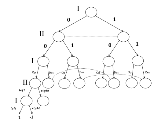
Figure 2: An example of the game $G_{corr}$ where $\ell=2$ and $G$ is a coordination game

Let $\sigma$ be a NE in $G$ in which player $1$’s payoff is no better than it is in any other NE in $G$. Now consider the following simple strategies for the players in $G_{\mathit{corr}}$. Intuitively, the players start by picking a NE in the support of $\pi$ to play, with probability proportional to its coefficient in $\pi$. To this end, fix an ordering of length $\ell$ of the NEs in the support of $\pi$, where each NE appears a number of times proportional to its weight in the convex combination that makes up $\pi$. At the empty history, player $1$ selects an action $a$ uniformly at random from $\{0,\ldots,\ell-1\}$ and puts it in the envelope. Then player $2$ also selects an action $b$ uniformly at random from $\{0,\ldots,\ell-1\}$. Then player $1$ opens the envelope. The players then play the NE in place ($a+b\mod\ell$) in the ordering of NEs. If player $1$ does not open, the players play according to $\sigma$. Call the resulting strategy profile $\vec{\sigma}_{\pi}$. It is not hard to verify that $\vec{\sigma}_{\pi}$ implements $\pi$, and that there exists a probability measure $\mu$ such that $(\vec{\sigma}_{\pi},\mu)$ is a sequential equilibrium of $G_{\mathit{corr}}$. Defining $\mu$ is easy: the only information sets not reached with positive probability (and hence $\mu$ is determined) are the one where “destroy” is played. At that point, the players’ play $\sigma$, so they are best responding to each other, no matter what their beliefs are.

So now all we have to provide is a computational game $\mathcal{G}_{\mathit{corr}}$ that represents $G_{corr}$, where the games in $\mathcal{G}_{\mathit{corr}}$ use cryptography instead an envelope for the first part of the game. Let $d$ be such that $2^{d-1}\leq\ell<2^{d}$. Let $\mathcal{G}_{corr}$ be the sequence where $G_{n}$ is the game where, at the empty history, player $1$ commits to a $d$-bit string by using $d$ commitments in parallel, each with key length $n-1$ and outputs the $d$ commitment strings as his action. Player $2$ then plays a bitstring of length $d$ that can be viewed as a binary representation of a number in $\{0,\ldots,\ell-1\}$. Player $1$ then plays a string that is intended to be the commitment keys of the $d$ commitments. Then the players play a string representing their action in $G$ (again using its binary representation). The utility are then given by the utility functions in $G$.

We now claim that $\mathcal{G}_{corr}$ represents $G_{corr}$.

Theorem 5.1.

$\mathcal{G}_{corr}$ represents $G_{corr}$.

Proof.

It is obvious that $\mathcal{G}_{corr}$ is a computable uniform sequence. We now show that it represents $G_{corr}$. The mappings $\vec{f}$ of histories maps player 1’s commitments to a string $s$ to the action $s\mod\ell$. (Notice that the fact we used $d$ commitments in parallel does not change the fact that the commitments are perfectly binding and thus this is well defined.) Actions of player $2$ are mapped to an action $s\mod\ell$ according to their binary representation; if player 1 reveals $d$ valid keys in $h$, then in $f_{n}(h)$ he plays “open”, and otherwise he plays “destroy”; the actions of $G$ are mapped in the obvious way.

To show that UG4 holds, we proceed as follows: The mapping $\mathcal{F}$ for a player $j$ other than $1$ and $2$ is obvious: It is easy to compute using the TM $R$ of the commitment scheme if the commitments were opened successfully or not, so $j$ can compute at which information set of $G_{corr}$ he is at (given his view), and play the binary representation of the action that the strategy plays at that information set. For player 2, note that player $2$’s first action in $G_{\mathit{corr}}$ can’t depend on player 1’s action, since player 2’s information set contains all the histories. Thus, a deterministic strategy $\sigma_{2}$ for player $2$ in $G_{\mathit{corr}}$ just plays an action in $\{0,\ldots,\ell-1\}$; $\mathcal{F}(\sigma_{2})$ just plays the same action at player 2’s first information set in $\mathcal{G}_{\mathit{corr}}$. Similarly to the other players, $\mathcal{F}(\sigma_{2})$ also plays the same action in $G$ as $\sigma_{2}$ when player 2 is called upon to play again. Given a deterministic strategy $\sigma_{1}$ for player 1, if $\sigma_{1}$ plays $a$ at the first step in $\mathcal{G}_{\mathit{corr}}$, $\mathcal{F}(\sigma_{1})$ chooses uniformly at random one of the $d$-bit strings such that $s=a\mod\ell$ (there are at most $2$ such strings), and plays the commitments strings $C_{1}(1^{n},s_{1},r_{1}),\ldots,C_{d}(1^{n},s_{d},r_{d})$, where $r=r_{1}||\ldots||r_{d}$ is the prefix of the random tape representing the randomness used to compute the commitment strings. To play the action “open”, it computes $k_{i}=C_{2}(1^{n},s_{i},r_{i})$ and play $k_{1}||\ldots||k_{d}$; to play “destroy”, it plays $k_{1}||\ldots||k_{d}\oplus 1$ (a string other than the right keys). Again, it is obvious how player $1$ plays in $G$. It is easy to see that $\mathcal{F}(\vec{\sigma})$ corresponds to $\vec{\sigma}$, so UG4(a) holds. UG4(b) holds for all players trivially given these strategies.

It is also obvious that UG4(c) holds for player $1$. Since the information structure it faces at $\mathcal{G}_{corr}$ and $G_{corr}$ is essentially the same, anything it can do in $\mathcal{G}_{\mathit{corr}}$ can be done by a strategy in $G_{corr}$ by just looking at the distribution of actions in histories that map to each information set.

The other players have different information structures in $\mathcal{G}_{\mathit{corr}}$ and $G_{\mathit{corr}}$, since they see the commitment strings in $\mathcal{G}_{corr}$. We discuss UG4(c) for player 2 here; the argument in the case of the others is similar (and simpler). Let $\sigma_{i}$ for $i\neq 2$ be a strategy for player $i$ in $G_{corr}$, and let $M_{i}=\mathcal{F}(\sigma_{i})$. Let $M^{\prime}$ be an arbitrary polynomial time strategy for player $2$ in $\mathcal{G}_{corr}$, and let $D^{n}_{1}$ be the distribution $M^{\prime}$’s first action in $G_{n}$; let $D^{n}_{j,w}$ be the distribution over the actions of $M^{\prime}$ in $G$ given that the commitment was opened successfully, player $1$ committed to $j$, and player $2$’s first move was $w$; and let $D^{n}_{w}$ be the distribution over the actions of $M^{\prime}$ in $G_{n}$ if the commitment is not opened successfully and player $2$’s first move was $w$. Let $\sigma^{\prime}_{n}$ be a strategy in $G_{\mathit{corr}}$ for player $2$ that plays according to these distributions. We claim that $\{\phi^{G_{n}}_{(M_{1},M^{\prime},\ldots,M_{c})}\}_{n}$ is indistinguishable from $\{\rho^{G_{corr}}_{(\sigma_{1},\sigma^{\prime}_{n},\ldots,\sigma_{c})}\}_{n}$.

Let $\phi^{G_{n},1}_{(M_{1},M^{\prime},\ldots,M_{c})}$ be the distribution over histories ending at the first action of player $2$ when $(M_{1},M^{\prime},\ldots,M_{c})$ is played in $G_{n}$ and mapped using $f_{n}$ to histories of $G_{corr}$, and let $\rho^{G_{corr},1}_{(\sigma_{1},\sigma^{\prime}_{n},\ldots,\sigma_{c})}$ be the distribution over partial histories ending at the first action of player $2$ when $(\sigma_{1},\sigma^{\prime}_{n},\ldots,\sigma_{c})$ is played in $G_{corr}$. We first claim that $\{\phi^{G_{n},1}_{(M_{1},M^{\prime},\ldots,M_{c})}\}_{n}$ is indistinguishable from $\{\rho^{G_{corr},1}_{(\sigma_{1},\sigma^{\prime}_{n},\ldots,\sigma_{c})}\}_{n}$. Assume, by way of contradiction, that it is not. This can happen only if, for infinitely many $n$, $M^{\prime}$ plays some action $a$ with probabilities that differ non-negligibly, depending on whether it is faced with a commitment to different strings $s$ or $s^{\prime}$. But that means that for infinitely many $n$, it can distinguish those two events with non-negligible probability. This contradicts the assumption that the commitment scheme is secure. (Note that it is easy to show that, because a single commitment has the hiding property, then even when $d$ such commitments are run in parallel, no polynomial-time TM should be able to distinguish between commitments to $s$ and $s^{\prime}$.)

It is easy to see that this also means that the distribution over partial histories just before player $2$ plays again are also indistinguishable. Now if the commitment is opened successfully, then the information structure player $2$ faces in $\mathcal{G}_{\mathit{corr}}$ is the same as in $G_{\mathit{corr}}$, and thus the statement is obviously true. If the commitments were not opened, than by using a argument similar to that used for player 2’s first action, we can argue that if the distributions over partial histories just after player $2$ plays again are not indistinguishable, then again we can use that as a distinguisher for the commitment scheme. ∎

By Theorems 4.6 and 5.1, since $\vec{\sigma}_{\mu}$ (with the appropriate beliefs) is a sequential equilibrium of $G_{\mathit{corr}}$, $\mathcal{F}(\vec{\sigma}_{\mu})$ is a computational sequential equilibrium of $\mathcal{G}_{\mathit{corr}}$.

6 Conclusion

The model introduced in this paper is a first step towards a better understanding of polynomially bounded players playing finite games. We defined a sense in which a sequence $\mathcal{G}$ of games represents a single underlying game $G$, gave a novel definition of a computational sequential equilibrium, and provided conditions under which a computational sequential equilibrium (and hence also a computational NE) exists in $\mathcal{G}$. Moreover, the model allows us to separate the cryptographic analysis from the strategic analysis. We show how we can use our model and definitions to analyze complex cryptographic protocols in a way that captures our intuitions about the rational behavior of the players in those protocols.

An important next step is to refine the model so it can capture more complex cryptographic protocols. For example, some cryptographic protocols do not have a unique map between histories and actions (e.g., a computationally binding commitment can map a string to both $0$ or $1$ depending on the key). They also might have abstract actions that are hard to compute (for instance, there might be strings that are not valid commitments at all but it might be hard to compute them), or require a few implementation steps to implement one abstract step. One possible direction is to map a history and the TMs’ views into histories in the game. While this might solve some of the issues raised, it also introduces new challenges, which we intend to investigate.

While in this paper we focus only on computationally bounded players represented by polynomial-time TMs (which seems most appropriate for the cryptographic applications we have in mind), we believe that our approach of relating a sequence of games to a single underlying game, and capturing computational indisitingushability with the information structure of this game can be applied to other models of computations with the appropriate adaptation of computational indisitingushability.

References

- 1 Y. Dodis, S. Halevi, and T. Rabin. A cryptographic solution to a game theoretic problem. In CRYPTO 2000: 20th International Cryptology Conference, pages 112–130. Springer-Verlag, 2000.
- 2 O. Goldreich. Foundations of Cryptography, Vol. 1. Cambridge University Press, 2001.
- 3 S. Goldwasser and S. Micali. Probabilistic encryption. Journal of Computer and System Sciences, 28(2):270–299, 1984.
- 4 R. Gradwohl, N. Livne, and A. Rosen. Sequential rationality in cryptographic protocols. ACM Trans. Econ. Comput., 1(1):2:1–2:38, January 2013.
- 5 J. Y. Halpern, R. Pass, and D. Reichman. On the nonexistence of equilibrium in computational games. 2015.
- 6 J. Y. Halpern, R. Pass, and L. Seeman. Not just an empty threat: subgame-perfect equilibrium in repeated games played by computationally bounded players. In Proc. WINE 2014: 10th Conference on Web and Internet Economics, pages 249–262, 2014.
- 7 J. Y. Halpern, R. Pass, and L. Seeman. The truth behind the myth of the folk theorem. In Proc. 5th Conference on Innovations in Theoretical Computer Science (ITCS ’14), pages 543–554, 2014.
- 8 P. Hubáček, J. B. Nielsen, and A. Rosen. Limits on the power of cryptographic cheap talk. In Advances in Cryptology–CRYPTO 2013, pages 277–297. Springer, 2013.
- 9 P. Hubáček and S. Park. Cryptographically blinded games: leveraging players’ limitations for equilibria and profit. In Proc. 15th ACM Conference on Economics and Computation, pages 207–208, 2014.
- 10 Jonathan Katz. Bridging game theory and cryptography: Recent results and future directions. In Theory of Cryptography, pages 251–272. 2008.
- 11 D. M. Kreps and R. B. Wilson. Sequential equilibria. Econometrica, 50:863–894, 1982.
- 12 M. J. Osborne and A. Rubinstein. A Course in Game Theory. MIT Press, Cambridge, Mass., 1994.
- 13 R. Selten. Spieltheoretische behandlung eines oligopolmodells mit nachfrageträgheit. Zeitschrift für Gesamte Staatswissenschaft, 121:301–324 and 667–689, 1965.
- 14 H. A. Simon. A behavioral model of rational choice. Quarterly Journal of Economics, 49:99–118, 1955.
- 15 A. Urbano and J. E. Vila. Computationally restricted unmediated talk under incomplete information. Economic Theory, 23(2):283–320, 2004.