Spontaneous formation and non-equilibrium dynamics of a soliton-shaped Bose-Einstein condensate in a trap

Abstract

The Bose-stimulated self-organization of a quasi-two dimensional non-equilibrium Bose-Einstein condensate in an in-plane potential is proposed. We obtained the solution of the nonlinear, driven-dissipative Gross-Pitaevskii equation for a Bose-Einstein condensate trapped in an external asymmetric parabolic potential within the method of the spectral expansion. We found that, in sharp contrast to previous observations, the condensate can spontaneously acquire a soliton-like shape for spatially homogenous pumping. This condensate soliton performs oscillatory motion in a parabolic trap and, also, can spontaneously rotate. Stability of the condensate soliton in the spatially asymmetric trap is analyzed. In addition to the nonlinear dynamics of non-equilibrium Bose-Einstein condensates of ultra-cold atoms, our findings can be applied to the condensates of quantum well excitons and cavity polaritons in semiconductor heterostructure, and to the condensates of photons.

I Introduction

Bose-Einstein condensation (BEC) and superfluidity are hallmarks of quantum degenerate systems composed of interacting bosons. In the BEC state, a substantial fraction of particles at low temperatures spontaneously occupies the single lowest-energy quantum state thus, forming a condensate in the energy space. One of famous examples of BECs is a condensation of ultracold alkali-metal atoms at nK range of temperatures Anderson et al. (1995); Davis et al. (1995). The advances ultra-low-temperature techniques have already lead to the development of various technologies including international atomic time keeping, the base of the Global Positioning System, which is familiar to everyone.

Recently, significant progress in solid state physics and nanofabrication has enabled to experimentally create a class of condensed systems in semiconductor heterostructures that demonstrate BEC Butov et al. (2002a); Snoke (2002); Amo et al. (2009). In this case, the Bose particles are excitons, i.e., electron-hole pairs coupled due to Coulomb attraction in quasi-two-dimensional quantum wells (QW), or polaritons, quantum superpositions of excitons and cavity photons (see Carusotto and Ciuti (2013) for extensive review). The effective mass of these particles is much smaller than for their atomic counterpart and it varies from a the free electron mass $m_{e}$ order to $\sim 10^{-4}m_{e}$ depending on the physical realization. As a result, the solid-state systems undergo the BEC transition at much higher temperatures $T_{c}$ than the atomic BEC: $T_{c}$ ranges from $\sim$ a few K to $\sim 40$ K Butov et al. (1994); Snoke (2002); Carusotto and Ciuti (2013). Physics of exciton and polariton BECs has already revealed exciting phenomena including superfluidity Amo et al. (2009), quantized vorticity Lagoudakis et al. (2008), quantum solitons Amo et al. (2011); Sich et al. (2012), and a condensed-matter analogue of Dirac monopole Hivet et al. (2012). Solid-state BEC is a highly developing research field due to potential applications in quantum and optical computing Gibbs et al. (2011); Menon et al. (2010), nonlinear interferometry Sturm et al. (2014), novel light sources Deng et al. (2002), and atomtronics Restrepo et al. (2014). Room temperature BEC has also recently been observed for photons Klaers et al. (2010, 2012). In the latter case, the nonlinear interactions between the light quanta, which are otherwise linear, are provided by the dye molecules introduced into the microcavity.

In this paper, we study the dynamics of a trapped quasi-two-dimensional BEC in the presence of an external source and damping that provides general conditions for the Bose-Einstein condensation of particles with finite lifetime. The reduced dimensionality naturally appears in the solid-state BEC realizations in planar cavities Butov et al. (1994); Snoke (2002); Amo et al. (2009). In trapped atomic BECs this corresponds to the limit case where a characteristic frequency of the trap along one direction is much higher to those in two other directions Dalfovo et al. (1999). To capture the experimental conditions with spatially asymmetric traps, the condensate dynamics was considered for elliptic traps where the trapping potential strengths in two orthogonal directions are not the same. In our studies, we perform the simulations taking an exciton condensate as a relevant example.

We report that, in sharp contrast to previous observations, under certain conditions the condensate spontaneously self-localizes in a form of a solitary wave with a size smaller than a typical condensate cloud size and smaller than the excitation spot size. We found that a few types of the soliton-like waves can form, including condensate humps and rotating doughnut condensates (rings). Earlier, the solitons propagating on the background of a uniform condensate has been observed in quasi-two-dimensional solid-state systems Amo et al. (2011); Sich et al. (2012). In those studies the solitons were the condensate perturbations, which have been created artificially by perturbing the condensate density by an additional “writing” laser beam. In our work, the condensate itself self-organizes into a strongly nonuniform soliton-shaped state that behaves as a “particle”. This particle travels in a trap much like a classical particle that oscillates in an external parabolic potential. Self-organization of the condensate into a soliton is caused by the interplay of the Bose-stimulated condensate formation and the nonlinear interactions between the Bose particles that is, by the universal factors, which are present in any physical realization of a BEC. It was also found that if the eccentricity of the elliptic parabolic trap is high, the solitary wave does not form. In the latter case, a conventional fluctuating condensate, which fills all the energetically accessible area in the trap, was formed Vörös et al. (2006); Berman et al. (2012a, b).

The paper is organized as follows. In Sec. II we describe the model used in the simulations and present the method of solution of the nonlinear, driven-dissipative Gross-Pitaevskii equation for a BEC trapped in an external asymmetric parabolic potential. In Sec. III we discuss our main findings. Our conclusions follow in Sec. IV.

II Theoretical framework

In this section we describe our research methodology and present the system parameters, for which the simulations have been done. To describe the dynamics of the dipolar exciton condensate, we utilize the driven-dissipative Gross-Pitaevskii equation for the condensate wave function. In this work, we take excitons in coupled semiconductor quantum wells, i.e. dipolar excitons, as a physical realization of non-equilibrium Bose-Einstein condensate where nonlinearity plays an important role Butov et al. (1994, 2002b, 2002a); Snoke et al. (2002); Negoita et al. (1999); High et al. (2012).

The Gross-Pitaevskii equation also captures the dynamics of Bose-Einstein condensates of cavity polaritons Carusotto and Ciuti (2013) and of ultra-cold atoms Pitaevskii and Stringari (2003). In the latter case, the complex terms in the right-hand side of driven-dissipative Gross-Pitaevskii equation, Eq. (1) below, correspond to the slow condensate depletion due to the cloud evaporation and to the initial injection of relatively hot atoms. The effective interaction strength in quasi-two-dimensional atomic condensates depends on the condensate density Pitaevskii and Stringari (2003) in analogy with the case of dipolar exciton condensates detailed in this Section below.

The model formulated below captures the realistic details of pumping in the Bose-Einstein condensed systems. Specifically, the particles are injected into the system at elevated energies (frequencies) and then relax to the low-energy states due to the nonlinear interaction with each other. The relevant examples of such systems are mentioned in the Introduction. For example, for the dipolar exciton condensates, the excitons are created at relatively high energies due to coupling of hot electrons and holes generated by the external laser radiation Damen et al. (1990). For polaritonic condensates, the scattering into the condensate from a thermal bath of non-condensed polaritons occurs at the bottleneck energy scale, which significantly exceeds the characteristic energies of the particles in the ground state Carusotto and Ciuti (2013). In trapped atomic condensates, relatively hot atoms with the energies exceeding the ground-state energy in the trapping potential are initially injected into the system. It has already been demonstrates that in the case of the dipolar exciton condensates, the account for these details results in formation of condensate turbulence under certain conditions Berman et al. (2012a, b). In this paper we show that this model also predicts formation of long-living, soliton-like coherent structures in the condensate. In contrast, in the conventional approach (see, e.g. Ref. Carusotto and Ciuti (2013) for review), the pump rate does not depend on the particle energy thus, the important details of the nonequilibrium dynamics of the condensates are omitted.

II.1 Driven-dissipative Gross-Pitaevskii equation for two-dimensional condensates

At temperatures below the BEC transition temperature, the dipolar exciton condensate is described by the mean-field wave function $\Psi=\Psi(\bm{r},t)$, which depends on the two-dimensional radius vector in the QW plane $\bm{r}=(x,y)$ and time $t$. The time evolution of the condensate wave functions in an external trap is captured by the Gross-Pitaevskii equation

$$i\hbar{\frac{\partial\Psi}{\partial t}}=-{\frac{\hbar^{2}}{2m_{ex}}}\Delta\Psi+U(\bm{r})\Psi+g\Psi|\Psi|^{2}+i\hbar{\left(\hat{R}-{\frac{1}{2\tau}}\right)}\Psi.$$ (1)

In Eq. (1), $m_{ex}$ is the exciton mass, $\Delta$ is the two-dimensional Laplacian operator in the QW plane. The parabolic trapping potential for the dipolar excitons is $U(\bm{r})={\frac{1}{2}}\left(\gamma_{x}x^{2}+\gamma_{y}y^{2}\right)$, where $\gamma_{x}$ and $\gamma_{y}$ are the potential strengths in $x$ and $y$ directions, respectively. The last term in Eq. (1) describes creation of the excitons due to the interaction with the laser radiation and exciton decay, $\tau$ is the exciton lifetime. The source term $\propto\hat{R}\Psi(\bm{r},t)$ reflects the fact that the condensate particle creation rate $\sim\partial|\Psi(\bm{r},t)|^{2}/\partial t$ due to Bose-stimulated scattering into the condensate is proportional to the condensate density $|\Psi(\bm{r},t)|^{2}$. The effective interaction strength $g$ in Eq. (1) for the dipolar exciton condensate depends on the chemical potential $\mu$ in the system Berman et al. (2012a, b). In the case where the exciton cloud size is much greater than the mean exciton separation, the interaction strength is $g=2\pi(e^{4}D^{4}\mu/\epsilon^{2})^{1/3}$, where $e$ is the electron charge, $D$ is the interwell distance, $\epsilon$ is the dielectric constant of the material in the gap between two quantum wells Berman et al. (2012a, b).

To study the exciton condensate dynamics, we numerically integrate Eq. (1). There are numbers of approaches for the numerical integration of Gross-Pitaevskii-type equations. One of the approaches is in solving Eq. (1) in $\mathbf{r}$-space by discretizing it using a Crank-Nicholson finite difference scheme Ruprecht et al. (1995); Adhikari (2000); Adhikari and Muruganandam (2002). In Refs. Cerimele et al., 2000 and Bao and Tang, 2003 the ground-state wave function of a trapped BEC was found by the direct minimization of the energy functional for the Gross-Pitaevskii equation. The convergence of various methods has been studied in Refs. Sanz-Serna, 1984 and Sanz-Serna and Verwer, 1986. The stability and time-evolution of solutions of the driven-dissipative multidimensional Gross-Pitaevskii equation has recently been analyzed numerically in Ref. Moxley et al., 2015. The spectral representation of the Gross-Pitaevskii equation has been considered for atomic BEC condensates without a trap Dyachenko and Falkovich (1996). In that case, the condensate wave function was expanded using the plane-wave basis. Comprehensive reviews for these methods are given in Refs. Antoine et al., 2013 and Kolmakov et al., 2014.

In our approach, we use the spectral representation for the condensate wave function $\Psi(\bm{r},t)$ by expanding it in terms of basis functions of the exactly solvable stationary eigenvalue problem and for the time-dependent coefficients of the expansion obtain the system of the first-order differential equations that we solve numerically.

To utilize our approach let us consider the linear Hermitian part of the Hamiltonian of Eq. (1)

$$\hat{H}_{0}=-{\frac{\hbar^{2}}{2m_{ex}}}\left({\frac{\partial^{2}}{\partial x^{2}}}+{\frac{\partial^{2}}{\partial y^{2}}}\right)+{\frac{1}{2}}\left(\gamma_{x}x^{2}+\gamma_{y}y^{2}\right),$$ (2)

which is the Hamiltonian of a two-dimensional asymmetric harmonic oscillator. This Hamiltonian enables the variable separation and factorization of the wave functions Messiah (1961),

$$\hat{H}_{0}\psi_{n_{x}}(x)\psi_{n_{y}}(y)=E_{n_{x}n_{y}}\psi_{n_{x}}(x)\psi_{n_{y}}(y),$$ (3)

where $E_{n_{x}n_{y}}=E_{n_{x}}^{\lambda_{x}}+E_{n_{y}}^{\lambda_{y}}$, $E_{n_{x}}^{\lambda_{x}}=\hbar\omega_{n_{x}}^{\lambda_{x}}$ and $E_{n_{y}}^{\lambda_{y}}=\hbar\omega_{n_{y}}^{\lambda_{y}}$ determine the oscillator eigen frequencies $\omega_{n_{x}}^{\lambda_{x}}$ and $\omega_{n_{y}}^{\lambda_{y}}$ in $x-$ and $y-$direction, respectively. The functions $\psi_{n_{x}}^{\lambda_{x}}(x)$ and $\psi_{n_{y}}^{\lambda_{y}}(y)$ are the eigenfunctions of a classical one-dimensional harmonic oscillator problem that obey the time-independent Schrödinger equation

$$-{\frac{\hbar^{2}}{2m_{ex}}}{\frac{d^{2}\psi_{n_{\xi}}(\xi)}{d\xi^{2}}}+{\frac{1}{2}}\gamma_{\xi}\xi^{2}\psi_{n_{\xi}}(\xi)=\hbar\omega_{n_{\xi}}\psi_{n_{\xi}}(\xi),$$ (4)

where $\xi$ labels the $x$ and $y$ variables. The solution of Eq. (4) is Messiah (1961)

$$\psi_{n_{x}}^{\lambda_{x}}(x) = {\frac{1}{\sqrt{\lambda_{x}}}\frac{1}{\sqrt{\pi^{1/2}2^{n_{x}}n_{x}!}}}e^{-\frac{1}{2}\left(\frac{x}{\lambda_{x}}\right)^{2}}H_{n_{x}}\left(\frac{x}{\lambda_{x}}\right)\text{, \ }$$ (5)

$$\psi_{n_{y}}^{\lambda_{y}}(y) = {\frac{1}{\sqrt{\lambda_{y}}}\frac{1}{\sqrt{\pi^{1/2}2^{n_{y}}n_{y}!}}}e^{-\frac{1}{2}\left(\frac{y}{\lambda_{y}}\right)^{2}}H_{n_{y}}\left(\frac{y}{\lambda_{y}}\right),$$ (6)

where $\omega_{n_{x}}^{\lambda_{x}}=(\gamma_{x}/m_{ex})^{1/2}(n_{x}+1/2)$, $\omega_{n_{y}}^{\lambda_{y}}=(\gamma_{y}/m_{ex})^{1/2}(n_{y}+1/2)$, $n_{x}=0,1,2,\ldots$, $n_{y}=0,1,2,\ldots$,  $H_{n}$ are the Hermite polynomials, and $\lambda_{x}$ and $\lambda_{y}$ characterize the oscillator length scales in the $x$ and $y$ directions, respectively.

To capture the presence of the trap now let us expand the condensate wave function $\Psi(\bm{r},t)$ in terms of the eigenfunctions $\psi_{\bm{n}}(\bm{r})=\psi_{{n_{x}}}^{\lambda_{x}}(x)\psi_{{n_{y}}}^{\lambda_{y}}(y)$

$$\Psi(\bm{r},t)=\sum_{\bm{n}}A_{\bm{n}}(t)\psi_{\bm{n}}(\bm{r}),$$ (7)

where $A_{\bm{n}}(t)$ are the time-dependent coefficients of the expansion, and $\bm{n}=(n_{x},n_{y})$ is a two-dimensional integer index.

After the substitution of the expansion (7) into Eq. (1) one obtains the following system of the first-order differential equations for the coefficients $A_{\bm{n}}(t)$,

$$i\hbar{\frac{\partial A_{\bm{n}}(t)}{\partial t}} = \hbar\omega_{\bm{n}}A_{\bm{n}}(t)+i\hbar\sum_{\bm{m}}R_{\bm{n}\bm{m}}A_{\bm{m}}(t)-i{\frac{\hbar}{2\tau}}A_{\bm{n}}(t)$$ (8)

$$+ g\sum_{\bm{m},\bm{p},\bm{q}}W_{\bm{n}\bm{m}\bm{p}\bm{q}}A_{\bm{m}}(t)A_{\bm{p}}(t)A_{\bm{q}}^{\ast}(t),$$

where

$$W_{\bm{n}\bm{m}\bm{p}\bm{q}}=\lambda_{0}^{2}w_{n_{x}m_{x}p_{x}q_{x}}w_{n_{y}m_{y}p_{y}q_{y}},$$

$$w_{nmpq}=\int_{-\infty}^{\infty}\!d\xi\,f_{n}(\xi)f_{m}(\xi)f_{p}(\xi)f_{q}(\xi),$$

and

$$f_{n}(\xi)={\frac{1}{\sqrt{\pi^{1/2}2^{n}n!}}}e^{-\xi^{2}/2}H_{n}(\xi).$$

The matrix elements of the source operator $\hat{R}$ in Eq. (11) are

$$R_{\bm{n}\bm{m}}=\int d\bm{r}\,\psi_{\bm{n}}^{\ast}(\bm{r})\hat{R}\psi_{\bm{m}}(\bm{r}).$$ (9)

We consider the case where the excitons are created by an external homogenous source in a given range of energies $(\hbar\omega_{1},\hbar\omega_{2})$, where $\omega_{1}$ and $\omega_{2}$ are the boundary frequencies of the excitation frequency range. Thus, we assume the following form for the matrix elements (9),

$$R_{\bm{n}\bm{m}}=\delta_{\bm{n}\bm{m}}\Delta(\omega_{\bm{n}}),$$ (10)

where $\Delta(\omega_{\bm{n}})=R_{0}$ if $\omega_{1}\leq\omega_{\bm{n}}\leq\omega_{2}$ and $\Delta(\omega_{\bm{n}})=0$ otherwise. The $R_{0}$ constant characterizes the intensity of the exciton source. In most simulations, it was set equal $R_{0}=0.15\omega_{0}$ where $\omega_{0}=(\gamma_{0}/m_{ex})^{1/2}$ is the oscillatory unit of frequency. Additionally, the simulations have been performed for $R_{0}=0.25\omega_{0}$ to demonstrate the transition to turbulence at elevated pump rates. In the simulations, we set $\omega_{1}=5\omega_{0}$ and $\omega_{2}=7\omega_{0}$.

We consider Eqs. (1) and (8) in the interaction representation by separating the time dependence for the linearized equation, $A_{\bm{n}}(t)=a_{\bm{n}}(t)e^{-i\omega_{\bm{n}}t}$, where $\omega_{\bm{n}}$ is the eigenfrequency of the mode $\bm{n}$. In this representation, Eq. (8) reads

$$i\hbar{\frac{\partial a_{\bm{n}}(t)}{\partial t}} = i\hbar\left(R_{\bm{n}\bm{n}}-{\frac{1}{2\tau}}\right)a_{\bm{n}}(t)$$ (11)

$$+ g\!\!\!\sum_{\bm{m},\bm{p},\bm{q}}\!\!\!W_{\bm{n}\bm{m}\bm{p}\bm{q}}\,a_{\bm{m}}(t)a_{\bm{p}}(t)a_{\bm{q}}^{\ast}(t)e^{i\Delta\omega t},$$

where $W_{\bm{n}\bm{m}\bm{p}\bm{q}}$ are the matrix elements of the dipolar exciton interaction, $\Delta\omega=\omega_{\bm{q}}+\omega_{\bm{n}}-\omega_{\bm{m}}-\omega_{\bm{p}}$ is the frequency detuning, and a star stands for the complex conjugate.

The characteristic length scales of the linearized problem are

$$\lambda_{x}=\left({\frac{\hbar^{2}}{m\gamma_{x}}}\right)^{1/4},\quad\lambda_{y}=\left({\frac{\hbar^{2}}{m\gamma_{y}}}\right)^{1/4}.$$ (12)

We assume that the trap is elongated in $x$ direction thus, $\lambda_{x}\geq\lambda_{y}$. The characteristic trapping potential length scale is $\lambda_{0}=\sqrt{\lambda_{x}\lambda_{y}}$ and the mean trapping potential strength is $\gamma_{0}=\sqrt{\gamma_{x}\gamma_{y}}$. To characterize the spatial asymmetry of the trapping potential $U(\bm{r})$ we introduce its eccentricity as follows,

$$\varepsilon=\sqrt{\frac{\lambda_{x}^{2}-\lambda_{y}^{2}}{\lambda_{x}^{2}}}.$$ (13)

While the dependence of the condensate dynamics is studied for different eccentricities $\varepsilon$, the total area accessible for the exciton cloud $S=\pi\lambda_{0}^{2}$ in the trap $U(\bm{r})$ is fixed to keep the average condensate density constant at a given particle creation rate.

The trap parameters $\gamma_{x}$ and $\gamma_{y}$, which represent the confinement strength, are expressed through the eccentricity (13) as

$$\gamma_{x}=\gamma_{0}(1-\varepsilon^{2}),\quad\gamma_{y}={\frac{\gamma_{0}}{1-\varepsilon^{2}}}.$$ (14)

The characteristic length scales in the $x$ and $y$ directions are

$$\lambda_{x}={\frac{\lambda_{0}}{(1-\varepsilon^{2})^{1/4}}},\quad\lambda_{y}={\lambda_{0}(1-\varepsilon^{2})^{1/4}}.$$ (15)

The eigenfrequency of the oscillatory mode $\bm{n}=(n_{x},n_{y})$ in a trap with the eccentricity $\varepsilon$ is

$$\omega_{\bm{n}}= \left({\frac{\gamma_{0}}{m_{ex}}}\right)^{1/2}\left[\sqrt{1-\varepsilon^{2}}(n_{x}+1/2)\right.$$ (16)

$$+\left.{\frac{1}{\sqrt{1-\varepsilon^{2}}}}(n_{y}+1/2)\right].$$

The initial conditions at $t=0$ were set as a Rayleigh-Jeans-like thermal distribution

$$a_{\bm{n}}(0)=\left({\frac{k_{B}T}{\mu_{0}+\hbar\omega_{\bm{n}}}}\right)^{1/2}e^{i\phi_{\bm{n}}}$$ (17)

with the chemical potential $\mu_{0}=\hbar\omega_{0}$, random phases $\phi_{\bm{n}}$ and the temperature $T=0.1\hbar\omega_{0}/k_{B}$, where $k_{B}$ is the Boltzmann constant.

II.2 Simulation parameters and the integration method

As we stated above, we consider dipolar excitons with spatially separated electrons and holes as the main example of non-equilibrium Bose-Einstein condensation Butov et al. (1994, 2002b, 2002a); Snoke et al. (2002); Negoita et al. (1999); High et al. (2012). Taking GaAs heterostructures as a relevant example of such system, we set the dielectric constant equal $\epsilon=13$. The simulations have been done for $\gamma_{0}=50$ eV/cm², the exciton mass $m_{ex}=0.22m_{e}$ where $m_{e}$ is the free electron mass, the interwell distance $D=4.2$ nm, and the exciton lifetime $\tau=100$ ns, which are the representative parameters for the experiments with the dipolar excitons in GaAs coupled QWs Negoita et al. (1999); Vörös et al. (2006); High et al. (2012). In the simulations, we express the spatial coordinates and time in the oscillatory units of length $\Delta x\equiv\lambda_{0}=0.9$ $\mu$m and of time $\Delta t=(m_{ex}/\gamma_{0})^{1/2}=1.6$ ns. The unit of frequency in the simulations is $\omega_{0}=\Delta t^{-1}=6.3\times 10^{8}$ s^-1.

As it is detailed above, we consider the dipolar exciton condensates under the conditions of the experiments in Refs. Butov et al., 1994, 2002b, 2002a; Snoke et al., 2002; Negoita et al., 1999; High et al., 2012 where a rarefied exciton gas with the density of $n_{2D}\sim 10^{9}-10^{10}$ cm^-2 is formed in coupled QWs with the interwell separation $D>0.3a_{B}$, where $a_{B}=\epsilon\hbar^{2}/2m_{r}e^{2}\approx 7$ nm is the two-dimensional exciton Bohr radius and $m_{r}$ is the exciton reduced mass. Such dilute electron-hole system ($a_{B}n_{2D}^{-1/2}\ll 1$) can be described as a weakly-non-ideal Bose-gas of excitons Keldysh and Kozlov (1968); Moskalenko and Snoke (2000). As it was shown in Refs. Schindler and Zimmermann, 2008 and Laikhtman and Rapaport, 2009, in this regime a gas of interacting dipolar excitons can be considered as a quantum fluid and the probability of biexciton formation is negligibly small.

We numerically integrated Eq. (11) with the 4th order Runge-Kutta scheme with the time step of $10^{-2}\Delta t$. To obtain the relative accuracy better than $10^{-3}$ for the condensate wave function and the relative accuracy of $4\times 10^{-5}$ for the total number of excitons in the condensate, we use $N_{x}\times N_{y}=256$ basis functions in the expansion (7) where $0\leq n_{x}<N_{x}$, $0\leq n_{y}<N_{y}$, and $N_{x}=N_{y}=16$ Gothandaraman et al. (2011, DOI 10.1109/SAAHPC.2011.32).

In the present work, we utilized Graphics Processing Unit (GPU) NVIDIA Tesla K20m Nvi to solve numerically Eqs. (11). The use of GPUs enabled us to perform the simulations within a practically reasonable amount of time and to achieve the required accuracy. In the GPU implementation, we separated the real and imaginary parts in Eqs. (11) and thus, obtained a set of real equations. The interaction amplitudes $W_{\bm{n}\bm{m}\bm{p}\bm{q}}$ and the coefficients $a_{\bm{n}}(0)$ were initialized on the host (processor) and then, were transferred from the host memory to the device (GPU) memory prior to the start of the integration. In the GPU implementation of the code, we used a two-dimensional (2D) computational grid consisting of 2D blocks, which in their turn consisted of a set of threads that worked in parallel. We divided the problem size, $N_{x}\times N_{y}$, in such a way that each thread on GPU operated on one element of the resultant grid that is, updated the variables at given $(n_{x},n_{y})$ at the current time step.

It follows from Eqs. (11) that for each $\bm{n}$, the nonlinear interaction term involves a summation over six one-dimensional indices. Given the 2D computational grid, if each thread in a block would access the GPU memory to read the data, the performance of the kernel would suffer from the memory bandwidth bottleneck in addition to the read latency. To effectively utilize the memory bandwidth and avoid redundant read accesses, we performed the following optimizations. The GPU kernel has been divided into three sub-kernels, which performed partial summations in the nonlinear term of Eqs. (11). The first sub-kernel produced the summation over the two-dimensional index $\bm{q}$. The output of this kernel has been stored in the global memory on the device and then, has been used by the second partial summation sub-kernel to produce the partial sum over the index $\bm{p}$. The latter partial sum was used by the third sub-kernel to produce the final sum in the nonlinear term in Eqs. (11). It was found that splitting the summation kernel into three sub-kernels results in lower execution time than performing the complete summation in a single kernel.

We used a serial code for the same parameter set to benchmark the GPU code. In the serial code, the explicit complex representation of Eqs. (11) has been utilized. We found that the simulation for a single run required $\sim 88$ hours on a GPU and showed $\sim 10\times$ acceleration compared to the serial version of the code.

III Results and Discussion

In this section we present the results of our studies. First, we consider spontaneous formation of the dipolar exciton condensate patterns and their dynamics in a trapping potential. Then, we analyze the details of the pattern rotation. Finally, we consider the effect of the asymmetry of the trapping potential and compare our findings with the existing results.

III.1 Formation of a soliton-like condensate

To study the dynamics of the dipolar exciton condensate, we determined the condensate density distribution at different moments of time by integrating Eq. (1) with the source term (10) and initial conditions (17). In our studies, we performed six independent runs for the trap eccentricity $\varepsilon=0.2$ and three independent runs for all other values of the eccentricity in the range $0\leq\varepsilon\leq 0.8$. Fig. 1 demonstrates the dependence of the total number of dipolar excitons in the condensate as a function of time,

$$N(t)=\int d^{2}\bm{r}|\Psi(\bm{r},t)|^{2},$$ (18)

obtained in the simulations for the trap eccentricity $\varepsilon=0.2$. It is seen that initially the number of excitons grows with time and then, saturates at $t>t_{s}\equiv 70\Delta t\approx 1.1\times 10^{-7}$ s. At $t\sim t_{s}$ the system comes to a steady state where the total number of dipolar excitons only slowly varies with time.

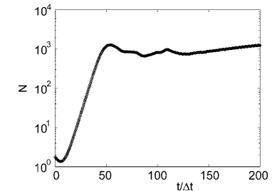
Figure 1: Dependence of the total number of dipolar excitons in the condensate on time in a trap with $\gamma_{0}=50$ eV/cm² for the trap eccentricity $\varepsilon=0.2$. The numerical unit of time $\Delta t$ is specified in the text.

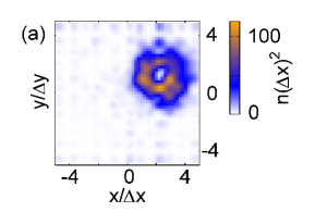
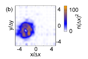
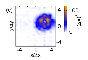
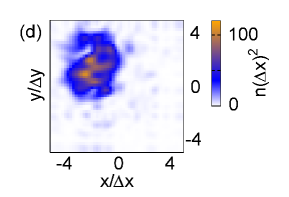
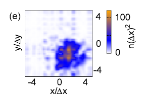
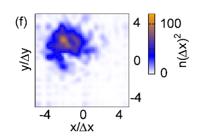
Figure 2: (Color online) Formation of a traveling soliton-like dipolar-exciton pattern in a trap with the eccentricity $\varepsilon=0.2$ (upper row) and $\varepsilon=0$ (lower row). The figures show the exciton condensate density $n(\bm{r},t)=|\Psi(\bm{r},t)|^{2}$ in three subsequent moments. Upper row: (a) $t=139.5\Delta t$, (b) $t=142.5\Delta t$, and (c) $t=145.5\Delta t$ after the external drive was turned on. Lower row: (d) $t=143.0\Delta t$, (e) $t=146.5\Delta t$, and (f) $t=149.5\Delta t$. The vertical bars show the exciton condensate density. The numerical unit of length $\Delta x$ is specified in the text.

To characterize the dipolar exciton condensate dynamics in the steady state at $t>t_{s}$, we studied the time evolution of the condensate density in the trap. Fig. 2 shows the graphical output from the simulations made for the eccentricity $\varepsilon=0.2$ (upper row) and $\varepsilon=0$ (lower row). The results in Fig. 2a-c are shown for the same data with $\varepsilon=0.2$ as in Fig. 1 above. It is seen in Fig. 2 that in both cases $\varepsilon\neq 0$ and $\varepsilon=0$, a spatially-localized condensate pattern is formed. Below we refer to such structures as condensate solitary waves, or condensate solitons.

Figure 3: Motion of (a) $x$- and (b) $y$-coordinates of the center of mass of the condensate pattern. Figure (c) shows motion of the center of mass of the condensate in the $(x,y)$ plane for $t\geq 150\Delta t$, where the pattern exhibits stable periodic oscillations in the parabolic trap. The eccentricity of the trapping potential is $\varepsilon=0.2$. The curves in figures a-c are shown for the data in Fig. 2a-c.

It is also seen in Fig. 2, the pattern travels in the trapping potential. To characterize the condensate pattern motion, we show in Fig. 3a,b the dependence on time of the $x$ and $y$ coordinates of the center of mass of the dipolar exciton condensate for the data presented in Fig. 2a-c. The center-of-mass coordinate $\bm{r}_{cm}(t)=(x_{cm}(t),y_{cm}(t))$ was calculated from the condensate wave function as follows

$$\bm{r}_{cm}(t)=\frac{\int d^{2}\bm{r}|\Psi(\bm{r},t)|^{2}\bm{r}}{\int d^{2}\bm{r}|\Psi(\bm{r},t)|^{2}}.$$ (19)

It is seen from Fig. 3a,b that the position of the center of mass of the pattern oscillates with time. At the moment $t\sim 130\Delta t$, the oscillations reach a steady state, in which their amplitude and period only slowly varies with time. As follows from Fig. 3a,b, the period of the oscillation of the pattern in the trap is $\sim 6.3\Delta t\approx 1.0\times 10^{-8}$ s. The trajectory of the pattern can also be viewed as a Lissajous figure for the condensate center of mass in a parametric plot in the $(x_{cm}(t),y_{cm}(t))$ plane, as it is presented in Fig. 3c. The distance between two farthest points of the trajectory for the condensate center of mass estimated from Fig. 3a-c is $\sim 4.8\Delta x\approx 4.3$ $\mu$m.

Figure 4: Time-averaged radial density distribution (20) of the dipolar exciton condensate soliton as a function of the radial distance $\rho$ in the center-of-mass frame for three independent runs with the eccentricity $\varepsilon=0$ (open circles and open triangles) and for $\varepsilon=0.2$ (filled triangles). The averaging is made for the time period between the moments $t_{1}=100\Delta t$ and $t_{2}=200\Delta t$. Data for $\varepsilon=0$ (open circles) and $\varepsilon=0.2$ (filled triangles) are calculated for the data shown in Fig. 2 in the upper and lower rows, respectively. Points show the result of the calculation, curves are shown to guide the eye.

To characterize the internal structure of the soliton-like pattern, we calculated the time- and angle-averaged radial density distribution function for the condensate in the center-of-mass frame,

$$D(\rho)={\frac{1}{t_{2}-t_{1}}}\int_{t_{1}}^{t_{2}}dt\left({\frac{1}{2\pi}}\int_{0}^{2\pi}d\varphi_{\bm{\rho}}|\Psi(\bm{r}_{cm}(t)+\bm{\rho},t)|^{2}\right).$$ (20)

In Eq. (20), $(t_{2}-t_{1})$ is the time-averaging interval, the integral in the round brackets is taken over the direction $\varphi_{\bm{\rho}}$ of the relative radius-vector $\bm{\rho}=\bm{r}-\bm{r}_{cm}(t)$, and we denoted $\rho=|\bm{\rho}|$. The time-averaging interval was bound by the moments $t_{1}=140\Delta t$ and $t_{2}=200\Delta t$. The results of the calculations for three independent runs for $\varepsilon=0$ and $\varepsilon=0.2$ are shown Fig. 4. It is seen that the characteristic radius $\rho_{0}$ of the pattern defined as a width at the half height for $D(\rho)$ varies from $\sim 2\Delta x$ to $2.5\Delta x$. This conclusion was validated for all independent runs performed under the same conditions. The comparison of Figs. 3a-c and Fig. 4 shows that the traveled distance for the soliton-like pattern during its oscillation in the trap is of the order of or greater than twice the radius of the pattern. In other words, a soliton-like pattern performs large-amplitude oscillatory motion in a parabolic trap.

It is also seen in Fig. 4 that two types of patterns are formed. In the pattern of the first kind, the maximum of the exciton condensate density is positioned at its center $\bm{r}_{cm}$ (see open circles in Fig. 4). This corresponds to a hump-like soliton structure. In the pattern of the second kind, the condensate density has a minimum at the center of the pattern (open triangles and filled triangles in Fig. 4) and therefore, it corresponds to a ring-like structure. We also found that the structures of both kinds can be formed for the same eccentricity (cf. open circles and open triangles for $\varepsilon=0$ in Fig. 4). It is worth noting that the runs are independent since each run was set based on random phases in the initial conditions for the condensate wave function at $t=0$ as described in Sec. II.1. The motion of a ring structure is shown in the first row of Fig. 2, for which the minimum of the condensate density is seen as a bright spot at the center of the pattern, whereas a hump-like structure is shown in the second row of the same figure.

We infer that the solitary-wave condensate formation is caused by the interplay of the two factors: (i) Bose-stimulated scattering of excitons into the condensate and (ii) the exciton-exciton repulsion in the condensate. The first factor results in the increased probability $\propto n_{i}$ of the condensate growth in the state $i$ in the region already occupied by $n_{i}$ particles Snoke (2009). This effect is captured by the source term in Eq. (1) as explained in Sec. II.1. It leads to the exponential-like increase of the particle occupation numbers in the occupied states. However, if the spatial density of the condensate is increased, the mutual repulsion of the condensate particles tends to decrease the density and results in “spreading” of the particles over the system. The nonlinear term in Eq. (1) is responsible for this effect. In the presence of the continuous source of the particles (i.e., external laser radiation), this is the finite lifetime of dipolar excitons that limits the growth of the total number of the particles in the condensate. The approach where the particles are injected into the system at a given energy scale has earlier been used to describe the dynamics of the Bose-Einstein condensation of ultra-cold gases Dyachenko and Falkovich (1996); Lvov et al. (2003); Zakharov and Nazarenko (2005) (see Ref. Kolmakov et al., 2014 for review). Specifically, in that scenario, the injected hot atoms relaxed due to multiple collisions toward the condensate state. The condensate depletion due to atom evaporation was captured by introducing the effective condensate decay rate. In contrast, for the case of dipolar exciton condensate considered in this paper, the depletion rate is set the same for all states to capture the fact that the dipolar exciton lifetime only weakly depends on the exciton energy.

Figure 5: (a) Dependence of the angular momentum of the ring structure in Fig. 2a-c on time. Points show the results of the calculation, the line segments between the points are shown to guide the eye. The momentum is expressed in the units of $\hbar$. (b) The time-dependence of the probabilities $|c_{m}(t)|^{2}$ of having the momentum $m$. (c) Time-averaged probabilities, $\langle|c_{m}(t)|^{2}\rangle$, for various momenta $m$. The graphs in a-c are plotted for the data shown in Fig. 2a-c

III.2 Ring condensate rotation

We assume that formation of the ring structures is caused by spontaneous rotation of the non-equilibrium condensate. It is known that for the Bose-condensed, superfluid systems two types of rotation are possible: (i) vortex rotation and (ii) solid-body-like rotation Khalatnikov (1965). The vortex rotation is realized as quantized vortices in the condensate. The latter have a velocity singularity and zero condensate density at the vortex core Gross (1961). In addition to classical experiments with superfluid He-II (see, e.g., a review in Ref. Andronikashvili et al., 1961), quantized vortices have recently been observed in Bose-Einstein condensates of ultra-cold atoms Weiler et al. (2008) and in condensates of exciton polaritons Lagoudakis et al. (2008); Manni et al. (2011); Keeling and Berloff (2008). For the solid-body rotation, the condensate density does not mandatory turn to zero at the rotation center Khalatnikov (1965). Below we demonstrate that the solid-body rotation is realized for the soliton-like patterns described above.

To analyze the rotation of the pattern we, first, calculate the angular momentum of the dipolar exciton condensate as a function of time

$$M(t)=\int d^{2}\bm{r}\Psi^{\ast}(\bm{r},t)\hat{M_{z}}\Psi(\bm{r},t),$$ (21)

where

$$\hat{\bm{M}}=[\bm{\rho}\times\hat{\bm{p}}]$$

is the angular momentum operator for the condensate in the center-of-mass frame, $\hat{\bm{p}}=-i\hbar\nabla_{\bm{\rho}}\equiv-i\hbar\frac{\partial}{\partial\bm{\rho}}$ is the linear momentum operator, and $z$ marks the direction perpendicular to the QW plane. Fig. 5a demonstrates the time dependence of the angular momentum of the ring pattern shown in Fig. 2a-c. We see in Fig. 5a that the angular momentum of the ring pattern fluctuates with time. We note that the angular momentum fluctuations are natural for the dipolar exciton condensate since the system is driven by an external pump: according to Eq. (1) both the source and damping of the excitons are present. Additionally, the ring condensate is formed in the parabolic trap that breaks the rotational symmetry in the moving, off-center frame of reference. Therefore, the angular momentum of the system is not conserved. However, it is seen in Fig. 5a that at the moment of time $t\approx 140\Delta t$ the angular momentum relaxes to a steady state and it further fluctuates about the mean value $M\approx 0.8$.

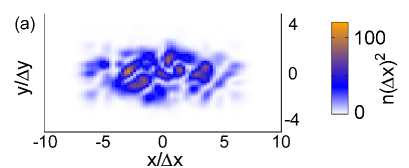
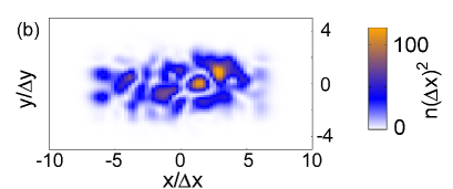
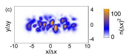
Figure 6: (Color online) Exciton density distribution in a trap with the eccentricity $\varepsilon=0.8$ for the moments (a) $t=139.5\Delta t$, (b) $t=142.5\Delta t$, and (c) $t=145.5\Delta t$. The vertical bars show the exciton condensate density $n(x,y)$. It is seen that a traveling exciton pattern does not emerge for a large eccentricity $\varepsilon$, and a turbulent condensate Berman et al. (2012a, b) is formed instead.

To more fully characterize the pattern rotation, we calculated the time dependence of the probabilities $|c_{m}(t)|^{2}$ of having the specific angular momentum $m$. Here, $c_{m}(t)$ are the normalized components the expansion of the exciton condensate wave function over the basis functions with a fixed momentum $m$ in the center-of-mass frame,

$$c_{m}(t)=\frac{\displaystyle\int d\varphi_{\bm{\rho}}d\rho\,\rho\Psi(\bm{r},t)\Phi_{m}^{*}(\varphi_{\bm{\rho}})}{\displaystyle\left(\int d\varphi_{\bm{\rho}}d\rho\,\rho|\Psi(\bm{r},t)|^{2}\right)^{1/2}}\,,$$ (22)

where in Eq. (22) one has $\bm{r}=\bm{r}_{cm}+\bm{\rho}$, $\bm{r}_{cm}$ is defined in Eq. (19), $\Phi_{m}(\varphi_{\bm{\rho}})={\frac{1}{\sqrt{2\pi}}}e^{im\varphi_{\bm{\rho}}}$ is the eigenfunction of a system with a given angular momentum $m$. The components (22) are normalized so that $M(t)=\sum_{m}|c_{m}(t)|^{2}m$. Fig. 5b shows the results of the calculations for $|c_{m}(t)|^{2}$ for the pattern in Fig. 2a-c. Specifically, the components with the angular momenta $m=1$, 5, and 9 are plotted. It is seen that the probabilities $|c_{m}(t)|^{2}$ strongly fluctuate with time. These fluctuations lead to the fluctuations of the angular momentum $M(t)$ of the pattern seen in Fig. 5a. The fluctuations are caused by the energy redistribution between the components with different $m$ due to the nonlinear interactions in the condensate as well as due to the external pump.

Figure 5c shows the time-averaged probabilities

$$\langle|c_{m}|^{2}\rangle={\frac{1}{t_{2}-t_{1}}}\int_{t_{1}}^{t_{2}}dt\,|c_{m}(t)|^{2}$$ (23)

for the components with $-20\leq m\leq 20$. The probabilities in Eq. (23) are averaged over the time interval between $t_{1}=140\Delta t$ and $t_{2}=200\Delta t$. It is seen in Fig. 5c that despite the averaged angular momentum of the system oscillates around the mean value $M\approx 0.8$, the rotational motion of the pattern is more complex and includes the components with the momenta reaching $|m|\sim 10$. Moreover, both positive and negative $m$ contribute to the total angular momentum therefore, rotations in both directions are present in the ring pattern at the same time. If a vortex-like rotation were realized in the system, the condensate density inevitably turned to zero at the center of the vortex, as is described above. Additionally, the vortices with $|m|>1$ are dynamically unstable and tend to decay to elementary vortices with $m=1$ Khalatnikov (1965). However, in our case, the condensate density does not turn to zero at any point inside the pattern for both hill-like and ring-like structures (see Fig. 4) and its spontaneous rotation includes the components with $|m|>1$ as is demonstrated in Fig. 5c. Therefore, the solid-body-like rotation is realized in the case of the dipolar exciton condensate patterns. We emphasize that this average solid-body-like rotation is a superposition of a few interacting rotating flows of the condensate in the pattern, which interference results in the fluctuations of the condensate density of the pattern, as is clearly seen in Fig. 2 above.

III.3 Effects of the eccentricity and pumping rate

We also studied the effects of the eccentricity $\varepsilon$ of the trapping potential on the condensate dynamics. It was found that for symmetric or slightly asymmetric traps with the eccentricity $\varepsilon<0.5$ the oscillating soliton patterns were formed similarly to those described in the previous sections. However, for relatively large eccentricities $\varepsilon\geq 0.5$ formation of the oscillating patterns was not observed. The result of the simulations for $\varepsilon=0.8$ is shown in Fig. 6. The absence of the oscillating patterns for large $\varepsilon$ can be understood as follows. For a large eccentricity, the width of the spatial domain in the $y$-direction energetically accessible for the condensate in the trapping potential becomes comparable with or smaller than the radius of the pattern $\rho_{0}$ and the pattern is squeezed in the $y-$direction by the trap. Due to that, the pattern becomes unstable and the exciton cloud filling all energetically accessible spatial domain in the trap is formed, as is seen in Fig. 6. In this case, the observed condensate dynamics are similar to a turbulent exciton condensate described in Refs. Berman et al., 2012a and Berman et al., 2012b, where nonlinear fluctuations of the cloud density are observed rather than the formation of a traveling, spatially localized soliton-like condensate structure.

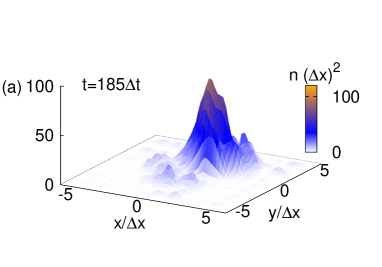
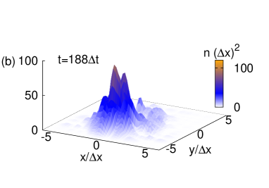
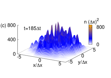
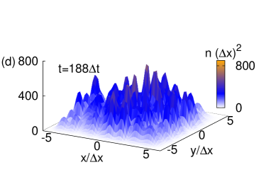
Figure 7: (Color online) Evolution of the condensate dynamics from a traveling soliton (a,b) to a turbulent condensate (c,d) with the increase of the particle creation rate from $R_{0}=0.15\omega_{0}$ to $R_{0}=0.25\omega_{0}$. The eccentricity of the trap is $\varepsilon=0$, time $t$ is shown on the plot.

It was also found that the soliton-like condensate is not formed even for $\epsilon\ll 1$ if the particle creation rate $R_{0}$ is higher than a certain value. In the latter case, a turbulent condensate was observed in the simulations, in agreement with the previous works Refs. Berman et al., 2012a, b. In this turbulent state, a relatively large fluctuating cloud is formed at the center of the trap. The transition from a soliton-shaped to turbulent condensate with the increase of the particle creation rate $R_{0}$ is shown in Fig. 7.

III.4 Comparison of our findings with the existing results

The main object to which our findings can be applied is a non-equilibrium solid-state condensate, e.g. a condensate of excitons, bound electron-hole pairs, in semiconductor heterostructure. Since the lifetime of excitons in a single semiconductor QW is relatively short ($\sim$ a few ns) Feldmann et al. (1987), the experiments with exciton condensates are mostly focused on so-called dipolar (or, indirect) excitons in coupled QWs, where the positively charged holes and negatively charged electrons are located in different QWs, which are separated by a nanometer-wide semiconductor or dielectric barrier Lozovik and Yudson (1975); Negoita et al. (1999); Butov et al. (1994). The dipolar excitons formed by spatially separated charges in coupled QWs are characterized by the relatively long exciton lifetime compared to excitons in a single QW due to small electron-hole recombination rates suppressed by the barrier between QWs. It is worth noting that various experiments have revealed rich collective dynamics of dipolar excitons in coupled QWs and have demonstrated the existence of different phases in an electron-hole bilayer system. The experimental works on excitonic phases in coupled QWs were reviewed in Ref. Butov, 2007. The experimental progress toward probing the ground state of an electron-hole bilayer by low-temperature transport was reviewed in Ref. Das Gupta et al., 2011. The recent progress in the theoretical and experimental developments in the studies of a dipolar exciton condensate in coupled QWs was reviewed in Ref. Snoke, 2013.

Owing to nonzero average electric dipole moment of dipolar excitons, their interactions are long-ranged and decrease with the distance as $\propto r^{-3}$. The presence of the long-range interactions can significantly modify the condensate dynamics under certain regimes Lozovik and Yudson (1978). In particular, in spatially homogenous two-dimensional systems the logarithmic corrections to the chemical potential of the system become essential Lozovik and Yudson (1978). However, it was demonstrated Berman et al. (2012a, b) that under usual experiment conditions for the dipolar exciton condensation in coupled QWs, the most significant contribution to the exciton-exciton dynamics arises from short-range scattering. In effect, the dynamics of the dipolar exciton condensate can effectively be described as the local one, where, however, the effective interaction strength for the condensate particles pairwise interactions is a function of the chemical potential in the system. This quasi-local model has recently been applied to the studied of the nonlinear evolution of dipolar exciton condensates in a radially-symmetric trap Berman et al. (2012a, b).

The observed self-organization of the dipolar exciton condensates may be similar to the dissipative soliton formation known for open nonlinear optical systems, lasers, and chemical systems Akhmediev and Ankiewicz (2005). Solitons dynamics described by one-dimensional conservative Gross-Pitaevskii equation without the source and decay terms (also known as nonlinear Schrödinger equation) was studied in details for the case where the trapping potential is absent (see Refs. Novikov et al., 1984 and Dubrovin et al., 2001 for review). However, in our case, the system is two-dimensional that makes inapplicable the general analytical approaches developed for the integrable one-dimensional nonlinear systems Dubrovin et al. (2001). An extended dimensionality of the systems compared to Refs. Novikov et al., 1984; Dubrovin et al., 2001 results in the presence of additional degrees of freedom, in particular, in the possibility for the soliton to rotate.

It is also worth noting that the soliton propagation has recently been observed in Refs. Amo et al., 2011; Sich et al., 2012; Christmann et al., 2014 for a condensate of polaritons, which are a quantum superposition of the QW excitons and cavity photons Carusotto and Ciuti (2013). In Ref. Amo et al., 2011 the solitons propagate as a perturbation of the steady-state condensate density. In Refs. Sich et al., 2012 and Christmann et al., 2014 the solitons were created by a tightly focused “writing” laser beam and then, freely expanded or traveled in the microcavity. In our case, the exciton condensate spontaneously forms a traveling soliton under spatially homogenous pumping that is, inside the pumping spot. Formation of inhomogeneous polariton condensate patterns have also been considered in Refs. Fernandez et al., 2013 and Christmann et al., 2012. In those works, the inhomogeneities in the condensate density were caused by the interactions of polaritons with a cloud of non-condensed excitons and with structural defects in the cavity. The ring pattern formation was earlier demonstrated for the dipolar excitons in coupled QWs and multiple QWs in previous experimental and theoretical works Butov et al. (2002a); Snoke et al. (2002); Butov et al. (2004); Butov (2007); Fluegel et al. (2011). In spatially resolved measurements, the photoluminescence of the dipolar exciton pattern was seen as a central laser excitation spot surrounded by a sharp ring-shaped region with a diameter much larger than that for the spot and with large dark regions separating the two. In the coupled QWs experiments the voltage was applied perpendicular to the wells, causing the bands to tilt and the electrons and holes to separate. Both the lifetime and the energy of dipolar excitons with spatially separated electrons and holes in different QWs can be tuned by the electric field. The lifetime of quasiparticles in those systems was increased up to microseconds due to the charge separation in different QWs Vörös et al. (2005). In the cases mentioned above the formation of the external rings was caused by the recombination of in-plane spatially separated electrons and holes. The electrically injected carriers created by the external gate voltage recombine with optically injected carriers of the opposite sign Butov et al. (2004); Snoke et al. (2003); Rapaport et al. (2004). In the framework of the microscopic approach formulated in terms of coupled nonlinear equations for the diffusion, thermalization and optical decay of the particles, the formation of the inner ring was explained by the fact that in the optically-pumped area the exciton temperature is much larger than the lattice temperature. As a result, the recombination decay of excitons is suppressed, but while these excitons diffuse out of the optically-pumped area, they cool down and eventually recombine resulting in a local increase of the photoluminescence signal Ivanov et al. (2006). In other words, those experiments did not involve Bose-Einstein condensation of excitons. Formation of the stationary exciton condensate cloud with the size comparable with the size of the laser pumping spot was treated in the framework of the Thomas-Fermi approximation in Refs. Vörös et al., 2006 and Berman et al., 2006. Ring polariton patterns were also excited by an elliptic ring laser spot in experiments Ref. Manni et al., 2011. In contrast to all mentioned cases, the traveling soliton-like condensates reported in this paper have a characteristic size smaller than the excitation spot and are not caused by the kinetics of the free carriers or by the interactions with the structural inhomogeneities. We infer that the soliton formation is caused by the interplay of the Bose-stimulated growth of the condensate that tends to increase the condensate particle density and the exciton-exciton repulsion that leads to the particle spreading in the system.

It is known that the condensation in infinite two-dimensional systems is impossible due to the phase fluctuations that destroy the long-range order in the system Fisher and Hohenberg (1988). To achieve the exciton condensation in quasi-two-dimensional QW structures and to reach high enough exciton densities, at which the system undergoes the BEC transition, most of experiments were conducted with excitons localized in an external trapping potential. A few techniques were utilized to create the exciton traps, including the application of non-uninform mechanical stress to a semiconductor sample Negoita et al. (1999) or electrostatic traps Gartner et al. (2007); High et al. (2012). In these cases, the shape of the exciton trap varied from a radially-symmetric one to a lozenge-shaped, elongated trap Negoita et al. (1999); Gartner et al. (2007).

IV Conclusions

To summarize, a trapped non-equilibrium condensate can exhibit Bose-stimulated self-organization under the conditions where it is driven by a homogenous external sources in a range of frequencies. This self-organization results in formation of spatially-localized structures such as solitary condensate waves – humps or rings. These solitons oscillate in a trap in a manner similar to a classical particle and also can spontaneously rotate. If the asymmetry of the trap exceeds $\varepsilon\geq 0.5$ a conventional fluctuating elongated dipolar exciton cloud is formed instead of a solitary wave. The dynamics of the condensate also depends on the pumping rate. It was found that at increased particle creation rates, the soliton-like condensate dynamics is changed to a turbulent regime. The transition to turbulence at high rates can be attributed to the excitation of multiple interacting degrees of freedom in the system due to nonlinearity. Turbulent exciton condensates have earlier been considered in Refs. Berman et al., 2012a, b.

The spontaneous rotation of the soliton condensate observed in our simulations can be detected in experiments via polarization of the emitted light due to the electron-hole recombination photoluminescence Lagoudakis et al. (2008); Manni et al. (2011). Recently, polarized light has been applied to the multiplexing information transfer through an optical waveguide Barrera et al. (2006); Wang et al. (2012). The future work on the self-organized dipolar exciton condensate might elucidate the ways to control the soliton rotation, to be utilized as a source of coherent polarized light with a given angular momentum $m$. It is of interest for prospective applications in the above-mentioned information technology to investigate how the self-organized condensate reacts on the pulsed or modulated pumping, to create a controllable source of coherent polarized light signals. Self-organized soliton condensate patterns can also potentially be applicable for the information transfer in exciton-based integrated circuits High et al. (2008).