Spectral study on some complex PT-symmetry quantum systems using the Mathews-Lakshmanan position dependent mass in von Roos model and derivation of one parameter kinetic energy [ S.Cruz,J.Negro and L.M.Nieto [Phys.Lett $\bf{369}$(2007)]

Biswanath Rath

$\dagger$ Department of Physics, Maharaja Sriram Chandra Bhanj Deo University, Takatpur, Baripada -757003, Odisha, INDIA

$\dagger$:biswanathrath10@gmail.com

$\bf{Abstract:}$

We investigate the unbroken and broken spectral nature in some position dependent mass related to Mathews-Lakshmanan mass $m(x)=\frac{m_{0}}{(1+(\alpha x)^{2}}$ in complex PT-symmetry potentials with odd term in large$x$ limit using the von Roos model kinetic energy following the suitabitable selection of two parameter condition $2a+b=1$[Cruz,Negro and Nieto:Phys.Lett. $\bf{A369}$(2007)400].In fact the kinetic energy under the condition $b=2a$ becomes $T=-\frac{1}{m^{a}}\partial_{x}\frac{1}{m^{2a}}\partial_{x}\frac{1}{m^{a}}$ a single parameter model, which can be derived using a newly proposed momentum operator called $\bf"pseudo-momentum$(P), where $P=-i\frac{1}{m^{a}}\partial_{x}\frac{1}{m^{a}}$. In fact, the spectra become unbroken in many suitable selection of PT-symmetry i.e $V(x)\sim ix^{2K+1}$ (K=0,1,2).

PACS no-

03.65.Ge,

Key words: von Roos,two parameter condition,pseudo-momentum,unbroken spectra,broken spectra,Mathews-Lakshmanan non singular potential,PT-symmetry

1.Introduction

Since 1983, effective mass model in semiconductor theory($Al_{x}Ga_{1-x}As$) has gained sufficient interest among potential authors to explore new physics coming out of the von Roos model [1,2]on position dependent mass(PDM) Hamiltonian. Considering self-adjoint nature , the Mamiltonian can be written as

$$H=\frac{1}{4}[m(x)^{a}pm(x)^{b}pm(x)^{c}+m(x)^{c}pm(x)^{b}pm(x)^{c}]+V(x)$$ (1)

It is easy to check that

$$H=H^{\dagger}$$ (2)

The classical analogy of the above Hamiltonian is written as

$$h=\frac{p^{2}}{2m(x)}+\zeta x^{2}\rightarrow\zeta=1or1/2$$ (3)

In above the values of a,b,c are constrained subject to the condition $a+b+c=-1$. Some time back Cruz,Negro and Nieto[3] suggested that three parameter model can be reduced to two papameter model provided $a=c$.The prposed model now reduces to

$$H=-\frac{1}{2}[m(x)^{a}\frac{d}{x}m(x)^{2b}\frac{d}{dx}m(x)^{a}+U(x)$$ (4)

with $2a+b=-1$. In this two parameter Hamiltonian ,one can also have large

no of choices. For example (i) $a=\frac{-1}{2};b=0$;(ii)$b=1;a=0$;(iii)

$a=\frac{-1}{\beta}$;$b=\frac{2-\beta}{\beta}$ with suitable choice for

$\beta$. Simple model selected by Cruz ,Negro and Nieto[3] is $\beta=4$. The Hamiltonian used earlier is

$$H_{CNN}=\frac{1}{2}[-\frac{1}{m(x)^{1/4}}\partial_{x}\frac{1}{m^{1/2}}\partial_{x}\frac{1}{m(x)^{1/4}}+V(x)]$$ (5)

In fact authors have systematically selected few cases of singular and non-singular cases of mass. In fact the non-singular case of mass[3]

$$m(x)=\frac{m_{0}=1}{(1+\alpha^{2}x^{2})}$$ (6)

is commonly known as Mathews-Lakshmanan(ML)[4,5] which has been extensively studied classically by many authors. It is quite obvious that as the total Hamiltonian is Hermitian(self-adjoint) in nature, hence the real unbroken spectra is guaranteed[5]. In fact analytical expressions on energy levels have been obtained[3,5]. It is worth mentioning that position-dependent quantum systems still remains an open challenge in complex systems[6]. This motivated me to study the ML mass in complex space. In fact in complex space one of the primary criteria is that the Hamiltonian must be PT-invariant in nature[7]

$$[(PT),H]=0$$ (7)

where

$$PxP^{-1}=-x$$ (8)

$$PpP^{-1}=-p$$ (9)

$$P|x|P^{-1}=|x|$$ (10)

Similarly , the time reversal operator T has the following behaviour

$$TiT^{-1}=-i$$ (11)

$$TpT^{-1}=-p$$ (12)

$$T|p|T^{-1}=|p|$$ (13)

However the term like $ix^{2K+1}$ is PT-symmetric

$$[ix^{2K+1},PT]=ix^{2K+1}$$ (14)

$$[\frac{i}{x^{2K+1}},PT]=\frac{i}{x^{2K+1}}$$ (15)

Similarly, the term like $x^{2}$ satisfies the following

$$[x^{2},P]=0;[x^{2},T]=0;[x^{2},PT]=0$$ (16)

This helps one to construct suitable models in PT-symmetry and study its spectra. In fact it should be borne in mind that PT-symmetry is not the sole criteria for real spectra. It may also exhibit complex spectra partially or fully. However its study using ML type of mass is interesting and will be explored as given below.

$$PxP^{-1}=-x$$ (17)

$$PxP^{-1}=-x$$ (18)

2.Model Kinetic Energy Derivation using ”Pseudo momentum”

Two pameters Kinetic energy

Here we define a new term as ”pseudo momentum ”(P) which is related to momentum (p) as

$$P=\frac{1}{m^{a}}p\frac{1}{m^{b/2}}$$ (19)

Then it is obvious that[8]

$$P\neq P^{\dagger}$$ (20)

then the kinetic energy in this case becomes[9]

$$T=\frac{1}{2}[PP^{\dagger}+P^{\dagger}P]$$ (21)

One parameter Kinetic energy

Here we adopt self-adjoint propertry on $P$ and define as

$$P=\frac{1}{m^{a}}p\frac{1}{m^{a}}$$ (22)

Hence we have

$$P=P^{\dagger}$$ (23)

which is like the standard form of momentum ($p$) ,which is also self-adjoint in its behaviour[8]

$$p=p^{\dagger}$$ (24)

Dimension wise both are different from each other but bearing the same self-adjoint property . The corresponding kinetic energy becomes

$$T=[-\frac{1}{m(x)^{a}}\partial_{x}\frac{1}{m^{2a}}\partial_{x}\frac{1}{m(x)^{a}}]$$ (25)

As the mass appears in denominator of kinetic energy we have $4a=1$,hence $a=\frac{1}{4}$. The corresponding kinetic energy becomes

$$T=[-\frac{1}{m(x)^{1/4}}\partial_{x}\frac{1}{m^{1/2}}\partial_{x}\frac{1}{m(x)^{1/4}}]$$ (26)

It should be remembered that for the K.E of the form

$$T1=\frac{1}{2}[-\frac{1}{m(x)^{1/4}}\partial_{x}\frac{1}{m^{1/2}}\partial_{x}\frac{1}{m(x)^{1/4}}]$$ (27)

The corresponding pseudo momentum can be written as

$$P=\frac{1}{(2m)^{a}}p\frac{1}{(2m)^{a}}$$ (28)

Now using above form of K.E (T) ,we will address the following model complex potentials as given below.

3. Position dependent Hamiltonian in complex space.

At the outset ,we would like to say that all our equations are confined to commutation relation

$$[x,p]=-i[x,\partial_{x}]=-i$$ (29)

so that inerested reader will understand the analysis appropriately. Here we consider mainly two types of model Hamiltonian using the same form of PDM.

case-I

Here the Hamiltonian is of the form

$$H=[-\frac{1}{m(x)^{1/4}}\partial_{x}\frac{1}{m^{1/2}}\partial_{x}\frac{1}{m(x)^{1/4}}+ix^{2K+1}$$ (30)

where$K=0,1,2,...$

(i) K=0 : Broken The corresponding Hamiltonian becomes

$$H^{(1)}=[-\frac{1}{m(x)^{1/4}}\partial_{x}\frac{1}{m^{1/2}}\partial_{x}\frac{1}{m(x)^{1/4}}+ix$$ (31)

(ii) K=1: Unbroken

The corresponding Hamiltonian becomes

$$H^{(2)}=[-\frac{1}{m(x)^{1/4}}\partial_{x}\frac{1}{m^{1/2}}\partial_{x}\frac{1}{m(x)^{1/4}}+ix^{3}$$ (32)

(iii) K=2 : Unbroken

The corresponding Hamiltonian becomes

$$H^{(3)}=[-\frac{1}{m(x)^{1/4}}\partial_{x}\frac{1}{m^{1/2}}\partial_{x}\frac{1}{m(x)^{1/4}}+ix^{5}$$ (33)

(iv) K=3 :Unbroken The corresponding Hamiltonian becomes

$$H^{(4)}=[-\frac{1}{m(x)^{1/4}}\partial_{x}\frac{1}{m^{1/2}}\partial_{x}\frac{1}{m(x)^{1/4}}+ix^{7}$$ (34)

case-II

$$H=[-\frac{1}{m(x)^{1/4}}\partial_{x}\frac{1}{m^{1/2}}\partial_{x}\frac{1}{m(x)^{1/4}}+im(x)x^{2K+1}$$ (35)

(i) K=0 : Broken

The corresponding Hamiltonian becomes

$$H^{(5)}=[-\frac{1}{m(x)^{1/4}}\partial_{x}\frac{1}{m^{1/2}}\partial_{x}\frac{1}{m(x)^{1/4}}+im(x)x$$ (36)

(ii) K=1 : Broken

The corresponding Hamiltonian becomes

$$H^{(6)}=[-\frac{1}{m(x)^{1/4}}\partial_{x}\frac{1}{m^{1/2}}\partial_{x}\frac{1}{m(x)^{1/4}}+im(x)x^{3}$$ (37)

(iii) K=2 : Unbroken

The corresponding Hamiltonian becomes

$$H^{(7)}=[-\frac{1}{m(x)^{1/4}}\partial_{x}\frac{1}{m^{1/2}}\partial_{x}\frac{1}{m(x)^{1/4}}+im(x)x^{5}$$ (38)

(iv) K=3 : Unbroken The corresponding Hamiltonian becomes

$$H^{(8)}=[-\frac{1}{m(x)^{1/4}}\partial_{x}\frac{1}{m^{1/2}}\partial_{x}\frac{1}{m(x)^{1/4}}+im(x)x^{7}$$ (39)

4.Energy calculation method

Here we consider an exactly solvable model ,whose wave functions can be calculated exactly.The model is simple Harmonic Oscillator ,whose Hamiltonian is

$$H_{0}=p^{2}+x^{2}$$ (40)

whose energy eigenvalue satisfy the relation[10]

$$H_{0}|m>=(2m+1)|m>$$ (41)

where

$$|m>=Ne^{-\frac{x^{2}}{2}}H_{m}(x)$$ (42)

In above N stands for normalization constant and $H_{m}(x)$ stands for Hermite polynomial.[8] Here we use matrix diagonalisation method[5] to solve the energy eigenvalue relation

$$H_{p}|\Phi>=E|\Phi>$$ (43)

where $|\Phi>$ is

$$|\Phi>=\sum_{m}A_{m}|m>$$ (44)

As we have introduced a new term i.e ”pseudo-momentum ” we feel to calculate the values of this operator for the ground state i.e

$$<\Phi_{0}|P|\Phi_{0}>$$ (45)

for all the unbroken energy states with a comparison with traditional momentum operator

$$<\Phi_{0}|P|\Phi_{0}>$$ (46)

3. Result and Discussion

Numerical values of energy levels are reflected graphically in figs.1-8. In fact in table-1, we cite the first four energy levels corresponding to unbroken spectra.In table-2 , the values of ” pseudo momentum ” operator have been reflected for the ground state only. Lastly we would like to say that the von Roos[,2] K.E can be derived using the ”pseudo-momentum concept”. In the case of ML oscillator, unbroken energy levels depend on choice of K.

Table-1: First four eigenvalues of position dependent mass Mathews-Lakshmanan mass variation

quantum no	Hamiltonian	Energy levels
0	$H^{(1)}$	1.350 1
1		4.815 1
2		9.415 3
3		14.917 6
0	$H^{(2)}$	1.467 2
1		5.605 9
2		11.8689
3		19.835 8
0	$H^{(3)}$	1.592 2
1		6.224 5
2		13.558 0
3		23.247 9
0	$H^{(7)}$	1.145 5
1		4.282 5
2		9.415 3
3		14.917 6
0	$H^{(8)}$	1.321 0
1		5.120 9
2		11.022 8
3		18.661 6

Table-2:Pseudo-momentum in von Roos model with Mathews-Lakshmanan position dependent mass

quantum no	Hamiltonian	$<\Psi_{0}|P|\Psi_{0}>$
0	$H^{(2)}$	-0.558 0
0	$H^{(3)}$	-0.467 5
0	$H^{(7)}$	-0.579 2
0	$H^{(8)}$	-0.479 7

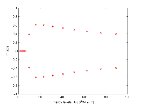
Figure 1: Energy levels of $H=\frac{p^{2}}{M}$ + ix$:PM=\frac{1}{(1+x^{2})}$

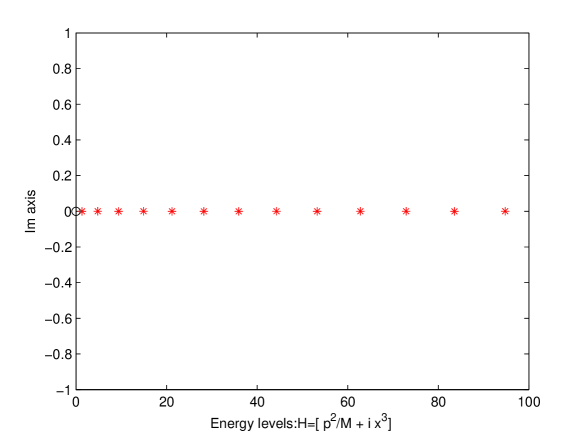
Figure 2: Energy levels of $H=\frac{p^{2}}{M}+ix^{3}:PM=\frac{1}{(1+x^{2})}$

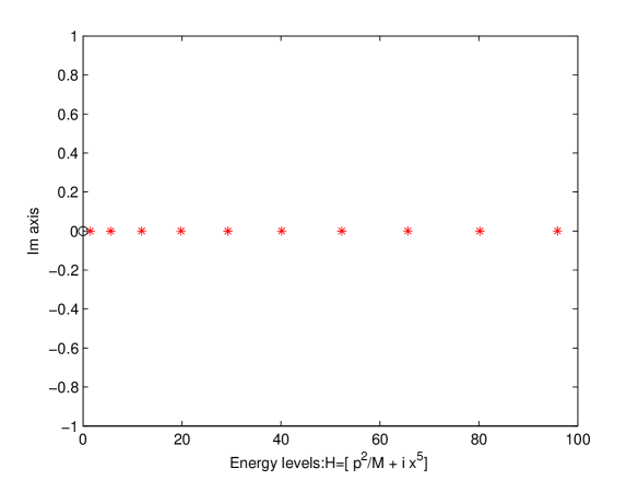
Figure 3: Energy levels of $H=\frac{p^{2}}{M}+ix^{5}:PM=\frac{1}{(1+x^{2})}$

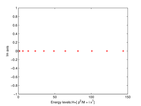
Figure 4: Energy levels of $H=\frac{p^{2}}{M}+ix^{7}:PM=\frac{1}{(1+x^{2})}$

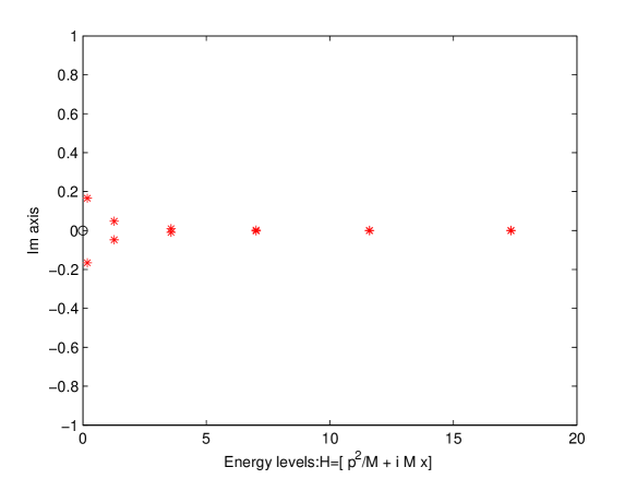
Figure 5: Energy levels of $H=\frac{p^{2}}{M}+Mix:PM=\frac{1}{(1+x^{2})}$

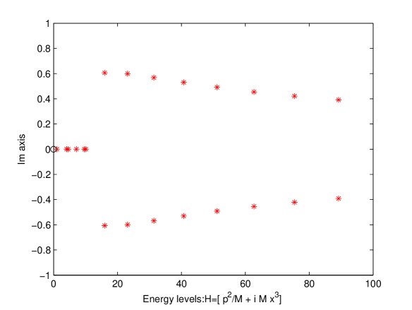
Figure 6: Energy levels of $H=\frac{p^{2}}{M}+iMx^{3}:PM=\frac{1}{(1+x^{2})}$

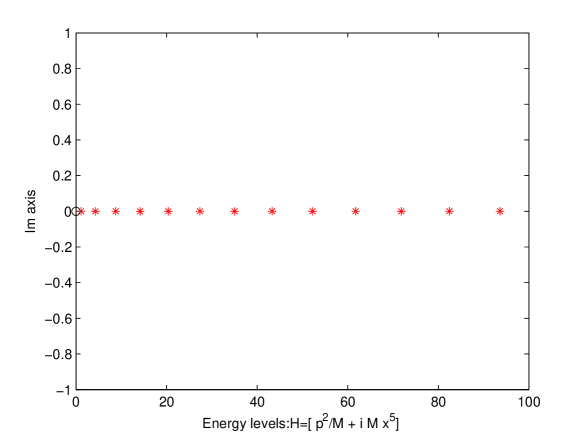
Figure 7: Energy levels of $H=\frac{p^{2}}{M}+iMx^{5}:PM=\frac{1}{(1+x^{2})}$

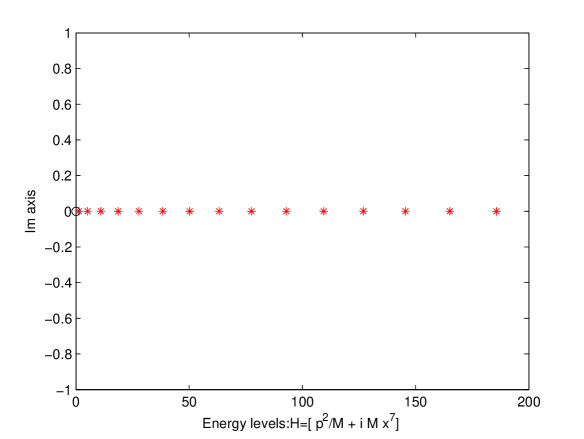
Figure 8: Energy levels of $H=\frac{p^{2}}{M}+iMx^{7}:PM=\frac{1}{(1+x^{2})}$

References

- [1] O.von Roos.Phys.Rev..7547(1983).
- [2] O.von Roos and H.Mavromatis.Phys.Rev..2294(1985).
- [3] S.C.Cruz,J.Negro and L.M.Nieto, Phys.Lett ,400(2007).
- [4] P.M.Mathews and M.Lakshmanan,Quart.Appl.Math,(1974)215.
- [5] B.G.da Costa and E.P.Borges,J.Math.Phys (2018)042101.
- [6] O.Mustafa and S.habib.Mazharimousavi,Phys.Lett (202009)325.
- [7] C.M.Bender,D.C.Brody and H.F.Jones,(2002)270401;(2004) 119902(E);C.M.Bender and H.F.Jones,Phys.Lett (2004) 102.
- [8] A.Yariv”An Introduction to Theory and Applications of quantum mechanics” John Wiley and Sons,New York,(1982);D.J.Graffiths ”Introduction to Quantum Mechanics” Second Edition,Pearson India,(2005);J.L.Powel and B.Crasemann,”Quantum Mechanics” Narosa,India(1988);J.J.Sakurai and J.J.Napolitano,Modern Quantum Mechanics”,Pearson,India(2014);B.H.Bransden and C.J.Joachain,”Quantum Mechanics”,Pearson India(2000);V.Rosansky,Introductory Quantum Mechanics”,Asia Publishing House ,India(1962).
- [9] B.Rath,Phys.Scr (2008)065012;(2010) 069801(Addendum.
- [10] B.Rath and H.Mavromatis.Ind.J.Phys.,641(1999); B.Rath.Eur.Phys.J.Plus .493(2021);B.Rath and P.Mahapatra.Results.in.Phys (2021)104197.