Stellar parameters for stars of the CoRoT exoplanet field

Abstract

Context. Spectroscopic observations represent a fundamental step in the physical characterization of stars and, in particular, in the precise location of stars in the HR diagram. Rotation is also a key parameter, impacting stellar properties and evolution, which modulates the interior and manifests itself on the surface of stars. To date, the lack of analysis based on large samples has prevented our understanding of the real impact of stellar parameters and rotation on the stellar evolution as well as on the behavior of surface abundances. The space missions, CoRoT and Kepler, are providing us with rotation periods for thousands of stars, thus enabling a robust assessment of the behavior of rotation for different populations and evolutionary stages. For these reasons, the follow-up programs are fundamental to increasing the returns of these space missions. An analysis that combines spectroscopic data and rotation/modulation periods obtained from these space missions provides the basis for establishing the evolutionary behavior of the angular momentum of solar-like stars at different evolutionary stages, and the relation of rotation with other relevant physical and chemical parameters.

Aims. To support the computation and evolutionary interpretation of periods associated with the rotational modulation, oscillations, and variability of stars located in the CoRoT fields, we are conducting a spectroscopic survey for stars located in the fields already observed by the satellite. These observations allow us to compute physical and chemical parameters for our stellar sample.

Methods. Using spectroscopic observations obtained with UVES/VLT and Hydra/Blanco, and based on standard analysis techniques, we computed physical and chemical parameters ($T_{\rm{eff}}$ , $\log\,(g)$ , $\rm{[Fe/H]}$ , $v_{\rm{mic}}$ , $v_{\rm{rad}}$ , $v\sin\,(i)$ , and $A(\rm{Li})$ ) for a large sample of CoRoT targets.

Results. We provide physical and chemical parameters for a sample comprised of 138 CoRoT targets. Our analysis shows the stars in our sample are located in different evolutionary stages, ranging from the main sequence to the red giant branch, and range in spectral type from F to K. The physical and chemical properties for the stellar sample are in agreement with typical values reported for FGK stars. However, we report three stars presenting abnormal lithium behavior in the CoRoT fields. These parameters allow us to properly characterize the intrinsic properties of the stars in these fields. Our results reveal important differences in the distributions of metallicity, $T_{\rm eff}$, and evolutionary status for stars belonging to different CoRoT fields, in agreement with results obtained independently from ground-based photometric surveys.

Conclusions. Our spectroscopic catalog, by providing much-needed spectroscopic information for a large sample of CoRoT targets, will be of key importance for the successful accomplishment of several different programs related to the CoRoT mission, thus it will help further boost the scientific return associated with this space mission.

1 Introduction

The CoRoT (Convection, Rotation, and planetary Transits) space mission (Baglin et al., 2007) collected a total of 161,303 point-source photometric data over a period of six years for stars exhibiting different luminosity classes and spectral types. This space mission had two main goals: 1) the detection of extra-solar planets using the transit procedure, and 2) precise stellar seismology. In addition to these two big challenges, other programs related to the CoRoT mission are helping further our understanding of a variety of important astrophysical phenomena, such as stellar activity, pulsation, and multiplicity. In this context, CoRoT provides a unique opportunity for the study of stellar rotation, which is recognized as a fundamental quantity that controls the evolution of stars, however, it is only today that the models and observations in hand to begin to address it. In this sense, CoRoT offers the necessary tools for the photometric measurements of rotation periods for a statistically robust sample of stars at different evolutionary stages and belonging to different stellar populations.

However, in spite of the large amount of high-quality photometric data obtained with CoRoT, ground-based observations are also needed to accomplish the main scientific goals of the mission. For this reason, several observational programs have increased the photometric database related to the CoRoT mission (e.g., Aigrain et al., 2009; Deleuil et al., 2009). These data enabled the establishment of the best fields and observation setups to observe with the satellite, also establishing the spectral types and luminosity classes for the stars in the CoRoT fields. Nevertheless, important uncertainties are still present in these classifications because of the variable reddening levels affecting the CoRoT fields, in addition to the still unknown chemical abundances and distances to the targets.

Spectroscopic observations are mandatory for a solid treatment of the different CoRoT scientific goals. In this sense, two large spectroscopic surveys of CoRoT targets have been carried out to date, both using multifiber observations. The first survey (Gazzano et al., 2010, G10 hereafter) combined multifiber observations with an automated procedure for the determinations of different stellar parameters, whereas the second was dedicated essentially to spectral classification (Sebastian et al., 2012).

In the context of the physical characterization of CoRoT targets, we carried out a large spectroscopic survey focused on the brightest F-, G-, and K-type stars in the CoRoT exoplanetary fields LRc01 and LRa01, using the multifiber spectrographs UVES/VLT and Hydra/Blanco, with high and medium spectral resolution, respectively. Using these observations, we applied a homogeneous procedure for the determination of different stellar parameters, including effective temperature ($T_{\rm{eff}}$ ), surface gravity ($\log\,(g)$ ), overall metallicity ($\rm{[Fe/H]}$ ), radial velocity ($v_{\rm{rad}}$ ), projected rotational velocity ($v\sin\,(i)$ ), and microturbulence ($v_{\rm{mic}}$ ). The main goal of this paper is to present the corresponding catalog. We also present the mean values for stellar parameters of the two stellar populations in the CoRoT anticenter/center direction. The paper is structured as follows: in Sect. 2 we describe the observations and data reduction. Sect. 3 describes how we derived the stellar parameters for the stars in our sample, and Sect. 4 contains our main results. Finally, we draw our conclusions in Sect. 5.

2 Observations

The present stellar sample is composed of 138 stars of spectral types F, G, and K, with visual magnitudes $V$ between $10$ to $14$, located in two exoplanet fields observed by CoRoT, namely the Galactic center ($\rm{LRc}01$: Long Run Center 01) and the Galactic anticenter ($\rm{LRa}01$: Long Run Anticenter 01) fields. We selected the sample using as criteria the visual magnitude V, the spectral type, and the luminosity classes defined by Deleuil et al. (2009) for CoRoT targets. We selected stars belonging to luminosity classes II, III, IV, and V considering the range in V and spectral type defined above. Our sample is comprised of the brightest stars in both CoRoT fields, and is thus not fully representative of the magnitude and color distribution of CoRoT stars.

To obtain a physical characterization for these stars, a series of spectroscopic observations were carried out using two spectrographs. A sample of $53$ stars was observed using the high-resolution UVES spectrograph (hereafter UVES stars ) mounted on the Kuyen/VLT 8.2m telescope, located in Cerro Paranal, Chile, in the course of different observing runs in 2006. The UVES standard setup DICH-2 ($390-760$nm) with a $0.9$ arcsec slit was used, allowing us to obtain high-resolution ($R\approx 47,\!000$) and high signal-to-noise ($S/N>100$) spectra.The main characteristics of the targets and the observation dates are given in Table LABEL:TAB:FUVES.

A complementary sample of $85$ stars was observed using the Hydra multifiber echelle spectrograph (henceforth Hydra stars ), mounted on the Blanco 4m telescope at the Cerro Tololo Interamerican Observatory, located in Cerro Tololo, Chile. The filters $E5187$ ($509-525\leavevmode\nobreak\ nm$) and $E6757$ ($656-681$ nm) with a $200$ micron slit were used, allowing us to collect spectra with medium resolution ($R\approx 17,\!000$ and $15,\!000$, respectively) and signal-to-noise ratio $70<S/N<200$. The $E5187$ filter was chosen because it covers a spectral region with five Fe II lines, whereas the $E6757$ was chosen because several Fe I lines and a Li doublet (at $\approx 671\,{\rm nm}$) are located in spectral window. Also, a few stars, with accurate previous measurements of $v\sin\,(i)$ and with FGK spectral types, were also observed with the same Hydra setups (Melo et al., 2001) to construct a calibration for the determination of $v\sin\,(i)$ for the Hydra stars in our sample. Figure 1 shows examples of these observations using both instruments.

Table 2 shows the setup used in Hydra observations. For the targets, we also compiled luminosity classes, $V$-band magnitudes, and color indices from the CoRoT database, as well as $JHKs$ magnitudes from the Two-Micron All-Sky Survey (2MASS) database (Skrutskie et al., 1996). The main characteristics of the targets and the observation dates, and corresponding luminosity classes (from the CoRoT and 2MASS databases) are given in Tables LABEL:TAB:FHYDRA and 4.

Figure 1: Some spectra of the stars contained in the sample. Spectra collected using the UVES spectrograph are show in the upper panel, whereas the lower panel shows spectra collected using the Hydra spectrograph.

The reduction of UVES stars data was done using the standard UVES data reduction pipeline (Ballester et al., 2000). Hydra data were reduced using the dohydra task in IRAF. Both reductions follow the usual reduction steps (bias, flat-field, and background corrections, fiber order definition, wavelength calibration of the spectra with Th-Ar lamp spectra, and extraction of the spectra). Then we use IRAF to normalize the spectra to a pseudocontinuum level and to bring the reduced spectra to the rest frame. Cosmic rays were extracted using the procedures described in van Dokkum (2001).

3 Stellar properties

3.1 Radial velocities $v_{\rm{rad}}$ 

We obtained radial velocities $v_{\rm{rad}}$ with the fxcor task (Tonry & Davis, 1979) in IRAF. Because the stars of the UVES sample present $T_{\rm{eff}}$ close to the solar value, we cross-correlated the UVES spectra with a spectrum of the Sun (Hinkle et al., 2000). We then converted the shifts into radial velocities of the stars, and we applied a barycentric correction. On the other hand, because the Hydra stars present a greater spread in temperatures and luminosity classes, the spectra were cross-correlated with synthetic spectra of the Sun and an RGB star ($T_{\rm{eff}}$ $=4000$ K, $\log\,(g)$ $=1.0$ dex and $\rm{[Fe/H]}$ $=0.0$ dex) to compare differences in the determinations of radial velocities. We computed the spectra with the Turbospectrum code (Alvarez & Plez, 1998) and MARCS atmosphere models with solar abundances (Gustafsson et al., 2008). In Fig. 2 small differences can be found between the radial velocities derived using the synthetic spectra (averaging about $-0.27\pm 0.37$  ${\rm km\,s}^{-1}$ ). We opted to use the values found using the synthetic solar spectrum, and applied a barycentric correction. The typical errors in radial velocities for Hydra stars are lower than $0.5$  ${\rm km\,s}^{-1}$ . On the other hand, we also computed a synthetic solar spectrum for the UVES spectral resolution, which we used to obtain $v_{\rm{rad}}$ for the UVES sample, to find systematic errors in the Hydra $v_{\rm{rad}}$ measured using synthetic spectra. We found that our measurements of $v_{\rm{rad}}$ using synthetic spectra present a systematic difference of about $-0.75\pm 1.66$  ${\rm km\,s}^{-1}$ with those derived with observed solar spectrum, and is thus not significant.

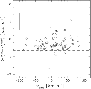
Figure 2: Comparison between the $v_{\rm{rad}}$ measurements for the Hydra sample obtained using different synthetic spectra. The $v_{\rm{rad}}^{RGB}-v_{\rm{rad}}^{Solar}$ represents the difference between the $v_{\rm{rad}}$ obtained when the Hydra spectra are cross-correlated with synthetic spectra for a RGB star and the Sun, respectively. The red line represents the mean value of $v_{\rm{rad}}^{RGB}-v_{\rm{rad}}^{Solar}$ and its the standard deviation is presented using black dashed lines. Also, the typical error in $v_{\rm{rad}}$ measurements for Hydra stars is shown using an error bar.

3.2 Rotation velocities $v\sin\,(i)$ 

The $v\sin\,(i)$ measurements of our targets were computed using two procedures. For the case of UVES stars , the $v\sin\,(i)$ values were determined using the same procedure as in Canto Martins et al. (2011). Following these authors, the resulting spectra (taking into account the instrumental profile of UVES) are convolved with rotational profiles to adjust the broadening observed in the iron lines (profile fitting) located between $6700$ and $6715$ Å.

The $v\sin\,(i)$ values for the Hydra stars were computed (using the fxcor task) with a cross-correlation function (CCF) especially calibrated for the Hydra spectrograph. We then followed the same procedure decribed before for the . As is described in Recio-Blanco et al. (2002) and Lucatello & Gratton (2003), the relation between $v\sin\,(i)$ and the corrected width $\sigma_{obs0}$ of the CCF is

$$v\sin\,(i)\,=A\sqrt{(\sigma_{obs0})^{2}-(\sigma_{0})^{2}}\leavevmode\nobreak\ \leavevmode\nobreak\ \rm{km\leavevmode\nobreak\ s^{-1}},$$ (1)

where $A$ and $\sigma_{0}$ are the so-called coupling constant and the nonrotational contribution to the CCF width, respectively. As mentioned in Melo et al. (2001), $\sigma_{0}$ depends on different broadening mechanisms (magnetic field, instrumental profile, thermal broadening, etc.), which is related to object star and the template used, but does not depend on rotation.

Since the setup $E5187$ presents the highest resolution in our Hydra observations, it was chosen to determine the $v\sin\,(i)$ values. We used FGK stars with reliable $v\sin\,(i)$ determinations as templates and calibrators, which were observed during our observing runs. The $v\sin\,(i)$ values and photometry for these stars are compiled in Table 4.

The fxcor task allowed us to obtain the uncorrected width of the CCF ($\sigma_{obs}$), which has a contribution from the template used ($\sigma_{t}$) in deriving the CCF. The $\sigma_{t}$ can be determined with an autocorrelation for each template, as is described in equation 4 of Lucatello & Gratton (2003). For each star used as template we obtained several spectra, which allowed us to avoid the autocorrelation of the same spectrum. The $\sigma_{obs}$ and $\sigma_{t}$ are related with the corrected width $\sigma_{obs0}$ through the following equation:

$$(\sigma_{obs0})^{2}=(\sigma_{obs})^{2}-(\sigma_{t})^{2}.$$ (2)

The mean values of $\sigma_{obs}$ and $\sigma_{t}$ for each template are listed in Table 5, whereas the mean values of $\sigma_{obs}$ for each calibrator star are listed in Table 6. Finally, using a linear fit in the plane $[(\sigma_{obs0})^{2},(v\sin(i))^{2}]$ the following relation between $v\sin\,(i)$ and $\sigma_{obs0}$ was obtained:

$$v\sin(i)=(0.861\pm 0.017)\sqrt{\sigma_{obs0}^{2}-(21.404\pm 0.835)^{2}}\leavevmode\nobreak\ \leavevmode\nobreak\ \rm{km\leavevmode\nobreak\ s^{-1}}.$$

The errors in these coefficients are associated with the errors in the slopes of the linear fit. In Fig. 3 we show the final calibration, which presents a good agreement with the reference values of $v\sin\,(i)$ for calibrator stars.

Figure 3: The CCF-$v\sin\,(i)$ calibration for the Hydra spectrograph. The dashed line represents the function found and black points represent the values for the calibrator stars, respectively.

These $v\sin\,(i)$ values were used as reference to obtain new measurements of $v\sin\,(i)$ values using the setup $E6757$ and the same method described for UVES stars . Note that the setup $E6757$ contains the spectral region between $6700$ and $6715$ Å. Small differences were found between $v\sin\,(i)$ values derived using both methods. Since we use the profile fitting to derive lithium abundances (as is described in section 4.4), the final values of $v\sin\,(i)$ for the Hydra stars are those derived from the profile fitting.

3.3 Effective temperatures $T_{\rm{eff}}$ , surface gravities $\log\,(g)$ , iron abundance $\rm{[Fe/H]}$ , and microturbulence velocity $v_{\rm{mic}}$ 

Because our stellar sample is comprised of stars belonging to the field, it is important to have an estimation of their stellar parameters, which were used to avoid mistakes in the determination of the final parameters. In this sense, as a first step in the derivation of atmospheric parameters, we used the 2MASS $JHK$ near-infrared photometry and the CoRoT database mean values of $\langle V\rangle$ and $\langle(B-V)\rangle$ to obtain a first estimation of the effective temperature for our sample. Specifically, we used the mean CoRoT color index $(B-V)$ and the calibrations of Flower (1996) corrected by Torres (2010) to calculate the photometric effective temperature $T_{\rm{eff}}(B-V)$. In the same way, we calculated the photometric effective temperature $T_{\rm{eff}}(J-K)$ using the 2MASS color index $(J-K)$, the CoRoT luminosity classes, and the calibrations of Alonso et al. (1996, 1999). We derived these temperatures without reddening corrections (see section 4.3 for detailed discussion). Also, we found errors at levels of $0.04$ mag in the $(J-K)$ for the stars in our sample, which implies errors at levels of $130$ K in $T_{\rm{eff}}(J-K)$. No errors are informed in the CoRoT database for $(B-V)$.

We used the average between both photometric temperatures as our initial estimation for the spectroscopic temperature. At the same time, we estimated the initial values of surface gravities $\log\,(g)$ using the CoRoT luminosity classes and interpolations in tables of infrared synthetic colors computed with ATLAS9 by R. Kurucz. These initial estimates can present important errors, produced by reddening and bad identification of CoRoT luminosity classes (see Fig. 8 in G10). In fact we found differences of about $>500$ K between photometric and spectroscopic temperatures, which implies high rates of extinction in the CoRoT fields (see Section 4.3). For this reason we stress that these initial values were used only as a starting point to obtain the final parameters and, in any case, they constrained the searching of spectroscopic temperatures.

We determined final values of the atmospheric parameters and their respective errors using the Turbospectrum code and MARCS atmosphere models with solar abundances. Solar abundances were taken from Asplund et al. (2005), and the collisional damping treatment was performed based on the work of Barklem and co-workers (Barklem et al., 2000a, b; Barklem & Piskunov, 2003; Barklem & Aspelund-Johansson, 2005). To compute synthetic spectra with the Turbospectrum code, we took atomic (see below) and molecular line lists into account, including TiO (Plez, 1998), VO (Alvarez & Plez, 1998), and CN and CH (Hill et al., 2002). The Turbospectrum code uses equivalent widths ($EW$) to compute abundances $A(\rm{Fe})$ corresponding to the different Fe lines. The list of Fe lines used was compiled and corrected by Canto Martins et al. (2011) (see their Table 6). This list is composed of $91$ and $14$ lines of Fe I and II, respectively. There are differences in the number of iron lines used to characterize the stars because our sample was observed using two instruments and different setups. In particular, for UVES stars, we used all lines compiled by Canto Martins et al. (2011), whereas for the Hydra stars $33$ of the lines ($28$ FeI lines and $5$ FeII lines) in the intervals $5090-5250$ Å  and $6560-6810$ Å  were used. We measured $EW$ values with the DAOSPEC code (Stetson & Pancino, 2008). Using excitation equilibrium for the FeI abundances, FeI/FeII ionization equilibrium, and the equilibrium of the $A(\rm{Fe})$ values and their respective $EW$ values, we can derive effective temperatures $T_{\rm{eff}}$ , surface gravities $\log\,(g)$ , and microturbulence velocities $v_{\rm{mic}}$ , respectively. Starting from the photometric parameters, we ran the Turbospectrum code iteratively using MARCS atmosphere models with different parameters to find the three equilibria, thus defining the final parameters. Figure 4 presents an example of physical and chemical parameter determinations using the equilibria (slopes equal to zero in the planes shown in this figure) for both a UVES star and a Hydra star.

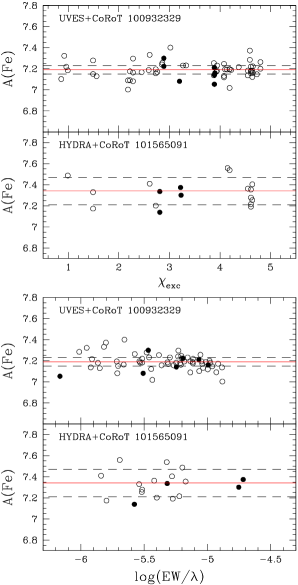
Figure 4: Upper panels: ionization equilibrium for the targets $100932329$ (UVES star) and $101565091$ (Hydra star). Lower panels: equilibrium of the $A(\rm{Fe})$s and their $EW$s. Open and filled circles represent the abundances of FeI ($A(\rm{FeI})$) and FeII ($A(\rm{FeII})$), respectively. Red and black dashed lines represent the mean value of $A(\rm{Fe})$ and standard deviation, respectively.

The errors in $T_{\rm{eff}}$ and $v_{\rm{mic}}$ are obtained from the errors in the slopes that define the equilibria described above. We change one of these parameters, keeping the others fixed, and compute a new atmospheric model. We found the error when the slope of the new fit became equal to its respective slope error. The error in $\rm{[Fe/H]}$ is equal to slope error in excitation equilibrium for the FeI abundance. Finally, the error in $\log\,(g)$ is found when the difference between $A(\rm{FeI})$ and $A(\rm{FeII})$ is equal to the square root of the sum of the squares of the errors in $A(\rm{FeI})$ and $A(\rm{FeII})$.

3.4 The Li abundance determinations

The $\rm{Li}$ abundances $A(\rm{Li})$  for UVES and Hydra stars were calculated by fitting the observed profile with a synthetic profile of the $\rm{Li}$ doublet located at $\sim 6708$ Å. The synthetic spectrum was computed using the Turbospectrum code. Figure 5 shows four examples showing the method used to determine the $A(\rm{Li})$.

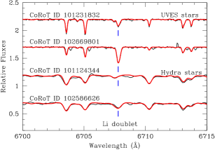
Figure 5: The profile fitting of the Li doublet at $\sim 6708$ Å  is shown for two UVES stars (CoRoT ID $101231832$ and $102669801$) and two Hydra stars (CoRoT ID $101124344$ and $102586626$). The observed spectra are presented using black lines, whereas the synthetic spectra are shown in red. The position of the Li doublet is indicated with a blue vertical line.

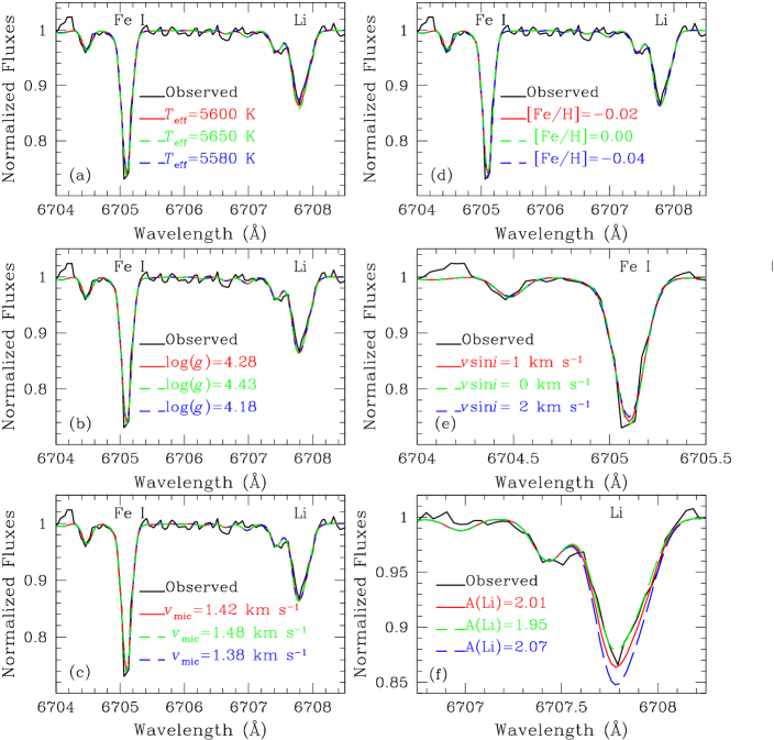
Figure 6: As in Fig. 5, for the CoRoT ID $101231832$ the profile fitting of an Fe I line and the Li doublet are presented. The panels (a), (b), (c), and (d) show how the errors in each stellar parameter impact the computed synthetic spectra, which were used to measure $v\sin\,(i)$ (panel e) and $A(\rm{Li})$ (panel f), and their respetive errors. For all panels, the observed spectrum is presented using a black line, whereas the synthetic spectrum, computed with the derived stellar parameters, is presented using a red line. The dashed green and blue lines represent the computed synthetic spectra with errors for a given stellar parameter.

The error $\sigma_{A({\rm Li})}$ in this abundance is related to the errors in the physical and chemical parameters; more specifically, the magnitude of this error is directly related to the error in $T_{\rm{eff}}$ , and the errors in the other stellar parameters, such as $\log\,(g)$ , $v_{\rm{mic}}$ , and $v\sin\,(i)$ , produce minor effects in the measurements of $A({\rm Li})$. We determined new lithium abundances using synthetic spectra reflecting the errors in the four stellar parameters described above, which we called $A(\rm{Li})^{j}_{ER}$. Then, the final error $\sigma_{A({\rm Li})}$ is equal to the square root of the sum of the squares of the difference between $A(\rm{Li})$ and $A(\rm{Li})^{j}_{ER}$, as is described in the following equation:

$$\sigma_{A({\rm Li})}=\sqrt{\sum_{\rm{j=1}}^{\rm{j=4}}\left(A({\rm Li})-A(\rm{Li})^{j}_{ER}\right)^{2}}.$$ (3)

The Fig. 6 shows how the errors in the stellar parameters impact in the $A({\rm Li})$. In this context, the measurements of $A({\rm Li})$ for Hydra stars present errors higher than those found for the . Nevertheless, we should be cautious with the Hydra data due, in particular, to the spectral resolution ($R\sim 15,\!000$) associated with the observations.

4 Results

The computed stellar parameters, including rotational velocities $v\sin\,(i)$ and lithium abundances, for the present stellar sample are listed in Table LABEL:TAB:ALLPARAMETERS. Figure 7 presents the corresponding Hertzsprung-Russell (HR) diagram, with the stars segregated by their Galactic locations (CoRoT center/anticenter) and iron abundances. In the bottom panel, stars are divided in three different groups using their $\rm{[Fe/H]}$ values. Errors in the parameters are also included in these panels. The magnitude of these errors is linked to the quality of the spectra, including spectral resolution $R$ and $S/N$, and intrinsic effects of the stellar surfaces (i.e., high $v\sin\,(i)$ , molecular bands in cool stars, etc.). Figure 7 shows that the present sample is comprised of stars in different evolutionary stages, ranging from the main sequence (MS) to the red giant branch (RGB).

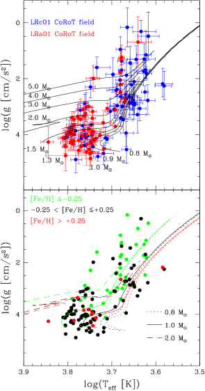
Figure 7: Upper panel: HR diagram of the stellar sample segregated by Galactic direction (center/anticenter). Blue and red dots represent stars in the $\rm{LRc}01$ and $\rm{LRa}01$ fields, respectively. Evolutionary tracks for $Z=0.019$, from Girardi et al. (2000), are shown for stellar masses between 0.8 and 5 M_⊙. Lower panel: HR diagram of the stellar sample segregated by the iron abundance $\rm{[Fe/H]}$. Green, black, and red points represent stars with $\rm{[Fe/H]}$ $\leq-0.25$, $-0.25<$$\rm{[Fe/H]}$ $\leq+0.25$ and $\rm{[Fe/H]}$ $\geq+0.25$, respectively. Evolutionary tracks for $Z=0.004$, $Z=0.019$, and $Z=0.030$, from Girardi et al. (2000), are presented with lines in green, black, and red, respectively. In this panel, only the following stellar mass values are represented: $0.8\leavevmode\nobreak\ M_{\odot}$ (dot lines), $1.0\leavevmode\nobreak\ M_{\odot}$ (solid lines) and $2.0\leavevmode\nobreak\ M_{\odot}$ (dash lines). For clarity, in both panels we plot only the evolutionary tracks until to the RGB stage.

We used the evolutionary tracks of Girardi et al. (2000) for different masses and metallicities to identify the evolutionary stages of the stars in our sample. For this purpose, we identified the turn-off and the base of the RGB from the evolutionary tracks for each $Z$ to define the MS, subgiant branch (SGB), and RGB regions. The results of this classification are listed in Table LABEL:TAB:ALLPARAMETERS. Mean values for the stellar parameters and their respectives standard deviations corresponding to different CoRoT fields and evolutionary stages are given in Table 8.

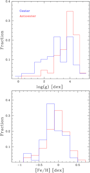
Figure 8: Upper panel: histogram of the surface gravities $\log\,(g)$ in the CoRoT fields. Lower panel: histograms of the iron abundances $\rm{[Fe/H]}$ for the different evolutionary stages. A relation between $\rm{[Fe/H]}$ and evolutionary status is clearly present for the stars in our sample.

Figure 7 also shows that the stellar evolutionary distribution for LRc01 and LRa01 CoRoT fields agrees with Deleuil et al. (2009). Furthermore, the relation between the color and evolutionary status is linked to the stellar metallicity. In fact, as we can see in Fig. 8 and Table 8, the distributions of $\log\,(g)$ for both fields are different and these differences correlate with the $\rm{[Fe/H]}$ distributions. Most $\rm{LRa}01$stars have $\log\,(g)$ $\geq 3.75$ dex ($\sim 64\%$), whereas the $\rm{LRc}01$stars are spread along a large interval of $\log\,(g)$ and most of them have $\log\,(g)$ $\leq 3.75$ dex. Combining this with the fact that the peaks of the $\rm{[Fe/H]}$ distributions and their mean values (Table  8) are different from one another, we can see that there is a relation between temperature, surface gravity, and evolutionary stage in the CoRoT fields considered here. While one might be tempted to associate these differences to selection effects, we note that these results agree with the recent spectroscopic survey of the CoRoT fields presented by G10. This point is discussed further in Sec. 4.4.

4.1 Comparison with previous results

To verify our results, we compared them with the results presented in G10. Only 11 stars of our sample were also analyzed by G10. These stars are listed in Table 9. In Fig. 9 we plot the comparison between our results and the G10 findings. Our results agree with the survey of G10, with $T_{\rm{eff}}$ , $\log\,(g)$ and $v\sin\,(i)$ presenting only small differences for most of the stars. However, star $101538522$ presents a large dispersion in the $\log\,(g)$ values, which may be explained because of the quality of the data of G10 for a RGB star ($S/N\sim 23$). We cannot directly compare their derived abundances with ours since G10 report only the global metallicity ($\rm{[M/H]}$), whereas here we present the iron abundance ($\rm{[Fe/H]}$ ).

Figure 9: Comparison between our results and the results of G10 for stars in common. Some differences can be noted, however, overall our result agree with G10.

4.2 Radial and rotational velocities

Figure 10 shows the distribution of the measurements of barycentric radial velocity $v_{\rm{rad}}$ and rotational velocity $v\sin\,(i)$ listed in Tables LABEL:TAB:ALLPARAMETERS and 8. Small, but significant, differences are observed in the $v_{\rm{rad}}$ distribution for stars located in the Galactic center and anticenter directions. The percentages of stars with $v_{\rm{rad}}$ $\leq 0$  ${\rm km\,s}^{-1}$ associated with the Galactic center and anticenter directions are $64\leavevmode\nobreak\ \%$ and $50\leavevmode\nobreak\ \%$, respectively. In spite of the incompleteness of the sample, this behavior agrees with the $v_{\rm{rad}}$ distribution determined by G10 (see their Fig. 2).

In Fig. 10, small differences are also observed in the distribution of $v\sin\,(i)$ values. In fact, $68\leavevmode\nobreak\ \%$ and $42\leavevmode\nobreak\ \%$ of stars in the $\rm{LRc}01$and $\rm{LRa}01$fields present $v\sin\,(i)$ $\leq 5$  ${\rm km\,s}^{-1}$ , respectively. The difference disapears quickly for stars with $v\sin\,(i)$ $\leq 10$  ${\rm km\,s}^{-1}$ , where the percentage for both fields are similar ($89\leavevmode\nobreak\ \%$ and $83\leavevmode\nobreak\ \%$ for $\rm{LRc}01$and $\rm{LRa}01$fields, respectively). A few high rotation values can be noticed among stars in the Galactic center region While we caution that these distributions are affected to some degree by incompleteness, the observed behavior of the $v\sin\,(i)$ distribution in particular does follow the behavior expected for FGK stars (Soderblom, 1983; de Medeiros et al., 1996; Nordström et al., 2004). In fact, as we can see from Figure 11, which displays the individual $v\sin\,(i)$   values versus $T_{\rm{eff}}$ , the rotational behavior for stars of the present stellar sample is rather well in agreement with the well-established behavior of rotation for stars evolving from the MS to red giant stages. Essentially, stars in the MS exhibit a wide range of rotational velocity values, which are related with the stellar masses and $T_{\rm{eff}}$ . For these stars, the measured values of $v\sin\,(i)$ ranges from a few km/s to about 100 times the solar rotation rate, whereas the stars along the RGB are typically slow rotators, except for a few unusual cases presenting moderate to rapid rotation (Cortés et al., 2009; Carney et al., 2008, 2003; de Medeiros et al., 1996; de Medeiros & Mayor, 1990).

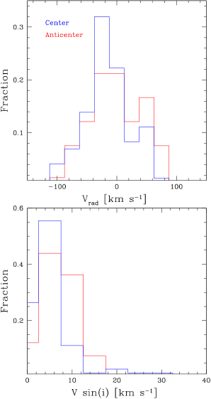
Figure 10: Upper panel: histograms of the radial velocity $v_{\rm{rad}}$ for the $\rm{LRc}01$ (blue line) and $\rm{LRa}01$ (red line) fields. Lower panel: histograms of the rotational velocity $v\sin\,(i)$ for the $\rm{LRc}01$ (blue line) and $\rm{LRa}01$ (red line) fields.

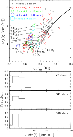
Figure 11: Upper panel: distribution of $v\sin\,(i)$ for the stars in our sample along the HR diagram. Symbol size is proportional to the $v\sin\,(i)$ value. Evolutionary tracks are defined as in Fig. 7. Lower panels: histograms of the rotational velocity $v\sin\,(i)$ for the different evolutionary stages.

4.3 Photometric temperatures and reddening

It is possible to evaluate the reddening effects along the two different Galactic directions by comparing the initial photometric temperatures, derived without taking reddening into account, and the final, spectroscopically-derived, and presumably reddening-insensitive temperatures. This analysis allows one to establish how the determination of physical parameters from photometric data is affected by neglecting reddening effects, to evaluate the error budget brought about by reddening, and also to check the presence of possible reddening gradients in the CoRoT windows. In this sense, the present $E(B-V)$ estimates for individual stars may assist follow-up programs of specific groups of stars, including for instance solar analogs and solar twins.

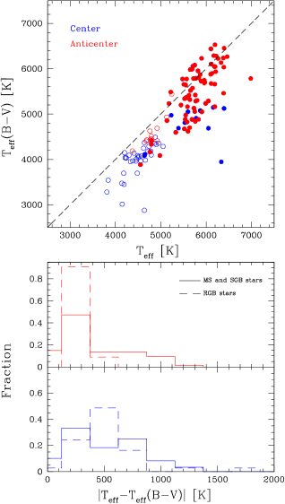
Figure 12: Upper panel: differences between photometric $T_{\rm{eff}}(B-V)$ and spectroscopic $T_{\rm{eff}}$ for stars in the $\rm{LRc}01$ (open and filled blue dots) and $\rm{LRa}01$ (filled and open red dots) CoRoT fields. Filled circles represent MS and SGB stars, whereas open circles represent RGB stars. Lower panels: histograms of the difference between photometric $T_{\rm{eff}}(B-V)$ and spectroscopic $T_{\rm{eff}}$ for the stars in the $\rm{LRc}01$ (blue line) and $\rm{LRa}01$ (red line) CoRoT fields.

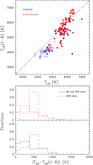
Figure 13: Upper panel: differences between photometric $T_{\rm{eff}}(J-K)$ and spectroscopic $T_{\rm{eff}}$ for the stars in the $\rm{LRc}01$ (open and filled blue dots) and $\rm{LRa}01$ (filled and open red dots) CoRoT fields. Filled circles represent MS and SGB stars, whereas open circles represent RGB stars. Lower panels: histograms of the difference between photometric $T_{\rm{eff}}(J-K)$ and spectroscopic $T_{\rm{eff}}$ for the stars in the $\rm{LRc}01$ (blue line) and $\rm{LRa}01$ (red line) CoRoT fields.

To accomplish this goal, we compare the photometric temperatures $T_{\rm{eff}}(B-V)$ and $T_{\rm{eff}}(J-K)$ and those derived from our spectroscopic analysis, $T_{\rm{eff}}$. We determined the photometric temperatures, at the beginning, using the luminosity class from the CoRoTSky database. For some stars, however, the physical parameters provide a new classification of luminosity class for which new photometric temperatures were computed using this information. The photometric temperatures are listed in Table LABEL:TAB:ALLPARAMETERS, including those derived using a new luminosity class. Finally, in Figs. 12 and 13, we present the comparisons between our spectroscopic $T_{\rm{eff}}$ values and the photometric estimations $T_{\rm{eff}}(B-V)$ and $T_{\rm{eff}}(J-K)$.

Figure 12 shows that the stars in CoRoT run $\rm{LRc}01$ present larger differences between $T_{\rm{eff}}(B-V)$ and $T_{\rm{eff}}$ than those in run $\rm{LRa}01$, which can be expected because of the higher extinction levels in the Galactic center direction. In fact, for this color index, (B–V), the percentages of CoRoT stars presenting differences up to $200$, $500$, and $800$ K in the Galactic center direction are $6\leavevmode\nobreak\ \%$, $42\leavevmode\nobreak\ \%$, and $81\leavevmode\nobreak\ \%$, respectively. The percentages of CoRoT stars presenting the same temperature differences in the Galactic anticenter direction are $38\leavevmode\nobreak\ \%$, $86\leavevmode\nobreak\ \%$, and $92\leavevmode\nobreak\ \%$, respectively. To obtain a reddening estimation for the LRc01 and LRa01 CoRoT fields, we used the calibration of Flower (1996)(corrected by Torres 2010), which give us $T_{\rm{eff}}(B-V)$ and $T_{\rm{eff}}$ , assuming the latter (spectroscopically derived) as being the actual value. This assumption is valid because $T_{\rm{eff}}$ is not affected by reddening. As such, for a star with a solar value $(B-V)_{\odot}$, we estimated reddening levels ($E(B-V)$) of about $0.06$, $0.17$, and $0.30$, for the differences of $200$, $500$, and $800$ K, respectively. Similarly, for an RGB star with a $(B-V)_{0}\sim 1.6$, these differences in temperature represent reddening levels of about $E(B-V)\sim$ $0.07$, $0.16$, and $0.20$, respectively.

We also derived $E(B-V)$ values for individual targets using their values of $T_{\rm{eff}}(B-V)$ and $T_{\rm{eff}}$ of Table LABEL:TAB:ALLPARAMETERS. These values are given in Table LABEL:TAB:ALLPARAMETERS. Table 8 shows the mean values $<E(B-V)>$. Then, for all evolutionary stages, $<E(B-V)>\leavevmode\nobreak\ \sim 0.27\pm 0.14$ and $0.12\pm 0.11$ for the $\rm{LRc}01$and $\rm{LRa}01$fields, respectively. These mean values are somewhat influenced by the distributions of temperature and evolutionary stage in each field. Then we computed mean values $<E(B-V)>$ for each evolutionary stage for both fields. For the $\rm{LRc}01$field, $E<(B-V)>$ levels are of $0.36\pm 0.22$, $0.25\pm 0.11$, and $0.25\pm 0.12$ for MS, SGB and RGB stars, respectively, whereas for the $\rm{LRa}01$field, $<E(B-V)>$ levels are of $0.11\pm 0.12$, $0.12\pm 0.13$, and $0.13\pm 0.06$ for MS, SGB, and RGB stars, respectively.

On the other hand, there are also differences when the $T_{\rm{eff}}(J-K)$ values are compared with $T_{\rm{eff}}$ in both CoRoT fields. The percentages of CoRoT stars presenting differences up to $200$, $500$, and $800$ K in the Galactic center direction are $15\leavevmode\nobreak\ \%$, $61\leavevmode\nobreak\ \%$, and $90\leavevmode\nobreak\ \%$, respectively. The percentages of CoRoT stars presenting the same temperature differences in the Galactic anticenter direction are $38\leavevmode\nobreak\ \%$, $80\leavevmode\nobreak\ \%$, and $91\leavevmode\nobreak\ \%$, respectively.

The reddening levels for both CoRoT fields were determined using the relations of Alonso et al. (1996, 1999), which provide $T_{\rm{eff}}(J-K)$ and $T_{\rm{eff}}$ , again assuming that the latter provides the correct value. As such, for a star with a solar value $(J-K)_{\odot}$, reddening levels are of about $E(J-K)\sim$ $0.04$, $0.09$, and $0.16$ for differences up to $200$, $500$, and $800\leavevmode\nobreak\ K$, respectively. Similarly, for a RGB star with a $(J-K)\sim 1.0$ these differences in temperature imply a reddening of about $E(J-K)\sim$ $0.13$, $0.37$, and $0.71$.

Similar to $E(B-V)$, we also derived $E(J-K)$ values for individual targets using their values of $T_{\rm{eff}}(B-V)$ and $T_{\rm{eff}}$ of Table LABEL:TAB:ALLPARAMETERS. These values are given in Table LABEL:TAB:ALLPARAMETERS. Table 8 shows mean values $<E(J-K)>$. Then, for all evolutionary stages, $<E(J-K)>\leavevmode\nobreak\ \sim 0.14\pm 0.10$ and $0.10\pm 0.09$ for the $\rm{LRc}01$and $\rm{LRa}01$, respectively. For the $\rm{LRc}01$field, $<E(J-K)>$ levels are of $0.10\pm 0.15$, $0.11\pm 0.07$, and $0.17\pm 0.08$ for MS, SGB, and RGB stars, respectively, whereas for the $\rm{LRa}01$field $<E(J-K)>$ levels are of $0.13\pm 0.10$, $0.07\pm 0.09$, and $0.14\pm 0.04$ for MS, SGB, and RGB stars, respectively.

When we compare $<E(B-V)>$ with $<E(J-K)>$ for each field or the evolutionary stages in each field, typically they do not agree with one another. However, the dispersion in these mean values is very high, which could explain this discrepancy.

In contrast, the mean reddening values show that the $\rm{LRc}01$field is more affected by reddening than the $\rm{LRa}01$field. In fact, we used the reddening maps of Schlafly & Finkbeiner (2011) and Schlegel et al. (1998), and the Galactic Extinction Calculator of the NASA/IPAC Extragalactic Database (NED) to obtain mean values of reddening of the $\rm{LRc}01$and $\rm{LRa}01$fields. However, NED only provides reliable reddening values for the $\rm{LRc}01$field. The reddening values of Schlafly & Finkbeiner (2011) and Schlegel et al. (1998) agree with the present work. Specifically, for the $\rm{LRc}01$field Schlafly & Finkbeiner (2011) give reddening values $E(B-V)\sim\leavevmode\nobreak\ 0.28$ and $E(J-K)\sim\leavevmode\nobreak\ 0.13$, whereas Schlegel et al. (1998) give $E(B-V)\sim\leavevmode\nobreak\ 0.30$ and $E(J-K)\sim\leavevmode\nobreak\ 0.16$.

To make a comparison, we also obtained the color indices $(B-V)$ and $(J-K)$ for the stellar sample of G10. Again, we computed the $T_{\rm{eff}}(B-V)$ and $T_{\rm{eff}}(J-K)$ values for the stars for which those authors spectroscopically derived atmospheric parameters, and we obtained the differences between these temperatures and the spectroscopic temperatures. Histograms showing these differences for the stars in the $\rm{LRc}01$ and $\rm{LRa}01$ fields are presented in Fig. 14. There are some differences between these distribution and the corresponding histograms derived in Figs. 12 and 13. Compared to our sample, the G10 sample presents a greater proportion of highly-reddened stars in the Galactic center direction. In fact, for the $(B-V)$ color, the percentages of CoRoT stars presenting differences up to $200$, $500$, and $800$ K in the Galactic center direction are $0\leavevmode\nobreak\ \%$, $3\leavevmode\nobreak\ \%$, and $30\leavevmode\nobreak\ \%$, respectively. The percentages of CoRoT stars presenting the same temperature differences in the Galactic anticenter direction are $3\leavevmode\nobreak\ \%$, $41\leavevmode\nobreak\ \%$, and $80\leavevmode\nobreak\ \%$, respectively.

This difference can probably be explained by the fact that the relative number of stars in the center and anticenter directions differs between the two studies. In addition, our sample size is only $\sim 10$% the size of the G10 sample, and sample size-related biases can also affect this comparison accordingly.

Otherwise, those stars with both determinations $E(B-V)$ and $E(J-K)$, only $27$ % present consistent values ($E(B-V)\sim 0.5\leavevmode\nobreak\ E(J-K)$), which can be produced by the errors in the photometry (see Sec. 3.3), and/or errors in determination of $T_{\rm{eff}}$ and their respective errors . Therefore, it is important to take these values with caution.

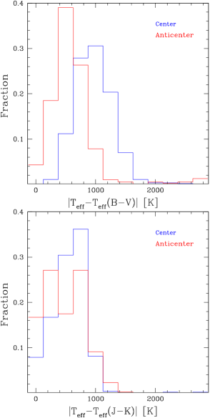
Figure 14: Upper panel: histograms of the difference between photometric $T_{\rm{eff}}(B-V)$ and spectroscopic $T_{\rm{eff}}$ for the sample of Gazzano et al. (2010). Lower panel: histograms of the difference between photometric $T_{\rm{eff}}(J-K)$ and spectroscopic $T_{\rm{eff}}$ for the sample of Gazzano et al. (2010).

4.4 The iron and Li abundances and three Li-rich giants

Figure 15 shows that our values of $\rm{[Fe/H]}$ strongly agree with typical values found in the Galactic disk, which range from $-1.3$ to $+0.4$ (Reddy et al., 2006; Bensby et al., 2007; Meléndez et al., 2008). In fact, as was mentioned before, differences are expected in the distributions of $\rm{[Fe/H]}$ between both CoRoT fields. As shown in Fig. 2, the $\rm{LRc}01$ field is composed of stars with lower $\rm{[Fe/H]}$ values than the $\rm{LRa}01$ field. Stars with $\rm{[Fe/H]}$ $<0.0$ represent $75\%$ and $56\%$ of the sample in the $\rm{LRc}01$ and $\rm{LRa}01$ fields, respectively. Following this point, stars in those CoRoT fields also present important differences in the distribution of $T_{\rm{eff}}$ , $\log\,(g)$ , and evolutionary stages, suggesting a link with $\rm{[Fe/H]}$ . This can be seen when the histograms for each evolutionary stage are analyzed (see Fig. 15). The mean values of $\rm{[Fe/H]}$ for stars in the MS, SGB, and RGB of the $\rm{LRc}01$ field are $+0.05$, $-0.16$, and $-0.26$, respectively. For the $\rm{LRa}01$ field, the corresponding mean values are $+0.04$, $-0.02$, and $-0.41$.

Our $\rm{[Fe/H]}$ distributions show a similar behavior to that presented by Gazzano et al. (2010) in an extensive spectroscopic survey of the CoRoT field. Similarly, our results show that most stars on the MS present solar $\rm{[Fe/H]}$ values, whereas most stars in evolved stages have low metallicities. The relation between $\rm{[Fe/H]}$ , evolutionary stages, and the two different Galactic directions observed by CoRoT found in Gazzano et al. (2010) , which we confirmed, could be explained by the metallicity gradient found in the Galactic disk (Pedicelli et al., 2009; Friel et al., 2010; Luck et al., 2011).

The behavior of the lithium abundances for the stars in our sample is shown in Fig. 16, with the $A(\rm{Li})$ distribution along the HR diagram in the upper panel and histograms for different evolutionary stages in the lower panel. The $A(\rm{Li})$ measurements for the present stellar sample clearly follows the well-established scenario for the lithium behavior at the referred evolutionary phases (Luck, 1977; Boesgaard & Tripicco, 1986; Soderblom et al., 1993; Wallerstein et al., 1994; de Medeiros et al., 1997; Lèbre et al., 1999; De Medeiros et al., 2000; Meléndez et al., 2010).

Indeed, the stellar lithium content is extremely sensitive to the physical conditions inside stars. As well established, the surface Li abundance is further depleted after stars leave the MS and undergo the first dredge-up (Iben, 1967a, b). As a result, RGB stars essentially exhibit low $A(\rm{Li})$ (Brown et al., 1989). Nevertheless, an increasing list of studies report the discovery of giant stars violating this rule (e.g., Wallerstein & Sneden, 1982; Brown et al., 1989; Pilachowski et al., 2000; Martell & Shetrone, 2013), the so-called lithium-rich giant stars, which present atypically large lithium abundances, in contrast to theoretical predictions. Three stars in the present CoRoT sample show this an abnormal lithium behavior: CoRoT ID $100537408$, with an $A(\rm{Li})$ of $1.45\pm 0.46$; CoRoT ID $101358013$, with an $A(\rm{Li})$ of $2.27\pm 0.21$; and CoRoT ID $101555541$, with an $A(\rm{Li})$ of $1.13\pm 0.18$ (see Fig. 16).

Figure 17 shows the distributions of $A(\rm{Li})$ for the whole sample located in the Galactic center and anti–center directions. The upper panel of Fig. 17 provides an indication that a difference may be present, with the highest lithium content in the anti-center direction and an apparent bimodal distribution in the center direction. However, the histograms for the stars segregated by MS, SGB, and RGB evolutionary stages (bottom panel) show no statistically clear difference between Galactic center and anti–center. Indeed, the distributions of $A(\rm{Li})$ for stars separated by evolutionary stages seem to indicate that the behavior of the lithium content observed along the HR diagram follows the same trend irrespective of the location of stars in Galactic center or anti-center directions.

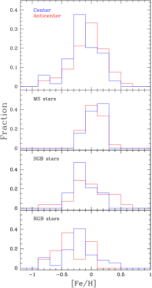
Figure 15: Upper panel: histogram of the iron abundances $\rm{[Fe/H]}$ in the CoRoT fields. Lower panels: histograms of the iron abundances $\rm{[Fe/H]}$ for the different evolutionary stages. A relation between $\rm{[Fe/H]}$ and evolutionary status is clearly present for the stars in our sample. Stars with abnormal lithium behavior are presented using filled circles.

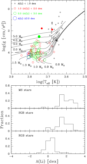
Figure 16: Upper panel: distribution of $A(\rm{Li})$ along the HR diagram for the stars of the present sample. Symbol size is proportional to the value of $A(\rm{Li})$ . The stars showing an abnormal lithium behavior are presented using filled circles. Evolutionary tracks are the same as in Fig. 7. Lower panels: histograms of $A(\rm{Li})$ for different evolutionary stages.

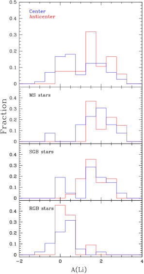
Figure 17: Upper panel: histogram of the lithium abundances $A(\rm{Li})$ in the CoRoT fields with stars segregated in the two Galactic directions, with blue indicating the Center and red the Anti–center. Lower panels: histograms of A(Li) for different evolutionary stages.

5 Conclusions

We present physical parameters ($T_{\rm{eff}}$ , $\log\,(g)$ , $v_{\rm{mic}}$ , and $v\sin\,(i)$ ), dynamical properties ($v_{\rm{rad}}$ ), and chemical abundances ( $\rm{[Fe/H]}$ and $A(\rm{Li})$ ) for a sample of 138 stars stars located in the CoRoT Exoplanetary fields LRc01 and LRa01, based on observations collected with UVES/VLT at ESO and Hydra/Blanco at CTIO. The derived parameters allow us to characterize physically the observed stellar sample, with the stars located in different regions of the HR diagram, from the MS to well-evolved stages, including the SGB and RGB. We also provide estimates of possible errors in the temperatures derived using photometric calibrations, and also of reddening values for the stars in the aforementioned CoRoT fields.

Our results show a relation between $T_{\rm{eff}}$ , evolutionary stage, and $\rm{[Fe/H]}$ in the CoRoT fields, which is related to the color distributions in these fields. These results are in agreement with independent photometric and spectroscopic surveys of the CoRoT fields. These results give support to our spectroscopically-determined parameters. Our chemical analysis shows that the stars in the CoRoT fields present the same patterns found and reported on for the Galactic disk, showing a mixture of different populations associated with the Milky Way.

The stellar sample presents the same rotational behavior described in the literature for different evolutionary stages and colors. Also, we provide a calibration to derive $v\sin\,(i)$ from Hydra observations using the robust CCF technique (see section 3.2 and eq. 3).

Finally, the present data set also represents an important piece of work to be used as standard sample calibration for different programs in the context of the CoRoT mission, since, among the brightest stars that comprise the CoRoT exoplanet field targets, dozens are included in the list of stars analyzed here. It is important to remark this work also can help to increase the scientific return of other spacial missions, such as Gaia or TESS.

Table 1: CoRoT IDs, ephemerides, details of observations, photometry, and estimated luminosity classes (LC) for the UVES stars .

CoRoT ID	RA	DEC	Heliocentric Julian Date	$\rm{T_{exp}}$	$S/N$	$V$	$(B-V)$	$J$	$H$	$K$	LC	Field
	(J2000)	(J2000)	(HJD)	(s)		(mag)	(mag)	(mag)	(mag)	(mag)
100532655	$19:23:03.\!118$	$+01:34:55.\!60$	2006 Apr 23	$1000$	$128$	$12.\!03$	$0.\!93$	$10.\!38$	$10.\!01$	$9.\!93$	IV	LRc01
100537408	$19:23:04.\!841$	$+01:46:24.\!49$	2006 May 16	$1000$	$130$	$12.\!23$	$0.\!85$	$10.\!60$	$10.\!36$	$10.\!22$	III	LRc01
100931549	$19:25:21.\!353$	$+00:11:07.\!94$	2006 May 23	$1000$	$129$	$12.\!48$	$0.\!89$	$10.\!93$	$10.\!58$	$10.\!48$	IV	LRc01
100932329	$19:25:21.\!593$	$+00:11:31.\!02$	2006 May 23	$1000$	$200$	$12.\!12$	$1.\!01$	$10.\!33$	$9.\!88$	$9.\!76$	IV	LRc01
101041358	$19:26:00.\!737$	$+00:36:33.\!01$	2006 Jun 17	$1000$	$131$	$12.\!43$	$0.\!90$	$10.\!71$	$10.\!27$	$10.\!18$	V	LRc01
101043867	$19:26:01.\!891$	$-00:02:49.\!67$	2006 Jun 17	$1000$	$111$	$12.\!42$	$0.\!85$	$10.\!83$	$10.\!49$	$10.\!43$	IV	LRc01
101056542	$19:26:07.\!651$	$+00:11:03.\!37$	2006 Jun 17	$1000$	$122$	$12.\!43$	$0.\!67$	$11.\!14$	$10.\!90$	$10.\!85$	IV	LRc01
101076647	$19:26:17.\!654$	$+00:12:09.\!00$	2006 Apr 19	$1000$	$102$	$12.\!43$	$0.\!90$	$10.\!73$	$10.\!40$	$10.\!32$	IV	LRc01
101102758	$19:26:27.\!502$	$+00:32:20.\!15$	2006 Apr 23	$1000$	$124$	$12.\!43$	$1.\!00$	$10.\!62$	$10.\!24$	$10.\!10$	IV	LRc01
101128747	$19:26:37.\!291$	$+00:02:58.\!96$	2006 Jun 17	$1000$	$141$	$12.\!00$	$0.\!87$	$10.\!46$	$10.\!22$	$10.\!11$	III	LRc01
101204408	$19:27:05.\!707$	$+00:32:05.\!06$	2006 Jun 17	$1000$	$142$	$13.\!58$	$1.\!52$	$10.\!74$	$10.\!00$	$9.\!86$	V	LRc01
101208246	$19:27:07.\!138$	$+00:27:19.\!33$	2006 Jun 17	$1000$	$109$	$12.\!43$	$1.\!02$	$10.\!61$	$10.\!20$	$10.\!08$	IV	LRc01
101231832	$19:27:16.\!032$	$+00:17:35.\!59$	2006 Jun 17	$1000$	$150$	$12.\!13$	$0.\!90$	$10.\!47$	$10.\!08$	$10.\!02$	IV	LRc01
101462309	$19:28:53.\!256$	$-00:04:41.\!20$	2006 Jun 18	$1000$	$130$	$12.\!13$	$0.\!89$	$10.\!55$	$10.\!22$	$10.\!15$	V	LRc01
101476063	$19:28:58.\!836$	$+00:40:16.\!72$	2006 Jun 18	$1000$	$105$	$12.\!20$	$0.\!97$	$10.\!46$	$10.\!07$	$9.\!93$	III	LRc01
101478005	$19:28:59.\!618$	$-00:07:21.\!76$	2006 Jun 18	$1000$	$120$	$12.\!24$	$0.\!99$	$10.\!52$	$10.\!07$	$9.\!99$	IV	LRc01
101565378	$19:29:35.\!662$	$-00:12:26.\!06$	2006 May 30	$1000$	$174$	$12.\!33$	$0.\!80$	$10.\!87$	$10.\!56$	$10.\!47$	IV	LRc01
101613938	$19:29:56.\!532$	$+00:01:31.\!04$	2006 May 30	$1000$	$167$	$12.\!23$	$0.\!86$	$10.\!70$	$10.\!40$	$10.\!35$	V	LRc01
101697676	$19:30:35.\!563$	$+00:03:20.\!05$	2006 May 30	$1000$	$153$	$12.\!37$	$0.\!80$	$10.\!99$	$10.\!67$	$10.\!60$	V	LRc01
102585563	$06:41:02.\!086$	$-00:33:16.\!38$	2006 Sept 07	$1000$	$166$	$16.\!12$	$1.\!08$	$13.\!71$	$13.\!09$	$12.\!99$	V	LRa01
102585613	$06:41:02.\!184$	$+00:19:38.\!39$	2006 Sept 06	$1000$	$188$	$12.\!34$	$0.\!44$	$11.\!31$	$11.\!11$	$11.\!03$	III	LRa01
102589564	$06:41:08.\!995$	$+00:48:20.\!41$	2006 Sept 07	$1000$	$133$	$12.\!46$	$0.\!50$	$11.\!49$	$11.\!29$	$11.\!21$	V	LRa01
102591896	$06:41:12.\!994$	$-00:45:13.\!54$	2006 Sept 03	$1000$	$150$	$12.\!25$	$0.\!54$	$11.\!28$	$11.\!09$	$11.\!00$	V	LRa01
102603174	$06:41:31.\!006$	$-00:57:44.\!14$	2006 Sept 10	$1000$	$138$	$12.\!08$	$0.\!56$	$11.\!14$	$10.\!86$	$10.\!81$	V	LRa01
102604055	$06:41:32.\!222$	$+00:59:10.\!75$	2006 Sept 10	$1000$	$126$	$12.\!35$	$0.\!46$	$11.\!41$	$11.\!21$	$11.\!15$	V	LRa01
102605405	$06:41:34.\!037$	$+00:00:30.\!24$	2006 Sept 13	$1000$	$211$	$12.\!08$	$0.\!60$	$10.\!97$	$10.\!69$	$10.\!63$	V	LRa01
102606185	$06:41:35.\!021$	$+00:54:44.\!68$	2006 Sept 13	$1000$	$105$	$13.\!44$	$0.\!56$	$12.\!39$	$12.\!11$	$12.\!10$	V	LRa01
102611980	$06:41:42.\!962$	$-00:24:33.\!84$	2006 Sept 13	$1000$	$117$	$12.\!41$	$0.\!65$	$11.\!30$	$11.\!00$	$10.\!97$	V	LRa01
102614844	$06:41:46.\!882$	$+00:21:40.\!72$	2006 Sept 22	$1000$	$91$	$12.\!50$	$0.\!83$	$11.\!13$	$10.\!78$	$10.\!72$	IV	LRa01
102616719	$06:41:49.\!716$	$-01:32:02.\!26$	2006 Aug 31	$1000$	$123$	$12.\!31$	$0.\!59$	$11.\!30$	$11.\!08$	$10.\!99$	V	LRa01
102618948	$06:41:52.\!913$	$+00:24:13.\!86$	2006 Sept 22	$1000$	$134$	$12.\!01$	$0.\!66$	$10.\!88$	$10.\!63$	$10.\!55$	III	LRa01
102620828	$06:41:55.\!704$	$-00:59:37.\!90$	2006 Sept 24	$1000$	$120$	$12.\!36$	$0.\!85$	$10.\!90$	$10.\!47$	$10.\!37$	III	LRa01
102654716	$06:42:42.\!254$	$+00:47:29.\!00$	2006 Sept 23	$1000$	$171$	$12.\!15$	$0.\!55$	$11.\!06$	$10.\!83$	$10.\!74$	III	LRa01
102657182	$06:42:45.\!377$	$-00:32:21.\!05$	2006 Sept 24	$1000$	$116$	$12.\!35$	$0.\!78$	$10.\!98$	$10.\!60$	$10.\!55$	III	LRa01
102658181	$06:42:46.\!610$	$+00:53:40.\!09$	2006 Sept 24	$1000$	$103$	$12.\!38$	$0.\!71$	$11.\!12$	$10.\!80$	$10.\!73$	V	LRa01
102659670	$06:42:48.\!432$	$+00:29:03.\!59$	2006 Sept 25	$1000$	$129$	$12.\!01$	$0.\!51$	$11.\!07$	$10.\!85$	$10.\!81$	III	LRa01
102663892	$06:42:53.\!772$	$-01:17:53.\!56$	2006 Sept 27	$1000$	$145$	$12.\!36$	$0.\!60$	$11.\!31$	$11.\!03$	$10.\!98$	V	LRa01
102669038	$06:43:00.\!288$	$+00:49:01.\!52$	2006 Sept 26	$750$	$112$	$12.\!38$	$0.\!46$	$11.\!37$	$11.\!17$	$11.\!09$	III	LRa01
102669801	$06:43:01.\!198$	$+00:14:26.\!81$	2006 Sept 25	$1000$	$111$	$12.\!34$	$0.\!66$	$11.\!10$	$10.\!80$	$10.\!73$	III	LRa01
102676872	$06:43:09.\!950$	$-01:27:26.\!03$	2006 Sept 25	$1000$	$120$	$12.\!19$	$0.\!98$	$10.\!28$	$9.\!81$	$9.\!68$	III	LRa01
102678564	$06:43:12.\!110$	$-00:26:59.\!78$	2006 Sept 25	$1000$	$130$	$12.\!11$	$0.\!51$	$11.\!13$	$10.\!93$	$10.\!86$	V	LRa01
102679796	$06:43:13.\!630$	$+00:45:08.\!89$	2006 Sept 25	$1000$	$127$	$12.\!04$	$0.\!50$	$11.\!06$	$10.\!83$	$10.\!79$	IV	LRa01
102686019	$06:43:21.\!432$	$-00:04:27.\!05$	2006 Sept 25	$1000$	$130$	$12.\!20$	$0.\!50$	$11.\!30$	$11.\!07$	$11.\!02$	V	LRa01
102687759	$06:43:23.\!638$	$+00:12:21.\!89$	2006 Sept 26	$1000$	$140$	$12.\!21$	$0.\!56$	$11.\!14$	$10.\!86$	$10.\!85$	V	LRa01
102692093	$06:43:29.\!011$	$+01:02:31.\!52$	2006 Oct 01	$1000$	$132$	$12.\!47$	$0.\!61$	$11.\!25$	$10.\!94$	$10.\!87$	III	LRa01
102705308	$06:43:44.\!971$	$+00:55:50.\!41$	2006 Sept 27	$1000$	$167$	$12.\!39$	$0.\!96$	$10.\!59$	$10.\!09$	$10.\!00$	III	LRa01
102709247	$06:43:50.\!210$	$-01:11:03.\!01$	2006 Sept 27	$1000$	$142$	$12.\!46$	$0.\!77$	$11.\!25$	$10.\!91$	$10.\!88$	III	LRa01
102718064	$06:44:02.\!532$	$+00:27:04.\!14$	2006 Sept 27	$1000$	$167$	$15.\!91$	$0.\!73$	$14.\!41$	$14.\!26$	$13.\!91$	V	LRa01
102738854	$06:44:31.\!608$	$-00:18:21.\!10$	2006 Sept 27	$1000$	$126$	$12.\!25$	$0.\!63$	$11.\!12$	$10.\!85$	$10.\!80$	IV	LRa01
102740520	$06:44:33.\!814$	$-00:50:35.\!77$	2006 Sept 05	$1000$	$103$	$12.\!40$	$0.\!79$	$11.\!19$	$10.\!88$	$10.\!82$	V	IRa01
102741215	$06:44:34.\!738$	$-01:55:45.\!69$	2006 Sept 05	$1000$	$126$	$12.\!41$	$0.\!63$	$11.\!25$	$10.\!97$	$10.\!91$	V	LRa01
102764866	$06:45:06.\!610$	$-01:05:31.\!81$	2006 Sept 28	$1000$	$150$	$12.\!14$	$0.\!63$	$11.\!01$	$10.\!71$	$10.\!63$	IV	LRa01
102772347	$06:45:16.\!702$	$-00:56:54.\!06$	2006 Sept 28	$1000$	$142$	$12.\!14$	$0.\!66$	$10.\!97$	$10.\!65$	$10.\!59$	IV	LRa01

Table 2: Setup used for Hydra observations.

Field	Number of exposures	$T_{\rm{exp}}$	Heliocentric Julian Date	Filter
		(s)	(HDJ)
$LRa01$	$2$	$2700$	2009 Oct 04	$E5187$
$LRc01$	$2$	$2700$	2009 Oct 04	$E5187$
$LRa01$	$2$	$2200$	2009 Oct 04	$E6757$
$LRc01$	$2$	$2850$	2009 Oct 04	$E6757$

Table 3: The main characteristics for the Hydra stars .

CoRoT ID	RA	DEC	$S/N$	$V$	$(B-V)$	$J$	$H$	$K$	LC	Field
	(J2000)	(J2000)		(mag)	(mag)	(mag)	(mag)	(mag)
101057962	$19:26:08.33$	$-00:25:22.80$	$167$	$12.69$	$1.44$	$9.95$	$9.22$	$9.07$	V	LRc01
101066444	$19:26:12.18$	$+00:01:28.60$	$123$	$13.37$	$1.81$	$10.04$	$9.25$	$9.03$	II	LRc01
101124344	$19:26:35.61$	$-00:27:25.00$	$187$	$13.18$	$1.24$	$10.92$	$10.39$	$10.26$	III	LRc01
101154362	$19:26:46.93$	$-00:12:23.80$	$170$	$13.13$	$1.34$	$10.77$	$10.13$	$9.98$	V	LRc01
101165983	$19:26:51.33$	$-00:11:36.20$	$85$	$13.55$	$1.40$	$10.98$	$10.28$	$10.12$	V	LRc01
101178248	$19:26:55.94$	$+00:06:04.30$	$168$	$12.38$	$1.48$	$9.71$	$9.04$	$8.83$	V	LRc01
101237841	$19:27:18.30$	$-00:18:36.60$	$158$	$12.71$	$1.47$	$9.99$	$9.24$	$9.04$	V	LRc01
101249643	$19:27:22.85$	$-00:11:34.00$	$141$	$13.15$	$0.75$	$11.71$	$11.37$	$11.32$	IV	LRc01
101258619	$19:27:26.19$	$-00:00:00.90$	$132$	$12.76$	$1.28$	$10.46$	$9.84$	$9.73$	V	LRc01
101268962	$19:27:30.19$	$+00:05:46.20$	$91$	$13.45$	$1.28$	$11.05$	$10.43$	$10.32$	V	LRc01
101305750	$19:27:43.47$	$-00:23:44.20$	$120$	$13.25$	$1.25$	$11.02$	$10.46$	$10.36$	IV	LRc01
101319580	$19:27:49.44$	$-00:13:25.20$	$118$	$12.64$	$1.42$	$10.15$	$9.58$	$9.41$	V	LRc01
101346995	$19:28:02.83$	$+00:20:23.39$	$105$	$13.19$	$1.68$	$10.11$	$9.37$	$9.13$	II	LRc01
101347642	$19:28:03.14$	$-00:21:33.90$	$93$	$12.72$	$1.44$	$10.15$	$9.54$	$9.37$	V	LRc01
101347760	$19:28:03.20$	$+00:16:07.32$	$123$	$13.03$	$1.20$	$10.63$	$10.09$	$9.92$	V	LRc01
101358013	$19:28:08.16$	$-00:20:27.30$	$128$	$12.65$	$0.85$	$10.93$	$10.56$	$10.47$	IV	LRc01
101392071	$19:28:24.37$	$+00:04:02.39$	$99$	$12.96$	$1.70$	$9.89$	$9.14$	$8.87$	III	LRc01
101411168	$19:28:32.30$	$+00:08:48.98$	$176$	$12.45$	$1.44$	$9.87$	$9.23$	$9.05$	V	LRc01
101421386	$19:28:36.46$	$+00:13:53.22$	$78$	$13.08$	$1.27$	$10.66$	$10.05$	$9.90$	V	LRc01
101422730	$19:28:37.00$	$+00:35:47.90$	$116$	$13.44$	$1.41$	$10.91$	$10.28$	$10.08$	III	LRc01
101423629	$19:28:37.35$	$+00:08:34.15$	$92$	$13.39$	$1.49$	$10.73$	$10.07$	$9.88$	V	LRc01
101433432	$19:28:41.46$	$+00:02:59.42$	$144$	$13.52$	$1.47$	$10.88$	$10.25$	$10.07$	V	LRc01
101451115	$19:28:48.69$	$+00:05:19.28$	$151$	$13.39$	$1.38$	$10.79$	$10.10$	$9.93$	V	LRc01
101455904	$19:28:50.63$	$+00:01:43.21$	$132$	$12.95$	$0.94$	$11.34$	$10.92$	$10.83$	V	LRc01
101458937	$19:28:51.90$	$+00:10:25.10$	$144$	$13.22$	$1.52$	$10.39$	$9.70$	$9.48$	V	LRc01
101461526	$19:28:52.93$	$+00:03:52.74$	$145$	$13.44$	$1.63$	$10.43$	$9.65$	$9.42$	II	LRc01
101464585	$19:28:54.20$	$+00:27:25.52$	$114$	$13.49$	$1.70$	$10.39$	$9.61$	$9.35$	II	LRc01
101479386	$19:29:00.19$	$+00:27:51.30$	$156$	$13.01$	$1.51$	$10.26$	$9.60$	$9.42$	V	LRc01
101483826	$19:29:02.05$	$+00:25:04.22$	$123$	$12.71$	$1.44$	$10.08$	$9.46$	$9.30$	V	LRc01
101489251	$19:29:04.27$	$+00:35:50.71$	$134$	$13.10$	$1.79$	$9.81$	$8.98$	$8.72$	II	LRc01
101489977	$19:29:04.55$	$+00:25:45.62$	$127$	$13.04$	$1.51$	$10.45$	$9.81$	$9.63$	I	LRc01
101492953	$19:29:05.79$	$+00:09:00.32$	$158$	$12.68$	$1.29$	$10.38$	$9.78$	$9.59$	V	LRc01
101519854	$19:29:16.94$	$+00:03:50.33$	$140$	$13.27$	$1.08$	$11.34$	$10.92$	$10.86$	IV	LRc01
101536086	$19:29:23.83$	$+00:37:03.72$	$120$	$13.14$	$1.38$	$10.64$	$9.97$	$9.87$	V	LRc01
101538522	$19:29:24.87$	$-00:00:17.75$	$157$	$13.02$	$1.63$	$9.94$	$9.16$	$8.94$	III	LRc01
101549180	$19:29:29.41$	$+00:00:11.41$	$169$	$12.13$	$0.82$	$10.59$	$10.28$	$10.18$	V	LRc01
101550759	$19:29:30.06$	$+00:04:39.07$	$117$	$13.13$	$1.45$	$10.54$	$9.88$	$9.70$	V	LRc01
101552742	$19:29:30.81$	$+00:15:15.48$	$137$	$13.43$	$1.32$	$10.87$	$10.28$	$10.11$	V	LRc01
101555541	$19:29:31.89$	$+00:23:40.09$	$123$	$12.63$	$1.38$	$10.08$	$9.41$	$9.27$	V	LRc01
101561050	$19:29:34.00$	$+00:15:32.94$	$105$	$12.47$	$1.47$	$9.78$	$9.11$	$8.92$	V	LRc01
101562508	$19:29:34.56$	$+00:08:29.36$	$130$	$13.14$	$1.39$	$10.61$	$9.97$	$9.79$	V	LRc01
101565091	$19:29:35.55$	$+00:36:32.08$	$224$	$12.60$	$0.98$	$10.75$	$10.41$	$10.30$	I	LRc01
101569925	$19:29:37.39$	$+00:30:53.71$	$111$	$13.16$	$1.45$	$10.54$	$9.92$	$9.74$	V	LRc01
101598546	$19:29:49.09$	$+00:25:32.38$	$125$	$13.53$	$1.51$	$10.83$	$10.20$	$10.06$	V	LRc01
101599646	$19:29:49.59$	$+00:18:20.16$	$95$	$12.93$	$0.86$	$11.26$	$10.95$	$10.85$	V	LRc01
101600807	$19:29:50.14$	$+00:27:10.40$	$98$	$12.99$	$1.55$	$10.18$	$9.51$	$9.35$	V	LRc01
101612300	$19:29:55.73$	$+00:15:20.70$	$131$	$12.67$	$1.08$	$10.59$	$10.16$	$10.06$	IV	LRc01
101622447	$19:30:00.67$	$+00:27:25.34$	$102$	$13.51$	$1.50$	$10.76$	$10.12$	$9.95$	V	LRc01
101626971	$19:30:02.86$	$+00:06:48.31$	$154$	$13.30$	$1.32$	$10.74$	$10.17$	$10.00$	V	LRc01
101627005	$19:30:02.88$	$+00:24:24.41$	$110$	$12.93$	$0.98$	$11.09$	$10.77$	$10.67$	IV	LRc01
101635594	$19:30:07.24$	$+00:25:09.41$	$78$	$13.49$	$1.74$	$10.36$	$9.66$	$9.46$	III	LRc01
101642292	$19:30:10.61$	$+00:03:55.08$	$132$	$12.61$	$1.47$	$10.00$	$9.35$	$9.17$	V	LRc01
101665008	$19:30:21.98$	$+00:18:46.55$	$111$	$13.56$	$1.45$	$10.83$	$10.19$	$9.99$	V	LRc01
102574603	$06:40:43.20$	$+00:51:16.10$	$87$	$12.37$	$0.58$	$11.26$	$11.00$	$10.92$	III	LRa01
102580280	$06:40:52.98$	$+00:39:57.30$	$150$	$13.20$	$0.73$	$11.70$	$11.33$	$11.23$	III	LRa01
102586626	$06:41:03.94$	$+00:59:26.00$	$177$	$12.30$	$1.25$	$9.87$	$9.24$	$9.09$	III	LRa01
102598042	$06:41:23.33$	$+00:53:08.70$	$60$	$13.30$	$0.79$	$11.92$	$11.54$	$11.48$	IV	LRa01
102602960	$06:41:30.72$	$+00:40:55.50$	$97$	$13.10$	$0.63$	$11.86$	$11.59$	$11.48$	V	LRa01
102612876	$06:41:44.23$	$+00:27:46.00$	$124$	$13.08$	$1.29$	$10.44$	$9.77$	$9.61$	III	LRa01
102615343	$06:41:47.66$	$+00:45:43.50$	$62$	$13.02$	$0.54$	$11.97$	$11.71$	$11.69$	V	LRa01
102625766	$06:42:03.03$	$+00:39:04.40$	$77$	$12.69$	$0.57$	$11.61$	$11.33$	$11.27$	III	LRa01
102627939	$06:42:06.25$	$+00:29:57.90$	$150$	$13.15$	$0.77$	$11.77$	$11.46$	$11.37$	III	LRa01
102637778	$06:42:20.33$	$+00:31:50.70$	$96$	$13.24$	$0.67$	$12.00$	$11.68$	$11.60$	III	LRa01
102662415	$06:42:51.90$	$+00:33:40.30$	$120$	$12.98$	$1.08$	$11.03$	$10.52$	$10.38$	III	LRa01
102694697	$06:43:32.20$	$-00:32:21.95$	$133$	$12.36$	$1.25$	$10.10$	$9.49$	$9.35$	III	LRa01
102694848	$06:43:32.40$	$-00:38:31.13$	$96$	$12.61$	$1.38$	$10.15$	$9.52$	$9.32$	III	LRa01
102695542	$06:43:33.28$	$-00:39:35.24$	$170$	$12.62$	$1.09$	$10.46$	$10.01$	$9.85$	III	LRa01
102697221	$06:43:35.29$	$-00:43:32.74$	$200$	$12.12$	$1.23$	$9.93$	$9.30$	$9.16$	III	LRa01
102705009	$06:43:44.57$	$-00:29:03.05$	$138$	$12.19$	$0.67$	$11.05$	$10.74$	$10.69$	V	LRa01
102705076	$06:43:44.66$	$-00:44:53.84$	$60$	$13.28$	$0.75$	$11.89$	$11.48$	$11.39$	III	LRa01
102706020	$06:43:45.85$	$-00:36:23.76$	$94$	$12.67$	$1.12$	$10.52$	$9.95$	$9.81$	III	LRa01
102728377	$06:44:17.43$	$-00:29:26.84$	$103$	$11.83$	$0.58$	$10.77$	$10.48$	$10.41$	V	LRa01
102730409	$06:44:20.10$	$-00:43:49.40$	$76$	$13.14$	$0.63$	$11.98$	$11.69$	$11.63$	III	LRa01
102735621	$06:44:27.19$	$-00:27:49.75$	$84$	$12.86$	$0.64$	$11.69$	$11.42$	$11.35$	III	LRa01
102740367	$06:44:33.64$	$-00:44:07.62$	$120$	$13.24$	$0.70$	$11.98$	$11.66$	$11.59$	V	LRa01
102743491	$06:44:37.76$	$-00:23:37.21$	$90$	$13.10$	$0.82$	$11.64$	$11.29$	$11.20$	III	LRa01
102743929	$06:44:38.32$	$-00:33:34.34$	$122$	$12.60$	$1.14$	$10.53$	$9.96$	$9.80$	III	LRa01
102754990	$06:44:53.16$	$-00:38:04.13$	$114$	$12.26$	$1.18$	$10.03$	$9.45$	$9.33$	III	LRa01
102758371	$06:44:57.73$	$-00:31:03.76$	$134$	$11.62$	$0.56$	$10.61$	$10.34$	$10.31$	III	LRa01
102767494	$06:45:10.17$	$-00:38:53.74$	$95$	$12.98$	$0.74$	$11.64$	$11.27$	$11.24$	V	LRa01
102768747	$06:45:11.82$	$-00:24:49.86$	$97$	$11.74$	$0.63$	$10.61$	$10.30$	$10.22$	V	LRa01
102769088	$06:45:12.28$	$-00:49:14.09$	$105$	$12.00$	$1.22$	$9.80$	$9.25$	$9.10$	III	LRa01
102789493	$06:45:39.68$	$-00:31:59.77$	$62$	$13.47$	$1.12$	$11.34$	$10.84$	$10.66$	III	LRa01
102789962	$06:45:40.31$	$-00:38:06.36$	$99$	$12.40$	$0.51$	$11.47$	$11.27$	$11.22$	III	LRa01
102792032	$06:45:43.18$	$-00:35:51.14$	$108$	$12.25$	$1.23$	$9.90$	$9.28$	$9.13$	III	LRa01

Table 4: The main characteristics and rotation velocities $v\sin\,(i)$ of calibrator stars.

ID	# spectra	$T_{\rm{exp}}$	Date	Hydra Filter	$V$	$(B-V)$	$v\sin\,(i)$	References
		(s)			(mag)	(mag)	${\rm km\,s}^{-1}$
HD 96843	$2$	$600$	2009 Oct 04	$E5187$	$8.36$	$0.66$	$13.0$	$1$
HD 101117	$2$	$600$	2009 Oct 04	$E5187$	$7.87$	$0.59$	$9.0$	$2$
HD 113226	$8$	$7$	2009 Oct 04	$E5187$	$2.83$	$0.93$	$3.0$	$3$
HD 113553	$3$	$600$	2009 Oct 04	$E5187$	$8.33$	$0.68$	$12.0$	$1$
HD 141710	$2$	$600$	2009 Oct 04	$E5187$	$8.93$	$0.14$	$30.0$	$1$
HD 150108	$2$	$600$	2009 Oct 04	$E5187$	$8.23$	$0.84$	$21.0$	$1$
HD 165760	$3$	$30$	2009 Oct 04	$E5187$	$4.67$	$0.95$	$2.6$	$3$
References: (1) Cutispoto et al. 2002; (2) Nordström et al. 2004; (3) Melo et al. 2001

Table 5: Observed broadening $\sigma_{obs}$ and $\sigma_{t}$ for template stars.

ID	# spectra	$<\sigma_{obs}^{P}>$	$\Delta\sigma_{obs}$	$<\sigma_{t}>$
		${\rm km\,s}^{-1}$	${\rm km\,s}^{-1}$	${\rm km\,s}^{-1}$
HD 113226	$8$	$29.9$	$0.6$	$21.2$
HD 165760	$3$	$30.5$	$0.1$	$21.5$

Table 6: Observed broadening $\sigma_{obs}$ and $\sigma_{obs0}$ for calibrator stars.

	Template
	$\rm{HD\leavevmode\nobreak\ 113226}^{a}$		$\rm{HD\leavevmode\nobreak\ 165760}^{b}$
Calibrator	$<\sigma_{obs}>$	$\Delta\sigma_{obs}$	$<\sigma_{obs}>$	$\Delta\sigma_{obs}$	$<\sigma_{obs0}>^{a}$	$<\sigma_{obs0}>^{b}$	$<\sigma_{obs0}>$
	${\rm km\,s}^{-1}$	${\rm km\,s}^{-1}$	${\rm km\,s}^{-1}$	${\rm km\,s}^{-1}$	${\rm km\,s}^{-1}$	${\rm km\,s}^{-1}$	${\rm km\,s}^{-1}$
HD 96843	$33.4$	$0.3$	$33.5$	$0.1$	$25.8$	$25.7$	$25.8$
HD 101117	$32.6$	$0.4$	$32.8$	$0.1$	$24.7$	$24.7$	$24.7$
HD 113226	$...$	$...$	$30.2$	$0.5$	$...$	$21.2$	$21.2$
HD 113553	$33.5$	$0.4$	$33.7$	$0.1$	$25.9$	$25.9$	$25.9$
HD 141710	$46.2$	$0.3$	$46.2$	$0.2$	$41.1$	$40.9$	$41.0$
HD 150108	$37.5$	$0.4$	$37.7$	$0.3$	$31.0$	$30.9$	$31.0$
HD 165760	$30.3$	$0.5$	$...$	$...$	$21.7$	$...$	$21.7$

Table 7: Stellar parameters for the stars in our sample. Refer to sections 3.3 and 4 for details

CoRoT ID	$T_{\rm{eff}}(B-V)$	$T_{\rm{eff}}(J-K)$	$T_{\rm{eff}}$	$\log\,(g)$	$v_{\rm{mic}}$	$\rm{[Fe/H]}$	Fe lines	$A(\rm{Li})$	$v\sin\,(i)$	$v_{\rm{rad}}$	$E(B-V)$	$E(J-K)$	Evol. Status	Inst
	(K)	(K)	(K)	(dex)	(km/s)	(dex)	FeI,FeII	(dex)	${\rm km\,s}^{-1}$	${\rm km\,s}^{-1}$	(mag)	(mag)
	Main Sequence stars
100931549	$5078$	$5571$	$5870^{+105}_{-90}$	$4.08^{+0.13}_{-0.13}$	$1.65^{+0.09}_{-0.09}$	$-0.16\pm 0.04$	$53,7$	$1.96\pm 0.12$	$2^{+1}_{-1}$	$-68.2$	$0.28$	$0.04$	MS	UVES
101057962	$4082$	$3886$	$4640^{+120}_{-110}$	$4.54^{+0.49}_{-0.49}$	$1.68^{+0.42}_{-0.36}$	$0.25\pm 0.15$	$15,4$	$-0.30\pm 0.16$	$3^{+2}_{-2}$	$41.3$	$0.30$	$0.21$	MS	HYDRA
101128747	$5125$	$6161$	$6395^{+65}_{-115}$	$4.11^{+0.25}_{-0.26}$	$1.74^{+0.13}_{-0.11}$	$0.24\pm 0.06$	$54,5$	$3.21\pm 0.12$	$10^{+1}_{-1}$	$-30.8$	$0.39$	$0.03$	MS	UVES
101204408	$3946$	$3886$	$6335^{+54}_{-54}$	$4.05^{+0.28}_{-0.28}$	$1.88^{+0.20}_{-0.29}$	$-0.11\pm 0.04$	$50,11$	$1.75\pm 0.07$	$5^{+1}_{-1}$	$9.2$	$1.02$	$0.55$	MS	UVES
101208246	$4809$	$5167$	$5530^{+30}_{-30}$	$4.44^{+0.16}_{-0.15}$	$1.08^{+0.12}_{-0.12}$	$0.28\pm 0.04$	$61,6$	$1.11\pm 0.03$	$1^{+1}_{-1}$	$-70.4$	$0.30$	$0.06$	MS	UVES
101231832	$5050$	$5571$	$5600^{+50}_{-20}$	$4.28^{+0.15}_{-0.10}$	$1.42^{+0.06}_{-0.04}$	$-0.02\pm 0.02$	$61,7$	$2.01\pm 0.06$	$1^{+1}_{-1}$	$-14.4$	$0.20$	$0.00$	MS	UVES
101319580	$4115$	$4323$	$4650^{+140}_{-190}$	$3.95^{+0.48}_{-0.42}$	$3.97^{+0.93}_{-0.59}$	$0.06\pm 0.15$	$17,3$	$1.03\pm 0.35$	$10^{+2}_{-2}$	$41$	$0.29$	$0.08$	MS	HYDRA
101455904	$4973$	$5263$	$5230^{+370}_{-280}$	$4.68^{+0.40}_{-0.30}$	$0.55^{+0.90}_{-0.55}$	$0.09\pm 0.18$	$18,4$	$2.01\pm 0.53$	$2^{+2}_{-2}$	$-4.9$	$0.10$	$0.00$	MS	HYDRA
101462309	$5065$	$5852$	$5880^{+35}_{-57}$	$4.14^{+0.22}_{-0.20}$	$1.56^{+0.09}_{-0.10}$	$0.14\pm 0.03$	$57,9$	$2.43\pm 0.05$	$3^{+1}_{-1}$	$42.2$	$0.28$	$0.00$	MS	UVES
101476063	$4909$	$5167$	$5780^{+60}_{-55}$	$4.40^{+0.14}_{-0.13}$	$1.44^{+0.07}_{-0.07}$	$0.16\pm 0.03$	$60,5$	$1.84\pm 0.07$	$2^{+1}_{-1}$	$-26$	$0.32$	$0.11$	MS	UVES
101519854	$4689$	$5413$	$5390^{+120}_{-90}$	$4.79^{+0.16}_{-0.17}$	$2.90^{+0.40}_{-0.40}$	$-0.05\pm 0.05$	$13,3$	$1.37\pm 0.18$	$3^{+2}_{-2}$	$61.5$	$0.31$	$0.00$	MS	HYDRA
101612300	$4687$	$5167$	$6050^{+160}_{-200}$	$4.90^{+0.47}_{-0.47}$	$0.47^{+0.80}_{-0.40}$	$0.10\pm 0.06$	$10,4$	$1.75\pm 0.27$	$2^{+2}_{-2}$	$56.6$	$0.51$	$0.16$	MS	HYDRA
101613938	$5146$	$6161$	$6155^{+95}_{-40}$	$4.00^{+0.17}_{-0.17}$	$1.65^{+0.12}_{-0.11}$	$-0.10\pm 0.04$	$51,5$	$2.27\pm 0.08$	$5^{+2}_{-2}$	$-23.7$	$0.32$	$0.00$	MS	UVES
102580280	$5485$	$5465$	$5220^{+50}_{-190}$	$4.52^{+0.16}_{-0.21}$	$1.38^{+1.14}_{-0.48}$	$0.20\pm 0.08$	$16,5$	$\ldots$	$16^{+3}_{-3}$	$57.8$	$\ldots$	$\ldots$	MS	HYDRA
102585563	$4700$	$4393$	$5637^{+38}_{-37}$	$4.53^{+0.37}_{-0.36}$	$1.63^{+0.10}_{-0.10}$	$-0.01\pm 0.04$	$54,7$	$1.62\pm 0.05$	$6^{+1}_{-1}$	$0.3$	$0.39$	$0.27$	MS	UVES
102585613	$6528$	$6646$	$6194^{+276}_{-58}$	$4.25^{+0.24}_{-0.24}$	$1.99^{+0.23}_{-0.30}$	$-0.04\pm 0.05$	$51,5$	$2.59\pm 0.22$	$9^{+1}_{-1}$	$-22.5$	$\ldots$	$\ldots$	MS	UVES
102589564	$6281$	$6646$	$6220^{+80}_{-65}$	$3.90^{+0.28}_{-0.17}$	$1.65^{+0.48}_{-0.63}$	$-0.05\pm 0.05$	$50,9$	$2.35\pm 0.09$	$10^{+1}_{-1}$	$-51.5$	$\ldots$	$\ldots$	MS	UVES
102591896	$6134$	$6646$	$6330^{+80}_{-85}$	$3.99^{+0.33}_{-0.27}$	$2.14^{+0.24}_{-0.34}$	$-0.02\pm 0.07$	$53,10$	$1.55\pm 0.07$	$7^{+1}_{-1}$	$-28.4$	$0.04$	$\ldots$	MS	UVES
102603174	$6044$	$6293$	$6200^{+46}_{-61}$	$3.99^{+0.18}_{-0.29}$	$2.18^{+0.22}_{-0.24}$	$-0.16\pm 0.05$	$50,10$	$1.49\pm 0.03$	$8^{+1}_{-1}$	$-81.7$	$0.03$	$\ldots$	MS	UVES
102604055	$6453$	$6797$	$6397^{+229}_{-80}$	$4.14^{+0.21}_{-0.21}$	$1.60^{+0.29}_{-0.24}$	$-0.25\pm 0.06$	$54,7$	$1.90\pm 0.16$	$9^{+1}_{-1}$	$-12.1$	$\ldots$	$\ldots$	MS	UVES
102605405	$5877$	$6226$	$6100^{+70}_{-134}$	$3.99^{+0.27}_{-0.23}$	$1.53^{+0.09}_{-0.09}$	$0.16\pm 0.04$	$50,9$	$1.50\pm 0.23$	$7^{+1}_{-1}$	$-52.8$	$0.04$	$\ldots$	MS	UVES
102611980	$5725$	$6293$	$5890^{+35}_{-30}$	$4.44^{+0.18}_{-0.24}$	$1.38^{+0.07}_{-0.07}$	$0.01\pm 0.03$	$53,10$	$2.37\pm 0.04$	$3^{+1}_{-1}$	$-21.1$	$0.04$	$\ldots$	MS	UVES
102616719	$5935$	$6430$	$6210^{+57}_{-50}$	$4.30^{+0.24}_{-0.20}$	$1.66^{+0.20}_{-0.12}$	$0.11\pm 0.05$	$58,9$	$2.71\pm 0.06$	$6^{+1}_{-1}$	$-46.3$	$0.06$	$\ldots$	MS	UVES
102618948	$5672$	$6293$	$6110^{+45}_{-40}$	$4.24^{+0.33}_{-0.38}$	$1.55^{+0.08}_{-0.08}$	$0.38\pm 0.05$	$57,10$	$1.30\pm 0.05$	$6^{+1}_{-1}$	$-5.2$	$0.11$	$\ldots$	MS	UVES
102620828	$5160$	$5167$	$5590^{+32}_{-35}$	$4.31^{+0.25}_{-0.20}$	$0.86^{+0.08}_{-0.07}$	$-0.18\pm 0.04$	$60,7$	$\ldots$	$1^{+1}_{-1}$	$2.4$	$0.15$	$0.08$	MS	UVES
102659670	$6223$	$6797$	$6265^{+135}_{-165}$	$3.89^{+0.38}_{-0.39}$	$0.84^{+0.26}_{-0.27}$	$-0.09\pm 0.10$	$54,4$	$1.63\pm 0.17$	$15^{+1}_{-1}$	$-76.1$	$0.00$	$\ldots$	MS	UVES
102663892	$5898$	$6293$	$6130^{+61}_{-69}$	$4.35^{+0.20}_{-0.21}$	$1.36^{+0.10}_{-0.10}$	$0.15\pm 0.04$	$61,11$	$2.71\pm 0.08$	$3^{+1}_{-1}$	$-20.7$	$0.05$	$\ldots$	MS	UVES
102669801	$5682$	$6034$	$5960^{+65}_{-50}$	$4.22^{+0.19}_{-0.23}$	$0.96^{+0.12}_{-0.20}$	$-0.03\pm 0.06$	$55,9$	$2.80\pm 0.09$	$3^{+1}_{-1}$	$-37.8$	$0.07$	$0.00$	MS	UVES
102686019	$6265$	$6646$	$6465^{+99}_{-176}$	$4.12^{+0.34}_{-0.34}$	$1.15^{+0.28}_{-0.17}$	$0.06\pm 0.06$	$54,9$	$1.75\pm 0.15$	$12^{+1}_{-1}$	$-15.4$	$0.03$	$\ldots$	MS	UVES
102687759	$6033$	$6572$	$6390^{+70}_{-90}$	$4.42^{+0.25}_{-0.25}$	$0.80^{+0.56}_{-0.24}$	$-0.04\pm 0.06$	$52,8$	$2.99\pm 0.09$	$5^{+1}_{-1}$	$-20.1$	$0.08$	$\ldots$	MS	UVES
102692093	$5870$	$5972$	$5870^{+50}_{-40}$	$4.41^{+0.14}_{-0.14}$	$1.89^{+0.20}_{-0.26}$	$-0.12\pm 0.05$	$54,4$	$2.77\pm 0.06$	$8^{+1}_{-1}$	$-55.2$	$0.08$	$\ldots$	MS	UVES
102705076	$5414$	$5312$	$5620^{+360}_{-360}$	$4.69^{+0.56}_{-0.48}$	$0.91^{+0.61}_{-0.61}$	$0.04\pm 0.17$	$15,3$	$1.44\pm 0.63$	$11^{+2}_{-2}$	$41.7$	$0.06$	$0.05$	MS	HYDRA
102718064	$5459$	$5312$	$6386^{+106}_{-90}$	$4.44^{+0.32}_{-0.32}$	$0.97^{+0.63}_{-0.20}$	$0.18\pm 0.07$	$55,6$	$3.03\pm 0.11$	$10^{+1}_{-1}$	$-63.8$	$0.24$	$0.18$	MS	UVES
102730409	$5782$	$6161$	$5720^{+270}_{-270}$	$4.63^{+0.47}_{-0.47}$	$1.26^{+0.46}_{-0.46}$	$0.14\pm 0.13$	$17,4$	$2.29\pm 0.37$	$3^{+2}_{-2}$	$59.7$	$\ldots$	$\ldots$	MS	HYDRA
102735621	$5748$	$6226$	$5960^{+330}_{-290}$	$4.57^{+0.49}_{-0.44}$	$2.28^{+0.68}_{-0.68}$	$0.02\pm 0.16$	$14,4$	$2.01\pm 0.38$	$1^{+2}_{-1}$	$12.1$	$0.05$	$\ldots$	MS	HYDRA
102740367	$5571$	$5912$	$5700^{+170}_{-160}$	$4.36^{+0.28}_{-0.23}$	$0.83^{+0.40}_{-0.59}$	$0.03\pm 0.11$	$15,4$	$2.10\pm 0.23$	$12^{+2}_{-2}$	$16.9$	$0.03$	$\ldots$	MS	HYDRA
102741215	$5785$	$6226$	$6985^{+279}_{-185}$	$4.27^{+0.55}_{-0.55}$	$0.59^{+0.37}_{-0.37}$	$0.29\pm 0.13$	$54,11$	$1.70\pm 0.14$	$17^{+1}_{-1}$	$22.8$	$0.28$	$0.10$	MS	UVES
102768747	$5772$	$5912$	$5570^{+230}_{-220}$	$4.64^{+0.30}_{-0.30}$	$1.79^{+0.60}_{-0.50}$	$-0.25\pm 0.12$	$14,4$	$1.61\pm 0.31$	$9^{+2}_{-2}$	$42.3$	$\ldots$	$\ldots$	MS	HYDRA
102789493	$4618$	$4538$	$5600^{+150}_{-150}$	$4.86^{+0.26}_{-0.22}$	$2.65^{+0.80}_{-0.80}$	$0.25\pm 0.08$	$9,4$	$\ldots$	$9^{+2}_{-2}$	$35.1$	$0.42$	$0.23$	MS	HYDRA
102789962	$6236$	$6875$	$6380^{+700}_{-700}$	$4.76^{+0.54}_{-0.54}$	$1.67^{+0.90}_{-0.90}$	$0.11\pm 0.14$	$13,4$	$\ldots$	$10^{+2}_{-2}$	$27.6$	$0.03$	$\ldots$	MS	HYDRA
	Sub-giant Branch stars
100532655	$4976$	$5231$	$5550^{+50}_{-20}$	$3.95^{+0.12}_{-0.12}$	$1.20^{+0.05}_{-0.07}$	$0.28\pm 0.03$	$59,8$	$1.41\pm 0.08$	$1^{+1}_{-1}$	$-36.8$	$0.22$	$0.06$	SGB	UVES
100537408	$5153$	$5552$	$5420^{+110}_{-390}$	$1.60^{+0.36}_{-0.38}$	$0.83^{+0.46}_{-0.70}$	$-0.92\pm 0.11$	$45,5$	$1.45\pm 0.46$	$12^{+1}_{-1}$	$23.6$	$0.08$	$\ldots$	SGB	UVES
100932329	$4823$	$4776$	$5580^{+65}_{-70}$	$3.66^{+0.18}_{-0.12}$	$1.85^{+0.23}_{-0.24}$	$-0.30\pm 0.04$	$56,7$	$2.10\pm 0.09$	$2^{+1}_{-1}$	$-83.6$	$0.31$	$0.19$	SGB	UVES
101041358	$5054$	$4916$	$5750^{+85}_{-60}$	$4.10^{+0.24}_{-0.25}$	$1.69^{+0.18}_{-0.44}$	$-0.33\pm 0.04$	$59,4$	$2.04\pm 0.10$	$3^{+1}_{-1}$	$5.6$	$0.24$	$0.18$	SGB	UVES
101043867	$5162$	$5455$	$6190^{+85}_{-63}$	$3.74^{+0.28}_{-0.24}$	$2.07^{+0.12}_{-0.13}$	$0.19\pm 0.06$	$59,10$	$1.55\pm 0.04$	$5^{+1}_{-1}$	$-18.2$	$0.32$	$0.13$	SGB	UVES
101056542	$5659$	$6041$	$6190^{+85}_{-65}$	$3.82^{+0.21}_{-0.21}$	$2.05^{+0.17}_{-0.13}$	$0.20\pm 0.06$	$59,9$	$1.37\pm 0.11$	$3^{+2}_{-2}$	$-18.2$	$0.14$	$0.02$	SGB	UVES
101076647	$5050$	$5409$	$5905^{+130}_{-105}$	$3.13^{+0.18}_{-0.18}$	$1.73^{+0.41}_{-0.09}$	$-0.03\pm 0.04$	$56,4$	$2.92\pm 0.15$	$8^{+1}_{-1}$	$-58$	$0.30$	$0.09$	SGB	UVES
101102758	$4840$	$4953$	$5760^{+25}_{-25}$	$4.00^{+0.12}_{-0.16}$	$1.73^{+0.09}_{-0.11}$	$0.04\pm 0.03$	$60,7$	$1.94\pm 0.04$	$2^{+1}_{-1}$	$-99.7$	$0.35$	$0.17$	SGB	UVES
101124344	$4411$	$4494$	$4800^{+110}_{-110}$	$2.05^{+0.36}_{-0.37}$	$1.52^{+0.31}_{-0.31}$	$-0.19\pm 0.14$	$18,4$	$0.25\pm 0.10$	$4^{+2}_{-2}$	$11.3$	$0.20$	$0.08$	SGB	HYDRA
101249643	$5420$	$5503$	$5760^{+150}_{-240}$	$4.07^{+0.35}_{-0.32}$	$2.46^{+0.81}_{-0.81}$	$-0.12\pm 0.13$	$13,4$	$\ldots$	$22^{+4}_{-4}$	$21.9$	$0.10$	$0.04$	SGB	HYDRA
101358013	$5153$	$5189$	$5600^{+150}_{-140}$	$2.30^{+0.38}_{-0.35}$	$2.05^{+0.70}_{-0.70}$	$-0.50\pm 0.14$	$12,4$	$2.27\pm 0.21$	$25^{+4}_{-4}$	$10.6$	$0.15$	$0.08$	SGB	HYDRA
101411168	$4084$	$4086$	$4980^{+190}_{-200}$	$1.85^{+0.63}_{-0.60}$	$2.02^{+1.00}_{-0.33}$	$-0.11\pm 0.21$	$17,4$	$0.23\pm 0.32$	$9^{+3}_{-2}$	$-48.2$	$0.48$	$0.29$	SGB	HYDRA
101478005	$4855$	$4916$	$5135^{+20}_{-35}$	$4.17^{+0.13}_{-0.13}$	$0.91^{+0.17}_{-0.07}$	$0.09\pm 0.04$	$59,5$	$0.06\pm 0.05$	$2^{+1}_{-1}$	$-37.4$	$0.11$	$0.05$	SGB	UVES
101549180	$5232$	$5409$	$5180^{+200}_{-200}$	$4.12^{+0.42}_{-0.39}$	$0.56^{+1.00}_{-0.56}$	$-0.34\pm 0.14$	$13,3$	$2.08\pm 0.35$	$30^{+3}_{-3}$	$4.8$	$\ldots$	$\ldots$	SGB	HYDRA
101562508	$4165$	$4086$	$4760^{+100}_{-120}$	$1.37^{+0.42}_{-0.40}$	$1.56^{+0.22}_{-0.18}$	$-0.24\pm 0.09$	$14,4$	$0.70\pm 0.30$	$2^{+2}_{-2}$	$-18.5$	$0.32$	$0.23$	SGB	HYDRA
101565091	$4881$	$5231$	$5690^{+160}_{-140}$	$4.05^{+0.37}_{-0.32}$	$1.91^{+0.99}_{-0.99}$	$-0.15\pm 0.13$	$15,4$	$2.41\pm 0.21$	$1^{+2}_{-1}$	$-36$	$0.31$	$0.09$	SGB	HYDRA
101565378	$5284$	$5455$	$5770^{+200}_{-110}$	$2.89^{+0.41}_{-0.33}$	$1.95^{+0.47}_{-0.33}$	$-0.34\pm 0.14$	$50,9$	$1.41\pm 0.18$	$12^{+1}_{-1}$	$-96.2$	$0.16$	$0.05$	SGB	UVES
101599646	$5128$	$5409$	$5730^{+250}_{-170}$	$3.03^{+0.50}_{-0.53}$	$1.96^{+0.58}_{-0.58}$	$-0.19\pm 0.09$	$12,4$	$\ldots$	$18^{+3}_{-3}$	$-20.4$	$0.20$	$0.06$	SGB	HYDRA
101600807	$3886$	$4063$	$4550^{+160}_{-180}$	$1.44^{+0.66}_{-0.59}$	$1.67^{+0.26}_{-0.21}$	$-0.25\pm 0.14$	$14,4$	$-0.15\pm 0.42$	$6^{+2}_{-2}$	$-43.2$	$0.36$	$0.17$	SGB	HYDRA
101627005	$4883$	$5363$	$5830^{+250}_{-220}$	$3.69^{+0.38}_{-0.38}$	$1.92^{+0.70}_{-0.66}$	$-0.04\pm 0.12$	$13,3$	$1.67\pm 0.33$	$12^{+2}_{-2}$	$-9.9$	$0.35$	$0.08$	SGB	HYDRA
101697676	$5287$	$5503$	$6050^{+240}_{-100}$	$3.87^{+0.26}_{-0.27}$	$1.99^{+0.39}_{-0.28}$	$-0.11\pm 0.07$	$54,7$	$2.49\pm 0.23$	$13^{+1}_{-1}$	$-43.3$	$0.23$	$0.09$	SGB	UVES
102574603	$5980$	$5757$	$5650^{+80}_{-40}$	$3.00^{+0.03}_{-0.03}$	$1.73^{+0.32}_{-0.23}$	$-0.28\pm 0.02$	$14,4$	$2.08\pm 0.09$	$3^{+2}_{-2}$	$-12.8$	$\ldots$	$\ldots$	SGB	HYDRA
102598042	$5302$	$5274$	$5800^{+330}_{-380}$	$3.84^{+0.37}_{-0.41}$	$0.77^{+0.53}_{-0.77}$	$0.45\pm 0.15$	$15,4$	$1.29\pm 0.54$	$1^{+2}_{-1}$	$-24.1$	$0.15$	$0.10$	SGB	HYDRA
102602960	$5772$	$5552$	$5480^{+50}_{-80}$	$4.22^{+0.13}_{-0.06}$	$2.90^{+0.55}_{-0.37}$	$-0.12\pm 0.04$	$18,4$	$2.18\pm 0.11$	$4^{+2}_{-2}$	$58.2$	$\ldots$	$\ldots$	SGB	HYDRA
102606185	$6048$	$6041$	$6185^{+103}_{-116}$	$3.80^{+0.14}_{-0.14}$	$2.02^{+0.11}_{-0.26}$	$0.23\pm 0.05$	$61,10$	$1.70\pm 0.14$	$10^{+1}_{-1}$	$-42.7$	$0.03$	$0.02$	SGB	UVES
102612876	$4333$	$4063$	$4790^{+50}_{-50}$	$1.77^{+0.07}_{-0.10}$	$1.65^{+0.14}_{-0.10}$	$-0.55\pm 0.03$	$13,3$	$0.50\pm 0.15$	$3^{+2}_{-2}$	$42.2$	$0.24$	$0.25$	SGB	HYDRA
102614844	$5198$	$5409$	$5445^{+25}_{-50}$	$4.14^{+0.25}_{-0.19}$	$1.00^{+0.06}_{-0.07}$	$0.37\pm 0.04$	$58,4$	$0.93\pm 0.06$	$1^{+1}_{-1}$	$-3.7$	$0.07$	$0.00$	SGB	UVES
102615343	$6103$	$6101$	$6110^{+250}_{-230}$	$3.65^{+0.11}_{-0.11}$	$0.56^{+1.89}_{-0.56}$	$0.14\pm 0.12$	$13,5$	$2.43\pm 0.30$	$10^{+2}_{-2}$	$58.5$	$0.00$	$0.00$	SGB	HYDRA
102627939	$5362$	$5455$	$5550^{+240}_{-260}$	$3.90^{+0.47}_{-0.22}$	$2.02^{+0.24}_{-0.24}$	$0.07\pm 0.06$	$17,4$	$\ldots$	$7^{+2}_{-2}$	$66$	$0.06$	$0.01$	SGB	HYDRA
102637778	$5640$	$5455$	$5550^{+100}_{-100}$	$3.42^{+0.19}_{-0.20}$	$2.13^{+0.52}_{-1.78}$	$-0.12\pm 0.07$	$18,3$	$1.35\pm 0.15$	$3^{+2}_{-2}$	$5.3$	$\ldots$	$0.01$	SGB	HYDRA
102654716	$6079$	$5867$	$5750^{+55}_{-50}$	$3.25^{+0.42}_{-0.41}$	$0.59^{+0.30}_{-0.26}$	$-0.10\pm 0.06$	$51,5$	$2.23\pm 0.08$	$6^{+1}_{-1}$	$-14$	$\ldots$	$\ldots$	SGB	UVES
102657182	$5338$	$5318$	$5525^{+25}_{-45}$	$4.18^{+0.16}_{-0.16}$	$1.37^{+0.19}_{-0.13}$	$-0.03\pm 0.04$	$61,8$	$1.05\pm 0.02$	$2^{+1}_{-1}$	$-67.9$	$0.06$	$0.03$	SGB	UVES
102658181	$5520$	$5503$	$5655^{+28}_{-23}$	$3.81^{+0.14}_{-0.14}$	$1.28^{+0.04}_{-0.05}$	$0.12\pm 0.04$	$56,4$	$2.01\pm 0.03$	$1^{+1}_{-1}$	$-72.2$	$0.03$	$0.02$	SGB	UVES
102669038	$6436$	$6101$	$6105^{+105}_{-125}$	$3.46^{+0.28}_{-0.28}$	$0.81^{+0.32}_{-0.19}$	$-0.14\pm 0.09$	$54,5$	$1.20\pm 0.13$	$10^{+1}_{-1}$	$-49.6$	$\ldots$	$0.00$	SGB	UVES
102676872	$4881$	$4677$	$5539^{+103}_{-107}$	$3.18^{+0.27}_{-0.15}$	$1.75^{+0.14}_{-0.22}$	$-0.07\pm 0.05$	$60,7$	$1.40\pm 0.14$	$11^{+1}_{-1}$	$-28.1$	$0.26$	$0.21$	SGB	UVES
102678564	$6228$	$6164$	$5900^{+459}_{-212}$	$3.46^{+0.56}_{-0.73}$	$3.57^{+1.60}_{-1.63}$	$-0.71\pm 0.17$	$46,8$	$1.55\pm 0.32$	$17^{+1}_{-1}$	$-4.6$	$\ldots$	$\ldots$	SGB	UVES
102679796	$6286$	$6164$	$6170^{+65}_{-55}$	$3.40^{+0.27}_{-0.22}$	$1.77^{+0.32}_{-0.27}$	$-0.45\pm 0.05$	$41,4$	$1.70\pm 0.06$	$5^{+1}_{-1}$	$-61.5$	$\ldots$	$0.00$	SGB	UVES
102695542	$4673$	$4645$	$5520^{+210}_{-190}$	$1.99^{+0.46}_{-0.47}$	$2.06^{+0.37}_{-0.27}$	$-0.11\pm 0.15$	$14,3$	$\ldots$	$12^{+3}_{-3}$	$46.4$	$0.37$	$0.21$	SGB	HYDRA
102705009	$5653$	$5652$	$5510^{+370}_{-340}$	$3.91^{+0.51}_{-0.50}$	$1.03^{+0.53}_{-0.51}$	$0.13\pm 0.15$	$15,4$	$1.48\pm 0.53$	$4^{+2}_{-2}$	$0.7$	$\ldots$	$\ldots$	SGB	HYDRA
102709247	$5362$	$5601$	$5570^{+38}_{-38}$	$4.00^{+0.14}_{-0.12}$	$0.91^{+0.16}_{-0.05}$	$0.30\pm 0.03$	$53,10$	$1.67\pm 0.04$	$1^{+1}_{-1}$	$-22.9$	$0.06$	$0.00$	SGB	UVES
102728377	$5953$	$5652$	$5820^{+180}_{-170}$	$3.11^{+0.26}_{-0.25}$	$1.16^{+0.22}_{-0.21}$	$-0.10\pm 0.10$	$15,4$	$2.28\pm 0.21$	$8^{+2}_{-2}$	$35$	$\ldots$	$0.02$	SGB	HYDRA
102738854	$5799$	$5867$	$5840^{+80}_{-25}$	$4.05^{+0.24}_{-0.24}$	$1.37^{+0.08}_{-0.11}$	$0.03\pm 0.04$	$57,5$	$1.65\pm 0.05$	$4^{+1}_{-1}$	$-91.9$	$0.00$	$0.00$	SGB	UVES
102740520	$5320$	$5601$	$5640^{+35}_{-32}$	$3.81^{+0.12}_{-0.12}$	$1.28^{+0.14}_{-0.06}$	$0.35\pm 0.04$	$52,7$	$2.49\pm 0.04$	$4^{+1}_{-1}$	$3.9$	$0.10$	$0.00$	SGB	UVES
102743491	$5234$	$5274$	$5990^{+170}_{-120}$	$3.36^{+0.40}_{-0.43}$	$1.63^{+0.58}_{-0.41}$	$0.51\pm 0.06$	$11,4$	$1.20\pm 0.25$	$4^{+2}_{-2}$	$40.6$	$0.23$	$0.13$	SGB	HYDRA
102743929	$4596$	$4302$	$5330^{+250}_{-250}$	$4.03^{+0.20}_{-0.20}$	$2.65^{+0.36}_{-0.36}$	$-0.11\pm 0.09$	$10,4$	$1.25\pm 0.42$	$5^{+2}_{-2}$	$25.6$	$0.34$	$0.29$	SGB	HYDRA
102758371	$6056$	$5981$	$5710^{+130}_{-130}$	$4.01^{+0.18}_{-0.18}$	$1.83^{+0.21}_{-0.20}$	$-0.17\pm 0.07$	$14,3$	$2.39\pm 0.17$	$9^{+2}_{-2}$	$39.9$	$\ldots$	$\ldots$	SGB	HYDRA
102764866	$5789$	$5552$	$5775^{+70}_{-91}$	$3.35^{+0.34}_{-0.32}$	$1.01^{+0.28}_{-0.56}$	$-0.41\pm 0.05$	$53,7$	$\ldots$	$17^{+1}_{-1}$	$-20.1$	$0.00$	$0.04$	SGB	UVES
102772347	$5701$	$5552$	$5970^{+90}_{-90}$	$3.41^{+0.21}_{-0.33}$	$1.58^{+0.23}_{-0.09}$	$0.02\pm 0.06$	$55,10$	$2.40\pm 0.11$	$10^{+1}_{-1}$	$-23.8$	$0.07$	$0.07$	SGB	UVES
102625766	$5987$	$5757$	$5690^{+120}_{-150}$	$3.00^{+0.14}_{-0.15}$	$1.60^{+0.75}_{-0.63}$	$-0.23\pm 0.06$	$14,4$	$1.36\pm 0.16$	$10^{+2}_{-2}$	$4.7$	$\ldots$	$\ldots$	SGB	HYDRA
	Red giant Branch stars
101066444	$2877$	$3714$	$4640^{+120}_{-130}$	$2.72^{+0.72}_{-0.67}$	$2.94^{+0.60}_{-0.29}$	$0.11\pm 0.25$	$11,4$	$0.58\pm 0.16$	$6^{+2}_{-2}$	$12$	$0.68$	$0.38$	RGB	HYDRA
101154362	$4246$	$4155$	$4620^{+170}_{-130}$	$0.16^{+0.70}_{-0.70}$	$1.28^{+0.18}_{-0.18}$	$-0.39\pm 0.22$	$14,4$	$\ldots$	$3^{+2}_{-2}$	$-29.8$	$0.20$	$0.16$	RGB	HYDRA
101165983	$4148$	$3999$	$4200^{+100}_{-100}$	$1.69^{+0.28}_{-0.34}$	$1.34^{+0.09}_{-0.08}$	$-0.16\pm 0.09$	$13,4$	$\ldots$	$4^{+2}_{-2}$	$-44$	$0.00$	$0.07$	RGB	HYDRA
101178248	$4013$	$3957$	$4460^{+120}_{-220}$	$2.11^{+0.41}_{-0.42}$	$2.37^{+0.31}_{-0.24}$	$-0.23\pm 0.14$	$12,4$	$0.85\pm 0.28$	$4^{+2}_{-2}$	$13$	$0.24$	$0.19$	RGB	HYDRA
101237841	$4039$	$3821$	$4210^{+80}_{-70}$	$2.48^{+0.28}_{-0.23}$	$1.88^{+0.07}_{-0.07}$	$-0.34\pm 0.08$	$16,4$	$\ldots$	$1^{+2}_{-1}$	$64.2$	$0.07$	$0.16$	RGB	HYDRA
101258619	$4358$	$4302$	$4950^{+170}_{-80}$	$3.10^{+0.22}_{-0.20}$	$2.25^{+0.18}_{-0.14}$	$-0.04\pm 0.08$	$18,4$	$0.49\pm 0.14$	$7^{+2}_{-2}$	$-17.3$	$0.31$	$0.20$	RGB	HYDRA
101268962	$4358$	$4302$	$4870^{+180}_{-240}$	$2.97^{+0.37}_{-0.42}$	$2.20^{+0.41}_{-0.27}$	$-0.29\pm 0.15$	$16,4$	$0.20\pm 0.53$	$1^{+2}_{-1}$	$11.4$	$0.27$	$0.17$	RGB	HYDRA
101305750	$4406$	$4494$	$4780^{+70}_{-130}$	$2.65^{+0.60}_{-0.63}$	$0.98^{+0.10}_{-0.10}$	$0.31\pm 0.19$	$14,4$	$0.30\pm 0.41$	$6^{+2}_{-2}$	$0.8$	$0.19$	$0.08$	RGB	HYDRA
101346995	$3540$	$3766$	$3840^{+150}_{-210}$	$2.19^{+0.46}_{-0.56}$	$1.15^{+0.15}_{-0.15}$	$0.49\pm 0.11$	$11,4$	$\ldots$	$3^{+2}_{-2}$	$39.8$	$0.09$	$0.01$	RGB	HYDRA
101347642	$4090$	$4178$	$4300^{+190}_{-350}$	$0.31^{+0.40}_{-0.40}$	$1.10^{+0.18}_{-0.10}$	$-0.25\pm 0.14$	$13,4$	$-0.55\pm 0.64$	$5^{+2}_{-2}$	$-52.3$	$0.10$	$0.03$	RGB	HYDRA
101347760	$4489$	$4355$	$4880^{+200}_{-80}$	$2.39^{+0.24}_{-0.24}$	$3.87^{+0.72}_{-0.72}$	$-0.82\pm 0.06$	$12,3$	$\ldots$	$4^{+2}_{-2}$	$-30.1$	$0.20$	$0.16$	RGB	HYDRA
101392071	$3473$	$3697$	$4140^{+240}_{-240}$	$0.48^{+0.87}_{-0.87}$	$1.97^{+0.36}_{-0.36}$	$-0.74\pm 0.12$	$13,4$	$\ldots$	$1^{+2}_{-1}$	$-39.6$	$0.26$	$0.20$	RGB	HYDRA
101421386	$4371$	$4227$	$4640^{+120}_{-130}$	$1.88^{+0.58}_{-0.58}$	$1.38^{+0.48}_{-0.48}$	$-0.75\pm 0.14$	$16,4$	$0.22\pm 0.28$	$1^{+2}_{-1}$	$-79.2$	$0.14$	$0.13$	RGB	HYDRA
101422730	$4137$	$4063$	$4410^{+210}_{-230}$	$1.31^{+0.45}_{-0.49}$	$2.31^{+0.65}_{-0.47}$	$-0.46\pm 0.16$	$13,4$	$0.30\pm 0.56$	$5^{+2}_{-2}$	$28.8$	$0.14$	$0.12$	RGB	HYDRA
101423629	$3999$	$4020$	$4460^{+200}_{-210}$	$2.87^{+0.58}_{-0.55}$	$1.45^{+0.29}_{-0.36}$	$0.14\pm 0.16$	$17,4$	$\ldots$	$5^{+2}_{-2}$	$-34.3$	$0.25$	$0.16$	RGB	HYDRA
101433432	$4031$	$4108$	$4230^{+330}_{-250}$	$1.30^{+0.50}_{-0.55}$	$1.68^{+0.24}_{-0.20}$	$-0.37\pm 0.16$	$14,4$	$-0.05\pm 0.66$	$1^{+2}_{-1}$	$-33.5$	$0.09$	$0.03$	RGB	HYDRA
101451115	$4182$	$3999$	$4780^{+140}_{-110}$	$3.41^{+0.29}_{-0.27}$	$2.68^{+0.66}_{-0.38}$	$-0.29\pm 0.07$	$14,3$	$1.97\pm 0.24$	$3^{+2}_{-2}$	$32$	$0.32$	$0.28$	RGB	HYDRA
101458937	$3951$	$3897$	$4330^{+210}_{-150}$	$3.07^{+0.43}_{-0.40}$	$2.52^{+0.40}_{-0.46}$	$-0.18\pm 0.14$	$15,3$	$\ldots$	$4^{+2}_{-2}$	$-18.4$	$0.20$	$0.17$	RGB	HYDRA
101461526	$3696$	$3714$	$4480^{+210}_{-200}$	$2.77^{+0.53}_{-0.57}$	$2.39^{+0.50}_{-0.50}$	$-0.24\pm 0.17$	$18,4$	$-0.20\pm 0.05$	$5^{+2}_{-2}$	$-34.5$	$0.40$	$0.33$	RGB	HYDRA
101464585	$3449$	$3664$	$4190^{+210}_{-120}$	$1.15^{+0.84}_{-0.85}$	$3.06^{+0.49}_{-0.38}$	$-0.88\pm 0.10$	$13,4$	$-0.45\pm 0.39$	$6^{+2}_{-2}$	$-81.4$	$0.29$	$0.24$	RGB	HYDRA
101479386	$3966$	$4042$	$4380^{+200}_{-200}$	$3.29^{+0.66}_{-0.67}$	$2.59^{+0.50}_{-0.46}$	$-0.13\pm 0.17$	$13,4$	$-0.20\pm 0.43$	$6^{+2}_{-2}$	$-0.6$	$0.22$	$0.12$	RGB	HYDRA
101483826	$4095$	$4178$	$4790^{+110}_{-120}$	$0.95^{+0.41}_{-0.45}$	$1.95^{+1.05}_{-0.59}$	$-0.50\pm 0.12$	$14,4$	$\ldots$	$6^{+2}_{-2}$	$-41.5$	$0.39$	$0.20$	RGB	HYDRA
101489251	$3013$	$3585$	$4150^{+170}_{-160}$	$2.78^{+0.50}_{-0.56}$	$2.71^{+0.41}_{-0.33}$	$0.00\pm 0.16$	$14,4$	$-0.78\pm 0.36$	$5^{+2}_{-2}$	$-38.9$	$0.36$	$0.28$	RGB	HYDRA
101489977	$3961$	$4086$	$4450^{+170}_{-120}$	$2.94^{+0.34}_{-0.36}$	$2.35^{+0.27}_{-0.23}$	$0.02\pm 0.10$	$13,3$	$0.25\pm 0.23$	$5^{+2}_{-2}$	$-25.8$	$0.26$	$0.13$	RGB	HYDRA
101492953	$4328$	$4155$	$4900^{+240}_{-120}$	$2.42^{+0.22}_{-0.22}$	$1.73^{+0.50}_{-0.50}$	$-0.25\pm 0.09$	$15,4$	$0.65\pm 0.39$	$4^{+2}_{-2}$	$1.8$	$0.30$	$0.24$	RGB	HYDRA
101536086	$4181$	$4202$	$4720^{+150}_{-250}$	$3.47^{+0.48}_{-0.53}$	$2.10^{+0.43}_{-0.43}$	$-0.04\pm 0.11$	$16,4$	$0.63\pm 0.31$	$7^{+2}_{-2}$	$10.3$	$0.29$	$0.17$	RGB	HYDRA
101538522	$3696$	$3731$	$4180^{+210}_{-120}$	$1.81^{+0.24}_{-0.24}$	$1.63^{+0.17}_{-0.22}$	$-0.28\pm 0.08$	$12,4$	$-0.70\pm 0.47$	$3^{+2}_{-2}$	$-89.1$	$0.22$	$0.20$	RGB	HYDRA
101550759	$4077$	$4042$	$4570^{+190}_{-190}$	$2.65^{+0.45}_{-0.47}$	$1.95^{+0.32}_{-0.26}$	$-0.08\pm 0.16$	$16,4$	$0.21\pm 0.40$	$1^{+2}_{-1}$	$-32.5$	$0.27$	$0.19$	RGB	HYDRA
101552742	$4287$	$4227$	$4740^{+340}_{-170}$	$3.00^{+0.44}_{-0.45}$	$3.29^{+0.82}_{-0.82}$	$-0.36\pm 0.11$	$12,4$	$-0.30\pm 0.72$	$9^{+2}_{-2}$	$17.2$	$0.24$	$0.17$	RGB	HYDRA
101555541	$4192$	$4108$	$4760^{+80}_{-80}$	$1.70^{+0.22}_{-0.22}$	$1.96^{+0.38}_{-0.26}$	$-0.46\pm 0.08$	$14,3$	$1.13\pm 0.18$	$5^{+2}_{-2}$	$-50.6$	$0.31$	$0.22$	RGB	HYDRA
101561050	$4031$	$3999$	$4240^{+130}_{-140}$	$1.73^{+0.33}_{-0.31}$	$2.16^{+0.18}_{-0.16}$	$-0.28\pm 0.10$	$12,3$	$0.44\pm 0.33$	$3^{+2}_{-2}$	$-17.4$	$0.09$	$0.09$	RGB	HYDRA
101569925	$4065$	$4131$	$4520^{+220}_{-290}$	$2.22^{+0.52}_{-0.72}$	$1.98^{+0.36}_{-0.36}$	$-0.18\pm 0.17$	$14,4$	$0.30\pm 0.60$	$4^{+2}_{-2}$	$38.4$	$0.24$	$0.13$	RGB	HYDRA
101598546	$3964$	$4202$	$4560^{+140}_{-170}$	$2.87^{+0.53}_{-0.32}$	$2.47^{+0.24}_{-0.20}$	$-0.20\pm 0.06$	$14,4$	$0.26\pm 0.26$	$4^{+2}_{-2}$	$-27.5$	$0.33$	$0.12$	RGB	HYDRA
101622447	$3983$	$4108$	$4660^{+240}_{-230}$	$2.57^{+0.25}_{-0.29}$	$2.35^{+0.43}_{-0.31}$	$-0.31\pm 0.11$	$14,4$	$0.33\pm 0.53$	$4^{+2}_{-2}$	$-4.8$	$0.38$	$0.19$	RGB	HYDRA
101626971	$4284$	$4277$	$5050^{+140}_{-130}$	$3.17^{+0.49}_{-0.47}$	$1.51^{+0.32}_{-0.26}$	$-0.32\pm 0.12$	$20,4$	$0.65\pm 0.18$	$1^{+2}_{-1}$	$48.1$	$0.40$	$0.23$	RGB	HYDRA
101635594	$3279$	$3917$	$3810^{+190}_{-150}$	$2.26^{+0.50}_{-0.52}$	$1.89^{+0.25}_{-0.24}$	$0.21\pm 0.17$	$13,4$	$\ldots$	$6^{+2}_{-2}$	$7.3$	$0.14$	$\ldots$	RGB	HYDRA
101642292	$4045$	$4063$	$4500^{+100}_{-90}$	$2.84^{+0.29}_{-0.29}$	$2.17^{+0.20}_{-0.18}$	$-0.15\pm 0.07$	$14,4$	$0.31\pm 0.16$	$4^{+2}_{-2}$	$-24.1$	$0.25$	$0.15$	RGB	HYDRA
101665008	$4079$	$4042$	$4490^{+70}_{-70}$	$2.90^{+0.22}_{-0.22}$	$1.83^{+0.19}_{-0.17}$	$-0.26\pm 0.07$	$15,3$	$0.22\pm 0.14$	$7^{+2}_{-2}$	$-2.2$	$0.22$	$0.16$	RGB	HYDRA
102586626	$4406$	$4178$	$4920^{+60}_{-80}$	$3.12^{+0.29}_{-0.21}$	$1.17^{+0.19}_{-0.15}$	$-0.09\pm 0.06$	$53,5$	$1.38\pm 0.12$	$3^{+2}_{-2}$	$72.4$	$0.27$	$0.24$	RGB	HYDRA
102662415	$4687$	$4523$	$4920^{+70}_{-150}$	$3.71^{+0.19}_{-0.20}$	$1.69^{+0.31}_{-0.48}$	$-0.06\pm 0.04$	$16,3$	$0.25\pm 0.25$	$8^{+2}_{-2}$	$8.3$	$0.10$	$0.11$	RGB	HYDRA
102694697	$4403$	$4251$	$4680^{+100}_{-180}$	$2.72^{+0.63}_{-0.53}$	$1.45^{+0.19}_{-0.19}$	$-0.01\pm 0.12$	$16,4$	$0.30\pm 0.18$	$5^{+2}_{-2}$	$43.4$	$0.14$	$0.14$	RGB	HYDRA
102694848	$4187$	$4063$	$4370^{+250}_{-320}$	$0.69^{+0.91}_{-0.91}$	$1.39^{+0.23}_{-0.28}$	$-0.51\pm 0.22$	$16,4$	$0.00\pm 0.59$	$8^{+2}_{-2}$	$83.4$	$0.08$	$0.11$	RGB	HYDRA
102697221	$4440$	$4202$	$4770^{+80}_{-70}$	$1.29^{+0.24}_{-0.26}$	$1.48^{+0.08}_{-0.08}$	$-0.34\pm 0.06$	$16,4$	$0.50\pm 0.19$	$5^{+2}_{-2}$	$4.7$	$0.17$	$0.18$	RGB	HYDRA
102705308	$4933$	$4709$	$5130^{+40}_{-50}$	$3.07^{+0.17}_{-0.19}$	$1.53^{+0.06}_{-0.02}$	$-0.34\pm 0.03$	$57,8$	$0.20\pm 0.10$	$2^{+1}_{-1}$	$-21.4$	$0.08$	$0.10$	RGB	UVES
102706020	$4623$	$4355$	$4760^{+70}_{-70}$	$1.23^{+0.39}_{-0.43}$	$1.55^{+0.15}_{-0.14}$	$-0.77\pm 0.07$	$16,4$	$0.00\pm 0.18$	$7^{+2}_{-2}$	$16.8$	$0.05$	$0.12$	RGB	HYDRA
102754990	$4511$	$4382$	$4790^{+70}_{-60}$	$2.21^{+0.15}_{-0.18}$	$2.89^{+0.65}_{-0.67}$	$-0.60\pm 0.06$	$14,3$	$0.20\pm 0.14$	$5^{+2}_{-2}$	$81.7$	$0.13$	$0.12$	RGB	HYDRA
102767494	$5442$	$5455$	$5240^{+470}_{-290}$	$3.58^{+0.44}_{-0.44}$	$2.39^{+0.46}_{-0.46}$	$-0.26\pm 0.18$	$12,4$	$\ldots$	$11^{+2}_{-2}$	$82.4$	$\ldots$	$\ldots$	RGB	HYDRA
102769088	$4455$	$4382$	$4790^{+120}_{-180}$	$2.49^{+0.47}_{-0.40}$	$2.34^{+0.22}_{-0.22}$	$-0.41\pm 0.10$	$15,4$	$0.46\pm 0.47$	$5^{+2}_{-2}$	$-2.4$	$0.17$	$0.12$	RGB	HYDRA
102792032	$4428$	$4202$	$4690^{+110}_{-90}$	$2.84^{+0.27}_{-0.27}$	$3.09^{+0.80}_{-0.50}$	$-0.47\pm 0.09$	$17,4$	$0.62\pm 0.22$	$7^{+2}_{-2}$	$27.7$	$0.12$	$0.16$	RGB	HYDRA

Table 8: Mean Parameters of the CoRoT fields

	$\rm{LRc}01$	$\rm{LRa}01$
All evolutionary stages
$T_{\rm{eff}}(B-V)$ [K]	$4395\pm 595$	$5507\pm 631$
$T_{\rm{eff}}(J-K)$ [K]	$4558\pm 711$	$5562\pm 802$
$T_{\rm{eff}}$ [K]	$5008\pm 677$	$5693\pm 529$
$\log\,(g)$ [dex]	$2.91\pm 1.14$	$3.68\pm 0.88$
$\rm{[Fe/H]}$ [dex]	$-0.16\pm 0.28$	$-0.06\pm 0.27$
$v_{\rm{rad}}$ [ ${\rm km\,s}^{-1}$ ]	$-15.3\pm 38.3$	$-0.1\pm 43.7$
$v\sin\,(i)$ [ ${\rm km\,s}^{-1}$ ]	$6\pm 5$	$7\pm 4$
$A(\rm{Li})$ [dex]	$0.96\pm 0.99$	$1.62\pm 0.79$
$\left\langle E(B-V)\right\rangle$	$0.27\pm 0.14$	$0.12\pm 0.11$
$\left\langle E(J-K)\right\rangle$	$0.14\pm 0.10$	$0.10\pm 0.09$
Main Sequence stars
$T_{\rm{eff}}(B-V)$ [K]	$4744\pm 426$	$5791\pm 460$
$T_{\rm{eff}}(J-K)$ [K]	$5199\pm 754$	$6041\pm 379$
$T_{\rm{eff}}$ [K]	$5654\pm 566$	$6041\pm 379$
$\log\,(g)$ [dex]	$4.34\pm 0.32$	$4.34\pm 0.26$
$\rm{[Fe/H]}$ [dex]	$0.07\pm 0.15$	$0.03\pm 0.16$
$v_{\rm{rad}}$ [ ${\rm km\,s}^{-1}$ ]	$-19.8\pm 32.5$	$5.2\pm 61.9$
$v\sin\,(i)$ [ ${\rm km\,s}^{-1}$ ]	$4\pm 3$	$8\pm 4$
$A(\rm{Li})$ [dex]	$1.73\pm 0.83$	$2.10\pm 0.56$
$\left\langle E(B-V)\right\rangle$	$0.36\pm 0.22$	$0.11\pm 0.12$
$\left\langle E(J-K)\right\rangle$	$0.10\pm 0.15$	$0.13\pm 0.10$
Sub Giant Branch stars
$T_{\rm{eff}}(B-V)$ [K]	$4923\pm 449$	$5594\pm 532$
$T_{\rm{eff}}(J-K)$ [K]	$5097\pm 537$	$5512\pm 533$
$T_{\rm{eff}}$ [K]	$5532\pm 466$	$5699\pm 293$
$\log\,(g)$ [dex]	$3.19\pm 1.00$	$3.52\pm 0.59$
$\rm{[Fe/H]}$ [dex]	$-0.16\pm 0.27$	$-0.04\pm 0.29$
$v_{\rm{rad}}$ [ ${\rm km\,s}^{-1}$ ]	$-53.9\pm 35.2$	$23.1\pm 66.1$
$v\sin\,(i)$ [ ${\rm km\,s}^{-1}$ ]	$9\pm 8$	$7\pm 5$
$A(\rm{Li})$ [dex]	$1.48\pm 0.89$	$1.67\pm 0.54$
$\left\langle E(B-V)\right\rangle$	$0.25\pm 0.11$	$0.12\pm 0.13$
$\left\langle E(J-K)\right\rangle$	$0.11\pm 0.07$	$0.07\pm 0.09$
Red Giant Branch stars
$T_{\rm{eff}}(B-V)$ [K]	$3984\pm 369$	$4592\pm 340$
$T_{\rm{eff}}(J-K)$ [K]	$4040\pm 212$	$4427\pm 385$
$T_{\rm{eff}}$ [K]	$4497\pm 295$	$4824\pm 232$
$\log\,(g)$ [dex]	$2.28\pm 0.87$	$2.45\pm 1.00$
$\rm{[Fe/H]}$ [dex]	$-0.24\pm 0.29$	$-0.35\pm 0.24$
$v_{\rm{rad}}$ [ ${\rm km\,s}^{-1}$ ]	$-68.0\pm 35.7$	$85.4\pm 48.7$
$v\sin\,(i)$ [ ${\rm km\,s}^{-1}$ ]	$4\pm 2$	$6\pm 3$
$A(\rm{Li})$ [dex]	$0.25\pm 0.57$	$0.39\pm 0.40$
$\left\langle E(B-V)\right\rangle$	$0.25\pm 0.12$	$0.13\pm 0.06$
$\left\langle E(J-K)\right\rangle$	$0.17\pm 0.08$	$0.14\pm 0.04$

Table 9: Common stars with Gazzano et al. (2010)

	Our work			Gazzano et al. (2010)
ID	$T_{\rm{eff}}$	$\log\,(g)$	$v\sin\,(i)$	$T_{\rm{eff}}$	$\log\,(g)$	$v\sin\,(i)$
	K	[dex]	${\rm km\,s}^{-1}$	K	[dex]	${\rm km\,s}^{-1}$
$101102758$	$5760$	$4.00$	$2.0$	$5865$	$4.17$	$1.1$
$101208246$	$5530$	$4.44$	$1.0$	$5600$	$4.72$	$5.4$
$101538522$	$4180$	$1.81$	$3.0$	$4159$	$2.79$	$4.6$
$101642292$	$4500$	$2.84$	$4.0$	$4757$	$3.20$	$4.1$
$102657182$	$5525$	$4.18$	$2.0$	$5521$	$4.35$	$5.5$
$102705009$	$5510$	$3.91$	$4.0$	$5858$	$4.35$	$2.7$
$102730409$	$5720$	$4.63$	$3.0$	$5832$	$4.41$	$5.6$
$102738854$	$5840$	$4.05$	$4.0$	$5901$	$4.29$	$5.7$
$102740367$	$5700$	$4.36$	$12.0$	$\ldots$	$\ldots$	$15.7$
$102740520$	$5640$	$3.81$	$4.0$	$5696$	$3.95$	$4.4$
$102743929$	$5330$	$4.03$	$5.0$	$5002$	$3.30$	$6.0$