Statistics of X-ray flares of Sagittarius A^⋆: evidence for solar-like self-organized criticality phenomenon

Abstract

X-ray flares have routinely been observed from the supermassive black hole, Sagittarius A^⋆ (Sgr A^⋆), at our Galactic center. The nature of these flares remains largely unclear, despite of many theoretical models. In this paper, we study the statistical properties of the Sgr A^⋆ X-ray flares, by fitting the count rate (CR) distribution and the structure function (SF) of the light curve with a Markov Chain Monte Carlo (MCMC) method. With the 3 million second Chandra observations accumulated in the Sgr A^⋆ X-ray Visionary Project, we construct the theoretical light curves through Monte Carlo simulations. We find that the $2-8$ keV X-ray light curve can be decomposed into a quiescent component with a constant count rate of $\sim 6\times 10^{-3}~{}$count s^-1 and a flare component with a power-law fluence distribution $dN/dE\propto E^{-\alpha_{\rm E}}$ with $\alpha_{\rm E}=1.65\pm 0.17$. The duration-fluence correlation can also be modelled as a power-law $T\propto E^{\alpha_{\rm ET}}$ with $\alpha_{\rm ET}<0.55$ ($95\%$ confidence). These statistical properties are consistent with the theoretical prediction of the self-organized criticality (SOC) system with the spatial dimension $S=3$. We suggest that the X-ray flares represent plasmoid ejections driven by magnetic reconnection (similar to solar flares) in the accretion flow onto the black hole.

1. introduction

Sagittarius A^⋆ (Sgr A^⋆) at the center of the Milky Way is an excellent laboratory for studying the accretion and ejection of matter by supermassive black holes (SMBHs). There have been quite a number of observational and theoretical studies of Sgr A^⋆ (see reviews by Genzel et al. 2010 and Yuan & Narayan 2014). The bolometric luminosity of Sgr A^⋆ is $L_{\rm bol}\sim 10^{-9}L_{\rm Edd}$ (where $L_{\rm Edd}$ is the Eddington luminosity), which is five orders of magnitude lower than that predicted by a standard thin disk accretion at the Bondi accretion rate (Baganoff et al., 2003). We now understand that an advection-dominated accretion flow scenario works for Sgr A^⋆, and that the low luminosity is due to the combination of the low radiative efficiency and the mass loss via outflow (Yuan & Narayan, 2014; Yuan et al., 2003, 2012; Narayan et al., 2012; Li et al., 2013; Wang et al., 2013). Sgr A^⋆ is usually in a quiescent state, and occasionally shows rapid flares (on time scales $\sim 1~{}$hour), most significantly in X-ray (Baganoff et al., 2001) and near-infrared (NIR; Genzel et al. 2003; Ghez et al. 2004). The flare rate is roughly once per day in X-ray and more frequently in NIR.

Theoretical interpretations of the flares include the electron acceleration by, e.g., shocks, magnetic reconnection, or turbulence, produced in either an accretion flow (e.g., Yuan et al. 2004; Eckart et al. 2006; Yusef-Zadeh et al. 2009; Dodds-Eden et al. 2009, 2010; Chan et al. 2015) or in an assumed jet (e.g., Markoff et al. 2001). The other scenarios in terms of the flaring cause are transient features in the accretion flow, such as accretion instability (Tagger & Melia, 2006), orbiting hot spot (Broderick & Loeb, 2005), expanding plasma blob (Yusef-Zadeh et al., 2006; Eckart et al., 2006; Yusef-Zadeh et al., 2009; Trap et al., 2011), and tidal disruption of asteroids (Zubovas et al., 2012). However, the nature of the flares is still under debate.

Before 2012, only about a dozen of X-ray flares were detected (e.g., Baganoff et al. 2001; Porquet et al. 2003; Bélanger et al. 2005; Eckart et al. 2006; Aharonian et al. 2008; Marrone et al. 2008; Porquet et al. 2008; Yusef-Zadeh et al. 2008; Degenaar et al. 2013). Thanks to the Chandra X-ray Visionary Project on Sgr A^⋆ (hereafter XVP) in 2012, a total of 39 flares have been added (Neilsen et al., 2013). This substantially increased sample size of the flares has enabled the statistical study of the properties. Neilsen et al. (2013) first analyzed the distributions of the fluences, durations, peak count rates and luminosities of the XVP detected flares. Neilsen et al. (2015) further investigated the flux distribution of the XVP X-ray light curves taking into account the Possion fluctuations of the quiescent emission and the flare flux statistics.

In this work we advance the statistical analysis of the XVP light curve by simultaneously using its flux distribution and structure function (SF). We generate X-ray light curves through Monte Carlo realizations of both the quiescent and flare contributions. The realization of flares assumes power law models for their fluence function and width-fluence dependence. The parameters of these power laws are in turn constrained by comparing the simulated data with the observed one, using the Markov Chain Monte Carlo (MCMC) approach.

The major motivation of the statistical analysis is to determine whether the SOC model can explain the Sgr A^⋆  X-ray flares, and if so to probe the dimensionality of the process leading to the flares. We compare our constrained power law indexes (i.e., the power law indexes for the fluence distribution and the duration-fluence correlation) with the expectation of the self-organized criticality (SOC) theory, which describes a class of dynamical system with nonlinear energy dissipation that is slowly and continuously driven toward a critical value of an instability threshold (Katz 1986; Bak et al. 1987; Aschwanden 2011; see the Appendix for a brief introduction to SOC and the relevant statistical method to be used in the present work). The energy dissipation driven by magnetic reconnection is believed to be in an SOC system, such as solar flares (Lu & Hamilton, 1991), possibly the X-ray flares of $\gamma$-ray bursts (GRBs) and black holes of various scales (Wang & Dai, 2013; Wang et al., 2015). An SOC system experiences scale-free power-law distributions of various event parameters, such as the total energy (or equivalently the fluence), the peak energy dissipation rate, the time duration, and the flux (or equivalently the CR) of events. These statistical properties are related to the geometric dimension of the system that drives the events, and can thus be used to diagnose their physical nature (Aschwanden, 2012, 2014). While the statistical analysis of solar flares suggests a spatial dimension $S=3$, consistent with the complex magnetic structure observed in active regions on the Sun (e.g., Priest & Forbes, 2000), the X-ray flares of GRBs favour $S=1$ (Wang & Dai, 2013). Thus it is argued that the X-ray flares occur in the jets of GRBs where the magnetic field configuration tends to be poloidal and thus one-dimensional (Wang & Dai, 2013). Wang et al. (2015) further claim $S=3$ from an analysis of the X-ray flares of Sgr A^⋆, Swift J1644+57, and M 87. However, this analysis is very crude in the sense that the correlation among different bins of the cumulative distribution are not properly addressed, that artificial cuts of the fitting range of the data are adopted, and that the used flare sample is strongly biased and incomplete at the detection limit (Wang, 2004). All these issues are handled in the present work.

The rest of this paper is organized as follows. The observational data and the statistical method adopted are described in §2. We present the fitting results in §3, and discuss the physical implication of the results in §4. Finally we conclude this work in §5.

2. data and methodology

2.1. Observations

We use the data of the 2012 Chandra XVP campaign, which consists of 38 Chandra ACIS-S/HETGS observations of Sgr A^⋆ with the total exposure time of 3 million second (Ms) between February 6 and October 29 in 2012. The $2-8$ keV light curve is extracted in 300 s bins including both photons of the $0^{\rm th}$ order and the $\pm 1^{\rm st}$ diffraction orders. The $0^{\rm th}$ order events are extracted from a circle region with a radius of $1^{\prime\prime}.25$, while the $\pm 1^{\rm st}$ order events are extracted from a $2^{\prime\prime}.5$ rectangular region (Neilsen et al., 2013). For more details of the XVP campaign and the data reduction, we refer the readers to Neilsen et al. (2013).

2.2. Synthetic Light Curve

The X-ray light curve can be decomposed into the quiescent and flare components. The quiescent emission is assumed to be steady with a count rate (CR) $r$. We model the flare component as a sum of Gaussian functions. Then the model light curve is

$$R\left(t\right)=\sum_{i=1}^{[\kappa]}\frac{E_{i}}{\sqrt{2\pi}\sigma_{i}}\exp\left[-\frac{1}{2}\left(\frac{t-\mu_{i}}{\sigma_{i}}\right)^{2}\right]+r,$$ (1)

where $E_{i}$, $\sigma_{i}$, and $\mu_{i}$ are the fluence, width and peak location of the $i$th flare, $[\kappa]$ is the integer part of $\kappa$ and it presents the total number of flares. We use a Monte Carlo method to generate the model light curve, which accounts for the Possion fluctuations of photon counting. The differential flare fluence function is assumed to be a power-law form,

$$dN/dE\propto\left\{\begin{array}[]{l@{\quad\quad}l}E^{-\alpha_{\rm E}},&E_{\rm{min}}\leq E\leq E_{\rm{max}}\\ 0,&\rm{otherwise{}{}}\end{array}\right.,$$ (2)

where the lower limit of the fluence $E_{\rm{min}}=1~{}\rm{cts}$ is well below the detectable flare fluence in Neilsen et al. (2013), and the upper limit $E_{\rm{max}}=1000~{}\rm{cts}$ is slightly larger than that of the brightest flare (Nowak et al., 2012). Given $\alpha_{\rm E}$ and $\kappa$, the fluences of the model flares can be easily sampled.

As shown in Neilsen et al. (2013), there is a clear correlation between the flare fluence $E$ and duration $T$ (defined as 4 times of the Gaussian width $\sigma$). We characterize this correlation with a log-normal distribution $N(\log\sigma_{i},\sigma_{\rm ET})$, where $\sigma_{\rm ET}$ is the Gaussian dispersion and a power-law relation between $\sigma_{i}$ and $E_{i}$ as

$$\sigma_{i}=A\left(\frac{E_{i}}{100}\right)^{\alpha_{\small{\rm ET}}}$$ (3)

where $A$ is the normalization constant and $\alpha_{\rm ET}$ is the power-law index. The intrinsic scattering of the flare widths around the power-law relation is estimated to be $\sigma_{\rm ET}=0.25$ for the detected sample (Yuan et al. 2015, in preparation). The peak time $\mu_{i}$ of each flare is generated randomly in the observational periods. The discrete light curve is then generated in 300-s bins, resulting in $M=9964$ bins for the total exposure of the data. The average count rates are calculated in each bin of the simulated light curve. In total we will have five parameters to describe the synthetic light curve, namely the Poisson background $r$, the power-law index of the fluence distribution $\alpha_{\rm E}$, the total flare number $\kappa$, the duration normalization $A$, and the fluence-duration correlation slope $\alpha_{\rm ET}$.

Finally we correct the pileup effect of the simulated light curve by assuming the $1^{\rm st}$-order count rates a constant fraction, $52\%$, of the incident rate (Nowak et al. 2012, see also Neilsen et al. 2013, 2015). For all the simulated CRs, the pileup correction is less than $20\%$.

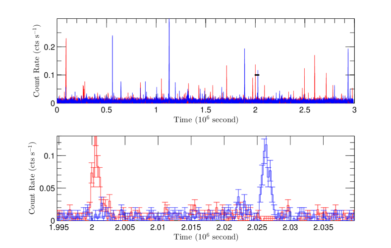
Figure 1.— Upper panel: The light curve (with the observing gaps removed) from the XVP observations (red), compared with a representative one from the simulations (blue) using the best-fit parameters of model I shown in Table 1 (see below). Lower panel: Zoomed-in light curve of a time window indicated by the short horizontal bar in the upper panel.

Fig. 1 shows a representative simulated light curve (blue), compared with the observational one (red) with the observing gaps removed.

2.3. Statistical Comparison

The synthetic light curve cannot be directly compared to the observational one due to the lack of bin-to-bin correspondence between the two. We need a statistical way to make the comparison. A “first” order statistics is the CR distribution, which reveals the overall magnitude of the variabilities. However, as mentioned above (also noted in Neilsen et al. 2015), the CR distribution contains no information about the flare flux correlation among adjacent bins. This correlation can be independently accounted for by the use of the auto-correlation function, or equivalently the SF for a stationary process (Simonetti et al., 1985; Emmanoulopoulos et al., 2010). We jointly fit the CR distribution and the SF to determine the model parameters.

2.3.1 Count Rate Distribution

With the 300-s bins both for the simulated and observed data, the binning results in $M=9964$ data points for the total exposure window. We construct the CR distribution of the data logarithmically and follow Knuth (2006; see also Witzel et al. 2012) to determine the optimal bin number of the histogram. Considering the histogram as a piecewise-constant model, the relative logarithmic posterior probability (RLPP) for the bin number $m$, given $M$ data points, is

$${\rm RLPP}(m) = M\log m+\log\Gamma\left(\frac{m}{2}\right)-m\log\Gamma\left(\frac{1}{2}\right)$$ (4)

$$- \log\Gamma(M+\frac{m}{2})+\sum^{m}_{l=1}\log\Gamma\left(n_{l}+\frac{1}{2}\right),$$

where $n_{l}$ is the histogram value of the $l$th bin, and $\Gamma(x)$ is the Gamma function. Then the optimal number of bins $\bar{m}$ can be derived through maximizing the above $\rm{RLPP}$. For the observational light curve of Sgr A^⋆, we find $m\sim 14$.

With the above binning, we can now construct $\chi^{2}$ statistics for the CR distribution analysis:

$$\chi^{2}_{\rm CR}=(\textbf{n}_{\rm obs}-\textbf{n}_{\rm sim})^{T}\textbf{C}^{-1}(\textbf{n}_{\rm obs}-\textbf{n}_{\rm sim}),$$ (5)

where the symbol ^T stands for the transpose of the matrix (vector), $\textbf{n}_{\rm obs}$ and $\textbf{n}_{\rm sim}$ are the vectors of the CR histogram values of the observed and simulated data, respectively. The covariance matrix C is calculated according to $N$ Monte Carlo realizations

$$C(i,j)=\frac{1}{N-1}\sum_{k=1}^{N}\left(n_{i}^{k}-\bar{n}_{i}\right)\left(n_{j}^{k}-\bar{n}_{j}\right),$$ (6)

where $\bar{n}_{i}$ is the mean value of the $i$th bin of $N$ realizations. The covariance matrix is involved here to account for the error correlations among different bins due to the correlated flare CRs (Brockwell & Davis 2009, and see discussions of the error estimation in Norberg et al. 2009). If there is no correlation between two histogram bins, $C(i,j)=\delta_{ij}\sigma_{i}^{2}$, Eq. (5) is reduced to the standard definition of $\chi^{2}$. The exact value of $N$, as long as it is sufficiently large, has little effect on the calculation of the covariance matrix. In this work we adopt $N=500$.

2.3.2 Structure Function

Following Emmanoulopoulos et al. (2010) we define the normalized SF as

$$V(\tau)=\frac{\left\langle\left[R(t+\tau)-R(t)\right]^{2}\right\rangle}{S^{2}},$$ (7)

where $R(t)$ is the CR as a function of time $t$, $\tau$ is the time lag, $\left\langle\right\rangle$ represents the average over the whole time range of the light curve, and $S^{2}$ is the variance of the CR

$$S^{2}=\left\langle\left[R(t)-\overline{R(t)}\right]^{2}\right\rangle.$$ (8)

This normalized SF is equivalent to the auto-correlation function as long as the time series is stationary, i.e., $\overline{R(t)}=\overline{R(t+\tau)}=\textrm{const.}$ (Emmanoulopoulos et al., 2010). The SF is especially suitable for the analysis of the data that are unequally sampled with large observational gaps, as is the case here.

Similar to the CR distribution, we build a $\chi^{2}$ statistics to compare the observed and simulated SFs quantitatively. Apart from the correlation among various SFs which needs to be taken into account more seriously compared with the CR distribution, another issue for the standard definition of the $\chi^{2}$ is that the random variable (the SF here) needs to be Gaussian. As shown in Emmanoulopoulos et al. (2010), the logarithm of the SF instead of the SF itself is approximately Gaussian. The $\chi^{2}$ statistics for the SF is thus defined as

$$\chi^{2}_{\rm SF}=(\log\textbf{V}_{\rm obs}-\log\textbf{V}_{\rm sim})^{T}\textbf{C}_{\rm SF}^{-1}(\log\textbf{V}_{\rm obs}-\log\textbf{V}_{\rm sim}),$$ (9)

where the covariance matrix $\textbf{C}_{\rm SF}$ can be calculated the same way as Eq. (6). The number of the SF bins for the fitting procedure is chosen to be the same as that of the CR bins, i.e., $m=14$. Note that the SF becomes a featureless plateau when the time lag is larger than the largest time scale of the flares. Correspondingly, the SF for the 14 bins are calculated between 300 s and $3\times 10^{4}$ s. By minimizing $\chi^{2}=\chi^{2}_{\rm CR}+\chi^{2}_{\rm SF}$ , we test our model and constrain the model parameters.

2.3.3 Model Fitting

We minimize $\chi^{2}=\chi^{2}_{\rm CR}+\chi^{2}_{\rm SF}$, using the MCMC method. It maps out the full posterior probability distributions and correlations of the model parameters. The MCMC code is adapted from the public CosmoMC code (Lewis & Bridle, 2002). The Metropolis-Hastings algorithm (Metropolis et al., 1953; Hastings, 1970), a propose-and-accept process in which the acceptance or rejection of a proposed point in the parameter space depends on the probability ratio between this point and the previous one, is adopted to generate the Markov chains.

3. Results

3.1. Joint Fitting

The parameter $\sigma_{\rm ET}$ in the fittings is chosen to be 0.25 according to Yuan et al. (2015). Fig. 2 shows the best-fit results and $1\sigma$ bands of the CR (upper panel) and the SF (lower panel), compared with the observations. The CR distribution exhibits an exponential distribution, which reflects the Possion background, and a power-law tail which represents the flares. The SF increases with $\tau$, and reaches a plateau of $\tau\sim 5\times 10^{3}$ s, which corresponds to the largest duration of the flares. The profile with a rising trend clearly shows the time scale of the flares of the light curve. When the time lag $\tau$ is much longer than the largest time scale of the variabilities, the normalized SF asymptotically approaches 2, i.e., the plateau in Fig. 2. It should be noted that the SF can be biased when applied to irregularly sampled light curves. In particular, the SF can show spurious breaks at $\Delta t\sim 10^{-1}\Delta T$, where $\Delta T$ is the total exposure time of the light curve (Emmanoulopoulos et al., 2010). However, the break seen here is at a much shorter time scale ($\sim 10^{-3}\Delta T$), and consistent with break time scales seen previously in both the NIR (Meyer et al., 2009; Witzel et al., 2012) and sub-millimeter (Dexter et al., 2014). Both of them suggest that the turnover time is likely an intrinsic characteristic time scale for the X-ray flares.

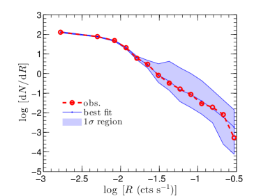
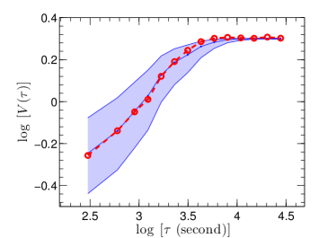
Figure 2.— Upper panel: The CR distribution of the X-ray light curves of Sgr A^⋆. The red circles are for the observed light curve, and blue dots are the best-fit model results. The bands show the fitting $1\sigma$ ranges of the CR distribution for the best-fit model according to the MCMC chains. Lower panel: The SF for the observed data and the simulations for the same parameter set.

Figure 3.— 1D and 2D probability distributions of the fitting parameters. The contours in the 2D plots are for confidence levels $68\%$ and $95\%$ from inside to outside, respectively.

Fig. 3 shows the one and two dimensional (1D and 2D) probability distributions of the parameters. The mean values and the $1\sigma$ uncertainties of the parameters are listed in Table 1. The fitting results suggest a fluence distribution power-law index $\alpha_{\rm E}=1.65\pm 0.17$, and the less constrained fluence-duration correlation index $\alpha_{\rm ET}<0.55~{}$ $(95\%~{}$ confidence limit). The correlations between some of the parameters can be clearly seen in Fig. 3. There is a strong correlation between the total number of flares $\kappa$ and the fluence distribution index $\alpha_{\rm E}$. It is easy to understand that a harder fluence distribution will naturally correspond to a smaller number of flares in order not to over-produce the number of photons. Also the anti-correlation between $\alpha_{\rm E}$ (or $\kappa$) and $r$ is again due to the constraint of the total number of photon counts.

Table 1Best-fit model parameters with the MCMC method

$r\ (10^{-3}~{}\rm{cts~{}s^{-1}})$	$\alpha_{\rm E}$	$\log(\kappa)$	$\log(A)$	$\alpha_{\rm ET}$	$\chi^{2}_{\nu}$
$5.90\pm 0.14$	$1.65\pm 0.17$	$2.41\pm 0.22$	$2.99\pm{0.12}$	$<0.55$	$0.9$

To judge the “goodness of fit” of the best-fit model, we use the bootstrapping method to estimate the confidence level. Based on the best-fit model parameter set as shown in Table 1 we generate 2000 realizations of the light curves and calculate the $\chi^{2}$ values for each realization using the same method described in §2.3. The distribution of the $\chi^{2}$ values is shown in Fig. 4. The number fraction of realizations with $\chi^{2}$ values smaller than that of the observational one, $\chi^{2}_{\rm obs}=21$, is estimated to be $89.7\%$, indicating that the observed light curve is well characterized by the best-fit model.

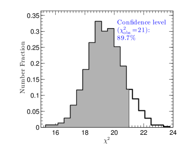
Figure 4.— The distribution of $\chi^{2}$ values of 2000 realizations of the light curves with the best-fit model parameters. The shaded region corresponds to a percentile of $89.7\%$ for $\chi^{2}<\chi^{2}_{\rm obs}$.

Our preliminary re-analysis of the light curve indicates that the existing sample of flares may be biased against the detection of long duration ones. This bias can significantly affect the measurement of $\sigma_{\rm ET}$ and potentially other parameters as well. We have thus tested this latter sensitivity by fixing $\sigma_{\rm ET}$ to different values and find that the estimates of other parameters are not significantly altered (well within their uncertainties). The analysis, however, may be sensitive to the assumed specific shape of individual flares. We will address these potential higher-order complications in a follow-up paper.

3.2. Comparison with previous works

Neilsen et al. (2013) studied the statistical properties of the fluences, peak rates, durations, and luminosities, of the 39 flares detected during the 2012 Chandra XVP. It is found that the distributions of the durations and luminosities can be well described by power-law functions, with indices $\alpha_{\rm T}=0.9\pm 0.2$ and $\alpha_{\rm L}=1.9^{+0.4}_{-0.3}$, respectively. The power-law fittings to the fluence and peak rate distributions give $\alpha_{\rm E}=1.5\pm 0.2$ and $\alpha_{\rm P}=1.9^{+0.5}_{-0.4}$. However, the fittings can be significantly improved by assuming cutoff power-law functions (Neilsen et al., 2013). Our result of $\alpha_{\rm E}$ are consistent with that derived in Neilsen et al. (2013), even though only the detected sample was employed in the latter. Based on the Gaussian flare profile assumption, the slopes of the duration and peak rate distributions can be derived according to our fitting results, which are $\alpha_{\rm T}\gtrsim 2.1$ and $1.7\lesssim\alpha_{\rm P}\lesssim 2.4$, respectively. The peak rate distribution is consistent with that of Neilsen et al. (2013), but the duration distribution is different. As mentioned above, the fluence-duration correlation derived in our work is also different from that of the detected sample. Possible reasons for these discrepancies include the incompleteness of the sample, and the profiles of the flares. Neilsen et al. (2015) showed that the flux distribution can be decomposed into two components, a steady Poisson background and a variable flare component. The X-ray flares excess follows a power-law process with $\alpha_{\rm F}=1.92^{+0.03}_{-0.02}$ and the Poisson background rate is $(5.24\pm 0.08)\times 10^{-3}~{}$cts s^-1. The background rate derived here $(5.90\pm 0.14)\times 10^{-3}~{}$cts s^-1 is slightly larger than that derived in Neilsen et al. (2015), possibly due to the different methods adopted. Although not shown explicitly, our result of Fig. 2 gives roughly $\alpha_{\rm F}\sim 2.2$ which is consistent with that of Neilsen et al. (2015). Wang et al. (2015) also analyzed the detected sample of Neilsen et al. (2013), with different selection of the fitting data ranges, and gave that $\alpha_{\rm E}=1.8\pm 0.6$ and $\alpha_{\rm T}=1.9\pm 0.5$. Within the large uncertainties, their results are consistent with what we obtain.

4. Implications on the nature of the flares

4.1. Confronting the Statistical Results with SOC theory

We find that both the flare fluence distribution and the correlation between the duration and the fluence can be described by power-laws, which is consistent with the prediction of the fractal-diffusive SOC theory (Aschwanden, 2011, 2012, 2014). The SOC theory further predicts that the power-law indices will depend on the Euclidean space dimension $S$ of the system to produce flares. The predicted power-law indices are $\alpha_{\rm E}^{\rm th}\approx 1.5$ and $\alpha_{\rm ET}^{\rm th}\approx 0.5$, respectively, for $S=3$, the classical diffusion parameter $\beta=1$ and the mean fractal dimension $D_{\rm S}=(1+S)/2$ (see the Appendix for more details). These values may vary in a range for different assumed values of $\beta$ and $D_{\rm S}$. For example, $\alpha_{\rm E}$ can range from 1.4 to 1.7 for the fractal dimension $1\leq D_{\rm S=3}\leq 3$. Our results of $\alpha_{\rm E}$ and $\alpha_{\rm ET}$ are actually in good agreement with the theoretical expectation with $S=3$. The predicted indices of the duration and peak rate distributions are $\alpha_{\rm T}^{\rm th}\approx 2.0$ and $\alpha_{\rm P}^{\rm th}\approx 1.7$. As a comparison, our induced values are $\alpha_{\rm T}\gtrsim 2.1$ and $1.7\lesssim\alpha_{\rm P}\lesssim 2.4$, respectively. There are potential discrepancies of these two distributions. Since the determination of the peak rate depends on the assumption of the flare profile, as well as the precise measurement of the flare duration, there should be relatively large uncertainty of the peak CR distribution. As shown in Nowak et al. (2012), the profile, at least for the bright ones, is indeed asymmetric rather than Gaussian. Therefore, the integral property (fluence) should be more reliably measured and more suitable to be used to compare with the theoretical model expectation.

4.2. Episodic ejection of plasma blobs as origin of flares?

Two main conclusions can thus be obtained from the above analysis. First, the power-law distributions of the fluences, durations, and their correlation, suggest that the flares of Sgr A^⋆ can be explained in the fractal-diffusive SOC framework. Second, the inferred space dimension responsible for the flares is $S=3$. Both results are similar to the solar flares, which thus implies that the X-ray flares of Sgr A^⋆ are likely driven by the similar physical mechanism as that of the solar flares. By analogy with the coronal mass ejections and their solar flares, Yuan et al. (2009) have proposed a magnetic reconnection model for the episodic ejections and the production of flares from the accretion flow of Sgr A^⋆. In the following, we briefly review the key points of the model.

The structure of the accretion flow of Sgr A^⋆ is quite similar to the atmosphere of the Sun, i.e., a dense disk enveloped by a tenuous corona, as shown by the magneto-hydrodynamic simulations (e.g., Fig. 4 in Yuan & Narayan, 2014). The magnetic loops emerge into the disk corona due to the Parker instability. The configuration of the coronal magnetic field emerging from the accretion flow is controlled by the convective turbulence motion of the plasma in the disk. Since the foot points of the field lines are anchored in the accretion flow which is turbulent and differentially rotating, a swamp of small-scale magnetic reconnection sets in, which redistributes the helicity and stores most of it in a flux rope. The turbulent processes in the accretion flow thus continuously build up magnetic stress and helicity. When a threshold is reached, e.g., when the current density inside the current sheet below the flux rope is strong enough, microscopic instabilities such as the two-streaming instability would be triggered, resulting in anomalous resistivity and fast magnetic reconnection inside the current sheet (Chen, 2011). The equilibrium of the flux rope breaks down with accompanied dissipation of magnetic energy in a catastrophic manner, powering the observed flare. This is the so-called much-awaited SOC state which means that a small perturbation, owing to turbulence motion in accretion flow and subsequent magnetic reconnection, will trigger an avalanche-like chain reaction of any size in the system once the system self-organizes to a critical state.

5. Conclusions and Discussion

We present a statistical analysis to the Chandra $2-8$ keV X-ray light curve of Sgr A^⋆ from the 3 Ms XVP campaign. A Monte Carlo simulation method is adopted to generate the model light curves taking into account for the Possion fluctuations of both the photon counts and the number of flares. Then we fit the CR distribution and the SF of the light curves jointly to constrain the model parameters, via an MCMC method. We find that the X-ray emission of Sgr A^⋆ can be well modelled by two distinct components: a steady quiescent emission around the Bondi radius with a CR of $(5.90\pm 0.14)\times 10^{-3}~{}\rm{cts\ s}^{-1}$, and a flaring emission with a power-law fluence distribution $dN/dE\propto E^{-\alpha_{\rm E}}$ with $\alpha_{\rm E}=1.65\pm 0.17$. The duration-fluence correlation can also be modelled by a power-law form $T\propto E^{\alpha_{\rm ET}}$ with $\alpha_{\rm ET}<0.55$.

These statistical properties are consistent with the theoretical predications of the SOC system with the Euclid spatial dimension $S=3$, same as that for solar flares (Aschwanden, 2012, 2014). Our analysis, therefore, indicates that the X-ray flares of Sgr A^⋆ are possibly driven by the same physical mechanism as that of the solar flares, i.e., magnetic reconnection (Shibata & Magara, 2011). This idea is further supported by the recent development of magneto-hydrodynamic simulations which lead to the consensus that the accretion flow in Sgr A^⋆ is enveloped by a tenuous corona above the dense disc (e.g., Yuan & Narayan, 2014), similar to the atmosphere of the Sun. The three dimensional geometry of the energy dissipation domain further suggests that the X-ray flaring of Sgr A^⋆ occurs in the surface of the accretion flow due to the less-ordered magnetic field structure embedded in it compared with that in the relativistic astrophysical jets (e.g., the GRBs; Wang & Dai, 2013).

The flares of Sgr A^⋆ have also been detected in the NIR band (e.g., Genzel et al., 2003; Ghez et al., 2004). Dodds-Eden et al. (2011) and Witzel et al. (2012) have analysed the NIR flare data and found that the NIR flux distribution can also be described by a power-law form. However, the power-law indices obtained, which are $-2.1\pm 0.6$ (Dodds-Eden et al., 2011) and $-4.2\pm 0.1$ (Witzel et al., 2012), are different from each other. The cause for this discrepancy between these two results is unclear, and may be related to the subtractions of the stellar light. The former is roughly consistent with that of the X-ray flares (e.g., Neilsen et al., 2015, as well as our results in the context of the SOC framework with $S=3$). If this is the case, then the NIR flares are expected to have the same physical origin as the X-ray flares, which is also supported by the results that NIR and X-ray flares occur simultaneously when there are coordinated observations at two wavebands (e.g., Dodds-Eden et al., 2009). Otherwise, it may suggest different radiation mechanisms between the NIR and X-ray flares which lead to the differences in the fractal dimension (Aschwanden, 2011) or even different physical origins (Chan et al., 2015).

By analogy with solar flares, the multi-waveband flares of Sgr A^⋆ in X-ray, probably NIR, and less prominent sub-millimeter and radio, are likely associated with the ejection of plasmoids, both of which are the radiative manifestation of the common catastrophic phenomena (Yusef-Zadeh et al., 2006, 2008; Brinkerink et al., 2015). Such a result would be useful for understanding the origins of the flares and episodic jets in various black holes in general.

Mineshige et al. (1994b; see also Negoro et al. 1995; Takeuchi et al. 1995) studied the statistical properties of the X-ray fluctuations in Cygnus X-1, a black hole X-ray binary. They found that the X-ray fluctuations showed much steeper (or even exponential) distributions compared with those of solar flares. They argued that the fluctuations should also follow an SOC process. A mass diffusion process was invoked in their works to explain the discrepancy of the distributions. But the X-ray fluctuations they discussed likely have a different physical origin compared with what we have discussed in the present paper. Thus the trigger mechanism of SOC is also different.

Appendix A Self-Organized Criticality System

The theoretical concept of SOC, proposed first by Katz (1986) and Bak et al. (1987) independently, describes a class of nonlinear dissipative dynamical systems which are slowly and continuously driven toward a critical value of an instability threshold, producing scale-free, fractal-diffusive, and intermittent avalanches (Charbonneau et al., 2001; Aschwanden, 2011). The classical example of the SOC system is a sandpile (Bak et al., 1987). If one continuously drops the sand grains (driving force) to the same place, a conical sandpile will grow in a steady way until the surface shape reaches a critical slope, beyond which further addition of sand rapidly leads to catastrophic avalanches of the sandpile. The critical slope is primarily determined by the friction threshold between adjacent grains. Such a threshold is crucial since it allows the existence of multiple metastable states across the system. The continuous slow addition of sand will produce small or large avalanches with sizes independent of the input rate of sand. The critical behavior of the sandpile appears naturally as a consequence of the slow addtion of sand without fine tuning of the addition rate. It is in this sense that the system is self-organized to criticality (Charbonneau et al., 2001; Aschwanden, 2011). The continuous energy input (addition of sand) and nonlinear energy dissipation (avalanches due to the complicated interactions between the colliding sand grains) are two key points to determine whether a system is in an SOC state.

A universal property of the SOC system is that there is no preferred scale of the release of energy. The scale-free power-law distributions of various event parameters, which actually become the hallmarks of SOC systems, are expected. The ubiquitousness of power-law distributions in a wide range of physical systems, e.g., earthquakes, cloud formation, solar flares, and widely in astrophysics, suggests that SOC is a common law of the nature. The SOC theory has been widely applied in geophysics (Turcotte, 1999), solar physics (e.g., Charbonneau et al., 2001), and astrophysics (e.g., Mineshige et al., 1994a; Kawaguchi et al., 2000; Aschwanden, 2011; Kunjaya et al., 2011).

The slope of the power-law form depends on how the subsystem self-organizes to the critical state. An analytic description was provided based on a fractal-diffusive avalanche model (Aschwanden, 2012). The SOC state ensures that the entire system is close to the instability threshold, and the avalanches can develop in any direction once triggered. The propagation of the unstable nodes can thus be modelled with a random walk in an $S$-dimensional space (Aschwanden, 2012). A statistical correlation between the spatial length scale $L$ and time duration of the avalanche $T$ for a diffusive random walk is predicted to be $L\propto{T}^{\beta/2}$, where $\beta$ is a diffusion parameter ($\beta=1$ corresponds to the classical diffusion). With the scale-free probability conjection $dN/dL\propto{L}^{-\rm S}$, which means that the critical states are homegeneously distributed across the entire system, the occurrence frequency distributions of flare duration, flux, peak flux, and total energy can be obtained in the fractal-diffusive avalanche model (Aschwanden, 2012). The indices of the total energy (fluence) $\alpha_{\rm E}^{\rm th}$, duration $\alpha_{\rm T}^{\rm th}$, peak luminosity (or peak CR in this work) $\alpha_{\rm P}^{\rm th}$, and flux (or CR) $\alpha_{\rm F}^{\rm th}$ distributions are derived as (Aschwanden, 2012, 2014)

$$\alpha_{\rm E}^{\rm th} = 1+\frac{S-1}{D_{\rm S}+2/\beta},$$ (A1)

$$\alpha_{\rm T}^{\rm th} = 1+\frac{(S-1)\beta}{2},$$ (A2)

$$\alpha_{\rm P}^{\rm th} = 1+\frac{S-1}{S},$$ (A3)

$$\alpha_{\rm F}^{\rm th} = 1+\frac{S-1}{D_{\rm S}},$$ (A4)

where $S$ is the Euclidean space dimension, $D_{\rm S}$ is the fractal Hausdorff dimension which lies between 1 and $S$. The fractal-diffusive SOC theory also predicts the scaling relations between various flare parameters. The correlation slope between the total energy $E$ and duration $T$ is (Aschwanden, 2012, 2014)

$$\alpha_{\rm ET}^{\rm th}=\frac{2}{D_{\rm S}\beta+2}.$$ (A5)

For the classical diffusion $(\beta=1)$ and an estimated mean fractal dimension of $D_{\rm S}\approx(S+1)/2$, we have $\alpha_{\rm E}^{\rm th}=1.5$, $\alpha_{\rm T}^{\rm th}=2.0$, $\alpha_{\rm P}^{\rm th}=1.7$, $\alpha_{\rm F}^{\rm th}=2.0$, and $\alpha_{\rm ET}^{\rm th}=0.5$ for $S=3$.

References

- Aharonian et al. (2008) Aharonian, F., Akhperjanian, A. G., Barres de Almeida, U., et al. 2008, A&A, 492, L25
- Aschwanden (2012) Aschwanden, M. J. 2012, A&A, 539, A2
- Aschwanden (2014) Aschwanden, M. J. 2014, ApJ, 782, 54
- Aschwanden (2011) Aschwanden, M. J. 2011, Self-Organized Criticality in Astrophysics, by Markus J. Aschwanden. Springer-Praxis, Berlin ISBN 978-3-642-15000-5, 416p.
- Aschwanden & McTiernan (2010) Aschwanden, M. J., & McTiernan, J. M. 2010, ApJ, 717, 683
- Baganoff et al. (2001) Baganoff, F. K., Bautz, M. W., Brandt, W. N., et al. 2001, Nature, 413, 45
- Baganoff et al. (2003) Baganoff, F. K., Maeda, Y., Morris, M., et al. 2003, ApJ, 591, 891
- Bak et al. (1987) Bak, P., Tang, C., & Wiesenfeld, K. 1987, Physical Review Letters, 59, 381
- Barrière et al. (2014) Barrière, N. M., Tomsick, J. A., Baganoff, F. K., et al. 2014, ApJ, 786, 46
- Bélanger et al. (2005) Bélanger, G., Goldwurm, A., Melia, F., et al. 2005, ApJ, 635, 1095
- Brinkerink et al. (2015) Brinkerink, C. D., Falcke, H., Law, C. J., et al. 2015, A&A, 576, A41
- Broderick & Loeb (2005) Broderick, A. E., & Loeb, A. 2005, MNRAS, 363, 353
- Brockwell & Davis (2009) Brockwell, P. J. & Davis, R. A. 2010, Introduction to time series and forecasting, by Peter J. Brockwell and Richard A. Davis.2nd ed. Springer Series in Statistics. New York: Springer-Verlag, 2002.
- Chan et al. (2015) Chan, C.-K., Psaltis, D., Ozel, F., et al. 2015, arXiv:1505.01500
- Charbonneau et al. (2001) Charbonneau, P., McIntosh, S. W., Liu, H.-L., & Bogdan, T. J. 2001, Sol. Phys., 203, 321
- Chen (2011) Chen, P. F. 2011, Living Reviews in Solar Physics, 8, 1
- Degenaar et al. (2013) Degenaar, N., Miller, J. M., Kennea, J., et al. 2013, ApJ, 769, 155
- Dexter et al. (2014) Dexter, J., Kelly, B., Bower, G. C., et al. 2014, MNRAS, 442, 2797
- Dodds-Eden et al. (2011) Dodds-Eden, K., Gillessen, S., Fritz, T. K., et al. 2011, ApJ, 728, 37
- Dodds-Eden et al. (2009) Dodds-Eden, K., Porquet, D., Trap, G., et al. 2009, ApJ, 698, 676
- Dodds-Eden et al. (2010) Dodds-Eden, K., Sharma, P., Quataert, E., et al. 2010, ApJ, 725, 450
- Eckart et al. (2006) Eckart, A., Baganoff, F. K., Schödel, R., et al. 2006, A&A, 450, 535
- Emmanoulopoulos et al. (2010) Emmanoulopoulos, D., McHardy, I. M., & Uttley, P. 2010, MNRAS, 404, 931
- Genzel et al. (2003) Genzel, R., Schödel, R., Ott, T., et al. 2003, Nature, 425, 934
- Genzel et al. (2010) Genzel, R., Eisenhauer, F., & Gillessen, S. 2010, Reviews of Modern Physics, 82, 3121
- Ghez et al. (2004) Ghez, A. M., Wright, S. A., Matthews, K., et al. 2004, ApJ, 601, L159
- Hastings (1970) Hastings, W.K., 1970, Biometrika, 57, 97
- Katz (1986) Katz, J. I. 1986, J. Geophys. Res., 91, 10412
- Kawaguchi et al. (2000) Kawaguchi, T., Mineshige, S., Machida, M., Matsumoto, R., & Shibata, K. 2000, PASJ, 52, L1
- Knuth (2006) Knuth, K. H. 2006, arXiv:physics/0605197
- Kunjaya et al. (2011) Kunjaya, C., Mahasena, P., Vierdayanti, K., & Herlie, S. 2011, Ap&SS, 336, 455
- Lewis & Bridle (2002) Lewis, A., & Bridle, S. 2002, Phys. Rev. D, 66, 103511
- Li et al. (2013) Li, J., Ostriker, J. P., & Sunyaev, R. 2013, ApJ, 767, 105
- Lin & Forbes (2000) Lin, J., & Forbes, T. G. 2000, J. Geophys. Res., 105, 2375
- Lu & Hamilton (1991) Lu, E. T., & Hamilton, R. J. 1991, ApJ, 380, L89
- Markoff et al. (2001) Markoff, S., Falcke, H., Yuan, F., & Biermann, P. L. 2001, A&A, 379, L13
- Marrone et al. (2008) Marrone, D. P., Baganoff, F. K., Morris, M. R., et al. 2008, ApJ, 682, 373
- Metropolis et al. (1953) Metropolis, N., Rosenbluth, A.W., Rosenbluth, M.N., Teller, A.H., Teller, E. 1953, J. Chem. Phys., 21, 1087M
- Meyer et al. (2009) Meyer, L., Do, T., Ghez, A., et al. 2009, ApJ, 694, L87
- Mineshige et al. (1994a) Mineshige, S., Ouchi, N. B., & Nishimori, H. 1994a, PASJ, 46, 97
- Mineshige et al. (1994b) Mineshige, S., Takeuchi, M., & Nishimori, H. 1994b, ApJ, 435, L125
- Narayan et al. (2012) Narayan, R., SÄ dowski, A., Penna, R. F., & Kulkarni, A. K. 2012, MNRAS, 426, 3241
- Negoro et al. (1995) Negoro, H., Kitamoto, S., Takeuchi, M., & Mineshige, S. 1995, ApJ, 452, L49
- Neilsen et al. (2013) Neilsen, J., Nowak, M. A., Gammie, C., et al. 2013, ApJ, 774, 42
- Neilsen et al. (2015) Neilsen, J., Markoff, S., Nowak, M. A., et al. 2015, ApJ, 799, 199
- Norberg et al. (2009) Norberg, P., Baugh, C. M., Gaztañaga, E., & Croton, D. J. 2009, MNRAS, 396, 19
- Nowak et al. (2012) Nowak, M. A., Neilsen, J., Markoff, S. B., et al. 2012, ApJ, 759, 95
- Porquet et al. (2008) Porquet, D., Grosso, N., Predehl, P., et al. 2008, A&A, 488, 549
- Porquet et al. (2003) Porquet, D., Predehl, P., Aschenbach, B., et al. 2003, A&A, 407, L17
- Priest & Forbes (2000) Priest, E., & Forbes, T. 2000, Magnetic reconnection : MHD theory and applications New York : Cambridge University Press, 2000.
- Shibata & Magara (2011) Shibata, K., & Magara, T. 2011, Living Reviews in Solar Physics, 8, 6
- Simonetti et al. (1985) Simonetti, J. H., Cordes, J. M. & Heeschen, D. S. 1985, ApJ, 296, 46
- Tagger & Melia (2006) Tagger, M., & Melia, F. 2006, ApJ, 636, L33
- Takeuchi et al. (1995) Takeuchi, M., Mineshige, S., & Negoro, H. 1995, PASJ, 47, 617
- Trap et al. (2011) Trap, G., Goldwurm, A., Dodds-Eden, K., et al. 2011, A&A, 528, A140
- Turcotte (1999) Turcotte, D. L. 1999, Rep. Prog. Phys., 62, 1377
- Wang & Dai (2013) Wang, F. Y., & Dai, Z. G. 2013, Nature Physics, 9, 465
- Wang et al. (2015) Wang, F. Y., Dai, Z. G., Yi, S. X., & Xi, S. Q. 2015, ApJS, 216, 8
- Wang (2004) Wang, Q. D. 2004, ApJ, 612, 159
- Wang et al. (2013) Wang, Q. D., Nowak, M. A., Markoff, S. B., et al. 2013, Science, 341, 981
- Witzel et al. (2012) Witzel, G., Eckart, A., Bremer, M., et al. 2012, ApJS, 203, 18
- Yuan et al. (2012) Yuan, F., Bu, D., & Wu, M. 2012, ApJ, 761, 130
- Yuan et al. (2009) Yuan, F., Lin, J., Wu, K., & Ho, L. C. 2009, MNRAS, 395, 2183
- Yuan & Narayan (2014) Yuan, F., & Narayan, R. 2014, ARA&A, 52, 529
- Yuan et al. (2004) Yuan, F., Quataert, E., & Narayan, R. 2004, ApJ, 606, 894
- Yuan et al. (2003) Yuan, F., Quataert, E., & Narayan, R. 2003, ApJ, 598, 301
- Yuan et al. (2015) Yuan, Q., et al. 2015, in preparation
- Yusef-Zadeh et al. (2006) Yusef-Zadeh, F., Roberts, D., Wardle, M., Heinke, C. O., & Bower, G. C. 2006, ApJ, 650, 189
- Yusef-Zadeh et al. (2008) Yusef-Zadeh, F., Wardle, M., Heinke, C., et al. 2008, ApJ, 682, 361
- Yusef-Zadeh et al. (2009) Yusef-Zadeh, F., Bushouse, H., Wardle, M., et al. 2009, ApJ, 706, 348
- Zubovas et al. (2012) Zubovas, K., Nayakshin, S., & Markoff, S. 2012, MNRAS, 421, 1315