Overapproximating the Reachable Values Set of Piecewise Affine Systems Coupling Policy Iterations with Piecewise Quadratic Lyapunov Functions

Abstract

We have recently constructed a piecewise quadratic Lyapunov function to prove the boundedness of the reachable values set of piecewise affine discrete-time systems. The method developed also provided an overapproximation of the reachable values set. In this paper, we refine the latter overapproximation extending previous works combining policy iterations with quadratic Lyapunov functions.

1 Introduction

Several catastrophic events showed the importance of the formal verification of programs. Some of these failures are caused by overflows. A method to prove the absence of overflows in numerical programs consists in providing precise safe bounds over the reachable states of the program variables.

In this paper, we are interesting in a particular class of numerical programs: single while loop programs with a switch-case structure inside the loop body. Moreover, we suppose that test and assignment functions are affine. These programs can be represented as piecewise affine discrete-time systems. To overapproximate the reachable states of the program variables is thus reduced to overapproximate the reachable values set of a piecewise affine discrete-time system. Hence, we propose to compute automatically precise bounds over piecewise affine discrete-time systems using policy iterations and piecewise quadratic Lyapunov functions.

Initially policy iteration solves stochastic control problems [How60] which can be reduced to solve fixed point problems involving functions with maxima of affine functions coordinates. Policy iteration was then extended to zero-sum two-player stochastic games [HK66], this extension allows the computation of the unique fixed point of min-max of affine maps. The very first extension of policy iterations in program analysis was in 2005 by Costan et al [CGG⁺05]. Since then, the usage of policy iteration in various verification problems greatly increases: in [GSA⁺12], the authors describe policy iteration algorithm to overapproximate the reachable values set of numerical programs with affine assignments; in [Mas12], the author proves termination by policy iteration; in [SS13, SJVG11] the authors propose to embed policy iterations for programs dealing with both numerical and boolean variables.

The method developed in [AG15] allows to prove that the reachable values set of a piecewise affine system is bounded. The method relies on the synthesis of a piecewise quadratic Lyapunov function of this piecewise affine system. The problem formulation makes appear as a decision variable an upper bound on the Euclidian norm of the state variable. This upper bound can be very loose since it combines all the coordinates together. We propose to use a templates based method. A templates method consists in representing sets as sublevel sets of given functions called templates. Then to compute an overapproximation is reduced to computing bounds over the templates. The most precise overapproximation with respect to these templates is provided by the vector of bounds satisfying a smallest fixed point. In our context, the generated piecewise quadratic Lyapunov function is used as a template. We complete the templates basis by the square of variables. Finally we use policy iterations to solve the (smallest) fixed point equation. Thus, policy iterations algorithm leads to tighter bounds over the reachable values set.

The use of quadratic Lyapunov function as quadratic templates was explicitly done in [RJGF12] but it is not enough to prove the boundedness of reachable values set of a piecewise affine system unless that a common quadratic Lyapunov function exists. Policy iteration algorithms in templates domain proposed in [AGG12, GSA⁺12] used quadratic templates and did not handle piecewise quadratic templates. In this paper, we adapt policy iteration based on Lagrange duality [Adj14] to piecewise quadratic functions. The works on piecewise quadratic Lyapunov functions [Joh03, MFTM00] are also related to this paper. Their authors are interested in proving stability of piecewise linear systems. However, as classical quadratic Lyapunov functions, piecewise quadratic Lyapunov functions provide sublevel invariant sets to the system. We use this latter interpretation for a verification purpose. Finally, note that tropical polyhedra domain [All09] generates disjunctions of zones as invariants. The latter invariants did not encode quadratic relations between variables.

The first contribution of the paper is the formalisation of piecewise quadratic Lyapunov functions to prove the boundedness of the trajectories of a piecewise affine discrete-time dynamical system. This formalisation uses the theory of cone-copositive matrices which is also an original contribution in this context.

The main contribution of the article is the extension of policy iterations algorithm to the piecewise quadratic Lyapunov functions in order to provide precise bounds on the reachable values. Indeed, policy iteration has just been constructed in the case of quadratic functions.

Notations

Numbers. $\mathbb{N}$ denotes the set of nonnegative integers, then for $d\in\mathbb{N}$, $[d]=\{1,\ldots,d\}$. $\mathbb{R}$ is the set of reals, $\mathbb{R}_{+}$ the set of nonnegative reals and $\mathbb{R}^{d}$ denotes the set of vectors of $d$ reals. We denote by $\wp(\mathbb{R}^{d})$ the set of subsets of $\mathbb{R}^{d}$.

Inequalities. For $y,z\in\mathbb{R}^{d}$, $y<z$ (resp. $y\leq z$) means $\forall\,l\in[d]$, $y_{l}<z_{l}$, (resp. $\forall\,l\in[d]$, $y_{l}\leq z_{l}$) and $y\leq_{w,s}z$ is a mix of weak and strict inequalities.

Matrices. $\mathbb{M}_{n\times m}$ is the set of matrices with $n$ rows and $m$ columns. $0_{n,m}$ and $0_{n}$ are respectively the null matrices of $\mathbb{M}_{n\times m}$ and $\mathbb{M}_{n\times n}$. $\operatorname{Id}_{n}$ is the identity matrix of $\mathbb{M}_{n\times n}$. $M^{\intercal}$ is the transpose of $M\in\mathbb{M}_{n\times m}$. $\mathbb{S}_{n}$ is the set of symmetric matrices of size $n\times n$. $A\succeq 0$ means that $A$ is semi-definite positive i.e. $A\in\mathbb{S}_{d}$ and $\forall\,x\in\mathbb{R}^{d}$, $x^{\intercal}Ax\geq 0$. $\mathbb{S}_{d}^{+}$ is the convex cone of semidefinite positive matrices.

2 Piecewise affine discrete-time systems

In this section, we detail the systems we will consider in the paper.

Piecewise affine systems (PWA for short) are defined as systems the dynamic of which is piecewise affine and thus the dynamic is characterized by a polyhedral partition and a family of affine maps relative to this partition. For us, a polyhedral partition is a family of convex polyhedra such that:

$$\bigcup_{i\in\mathcal{I}}X^{i}=\mathbb{R}^{d}\text{ and }\forall\,i,j\in\mathcal{I},\ i\neq j\ X^{i}\cap X^{j}=\emptyset\enspace.$$ (1)

The convex polyhedron $X^{i}$ can contain both strict and weak inequalities and is represented by $T^{i}\in\mathbb{M}_{n_{i}\times m}$ and $c^{i}\in\mathbb{R}^{n_{i}}$. We denote by $T_{s}^{i}$ (resp. $T_{w}^{i}$) and $c_{s}^{i}$ (resp. $c_{w}^{i}$) the parts of $T^{i}$ and $c^{i}$ corresponding to strict (resp. weak) inequalities:

$$\begin{array}[]{ll}X^{i}&=\left\{x\in\mathbb{R}^{d}\left|T^{i}x\leq_{w,s}c^{i}\right\}\right.\\ &=\left\{x\in\mathbb{R}^{d}\left|T_{s}^{i}x<c_{s}^{i},\ T_{w}^{i}x\leq c_{w}^{i}\right\}\right.\end{array}$$ (2)

Definition 1 (Piecewise Affine System)

A PWA is characterized by the triple $(X^{0},\mathcal{X},\mathcal{A})$ where:

• $X^{0}$ is the polytope of the initial conditions of the form (2);

• $\mathcal{X}:=\{X^{i},i\in\mathcal{I}\}$ is a polyhedral partition i.e. satisfying (1);

• $\mathcal{A}:=\{x\mapsto f^{i}(x)=A^{i}x+b^{i},i\in\mathcal{I}\}$ where $A^{i}\in\mathbb{M}_{d\times d}$ and $b^{i}\in\mathbb{R}^{d}$;

And satisfies the following relation for all $k\in\mathbb{N}$:

$$x_{0}\in X^{0},\ \text{if }x_{k}\in X^{i},\ x_{k+1}=f^{i}(x_{k})\enspace.$$ (3)

Let $P=(X^{0},\mathcal{X},\mathcal{A})$ be a PWA. We now define some tools that we need during the analysis. First we define the reachable values set $\mathcal{R}$ of $P$:

$$\mathcal{R}=\bigcup_{k\in\mathbb{N}}{\mathbb{A}}^{k}(X^{0}),\text{ where }\mathbb{A}(x)=f^{i}(x)\text{ if }x\in X^{i}$$ (4)

We define the set of possible switches:

$$\begin{array}[]{l}\mathrm{Sw}:=\{(i,j)\in\mathcal{I}^{2}\mid\mathcal{R}\cap X^{ij}\neq\emptyset\}\\ \text{ where }X^{ij}=X^{i}\cap{f^{i}}^{-1}(X^{j})\enspace.\end{array}$$ (5)

Finally, we define the set of indices of polyhedra of $\mathcal{X}$ which meet the polyhedron of possible initial conditions:

$$\mathrm{In}:=\{i\in\mathcal{I}\mid X^{i0}\neq\emptyset\}\text{ where }X^{i0}=X^{i}\cap X^{0}\enspace.$$ (6)

We introduce for $i\in\mathcal{I}$, the following matrix of $\mathbb{M}_{(d+1)\times(d+1)}$:

$$F^{i}=\begin{pmatrix}1&0_{1\times d}\\ b^{i}&A^{i}\end{pmatrix}\enspace.$$ (7)

Eq. (3) can be rewritten as $(1,x_{k+1})^{\intercal}=F^{i}(1,x_{k})$.

We are interested in computing automatically precise overapproximation of $\mathcal{R}$. We propose to compute an overapproximation of $\mathcal{R}$ as a set $S\subseteq\mathbb{R}^{d}$ such that $X^{0}\subseteq S$ and $\forall\,i\in\mathcal{I},\ x\in S\cap X^{i}\implies A^{i}x+b^{i}\in S$. The set $S$ can be computed as a sublevel of a Lyapunov function containing the initial states.

From now, we work with a fixed PWA $P=(X^{0},\mathcal{X},\mathcal{A})$, where $X^{0}$, $\mathcal{X}$ and $\mathcal{A}$ are of the form of Def. 1.

3 Piecewise quadratic Lyapunov functions

In this paper, we use piececewise quadratic Lyapunov functions for piecewise affine systems to compute directly an overapproximation of reachable values set.

Let $q$ be a quadratic form i.e. a function such that for all $y\in\mathbb{R}^{d}$, $q(y)=y^{\intercal}A_{q}y+b_{q}^{\intercal}y+c_{q}$ where $A_{q}\in\mathbb{S}_{d}$, $b_{q}\in\mathbb{R}^{d}$ and $c_{q}\in\mathbb{R}$. We define the lift-matrix of $q$, the matrix of $\mathbb{S}_{d+1}$ defined as follows:

$$\mathbf{M}(A_{q},b_{q},c_{q})=\mathbf{M}(q)=\begin{pmatrix}c_{q}&(b_{q}/2)^{\intercal}\\ (b_{q}/2)&A_{q}\end{pmatrix}$$ (8)

It is obvious that the $q\mapsto\mathbf{M}(q)$ is linear. Let $A\in\mathbb{M}_{d\times d}$, $b\in\mathbb{R}^{d}$, and $q$ be a quadratic form, we have, for all $x\in\mathbb{R}^{d}$:

$$q(Ax+b)=\begin{pmatrix}1\\ x\end{pmatrix}^{\intercal}\begin{pmatrix}1&0_{1\times d}\\ b&A\end{pmatrix}^{\intercal}\mathbf{M}(q)\begin{pmatrix}1&0_{1\times d}\\ b&A\end{pmatrix}\begin{pmatrix}1\\ x\end{pmatrix}\enspace.$$ (9)

Lemma 1

Let $A\in\mathbb{S}_{d}$, $b\in\mathbb{R}^{d}$ and $c\in\mathbb{R}$. Then: $(\forall\,y\in\mathbb{R}^{d},\ y^{\intercal}Ay+b^{\intercal}y+c\geq 0)\iff\mathbf{M}(A,b,c)\in\mathbb{S}_{d+1}^{+}$

Definition 2 ((Cone)-copositive matrices)

Let $M\in\mathbb{M}_{m\times d}$. A matrix $Q\in\mathbb{S}_{d}$ which satisfies

$$My\geq 0\implies y^{\intercal}Qy\geq 0$$

is called $M$-copositive.

An $\operatorname{Id}_{d}$-copositive matrix is called a copositive matrix. We denote by $\mathbf{C}_{d}\left(M\right)$ the set of $M$-copositive matrices and $\mathbf{C}_{d}$ the set of copositive matrices.

For $P\in\mathbb{M}_{n\times m}$ and $c\in\mathbb{R}^{n}$, we define the following matrix:

$$\overline{\mathbf{H}\left(P,c\right)}=\begin{pmatrix}1&&0_{1\times m}\\ c&&-P\end{pmatrix}\in\mathbb{M}_{(n+1)\times(m+1)}$$ (10)

Lemma 2

Let $P\in\mathbb{M}_{n\times m}$ and $c\in\mathbb{R}^{n}$. Then, for all $x\in\mathbb{R}^{n}$, $Px\leq c\iff\overline{\mathbf{H}\left(P,c\right)}\begin{pmatrix}1\\ x\end{pmatrix}\geq 0$.

Lemma 3

Let $q:\mathbb{R}^{d}\to\mathbb{R}^{d}$ be a quadratic function. Let $M\in\mathbb{M}_{m\times d}$ and $p\in\mathbb{R}^{m}$. Let us consider $C=\{x\mid Mx\leq p\}$. Then $\mathbf{M}(q)\in\mathbf{C}_{d+1}\left(\overline{\mathbf{H}\left(M,p\right)}\right)\implies(q(x)\geq 0,\ \forall\,x\in C)$.

and we introduce the following matrices:

$$\forall\,i\in\mathcal{I},\ E^{i}=\overline{\mathbf{H}\left(T^{i},c^{i}\right)}\enspace,$$ (11a)

$$\forall\,(i,j)\in\mathcal{I}^{2},\ E^{ij}=\overline{\mathbf{H}\left(\begin{pmatrix}T^{i}\\ T^{j}A^{i}\end{pmatrix},\begin{pmatrix}c^{i}\\ c^{j}-T^{j}b^{i}\end{pmatrix}\right)}\enspace,$$ (11b)

$$\forall\,i\in\mathrm{In},\ E^{i0}=\overline{\mathbf{H}\left(\begin{pmatrix}T^{i}\\ T^{0}\end{pmatrix},\begin{pmatrix}c^{i}\\ c^{0}\end{pmatrix}\right)}\enspace.$$ (11c)

Lemma 4

For all $i\in\mathcal{I}$, $X^{i}\subseteq\{x\mid E^{i}(1\ x^{\intercal})^{\intercal}\geq 0\}$, for all $(i,j)\in\mathrm{Sw}$, $X^{ij}\subseteq\{x\mid E^{ij}(1\ x^{\intercal})^{\intercal}\geq 0\}$ and for all $i\in\mathrm{In}$, $X^{i0}\subseteq\{x\mid E^{i0}(1\ x^{\intercal})^{\intercal}\geq 0\}$.

Definition 3 (PQL functions)

A function $L$ is a piecewise quadratic Lyapunov function (PQL for short) for $P$ if and only if there exist a family $\{(P^{i},q^{i}),P^{i}\in\mathbb{S}_{d},q^{i}\in\mathbb{R}^{d},\ i\in\mathcal{I}\}$ and two reals $\alpha$ and $\beta$ such that:

1. $\forall\,i\in\mathcal{I}$, $\forall\,x\in X^{i}$, $L(x)=L^{i}(x)=x^{\intercal}P^{i}x+2x^{\intercal}q^{i}$;

2. $\forall\,i\in\mathcal{I}$:

   $$\mathbf{M}(P^{i},2q^{i},-\alpha)-\mathbf{M}(\operatorname{Id},0,-\beta)\in\mathbf{C}_{d+1}\left(E^{i}\right)\enspace;$$ (12)

3. $\forall\,(i,j)\in\mathrm{Sw}$:

   $$\mathbf{M}(P^{i},2q^{i},0)-{F^{i}}^{\intercal}\mathbf{M}(P^{j},2q^{j},0)F^{i}\in\mathbf{C}_{d+1}\left(E^{ij}\right)\enspace;$$ (13)

4. $\forall\,i\in\mathrm{In}$:

   $$-\mathbf{M}(P^{i},2q^{i},-\alpha)\in\mathbf{C}_{d+1}\left(E^{i0}\right)\enspace.$$ (14)

Theorem 1 (Bounded trajectories)

Assume that $P$ admits a PQL function characterized by $\{(P^{i},q^{i}),P^{i}\in\mathbb{S}_{d},q^{i}\in\mathbb{R}^{d},\ i\in\mathcal{I}\}$ and reals $\alpha$ and $\beta$. Let $i\in\mathcal{I}$, $S_{\alpha}^{i}=\{x\in X^{i}\mid L^{i}(x)\leq\alpha\}=\{x\in X^{i}\mid x^{\intercal}P^{i}x+2x^{\intercal}q^{i}\leq\alpha\}$ and $S=\cup_{i\in\mathcal{I}}S_{\alpha}^{i}$. Then, $\mathcal{R}\subseteq S\subseteq\{x\in\mathbb{R}^{d}\mid\mbox{$\|x\|$}_{2}^{2}\leq\beta\}$.

Proof 1

First, we prove that $S\subseteq\{x\in\mathbb{R}^{d}\mid\mbox{$\|x\|$}_{2}^{2}\leq\beta\}$. Let $i\in\mathcal{I}$ and $x\in X^{i}$. From Eq. (12), Lemma 3 and Lemma 4, $x^{\intercal}P^{i}x+2x^{\intercal}q^{i}-\alpha-\mbox{$\|x\|$}_{2}^{2}+\beta\geq 0$. This is equivalent to $\beta-\mbox{$\|x\|$}_{2}^{2}\geq\alpha-x^{\intercal}P^{i}x-2x^{\intercal}q^{i}$ which implies that $S\subseteq\{x\in\mathbb{R}^{d}\mid\mbox{$\|x\|$}_{2}^{2}\leq\beta\}$.

Now, we have to prove $\mathcal{R}\subseteq S$. From Eq. (4), we have to prove that for all $k\in\mathbb{N}$, $\mathbb{A}^{k}(X^{0})\subseteq S$. We prove it by induction on $k$. Let $x\in X^{0}$. Since $\mathcal{X}$ satisfies (1), there exists a unique $i\in\mathrm{In}$ such that $x_{0}\in X^{i0}$. From Eq. (14), Lemma 3 and Lemma 4, $L^{i}(x)\leq\alpha$. Now suppose $\mathbb{A}^{k}(X^{0})\subseteq S$ for some $k\in\mathbb{N}$. Let $y\in\mathbb{A}^{k+1}(X^{0})$. Then $y=\mathbb{A}(x)$ for some $x\in\mathbb{A}^{k}(X^{0})$. Since $\mathcal{X}$ satisfies (1), there exists an unique $(i,j)\in\mathrm{Sw}$ such that $x\in X^{ij}$ (hence $y\in X^{j}$). As $x\in X^{i}$ and $x\in S$, then $x\in S_{\alpha}^{i}$. From Eq. (13), Lemma 3 and Lemma 4, $0\leq L^{i}(x)-L^{j}(y)=L^{i}(x)-\alpha-(L^{j}(y)-\alpha)$. As $x\in S_{\alpha}^{i}$, $0\geq L^{i}(x)-\alpha$ which implies that $0\geq L^{j}(y)-\alpha$ and finally $y\in S_{\alpha}^{j}\subseteq S$.

3.1 Computational issues

To construct PQL functions, we are faced with two issues. First, we must know the sets of indices $\mathrm{Sw}$ and $\mathrm{In}$. Second we have to manipulate cone-copositive constraints.

3.1.1 The computation of sets $\mathrm{Sw}$ and $\mathrm{In}$

To set $\mathrm{Sw}$ is defined from $\mathcal{R}$, the set which we want approximate. To overcome this issue, we consider a bigger set by removing the intersection with $\mathcal{R}$:

$$\overline{\mathrm{Sw}}:=\{(i,j)\in\mathcal{I}^{2}\mid X^{ij}\neq\emptyset\}\enspace.$$ (15)

Since $X^{i}$ and $X^{j}$ can contain strict inequalities, we can use alternative theorems such as Motzkin’s theorem [Mot51] to compute $\overline{\mathrm{Sw}}$. Note that we use this technique based LP to determine exactly $\mathrm{In}$.

The direct application of Motzkin’s transposition theorem [Mot51] yields to the next proposition.

Proposition 1

Let $n_{ij}^{s}$ (resp. $n_{ij}^{w}$) be the number of strict (resp. weak) inequalities in $X^{i}\cap X^{j}$. The couple $(i,j)\in\overline{\mathrm{Sw}}$ if and only if:

$$\left\{\begin{array}[]{l}\displaystyle{\begin{pmatrix}1&&0_{1\times d}\\ c_{s}^{i}&&-T_{s}^{i}\\ c_{s}^{j}-T_{s}^{j}b^{i}&&-T_{s}^{j}A^{i}\end{pmatrix}^{\intercal}p^{s}+\begin{pmatrix}c_{w}^{i}&&-T_{w}^{i}\\ c_{w}^{j}-T_{w}^{j}b^{i}&&-T_{w}^{j}\end{pmatrix}^{\intercal}p=0}\\ \\ \displaystyle{\sum_{k=1}^{n_{ij}^{s}+1}p_{k}^{s}=1},\ p^{s}\geq 0,\ p\geq 0\end{array}\right.$$

has no solution.

Let $n_{i0}^{s}$ (resp. $n_{i0}^{w}$) be the number of strict (resp. weak) inequalities in $X^{i}\cap X^{0}$. The index $i\in\mathrm{In}$ if and only if:

$$\left\{\begin{array}[]{l}\begin{pmatrix}1&&0_{1\times d}\\ c_{s}^{i}&&-T_{s}^{i}\\ c_{s}^{0}&&-T_{s}^{0}\end{pmatrix}^{\intercal}p^{s}+\begin{pmatrix}c_{w}^{i}&&-T_{w}^{i}\\ c_{w}^{0}&&-T_{w}^{0}\end{pmatrix}^{\intercal}p=0\\ \\ \displaystyle{\sum_{k=1}^{n_{i0}^{s}+1}p_{k}^{s}=1,\ p^{s}\geq 0,\ p\geq 0}\end{array}\right.$$

has no solution.

3.1.2 Cone-copositive constraints

Cone-copositive matrix characterizations is an intensive research field and a list of interesting papers about can be found in [BSU12].

Proposition 2 (Th. 2.1 of [MJ81])

Let $M\in\mathbb{M}_{m\times d}$. Then:

$$\{M^{\intercal}CM+S\mid C\in\mathbf{C}_{d}\text{ and }S\in\mathbb{S}_{d}^{+}\}\subseteq\mathbf{C}_{d}\left(M\right) \Delta$$ ()

If the rank of $M$ is equal to $m$, then ($\Delta$) is actually an equality.

The next proposition discusses simple a characterization of copositive matrices as a sum of a semi-definite positive matrix and a nonnegative matrix.

Proposition 3 ( [Dia62, MM62])

We have: $\forall\,d\in\mathbb{N}$: $\mathbb{S}_{d}^{\geq 0}+\mathbb{S}_{d}^{+}\subseteq\mathbf{C}_{d}$. If $d\leq 4$ then $\mathbf{C}_{d}=\mathbb{S}_{d}^{\geq 0}+\mathbb{S}_{d}^{+}$.

Corollary 1

Let $M\in\mathbb{M}_{m\times d}$. Then:

$$\mathbf{C}_{d}\left(M\right)\supseteq\left\{Q\in\mathbb{S}_{d}\left|\begin{array}[]{c}\exists\,W_{p}\in\mathbb{S}_{m}^{\geq 0},\ W_{+}\in\mathbb{S}_{m}^{+},\ \operatorname{s.t.}\\ Q-M^{\intercal}\left(W_{p}+W_{+}\right)M\succeq 0\end{array}\right\}\right. \star$$ ()

If $M$ has full row rank and $d\leq 4$, then ($\star$ ‣ 1) is actually an equality.

Copositive constraints study is a quite recent field of research. Algorithms exist (e.g. [BD09]) but for the knowledge of the author no tools are available. In this paper, in practice, we use Corollary 1 and we replace $\mathbf{C}_{d}\left(M\right)$ by the right-hand side of Eq. ($\star$ ‣ 1).

3.1.3 Computation of Piecewise quadratic Lyapunov functions using SDP solvers

Finally, we construct PQL functions using semidefinite programming. We define the notion of computable PQL functions.

Definition 4 (Computable PQL functions)

A function $L$ is a computable PQL for to $P$ if and only if there exist two reals $\alpha$ and $\beta$ and four families:

• $\mathcal{P}:=\{(P^{i},q^{i}),P^{i}\in\mathbb{S}_{d},q^{i}\in\mathbb{R}^{d},\ i\in\mathcal{I}\}$

• $\mathcal{W}:=\{\left(W^{i}_{p},W^{i}_{+}\right)\in\mathbb{S}_{n_{i}+1}^{\geq 0}\times\mathbb{S}_{n_{i}+1}^{+},i\in\mathcal{I}\}$,

• $\mathcal{U}:=\{\left(U^{ij}_{p},U^{ij}_{+}\right)\in\mathbb{S}_{n_{ij}}^{\geq 0}\times\mathbb{S}_{n_{ij}}^{+},(i,j)\in\overline{\mathrm{Sw}}\}$

• $\mathcal{Z}:=\{\left(Z^{i0}_{p},Z^{i0}_{+}\right)\in\mathbb{S}_{n_{i0}}^{\geq 0}\times\mathbb{S}_{n_{i0}}^{+},i\in\mathrm{In}\}$

such that:

1. $\forall\,i\in\mathcal{I}$, $\forall\,x\in X^{i}$, $L(x)=L^{i}(x)=x^{\intercal}P^{i}x+2x^{\intercal}q^{i}$;

2. $\forall\,i\in\mathcal{I}$:

   $$\begin{array}[]{rr}\mathbf{M}(P^{i},2q^{i},-\alpha)-\mathbf{M}(\operatorname{Id},0,-\beta)&\hphantom{\succeq 0}\\ \hphantom{\mathbf{M}(P^{i},2q^{i},-\alpha)}-{E^{i}}^{\intercal}\left(W^{i}_{p}+W^{i}_{+}\right)E^{i}&\succeq 0\enspace;\end{array}$$ (16)

3. $\forall\,(i,j)\in\overline{\mathrm{Sw}}$:

   $$\begin{array}[]{rr}\mathbf{M}(P^{i},2q^{i},0)-{F^{i}}^{\intercal}\mathbf{M}(P^{j},2q^{j},0)F^{i}&\hphantom{\succeq 0}\\ \hphantom{\mathbf{M}(P^{i},2q^{i},0)}-{E^{ij}}^{\intercal}\left(U^{ij}_{p}+U^{ij}_{+}\right)E^{ij}&\succeq 0\enspace;\end{array}$$ (17)

4. $\forall\,i\in\mathrm{In}$:

   $$-\mathbf{M}(P^{i},2q^{i},-\alpha)-{E^{i0}}^{\intercal}\left(Z^{0i}_{p}+Z^{0i}_{+}\right)E^{i0}\succeq 0;$$ (18)

Let us consider the problem:

$$\begin{array}[]{cl}\displaystyle{\inf_{\begin{subarray}{c}\mathcal{P},\mathcal{W},\mathcal{U},\mathcal{Z},\\ \alpha,\beta\end{subarray}}}&\alpha+\beta\\ \operatorname{s.t.}&\left\{\begin{array}[]{l}(\mathcal{P},\mathcal{W},\mathcal{U},\mathcal{Z},\alpha,\beta)\text{ satisfies}~{}\eqref{boundedeqrelax},~{}\eqref{stabilityeqrelax}\text{ and}~{}\eqref{initialeqrelax}\\ \alpha\geq 0,\ \beta\geq 0\end{array}\right.\end{array}$$ (PSD)

Problem (PSD) is thus a semi-definite program. The use of the sum $\alpha+\beta$ as objective function enforces the functions $L^{i}$s to provide a minimal bound $\beta$ and a minimal ellispoid containing the initial conditions. The constraint $\beta\geq 0$ is obvious since $\beta$ represents a norm. However, $\alpha\geq 0$ is less natural but ensures that the objective function is bounded from below. The presence of the constraint $\alpha\geq 0$ does not affect the feasibility. Note that to reduce the size of the problem, we can take $q^{i}=0$ and get an homogeneous PQL function.

Now, we can explain the motivation of $(1,0_{1\times d})$ in Eq. (10). It would be more natural to express $\overline{\mathbf{H}\left(P,c\right)}$ as $(c\ -P)$. However, when we replace the cone-copositivity constraints by right-hand-side of Eq. ($\star$ ‣ 1) and by doing this we allow symmetry as it is shown in Example 1 and the vector $(1,0_{1\times d})$ aims to break it.

Example 1 (Why is there $(1,0_{1\times d})$ in $\overline{\mathbf{H}\left(P,c\right)}$?)

Consider $X=\{x\in\mathbb{R}\mid x\leq 1\}$. Let $u(x)=(1,x)$, and $M=(1\ -1)$ ($\overline{\mathbf{H}\left(1,1\right)}$ without $(1,0)$). Then $X=\{x\mid Mu(x)^{\intercal}\geq 0\}$.

Now let $W\geq 0$ and define $X^{\prime}=\{x\mid u(x)M^{\intercal}WMu(x)^{\intercal}\geq 0\}$. Since $u(x)M^{\intercal}WMu(x)^{\intercal}=Wu(x)M^{\intercal}Mu(x)^{\intercal}=2W(1-x)^{2}$, $X^{\prime}=\mathbb{R}$ for all $W\geq 0$.

Now let us take $E=\overline{\mathbf{H}\left(1,1\right)}$ and let $W=\left(\begin{smallmatrix}w_{1}&w_{3}\\ w_{3}&w_{2}\end{smallmatrix}\right)$ with $w_{1},w_{2},w_{3}\geq 0$ and define $\overline{X}=\{x\mid u(x)E^{\intercal}WEu(x)^{\intercal}\geq 0\}$. Hence, $u(x)E^{\intercal}\left(\begin{smallmatrix}w_{1}&w_{3}\\ w_{3}&w_{2}\end{smallmatrix}\right)Eu(x)^{\intercal}=w_{1}+2w_{3}(1-x)+w_{2}(1-x)^{2}$. Taking for example $w_{2}=w_{1}=0$ and $w_{3}>0$ implies that $\overline{X}=X$.

Proposition 4

Assume that Problem (PSD) has a feasible solution $(\mathcal{P},\mathcal{W},\mathcal{U},\mathcal{Z},\alpha,\beta)$. Then:

1. The family $\mathcal{P}$ defines a PQL;

2. There exists $(\mathcal{P},\mathcal{W},\mathcal{U},\mathcal{Z},\alpha,\beta)$ satisfiying (16), (17) and (18) if and only if Problem (PSD) is feasible;

3. For all $(i,j)\in\overline{\mathrm{Sw}}$,

   $$\begin{array}[]{ll}&{F^{i}}^{\intercal}\mathbf{M}(\operatorname{Id},0,0)F^{i}\\ \preceq&\mathbf{M}(P^{i},2q^{i},-\alpha)+\mathbf{M}(0,0,\beta)\\ &-{E^{ij}}^{\intercal}\left(\begin{pmatrix}0_{n_{i}}&0_{n_{i},n_{j}}\\ 0_{n_{j},n_{i}}&W^{j}_{p}+W^{j}_{+}\end{pmatrix}+U^{ij}_{p}+U^{ij}_{+}\right)E^{ij}\enspace;\end{array}$$

4. We have $\displaystyle{\sup_{x\in X^{0}}\mbox{$\|x\|$}_{2}^{2}}\leq\beta$;

5. If $(\mathcal{P},\mathcal{W},\mathcal{U},\mathcal{Z},\alpha,\beta)$ is optimal and $\alpha>0$ then $\displaystyle{\sup_{x\in X^{0}}L(x)}=\alpha$.

Proof 2

In appendix.

4 Sublevel Modelisation

In Def. 4, $\beta$ is an upper bound on the Euclidian norm of the state variable. We do not have a precise upper bound on each coordinate considered separetely neither a precise upper bound on the state variable considering a specific cell. To obtain tigher bounds on the state variables, we intersect $S_{\alpha}$ with other sublevel sets. In [RJGF12], the authors propose to combine classical quadratic Lyapunov function sublevels and the square of variables. In this paper, we apply this technique replacing classical Lyapunov functions by PQL functions. Thus we are interested in a set $V$ of the form $V=S_{\alpha}\cap\cup_{i\in\mathcal{I}}\{y\in X^{i}\mid y_{l}^{2}\leq\beta_{l}^{i},l=1,\ldots,d\}$. The computation of $V$ is thus reduced to compute $\beta_{l}^{i}$. In verification of programs, the method is called a templates domain abstraction (for more background [AGG12]).

From Eq. (4), $\mathcal{R}=\mathbb{A}(\mathcal{R})\cup X^{0}$. We introduce the map $F:\wp(\mathbb{R}^{d})\mapsto\wp(\mathbb{R}^{d})$ defined by:

$$C\mapsto F(C):=\mathbb{A}(C)\cup X^{0}\enspace.$$

Hence $\mathcal{R}$ is the smallest fixed point of $F$ in the sense of if $C=F(C)$ then $\mathcal{R}\subseteq C$. From Tarski’s theorem [Tar55], since $F$ is monotone on $\wp(\mathbb{R}^{d})$, then:

$$\mathcal{R}=\inf\{C\in\wp(\mathbb{R}^{d})\mid F(C)\subseteq C\};$$ (19)

Consequently, if we take any subset $C$ such that $F(C)\subseteq C$ then $\mathcal{R}\subseteq C$. We propose to consider a restricted family of subsets $C$ parameterized by $\omega\in\mathbb{R}^{d+1}$:

$$C(\omega):=\{x\in\mathbb{R}^{d}\mid\forall\,k\in[d],\ x_{k}^{2}\leq\omega_{k},L(x)\leq\omega_{d+1}\}$$

where $L$ is a PQL function of $P$. We define:

$$\forall\,k\in[d],\ X_{k}^{0}=\sup_{y\in X^{0}}y_{k}^{2}\text{ and }X_{d+1}^{0}=\sup_{y\in X^{0}}L(y)$$

We also define for all $(i,j)\in\overline{\mathrm{Sw}}$ and for all $\omega\in\mathbb{R}^{d+1}$:

$$\begin{array}[]{lc}\displaystyle{\forall\,k\in[d],}&\ \displaystyle{F_{ij,k}^{\sharp}(\omega)=\sup_{\begin{subarray}{c}\forall\,k\in[d],\ x_{k}^{2}\leq\omega_{k},\\ L^{i}(x)\leq\omega_{d+1},\ x\in X^{ij}\end{subarray}}(A_{k\cdot}^{i}x+b_{k}^{i})^{2}}\\ \text{ and }&\\ &\displaystyle{F_{ij,d+1}^{\sharp}(\omega)=\sup_{\begin{subarray}{c}\forall\,k\in[d],\ x_{k}^{2}\leq\omega_{k},\\ L^{i}(x)\leq\omega_{d+1},\ x\in X^{ij}\end{subarray}}L^{j}(A^{i}x+b^{i})}\end{array}$$

and finally, we define for all $\omega\in\mathbb{R}^{d+1}$:

$$\forall\,l\in[d+1],\ \displaystyle{F_{l}^{\sharp}(\omega)=\sup\{\sup_{(i,j)\in\overline{\mathrm{Sw}}}F_{ij,l}^{\sharp}(\omega),X_{l}^{0}\}}$$

and $F^{\sharp}(\omega)=(F_{1}^{\sharp}(\omega),\ldots,F_{d+1}^{\sharp}(\omega))$.

Proposition 5

The following statements hold:

1. $F(C(\omega))\subseteq C(\omega)\iff F^{\sharp}(\omega)\leq\omega$;

2. $\mathcal{R}\subseteq\inf\{C(\omega)\mid\omega\in\mathbb{R}^{d+1}\text{ s.t. }F^{\sharp}(\omega)\leq\omega\}$;

3. For all $l\in[d+1]$, $F_{ij,l}^{\sharp}(\omega)$ is the optimal value of quadratic program;

4. For all $k\in[d]$, $X_{k}^{0}=\displaystyle{\max\{(\inf_{x\in X^{0}}x_{k})^{2},(\sup_{x\in X^{0}}x_{k})^{2}\}}$ and if $L$ is constructed from an optimal solution $(\mathcal{P},\mathcal{W},\mathcal{U},\mathcal{Z},\alpha,\beta)$ of (PSD) such that $\alpha>0$, then $X_{d+1}^{0}=\alpha$.

Proof 3

In appendix.

5 Policy Iteration Algorithm

Now, we assume that Problem (PSD) has an optimal solution $(\mathcal{P},\mathcal{W},\mathcal{U},\mathcal{Z},\alpha,\beta)$ with $\alpha>0$ and let $L$ be the associated PQL function.

From Prop. 5, to evaluate $F_{ij,l}^{\sharp}(\omega)$ is equivalent to solve a quadratic maximisation problem which is known to be NP-Hard [Vav90]. So we propose to compute instead a safe overapproximation using Lagrange duality and semi-definite programming.

5.1 Relaxed functional

In this subsection, we define the function on which we compute fixed point. Let $(i,j)\in\overline{\mathrm{Sw}}$, $\omega\in\mathbb{R}^{d+1}$.

For all $k\in[d]$, we write $\mathbf{M}_{k}$ for $\mathbf{M}(x\mapsto x_{k}^{2})$ and for all $i\in\mathcal{I}$, $\mathbf{M}_{L}^{i}$ for $\mathbf{M}(L^{i})$. The matrix $\mathbf{N}\in\mathbb{M}_{(d+1)\times(d+1)}$ is defined as follows: $\mathbf{N}_{1,1}=1$ and $\mathbf{N}_{l,m}=0$ for all $(l,m)\in[d+1]^{2}\backslash\{(1,1)\}$.

Let, $\lambda\in\mathbb{R}_{+}^{d+1}$, $Y\in\mathbb{S}_{n_{ij}}^{\geq 0}$ and $Z\in\mathbb{S}_{n_{ij}}^{+}$. Then:

$$\begin{array}[]{l}\Phi_{ij,k}(\lambda,Y,Z)=\\ \displaystyle{{F^{i}}^{\intercal}\mathbf{M}_{k}F^{i}-\sum_{l=1}^{d}\lambda_{l}\mathbf{M}_{l}-\lambda_{l+1}\mathbf{M}_{L}^{i}+{E^{ij}}^{\intercal}(Y+Z)E^{ij}}\\ \Phi_{ij,d+1}(\lambda,Y,Z)=\\ \displaystyle{{F^{i}}^{\intercal}\mathbf{M}_{L}^{j}F^{i}-\sum_{l=1}^{d}\lambda_{l}\mathbf{M}_{l}-\lambda_{l+1}\mathbf{M}_{L}^{i}+{E^{ij}}^{\intercal}(Y+Z)E^{ij}}\end{array}$$ (20)

For all $l\in[d+1]$, for all $\omega\in\mathbb{R}_{+}^{d+1}$:

$$\begin{array}[]{ll}F^{\mathcal{R}}_{ij,l}(\omega)=&\\ \displaystyle{\inf_{\lambda,\eta,Y,Z}}&\eta\\ \operatorname{s.t.}&\left\{\begin{array}[]{l}(\eta-\sum_{k=1}^{d+1}\lambda_{k}\omega_{k})\mathbf{N}-\Phi_{ij,l}(\lambda,Y,Z)\succeq 0,\\ \lambda\in\mathbb{R}_{+}^{d+1},\ \eta\in\mathbb{R},\ Y\geq 0,\ Z\succeq 0\end{array}\right.\end{array}$$ (21)

$$F^{\mathcal{R}}_{l}(\omega)=\sup\{\sup_{(i,j)\in\overline{\mathrm{Sw}}}F_{ij,l}^{\mathcal{R}}(\omega),X_{l}^{0}\}$$

and $F^{\mathcal{R}}(\omega)=(F^{\mathcal{R}}_{1}(\omega),\ldots,F^{\mathcal{R}}_{d+1}(\omega))$.

Proposition 6 (Safe overapproximation)

The following assertions are true:

1. For all $l\in[d+1]$, $F_{l}^{\mathcal{R}}$ is the optimal value of a SDP program;

2. $F^{\sharp}\leq F^{\mathcal{R}}$ .

Proof 4

In appendix.

Lemma 5

Let $(i,j)\in\overline{\mathrm{Sw}}$, $l\in[d+1]$ and $\omega\in\mathbb{R}^{d+1}$. Then:

$$F_{ij,l}^{\mathcal{R}}(\omega)=\inf_{\lambda\in\mathbb{R}_{+}^{d+1}}F_{ij,l}^{\lambda}(\omega)$$

where

$$F_{ij,l}^{\lambda}(\omega)=\sum_{m=1}^{d+1}\lambda_{m}\omega_{m}+\inf_{\begin{subarray}{c}Y\geq 0\\ Z\succeq 0\end{subarray}}\sup_{x\in\mathbb{R}^{d}}\begin{pmatrix}1\\ x\end{pmatrix}^{\intercal}\Phi_{ij,l}(\lambda,Y,Z)\begin{pmatrix}1\\ x\end{pmatrix}$$ (22)

Proposition 7

Let $(i,j)\in\overline{\mathrm{Sw}}$, $l\in[d+1]$, $\lambda\in\mathbb{R}_{+}^{d+1}$. The following statements are true:

1. $F_{ij,l}^{\lambda}$ is affine;

2. $F_{ij,l}^{\lambda}$, $F_{ij,l}^{\mathcal{R}}$ and $F_{l}^{\mathcal{R}}$ are monotone;

3. $F_{ij,l}^{\mathcal{R}}$ and $F_{l}^{\mathcal{R}}$ are upper semi-continuous.

Proof 5

In appendix.

To be able to perform a new step in policy iteration, we need a selection property. In our case, the selection property relies on the existence of an optimal dual solution.

Definition 5 (Selection property)

Let $(i,j)\in\overline{\mathrm{Sw}}$ and $l\in[d+1]$. We say that $\omega\in\mathbb{R}^{d+1}$ satisfies the selection property if there exists $\lambda\in\mathbb{R}_{+}^{d+1}$ such that:

$$F_{ij,l}^{\mathcal{R}}(\omega)=F_{ij,l}^{\lambda}(\omega)$$ (23)

We define:

$$\operatorname{Sol}_{\lambda}\left((i,j),l,\omega\right):=\{\lambda\in\mathbb{R}_{+}^{d+1}\mid F_{ij,l}^{\mathcal{R}}(\omega)=F_{ij,l}^{\lambda}(\omega)\}$$

and

$$\begin{array}[]{l}\mathcal{S}:=\\ \{\omega\in\mathbb{R}^{d+1}\mid\forall\,(i,j)\in\o\overline{\mathrm{Sw}},\forall\,l\in[d+1],\operatorname{Sol}_{\lambda}\left((i,j),l,\omega\right)\neq\emptyset\}\enspace.\end{array}$$

Corollary 2

Let $(i,j)\in\overline{\mathrm{Sw}}$, $l\in[d+1]$ and $\omega\in\mathcal{S}$. Now let $\overline{\lambda}\in\operatorname{Sol}_{\lambda}\left((i,j),\omega,p\right)$, then:

$${\inf_{\begin{subarray}{c}Y\geq 0\\ Z\succeq 0\end{subarray}}\sup_{x\in\mathbb{R}^{d}}\begin{pmatrix}1\\ x\end{pmatrix}^{\intercal}\Phi_{ij,l}(\lambda,Y,Z)\begin{pmatrix}1\\ x\end{pmatrix}}=F_{ij,l}^{\mathcal{R}}(\omega)-\sum_{m=1}^{d+1}\overline{\lambda}_{m}\omega_{m}\enspace.$$

Let $(i,j)\in\overline{\mathrm{Sw}}$, $l\in[d+1]$ and $\omega\in\mathcal{S}$. From Corollary 2, for all $\lambda\in\operatorname{Sol}_{\lambda}\left((i,j),l,\omega\right)$, we can rewrite for all $v\in\mathbb{R}^{d+1}$ as follows:

$$F_{ij,l}^{\lambda}(v)=\sum_{m=1}^{d+1}\lambda_{m}v_{m}+F_{ij,l}^{\mathcal{R}}(\omega)-\sum_{m=1}^{d+1}\overline{\lambda}_{m}\omega_{m}$$ (24)

We remark that $F_{ij,l}^{\lambda}(\omega)=F_{ij,l}^{\mathcal{R}}(\omega)$.

From the first statement of Prop. 5 and the second assertion of Prop. 6, the most precise overapproximation of $\mathcal{R}$ (with these quadratic functions) is given by:

$$\overline{\omega}=\inf\{\omega\in\mathbb{R}^{d+1}\mid F^{\mathcal{R}}(\omega)\leq\omega\}$$

From Tarski’s theorem, $\overline{\omega}$ is the (finite) smallest fixed point of $F^{\mathcal{R}}$. So we are looking for the smallest fixed point of $F^{\mathcal{R}}$. The smallest seems difficult to obtain and since any vector $\omega$ such that $F^{\mathcal{R}}(\omega)\leq\omega$ furnishes a valid but less precise overapproximation of $\mathcal{R}$, we perform a policy iteration until a fixed point is reached.

5.2 Policy definition

A policy iteration algorithm can be used to solve a fixed point equation for a monotone function written as an infimum of a family of simpler monotone functions, obtained by selecting policies, see [CGG⁺05, GGTZ07] for more background. The idea is to solve a sequence of fixed point problems involving the simple functions. In the present setting, we look for a representation of the relaxed function:

$$\forall\,(i,j)\in\overline{\mathrm{Sw}},\ \forall\,l\in[d+1],\ F_{ij,l}^{\mathcal{R}}=\inf_{\pi\in\Pi}F_{ij,l}^{\pi}$$ (25)

where the infimum is taken over a set $\Pi$ whose elements $\pi$ are called policies, and where each function $F^{\pi}$ is required to be monotone. The correctness of the algorithm relies on a selection property, meaning in the present setting that for each argument $((i,j),l,\omega)$ there must exist a policy $\pi$ such that $F_{ij,l}^{\mathcal{R}}(\omega)=F^{\pi}_{ij,l}(\omega)$. The idea of the algorithm is to start from a policy $\pi^{0}$, compute the smallest fixed point $\omega$ of $F^{\pi^{0}}$, evaluate $F^{\mathcal{R}}$ at point $\omega$, and, if $\omega\neq F^{\mathcal{R}}(\omega)$, determine the new policy using the selection property at point $\omega$.

Let us now identify the policies. Lemma 5 shows that for all $l\in[d+1]$, $F_{ij}^{\mathcal{R}}$ can be written as the infimum of the family of affine functions $F_{ij}^{\lambda}$, the infimum being taken over the set of $\lambda\in\mathbb{R}_{+}^{d+1}$. When $\omega\in\mathcal{S}$ is given, choosing a policy $\pi$ consists in selecting, for each $(i,j)\in\overline{\mathrm{Sw}}$ and for all $l\in[d+1]$, a vector $\lambda\in\operatorname{Sol}_{\lambda}\left((i,j),l,\omega\right)$. We denote by $\pi_{ij,l}(\omega)$ the value of $\lambda$ chosen by the policy $\pi$. Then, the map $F_{ij,l}^{\pi_{ij,l}}$ in Equation (25) is obtained by replacing $F_{ij,l}^{\mathcal{R}}$ by $F_{ij,l}^{\lambda}$ appearing in Eq. (24).

Finally, we define, for all $l\in[d+1]$:

$$F_{l}^{\pi}(\omega)=\sup\{\sup_{(i,j)\in\overline{\mathrm{Sw}}}F_{ij,l}^{\pi_{ij,l}}(\omega),X_{l}^{0}\}$$

and $F^{\pi}=(F_{1}^{\pi},\ldots,F_{d+1}^{\pi})$.

Now, we can define concretely the policy iteration algorithm at Algorithm 1.

Algorithm 1 Policy Iteration with PQL functions

• Choose $\pi^{0}\in\Pi$, $k=0$.

• Define $F^{\pi^{k}}$ by choosing $\lambda$ according to policy $\pi^{k}$ using Eq. (24).

• Compute the smallest fixed point $\omega^{k}$ in $\mathbb{R}^{d+1}$ of $F^{\pi^{k}}$.

• If $\omega^{k}\in\mathcal{S}$ continue otherwise return $\omega^{k}$.

• Evaluate $F^{\mathcal{R}}(\omega^{k})$, if $F^{\mathcal{R}}(\omega^{k})=\omega^{k}$ return $\omega^{k}$ otherwise take $\pi^{k+1}$ s.t. $F^{\mathcal{R}}(\omega^{k})=F^{\pi^{k+1}}(\omega^{k})$. Increment $k$ and go to 2.

5.3 Some details about Policy Iteration algorithm

Initialization

Policy iteration algorithm needs an initial policy. Recall that we have assumed that $L$ was computed from an optimal solution $(\mathcal{P},\mathcal{W},\mathcal{U},\mathcal{Z},\alpha,\beta)$ of Problem (PSD) such that $\alpha>0$. The first policy is given by a choice of an element in $\operatorname{Sol}_{\lambda}\left((i,j),l,w^{0}\right)$ where $w^{0}$ is defined by:

$$\forall\,k\in[d],\ \omega_{k}^{0}=\beta,\ w_{d+1}^{0}=\alpha$$ (26)

with $\alpha$ and $\beta$ are extracted from $(\mathcal{P},\mathcal{W},\mathcal{U},\mathcal{Z},\alpha,\beta)$.

Proposition 8

The vector $\omega^{0}$ satisfies $F^{\mathcal{R}}(\omega^{0})\leq\omega^{0}$.

Proof 6

In appendix.

Smallest fixed point computation associated to a policy

For the third step of Algorithm 1, using Lemma  5, $F^{\pi}$ is monotone and affine, we compute the smallest fixed point of $F^{\pi}$ by solving the following Linear Program see  [GGTZ07, Section 4]:

$$\min\left\{\sum_{k=1}^{d+1}w_{k}\ \mathrm{s.t.}\ F^{\pi}(w)\leq w\right\}$$ (27)

Convergence

In [Adj14], it is proved that policy iterations in the quadratic setting converges towards a fixed point of our relaxed functional. Here we establish a similar result (Th. 2). Combined with Prop. 6, this fixed point provides a safe overapproximation of the reachable values set.

Let consider the sequence $(w^{l})_{l\geq 0}$ computed by Algorithm 1. If for some $l\in\mathbb{N}$, $w^{l}\notin\mathcal{S}$ and $w^{l-1}\in\mathcal{S}$, then we set $w^{k}=w^{l}$ for all $k\geq l$.

Theorem 2

The following assertions hold:

1. For all $l\in\mathbb{N}$, $F^{\mathcal{R}}(w^{l})\leq w^{l}$;

2. The sequence $(w^{l})_{l\geq 0}$ is decreasing. Moreover for all $l\in\mathbb{N}$ such that $w^{l-1}\in\mathcal{S}$ either $w^{l}=w^{l-1}$ and $F^{\mathcal{R}}(w^{l})=w^{l}$ or $w^{l}<w^{l-1}$;

3. For all $l\in\mathbb{N}$, for all $k\in[d+1]$, $X_{k}^{0}\leq w_{k}^{l}\leq w_{k}^{0}$;

4. The limit $w^{\infty}$ of $(w^{l})_{l\geq 0}$ satisfies: $F^{\mathcal{R}}(w^{\infty})\leq w^{\infty}$. Moreover if $\forall\,k\in\mathbb{N}$, $w^{k}\in\mathcal{S}$ then $F^{\mathcal{R}}(w^{\infty})=w^{\infty}$.

Proof 7

(1) From Prop. 8, $F^{\mathcal{R}}(w^{0})\leq w^{0}$. Now, let $l>0$ and assume $w^{l-1}\in\mathcal{S}$, there exists $\pi^{l}$ such that, $F^{\pi^{l}}(w^{l})=w^{l}$ and since $F^{\mathcal{R}}=\inf_{\pi}F^{\pi}$, we get $F^{\mathcal{R}}(w^{l})\leq F^{\pi^{l}}(w^{l})=w^{l}$. If $w^{l-1}\notin\mathcal{S}$, then there exists $k\in\mathbb{N}$, $k\leq l-1$ such that $w^{k-1}\in\mathcal{S}$ and $w^{l}=w^{k}$, and thus by the latter argument we have $F^{\mathcal{R}}(w^{k})\leq w^{k}$.

(2) Let $l\in\mathbb{N}$, if $w^{l-1}\notin\mathcal{S}$, $w^{l}=w^{l-1}$. Now suppose $w^{l-1}\in\mathcal{S}$. There exists $\pi^{l}\in\Pi$ such that $F^{\mathcal{R}}(w^{l-1})=F^{\pi^{l}}(w^{l-1})\leq w^{l-1}$ and since $w^{l}$ is the smallest element of $\{v\in\mathbb{R}^{d+1}\mid F^{\pi^{l}}(v)\leq v\}$ then $w^{l}\leq w^{l-1}$. Now if $w^{l}=w^{l-1}$, $F^{\mathcal{R}}(w^{l-1})=F^{\mathcal{R}}(w^{l})=F^{\pi^{l}}(w^{l-1})=F^{\pi^{l}}(w^{l})=w^{l}=w^{l-1}$.

(3) From the second assertion, for all $l\in\mathbb{N}$, $w^{l}\leq w^{0}$. Moreover, for all $k\in[d+1]$, $X_{k}^{0}\leq F^{\sharp}_{k}(w^{l})\leq F^{\mathcal{R}}_{k}(w^{l})\leq w_{k}^{l}$.

(4) First, $w^{\infty}$ exists since $(w_{l})_{l\in\mathbb{N}}$ is decreasing and bounded from below (third assertion). Then, for all $l\in\mathbb{N}$, $w^{\infty}\leq w^{l}$ and thus since $F^{\mathcal{R}}$ is monotone (Prop. 7) $F^{\mathcal{R}}(w^{\infty})\leq F^{\mathcal{R}}(w^{l})\leq w^{l}$. Taking the infimum over $l$, we get $F^{\mathcal{R}}(w^{\infty})\leq w^{\infty}$. Now we prove that $w^{\infty}\leq F^{\mathcal{R}}(w^{\infty})$. Let $l\in\mathbb{N}$. By assumption, $w^{l}\in\mathcal{S}$ and then, there exists $\pi^{l+1}\in\Pi$ such that $F^{\pi^{l+1}}(w^{l})=F^{\mathcal{R}}(w^{l})$. Moreover, $w^{l+1}\leq w^{l}$ and since $F^{\pi^{l+1}}$ is monotone (Prop. 7): $w^{l+1}=F^{\pi^{l+1}}(w^{l+1})\leq F^{\pi^{l+1}}(w^{l})=F^{\mathcal{R}}(w^{l})$. Now by taking the infimum on $l$, we get $w^{\infty}=\inf_{l}w^{l+1}=\inf_{l}w^{l}\leq\inf_{l}F^{\mathcal{R}}(w^{l})$. Finally since $F^{\mathcal{R}}$ is upper semicontinuous (third point of Prop. 7), then $\inf_{k}F^{\mathcal{R}}(w^{k})=\limsup_{k}F^{\mathcal{R}}(w^{k})\leq F^{\mathcal{R}}(\lim_{k}w^{k})=F^{\mathcal{R}}(w^{\infty})$. We conclude that $w^{\infty}\leq F^{\mathcal{R}}(w^{\infty})$.

6 Example

6.1 Example from [MFTM00] slighty modified

Consider the followinf PWA: $X^{0}=[-1,1]\times[-1,1]$, and, for all $k\in\mathbb{N}$:

$$\begin{array}[]{l}x_{k+1}=\left\{\begin{array}[]{lr}A^{1}x_{k}&\text{ if }x_{k,1}\geq 0\text{ and }x_{k,2}\geq 0\\ A^{2}x_{k}&\text{ if }x_{k,1}\geq 0\text{ and }x_{k,2}<0\\ A^{3}x_{k}&\text{ if }x_{k,1}<0\text{ and }x_{k,2}<0\\ A^{4}x_{k}&\text{ if }x_{k,1}<0\text{ and }x_{k,2}\geq 0\end{array}\right.\end{array}$$

with

$$\begin{array}[]{c}A^{1}=\begin{pmatrix}-0.04&-0.461\\ -0.139&0.341\end{pmatrix},\ A^{2}=\begin{pmatrix}0.936&0.323\\ 0.788&-0.049\end{pmatrix}\\ A^{3}=\begin{pmatrix}-0.857&0.815\\ 0.491&0.62\end{pmatrix},\ A^{4}=\begin{pmatrix}-0.022&0.644\\ 0.758&0.271\end{pmatrix}\end{array}$$

Then, we have $X^{1}=\mathbb{R}_{+}\times\mathbb{R}_{+}$, $X^{2}=\mathbb{R}_{+}\times\mathbb{R}_{-}^{*}$, $X^{3}=\mathbb{R}_{-}^{*}\times\mathbb{R}_{-}^{*}$ and $X^{4}=\mathbb{R}_{-}^{*}\times\mathbb{R}_{+}$.

From Prop. 1, $\mathrm{In}=\{1,2,3,4\}$ and $\overline{\mathrm{Sw}}=\{(i,j)\mid S(i,j)=1\}$ with $S=\left(\begin{smallmatrix}1&0&1&1\\ 1&0&0&1\\ 0&1&1&0\\ 1&1&0&0\end{smallmatrix}\right)$.

By solving Problem PSD, we get a (optimal) PQL function $L$ characterized by the following matrices:

$$\begin{array}[]{c}P^{1}=\begin{pmatrix}1.1178&-0.1178\\ -0.1178&1.1178\\ \end{pmatrix},\ P^{2}=\begin{pmatrix}1.5907&0.5907\\ 0.5907&1.5907\end{pmatrix},\\ P^{3}=\begin{pmatrix}1.3309&-0.3309\\ -0.3309&1.3309\end{pmatrix},\ P^{4}=\begin{pmatrix}1.2558&0.2558\\ 0.2558&1.2558\end{pmatrix}\end{array}$$

Since $\alpha=\beta=2$, then $\mathcal{R}\subseteq\{x\in\mathbb{R}^{2}\mid L(x)\leq 2\}\subseteq\{x\in\mathbb{R}^{2}\mid\mbox{$\|x\|$}_{2}^{2}\leq 2\}$. The sets $\mathcal{R}$ (discretized version) and $\{x\in\mathbb{R}^{2}\mid L(x)\leq 2\}$ are depicted at Figure 1a. Then we enter into policy iteration algorithm. From Equation (26), we define $w^{0}$ by:

$$w_{1}^{0}=2.0000,\ w_{2}^{0}=2.0000,\ w_{3}^{0}=2.0000$$

Then we compute the image of $w^{0}$ by the relaxed semantics $F^{\mathcal{R}}(w^{0})$ using semidefinite programming (see Eq. (21)). We check that $w^{0}$ is not a fixed point of $F^{\mathcal{R}}$ and then the initial policy $\pi^{0}((i,j),l,w^{0})$ is the vector $\lambda$ extracted from the optimal solutions $(\lambda,Y,Z)$ of the semidefinite programs involved in the computation of $F^{\mathcal{R}}(w^{0})$. For example, for $(1,3)\in\overline{\mathrm{Sw}}$ and $l=1$, $\pi^{0}((1,3),1,w^{0})=(0.0000,0.0000,0.0430)^{\intercal}$, where the first two zeros are the Lagrange multipliers associated to $\mathbf{M}_{1}$ and $\mathbf{M}_{2}$ and $0.0430$ is the Lagrange multiplier associated to $\mathbf{M}(L^{1})$. We compute the smallest fixed point associated to $\pi^{0}$ using the linear program (27):

$$w_{1}^{1}=1.1036,\ w_{2}^{1}=1.2443,\ w_{3}^{1}=2.0000$$

Moreover, at each step $k$, policy iterations provides auxiliary values which represent the overapproximations of the polyhedra $\mathcal{R}\cap X^{i}\cap{A^{i}}^{-1}(X^{j})$ by ellipsoids of the form $\{x\in\mathbb{R}^{2}\mid x_{1}^{2}\leq w_{ij,1}^{k},\ x_{2}^{2}\leq w_{ij,2}^{k},\ L(x_{1},x_{2})\leq w_{ij,3}^{k}\}$. For example, for $k=0$:

$$\begin{array}[]{ccc}w_{11,1}=0.0000,\ w_{11,2}=0.0000,\ w_{11,3}=0.0000\\ w_{13,1}=0.0573,\ w_{13,2}=0.0213,\ w_{13,3}=0.0213\\ w_{14,1}=0.3012,\ w_{14,2}=0.1447,\ w_{14,3}=0.1447\end{array}$$

Note that we found that for $(i,j)=(1,1)$, $w_{ij,1}^{1}=w_{ij,2}^{1}=w_{ij,3}^{1}=0$ which means that $\mathcal{R}\cap X^{1}\cap{A^{1}}^{-1}(X^{1})$ is reduced to the singleton $(0,0)$. The invariant found is depicted at Figure 1b.

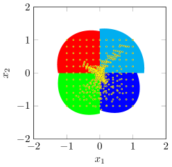
(a) First overapproximation found by (PSD)

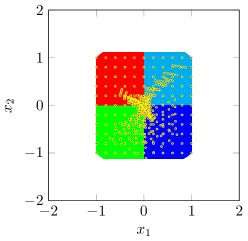
(b) Final overapproximation found by policy iterations

Figure 1: (Discretized) $\mathcal{R}$ in yellow and initial and last overapproximations of $\mathcal{R}$.

Finally, we find after two iterations that for all $k\in\mathbb{N}$, $x_{1,k}^{2}\leq 1,\ x_{2,k}^{2}\leq 1.2443$ and $L(x_{1,k},x_{2,k})\leq 2$.

6.2 A (piecewise) affine example

We now consider the following PWA: $X^{0}=[0,3]\times[0,2]$ and for all $k\in\mathbb{N}$:

$$\begin{array}[]{l}x_{k+1}=\left\{\begin{array}[]{lr}A^{1}x_{k}+b^{1}&\text{ if }T(x_{k})<c\\ A^{2}x_{k}+b^{2}&\text{ if }T(x_{k})\geq c\\ \end{array}\right.\end{array}$$

with

$$\begin{array}[]{c}A^{1}=\begin{pmatrix}0.4197&-0.2859\\ 0.5029&0.1679\\ \end{pmatrix},\quad b^{1}=\begin{pmatrix}2.0000\\ 5.0000\end{pmatrix},\\ A^{2}=\begin{pmatrix}-0.0575&-0.4275\\ -0.3334&-0.2682\\ \end{pmatrix},\quad b^{2}=\begin{pmatrix}-4.0000\\ 4.0000\end{pmatrix}\\ \\ T=\begin{pmatrix}3.0000&8.0000\end{pmatrix}\text{ and }c=-3.0000\end{array}$$

By Prop. 1, $\overline{\mathrm{Sw}}=\mathcal{I}^{2}=\{(1,1),(1,2),(2,1),(2,2)\}$ and $\mathrm{In}=\{2\}$. Using Problem (PSD), we compute the PQL function $L$ characterized by:

$$\begin{array}[]{c}P^{1}=\begin{pmatrix}2.9888&-1.7890\\ -1.7890&8.0295\end{pmatrix},\quad q^{1}=\begin{pmatrix}-14.7283\\ -94.1347\end{pmatrix}\\ \text{and}\\ P^{2}=\begin{pmatrix}2.7192&2.0930\\ 2.0930&6.1110\end{pmatrix},\quad q^{2}=\begin{pmatrix}5.5737\\ -16.4198\end{pmatrix}\\ \end{array}$$

and the invariant found is $\{x\in\mathbb{R}^{2}\mid L(x)\leq 58.1165\}$ and an upper bound over the square Euclidian norm of the state variable is $286.4932$. We run the policy iteration to get finally after 4 iterations the following bound vector:

$$w_{1}=41.8956,\ w_{2}=31.4449,\ w_{3}=58.1165$$

corresponding to the invariant set $w\{x\in\mathbb{R}^{2}\mid x_{i}^{2}\leq w_{i},\ L(x)\leq w_{3}\}$.

We obtain interesting information during policy iterations running. At step $k=0$, when we select the initial policy, the SDP solver returns for all $l=1,2,3$, $F^{\mathcal{R}}_{11,l}(w^{0})=-\infty$ and from Prop. 6 this implies that $\sup_{x\in\mathcal{R}\cap X^{1}\cap{f^{1}}^{-1}(X^{1})}p(A^{1}x+b^{1})$ is not feasible hence $(1,1)\notin\mathrm{Sw}$. At iteration step $k=1$, the SDP solver provides for all $l=1,2,3$, $F^{\mathcal{R}}_{21,l}(w^{1})=-\infty$ and from Prop. 6 this implies that $\sup_{x\in\mathcal{R}\cap X^{1}\cap{f^{2}}^{-1}(X^{2})}p(A^{2}x+b^{2})$ is not feasible hence $(2,1)\notin\mathrm{Sw}$. Finally, $\mathrm{Sw}\subseteq\{(1,2),(2,2)\}$. Recalling that $1\notin\mathrm{In}$, we conclude that the system state variable only stays in $X^{2}$ and thus the system is actually equivalent to a constrained affine system. This information is computed automatically.

7 Conclusion and Future Works

We have developed a method to compute automatically by semi-definite programming precise bounds over the reachable values set of a piecewise affine system. The method combines piecewise quadratic Lyapunov functions to generate a first overapproximation and policy iterations used to reduce the initial overapproximation.

Future works could be to design a repartitioning method in order to improve the feasibility of Problem (PSD). Morevoer, we can think of apply the method to maximize a quadratic form over the reachable values set.

Also, we conjecture that the presented policy iterations algorithm provides the most precise overapproximation considering bounding the square of coordinates variables. To reduce these bounds we have to choose a different set of quadratic functions.

Appendix

In the appendix, we give details about the proofs of the propositions.

Proposition 9

Assume that Problem (PSD) has a feasible solution $(\mathcal{P},\mathcal{W},\mathcal{U},\mathcal{Z},\alpha,\beta)$. Then:

1. The family $\mathcal{P}$ defines a PQL;

2. There exists $(\mathcal{P},\mathcal{W},\mathcal{U},\mathcal{Z},\alpha,\beta)$ satisfiying (16), (17) and (18) if and only if Problem (PSD) is feasible;

3. For all $(i,j)\in\overline{\mathrm{Sw}}$,

   $$\begin{array}[]{ll}&{F^{i}}^{\intercal}\mathbf{M}(\operatorname{Id},0,0)F^{i}\\ \preceq&\mathbf{M}(P^{i},2q^{i},-\alpha)+\mathbf{M}(0,0,\beta)\\ &-{E^{ij}}^{\intercal}\left(\begin{pmatrix}0_{n_{i}}&0_{n_{i},n_{j}}\\ 0_{n_{j},n_{i}}&W^{j}_{p}+W^{j}_{+}\end{pmatrix}+U^{ij}_{p}+U^{ij}_{+}\right)E^{ij}\enspace;\end{array}$$

4. We have $\displaystyle{\sup_{x\in X^{0}}\mbox{$\|x\|$}_{2}^{2}}\leq\beta$;

5. If $(\mathcal{P},\mathcal{W},\mathcal{U},\mathcal{Z},\alpha,\beta)$ is optimal and $\alpha>0$ then $\displaystyle{\sup_{x\in X^{0}}L(x)}=\alpha$.

Proof 8

(1) The first statement follows readily from Corollary ($\star$ ‣ 1).

(2) The "if" part is obvious. Let us focus on the "only if" part and let $(\mathcal{P},\mathcal{W},\mathcal{U},\mathcal{Z},\alpha,\beta)$ satisfiying (16), (17). From Th. 1, $\beta\geq 0$. If $\alpha\geq 0$, the proof is finished. Hence, we suppose that $\alpha<0$ and let us prove that $(\mathcal{P},\mathcal{W},\mathcal{U},\mathcal{Z},0,\beta-\alpha)$ is feasible for Problem (PSD). First $\beta-\alpha\geq 0$ since $\beta\geq 0$ and $\alpha<0$. Second, $\mathbf{M}(P^{i},2q^{i},0)-\mathbf{M}(\operatorname{Id},0,-(\beta-\alpha))-{E^{i}}^{\intercal}\left(W^{i}_{p}+W^{i}_{+}\right)E^{i}=\mathbf{M}(P^{i},2q^{i},-\alpha)-\mathbf{M}(\operatorname{Id},0,-\beta)-{E^{i}}^{\intercal}\left(W^{i}_{p}+W^{i}_{+}\right)E^{i}\succeq 0$ by the fact that $(\mathcal{P},\mathcal{W},\mathcal{U},\mathcal{Z},\alpha,\beta)$ satisfies (16) and thus $(\mathcal{P},\mathcal{W},\mathcal{U},\mathcal{Z},0,\beta-\alpha)$ satisfies (16). Since $\alpha$ and $\beta$ do not appear in (17), $(\mathcal{P},\mathcal{W},\mathcal{U},\mathcal{Z},0,\beta-\alpha)$ satisfies (17). Finally,

$$\begin{array}[]{cl}&-\mathbf{M}(P^{i},2q^{i},0)-{E^{i0}}^{\intercal}\left(Z^{0i}_{p}+Z^{0i}_{+}\right)E^{i0}\\ =&-\mathbf{M}(P^{i},2q^{i},\alpha-\alpha)-{E^{i0}}^{\intercal}\left(Z^{0i}_{p}+Z^{0i}_{+}\right)E^{i0}\\ =&\mathbf{M}(0,0,-\alpha)-\mathbf{M}(P^{i},2q^{i},-\alpha)-{E^{i0}}^{\intercal}\left(Z^{0i}_{p}+Z^{0i}_{+}\right)E^{i0}\end{array}$$

We conclude that $-\mathbf{M}(P^{i},2q^{i},0)-{E^{i0}}^{\intercal}\left(Z^{0i}_{p}+Z^{0i}_{+}\right)E^{i0}\succeq 0$ and thus $(\mathcal{P},\mathcal{W},\mathcal{U},\mathcal{Z},0,\beta-\alpha)$ satisfies (18).

(3) Let $(i,j)\in\overline{\mathrm{Sw}}$. Since $j\in\mathcal{I}$,

$$\mathbf{M}(P^{j},2q^{j},-\alpha)-\mathbf{M}(\operatorname{Id},0,-\beta)-{E^{j}}^{\intercal}\left(W^{j}_{p}+W^{j}_{+}\right)E^{j}\succeq 0$$

and thus

$$\begin{array}[]{r}{F^{i}}^{\intercal}\left(\mathbf{M}(P^{j},2q^{j},-\alpha)-\mathbf{M}(\operatorname{Id},0,-\beta)\right.\\ \left.-{E^{j}}^{\intercal}\left(W^{j}_{p}+W^{j}_{+}\right)E^{j}\right)F^{i}\succeq 0\end{array}$$

and

$$\begin{array}[]{l}{F^{i}}^{\intercal}\mathbf{M}(P^{j},2q^{j},-\alpha)F^{i}-{F^{i}}^{\intercal}{E^{j}}^{\intercal}\left(W^{j}_{p}+W^{j}_{+}\right)E^{j}F^{i}\\ \succeq{F^{i}}^{\intercal}\mathbf{M}(\operatorname{Id},0,-\beta)F^{i}\end{array}$$

Hence:

$$\begin{array}[]{ll}&{F^{i}}^{\intercal}\mathbf{M}(\operatorname{Id},0,-\beta)F^{i}\\ \preceq&-{F^{i}}^{\intercal}{E^{j}}^{\intercal}\left(W^{j}_{p}+W^{j}_{+}\right)E^{j}F^{i}+\mathbf{M}(P^{i},2q^{i},0)\\ &-{E^{ij}}^{\intercal}\left(U^{ij}_{p}+U^{ij}_{+}\right)E^{ij}\end{array}$$

Note that ${F^{i}}^{\intercal}\mathbf{M}(0,0,-\beta)F^{i}=\mathbf{M}(0,0,-\beta)$ and thus:

$$\begin{array}[]{ll}&{F^{i}}^{\intercal}\mathbf{M}(\operatorname{Id},0,0)F^{i}\\ \preceq&-{F^{i}}^{\intercal}{E^{j}}^{\intercal}\left(W^{j}_{p}+W^{j}_{+}\right)E^{j}F^{i}+\mathbf{M}(P^{i},2q^{i},0)\\ &-{E^{ij}}^{\intercal}\left(U^{ij}_{p}+U^{ij}_{+}\right)E^{ij}+\mathbf{M}(0,0,\beta)\end{array}$$

We conclude by the definition of $E^{ij}$.

(4) Since $(\mathcal{P},\mathcal{W},\mathcal{U},\mathcal{Z},\alpha,\beta)$ defines a PQL function, then the result of Th. 1 holds that is $\mathcal{R}\subseteq\{x\in\mathbb{R}^{d}\mid\mbox{$\|x\|$}_{2}^{2}\leq\beta\}$ and since $X^{0}\subseteq\mathcal{R}$, $\sup_{x\in X^{0}}\mbox{$\|x\|$}_{2}^{2}\leq\beta$.

(5) Now assume that $(\mathcal{P},\mathcal{W},\mathcal{U},\mathcal{Z},\alpha,\beta)$ is an optimal solution such that $\alpha>0$ and suppose that $\sup_{x\in X^{0}}L(x)\neq\alpha$. We remark that $\sup_{x\in X^{0}}L(x)=\sup_{i\in\mathrm{In}}\sup_{x\in X^{i}\cap X^{0}}L^{i}(x)$ and from Constraint (18), for all $i\in\mathrm{In}$, $X^{i}\cap X^{0}\subseteq\{x\mid L^{i}(x)\leq\alpha\}$. Hence for all $i\in\mathrm{In}$, $\sup_{x\in X^{i}\cap X^{0}}L^{i}(x)\leq\alpha$ and thus $\sup_{x\in X^{0}}L(x)\leq\alpha$. Let $\epsilon>0$ such that $\gamma=\alpha-\epsilon\geq 0$ and $\sup_{x\in X^{0}}L(x)\leq\gamma$. Let us denote by $\mathbf{N}$ the matrix defined by $\mathbf{N}_{1,1}=1$ and $\mathbf{N}_{l,m}=0$ for all $(l,m)\in\{1,\ldots,d+1\}^{2}\backslash\{(1,1)\}$. We have $-\mathbf{M}(P^{i},2q^{i},-\gamma)-{E^{i0}}^{\intercal}\left(Z^{0i}_{p}+Z^{0i}_{+}\right)E^{i0}=-\mathbf{M}(L^{i})+\gamma N-{E^{i0}}^{\intercal}\left(Z^{0i}_{p}+Z^{0i}_{+}\right)E^{i0}=(\alpha-\epsilon)N-\mathbf{M}(L^{i})-{E^{i0}}^{\intercal}\left(Z^{0i}_{p}+Z^{0i}_{+}\right)E^{i0}$. Let us remark since ${E_{1,1}^{i0}}$ is equal to 1, that ${E^{i0}}^{\intercal}N{E^{i0}}=N$. Thus,

$$\begin{array}[]{ll}&-\mathbf{M}(P^{i},2q^{i},-\gamma)-{E^{i0}}^{\intercal}\left(Z^{0i}_{p}+Z^{0i}_{+}\right)E^{i0}\\ =&-\mathbf{M}(L^{i})+\alpha N-{E^{i0}}^{\intercal}\left(Z^{0i}_{p}+\epsilon N+Z^{0i}_{+}\right)E^{i0}\enspace.\end{array}$$

In a second time,

$$\begin{array}[]{ll}&\mathbf{M}(P^{i},2q^{i},-\gamma)-\mathbf{M}(\operatorname{Id},0,-\beta)-{E^{i}}^{\intercal}\left(W^{i}_{p}+W^{i}_{+}\right)E^{i}\\ =&\mathbf{M}(P^{i},2q^{i},-\alpha)-\mathbf{M}(\operatorname{Id},0,-\beta)-{E^{i}}^{\intercal}\left(W^{i}_{p}+W^{i}_{+}\right)E^{i}\\ &+\epsilon N\enspace.\end{array}$$

From Constraint (16), $\mathbf{M}(P^{i},2q^{i},-\gamma)-\mathbf{M}(\operatorname{Id},0,-\beta)-{E^{i}}^{\intercal}\left(W^{i}_{p}+W^{i}_{+}\right)E^{i}$ is positive semidefinite. We conclude that $(\mathcal{P},\mathcal{W},\mathcal{U},\mathcal{Z}^{\prime},\gamma,\beta)$ with $\mathcal{Z}^{\prime}=\{\left(Z^{i0}_{p}+\epsilon N,Z^{i0}_{+}\right)\in\mathbb{S}_{n_{i0}}^{\geq 0}\times\mathbb{S}_{n_{i0}}^{+},i\in\mathrm{In}\}$ is feasible and $\gamma+\beta=\alpha+\beta-\epsilon$ thus $(\mathcal{P},\mathcal{W},\mathcal{U},\mathcal{Z},\alpha,\beta)$ cannot be optimal.

Proposition 10

The following statements hold:

1. $F(C(\omega))\subseteq C(\omega)\iff F^{\sharp}(\omega)\leq\omega$;

2. $\mathcal{R}\subseteq\inf\{C(\omega)\mid\omega\in\mathbb{R}^{d+1}\text{ s.t. }F^{\sharp}(\omega)\leq\omega\}$;

3. For all $l\in[d+1]$, $F_{ij,l}^{\sharp}(\omega)$ is the optimal value of quadratic program;

4. For all $k\in[d]$, $X_{k}^{0}=\displaystyle{\max\{(\inf_{x\in X^{0}}x_{k})^{2},(\sup_{x\in X^{0}}x_{k})^{2}\}}$ and if $L$ is constructed from an optimal solution $(\mathcal{P},\mathcal{W},\mathcal{U},\mathcal{Z},\alpha,\beta)$ of (PSD) such that $\alpha>0$, then $X_{d+1}^{0}=\alpha$.

Proof 9

(1) $F(C(\omega))\subseteq C(\omega)$ iff for all $k\in[d]$, $\sup_{y\in F(C(\omega))}y_{k}^{2}\leq\omega_{k}$ and $\sup_{y\in F(C(\omega))}L(y)\leq\omega_{d+1}$. Now for all $k\in[d]$:

$$\begin{array}[]{ll}&\sup_{y\in F(C(\omega))}y_{k}^{2}\\ =&\sup\{\sup_{y\in\mathbb{A}(C(\omega))}y_{k}^{2},\sup_{y\in X^{0}}y_{k}^{2}\}\\ =&\sup\{\sup_{(i,j)\in\overline{\mathrm{Sw}}}\displaystyle{\sup_{\begin{subarray}{c}y=A^{i}x+b^{i},\\ x\in C(\omega),x\in X^{ij}\end{subarray}}y_{k}^{2}},\sup_{y\in X^{0}}y_{k}^{2}\}\\ =&F_{k}^{\sharp}(\omega)\end{array}$$

and

$$\begin{array}[]{ll}&\sup_{y\in F(C(\omega))}L(y)\\ =&\sup\{\sup_{y\in\mathbb{A}(C(\omega))}L(y),\sup_{y\in X^{0}}L(y)\}\\ =&\sup\{\sup_{(i,j)\in\overline{\mathrm{Sw}}}\displaystyle{\sup_{\begin{subarray}{c}y=A^{i}x+b^{i},\\ x\in C(\omega),\ x\in X^{ij}\end{subarray}}L^{i}(y)},\sup_{y\in X^{0}}L(y)\}\\ =&F_{d+1}^{\sharp}(\omega)\end{array}$$

(2) From Eq. (19), $\mathcal{R}\subseteq\inf\{C(\omega)\mid\omega\in\mathbb{R}^{d+1},\ F^{\sharp}(C(\omega))\subseteq C(\omega)\}$. We conclude using the first point.

(3) Obvious.

(4) Let $k\in[d]$. Since $X^{0}$ is compact and $x\mapsto x_{k}$ is continuous then there exist $z\in X^{0}$ and $u\in X^{0}$ such that $z_{k}=\inf_{x\in X^{0}}x_{k}$ and $u_{k}=\sup_{x\in X^{0}}x_{k}$. Hence $z_{k}\leq x_{k}\leq u_{k}$ for all $x\in X^{0}$ and thus for all $x\in X^{0}$, $x_{k}^{2}\leq\max(z_{k}^{2},u_{k}^{2})$. Since $z$ and $u$ belong to $X^{0}$, then $X^{0}_{k}=\max(z_{k}^{2},u_{k}^{2})$. We have assumed that $(\mathcal{P},\mathcal{W},\mathcal{U},\mathcal{Z},\alpha,\beta)$ is an optimal solution of Problem (PSD) and $\alpha>0$ then ${X^{0}}^{\dagger}(L)=\alpha$ from Prop. 4.

Proposition 11 (Safe overapproximation)

The following assertions are true:

1. For all $l\in[d+1]$, $F_{l}^{\mathcal{R}}$ is the optimal value of a SDP program;

2. $F^{\sharp}\leq F^{\mathcal{R}}$ .

Proof 10

(1) Obvious.

(2) We have to prove that for all $k\in[d+1]$, for all $\omega\in\mathbb{R}^{d+1}$, $F_{ij,k}^{\sharp}(\omega)\leq F_{ij,k}^{\mathcal{R}}(\omega)$. We do the proof for the case $k=d+1$. The other cases follows the same proof constructions.

Applying the weak duality theorem, we obtain:

$$\begin{array}[]{r}F_{ij,d+1}^{\sharp}(\omega)\leq\displaystyle{\inf_{\lambda\in\mathbb{R}_{+}^{d+1}}\sup_{x\in X^{ij}}L^{j}(f^{i}(x))+\sum_{k=1}^{d}\lambda_{k}(\omega_{k}-x_{k}^{2})}\\ +\lambda_{d+1}(\omega_{d+1}-L^{i}(x))\end{array}$$

Using Lemma 3 and Corollary 1 we get:

$$\begin{array}[]{ccl}&F_{ij,d+1}^{\sharp}(\omega)\\ \leq&\displaystyle{\inf_{\lambda,\eta}}&\eta\\ &\operatorname{s.t.}&\left\{\begin{array}[]{l}\forall\,x\in X^{ij},\\ \displaystyle{\eta-L^{j}(f^{i}(x))-\sum_{k=1}^{d}\lambda_{k}(\omega_{k}-x_{k}^{2})}\\ \displaystyle{-\lambda_{d+1}(\omega_{d+1}-L^{i}(x))-p(f^{i}(x))\geq 0}\\ \\ \lambda\geq 0,\ \eta\in\mathbb{R}\end{array}\right.\\ \leq&\displaystyle{\inf_{\lambda,\eta}}&\eta\\ &\operatorname{s.t.}&\left\{\begin{array}[]{l}\displaystyle{\mathbf{M}\left(\eta-L^{j}(f^{i}(x))-\sum_{k=1}^{d}\lambda_{k}(\omega_{k}-x_{k}^{2})\right.}\\ \displaystyle{\left.-\lambda_{d+1}(\omega_{d+1}-L^{i}(x))\right)}\in\mathbf{C}_{d+1}\left(E^{ij}\right)\\ \\ \lambda\in\mathbb{R}_{+}^{d+1},\ \eta\in\mathbb{R}\end{array}\right.\\ \leq&\displaystyle{\inf_{\lambda,\eta,Y,Z}}&\eta\\ &\operatorname{s.t.}&\left\{\begin{array}[]{l}\displaystyle{\mathbf{M}\left(\eta-L^{j}(f^{i}(x))-\sum_{k=1}^{d}\lambda_{k}(\omega_{k}-x_{k}^{2})\right.}\\ \displaystyle{\left.-\lambda_{d+1}(\omega_{d+1}-L^{i}(x))\right)}-{E^{ij}}^{\intercal}(Y+Z)E^{ij}\\ \succeq 0\\ \\ \lambda\in\mathbb{R}_{+}^{d+1},\ \eta\in\mathbb{R},\ Y\geq 0,\ Z\succeq 0\end{array}\right.\end{array}$$

Now from Eq. (9) and since $A\to\mathbf{M}(A)$ is linear, we have:

$$\begin{array}[]{l}\displaystyle{\mathbf{M}\left(\eta-L^{j}(f^{i}(x))-\sum_{k=1}^{d}\lambda_{k}(\omega_{k}-x_{k}^{2})-\lambda_{d+1}(\omega_{d+1}-L^{i}(x))\right)}\\ \displaystyle{=(\eta-\sum_{k=1}^{d+1}\lambda_{k}\omega_{k})N-{F^{i}}^{\intercal}M_{L}^{j}F^{i}+\sum_{k=1}^{d}\lambda_{k}M_{k}+\lambda_{d+1}M_{L}^{i}}\\ =\displaystyle{(\eta-\sum_{k=1}^{d+1}\lambda_{k}\omega_{k})N-\Phi_{ij,d+1}(\lambda,Y,Z)}+{E^{ij}}^{\intercal}(Y+Z)E^{ij}\end{array}$$

Finally: $\mathbf{M}(\eta-L^{j}(f^{i}(x))-\sum_{k=1}^{d}\lambda_{k}(\omega_{k}-x_{k}^{2})-\lambda_{d+1}(\omega_{d+1}-L^{i}(x)))-{E^{ij}}^{\intercal}(Y+Z)E^{ij}=(\eta-\sum_{k=1}^{d+1}\lambda_{k}\omega_{k})N-\Phi_{ij,d+1}(\lambda,Y,Z)$. Since $F_{ij,l}^{\mathcal{R}}$ is the infimum of $\eta$ over the constraint $(\eta-\sum_{k=1}^{d+1}\lambda_{k}\omega_{k})N-\Phi_{ij,d+1}(\lambda,Y,Z)\succeq 0$, $\lambda\in\mathbb{R}_{+}^{d+1},\ \eta\in\mathbb{R},\ Y\geq 0$ and $Z\succeq 0$, this achieves the proof.

Proposition 12

Let $(i,j)\in\overline{\mathrm{Sw}}$, $l\in[d+1]$, $\lambda\in\mathbb{R}_{+}^{d+1}$. The following statements are true:

1. $F_{ij,l}^{\lambda}$ is affine;

2. $F_{ij,l}^{\lambda}$, $F_{ij,l}^{\mathcal{R}}$ and $F_{l}^{\mathcal{R}}$ are monotone;

3. $F_{ij,l}^{\mathcal{R}}$ and $F_{l}^{\mathcal{R}}$ are upper semi-continuous.

Proof 11

The first assertion is straightforward from Equation (22). The function $w\mapsto F_{ij,l}^{\lambda}(w)$ is monotone from the positivity of $\lambda$ and the two last functions comes are monotone as the supremum of monotone functions. The function $w\mapsto F_{ij,l}^{\mathcal{R}}(w)$ is upper semi-continuous as the infimum of continuous functions and $w\mapsto F_{l}^{\mathcal{R}}(w)$ is upper semi-continuous as the finite supremum of upper semi-continuous functions.

Proposition 13

The vector $\omega^{0}$ satisfies $F^{\mathcal{R}}(\omega^{0})\leq\omega^{0}$.

Proof 12

From Prop. 4, we have for all $k\in[d]$, $X_{k}^{0}\leq\beta=\omega_{k}^{0}$ and $X_{d+1}^{0}=\alpha=\omega_{d+1}^{0}$.

Then it suffices to prove that for all $l\in[d+1]$, for all $(i,j)\in\overline{\mathrm{Sw}}$, $F_{ij,l}^{\mathcal{R}}(\omega^{0})\leq\omega^{0}$. We can show it by proving that for all $l\in[d+1]$, for all $(i,j)\in\overline{\mathrm{Sw}}$, there exist $\lambda\geq 0$, $Y\geq 0$ and $Z\succeq 0$ such that:

$$(\omega_{l}^{0}-\sum_{k=1}^{d+1}\lambda_{k}\omega_{k})N-\Phi_{ij,l}(\lambda,Y,Z)\succeq 0$$

Let us define $\bar{\lambda}$ by $\bar{\lambda}_{d+1}=1$ and $\bar{\lambda}_{k}=0$ for all $k\in[d]$. Let $(i,j)\in\overline{\mathrm{Sw}}$.

Recall that $(\mathcal{P},\mathcal{W},\mathcal{U},\mathcal{Z},\alpha,\beta)$ is an optimal solution of Problem (PSD). Let $l=d+1$, and let us extract $U^{ij}_{p}$ and $U^{ij}_{+}$ from $\mathcal{U}$, then we have:

$$\begin{array}[]{l}(\omega_{d+1}^{0}-\sum_{k=1}^{d+1}\bar{\lambda}_{k}\omega_{k})N-\Phi_{ij,l}(\bar{\lambda},U^{ij}_{p},U^{ij}_{+})\\ =-{F^{i}}^{\intercal}\mathbf{M}_{L}^{j}F^{i}+\mathbf{M}_{L}^{i}-{E^{ij}}^{\intercal}(U^{ij}_{p}+U^{ij}_{+})E^{ij}\end{array}$$

We conclude that $(\omega_{d+1}^{0}-\sum_{k=1}^{d+1}\bar{\lambda}_{k}\omega_{k})N-\Phi_{ij,l}(\bar{\lambda},U^{ij}_{p},U^{ij}_{+})\succeq 0$ since $(\mathcal{P},\mathcal{W},\mathcal{U},\mathcal{Z},\alpha,\beta)$ is an optimal solution of Problem (PSD) and thus satisfies (17). We conclude that $(\omega_{d+1}^{0},\bar{\lambda},U^{ij}_{p},U^{ij}_{+})$ is a feasible solution of the SDP problem (21) and thus $F_{ij,d+1}^{\mathcal{R}}(\omega^{0})\leq\omega_{d+1}^{0}$.

Let $l\in[d]$, $\bar{Y}=\left(\begin{smallmatrix}0_{n_{i}}&0_{n_{i},n_{j}}\\ 0_{n_{j},n_{i}}&W^{j}_{p}\end{smallmatrix}\right)+U^{ij}_{p}$ and $\bar{Z}=\left(\begin{smallmatrix}0_{n_{i}}&0_{n_{i},n_{j}}\\ 0_{n_{j},n_{i}}&W^{j}_{+}\end{smallmatrix}\right)+U^{ij}_{+}$ where $W^{j}_{p}$ and $W^{j}_{+}$ are extracted from $\mathcal{W}$ and $U^{ij}_{p}$ and $U^{ij}_{+}$ are extracted from $\mathcal{U}$. We have:

$$\begin{array}[]{l}(\omega_{l}^{0}-\sum_{k=1}^{d+1}\bar{\lambda}_{k}\omega_{k})N-\Phi_{ij,l}(\bar{\lambda},\bar{Y},\bar{Z})\\ =\mathbf{M}(0,0,\beta-\alpha)-{F^{i}}^{\intercal}\mathbf{M}_{l}F^{i}+\mathbf{M}_{L}^{i}-{E^{ij}}^{\intercal}(\bar{Y}+\bar{Z})E^{ij}\end{array}$$

Now, remark that $\mathbf{M}_{l}\preceq\mathbf{M}(\operatorname{Id},0,0)$ and thus $-{F^{i}}^{\intercal}\mathbf{M}_{l}F^{i}+\mathbf{M}(P^{i},2q^{i},-\alpha)-{E^{ij}}^{\intercal}(\bar{Y}+\bar{Z})E^{ij}+\mathbf{M}(0,0,\beta)\preceq-{F^{i}}^{\intercal}\mathbf{M}(\operatorname{Id},0,0)F^{i}+\mathbf{M}(P^{i},2q^{i},-\alpha)-{E^{ij}}^{\intercal}(\bar{Y}+\bar{Z})E^{ij}+\mathbf{M}(0,0,\beta)$. The right-hand-side sum of matrices is positive semi-definite from the second assertion of Prop. 4. We conclude that $(\omega_{l}^{0}(p),\bar{\lambda},\bar{Y},\bar{Z})$ is a feasible solution of the SDP problem (21) and thus $F_{ij,l}^{\mathcal{R}}(\omega^{0})\leq\omega_{l}^{0}$.

References

- [Adj14] A. Adjé. Policy iteration in finite templates domain. In Numerical Software Verification (NSV 2014), 2014.
- [AG15] A. Adjé and P.-L. Garoche. Automatic synthesis of piecewise linear quadratic invariants for programs. In Verification, Model Checking, and Abstract Interpretation - 16th International Conference, VMCAI 2015, Mumbai, India, January 12-14, 2015. Proceedings, pages 99–116, 2015.
- [AGG12] A. Adjé, S. Gaubert, and E. Goubault. Coupling policy iteration with semi-definite relaxation to compute accurate numerical invariants in static analysis. Logical Methods in Computer Science, 8(1), 2012.
- [All09] X. Allamigeon. Static analysis of memory manipulations by abstract interpretation — Algorithmics of tropical polyhedra, and application to abstract interpretation. PhD thesis, École Polytechnique, Palaiseau, France, November 2009.
- [BD09] S. Bundfuss and M. Dür. An adaptive linear approximation algorithm for copositive programs. SIAM J. on Optimization, 20(1):30–53, March 2009.
- [BSU12] I. M. Bomze, W. Schachinger, and G. Uchida. Think co(mpletely)positive ! matrix properties, examples and a clustered bibliography on copositive optimization. Journal of Global Optimization, 52(3):423–445, 2012.
- [CGG+05] A. Costan, S. Gaubert, E. Goubault, M. Martel, and S. Putot. A policy iteration algorithm for computing fixed points in static analysis of programs. In Computer aided verification, pages 462–475. Springer, 2005.
- [Dia62] P. H. Diananda. On non-negative forms in real variables some or all of which are non-negative. Mathematical Proceedings of the Cambridge Philosophical Society, 58:17–25, 1 1962.
- [GGTZ07] S. Gaubert, E. Goubault, A. Taly, and S. Zennou. Static analysis by policy iteration on relational domains. In Programming Languages and Systems, pages 237–252. Springer, 2007.
- [GSA+12] T. Gawlitza, H. Seidl, A. Adjé, S. Gaubert, and E. Goubault. Abstract interpretation meets convex optimization. J. Symb. Comput., 47(12):1416–1446, 2012.
- [HK66] A. J. Hoffman and R. M. Karp. On nonterminating stochastic games. Management Science, 12(5):359–370, 1966.
- [How60] R. A. Howard. Dynamic Programming and Markov Processes. MIT Press, Cambridge, MA, 1960.
- [Joh03] M. Johansson. On modeling, analysis and design of piecewise linear control systems. In Circuits and Systems, 2003. ISCAS ’03. Proceedings of the 2003 International Symposium on, volume 3, pages III–646–III–649 vol.3, May 2003.
- [Mas12] D. Massé. Proving termination by policy iteration. Electronic Notes in Theoretical Computer Science, 287(0):77 – 88, 2012. Proceedings of the Fourth International Workshop on Numerical and Symbolic Abstract Domains, NSAD 2012.
- [MFTM00] D. Mignone, G. Ferrari-Trecate, and M. Morari. Stability and stabilization of piecewise affine and hybrid systems: an lmi approach. In Decision and Control, 2000. Proceedings of the 39th IEEE Conference on, volume 1, pages 504–509 vol.1, 2000.
- [MJ81] D.H. Martin and D.H. Jacobson. Copositive matrices and definiteness of quadratic forms subject to homogeneous linear inequality constraints. Linear Algebra and its Applications, 35(0):227 – 258, 1981.
- [MM62] J. E. Maxfield and H. Minc. On the matrix equation X′X = A. Proceedings of the Edinburgh Mathematical Society (Series 2), 13:125–129, 12 1962.
- [Mot51] T. S. Motzkin. Two consequences of the transposition theorem on linear inequalities. Econometrica, 19(2):184–185, 1951.
- [RJGF12] P. Roux, R. Jobredeaux, P.-L. Garoche, and E. Feron. A generic ellipsoid abstract domain for linear time invariant systems. In Hybrid Systems: Computation and Control (part of CPS Week 2012), HSCC’12, Beijing, China, April 17-19, 2012, pages 105–114, 2012.
- [SJVG11] P. Sotin, B. Jeannet, F. Védrine, and E. Goubault. Policy iteration within logico-numerical abstract domains. In Automated Technology for Verification and Analysis, pages 290–305. Springer, 2011.
- [SS13] P. Schrammel and P. Subotic. Logico-numerical max-strategy iteration. In Roberto Giacobazzi, Josh Berdine, and Isabella Mastroeni, editors, Verification, Model Checking, and Abstract Interpretation, volume 7737 of Lecture Notes in Computer Science, pages 414–433. Springer Berlin Heidelberg, 2013.
- [Tar55] A. Tarski. A lattice-theoretical fixpoint theorem and its applications. Pacific J. Math., 5(2):285–309, 1955.
- [Vav90] S. A. Vavasis. Quadratic programming is in NP. Information Processing Letters, 36(2):73 – 77, 1990.