NCTS-TH/1501

Dilaton,
Screening of the Cosmological Constant and IR-Driven Inflation

Chong-Sun Chu${\,}^{a,b}$ and Yoji Koyama${\,}^{a}$

${}^{a}\,$Physics Division, National Center for Theoretical Sciences,
National Tsing-Hua University, Hsinchu, 30013, Taiwan
${}^{b}\,$Department of Physics, National Tsing-Hua University, Hsinchu 30013, Taiwan

It is known that infrared (IR) quantum fluctuations in de Sitter space could break the de Sitter symmetry and generate time dependent observable effects. In this paper, we consider a dilaton-gravity theory. We find that gravitational IR effects lead to a time dependent shift on the vev of the dilaton and results in a screening (temporal) of the cosmological constant/Hubble parameter. In the Einstein frame, the effect is exponentiated and can give rises to a much more notable amount of screening. Taking the dilaton as inflaton, we obtain an inflationary expansion of the slow roll kind. This inflation is driven by the IR quantum effects of de Sitter gravity and does not rely on the use of a slow roll potential. As a result, our model is free from the eta problem which baffle the standard slow roll inflation models.

1 Introduction

It is widely believed that the universe has underwent a period of accelerated expansion in the early cosmology. Such a period of inflation not only solves the flatness and horizon problems of the standard cosmology, but also, with the introduction of an inflaton scalar field and an almost flat potential, predicts a nearly scale invariant density perturbation. This picture is in excellent agreement with observational results of the cosmic microwave background (CMB) and the large scale structure of the universe. However this simple picture is not without problem as it has proven extremely difficult to bring together the inflationary paradigm with fundamental particle physics. For example, Planck mass suppressed corrections to the inflaton potential generally lead to large corrections to the inflaton mass, resulting in a large slow roll parameter $\eta$ which renders prolonged slow roll inflation impossible. One may resort to symmetries such as supersymmetry, global symmetries or higher dimensional gauge symmetries to protect the potential. However supersymmetry only alleviates the problem as supersymmetry must be spontaneously broken at the Hubble scale during inflation; while in the latter approaches approach, a precise control of the Planck suppressed operators breaking the symmetry is needed, and hence the necessity of a full treatment in a theory quantum gravity, e.g. string theory. Interesting effective theories with novel physical effects have been inspired and constructed in string theory, for example, D-brane inflation [2], DBI inflation [4] and axion monodromy inflation [6]. Nevertheless, the construction of inflation model with controllable quantum corrections remains a significant obstacle.

One of the motivation of this work is the desire to come up with a new mechanism to drive inflation that does not employ a slow roll potential.

Dark energy presents another deep mystery of the universe. A common feature shared by both inflation and dark energy is that both involve a cosmological expansion described by a de Sitter metric. The current cosmological constant is of the order of $10^{-120}M_{P}^{2}$. The deep mystery of the cosmological constant problem [8] is to understand why is there such a huge hierarchy of scales between the current cosmological constant and the Planck scale or some high energy scale. It is natural to suspect that a good understanding of the quantum properties of de Sitter space would be necessary in order to tackle this problem properly. It has been conjectured some time ago that IR quantum effects in de Sitter space could lead to a kind of screening to the cosmological constant [13, 16] and provide a resolution to the cosmological constant problem. Explicit de Sitter breaking IR effect has been identified [18, 19, 20, 21] and demonstrated to lead to a weakening effect (over time) on the cosmological constant [22]. Similar effects on the couplings of the matter sector have also been found [23, 24]. However the effects of the screening as obtained from the perturbation theory are usually small. This is still the case even if one may re-sum the perturbation result and extend it’s regime of validity. For other studies of IR effects of quantum theory in de Sitter space, see for example [25]-[38].

Another motivation of this work is to identify new concrete mechanism for the screening of the cosmological constant in which the screening can be sizable, and yet the theory remains in a reliable regime.

In this paper, we consider a theory consisting of a dilaton field coupled to gravity. This is part of the low energy effective theory of the NS-NS sector in any string model building. The dilaton has a potential but its detailed form is not important to us. We will only need to assume that the theory admits a minimum where the dilaton is taking a vacuum expectation value (vev) $\phi=v,\quad v\in{\bf R}$, and the corresponding potential energy is positive; thereby giving rises to a de Sitter metric. As is well known for de Sitter space, the quantum fluctuations of a massless minimal coupled scalar field grows linearly with time and breaks the de Sitter symmetry [18]. In fact the propagator of a massless minimal coupled scalar is IR divergent (see (2.41) below) and breaks the de Sitter symmetry explicitly [19, 20, 21]. The time dependent origin of the IR divergence is simple and can be traced back to the exponential increase in the number of degrees of freedom outside the Hubble horizon. The dilaton in our theory is massive and is not minimally coupled. However part of the graviton excitation modes are massless minimally coupled and so the time dependent IR effects inherent in them could generate time dependent effects on other physical quantities of theory. In this paper, we identify such an effect on the vev of the dilaton field. We find that the IR effects of the gravitational loops (one loop order) induce a time dependence in the vev

$$v\to v_{\rm eff}:=v+\delta v(t),\quad\mbox{where $\delta v\propto(H_{0}t)^{2}$}.$$ (1.1)

Here $H_{0}$ is the Hubble parameter.

As the modification grows quadratically with time, perturbation theory will eventually break down and this imposes a serve limit on the size of this effect. In particle theory, it is possible to re-sum the leading order time dependent corrections by employing the dynamical renormalization group (DRG) equation [39] and obtain a result which has a much bigger regime of validity. The resummation of the IR divergences and the understanding of the associated late time secular evolution in quantized gravity is, however, a much more difficult open problem. For the case of a massive scalar field in de Sitter space with non-derivative self-interaction, the problem is simpler. Over the years various approaches have been proposed and considered, for example, the semiclassical stochastic methods [40], DRG [41, 42], Schwinger-Dyson equation [43]. Although qualitatively similar results are obtained, e.g. on the generation of dynamical mass [44], these different approaches do not report exactly the same results on the non-perturbative resummation. This is presumably due to different aspect of physics were being emphasized and hence slightly different approximations and assumptions have been made correspondingly. For example, stochastic inflation relies on the assumption of a Gaussian probability distribution for the background quantities. In the approaches of Schwinger-Dyson or DRG, it is inevitable to truncate the full set of Feynman diagrams or renormalization group (RG) equations to a manageable subset, leading to disregarding set of diagrams or RG flows that may not be subleading at all in the IR [45]. In general model with derivative interaction, including the case of gravity, the problem is much more difficult and much less is known: the Schwinger-Dyson equation is far too complicated; and it is not know how to generalize the stochastic approach in this case (see however [46] for some suggestions). Comparatively, the DRG approach is relatively simpler. Therefore in this paper we will adopt the DRG approach to resum the leading IR divergences. We believe the time dependent behaviour we found are qualitatively correct although the precise details may be different. We do warn the reader that we are not claiming that we have solved the important open problem of determining the secular IR effects of quantized gravity.

Due to the time dependence (1.1) of the vev, the Hubble parameter of the theory becomes time dependent and decreases slowly with time. That it is slowly changing can be confirmed from the small values of the associated slow roll parameters. Since these slow roll parameters measure the back reaction of the quantum effects on the classical de Sitter background, their smallness means we can trust the result of the perturbative computation.

The above analysis are performed in the string frame. To examine the physical significance of the time dependence of the vev, we need to go to the Einstein frame. As a result of the change of frame, the time dependent effect gets magnified exponentially. We have thus obtained a mechanism of screening of the cosmological constant where a significant amount of screening can be achieved within a calculable and reliable framework. The screening is due to the de Sitter symmetry breaking IR effect of the graviton loops. The behavior of the Hubble parameter in the Einstein frame is one of the slow roll inflation. However there is no almost flat potential and inflation is not achieved by the slow rolling of the inflaton field. Therefore we have obtained a model of inflation where the inflationary expansion is driven by the de Sitter symmetry breaking gravitational IR effect. In particular, it is important to note that since our mechanism does not rely on the existence of a slow roll potential, our model is free from the eta problem which baffles the standard slow roll inflation models.

The plan of the paper is as follows. In section 2, we introduce our model. The classical solution of the theory is discussed in section 2.1. In section 2.2, we set up the perturbation theory. In section 2.3, we use the in-in formalism to compute the time dependent IR corrections on the vev at 1 loop order. In section 2.4, we compute the slow roll parameters and demonstrated that they are small. We then go to the Einstein frame in section 3. In section 3.1, by demanding that the Planck mass is time independent, we fix the choice of frame and obtain the Einstein frame Hubble parameter. This is shown to be of slow roll type in section 3.2. In section 3.3, we look at some different choices of parameters of the model and demonstrate that the de Sitter symmetry breaking IR effect could provide sufficient screening during inflation. This offer an explanation of why the Hubble parameter during inflation is so much smaller compared to the Planck scale (approximately $10^{-4}$ of it).

2 Perturbative Analysis in the String Frame

We consider Einstein gravity coupled non-minimally to a scalar field $\phi$ described by the action

$$S=\int\sqrt{-{g}}d^{4}x\left[\frac{M^{2}}{2}e^{-2\phi/\eta}{R}-\frac{1}{2}{g}^{\mu\nu}\partial_{\mu}\phi\partial_{\nu}\phi-V(\phi)\right].\\$$ (2.1)

Here $M$ is a mass parameter that set the fundamental scale of the theory. The coupling of the scalar field $\phi$ to gravity is described by an exponential coupling $e^{-2\phi/\eta}$ whose strength is controlled by the the dimensionful coupling constant $\eta$. The limit $\eta\to\infty$ corresponds to a minimally coupled theory, where the effects we computed in this paper, e.g. (2.68), will go away. We have also included a potential term $V$. We will not need to assume any particular details for it except for the assumption that a vev $v>0$ is developed for a stable vacuum.

The action (2.1) without the potential term is simply the Jordan-Brans-Dicke theory [47, 48], in which case the scalar field is simply a phenomenological possibility. In string theory, $\phi$ arises necessary as the dilaton of the closed string sector. The general form of the string frame, gravi-dilaton low energy effective action, to the lowest order in the $\alpha^{\prime}$, has been argued to take the form [49],

$$S=\frac{M^{2}}{2}\int\sqrt{-{g}}d^{4}x\left[B_{g}(\phi)R-\frac{B_{\phi}(\phi)}{2}(\partial\phi)^{2}+\frac{2}{M^{2}}V(\phi)\right].$$ (2.2)

Here the “form factors” $B_{g}(\phi),B_{\phi}(\phi)$ include the dilaton-dependent loop corrections and other effects of the background flux, compactification, branes configuration etc; and $V(\phi)$ is an effective dilaton potential. The action (2.1) can be considered as a special case of (2.2). In this paper we will take the phenomenological approach without worrying the embedding of our action in string theory. Our model is specified by the value of the parameter $\eta$ and the potential $V$. However our results do not depend on the specific knowledge of $V$ .

2.1 The de-Sitter vacuum

We begin by analyzing the classical dynamics of the theory (2.1). The equations of motion are:

$$\square\phi-V^{\prime}(\phi)-\frac{M^{2}}{\eta}e^{-2\phi/\eta}{R}=0,$$ (2.3)

$$R_{\mu\nu}-\frac{1}{2}{R}{g}_{\mu\nu}=\frac{1}{M^{2}}{\bar{T}}_{\mu\nu}.$$ (2.4)

Here $\square\phi=\frac{1}{\sqrt{-{g}}}\partial_{\mu}(\sqrt{-{g}}{g}^{\mu\nu}\partial_{\nu}\phi)$ and

$${\bar{T}}_{\mu\nu}=e^{2\phi/\eta}\left[\partial_{\mu}\phi\partial_{\nu}\phi-g_{\mu\nu}(\frac{1}{2}(\partial\phi)^{2}+V(\phi))+M^{2}(D_{\mu}D_{\nu}-g_{\mu\nu}D^{2})e^{-2\phi/\eta}\right],$$ (2.5)

and $D_{\mu}$ is the covariant derivative. The scalar equation can be simplified by substituting the trace of the Einstein equation (2.4)

$${R}=\frac{4}{M^{2}}e^{2\phi/\eta}V(\phi)+\frac{e^{2\phi/\eta}}{M^{2}}\left(1+12\frac{M^{2}}{\eta^{2}}e^{-2\phi/\eta}\right)\partial_{\mu}\phi\partial^{\mu}\phi-\frac{6}{\eta}\square\phi$$ (2.6)

into (2.3) and gets

$$\square\phi-\left(1+6\frac{M^{2}}{\eta^{2}}e^{-2\phi/\eta}\right)^{-1}\left(V^{\prime}(\phi)+\frac{4}{\eta}V(\phi)+\frac{1}{\eta}(1+12\frac{M^{2}}{\eta^{2}}e^{-2\phi/\eta})\partial_{\mu}\phi\partial^{\mu}\phi\right)=0.\quad$$ (2.7)

A solution is given by the de Sitter background:

$$\phi=v\ (\text{const.}),\quad\mbox{such that}\quad V^{\prime}(v)+\frac{4}{\eta}V(v)=0,$$ (2.8)

$$R^{(0)}=\frac{4}{M^{2}}e^{2v/\eta}V(v).$$ (2.9)

We note that the field equation (2.8) for a constant scalar $\phi$ configuration is modified from the usual one by the second term due to its non-minimal coupling to gravity. To get a de-Sitter background, we assume that

$$V(v)>0.$$ (2.10)

Let us also investigate the local stability of the de Sitter solution against small variations. Consider

$$\phi = v+\delta\phi,$$ (2.11)

$${g}_{\mu\nu} = {g}^{\rm dS}_{\mu\nu}+\delta{g}_{\mu\nu}\rightarrow{R}=R^{(0)}+\delta{R}.$$ (2.12)

At ${\cal O}(\delta\phi,\delta{R})$, the scalar field equation becomes

$$\square\delta\phi+(-V^{\prime\prime}(v)+\frac{2M^{2}}{\eta^{2}}e^{-2v/\eta}R^{(0)})\delta\phi-\frac{M^{2}}{\eta}e^{-2v/\eta}\delta{R}=0.$$ (2.13)

On the other hand, $\delta R$ satisfies

$$\delta{R}=\frac{2}{\eta}R^{(0)}\delta\phi+\frac{4}{M^{2}}e^{2v/\eta}V^{\prime}(v)\delta\phi-\frac{6}{\eta}\square\delta\phi.$$ (2.14)

Put $\delta{R}$ into (2.13) we obtain

$$\square\delta\phi-\left(1+\frac{6M^{2}}{\eta^{2}}e^{-2v/\eta}\right)^{-1}\left(V^{\prime\prime}(v)+\frac{4}{\eta}V^{\prime}(v)\right)\delta\phi=0$$ (2.15)

The solution $\phi=v$ is stable for

$$V^{\prime\prime}(v)+\frac{4}{\eta}V^{\prime}(v)>0.$$ (2.16)

The conditions (2.10), (2.8), (2.16) are all that we will assume for the potential $V(\phi)$. This can be easily satisfied. For example any potential that behaves near $\phi=v$ as

$$V(\phi)=V_{0}+\rho(\phi-v)+\frac{\sigma^{2}}{2}(\phi-v)^{2}$$ (2.17)

with

$$V_{0}:=V(v)>0,$$ (2.18)

$$\rho:=V^{\prime}(v)=-\frac{4V_{0}}{\eta},$$ (2.19)

and

$$\sigma^{2}:=V^{\prime\prime}(v)>\frac{16V_{0}}{\eta^{2}}$$ (2.20)

are all right.

2.2 Scalar and graviton propagators

Our central interest is to calculate the graviton one-loop corrections to the vev of the dilaton scalar field in the de Sitter space. We consider the Poincaré coordinate

$$ds^{2}=-dt^{2}+e^{2H_{0}t}d{\bf x}^{2}=a_{0}(\tau)^{2}(-d\tau^{2}+d{\bf x}^{2}),$$ (2.21)

where the Hubble constant is given by the Friedmann equation

$$H_{0}^{2}=\frac{1}{3M^{2}}e^{2v/\eta}V(v),$$ (2.22)

and $\tau$ is the conformal time

$$\tau=-\frac{1}{H_{0}}e^{-H_{0}t}.$$ (2.23)

The scale factor is

$$a_{0}(\tau)=-\frac{1}{H_{0}\tau}.$$ (2.24)

In this paper we will use $H_{0}$ and $H$ to denote the string frame Hubble constant at tree level and at 1-loop, and $H_{E0}$ and $H_{E}$ to denote the Einstein frame Hubble constant at tree level and at 1-loop.

To obtain the perturbative action, we expand $\phi$ around its classical value,

$$\phi=v+{\tilde{\phi}}.$$ (2.25)

In order to construct the scalar and graviton propagators, we begin with the quadratic action in the perturbations:

$$S^{(2)} = \int d^{4}x\left[\frac{1}{\kappa^{2}}\Big{(}(\sqrt{-{g}}{R})^{(2)}-6(\sqrt{-{g}})^{(2)}H_{0}^{2}\Big{)}+\Big{(}\frac{2}{\kappa^{2}\eta}(\sqrt{-{g}}{R})^{(1)}-(\sqrt{-{g}})^{(1)}\rho\Big{)}{\tilde{\phi}}\right.$$ (2.26)

$$\qquad\qquad\left.-\frac{1}{2}a_{0}^{2}\eta^{\mu\nu}\partial_{\mu}{\tilde{\phi}}\partial_{\nu}{\tilde{\phi}}+\frac{1}{2}a_{0}^{4}\left(\frac{48}{\kappa^{2}\eta^{2}}H_{0}^{2}+\sigma^{2}\right){\tilde{\phi}}^{2}\right].$$

We shall adopt the same parametrization of the graviton perturbations as [23, 24],

$${g}_{\mu\nu}=\Omega^{2}(x){{\tilde{g}}}_{\mu\nu},\quad\mathop{\rm det}\nolimits{{\tilde{g}}}_{\mu\nu}=-1$$

$$\Omega(x)=a_{0}(\tau)e^{\kappa\omega(x)},\quad{{\tilde{g}}}_{\mu\nu}=\left(e^{\kappa h}\right)_{\mu\nu},\quad\kappa^{2}=\frac{M^{2}}{2}e^{-2\frac{v}{\eta}},$$ (2.27)

where $\omega$ is the perturbation of the conformal mode, $h$ is the traceless tensor perturbation. Indices on $h_{\mu\nu}$ are raised and lowered with the Lorentz metric $\eta_{\mu\nu}$ and $\eta^{\mu\nu}h_{\mu\nu}=0$. Expanding the graviton perturbations, we obtain

$$S^{(2)} = \int d^{4}x\;a_{0}^{2}\left[-\frac{1}{4}\partial_{\mu}h_{\rho\sigma}\partial^{\mu}h^{\rho\sigma}+\frac{1}{2}\partial_{\mu}h^{\rho\nu}\partial_{\nu}h^{\mu}_{\ \rho}-\frac{1}{2}\eta^{\mu\nu}\partial_{\mu}{\tilde{\phi}}\partial_{\nu}{\tilde{\phi}}\right.$$ (2.28)

$$\qquad\qquad+6\partial_{\mu}\omega\partial^{\mu}\omega-\frac{24}{\tau^{2}}\omega^{2}-2\partial_{\mu}h^{\mu\nu}\partial_{\nu}\omega-\frac{8}{\tau}\omega\partial_{\mu}h^{\mu 0}+\frac{24}{\tau^{2}}h^{00}\omega$$

$$\qquad\qquad+\frac{2}{\kappa\eta}\partial_{\nu}{\tilde{\phi}}\partial_{\mu}h^{\mu\nu}+\frac{8}{\tau\kappa\eta}{\tilde{\phi}}\partial_{\mu}h^{\mu 0}-\frac{24}{\tau^{2}\kappa\eta}{\tilde{\phi}}h^{00}-\frac{12}{\kappa\eta}\partial_{\mu}{\tilde{\phi}}\partial^{\mu}\omega$$

$$\qquad\qquad\left.-\left(\frac{48}{\tau^{2}\kappa\eta}+\frac{4\rho\kappa}{H_{0}^{2}\tau^{2}}\right)\omega{\tilde{\phi}}+\frac{1}{2}\left(\frac{48}{\tau^{2}\kappa^{2}\eta^{2}}-\frac{\sigma^{2}}{H_{0}^{2}\tau^{2}}\right){\tilde{\phi}}^{2}\right].$$

There are the mixing terms among $h_{\mu\nu}$, $\omega$ and ${\tilde{\phi}}$. To obtain canonically normalized fields, let us perform field redefinitions [51, 52] as follows,

$${\hat{h}}_{\mu\nu}=h_{\mu\nu},\qquad{\omega}={\hat{\omega}}+\frac{\zeta}{\kappa\eta}{\hat{\phi}},\qquad{\tilde{\phi}}=\zeta{\hat{\phi}},$$ (2.29)

where $\zeta$ is given by

$$\zeta=\left(1+\frac{12}{\kappa^{2}\eta^{2}}\right)^{-1/2}=\left(1+6\frac{M^{2}}{\eta^{2}}e^{-2v/\eta}\right)^{-1/2}$$ (2.30)

and we have used the classical equation of motion (2.8), which reads

$$\rho+\frac{24}{\kappa^{2}\eta}H_{0}^{2}=0.$$ (2.31)

when expressed in terms of $\rho$, $\kappa$ and $H_{0}$. In terms of the new fields, we have

$$S^{(2)} = \int d^{4}xa_{0}^{2}\left[-\frac{1}{4}\partial_{\mu}h_{\rho\sigma}\partial^{\mu}h^{\rho\sigma}+\frac{1}{2}\partial_{\mu}h^{\rho\nu}\partial_{\nu}h^{\mu}_{\ \rho}+6\partial_{\mu}{\hat{\omega}}\partial^{\mu}{\hat{\omega}}-\frac{24}{\tau^{2}}{\hat{\omega}}^{2}\right.$$ (2.32)

$$\qquad\left.-2\partial_{\mu}h^{\mu\nu}\partial_{\nu}{\hat{\omega}}-\frac{8}{\tau}{\hat{\omega}}\partial_{\mu}h^{\mu 0}+\frac{24}{\tau^{2}}h^{00}{\hat{\omega}}-\frac{1}{2}\eta^{\mu\nu}\partial_{\mu}{\hat{\phi}}\partial_{\nu}{\hat{\phi}}-\frac{1}{2}a_{0}^{2}m^{2}_{\hat{\phi}}{\hat{\phi}}^{2}\right],$$

where the mass of ${\hat{\phi}}$ is

$$m^{2}_{\hat{\phi}}=\zeta^{2}\left(\sigma^{2}+\frac{4\rho}{\eta}\right).$$ (2.33)

The quadratic action $S^{(2)}$ is now written in the standard canonical form for graviton perturbations and a massive scalar field with mass $m_{\hat{\phi}}$. It is known that the propagator for massive scalar field in de Sitter space is given by the hypergeometric function [19]

$$\langle{\hat{\phi}}(x){\hat{\phi}}(x^{\prime})\rangle=\frac{H_{0}^{2}}{(4\pi)^{2}}\Gamma\left(\frac{3}{2}+\nu\right)\Gamma\left(\frac{3}{2}-\nu\right){}_{2}F_{1}\left(\frac{3}{2}+\nu,\frac{3}{2}-\nu;2;1-\frac{y}{4}\right)$$ (2.34)

with $\nu=\sqrt{\frac{9}{4}-\frac{m_{\hat{\phi}}^{2}}{H_{0}^{2}}}$, where the de Sitter invariant length $y$ is defined by

$$y\equiv\frac{-(\tau-\tau^{\prime})^{2}+({\vec{x}}-{\vec{x}}^{\prime})^{2}}{\tau\tau^{\prime}}.$$ (2.35)

For the graviton propagator, let us introduce the following form of the gauge fixing term [53]

$${\cal L}_{\rm GF}=-\frac{1}{2}a_{0}^{2}\eta^{\mu\nu}F_{\mu}F_{\nu},\quad F_{\mu}=\partial_{\rho}h_{\mu}^{\,\rho}-2\partial_{\mu}{\hat{\omega}}-\frac{2}{\tau}h_{\mu}^{\,0}-\frac{4}{\tau}\delta^{0}_{\mu}{\hat{\omega}}.$$ (2.36)

The quadratic terms of the graviton perturbations in the gauge-fixed action are

$$S^{(2)}_{\rm gr} = \int d^{4}x\;a_{0}^{2}\left[\ \frac{1}{2}\eta^{\mu\nu}\partial_{\mu}X\partial_{\nu}X-\frac{1}{4}\eta^{\mu\nu}\partial_{\mu}{\bar{h}}^{i}_{\ j}\partial_{\nu}{\bar{h}}^{j}_{\ i}+\frac{1}{2}\eta^{\mu\nu}\partial_{\mu}h^{0i}\partial_{\nu}h^{0i}\right.$$ (2.37)

$$\qquad\qquad\qquad\left.+a_{0}^{2}H_{0}^{2}h^{0i}h^{0i}-\frac{1}{2}\eta^{\mu\nu}\partial_{\mu}Y\partial_{\nu}Y-a_{0}^{2}H_{0}^{2}Y^{2}\right],$$

where ${\bar{h}}^{i}_{\ j}$, $X$ and $Y$ are defined by

$${\bar{h}}^{i}_{\ j}\equiv h^{i}_{\ j}-\frac{1}{3}h^{k}_{\ k}\delta^{i}_{\ j}=h^{i}_{\ j}-\frac{1}{3}h^{00}\delta^{i}_{\ j},\quad{\bar{h}}^{i}_{\ i}=0,$$ (2.38)

$$X\equiv 2\sqrt{3}{\hat{\omega}}-\frac{1}{\sqrt{3}}h^{00},\hskip 10.00002ptY\equiv h^{00}-2{\hat{\omega}}.$$ (2.39)

Note that the fields ${\bar{h}}^{i}_{\ j}$ and $X$ satisfy the same equation of motion as the massless minimally coupled scalar field; while the fields $h^{0i}$ and $Y$ satisfy the same equation of motion as the massless conformally coupled scalar field. As a result, their propagators are given by

$$\begin{split}\langle{\bar{h}}^{i}_{\ j}(x){\bar{h}}^{k}_{\ l}(x^{\prime})\rangle&=\left(\delta^{ik}\delta_{jl}+\delta^{i}_{\ l}\delta_{j}^{\ k}-\frac{2}{3}\delta^{i}_{\ j}\delta^{k}_{\ l}\right)\langle\varphi(x)\varphi(x^{\prime})\rangle,\\ \langle X(x)X(x^{\prime})\rangle&=-\langle\varphi(x)\varphi(x^{\prime})\rangle,\end{split}$$ (2.40)

where $\varphi$ denotes a massless minimally coupled scalar field,

$$\langle\varphi(x)\varphi(x^{\prime})\rangle=\frac{H_{0}^{2}}{4\pi^{2}}\left(\frac{1}{y}-\frac{1}{2}\ln y+\frac{1}{2}\ln(a_{0}(\tau)a_{0}(\tau^{\prime}))+1-\gamma\right);$$ (2.41)

and

$$\begin{split}\langle h^{0i}(x)h^{0j}(x^{\prime})\rangle&=-\delta^{ij}\frac{H_{0}^{2}}{4\pi^{2}}\frac{1}{y},\quad\langle Y(x)Y(x^{\prime})\rangle=\frac{H_{0}^{2}}{4\pi^{2}}\frac{1}{y}.\end{split}$$ (2.42)

In appendix B, we make comments on the IR properties of the two-point functions of massless minimally coupled scalar fields in de Sitter and flat FRW universe.

We will be computing the quantum shift of the vev of the scalar field by looking at its 1-loop tadpole with various modes running in the loop. It is well known that the de Sitter breaking IR logarithm are generated by massless minimally coupled scalar field, but not by conformally coupled fields, therefore we can neglect the propagation of the (massive) scalar field $\phi$ and the conformally coupled fields $Y$ and $h^{0i}$; and concentrate on the propagation of the modes ${\bar{h}}_{ij}$ and $X$. In this approximation [23, 24],

$$h^{00}\simeq 2{\hat{\omega}}\simeq\frac{\sqrt{3}}{2}X.$$ (2.43)

and we get the following three propagators.

$$\begin{split}\langle{h}^{i}_{\ j}(x){h}^{k}_{\ l}(x^{\prime})\rangle&\simeq(\delta^{ik}\delta_{jl}+\delta^{i}_{\ l}\delta_{j}^{\ k}-\frac{3}{4}\delta^{i}_{\ j}\delta^{k}_{\ l})\langle\varphi(x)\varphi(x^{\prime})\rangle,\\ \langle h^{00}(x){h}^{i}_{\ j}(x^{\prime})\rangle&\simeq-\frac{1}{4}\delta^{i}_{\ j}\langle\varphi(x)\varphi(x^{\prime})\rangle,\\ \langle h^{00}(x){h}^{00}(x^{\prime})\rangle&\simeq-\frac{3}{4}\langle\varphi(x)\varphi(x^{\prime})\rangle.\end{split}$$ (2.44)

As we are interested in the de Sitter breaking IR logarithm, let us retain only the IR logarithmic parts in (2.41). We obtain in this approximation,

$$\begin{split}\langle{h}^{i}_{\ j}(x){h}^{k}_{\ l}(x^{\prime})\rangle&\simeq(\delta^{ik}\delta_{jl}+\delta^{i}_{\ l}\delta_{j}^{\ k}-\frac{3}{4}\delta^{i}_{\ j}\delta^{k}_{\ l})\frac{H_{0}^{2}}{8\pi^{2}}\ln(a_{0}(\tau)a_{0}(\tau^{\prime})),\\ \langle h^{00}(x){h}^{i}_{\ j}(x^{\prime})\rangle&\simeq-\delta^{i}_{\ j}\frac{H_{0}^{2}}{32\pi^{2}}\ln(a_{0}(\tau)a_{0}(\tau^{\prime})),\\ \langle h^{00}(x){h}^{00}(x^{\prime})\rangle&\simeq-\frac{3H_{0}^{2}}{32\pi^{2}}\ln(a_{0}(\tau)a_{0}(\tau^{\prime})).\end{split}$$ (2.45)

Below we will show that this IR logarithm of the graviton loop in de Sitter space could have a screening effect on the cosmological constant.

2.3 Graviton loop corrections to $v$

Now we evaluate the graviton one-loop corrections to the vev of the dilaton scalar field in the de Sitter background (2.8), (2.9). The diagrams to be considered here are shown in Fig. 1. We have expanded the scalar field around the zeroth order vev, $v$, then the one-loop tadpole diagrams generating the vev of the shifted scalar field ${\tilde{\phi}}$ correspond to a (time-dependent) shift of $v$ [54]. From (2.29), the vev of $\tilde{\phi}$ is related to that of ${\hat{\phi}}$ as

$$\langle\Omega|{\tilde{\phi}}(x)|\Omega\rangle=\zeta\langle\Omega|{\hat{\phi}}(x)|\Omega\rangle.$$ (2.46)

The interaction vertices that are relevant to the tadpole diagrams are types of ${\hat{\phi}}hh$ and ${\hat{\phi}}{\hat{\omega}}{\hat{\omega}}$. The corresponding interaction Lagrangian is obtained from (A.13) and (A.15) given in appendix A:

$$\frac{1}{a_{0}^{2}{\hat{\phi}}}{\cal L}_{\rm tad}=-\frac{2\zeta}{\eta}\left(-\frac{1}{4}\partial_{\mu}h_{\rho\sigma}\partial^{\mu}h^{\rho\sigma}-\frac{1}{2}\partial_{\mu}(h^{\mu}_{\ \rho}\partial_{\nu}h^{\rho\nu})-\frac{1}{2}h^{\mu}_{\ \rho}\partial_{\mu}\partial_{\nu}h^{\rho\nu}+\frac{3}{\tau}\partial_{\mu}(h^{0\nu}h_{\nu}^{\ \mu})\right.$$

$$\qquad\qquad\left.-\frac{6}{\tau^{2}}h^{\rho 0}h_{\rho}^{\ 0}-6\partial_{\mu}({\hat{\omega}}\partial^{\mu}{\hat{\omega}})-6{\hat{\omega}}\partial_{\mu}\partial^{\mu}{\hat{\omega}}-\frac{24}{\tau}{\hat{\omega}}\partial_{0}{\hat{\omega}}+\frac{24}{\tau^{2}}{\hat{\omega}}^{2}\right)-8a_{0}^{2}\rho\kappa^{2}\zeta{\hat{\omega}}^{2}.\;\;$$ (2.47)

Figure 1: The one-loop tadpole diagrams due to the graviton loops. The broken line denotes the scalar ${\hat{\phi}}$ propagator, the solid line in $(a)$ denotes the ${\hat{\omega}}$ propagator and the wavy line in $(b)$ denotes the $h$ propagators.

We will use the in-in formalism (Schwinger-Keldysh formalism) [55, 56, 57, 58] to calculate the vev of ${\hat{\phi}}$ at the one-loop level. In the in-in formalism only ”in” vacuum is prepared (as the Bunch-Davies vacuum in our case) and the vev of operators with respect to the in state can be evaluated. The two time sheets which we will call $+$ and $-$ sheets are introduced. We shall put $x$ at which the operator ${\hat{\phi}}$ is inserted on the $+$ sheet. We should take into account the possibility that the vertices at $z$ can be of $+$ type or $-$ type. The in state is developed along the $+$ sheet by the time evolution operator of $+$ type and then goes back in time along the $-$ sheet by the time evolution operator of $-$ type. Making use of the in-in formalism the vev of ${\hat{\phi}}_{+}(x)$ is given by

$$\langle\Omega|{\hat{\phi}}_{+}(x)|\Omega\rangle={\langle 0|{\tilde{T}}\{e^{i\int_{\tau_{i}}^{0}H_{{\rm int}-}d\tau^{\prime}}\}{T}\{{\hat{\phi}}_{+}(x)e^{-i\int_{\tau_{i}}^{0}H_{{\rm int}+}d\tau^{\prime\prime}}\}|0\rangle},$$ (2.48)

where the amplitudes of vacuum bubbles always cancel in the in-in formalism. We have introduced the initial time $\tau_{i}$. It can be seen from (2.48) that contributions from $\tau^{\prime}>\tau$ automatically cancel and (2.48) is equivalent to

$$\langle\Omega|{\hat{\phi}}_{+}(x)|\Omega\rangle=\langle 0|{\tilde{T}}\{e^{i\int_{\tau_{i}}^{\tau}H_{{\rm int}-}d\tau^{\prime}}\}{\hat{\phi}}_{+}(x){T}\{e^{-i\int_{\tau_{i}}^{\tau}H_{{\rm int}+}d\tau^{\prime\prime}}\}|0\rangle.$$

The distance $y$ is determined by the two space-time points and becomes $y_{ab}\equiv y(x_{a},x^{\prime}_{b})$ $(a,b=+,-)$:

$$\begin{split}y_{++}(x,x^{\prime})&\equiv H_{0}^{2}a_{0}(\tau)a_{0}(\tau^{\prime})\Delta x_{++}^{2}=H_{0}^{2}a_{0}(\tau)a_{0}(\tau^{\prime})[({\vec{x}}-{\vec{x}}^{\prime})^{2}-(|\tau-\tau^{\prime}|-i\delta)^{2}],\\ y_{+-}(x,x^{\prime})&\equiv H_{0}^{2}a_{0}(\tau)a_{0}(\tau^{\prime})\Delta x_{+-}^{2}=H_{0}^{2}a_{0}(\tau)a_{0}(\tau^{\prime})[({\vec{x}}-{\vec{x}}^{\prime})^{2}-(\tau-\tau^{\prime}+i\delta)^{2}],\\ y_{-+}(x,x^{\prime})&\equiv H_{0}^{2}a_{0}(\tau)a_{0}(\tau^{\prime})\Delta x_{-+}^{2}=H_{0}^{2}a_{0}(\tau)a_{0}(\tau^{\prime})[({\vec{x}}-{\vec{x}}^{\prime})^{2}-(\tau-\tau^{\prime}-i\delta)^{2}],\\ y_{--}(x,x^{\prime})&\equiv H_{0}^{2}a_{0}(\tau)a_{0}(\tau^{\prime})\Delta x_{--}^{2}=H_{0}^{2}a_{0}(\tau)a_{0}(\tau^{\prime})[({\vec{x}}-{\vec{x}}^{\prime})^{2}-(|\tau-\tau^{\prime}|+i\delta)^{2}],\end{split}$$ (2.49)

where $\Delta x^{2}=\eta_{\mu\nu}\Delta x^{\mu}\Delta x^{\nu}$ with $\Delta x^{\mu}=(x-x^{\prime})^{\mu}$ and $\delta>0$ is infinitesimal. Depending on the kinds of $y$, we have four kinds of propagators for ${\hat{\phi}}$:

$$\begin{split}i\Delta_{++}(x,x^{\prime})&\equiv\langle T\{{\hat{\phi}}(x_{+}){\hat{\phi}}(x^{\prime}_{+})\}\rangle,\\ i\Delta_{+-}(x,x^{\prime})&\equiv\langle{\hat{\phi}}(x^{\prime}_{-}){\hat{\phi}}(x_{+})\rangle,\\ i\Delta_{-+}(x,x^{\prime})&\equiv\langle{\hat{\phi}}(x_{-}){\hat{\phi}}(x^{\prime}_{+})\rangle,\\ i\Delta_{--}(x,x^{\prime})&\equiv\langle{\tilde{T}}\{{\hat{\phi}}(x_{-}){\hat{\phi}}(x^{\prime}_{-})\}\rangle.\end{split}$$ (2.50)

Note that the operators on $-$ sheet are always in the left side of that on $+$ sheet in correlation functions. In our case of the one-loop tadpole, we need the first two types of the scalar field propagators. For the graviton propagator we only need its short distance limit in evaluation of the one-loop tadpole diagrams. The coincidence limit gives the same result regardless of its type ($\pm$).

In the in-in formalism, the first order correction to (2.48) is

$$\langle\Omega|{\hat{\phi}}_{+}(x)|\Omega\rangle$$

$$= {\langle 0|{\tilde{T}}\{1+{i\int_{\tau_{i}}^{0}H_{{\rm int}-}d\tau^{\prime}}\}{T}\{{\hat{\phi}}_{+}(x)(1{-i\int_{\tau_{i}}^{0}H_{{\rm int}+}d\tau^{\prime\prime}})\}|0\rangle}$$

$$= -i\int_{\tau_{i}}^{0}d\tau^{\prime}\int d^{3}z^{\prime}{\langle 0|{\tilde{T}}\{{{\cal L}_{{\rm int}-}(z^{\prime})}\}{\hat{\phi}}_{+}(x)|0\rangle}+i\int_{\tau_{i}}^{0}d\tau^{\prime\prime}\int d^{3}z^{\prime\prime}{\langle 0|{T}\{{\hat{\phi}}_{+}(x){{\cal L}_{{\rm int}+}(z^{\prime\prime})}\}|0\rangle}$$

Substituting (2.3) into (LABEL:tadfirst) yields

$$\langle\Omega|{\hat{\phi}}_{+}(x)|\Omega\rangle=i\frac{2\zeta}{\eta}\int_{\tau_{i}}^{0}d\tau^{\prime}\int d^{3}z^{\prime}a_{0}(\tau^{\prime})^{2}(i\Delta_{+-}(x,z^{\prime})-i\Delta_{++}(x,z^{\prime}))\times I,$$ (2.52)

where

$$I:= -\frac{1}{4}\lim_{w\to z^{\prime}}\partial^{\prime}_{\mu}\partial^{\mu}\langle h_{\rho\sigma}(z^{\prime})h^{\rho\sigma}(w)\rangle-\frac{1}{2}\partial^{\prime}_{\mu}(\lim_{w\to z^{\prime}}\partial_{\nu}\langle h^{\mu}_{\ \rho}(z^{\prime})h^{\rho\nu}(w)\rangle)$$ (2.53)

$$-\frac{1}{2}\lim_{w\to z^{\prime}}\partial_{\mu}\partial_{\nu}\langle h^{\mu}_{\ \rho}(z^{\prime})h^{\rho\nu}(w)\rangle+\frac{3}{\tau^{\prime}}\partial^{\prime}_{\mu}\langle h^{0\nu}(z^{\prime})h_{\nu}^{\ \mu}(z^{\prime})\rangle-\frac{6}{\tau^{\prime 2}}\langle h^{\rho 0}(z^{\prime})h_{\rho}^{\ 0}(z^{\prime})\rangle$$

$$-6\partial^{\prime}_{\mu}(\lim_{w\to z^{\prime}}\partial^{\mu}\langle{\hat{\omega}}(z^{\prime}){\hat{\omega}}(w)\rangle)-6\lim_{w\to z^{\prime}}\partial_{\mu}\partial^{\mu}\langle{\hat{\omega}}(z^{\prime}){\hat{\omega}}(w)\rangle-\frac{24}{\tau^{\prime}}\lim_{w\to z^{\prime}}\partial_{0}\langle{\hat{\omega}}(z^{\prime}){\hat{\omega}}(w)\rangle$$

$$+\frac{24}{\tau^{\prime 2}}\langle{\hat{\omega}}(z^{\prime}){\hat{\omega}}(z^{\prime})\rangle+4a_{0}(\tau^{\prime})^{2}\rho\kappa^{2}\eta\langle{\hat{\omega}}(z^{\prime}){\hat{\omega}}(z^{\prime})\rangle.$$

Here $\partial^{\prime}$ acts on $z^{\prime}$ and $\partial$ acts on $w$. To obtain the time dependent effects, the graviton propagators are approximated by the IR logarithms and then only the zeroth component of the derivatives on the propagators can contribute. We neglect $h^{0i}$ and $Y$ components of the graviton perturbation and make use of (2.43) as mentioned previously. Then (2.53) is evaluated as

$$\langle\Omega|{\hat{\phi}}_{+}(x)|\Omega\rangle$$ (2.54)

$$= -i\zeta\frac{3H_{0}^{4}}{4\pi^{2}\eta}\int_{\tau_{i}}^{0}d\tau^{\prime}\int d^{3}z^{\prime}a_{0}(\tau^{\prime})^{4}(i\Delta_{+-}(x,z^{\prime})-i\Delta_{++}(x,z^{\prime}))\left(1-6\ln a_{0}(\tau^{\prime})\right),\qquad$$

where we have used the classical equation of motion (2.31). Now it is clear that the dimensionless coupling constant for the interaction of the graviton and the dilaton scalar field is given by $H_{0}\zeta/\eta$.

Next let us consider the part $i(\Delta_{+-}-\Delta_{++})$ in (2.54). The propagator is given in (2.34) and can be rewritten as [59]

$$i\Delta(x,z^{\prime})$$ (2.55)

$$= \frac{H_{0}^{2}}{(4\pi)^{2}}\left[\frac{4}{y}+\frac{1}{\Gamma\left(\frac{1}{2}+\nu\right)\Gamma\left(\frac{1}{2}-\nu\right)}\sum_{n=0}^{\infty}\frac{\Gamma\left(\frac{3}{2}+\nu+n\right)\Gamma\left(\frac{3}{2}-\nu+n\right)}{n!(n+1)!}\left(\frac{y}{4}\right)^{n}\right.$$

$$\left.\times\left(\psi\left(\frac{3}{2}+\nu+n\right)+\psi\left(\frac{3}{2}-\nu+n\right)-\psi(n+1)-\psi(n+2)+\ln\left(\frac{y}{4}\right)\right)\right].\qquad$$

It includes a infinite sum and is not easy to handle exactly. To avoid this difficulty, we restrict ourselves to small mass case, $m^{2}_{\hat{\phi}}\ll H_{0}^{2}$, where the expression (2.55) can be reduced to

$$i\Delta(x,z^{\prime})=\frac{3H_{0}^{4}}{8\pi^{2}m_{\hat{\phi}}^{2}}+\frac{H_{0}^{2}}{4\pi^{2}y}-\frac{H_{0}^{2}}{8\pi^{2}}\ln\left(\frac{y}{4}\right)-\frac{7H_{0}^{2}}{24\pi^{2}}+{\cal O}(m_{\hat{\phi}}^{2}).$$ (2.56)

Then $i(\Delta_{+-}-\Delta_{++})$ can be simplified to

$$i\Delta_{+-}(x,z^{\prime})-i\Delta_{++}(x,z^{\prime})=\frac{H_{0}^{2}}{4\pi^{2}}\left(\frac{1}{y_{+-}}-\frac{1}{y_{++}}\right)-\frac{H_{0}^{2}}{8\pi^{2}}(\ln y_{+-}-\ln y_{++}).$$ (2.57)

In appendix C, we explore the parameter region where $m^{2}_{\hat{\phi}}\ll H_{0}^{2}$ is satisfied.

To evaluate the integral in (2.54), we follow the trick of [60] and use the identity

$$\partial^{2}\ln(\Delta x^{2})=(-\partial_{0}^{2}+\partial_{i}^{2})\ln(\Delta x^{2})=\frac{4}{\Delta x^{2}},$$ (2.58)

the integral of the first term can then be written as

$$\int d^{4}z^{\prime}a_{0}(\tau^{\prime})^{4}\left(\frac{1}{y_{+-}}-\frac{1}{y_{++}}\right)=\frac{1}{H_{0}^{2}a_{0}(\tau)}\partial^{2}\int d^{4}z^{\prime}a_{0}(\tau^{\prime})^{3}\left(\ln(\Delta x_{+-}^{2})-\ln(\Delta x_{++}^{2})\right),\quad$$ (2.59)

where we have used

$$\int^{0}_{\tau_{i}}d\tau^{\prime}\int^{\infty}_{-\infty}d^{3}z^{\prime}\partial^{2}=\partial^{2}\int^{0}_{\tau_{i}}d\tau^{\prime}\int^{\infty}_{-\infty}d^{3}z^{\prime}.$$ (2.60)

Now we are left with the logarithms

$$\ln\Delta x_{++}^{2} = \ln(r^{2}-\Delta\tau^{2}+2i\delta|\Delta\tau|),$$ (2.61)

$$\ln\Delta x_{+-}^{2} = \ln(r^{2}-\Delta\tau^{2}-2i\delta\Delta\tau),$$ (2.62)

with $\Delta\tau=\tau-\tau^{\prime}$. $\ln x$ has a cut for $x<0$, then

$$\ln\Delta x_{++}^{2} = \ln|r^{2}-\Delta\tau^{2}|+i\pi\theta(\Delta\tau^{2}-r^{2}),$$ (2.63)

$$\ln\Delta x_{+-}^{2} = \ln|r^{2}-\Delta\tau^{2}|-i\pi\theta(\Delta\tau^{2}-r^{2})(\theta(\Delta\tau)-\theta(-\Delta\tau)),$$ (2.64)

gives

$$\ln\Delta x_{+-}^{2}-\ln\Delta x_{++}^{2} = (-i\pi\theta(\Delta\tau^{2}-r^{2}))(1+\theta(\Delta\tau)-\theta(-\Delta\tau)),$$ (2.65)

where $\theta(x)$ is $1$ for $x>0$ and $0$ for $x<0$. As is seen from (2.65), we only have the contribution from inside of the past light cone where $r^{2}\leq\Delta\tau^{2}$ and $\tau\geq\tau^{\prime}$ are satisfied.

The vertex integrations can then be performed straightforwardly. As a result, we have

$$\langle\Omega|{\hat{\phi}}_{+}(x)|\Omega\rangle$$ (2.66)

$$= -i\frac{3H_{0}^{6}\zeta}{16\pi^{4}\eta}\int d^{4}z^{\prime}a_{0}(\tau^{\prime})^{4}\left(\frac{1}{y_{+-}}-\frac{1}{y_{++}}-\frac{1}{2}\left(\ln y_{+-}-\ln y_{++}\right)\right)\left(1-6\ln a_{0}(\tau^{\prime})\right)$$

$$= -\frac{H_{0}^{2}\zeta}{2\pi^{2}\eta}\left(\frac{3}{2}\ln^{2}a_{0}(\tau)+13\ln a_{0}(\tau)-16+\frac{39}{2a_{0}(\tau)}-\frac{37}{12a_{0}(\tau)^{2}}-\frac{1}{6a_{0}(\tau)^{3}}\right),$$

where we have chosen, for convenience, the initial time as $\tau_{i}=-1/H_{0}$ ($t_{i}=0$). It is equivalent to taking the initial size of the universe as $L_{0}=-H_{0}^{-1}$. We focus on the leading contribution to the vev with respect to the IR logarithm,

$$\frac{\delta v}{\zeta}:=\langle\Omega|{\hat{\phi}}_{+}(x)|\Omega\rangle \sim -\frac{\zeta}{\eta}\frac{3H_{0}^{2}}{4\pi^{2}}\ln^{2}a_{0}(\tau).$$ (2.67)

From (2.46), we finally obtain

$$v_{\rm eff}(\tau) = v+\delta v$$ (2.68)

$$\sim v-\frac{\zeta^{2}}{\eta}\frac{3H_{0}^{2}}{4\pi^{2}}\ln^{2}a_{0}(\tau).$$

It is instructive to rewrite the above result in the form

$$v_{\rm eff}(\tau)=v(1-\epsilon\,\ln^{2}a_{0}(\tau)+\mbox{sub-leading}),$$ (2.69)

with

$$\epsilon\equiv\frac{\zeta^{2}}{v\eta}\frac{3H_{0}^{2}}{4\pi^{2}}.$$ (2.70)

It is clear that the 1-loop result (2.69) is valid only for $|\epsilon\,\ln^{2}a_{0}|\ll 1$ . In particular, the result (2.69) cannot be applied when $a_{0}(\tau)$ has grown significantly after a sufficiently long time. The presence of these large IR effects indicates that the perturbative calculation eventually breaks down and a resummation of the secular terms is called for. As we discussed in the introduction, we currently do not have a good enough understanding of quantum gravity and the technology to determine precisely the behaviour of the secular IR effects of graviton loops. In this paper we will employ the DRG method [41, 42] to improve the result (2.68). The DRG effectively resums the leading order time-dependent corrections and requires only small $\epsilon$ in order to be valid. This is analogous to the renormalization group improvement of the perturbative correction from leading logarithm of $\ln\mu$. We believe the time dependent behaviour we found are qualitatively correct although the precise details may be different. However this must be checked. In any case, as we will see in section 3.3, the screening of the cosmological constant weakly depends on the classical vev $v$, only through $\zeta$. Thus in principle we can have a large screening from our one-loop result (2.69) by choosing $v$ large enough such that $|\epsilon\ln^{2}a_{0}|\ll 1$ without relying on the resummation method.

The result of DRG is

$$v_{\rm eff}(\tau)=r+\frac{1}{q}W(pqe^{-qr})$$ (2.71)

where

$$p:=\frac{3M^{2}}{\eta},\qquad q:=\frac{2}{\eta},\qquad r:=v-\frac{3M^{2}}{\eta}e^{-2v/\eta}-\frac{3H_{0}^{2}\ln^{2}a_{0}(\tau)}{4\pi^{2}\eta}$$ (2.72)

and $W(z)$ is the Lambert-$W$ function, which is defined to be the analytic function that satisfies the relation

$$z=W(z)e^{W(z)}.$$ (2.73)

Here the principal branch is used. The result (2.71) is valid as long as $\epsilon\ll 1$. As a consistency check, let us write $r$ as

$$r=\underbrace{v-\frac{3M^{2}}{\eta}e^{-2v/\eta}}_{r_{0}}-\underbrace{\frac{3H_{0}^{2}\ln^{2}a_{0}(\tau)}{4\pi^{2}\eta}}_{r_{1}}:=r_{0}-r_{1}$$ (2.74)

and note that for small $\updelta$, the Lambert-$W$ function has the expansion

$$W(z(1+\updelta))=\alpha+\frac{\alpha}{1+\alpha}\updelta+O(\updelta^{2}),\quad\mbox{where}\quad\alpha:=W(z).$$ (2.75)

It is then straightforward to verify that (2.71) reproduces the 1-loop result (2.69) in the limit of small $qr_{1}$, noting $W(ze^{z})=z$.

Our result reveals that a time-dependent vev of the scalar field $\phi$ is generated through de Sitter symmetry breaking IR logarithm contained in the graviton one-loop corrections

$$v_{\rm eff}(\tau)=v+\delta v(\tau).$$ (2.76)

At the tree level, the Hubble parameter is given by

$$H_{0}^{2}=\frac{1}{3M^{2}}e^{\frac{2v}{\eta}}V(v)\quad\mbox{and}\quad a_{0}(t)=e^{H_{0}t}.$$ (2.77)

The 1-loop IR effects of the graviton loops induces a time dependent shift $\delta v$ in the vev and modifies the Hubble parameter in the string frame to

$$H^{2} = \frac{1}{3M^{2}}e^{\frac{2v_{\rm eff}}{\eta}}V(v)$$ (2.78)

$$= H_{0}^{2}e^{\frac{2\delta v}{\eta}}$$

which is now time dependent. Note that in the first equality we have taken into account the time dependence only in the vev in the exponent, and we have neglected that in the dilaton potential. Actually, as we will discuss in section 3.1 for the Einstein frame Hubble parameter , we do not need to know the precise form of the time dependent IR effects on the dilaton potential in order to have (2.78).

It is interesting to see how the time dependence looks like. Let us introduce the quantity

$${\cal R}:=e^{\frac{2\delta v}{\eta}},$$ (2.79)

which will turn out to be useful later. Using (2.71), it is easy to verify that

$${\cal R}=\frac{6y^{2}}{W(z)},$$ (2.80)

where

$$z:=6y^{2}e^{6y^{2}(1+\frac{N^{2}}{4\pi^{2}x^{2}})}$$ (2.81)

and

$$x:=\frac{Me^{-v/\eta}}{H_{0}},\quad y:=\frac{Me^{-v/\eta}}{\eta}.$$ (2.82)

Here $N$ is defined by

$$N:=\ln a_{0}=H_{0}t$$ (2.83)

and is simply the time measured in unit of $H_{0}^{-1}$. For a given model, the parameters $x$ and $y$ are fixed, and time dependence enters through the parameter $z$. At initial times where $N$ is small, it is

$$W(z)=6y^{2}+\frac{36y^{4}}{1+6y^{2}}\frac{N^{2}}{4\pi^{2}x^{2}}+{\cal O}(N^{4})$$ (2.84)

and

$${\cal R}=1-\frac{6y^{2}}{1+6y^{2}}\frac{N^{2}}{4\pi^{2}x^{2}}+{\cal O}(N^{4}).$$ (2.85)

In this regime, $2\delta v/\eta\propto-N^{2}$ decreases with $N$ quadratically. A later times when $N$ becomes large, it is

$$W(z)=\frac{3y^{2}}{2\pi^{2}x^{2}}N^{2}+{\cal O}(\ln N),$$ (2.86)

and

$${\cal R}=\frac{4\pi^{2}x^{2}}{N^{2}}(1+{\cal O}(\frac{\ln N}{N}))$$ (2.87)

This means

$$\frac{2\delta v}{\eta}\simeq-\ln(\frac{N^{2}H_{0}^{2}}{4\pi^{2}M^{2}e^{-2v/\eta}})$$ (2.88)

for late time. A typical plot of $2\delta v/\eta$ as a function of $N$ is shown in Fig.2.

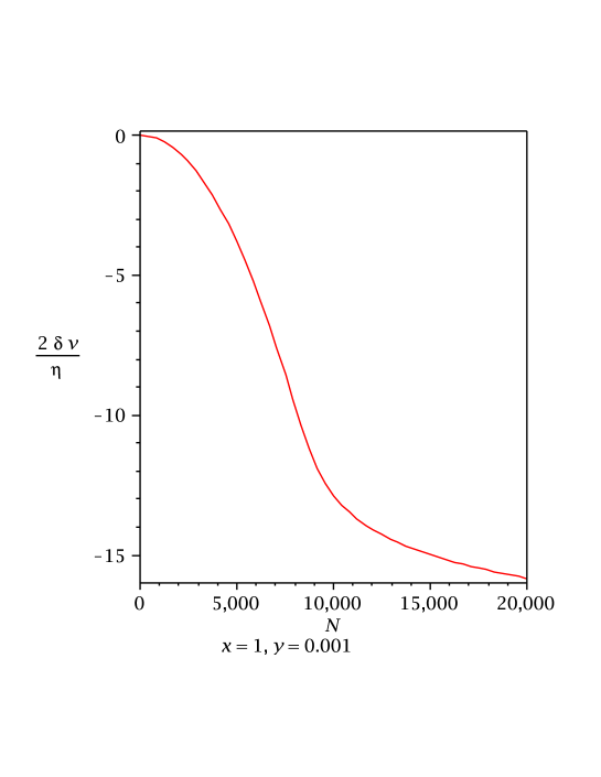
Figure 2: Plot of $\frac{2\delta v}{\eta}$ against $N$

2.4 Backreaction

Our result (2.78) about the 1-loop corrected Hubble parameter is based on perturbative quantum field theory in a (fixed) de Sitter background. Since $H$ changes with time, our computation is valid only if the background is changing not too rapidly so that one can trust the quantum field theory computation. One may introduce the “slow roll parameter”

$$\upvarepsilon:=\frac{d}{dt}H^{-1}$$ (2.89)

as in the inflationary scenario. Here $t$ is the time in the tree level string frame metric (2.21). Note that $\upvarepsilon$ may also be written as

$$\upvarepsilon=\frac{d\ln H}{d{\cal N}},$$ (2.90)

where $d{\cal N}:=Hdt$ measures the number of e-folding. In this representation, $\upvarepsilon$ measures the fractional change of the Hubble parameter per e-folding. Obviously we want $\upvarepsilon\ll 1$ in order for our perturbative computation to be trustable. However this is not the only requirement. We also want the accelerative change of the metric to be small since this effect would backreact directly on the solution through the Einstein equation. Following standard inflation, let us introduce the parameter

$$\upeta:=\frac{d\ln\upvarepsilon}{d{\cal N}},$$ (2.91)

which measure the fractional change of $\upvarepsilon$ per e-folding. In general we need

$$\upvarepsilon,\upeta\ll 1$$ (2.92)

in order to trust the quantum field theory computation.

It is easy to compute $\upvarepsilon$ and $\upeta$ for our model. Substituting (2.71) and (2.78), we obtain

$$\upvarepsilon=\frac{3}{2\sqrt{6}\pi^{2}}\cdot\frac{Ny\sqrt{W(z)}}{1+W(z)}$$ (2.93)

and

$$\upeta=\frac{1}{\sqrt{{\cal R}}}\Big{(}\frac{1}{N}+\frac{W(z)(1-W(z))}{(1+W(z))^{2}}\cdot\frac{3y^{2}}{\pi x^{2}}\Big{)}.$$ (2.94)

An interesting feature of (2.93) and (2.94) is that, given $x$ and $y$, $\upvarepsilon$ and $\upeta$ stay very small for a large range of $N$ from the initial time, and then increase rapidly at around $N$ of the order of $N\sim xy^{-1}\ln y^{-1}$. Typical plots of $\upvarepsilon$ and $\upeta$ against $N$ are shown in the figures 4 and 4

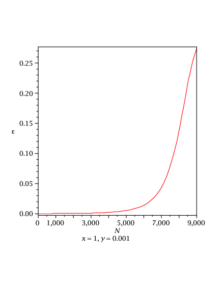
Figure 3: Plot of $\upvarepsilon$ against $N$

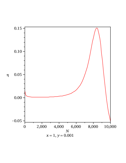
Figure 4: Plot of $\upeta$ against $N$

We emphasis that the parameters $\upvarepsilon$ and $\upeta$ introduced above are defined with respect to the string frame Hubble parameter. In the next section, we will go to the Einstein frame and show that time dependent effect (2.71) of the vev leads to an inflationary cosmology whose slow roll parameters $\upvarepsilon_{E}$, $\upeta_{E}$ are small and resembles those of the standard slow roll inflationary model.

3 Gravitational IR-Effect Driven Inflation

3.1 Einstein frame Hubble constant

To examine the physical significance of the time dependent shift $\delta v$ of the vev of the dilaton, let us go to the Einstein frame. If we denote by $\varphi$ the dynamical part of $\phi$ above the vev,

$$\phi=v_{\rm eff}+\varphi,$$ (3.1)

then in order to decouple the dilaton field $\varphi$ from the Hilbert-Einstein term, we may consider a Weyl scaling of the metric of the form

$${g}_{\mu\nu}=g^{E}_{\mu\nu}e^{2(\frac{\varphi}{\eta}+\beta)},$$ (3.2)

where $\beta$ is an arbitrary function that is independent of the dilaton field $\varphi$. Using (3.2), the scalar curvature $R$ in the string frame can be written in terms of $g^{E}_{\mu\nu}$ and $\varphi$ as

$$R=e^{-2(\frac{\varphi}{\eta}+\beta)}\left[R_{E}-6g_{E}^{\mu\nu}\partial_{\mu}(\frac{\varphi}{\eta}+\beta)\partial_{\nu}(\frac{\varphi}{\eta}+\beta)-6\square_{E}(\frac{\varphi}{\eta}+\beta)\right],$$ (3.3)

and the action in the Einstein frame is

$$S_{E} = \int\sqrt{-{g_{E}}}d^{4}x\left[\frac{M^{2}}{2}e^{2(\beta-\frac{v_{\rm eff}}{\eta})}\Big{(}R_{E}-6g_{E}^{\mu\nu}\partial_{\mu}(\frac{\varphi}{\eta}+\beta)\partial_{\nu}(\frac{\varphi}{\eta}+\beta)-6\square_{E}(\frac{\varphi}{\eta}+\beta)\Big{)}\right.$$ (3.4)

$$\qquad\left.-V(\phi)e^{4(\frac{\varphi}{\eta}+\beta)}-\frac{1}{2}e^{2(\frac{\varphi}{\eta}+\beta)}{g}_{E}^{\mu\nu}\partial_{\mu}(\varphi+v_{\rm eff})\partial_{\nu}(\varphi+v_{\rm eff})\right].$$

Note that spatial dependence in $\beta$ would lead the de Sitter solution (2.77) to an inhomogeneous background metric in the Einstein frame. As we are interested in homogeneous metric as the cosmological description of the universe, so we will not consider spatial dependent $\beta$. This gives the scale factor in the Einstein frame

$$a_{E}(\tau)=a_{0}(\tau)e^{-\frac{\delta v}{\eta}-\beta}$$ (3.5)

where $a_{0}(\tau)$ is given by (2.77). We can also read off from (3.4) the Planck mass

$$M_{P}=Me^{\beta-\frac{v_{\rm eff}}{\eta}}.$$ (3.6)

To compute the Hubble parameter

$$H_{E}=\frac{1}{a_{E}}\frac{da_{E}}{dt_{E}},$$ (3.7)

we note that

$$dt_{E}=e^{-(\beta+\frac{\delta v}{\eta})}dt$$ (3.8)

as a result of the background Einstein metric

$$ds_{E}^{2}=e^{-2(\beta+\frac{\delta v}{\eta})}(-dt^{2}+a_{0}^{2}d{\bf x}^{2}).$$ (3.9)

We obtain

$$H_{E}=e^{\frac{\delta v}{\eta}+\beta}(H_{0}-\frac{d\beta}{dt}-\frac{1}{\eta}\frac{d\delta v}{dt}).$$ (3.10)

In particular, we have

$$H_{E}=e^{\frac{\delta v}{\eta}+\beta}H_{0},\quad\mbox{if}\quad\dot{\beta},\;\frac{1}{\eta}\delta\dot{v}\ll H_{0}.$$ (3.11)

As we will see later, this is the case of interest and relevance to us.

It is instructive to note that the relation (3.11) may also be understood using the Friedmann equation

$$H_{E}^{2}=\frac{U}{3M_{P}^{2}}$$ (3.12)

where $U$ denotes the energy density for the 1-loop corrected vacuum $\phi=v_{\rm eff}$, i.e. $\varphi=0$. By putting $\varphi=0$ in (3.4), we obtain

$$U=e^{4\beta}\Big{[}V(v_{\rm eff})+3M^{2}e^{-\frac{2v}{\eta}}\Big{(}(\frac{d\beta}{dt})^{2}-\frac{1}{a_{0}^{3}e^{-\frac{2\delta v}{\eta}}}\frac{d}{dt}(a_{0}^{3}e^{-\frac{2\delta v}{\eta}}\frac{d\beta}{dt})\Big{)}-\frac{1}{2}e^{\frac{2\delta v}{\eta}}(\frac{d\delta v}{dt})^{2}\Big{]}$$ (3.13)

where we have used the background Einstein metric (3.9). This gives the Hubble parameter

$$H_{E}^{2}=e^{2(\beta+\frac{\delta v}{\eta})}\big{(}H_{0}^{2}+(\frac{d\beta}{dt})^{2}+\cdots\big{)},$$ (3.14)

where $\cdots$ denotes contributions obtained from the third and fourth term in (3.13). The two terms listed above resemble those one would obtain from (3.10). However the $\cdots$ terms are completely different. The reason for the discrepancy is simple: the expression (3.13) is not the correct vacuum energy density for the state $\phi=v+\delta v$ as it was obtained from the tree level Einstein action without taking into full account of the 1-loop IR effects. Turning the argument around, we can use the Friedmann equation to obtain the vacuum energy density,

$$U=e^{4\beta}(V(v)+\delta V)\Big{(}1-\frac{1}{H_{0}}\frac{d\beta}{dt}-\frac{1}{H_{0}\eta}\frac{d\delta v}{dt}\Big{)}^{2},$$ (3.15)

where $\delta V$ denotes the 1-loop corrections, both UV and IR, to $V$. As we discussed above, UV corrections are time independent. Typically, $\delta V$ receives a contribution of order $\Uplambda_{UV}^{4}$ from the zero point energy fluctuation. This term is much bigger than the other UV or IR corrections to the potential. So the dominant time dependence comes from the exponential prefactor and one recovers immediately (3.11).

A couple of remarks follows.

1. So far $\beta$ is general. While the relations (3.6), (3.11) generally depend on $\beta$, the ratio

   $$\frac{H_{E}}{M_{P}}=\frac{H_{0}}{Me^{-v/\eta}}e^{2\delta v/\eta}$$ (3.16)

   is independent of the choice of the frame and thus is an useful quantity to ask physical question about it.

2. In the literature, IR effects of the graviton loops have been studied rather extensively in various setting and models. The exponentiation of the IR effects of the graviton loops (3.16) is new and is the main finding of this paper. Note that $\delta v$ is always negative for $\eta>0$ so we always get an exponential suppression/screening on the cosmological constant. In general, the longer the elapsed time, the greater will be the screening.

3. In the above analysis, we did not take into account of the quantum gravity corrections to the classical Einstein equation. This is a difficult problem since quantized gravity effect in de Sitter background is poorly understood in general. An embedding in string theory does not help in this case since string theory in time dependent background has met with a number of conceptual as well as technical difficulties. Due to a lack of reliable mean to compute these quantum corrections, we will ignore this issue in our current discussion.

3.2 Slow roll inflation from gravitational IR-effect

$M_{P}$ is time dependent for general $\beta$. Although it is an interesting scenario to consider a time dependent Newton constant, and it can indeed be easily accommodated in our framework, however given that it is not yet universally accepted that such a variation does exist , we will not consider this possibility in this paper. Let us therefore consider the choice of frame with

$$\beta=\frac{\delta v}{\eta}.$$ (3.17)

In this frame, we have a constant Planck scale

$$M_{P}=Me^{-v/\eta}.$$ (3.18)

This gives not just the natural UV cut off scale of the Einstein frame action, but also the UV cutoff scale $\Uplambda_{\rm UV}$ of the string frame action (2.1) in the presence of vev (2.8). As it is easy to check that $\eta^{-1}d\delta v/dt\ll H_{0}$ is satisfied, therefore the Hubble parameter acquires a time variation of the form

$$H_{E}=H_{0}e^{\frac{2\delta v}{\eta}}$$ (3.19)

from the graviton IR loop effect. In this frame, $H_{0}$ is also the initial value of the Einstein frame Hubble parameter. Note that generally one may consider a change of frame by adding to (3.17) an arbitrary constant and still obtain a time independent Planck mass. This would modify the definition (3.18) of $M_{P}$ with a multiplicative constant factor. However this is a physically equivalent frame since physics is unchanged if we express everything in terms of $M_{P}$.

As $\delta v<0$, the Einstein frame metric describes an inflationary cosmology with a Hubble parameter (3.19) that is decreasing in magnitude with time. The slow roll parameters,

$$\upvarepsilon_{E}:=\frac{d}{dt_{E}}H_{E}^{-1},\quad\upeta_{E}:=\frac{1}{H_{E}\upvarepsilon_{E}}\frac{d\upvarepsilon_{E}}{dt_{E}}$$ (3.20)

are given by

$$\upvarepsilon_{E}=2e^{\frac{\delta v}{\eta}}\upvarepsilon,\quad\upeta_{E}=e^{\frac{\delta v}{\eta}}(\upeta-\upvarepsilon)$$ (3.21)

for our model. We note that $N$, as defined in (2.83) above, is in fact equal to the number of e-folding ${\cal N}_{E}$ in the Einstein frame $d{\cal N}_{E}:=H_{E}dt_{E}$:

$${\cal N}_{E}=N.$$ (3.22)

That this is true independent of the choice of $\beta$ can be seen immediately from (3.8) and (3.11). Due to the presence of the suppression factor $\exp{\frac{\delta v}{\eta}}<1$, the Einstein slow roll parameters will be small as long as the $\upvarepsilon,\upeta$ are small. Since the later parameters control the backreaction to the quantum field computation performed in the string frame, therefore as long as we are in a regime of parameters (2.92) that we can trust the quantum field theory computations, the corresponding cosmology in the Einstein frame describes a slow roll inflation with

$$\upvarepsilon_{E},\upeta_{E}\ll 1.$$ (3.23)

A couple of remarks are in order.

1. In discussing the cosmological consequences of any QFT calculation, it is important to employ an observable that is gauge invariant. In the above, we have used the time dependent IR effects of the vev of the dilaton scalar field to deduce the existence of a screening effect on the cosmological constant. In a gauge theory, the quantum corrected effective potential is generally gauge dependent. While it does not necessarily mean that the vev of the scalar field, as can be determined equivalently from the effective potential, is also gauge dependent, it is necessary to check whether this is the case. If it is so, it will be interesting to replace the vacuum expectation value of the scalar field with a gauge invariant order parameter and redo the analysis of this paper. Lessons learnt in a previous analysis [62] may be useful.

2. In the simplest model of inflation, inflationary expansion is driven by the slow rolling of an inflaton field down an almost flat potential as in the slow roll inflation model. In our model, inflationary expansion is driven by a different mechanism, the IR effects of the gravitons themselves. Slow roll inflation is achieved without a slow roll potential.

3. One of the obstacles in the slow roll model of inflation is that why is the inflaton mass so light. Expressed in terms of the eta parameter, it is required that

   $$\upeta_{E}=\frac{m_{\phi}^{2}}{3H_{E}^{2}}\ll 1.$$ (3.24)

   Like the Higgs hierarchy problem, generically

   $$m_{\phi}^{2}\sim\Uplambda_{\rm UV}^{2}\gg H_{E}^{2}.$$ (3.25)

   Supersymmetry improves it a little since contributions from bosons and fermions cancel precisely. However supersymmetry is spontaneously broken during inflation and this leads to an inflaton mass of order Hubble

   $$m_{\phi}^{2}\sim H_{E}^{2}.$$ (3.26)

   and $\upeta$ is of order one. The presence of large quantum corrections to the eta parameter simply ruins the inflationary picture predicted by the classical potential.

   In our model, the dilaton field is sitting at the minimum of the quantum corrected effective potential. Change of vacuum energy is not due to a rolling of the dilaton field as in model with an inflaton, but is due to the time dependent IR effect of graviton loops on the position of the minimum. It is all right for $m_{\phi}^{2}$ to receive large UV corrections, but these are time independent and does not change the results of our model. For example, the value of $H_{0}$ will depend on the UV cutoff of the theory, but the time dependence in (3.19) is not as it arises from IR quantum corrections. In order words, unlike the slow roll model, our model is free from the eta problem and we can trust the time evolution of the Hubble parameter.

3.3 Screening of the cosmological constant

In the history of universe, there has been at least two regimes of de Sitter phases, one is the inflation era in the early universe, the other is the expansion of the current universe which is described by an de Sitter metric in the asymptotic future. For the inflationary phase, the inflation scale is constrained by the Planck observation [63] of the amplitude of the CMB power spectrum to be

$$H_{E,{\rm inf}}\sim(\frac{r}{0.01})^{1/2}\times 10^{14}{\rm GeV},$$ (3.27)

where $r$ is the tensor-to-scalar ratio. For concreteness, let us consider the case of $r\sim 0.01$ and so

$$H_{E,{\rm inf}}\sim 10^{14}{\rm GeV}.$$ (3.28)

One of the interesting question about inflation is what set the scale of inflation $H_{E,{\rm inf}}$? We can use (3.19) to address this. In the usual picture about quantum gravity, spacetime is highly quantized right after the big bang. After about one unit of Planck time, classical geometry begins to make sense. Let us consider the situation where inflation started at about this time. In this case, it is natural to take the initial condition that the initial value of the Hubble parameter is given by the Planck mass

$$H_{E}(0)=M_{P}.$$ (3.29)

This corresponds to $x=1$. After expanding with a number $N$ of e-folding, the Hubble parameter is given by

$$H_{E}(N)=M_{P}\;{\cal R},$$ (3.30)

where ${\cal R}$, as given by the (2.80), determines the amount of screening. We have thus found that the de Sitter symmetry breaking IR loop effects provide a screening of the cosmological constant. Screening of the cosmological constant due to IR effects of gravity has been conjectured and argued for long ago. Our model provides a concrete set up where the screening mechanism and its effects can be calculated reliably.

For a given model, $M,v$ and $\eta$ are given. Equivalently we can use the Planck mass $M_{P}$, which set the scale, and the dimensionless parameters $x,y$ of (2.82) to specify the model. As long as the parameters (2.92) are small, it is easy to accommodate (3.28) with an amount

$${\cal R}=10^{-4}$$ (3.31)

of screening. In Table 1, we show for $x=1$ and different values of $y$, the values of $N$, $\upvarepsilon$ and $|\upeta|$ giving ${\cal R}=10^{-4}$.

$y$	$N$	$\upvarepsilon$	$|\upeta|$
$1$	$628$	$0.16$	$6\times 10^{-7}$
$0.01$	$1000$	$0.22$	$0.06$
$0.0001$	$77850$	$0.012$	$0.013$

Table 1: The values of $N$, $\upvarepsilon$ and $|\upeta|$ giving ${\cal R}=10^{-4}$ for $x=1$ and different values of $y$.

In practice we want to achieve this amount of screening before inflation ends. This is the point where $\upvarepsilon_{E}=1$. One can play with the parameters $x,y$ and it is not hard to convince oneself that our $\upvarepsilon_{E}$ can never exceed 1. What it means is the IR effect of graviton loops on the vev is not sufficient to end inflation; and we need a new effect to change the behavior of the Hubble parameter so that $\frac{d}{dt_{E}}(a_{E}H_{E})^{-1}$ change sign. What could this effect be?

In the simplest slow roll inflation model, inflation ends when the inflaton potential steepens (large $V^{\prime}$) and the inflaton field picks up kinetic energy. After inflation end, the inflaton starts to oscillate around the global minimum of the potential and the energy of the inflaton field is transferred to the standard model sector through a decay of the inflaton field to the standard model particles. In the scenario described above, the universe started to inflate right after or soon after big bang, with a Planck scale Hubble parameter initially. The IR loop effect of the graviton generates a screening on the Hubble parameter which resembles the slow roll feature of the flat potential in slow roll inflation model. In order to be able to transfer the energy stored in the dilaton to the standard model matter fields, we assume that the dilaton is coupled to the standard model field $\psi$, for example

$${\cal L}_{\rm int}=\lambda\phi\bar{\psi}\psi,$$ (3.32)

Now $\lambda$ determines the rate of decay of the inflaton to the standard model particles, $\phi\to\bar{\psi}\psi$, and this has a effect of decreasing the Hubble parameter. This effect is usually small, but in our model, one can expect that the coupling $\lambda$ will also receive de Sitter symmetry breaking IR corrections and becomes time dependent . It is possible that $\lambda(t)$ may become strong as time evolves and effectively playing the role of a steepened potential and ends the inflation. This is an interesting scenario and will be the subject of a separate paper.

As for the current universe, the current value of the Hubble constant $H_{E,{\rm now}}\simeq 10^{-42}{\rm GeV}$ is tiny. In terms of the Planck mass $M_{P}=10^{18}{\rm GeV}$, it is

$$H_{E,{\rm now}}\simeq 10^{-60}M_{P},$$ (3.33)

or in terms of the cosmological constant $\Lambda_{E}=3H_{E}^{2}$:

$$\Lambda_{E,{\rm now}}\simeq 10^{-120}M_{P}^{2}.$$ (3.34)

The original cosmological constant problem is to understand why the current cosmological constant is so much smaller than $M_{P}^{2}$, the natural value of the vacuum energy in a generic setting. Supersymmetry helps a little but we still get a large hierarchy to explain. We will have nothing to say about this problem except to say that in our model the Hubble parameter is a function of time whose history is determined by the dynamics of the theory and the initial condition, e.g. (3.29). A proper understanding of the process of reheating is needed in order to understand what value the cosmology constant take after reheating. This would serve as the initial condition of the Hubble parameter which then evolve to the small value it takes nowadays.

4 Conclusion and Discussion

In this paper, we have considered an effective theory of gravity with which a dilaton field is coupled exponentially to. We found that the 1-loop IR effects of the gravitons break the de Sitter symmetry of the background, and constitute a time dependent contribution to the vev of dilaton field. We note that, in the Einstein frame, this time dependent effect is exponentiated and acts to reduce the cosmological constant over time. This provides a concrete mechanism of screening of the cosmological constant through the IR effects of the graviton.

To determine the late time behaviour of the system, we employ the DRG method to re-sum the leading IR logarithms. This allows us to follow the effects of the screening on the cosmological evolution of the universe. In particular, we find that one can have an inflation scenario driven entirely by the gravitational IR effect. This IR-driven inflation achieves all the standard features of the slow roll inflation model such as having a slowing changing Hubble constant (small slow roll parameters ) and sufficient amount of e-foldings etc. Moreover, since the UV divergence of the theory is time independent and does not mix, at least in the 1-loop order, with the time dependent IR effects; as a consequence, our model does not suffer from the eta problem that baffles models with inflation driven by an inflaton potential.

To discuss the ending of inflation and reheating in our model, it is necessary to include in our model the coupling of the dilaton field to matter fields. We speculated that the IR effect on the dilaton-matter coupling may acts effectively like a damping term and provide a mechanism for the ending and reheating of the inflation.

The dilaton-gravity sector of our model is specified by the Planck mass scale and two dimensionless parameters, ratio of initial Hubble constant with respect to the Planck mass, and the ratio of the dilaton gravity coupling constant with respect to the Planck mass. It is interesting to study the other signatures of the model, such as the tensor scalar ratio $r$, the primordial non-Gaussanity $f_{NL}$ and the tilt and other features of the power spectrum.

There is compelling evidence that the universe is presently undergoing a period of accelerated expansion and the expansion is supported by some form of dark energy. However the nature of dark energy is mysterious and it is not known whether it is a cosmological constant or something else. If it is given by some form of quintessence, the kind of IR loop effects we studied in this paper will exist and may play a role and leave signature on the late time cosmology.

Our analysis is based on 1-loop UV and IR effects, improved by a resumation of the leading IR logarithms. At higher loop orders, UV divergences may mix with the IR divergences and leads to new effects. This however will depend on the UV completion of the effective theory. This is one way how Planckian suppressed corrections may become relevant and how UV sensitivity maybe regained in our model.

Appendix A Interaction Terms of Gravitons and the Dilaton

In this appendix, we give the interaction terms of the graviton and the dilaton. In this article, we need only the three-point vertices, $hh{\hat{\phi}}$ and ${\hat{\omega}}{\hat{\omega}}{\hat{\phi}}$, to calculate the 1-loop tadpole diagrams generated by the graviton loop. For completeness, we list also the interaction terms up to cubic order in the graviton perturbations, $h_{\mu\nu}$ and $\omega$, and quintic order in the scalar perturbation ${\tilde{\phi}}$, which may be useful for other applications of our model.

Our total interaction Lagrangian is given by

$${\cal L}_{\rm int}={\cal L}_{1}+{\cal L}_{2}+{\cal L}_{3},$$ (A.1)

where

$${\cal L}_{1} = \frac{M^{2}}{2}\sqrt{-g}e^{-\phi/\eta}R,$$ (A.2)

$${\cal L}_{2} = -\frac{1}{2}\sqrt{-g}g^{\mu\nu}\partial_{\mu}\phi\partial_{\nu}\phi,$$ (A.3)

$${\cal L}_{3} = -\sqrt{-g}V(\phi).$$ (A.4)

Presented according to the order of the order of graviton fluctuations, we have:

(1) Zeroth order in $h$ and $\omega$:

$$\frac{8\kappa^{2}}{H_{0}^{2}a_{0}^{4}}{\cal L}_{1}^{(0)} = -\frac{2}{\eta^{3}}\zeta^{3}{\hat{\phi}}^{3}+\frac{1}{\eta^{4}}\zeta^{4}{\hat{\phi}}^{4},$$ (A.5)

$${\cal L}_{2}^{(0)} = 0,$$ (A.6)

$$\frac{1}{a_{0}^{4}}{\cal L}_{3}^{(0)} = -\frac{\xi}{6}\zeta^{3}{\hat{\phi}}^{3}-\frac{\lambda}{24}\zeta^{4}{\hat{\phi}}^{4},$$ (A.7)

where

$$\xi:=V^{(3)}(v),\quad\lambda:=V^{(4)}(v)$$ (A.8)

and we have used

$${\tilde{\phi}}=\zeta{\hat{\phi}}.$$ (A.9)

(2) Linear order in $h$ and $\omega$:

$$\frac{\kappa}{2a_{0}^{2}}{\cal L}_{1}^{(1)} = \left[\partial_{\rho}\partial_{\nu}h^{\rho\nu}-\frac{6}{\tau}\partial_{\rho}h^{\rho 0}+\frac{12}{\tau^{2}}h^{00}-6\partial_{\mu}\partial^{\mu}{\hat{\omega}}-\frac{12}{\tau}\partial_{0}{\hat{\omega}}+\frac{24}{\tau^{2}}{\hat{\omega}}\right.$$ (A.10)

$$\left.-\frac{6\zeta}{\kappa\eta}\left(\partial_{\mu}\partial^{\mu}{\hat{\phi}}+\frac{2}{\tau}\partial_{0}{\hat{\phi}}-\frac{4}{\tau^{2}}{\hat{\phi}}\right)\right]\left(\frac{\zeta^{2}}{\eta^{2}}{\hat{\phi}}^{2}-\frac{2}{3}\frac{\zeta^{3}}{\eta^{3}}{\hat{\phi}}^{3}+\frac{1}{3}\frac{\zeta^{4}}{\eta^{4}}{\hat{\phi}}^{4}\right),$$

$$-\frac{2}{\kappa\zeta^{2}a_{0}^{2}}{\cal L}_{2}^{(1)} = \partial_{\mu}{\hat{\phi}}\partial_{\nu}{\hat{\phi}}\left(2{\hat{\omega}}\eta^{\mu\nu}+\frac{2\zeta}{\kappa\eta}{\hat{\phi}}\eta^{\mu\nu}-h^{\mu\nu}\right),$$ (A.11)

$$-\frac{1}{4\kappa a_{0}^{4}}{\cal L}_{3}^{(1)} = \left({\hat{\omega}}+\frac{\zeta}{\kappa\eta}{\hat{\phi}}\right)\left(\frac{\sigma^{2}}{2}\zeta^{2}{\hat{\phi}}^{2}+\frac{\xi}{6}\zeta^{3}{\hat{\phi}}^{3}+\frac{\lambda}{24}\zeta^{4}{\hat{\phi}}^{4}\right).$$ (A.12)

(3) Quadratic order in $h$ and $\omega$.

$$\frac{1}{a_{0}^{2}}{\cal L}_{1}^{(2)} = \left[{\underline{-\frac{1}{4}\partial_{\mu}h_{\rho\sigma}\partial^{\mu}h^{\rho\sigma}-\frac{1}{2}\partial_{\mu}(h^{\mu}_{\ \rho}\partial_{\nu}h^{\rho\nu})-\frac{1}{2}h^{\mu}_{\ \rho}\partial_{\mu}\partial_{\nu}h^{\rho\nu}+2{\hat{\omega}}\partial_{\mu}\partial_{\nu}h^{\mu\nu}}}\right.$$ (A.13)

$${\underline{+6\partial_{\mu}(h^{\mu\nu}\partial_{\nu}{\hat{\omega}})-\frac{12}{\tau}\partial_{\mu}(h^{0\mu}{\hat{\omega}})+\frac{3}{\tau}\ \partial_{\mu}(h^{0\nu}h_{\nu}^{\ \mu})-\frac{6}{\tau^{2}}h^{\rho 0}h_{\rho}^{\ 0}+\frac{24}{\tau^{2}}h^{00}{\hat{\omega}}}}$$

$${\underline{-6\partial_{\mu}({\hat{\omega}}\partial^{\mu}{\hat{\omega}})-6{\hat{\omega}}\partial_{\mu}\partial^{\mu}{\hat{\omega}}-\frac{24}{\tau}{\hat{\omega}}\partial_{0}{\hat{\omega}}+\frac{24}{\tau^{2}}{\hat{\omega}}^{2}}}$$

$$-\frac{6\zeta}{\kappa\eta}\left(-\frac{1}{3}{\hat{\phi}}\partial_{\mu}\partial_{\nu}h^{\mu\nu}-\partial_{\mu}(h^{\mu\nu}\partial_{\nu}{\hat{\phi}})+\frac{2}{\tau}\partial_{\mu}(h^{0\mu}{\hat{\phi}})-\frac{4}{\tau^{2}}h^{00}{\hat{\phi}}+{\hat{\phi}}\partial_{\mu}\partial^{\mu}{\hat{\omega}}\right.$$

$$\quad\qquad\left.+{\hat{\omega}}\partial_{\mu}\partial^{\mu}{\hat{\phi}}+\partial_{\mu}({\hat{\phi}}\partial^{\mu}{\hat{\omega}}+{\hat{\omega}}\partial^{\mu}{\hat{\phi}})+\frac{4}{\tau}{\hat{\phi}}\partial_{0}{\hat{\omega}}+\frac{4}{\tau}{\hat{\omega}}\partial_{0}{\hat{\phi}}-\frac{8}{\tau^{2}}{\hat{\omega}}{\hat{\phi}}\right)$$

$$\left.-\frac{6\zeta^{2}}{\kappa^{2}\eta^{2}}\left(\partial_{\mu}({\hat{\phi}}\partial^{\mu}{\hat{\phi}})+{\hat{\phi}}\partial_{\mu}\partial^{\mu}{\hat{\phi}}+\frac{4}{\tau}{\hat{\phi}}\partial_{0}{\hat{\phi}}-\frac{4}{\tau^{2}}{\hat{\phi}}^{2}\right)\right]$$

$$\times\left({\underline{-\frac{2\zeta}{\eta}{\hat{\phi}}}}+\frac{\zeta^{2}}{\eta^{2}}{\hat{\phi}}^{2}-\frac{2\zeta^{3}}{3\eta^{3}}{\hat{\phi}}^{3}+\frac{\zeta^{4}}{3\eta^{4}}{\hat{\phi}}^{4}\right),$$

$$-\frac{4}{\kappa^{2}\zeta^{2}a_{0}^{2}}{\cal L}_{2}^{(2)} = \partial_{\mu}{\hat{\phi}}\partial_{\nu}{\hat{\phi}}\left[h^{\mu\rho}h_{\rho}^{\ \nu}+4\eta^{\mu\nu}{\hat{\omega}}^{2}-4h^{\mu\nu}{\hat{\omega}}+\frac{4\zeta}{\kappa\eta}\Big{(}2\eta^{\mu\nu}{\hat{\omega}}{\hat{\phi}}-h^{\mu\nu}{\hat{\phi}}+\frac{\zeta}{\kappa\eta}\eta^{\mu\nu}{\hat{\phi}}^{2}\Big{)}\right],$$

(A.14)

$$-\frac{1}{8\kappa^{2}a_{0}^{4}}{\cal L}_{3}^{(2)} = \Big{(}{\underline{{\hat{\omega}}^{2}}}+\frac{2\zeta}{\kappa\eta}{\hat{\omega}}{\hat{\phi}}+\frac{\zeta^{2}}{\kappa^{2}\eta^{2}}{\hat{\phi}}^{2}\Big{)}\Big{(}{\underline{\rho\zeta{\hat{\phi}}}}+\frac{\sigma^{2}}{2}\zeta^{2}{\hat{\phi}}^{2}+\frac{\xi}{6}\zeta^{3}{\hat{\phi}}^{3}+\frac{\lambda}{24}\zeta^{4}{\hat{\phi}}^{4}\Big{)}.$$ (A.15)

In deriving (A.10) – (A.15) we have used (2.29). The underlined terms in the above formula correspond to the vertices of the one-loop tadpole diagrams investigated in section 2.3.

Appendix B Comments on the IR Divergence of Two-Point Function

B.1 de Sitter space

It is instructive to comment on the origin of time dependent de Sitter symmetry breaking term in the propagator of a massless minimally coupled scalar field. The mode expansion for a massless minimally coupled scalar in de Sitter background in the Bunch-Davies vacuum is given by

$$\chi=\frac{1}{(2\pi)^{3/2}a_{0}(\tau)}\int d^{3}p\;[a_{{\bf p}}e^{i{{\bf p}}\cdot{{\bf x}}}\chi_{p}(\tau)+{\rm h.c.}],\quad\chi_{p}(\tau)=\frac{1}{\sqrt{2p}}\left(1-\frac{i}{p\tau}\right)e^{-ip\tau}.$$ (B.1)

From this we obtain the propagator

$$\langle\chi(x)\chi(x^{\prime})\rangle=\int\frac{d^{3}p}{(2\pi)^{3}}\frac{H_{0}^{2}\tau\tau^{\prime}}{2p}\left(1-\frac{i}{p\tau}\right)\left(1+\frac{i}{p\tau^{\prime}}\right)e^{-ip(\tau-\tau^{\prime})+i{\bf p}\cdot({\bf x}-{\bf x}^{\prime})}.$$ (B.2)

The propagator has UV as well as IR divergences. The UV divergence reflects the fact that the considered Lagrangian is a valid effective description only down to a certain physical distance scale $\ell$ and the divergence can be regulated by imposing a cutoff

$$P\leq\Uplambda_{\rm UV}:=\frac{1}{\ell}$$ (B.3)

on the physical momentum $P:=p/a_{0}(t)$. The IR divergence

$$\langle\chi(x)\chi(x^{\prime})\rangle_{\rm IR}\sim\int_{0}\frac{d^{3}P}{(2\pi)^{3}}\frac{H_{0}^{2}}{2P^{3}},$$ (B.4)

on the other hand, is due to legitimate physical effects occurring at very long distances. In the present case of a de Sitter background, assume that initially the universe has a physical size $L_{0}$ where the different parts of the universe were in causal contact, then a sensible IR regulator is to put the universe in a box of size $L(t)=a_{0}(t)L_{0}$. This cuts out contributions from distance scale larger than those that can be related by causal effects. In terms of physical momentum, this corresponds to a cutoff

$$P\geq P_{\rm min}:=\frac{1}{a_{0}(t)L_{0}}.$$ (B.5)

We emphasize that, unlike the IR regulator whose time dependence is dedicated by the associated physics, the UV regulator (B.3) is independent of time, and so UV divergences are taken care of by the standard UV renormalization techniques. In contrast, IR divergences give rise to time growing de Sitter symmetry breaking effect in the theory. The same time dependent factor also arises in the graviton propagator.

B.2 Power law Friedmann-Robertson-Walker metric

The result (B.4) about IR divergence can be easily generalized to the more general case of a spatially flat Friedmann-Robertson-Walker metric

$$ds^{2}=-dt^{2}+a_{0}^{2}(t)d{\bf x}^{2},$$ (B.6)

with a power-law scale factor [64, 21]

$$a_{0}(t)=wt^{c}\quad\mbox{where $w$ and $c$ are constants}.$$ (B.7)

Note that $c=\frac{1}{2}$ corresponds to radiation dominated era, $c=\frac{2}{3}$ corresponds to matter dominated era, and $c\to\infty$ corresponds to de Sitter space [64]. A minimally coupled massless scalar in this metric has the equation of motion

$$-a_{0}^{-3}\partial_{t}(a_{0}^{3}\partial_{t}\chi)+a_{0}^{-2}\partial_{i}^{2}\chi=0.$$ (B.8)

Let us introduce the conformal time $\tau$ defined by (for $c\neq 1$),

$$\tau:=\int^{t}\frac{dt^{\prime}}{a_{0}(t^{\prime})}=\frac{1}{(1-c)w}t^{1-c}.$$ (B.9)

In terms of $\tau$, the scale factor can be written as

$$a_{0}=k\tau^{\frac{c}{1-c}},\quad k=w[w(1-c)]^{\frac{c}{1-c}}$$ (B.10)

and the field equation becomes

$$\partial_{\tau}(a_{0}^{2}\partial_{\tau})\chi-a_{0}^{2}\partial_{i}^{2}\chi=0.$$ (B.11)

The mode function $\chi_{p}$ of $\chi$:

$$\chi=\frac{1}{(2\pi)^{3/2}a_{0}(\tau)}\int d^{3}p\;[a_{{\bf p}}e^{i{{\bf p}}\cdot{{\bf x}}}\chi_{p}(\tau)+{\rm h.c.}]$$ (B.12)

can be solved exactly in terms of the Hankel functions,

$$\chi_{p}=c_{1}(p)\;\tau^{\frac{1}{2}}H^{(1)}_{\nu}(p\tau)+c_{2}(p)\tau^{\frac{1}{2}}H^{(2)}_{\nu}(p\tau)$$ (B.13)

where

$$b:=\frac{1-c}{1-3c},\quad\nu:=\frac{1}{|2b|}>0.$$ (B.14)

Canonical quantization constraints the coefficients $c_{1}$ and $c_{2}$ to satisfy the normalization condition

$$\chi_{p}\frac{d\chi_{p}^{*}}{d\tau}-\chi_{p}^{*}\frac{d\chi_{p}}{d\tau}=i.$$ (B.15)

This gives

$$|c_{2}|^{2}-|c_{1}|^{2}=\frac{\pi}{4}$$ (B.16)

A convenient parametrization of the solution is

$$c_{1}=\sqrt{\frac{\pi}{4}}\sinh\alpha e^{i\beta},\quad c_{2}=\sqrt{\frac{\pi}{4}}\cosh\alpha$$ (B.17)

for real $\alpha$, $\beta$, where we have, for convenience, taken $c_{2}$ to be real and positive. In general an overall phase factor for $c_{1}$ and $c_{2}$ can be inserted but it does not show up in any physical quantity. Thus it is sufficient to consider the two parameters family ($\alpha$,$\beta$). In the de Sitter case, the Bunch-Davis vacuum corresponds to the choice $\alpha=0$. The $\alpha$-vacua is parametrized by ($\alpha$, $\beta$), $\alpha\neq 0$.

For quantum field theory in curved spacetime, it is customary to impose the Hadamard condition which states that the short distance singularity structure of the two point function should be closed to that for the Minkowski space

$$\chi_{p}\sim\frac{1}{\sqrt{2p}}e^{-ip\tau},\quad p\tau\gg 1.$$ (B.18)

Using the asymptotic expansion of the Hankel function for large $z\gg 1$,

$$H^{(1)}_{\nu}(z)\sim\sqrt{\frac{2}{\pi z}}e^{i(z-\pi\nu/2-\pi/4)},\quad H^{(2)}_{\nu}(z)\sim\sqrt{\frac{2}{\pi z}}e^{-i(z-\pi\nu/2-\pi/4)}.$$ (B.19)

we find that the mode function behaves in the high energies limit as

$$a_{0}\chi_{p}\sim\frac{1}{\sqrt{2p}}(c_{1}e^{ip\tau}+c_{2}e^{-ip\tau}),$$ (B.20)

This amounts to the choice of the coefficients:

$$c_{1}=0,\quad|c_{2}|^{2}=\frac{\pi}{4}.$$ (B.21)

We are interested in the IR behaviour of the two point function

$$\langle\chi(x)\chi(x^{\prime})\rangle=\frac{1}{(2\pi)^{3}a_{0}(\tau)a_{0}(\tau^{\prime})}\int d^{3}pe^{i{{\bf p}}\cdot({{\bf x}}-{{\bf x}}^{\prime})}\chi_{p}(\tau)\chi_{p}^{*}(\tau^{\prime}).$$ (B.22)

For small $p$, we use the asymptotic behavior of the Hankel functions (for $\mathop{\rm Re}\nolimits\nu>0$),

$$H_{\nu}^{(1)}(z)\sim-H_{\nu}^{(2)}(z)\sim-\frac{i}{\pi}\Gamma(\nu)(z/2)^{-\nu},\quad z\to 0,$$ (B.23)

then, apart from a constant factor, the small $p$ behavior of the two point function is given by

$$\langle\chi(x)\chi(x^{\prime})\rangle=\mbox{const.}\times\int d^{3}p\frac{|c_{1}-c_{2}|^{2}}{p^{2\nu}}\times\frac{1}{(\tau\tau^{\prime})^{\beta}},$$ (B.24)

where

$$\beta:=\nu-(2b)^{-1}=\begin{cases}2\nu,&\mbox{for $b<0$, \; i.e. $1/3<c<1$},\\ 0,&\mbox{for $b>0$, \; i.e. $c<1/3$ or $c>1$}.\end{cases}$$ (B.25)

We will adopt the Hadamard condition and so (B.21) implies that the two point function acquires an IR divergence from the momentum integration if $|(1-3c)/(1-c)|\geq 3$, i.e.

$$\frac{2}{3}\leq c\leq 1\quad\mbox{or}\quad c>1.$$ (B.26)

Thus apart from the de Sitter space ($c\to\infty$), the scalar two point function is also IR divergent in the matter dominated era $c=2/3$ and hence picks up the same time growing logarithmic factor $\ln(a_{0}(\tau)a_{0}(\tau^{\prime}))$ after an IR cutoff is introduced . However there is an important difference between the two cases: there is an additional time dependent factor $(\tau\tau^{\prime})^{-3}=a_{0}(\tau)^{-3/2}a_{0}(\tau^{\prime})^{-3/2}$ in the case of matter dominated era. This factor actually decreases to zero faster than the growth of the factor $\ln(a_{0}(\tau)a_{0}(\tau^{\prime}))$, therefore we expect that the graviton loop in the matter dominated era does not induces any screening effect in late times.

Appendix C Light Field Condition for the Dilaton

In this appendix we investigate the parameter region from the constraint on the dilaton mass $m_{\hat{\phi}}\ll H^{2}$ which is needed for the approximation of the massive scalar propagator (2.56). Let us recall

$$m_{\hat{\phi}}^{2}=\zeta^{2}\left(\sigma^{2}+\frac{4\rho}{\eta}\right),\quad H_{0}^{2}=\frac{1}{3M^{2}}e^{2v/\eta}V_{0},\quad\rho=-\frac{4V_{0}}{\eta}$$ (C.1)

The condition is written as

$$\frac{m_{\hat{\phi}}^{2}}{H_{0}^{2}}=\zeta^{2}\left(\frac{\sigma^{2}}{H_{0}^{2}}-\frac{48M^{2}}{\eta^{2}}e^{-2v/\eta}\right)\ll 1.$$ (C.2)

For the two terms in the parenthesis to be small separately , we require

$$\frac{16V_{0}}{\eta^{2}}<\sigma^{2}\ll\frac{1}{3M^{2}}e^{2v/\eta}V_{0},\qquad\eta^{2}\gg 48M^{2}e^{-2v/\eta},$$ (C.3)

where the lower bound of $\sigma$ comes from (2.20). At the same time, we have $\zeta\simeq 1$. We find that as long as the second constraint in (C.3) is satisfied, there will be a broad range for $\sigma^{2}$ and (C.2) can be easily satisfied. In terms of the parameter $y$ introduced in (2.82), the second constraint in (C.3) reads

$$y^{2}\ll\frac{1}{48}.$$ (C.4)

In a different way, (C.2) can be satisfied by requiring a balanced cancellation of two terms in the parenthesis in (C.2). This leads to $\sigma\sim 16V_{0}/\eta^{2}$ and will need some fine tuning in this case.

References

• [1]
• [2] S. Kachru, R. Kallosh, A. D. Linde, J. M. Maldacena, L. P. McAllister and S. P. Trivedi, “Towards inflation in string theory,” JCAP 0310 (2003) 013 [hep-th/0308055].
• [3]
• [4] E. Silverstein and D. Tong, “Scalar speed limits and cosmology: Acceleration from D-cceleration,” Phys. Rev. D 70 (2004) 103505 [hep-th/0310221].
• [5]
• [6] L. McAllister, E. Silverstein and A. Westphal, “Gravity Waves and Linear Inflation from Axion Monodromy,” Phys. Rev. D 82 (2010) 046003 [arXiv:0808.0706 [hep-th]].
• [7]
• [8] See for example, S. Weinberg, “The Cosmological Constant Problem,” Rev. Mod. Phys.  61 (1989) 1.
• [9] S. M. Carroll, “The Cosmological constant,” Living Rev. Rel.  4 (2001) 1 [astro-ph/0004075].
• [10] T. Padmanabhan, “Cosmological constant: The Weight of the vacuum,” Phys. Rept.  380 (2003) 235 [hep-th/0212290].
• [11] J. Polchinski, “The Cosmological Constant and the String Landscape,” hep-th/0603249.
• [12]
• [13] A. m. Polyakov, “Phase Transitions And The Universe,” Sov. Phys. Usp.  25 (1982) 187 [Usp. Fiz. Nauk 136 (1982) 538].
• [14] A. M. Polyakov, “De Sitter space and eternity,” Nucl. Phys. B 797 (2008) 199 [arXiv:0709.2899 [hep-th]].
• [15]
• [16] L. H. Ford, “Quantum Instability of De Sitter Space-time,” Phys. Rev. D 31 (1985) 710.
• [17]
• [18] A. Vilenkin and L. H. Ford, “Gravitational Effects upon Cosmological Phase Transitions,” Phys. Rev. D 26 (1982) 1231.
• [19] N. A. Chernikov and E. A. Tagirov, “Quantum theory of scalar fields in de Sitter space-time,” Annales Poincare Phys. Theor. A 9, 109 (1968).
• [20] B. Allen and A. Folacci, “The Massless Minimally Coupled Scalar Field in De Sitter Space,” Phys. Rev. D 35, 3771 (1987).
• [21] B. Allen, “The Graviton Propagator in Homogeneous and Isotropic Space-times,” Nucl. Phys. B 287, 743 (1987).
• [22] N. C. Tsamis and R. P. Woodard, “Quantum gravity slows inflation,” Nucl. Phys. B 474, 235 (1996) [hep-ph/9602315].
• [23] H. Kitamoto and Y. Kitazawa, “Soft Gravitons Screen Couplings in de Sitter Space,” Phys. Rev. D 87, 124007 (2013) [arXiv:1203.0391 [hep-th]].
• [24] “Time Dependent Couplings as Observables in de Sitter Space,” Int. J. Mod. Phys. A 29, no. 8, 1430016 (2014) [arXiv:1402.2443 [hep-th]].
• [25] G. Kleppe, “Breaking of de Sitter invariance in quantum cosmological gravity,” Phys. Lett. B 317, 305 (1993).
• [26] I. L. Shapiro, “Asymptotically finite theories and the screening of cosmological constant by quantum effects,” Phys. Lett. B 329, 181 (1994).
• [27] J. Garriga and T. Tanaka, “Can infrared gravitons screen Lambda?,” Phys. Rev. D 77, 024021 (2008) [arXiv:0706.0295 [hep-th]].
• [28] N. C. Tsamis and R. P. Woodard, “Comment on ‘Can infrared gravitons screen Lambda?’,” Phys. Rev. D 78, 028501 (2008) [arXiv:0708.2004 [hep-th]].
• [29] T. M. Janssen, S. P. Miao, T. Prokopec and R. P. Woodard, “Infrared Propagator Corrections for Constant Deceleration,” Class. Quant. Grav.  25, 245013 (2008) [arXiv:0808.2449 [gr-qc]].
• [30] Y. Urakawa and T. Tanaka, “Influence on Observation from IR Divergence during Inflation. I.,” Prog. Theor. Phys.  122, 779 (2009) [arXiv:0902.3209 [hep-th]].
• [31] D. Seery, “Infrared effects in inflationary correlation functions,” Class. Quant. Grav.  27, 124005 (2010). [arXiv:1005.1649 [astro-ph.CO]].
• [32] A. Higuchi, D. Marolf and I. A. Morrison, “de Sitter invariance of the dS graviton vacuum,” Class. Quant. Grav.  28, 245012 (2011) [arXiv:1107.2712 [hep-th]].
• [33] S. P. Miao, N. C. Tsamis and R. P. Woodard, “Gauging away Physics,” Class. Quant. Grav.  28, 245013 (2011) [arXiv:1107.4733 [gr-qc]].
• [34] S. P. Miao, N. C. Tsamis and R. P. Woodard, “The Graviton Propagator in de Donder Gauge on de Sitter Background,” J. Math. Phys.  52, 122301 (2011) [arXiv:1106.0925 [gr-qc]].
• [35] S. B. Giddings and M. S. Sloth, “Fluctuating geometries, q-observables, and infrared growth in inflationary spacetimes,” Phys. Rev. D 86, 083538 (2012) [arXiv:1109.1000 [hep-th]].
• [36] I. A. Morrison, “On cosmic hair and ”de Sitter breaking” in linearized quantum gravity,” arXiv:1302.1860 [gr-qc].
• [37] T. Inami, Y. Koyama, Y. Nakayama and M. Suzuki, “Is cosmological constant screened in Liouville gravity with matter?,” arXiv:1412.2350 [hep-th].
• [38] T. Tanaka and Y. Urakawa, “Strong restriction on inflationary vacua from the local $gauge$ invariance III: Infrared regularity of graviton loops,” PTEP 2014, no. 7, 073E01 (2014) [arXiv:1402.2076 [hep-th]].
• [39] D. Boyanovsky, H. J. de Vega, R. Holman and M. Simionato, “Dynamical renormalization group resummation of finite temperature infrared divergences,” Phys. Rev. D 60 (1999) 065003 [hep-ph/9809346].
D. Boyanovsky and H. J. de Vega, “Dynamical renormalization group approach to relaxation in quantum field theory,” Annals Phys.  307 (2003) 335 [hep-ph/0302055].
• [40] A. A. Starobinsky and J. Yokoyama, “Equilibrium state of a selfinteracting scalar field in the De Sitter background,” Phys. Rev. D 50 (1994) 6357 [astro-ph/9407016].
• [41] C. P. Burgess, L. Leblond, R. Holman and S. Shandera, “Super-Hubble de Sitter Fluctuations and the Dynamical RG,” JCAP 1003 (2010) 033 [arXiv:0912.1608 [hep-th]].
• [42] C. P. Burgess, R. Holman, L. Leblond and S. Shandera, “Breakdown of Semiclassical Methods in de Sitter Space,” JCAP 1010 (2010) 017 [arXiv:1005.3551 [hep-th]].
• [43] A. Riotto and M. S. Sloth, “On Resumming Inflationary Perturbations beyond One-loop,” JCAP 0804 (2008) 030 [arXiv:0801.1845 [hep-ph]].
• [44] B. Garbrecht and G. Rigopoulos, “Self Regulation of Infrared Correlations for Massless Scalar Fields during Inflation,” Phys. Rev. D 84 (2011) 063516 [arXiv:1105.0418 [hep-th]].
• [45] N. Bartolo, S. Matarrese, M. Pietroni, A. Riotto and D. Seery, “On the Physical Significance of Infra-red Corrections to Inflationary Observables,” JCAP 0801 (2008) 015 [arXiv:0711.4263 [astro-ph]].
• [46] N. C. Tsamis and R. P. Woodard, “Stochastic quantum gravitational inflation,” Nucl. Phys. B 724 (2005) 295 [gr-qc/0505115].
• [47] P. Jordan, “The present state of Dirac’s cosmological hypothesis,” Z. Phys.  157 (1959) 112.
C. Brans and R. H. Dicke, “Mach’s principle and a relativistic theory of gravitation,” Phys. Rev.  124 (1961) 925.
• [48] P. G. Bergmann, “Comments on the scalar tensor theory,” Int. J. Theor. Phys.  1 (1968) 25.
K. Nordtvedt, Jr., “PostNewtonian metric for a general class of scalar tensor gravitational theories and observational consequences,” Astrophys. J.  161 (1970) 1059.
R. V. Wagoner, “Scalar tensor theory and gravitational waves,” Phys. Rev. D 1 (1970) 3209.
• [49] M. Gasperini, F. Piazza and G. Veneziano, “Quintessence as a runaway dilaton,” Phys. Rev. D 65 (2002) 023508 [gr-qc/0108016].
T. Damour, F. Piazza and G. Veneziano, “Violations of the equivalence principle in a dilaton runaway scenario,” Phys. Rev. D 66 (2002) 046007 [hep-th/0205111].
• [50] C. Lin, “Large Hierarchy from Non-minimal Coupling,” arXiv:1405.4821 [hep-th].
• [51] J. Ren, Z. Z. Xianyu and H. J. He, “Higgs Gravitational Interaction, Weak Boson Scattering, and Higgs Inflation in Jordan and Einstein Frames,” JCAP 1406, 032 (2014) [arXiv:1404.4627 [gr-qc]].
• [52] X. Calmet and R. Casadio, “Self-healing of unitarity in Higgs inflation,” Phys. Lett. B 734, 17 (2014) [arXiv:1310.7410 [hep-ph]].
• [53] N. C. Tsamis and R. P. Woodard, “The Structure of perturbative quantum gravity on a De Sitter background,” Commun. Math. Phys.  162 (1994) 217.
• [54] S. Weinberg, “Perturbative Calculations of Symmetry Breaking,” Phys. Rev. D 7, 2887 (1973).
• [55] K. c. Chou, Z. b. Su, B. l. Hao and L. Yu, “Equilibrium and Nonequilibrium Formalisms Made Unified,” Phys. Rept.  118, 1 (1985).
• [56] E. Calzetta and B. L. Hu, “Closed Time Path Functional Formalism in Curved Space-Time: Application to Cosmological Back Reaction Problems,” Phys. Rev. D 35, 495 (1987).
• [57] R. D. Jordan, “Effective Field Equations for Expectation Values,” Phys. Rev. D 33, 444 (1986).
• [58] S. Weinberg, “Quantum contributions to cosmological correlations,” Phys. Rev. D 72, 043514 (2005) [hep-th/0506236].
• [59] T. S. Bunch and P. C. W. Davies, “Quantum Field Theory in de Sitter Space: Renormalization by Point Splitting,” Proc. Roy. Soc. Lond. A 360, 117 (1978).
• [60] V. K. Onemli and R. P. Woodard, “Superacceleration from massless, minimally coupled phi**4,” Class. Quant. Grav.  19, 4607 (2002) [gr-qc/0204065].
• [61] See for example, J. G. Williams, S. G. Turyshev and D. H. Boggs, “Progress in lunar laser ranging tests of relativistic gravity,” Phys. Rev. Lett.  93, 261101 (2004) [gr-qc/0411113].
V. M. Kaspi, J. H. Taylor and M. F. Ryba, “High - precision timing of millisecond pulsars. 3: Long - term monitoring of PSRs B1855+09 and B1937+21,” Astrophys. J.  428, 713 (1994).
J. P. Uzan, “The Fundamental constants and their variation: Observational status and theoretical motivations,” Rev. Mod. Phys.  75, 403 (2003) [hep-ph/0205340].
J. Muller, F. Hofmann and L. Biskupek, “Testing various facets of the equivalence principle using lunar laser ranging,” Class. Quant. Grav.  29 (2012) 184006.
N. P. Pitjev and E. V. Pitjeva, “Constraints on dark matter in the solar system,” Astron. Lett.  39 (2013) 141 [Astron. Zh.  39 (2013) 163] [arXiv:1306.5534 [astro-ph.EP]].
• [62] V. F. Mukhanov, L. R. W. Abramo and R. H. Brandenberger, “On the Back reaction problem for gravitational perturbations,” Phys. Rev. Lett.  78 (1997) 1624 [gr-qc/9609026].
L. R. W. Abramo, R. H. Brandenberger and V. F. Mukhanov, “The Energy - momentum tensor for cosmological perturbations,” Phys. Rev. D 56 (1997) 3248 [gr-qc/9704037].
L. R. Abramo and R. P. Woodard, “No one loop back reaction in chaotic inflation,” Phys. Rev. D 65 (2002) 063515 [astro-ph/0109272].
G. Geshnizjani and R. Brandenberger, “Back reaction and local cosmological expansion rate,” Phys. Rev. D 66 (2002) 123507 [gr-qc/0204074].
• [63] P. A. R. Ade et al. [Planck Collaboration], “Planck 2015 results. XX. Constraints on inflation,” arXiv:1502.02114 [astro-ph.CO].
• [64] L. H. Ford and L. Parker, “Infrared Divergences in a Class of Robertson-Walker Universes,” Phys. Rev. D 16 (1977) 245.