On stochastic differential equations with arbitrary slow convergence rates for strong approximation

Abstract.

In the recent article [Hairer, M., Hutzenthaler, M., & Jentzen, A., Loss of regularity for Kolmogorov equations, Ann. Probab. 43 (2015), no. 2, 468–527] it has been shown that there exist stochastic differential equations (SDEs) with infinitely often differentiable and globally bounded coefficients such that the Euler scheme converges to the solution in the strong sense but with no polynomial rate. Hairer et al.’s result naturally leads to the question whether this slow convergence phenomenon can be overcome by using a more sophisticated approximation method than the simple Euler scheme. In this article we answer this question to the negative. We prove that there exist SDEs with infinitely often differentiable and globally bounded coefficients such that no approximation method based on finitely many observations of the driving Brownian motion converges in absolute mean to the solution with a polynomial rate. Even worse, we prove that for every arbitrarily slow convergence speed there exist SDEs with infinitely often differentiable and globally bounded coefficients such that no approximation method based on finitely many observations of the driving Brownian motion can converge in absolute mean to the solution faster than the given speed of convergence.

1. Introduction

Recently, it has been shown in Theorem 5.1 in Hairer et al. [9] that there exist stochastic differential equations (SDEs) with infinitely often differentiable and globally bounded coefficients such that the Euler scheme converges to the solution but with no polynomial rate, neither in the strong sense nor in the numerically weak sense. In particular, Hairer et al.’s work [9] includes the following result as a special case.

Theorem 1 (Slow convergence of the Euler scheme).

Let $T\in(0,\infty)$, $d\in\{4,5,\dots\}$, $\xi\in{\mathbb{R}}^{d}$. Then there exist infinitely often differentiable and globally bounded functions $\mu,\sigma\colon{\mathbb{R}}^{d}\to{\mathbb{R}}^{d}$ such that for every probability space $(\Omega,\mathcal{F},{\mathbb{P}})$, every normal filtration $(\mathcal{F}_{t})_{t\in[0,T]}$ on $(\Omega,\mathcal{F},{\mathbb{P}})$, every standard $(\mathcal{F}_{t})_{t\in[0,T]}$-Brownian motion $W\colon[0,T]\times\Omega\to{\mathbb{R}}$ on $(\Omega,\mathcal{F},{\mathbb{P}})$, every continuous $(\mathcal{F}_{t})_{t\in[0,T]}$-adapted stochastic process $X\colon[0,T]\times\Omega\to{\mathbb{R}}^{d}$ with $\forall\,t\in[0,T]\colon{\mathbb{P}}\big{(}X(t)=\xi+\int_{0}^{t}\mu\big{(}X(s)\big{)}\,ds+\int_{0}^{t}\sigma\big{(}X(s)\big{)}\,dW(s)\big{)}=1$, every sequence of mappings $Y^{n}\colon\{0,1,\dots,n\}\times\Omega\to{\mathbb{R}}^{d}$, $n\in{\mathbb{N}}$, with $\forall\,n\in{\mathbb{N}},k\in\{0,1,\dots,n\}\colon Y^{n}_{k}=\xi+\sum_{l=0}^{k-1}\big{[}\mu\big{(}Y^{n}_{l}\big{)}\frac{T}{n}+\sigma\big{(}Y^{n}_{l}\big{)}\big{(}W((l+1)T/n)-W(lT/n)\big{)}\big{]}$, and every $\alpha\in(0,\infty)$ we have

(1) $$\lim_{n\to\infty}\big{(}n^{\alpha}\cdot{\mathbb{E}}\big{[}\|X(T)-Y^{n}_{n}\|\big{]}\big{)}=\infty.$$

Theorem 1 naturally leads to the question whether this slow convergence phenomenon can be overcome by using a more sophisticated approximation method than the simple Euler scheme. Indeed, the literature on approximation of SDEs contains a number of results on approximation schemes that are specifically designed for non-Lipschitz coefficients and in fact achieve polynomial strong convergence rates for suitable classes of such SDEs (see, e.g., [12, 10, 28, 18, 14, 31, 27, 26, 3, 30] for SDEs with monotone coefficients and see, e.g., [2, 8, 6, 1, 24, 13, 15, 4] for SDEs with possibly non-monotone coefficients) and one might hope that one of these schemes is able to overcome the slow convergence phenomenon stated in Theorem 1. In this article we destroy this hope by answering the question posed above to the negative. We prove that there exist SDEs with infinitely often differentiable and globally bounded coefficients such that no approximation method based on finitely many observations of the driving Brownian motion (see (2) for details) converges in absolute mean to the solution with a polynomial rate. This fact is the subject of the next theorem, which immediately follows from Corollary 2 in Section 4.

Theorem 2.

Let $T\in(0,\infty)$, $d\in\{4,5,\dots\}$, $\xi\in{\mathbb{R}}^{d}$. Then there exist infinitely often differentiable and globally bounded functions $\mu,\sigma\colon{\mathbb{R}}^{d}\to{\mathbb{R}}^{d}$ such that for every probability space $(\Omega,\mathcal{F},{\mathbb{P}})$, every normal filtration $(\mathcal{F}_{t})_{t\in[0,T]}$ on $(\Omega,\mathcal{F},{\mathbb{P}})$, every standard $(\mathcal{F}_{t})_{t\in[0,T]}$-Brownian motion $W\colon[0,T]\times\Omega\to{\mathbb{R}}$ on $(\Omega,\mathcal{F},{\mathbb{P}})$, every continuous $(\mathcal{F}_{t})_{t\in[0,T]}$-adapted stochastic process $X\colon[0,T]\times\Omega\to{\mathbb{R}}^{d}$ with $\forall\,t\in[0,T]\colon{\mathbb{P}}\big{(}X(t)=\xi+\int_{0}^{t}\mu\big{(}X(s)\big{)}\,ds+\int_{0}^{t}\sigma\big{(}X(s)\big{)}\,dW(s)\big{)}=1$, and every $\alpha\in(0,\infty)$ we have

(2) $$\lim_{n\to\infty}\Bigl{(}n^{\alpha}\cdot\inf_{s_{1},\dots,s_{n}\in[0,T]}\inf_{\begin{subarray}{c}u\colon{\mathbb{R}}^{n}\to{\mathbb{R}}\\ \text{measurable}\end{subarray}}{\mathbb{E}}\Big{[}\big{\|}X(T)-u\big{(}W(s_{1}),\dots,W(s_{n})\big{)}\big{\|}\Big{]}\Bigr{)}=\infty.$$

Even worse, our next result states that for every arbitrarily slow convergence speed there exist SDEs with infinitely often differentiable and globally bounded coefficients such that no approximation method that uses finitely many observations and, additionally, starting from some positive time, the whole path of the driving Brownian motion, can converge in absolute mean to the solution faster than the given speed of convergence.

Theorem 3.

Let $T\in(0,\infty)$, $d\in\{4,5,\dots\}$, $\xi\in{\mathbb{R}}^{d}$ and let $(a_{n})_{n\in{\mathbb{N}}}\subset(0,\infty)$ and $(\delta_{n})_{n\in{\mathbb{N}}}\subset(0,\infty)$ be sequences of strictly positive reals such that $\lim_{n\to\infty}a_{n}=\lim_{n\to\infty}\delta_{n}=0$. Then there exist infinitely often differentiable and globally bounded functions $\mu,\sigma\colon{\mathbb{R}}^{d}\to{\mathbb{R}}^{d}$ such that for every probability space $(\Omega,\mathcal{F},{\mathbb{P}})$, every normal filtration $(\mathcal{F}_{t})_{t\in[0,T]}$ on $(\Omega,\mathcal{F},{\mathbb{P}})$, every standard $(\mathcal{F}_{t})_{t\in[0,T]}$-Brownian motion $W\colon[0,T]\times\Omega\to{\mathbb{R}}$ on $(\Omega,\mathcal{F},{\mathbb{P}})$, every continuous $(\mathcal{F}_{t})_{t\in[0,T]}$-adapted stochastic process $X\colon[0,T]\times\Omega\to{\mathbb{R}}^{d}$ with $\forall\,t\in[0,T]\colon{\mathbb{P}}\big{(}X(t)=\xi+\int_{0}^{t}\mu\big{(}X(s)\big{)}\,ds+\int_{0}^{t}\sigma\big{(}X(s)\big{)}\,dW(s)\big{)}=1$, and every $n\in{\mathbb{N}}$ we have

(3) $$\inf_{s_{1},\dots,s_{n}\in[0,T]}\,\inf_{\begin{subarray}{c}u\colon{\mathbb{R}}^{n}\times C([\delta_{n},T])\to{\mathbb{R}}\\ \text{measurable}\end{subarray}}{\mathbb{E}}\Big{[}\big{\|}X(T)-u\big{(}W(s_{1}),\dots,W(s_{n}),(W(s))_{s\in[\delta_{n},T]}\big{)}\big{\|}\Big{]}\geq a_{n}.$$

Theorem 3 is an immediate consequence of Corollary 4 in Section 4 together with an appropriate scaling argument. Roughly speaking, such SDEs can not be solved approximately in the strong sense in a reasonable computational time as long as approximation methods based on finitely many evaluations of the driving Brownian motion are used. In Section 6 we illustrate Theorems 2 and 3 by a numerical example.

Next we point out that our results do neither cover the class of strong approximation algorithms that may use finitely many arbitrary linear functionals of the driving Brownian motion nor cover strong approximation algorithms that may choose the number as well as the location of the evaluation nodes for the driving Brownian motion in a path dependent way. Both issues will be the subject of future research.

We add that for strong approximation of SDEs with globally Lipschitz coefficients there is a multitude of results on lower error bounds already available in the literature; see, e.g., [5, 11, 20, 21, 22, 23, 25], and the references therein. We also add that Theorem 2.4 in Gyöngy [7] establishes, as a special case, the almost sure convergence rate $\nicefrac{{1}}{{2}}-$ for the Euler scheme and SDEs with globally bounded and infinitely often differentiable coefficients. In particular, we note that there exist SDEs with globally bounded and infinitely often differentiable coefficients which, roughly speaking, can not be solved approximatively in the strong sense in a reaonsable computational time (according to Theorem 3 above) but might be solveable, approximatively, in the almost sure sense in a reasonable computational time (according to Theorem 2.4 in Gyöngy [7]).

2. Notation

Throughout this article the following notation is used. For a set $A$, a vector space $V$, a set $B\subseteq V$, and a function $f\colon A\to B$ we put $\operatorname{supp}(f)=\left\{x\in A\colon f(x)\neq 0\right\}$. Moreover, for a natural number $d\in{\mathbb{N}}$ and a vector $v\in{\mathbb{R}}^{d}$ we denote by $\|v\|_{{\mathbb{R}}^{d}}$ the Euclidean norm of $v\in{\mathbb{R}}^{d}$. Furthermore, for a real number $x\in{\mathbb{R}}$ we put $\lfloor x\rfloor=\max\!\left({\mathbb{Z}}\cap(-\infty,x]\right)$ and $\lceil x\rceil=\min\!\left({\mathbb{Z}}\cap[x,\infty)\right)$.

3. A family of stochastic differential equations with smooth and globally bounded coefficients

Throughout this article we study SDEs provided by the following setting.

Let $T\in(0,\infty)$, let $(\Omega,\mathcal{F},{\mathbb{P}})$ be a probability space with a normal filtration $(\mathcal{F}_{t})_{t\in[0,T]}$, and let $W\colon[0,T]\times\Omega\to{\mathbb{R}}$ be a standard $(\mathcal{F}_{t})_{t\in[0,T]}$-Brownian motion on $(\Omega,\mathcal{F},{\mathbb{P}})$. Let $\tau_{1},\tau_{2},\tau_{3}\in{\mathbb{R}}$ satisfy $0<\tau_{1}\leq\tau_{2}<\tau_{3}<T$ and let $f,g,h\in C^{\infty}({\mathbb{R}},{\mathbb{R}})$ be globally bounded and satisfy $\operatorname{supp}(f)\subseteq(-\infty,\tau_{1}]$, $\inf_{s\in[0,\nicefrac{{\tau_{1}}}{{2}}]}|f^{\prime}(s)|>0$, $\operatorname{supp}(g)\subseteq[\tau_{2},\tau_{3}]$, $\int_{{\mathbb{R}}}\left|g(s)\right|^{2}ds>0$, $\operatorname{supp}(h)\subseteq[\tau_{3},\infty)$, and $\int_{\tau_{3}}^{T}h(s)\,ds\neq 0$.

For every $\psi\in C^{\infty}({\mathbb{R}},(0,\infty))$ let $\mu^{\psi}\colon{\mathbb{R}}^{4}\to{\mathbb{R}}^{4}$ and $\sigma\colon{\mathbb{R}}^{4}\to{\mathbb{R}}^{4}$ be the functions such that for all $x=(x_{1},\dots,x_{4})\in{\mathbb{R}}^{4}$ we have

(4) $$\mu^{\psi}(x) =\bigl{(}1,0,0,h(x_{1})\cdot\cos(x_{2}\,\psi(x_{3}))\bigr{)}\qquad\text{and}\qquad\sigma(x)=\bigl{(}0,f(x_{1}),g(x_{1}),0\bigr{)}$$

and let $X^{\psi}=(X^{\psi}_{1},\dots,X^{\psi}_{4})\colon[0,T]\times\Omega\to{\mathbb{R}}^{4}$ be an $(\mathcal{F}_{t})_{t\in[0,T]}$-adapted continuous stochastic processes with the property that for all $t\in[0,T]$ it holds ${\mathbb{P}}$-a.s. that $X^{\psi}(t)=\int_{0}^{t}\mu^{\psi}(X^{\psi}(s))\,ds+\int_{0}^{t}\sigma(X^{\psi}(s))\,dW(s)$.

Remark 1.

Note that for all $\psi\in C^{\infty}({\mathbb{R}},(0,\infty))$ we have that $\mu^{\psi}$ and $\sigma$ are infinitely often differentiable and globally bounded.

Remark 2.

Note that for all $\psi\in C^{\infty}({\mathbb{R}},(0,\infty))$, $t\in[0,T]$ it holds ${\mathbb{P}}$-a.s. that

(5) $$\begin{split}X_{1}^{\psi}(t)&=t,\qquad X_{2}^{\psi}(t)=\int_{0}^{\min\{t,\tau_{1}\}}f(s)\,dW(s),\\ X_{3}^{\psi}(t)&=\mathbbm{1}_{[\tau_{2},\,T]}(t)\cdot\int_{\min\{t,\tau_{2}\}}^{\min\{t,\tau_{3}\}}g(s)\,dW(s),\\ X_{4}^{\psi}(t)&=\mathbbm{1}_{[\tau_{3},\,T]}(t)\cdot\cos\bigl{(}X_{2}^{\psi}(\tau_{1})\,\psi\big{(}X_{3}^{\psi}(\tau_{3})\big{)}\bigr{)}\cdot\int_{\tau_{3}}^{t}h(s)\,ds.\end{split}$$

Example 1.

Let $c_{1},c_{2},c_{3}\in{\mathbb{R}}$ and let $f,g,h\colon{\mathbb{R}}\to{\mathbb{R}}$ be the functions such that for all $x\in{\mathbb{R}}$ we have

(6) $$\begin{split}f(x)&=\mathbbm{1}_{(-\infty,\tau_{1})}(x)\cdot\exp\Bigl{(}c_{1}+\frac{1}{x-\tau_{1}}\Bigr{)},\\ g(x)&=\mathbbm{1}_{(\tau_{2},\tau_{3})}(x)\cdot\exp\Bigl{(}c_{2}+\frac{1}{\tau_{2}-x}+\frac{1}{x-\tau_{3}}\Bigr{)},\\ h(x)&=\mathbbm{1}_{(\tau_{3},\infty)}(x)\cdot\exp\Bigl{(}c_{3}+\frac{1}{\tau_{3}-x}\Bigr{)}.\end{split}$$

Then $f,g,h$ satisfy the conditions stated above, that is, $f,g,h$ are infinitely often differentiable and globally bounded and $f,g,h$ satisfy $\operatorname{supp}(f)\subseteq(-\infty,\tau_{1}]$, $\inf_{s\in[0,\nicefrac{{\tau_{1}}}{{2}}]}|f^{\prime}(s)|>0$, $\operatorname{supp}(g)\subseteq[\tau_{2},\tau_{3}]$, $\int_{{\mathbb{R}}}\left|g(s)\right|^{2}ds>0$, $\operatorname{supp}(h)\subseteq[\tau_{3},\infty)$, and $\int_{\tau_{3}}^{T}h(s)\,ds\neq 0$.

4. Lower error bounds for general strong approximations

In Theorem 4 below we provide lower bounds for the error of any strong approximation of $X^{\psi}(T)$ for the processes $X^{\psi}$ from Section 3 based on the whole path of $(W(t))_{t\in[0,T]}$ up to a time interval $(t_{0},t_{1})\subseteq[0,\tau_{1}/2]$. The main tool for the proof of Theorem 4 is the following simple symmetrization argument, which is a special case of the concept of radius of information used in information based complexity, see [29].

Lemma 1.

Let $(\Omega,\mathcal{A},{\mathbb{P}})$ be a probability space, let $(\Omega_{1},\mathcal{A}_{1})$ and $(\Omega_{2},\mathcal{A}_{2})$ be measurable spaces, and let $V_{1}\colon\Omega\to\Omega_{1}$ and $V_{2},V_{2}^{\prime},V_{2}^{\prime\prime}\colon\Omega\to\Omega_{2}$ be random variables such that

(7) $${\mathbb{P}}_{(V_{1},V_{2})}={\mathbb{P}}_{(V_{1},V_{2}^{\prime})}={\mathbb{P}}_{(V_{1},V_{2}^{\prime\prime})}\,.$$

Then for all measurable mappings $\Phi\colon\Omega_{1}\times\Omega_{2}\to{\mathbb{R}}$ and $\varphi\colon\Omega_{1}\to{\mathbb{R}}$ we have

(8) $${\mathbb{E}}\big{[}|\Phi(V_{1},V_{2})-\varphi(V_{1})|\big{]}\geq\tfrac{1}{2}\,{\mathbb{E}}\big{[}|\Phi(V_{1},V_{2}^{\prime})-\Phi(V_{1},V_{2}^{\prime\prime})|\big{]}.$$

Proof.

Observe that (7) ensures that

(9) $${\mathbb{E}}\big{[}|\Phi(V_{1},V_{2})-\varphi(V_{1})|\big{]}={\mathbb{E}}\big{[}|\Phi(V_{1},V_{2}^{\prime})-\varphi(V_{1})|\big{]}={\mathbb{E}}\big{[}|\Phi(V_{1},V_{2}^{\prime\prime})-\varphi(V_{1})|\big{]}.$$

This and the triangle inequality imply that

(10) $$\begin{split}{\mathbb{E}}\big{[}|\Phi(V_{1},V_{2})-\varphi(V_{1})|\big{]}&\geq\tfrac{1}{2}\,{\mathbb{E}}\bigl{[}|\Phi(V_{1},V_{2}^{\prime})-\Phi(V_{1},V_{2}^{\prime\prime})|\bigr{]},\end{split}$$

which finishes the proof. ∎

In addition, we employ in the proof of Theorem 4 the following lower bound for the first absolute moment of the sine of a centered normally distributed random variable.

Lemma 2.

Let $(\Omega,\mathcal{A},{\mathbb{P}})$ be a probability space, let $\tau\in[1,\infty)$, and let $Y\colon\Omega\to{\mathbb{R}}$ be a $\mathcal{N}(0,\tau^{2})$-distributed random variable. Then

(11) $${\mathbb{E}}\big{[}|\sin(Y)|\big{]}\geq\frac{1}{\sqrt{8\pi}}\cdot\exp\Bigl{(}-\frac{\pi^{2}}{8}\Bigr{)}.$$

Proof.

We have

(12) $$\begin{split}&{\mathbb{E}}\big{[}|\sin(Y)|\big{]}=\frac{1}{\sqrt{2\pi}}\int_{\mathbb{R}}|\sin(\tau z)|\exp\Bigl{(}-\frac{z^{2}}{2}\Bigr{)}dz\\ &\geq\frac{1}{\sqrt{2\pi}}\exp\Bigl{(}-\frac{\pi^{2}}{8}\Bigr{)}\int_{0}^{\frac{\pi}{2}}\left|\sin(\tau z)\right|dz=\frac{1}{\tau\sqrt{2\pi}}\exp\Bigl{(}-\frac{\pi^{2}}{8}\Bigr{)}\int_{0}^{\frac{\tau\pi}{2}}\left|\sin(z)\right|dz.\end{split}$$

This and the fact that

(13) $$\int_{0}^{\frac{\tau\pi}{2}}|\sin(x)|\,dx\geq\int_{0}^{\lfloor\tau\rfloor\cdot\frac{\pi}{2}}|\sin(x)|\,dx=\lfloor\tau\rfloor\cdot\int_{0}^{\frac{\pi}{2}}\sin(x)\,dx=\lfloor\tau\rfloor\geq\frac{\tau}{2}$$

complete the proof. ∎

We first prove the announced lower error bound for strong approximation of $X^{\psi}(T)$ in the case of the time interval $(t_{0},t_{1})$ being sufficiently small.

Lemma 3.

Assume the setting in Section 3, let $\alpha_{1},\alpha_{2},\alpha_{3},\Delta,\beta\in(0,\infty)$, and $\gamma\in{\mathbb{R}}$ be given by

(14) $$\alpha_{1}=\int_{0}^{\tau_{1}}\left|f(s)\right|^{2}ds,\;\;\alpha_{2}=\sup_{s\in[0,\nicefrac{{\tau_{1}}}{{2}}]}|f^{\prime}(s)|^{2},\;\;\alpha_{3}=\inf_{s\in[0,\nicefrac{{\tau_{1}}}{{2}}]}|f^{\prime}(s)|^{2},$$

$$\Delta=\Bigl{|}\min\Bigl{\{}\frac{\alpha_{1}}{2\alpha_{2}},\frac{1}{\alpha_{2}}\Bigr{\}}\Bigr{|}^{1/3},\;\;\beta=\int_{\tau_{2}}^{\tau_{3}}\left|g(s)\right|^{2}ds,\;\;\gamma=\int_{\tau_{3}}^{T}h(s)\,ds,$$

let $\psi\in C^{\infty}({\mathbb{R}},(0,\infty))$ be strictly increasing with $\liminf_{x\to\infty}\psi(x)=\infty$ and $\psi\big{(}\sqrt{2\beta}\big{)}=1$, let $t_{0},t_{1}\in[0,\tau_{1}/2]$ satisfy $0<t_{1}-t_{0}\leq\Delta$, and let $u\colon C\big{(}[0,t_{0}]\cup[t_{1},T],{\mathbb{R}}\big{)}\to{\mathbb{R}}$ be measurable. Then $\tfrac{\sqrt{12}}{(t_{1}-t_{0})^{3/2}\sqrt{\alpha_{3}}}\in\psi({\mathbb{R}})$ and

(15) $${\mathbb{E}}\Big{[}\big{|}X^{\psi}_{4}(T)-u\big{(}(W(s))_{s\in[0,t_{0}]\cup[t_{1},T]}\big{)}\big{|}\Big{]}\geq\frac{\left|\gamma\right|}{8\pi^{3/2}}\exp\Bigl{(}-\tfrac{2}{\beta}\Bigl{|}\psi^{-1}\!\Bigl{(}\tfrac{\sqrt{12}}{(t_{1}-t_{0})^{3/2}\sqrt{\alpha_{3}}}\Bigr{)}\Bigr{|}^{2}-\tfrac{\pi^{2}}{4}\Bigr{)}.$$

Proof.

Define stochastic processes $\overline{W},B\colon[t_{0},t_{1}]\times\Omega\to{\mathbb{R}}$ and $\widetilde{W}\colon\big{(}[0,t_{0}]\cup[t_{1},T]\big{)}\times\Omega\to{\mathbb{R}}$ by

(16) $$\overline{W}(t)=\frac{(t-t_{0})}{(t_{1}-t_{0})}\cdot W(t_{1})+\frac{(t_{1}-t)}{(t_{1}-t_{0})}\cdot W(t_{0}),\qquad B(t)=W(t)-\overline{W}(t)$$

for $t\in[t_{0},t_{1}]$ and by $\widetilde{W}(t)=W(t)$ for $t\in[0,t_{0}]\cup[t_{1},T]$. Hence, $B$ is a Brownian bridge on $[t_{0},t_{1}]$ and $B$ and $(\overline{W},\widetilde{W})$ are independent.

Let $Y_{1},Y_{2}\colon\Omega\to{\mathbb{R}}$ be random variables such that we have ${\mathbb{P}}$-a.s. that

(17) $$\begin{split}Y_{1}&=\int_{0}^{t_{0}}f(s)\,dW(s)+\int_{t_{1}}^{\tau_{1}}f(s)\,dW(s)+f(t_{1})\,W(t_{1})-f(t_{0})\,W(t_{0})-\int_{t_{0}}^{t_{1}}f^{\prime}(s)\,\overline{W}(s)\,ds,\\ Y_{2}&=-\int_{t_{0}}^{t_{1}}f^{\prime}(s)\,B(s)\,ds\end{split}$$

and put

(18) $$\sigma_{i}=\big{(}{\mathbb{E}}\big{[}|Y_{i}|^{2}\big{]}\big{)}^{1/2}$$

for $i\in\{1,2\}$. By the independence of $B$ and $(\overline{W},\widetilde{W})$ we have independence of $Y_{1}$ and $Y_{2}$. Moreover, for all $i\in\{1,2\}$ we have ${\mathbb{P}}_{Y_{i}}=\mathcal{N}(0,\sigma_{i}^{2})$. Furthermore, Itô’s formula proves that we have ${\mathbb{P}}$-a.s. that

(19) $$X_{2}^{\psi}(\tau_{1})=Y_{1}+Y_{2}.$$

Therefore, we have ${\mathbb{P}}$-a.s. that

(20) $$X_{4}^{\psi}(T)=\gamma\cdot\cos\bigl{(}(Y_{1}+Y_{2})\,\psi\big{(}X_{3}^{\psi}(\tau_{3})\big{)}\bigr{)}.$$

First, we provide estimates on the variances $\left|\sigma_{1}\right|^{2}$ and $\left|\sigma_{2}\right|^{2}$. The fact that $B$ is a Brownian bridge on $[t_{0},t_{1}]$ shows that for all $s,u\in[t_{0},t_{1}]$ we have

(21) $${\mathbb{E}}\big{[}B(s)B(u)\big{]}=\frac{\left(t_{1}-\max\{s,u\}\right)\cdot\left(\min\{s,u\}-t_{0}\right)}{\left(t_{1}-t_{0}\right)}.$$

In addition, the assumption $\inf_{s\in[0,\nicefrac{{\tau_{1}}}{{2}}]}|f^{\prime}(s)|>0$ implies that for all $s,u\in[0,\tau_{1}/2]$ we have $f^{\prime}(s)\cdot f^{\prime}(u)=\left|f^{\prime}(s)\cdot f^{\prime}(u)\right|$. The latter fact and (21) yield

(22) $$\begin{split}\left|\sigma_{2}\right|^{2}&={\mathbb{E}}\!\left[\Bigl{|}\int_{t_{0}}^{t_{1}}f^{\prime}(s)\,B(s)\,ds\Bigr{|}^{2}\right]=\int_{t_{0}}^{t_{1}}\int_{t_{0}}^{t_{1}}f^{\prime}(s)\,f^{\prime}(u)\,{\mathbb{E}}\big{[}B(s)B(u)\big{]}\,ds\,du\\ &=\int_{t_{0}}^{t_{1}}\int_{t_{0}}^{t_{1}}\left|f^{\prime}(s)\right|\cdot\left|f^{\prime}(u)\right|\cdot\frac{(t_{1}-\max\{s,u\})\cdot(\min\{s,u\}-t_{0})}{\left(t_{1}-t_{0}\right)}\,ds\,du.\end{split}$$

Furthermore, it is easy to see that

(23) $$\int_{t_{0}}^{t_{1}}\int_{t_{0}}^{t_{1}}\frac{(t_{1}-\max\{s,u\})\cdot(\min\{s,u\}-t_{0})}{\left(t_{1}-t_{0}\right)}\,ds\,du=\frac{\left(t_{1}-t_{0}\right)^{3}}{12}.$$

Combining (22) and (23) proves that

(24) $$0<\frac{\alpha_{3}\left(t_{1}-t_{0}\right)^{3}}{12}\leq\left|\sigma_{2}\right|^{2}\leq\frac{\alpha_{2}\left(t_{1}-t_{0}\right)^{3}}{12}.$$

Next (24) and the assumption $t_{1}-t_{0}\leq\Delta$ imply

(25) $$\left|\sigma_{2}\right|^{2}\leq\alpha_{2}\left|\Delta\right|^{3}=\min\!\left\{\alpha_{1}/2,1\right\}.$$

By (19), by the fact that $Y_{1}$ and $Y_{2}$ are independent centered normal variables, and by (25) we get

(26) $$\begin{split}\left|\sigma_{1}\right|^{2}&={\mathbb{E}}\big{[}|Y_{1}|^{2}\big{]}={\mathbb{E}}\big{[}|Y_{1}+Y_{2}|^{2}\big{]}-{\mathbb{E}}\big{[}|Y_{2}|^{2}\big{]}-2\,{\mathbb{E}}\big{[}Y_{1}Y_{2}\big{]}\\ &={\mathbb{E}}\big{[}|X_{2}^{\psi}(\tau_{1})|^{2}\big{]}-\left|\sigma_{2}\right|^{2}=\alpha_{1}-\left|\sigma_{2}\right|^{2}\geq\alpha_{1}/2\geq\left|\sigma_{2}\right|^{2},\end{split}$$

which jointly with (25) yields

(27) $$\left|\sigma_{2}\right|^{2}\leq\min\!\left\{\left|\sigma_{1}\right|^{2},1\right\}.$$

In the next step we put up the framework for an application of Lemma 1. Observe that (20) and the assumption $\gamma\neq 0$ imply

(28) $${\mathbb{E}}\Big{[}\bigl{|}X_{4}^{\psi}(T)-u(\widetilde{W})\bigr{|}\Big{]}=\left|\gamma\right|\cdot{\mathbb{E}}\Big{[}\bigl{|}\cos\bigl{(}(Y_{1}+Y_{2})\,\psi\big{(}X_{3}^{\psi}(\tau_{3})\big{)}\bigr{)}-\tfrac{1}{\gamma}\cdot u(\widetilde{W})\bigr{|}\Big{]}.$$

Clearly, there exist measurable functions $\Phi_{i}\colon C\big{(}[0,t_{0}]\cup[t_{1},1],{\mathbb{R}}\big{)}\to{\mathbb{R}}$, $i\in\{1,2\}$, such that we have ${\mathbb{P}}$-a.s. that $Y_{1}=\Phi_{1}(\widetilde{W})$ and $X_{3}^{\psi}(\tau_{3})=\Phi_{2}(\widetilde{W})$. Moreover, by the independence of $B$ and $(\overline{W},\widetilde{W})$ we have independence of $Y_{2}$ and $\widetilde{W}$. Therefore, we have ${\mathbb{P}}_{(\widetilde{W},Y_{2})}={\mathbb{P}}_{\widetilde{W}}\otimes{\mathbb{P}}_{Y_{2}}={\mathbb{P}}_{\widetilde{W}}\otimes{\mathbb{P}}_{-Y_{2}}={\mathbb{P}}_{(\widetilde{W},-Y_{2})}$. We may thus apply Lemma 1 with $\Omega_{1}=C([0,t_{0}]\cup[t_{1},1],{\mathbb{R}})$, $\Omega_{2}={\mathbb{R}}$, $V_{1}=\widetilde{W}$, $V_{2}=V_{2}^{\prime}=Y_{2}$, $V_{2}^{\prime\prime}=-Y_{2}$, $\varphi=\frac{1}{\gamma}\cdot u$, and $\Phi\colon C([0,t_{0}]\cup[t_{1},T],{\mathbb{R}})\times{\mathbb{R}}\to{\mathbb{R}}$ given by $\Phi(w,y)=\cos((\Phi_{1}(w)+y)\,\psi(\Phi_{2}(w)))$ for $w\in C([0,t_{0}]\cup[t_{1},T],{\mathbb{R}})$, $y\in{\mathbb{R}}$ to obtain

(29) $$\begin{split}&{\mathbb{E}}\Big{[}\bigl{|}\cos\bigl{(}(Y_{1}+Y_{2})\,\psi\big{(}X_{3}^{\psi}(\tau_{3})\big{)}\bigr{)}-\tfrac{1}{\gamma}\cdot u(\widetilde{W})\bigr{|}\Big{]}\\ &\quad={\mathbb{E}}\Bigl{[}\bigl{|}\cos\bigl{(}\big{(}\Phi_{1}(\widetilde{W})+Y_{2}\big{)}\,\psi\big{(}\Phi_{2}(\widetilde{W})\big{)}\bigr{)}-\varphi(\widetilde{W})\bigr{|}\Big{]}\\ &\quad\geq\tfrac{1}{2}\cdot{\mathbb{E}}\Big{[}\bigl{|}\cos\bigl{(}\big{(}\Phi_{1}(\widetilde{W})+Y_{2}\big{)}\,\psi\big{(}\Phi_{2}(\widetilde{W})\big{)}\bigr{)}-\cos\bigl{(}\big{(}\Phi_{1}(\widetilde{W})-Y_{2}\big{)}\,\psi\big{(}\Phi_{2}(\widetilde{W})\big{)}\bigr{)}\bigl{|}\Big{]}\\ &\quad=\tfrac{1}{2}\cdot{\mathbb{E}}\Big{[}\bigl{|}\cos\bigl{(}(Y_{1}+Y_{2})\,\psi\big{(}X_{3}^{\psi}(\tau_{3})\big{)}\bigr{)}-\cos\bigl{(}(Y_{1}-Y_{2})\,\psi(X_{3}^{\psi}(\tau_{3}))\bigr{)}\bigl{|}\Big{]}.\end{split}$$

The latter estimate and the fact that $\forall\,x,y\in{\mathbb{R}}\colon\cos(x)-\cos(y)=2\sin(\frac{y-x}{2})\sin(\frac{y+x}{2})$ imply

(30) $$\begin{split}&{\mathbb{E}}\Big{[}\bigl{|}\cos\bigl{(}(Y_{1}+Y_{2})\,\psi\big{(}X_{3}^{\psi}(\tau_{3})\big{)}\bigr{)}-\tfrac{1}{\gamma}\cdot u(\widetilde{W})\bigr{|}\Big{]}\\ &\qquad\qquad\geq{\mathbb{E}}\Big{[}\bigl{|}\sin\bigl{(}Y_{1}\,\psi\big{(}X_{3}^{\psi}(\tau_{3})\big{)}\bigr{)}\cdot\sin\bigl{(}Y_{2}\,\psi\big{(}X_{3}^{\psi}(\tau_{3})\big{)}\bigr{)}\bigr{|}\Big{]}.\end{split}$$

Since $(\overline{W},\widetilde{W})$, $B$, and $(W(t)-W(\tau_{2}))_{t\in[\tau_{2},\tau_{3}]}$ are independent we have independence of $Y_{1}$, $Y_{2}$, and $X_{3}^{\psi}(\tau_{3})$ as well. Moreover, we have ${\mathbb{P}}_{X_{3}^{\psi}(\tau_{3})}=\mathcal{N}(0,\beta).$ The latter two facts and (30) prove

(31) $$\begin{split}&{\mathbb{E}}\Big{[}\bigl{|}\cos\bigl{(}(Y_{1}+Y_{2})\,\psi\big{(}X_{3}^{\psi}(\tau_{3})\big{)}\bigr{)}-\tfrac{1}{\gamma}\cdot u(\widetilde{W})\bigr{|}\Big{]}\\ &\quad\geq\int_{\mathbb{R}}{\mathbb{E}}\Big{[}\big{|}\sin\!\big{(}\psi(x)Y_{1}\big{)}\big{|}\Big{]}\cdot{\mathbb{E}}\Big{[}\big{|}\sin\!\big{(}\psi(x)Y_{2}\big{)}\big{|}\Big{]}\,{\mathbb{P}}_{X_{3}^{\psi}(\tau_{3})}(dx)\\ &\quad=\int_{\mathbb{R}}{\mathbb{E}}\Big{[}\big{|}\sin\!\big{(}\psi(x)Y_{1}\big{)}\big{|}\Big{]}\cdot{\mathbb{E}}\Big{[}\big{|}\sin\!\big{(}\psi(x)Y_{2}\big{)}\big{|}\Big{]}\,\tfrac{1}{\sqrt{2\pi\beta}}\,\exp\bigl{(}-\tfrac{x^{2}}{2\beta}\bigr{)}\,dx.\end{split}$$

Next we note that (27) ensures that $1/\sigma_{2}\geq 1$. This, the assumption that $\psi$ is continuous, the assumption that $\lim_{x\to\infty}\psi(x)=\infty$, and the assumption that $\psi(\sqrt{2\beta})=1$ show

(32) $$1/\sigma_{2}\in\bigl{[}\psi(\sqrt{2\beta}),\infty\bigr{)}\subset\psi({\mathbb{R}}).$$

It follows

(33) $$\begin{split}&\int_{\mathbb{R}}{\mathbb{E}}\Big{[}\big{|}\sin\!\big{(}\psi(x)Y_{1}\big{)}\big{|}\Big{]}\cdot{\mathbb{E}}\Big{[}\big{|}\sin\!\big{(}\psi(x)Y_{2}\big{)}\big{|}\Big{]}\,\tfrac{1}{\sqrt{2\pi\beta}}\,\exp\bigl{(}-\tfrac{x^{2}}{2\beta}\bigr{)}\,dx\\ &\quad\geq\int_{\psi^{-1}(1/\sigma_{2})}^{2\psi^{-1}(1/\sigma_{2})}{\mathbb{E}}\Big{[}\big{|}\sin\!\big{(}\psi(x)Y_{1}\big{)}\big{|}\Big{]}\cdot{\mathbb{E}}\Big{[}\big{|}\sin\!\big{(}\psi(x)Y_{2}\big{)}\big{|}\Big{]}\,\tfrac{1}{\sqrt{2\pi\beta}}\,\exp\bigl{(}-\tfrac{x^{2}}{2\beta}\bigr{)}\,dx\\ &\quad\geq\frac{1}{\sqrt{2\pi\beta}}\,\exp\Bigl{(}-\tfrac{2}{\beta}\,\big{|}\psi^{-1}(\tfrac{1}{\sigma_{2}})\big{|}^{2}\Bigr{)}\int_{\psi^{-1}(1/\sigma_{2})}^{2\psi^{-1}(1/\sigma_{2})}{\mathbb{E}}\Big{[}\big{|}\sin\!\big{(}\psi(x)Y_{1}\big{)}\big{|}\Big{]}\cdot{\mathbb{E}}\Big{[}\big{|}\sin\!\big{(}\psi(x)Y_{2}\big{)}\big{|}\Big{]}\,dx.\end{split}$$

We are now in a position to apply Lemma 2. Observe that (27) and the assumption that $\psi$ is strictly increasing imply that for all $x\in[\psi^{-1}(1/\sigma_{2}),\infty)$, $i\in\{1,2\}$ we have $\sigma_{i}\psi(x)\geq\sigma_{i}/\sigma_{2}\geq 1$. Employing Lemma 2 we thus conclude that

(34) $$\begin{split}&\int_{\psi^{-1}(1/\sigma_{2})}^{2\psi^{-1}(1/\sigma_{2})}{\mathbb{E}}\big{[}|\sin(\psi(x)Y_{1})|\big{]}\cdot{\mathbb{E}}\big{[}|\sin(\psi(x)Y_{2})|\big{]}\,dx\\ &\qquad\geq\int_{\psi^{-1}(1/\sigma_{2})}^{2\psi^{-1}(1/\sigma_{2})}\left[\tfrac{1}{\sqrt{8\pi}}\cdot\exp\bigl{(}-\tfrac{\pi^{2}}{8}\bigr{)}\right]^{2}\,dx=\frac{1}{8\pi}\cdot\exp\bigl{(}-\tfrac{\pi^{2}}{4}\bigr{)}\cdot\psi^{-1}\big{(}\tfrac{1}{\sigma_{2}}\big{)}.\end{split}$$

Furthermore, (24), (32), and the assumption that $\psi$ is strictly increasing ensure that

(35) $$\psi^{-1}\big{(}\tfrac{1}{\sigma_{2}}\big{)}\leq\psi^{-1}\Bigl{(}\tfrac{\sqrt{12}}{\sqrt{\alpha_{3}}}\cdot\tfrac{1}{(t_{1}-t_{0})^{3/2}}\Bigr{)}.$$

Combining (31)–(35) proves

(36) $$\begin{split}&{\mathbb{E}}\Big{[}\bigl{|}\cos\bigl{(}(Y_{1}+Y_{2})\,\psi\big{(}X_{3}^{\psi}(\tau_{3})\big{)}\bigr{)}-\tfrac{1}{\gamma}\cdot u(\widetilde{W})\bigr{|}\Big{]}\\ &\qquad\geq\frac{1}{\sqrt{2\pi\beta}}\,\exp\Bigl{(}-\tfrac{2}{\beta}\Bigl{|}\psi^{-1}\!\Bigl{(}\tfrac{\sqrt{12}}{\sqrt{\alpha_{3}}}\cdot\tfrac{1}{(t_{1}-t_{0})^{3/2}}\Bigr{)}\Bigr{|}^{2}\Bigr{)}\cdot\frac{1}{8\pi}\cdot\exp\bigl{(}-\tfrac{\pi^{2}}{4}\bigr{)}\cdot\psi^{-1}\big{(}\tfrac{1}{\sigma_{2}}\big{)}.\end{split}$$

Finally, note that (32) and the assumption that $\psi$ is strictly increasing imply $\sqrt{2\beta}\leq\psi^{-1}\big{(}\tfrac{1}{\sigma_{2}}\big{)}$. Hence, we derive from (36) that

(37) $$\begin{split}&{\mathbb{E}}\Big{[}\bigl{|}\cos\bigl{(}(Y_{1}+Y_{2})\,\psi\big{(}X_{3}^{\psi}(\tau_{3})\big{)}\bigr{)}-\tfrac{1}{\gamma}\cdot u(\widetilde{W})\bigr{|}\Big{]}\\ &\qquad\geq\exp\Bigl{(}-\tfrac{2}{\beta}\left|\psi^{-1}\!\left(\tfrac{\sqrt{12}}{\sqrt{\alpha_{3}}}\cdot\tfrac{1}{(t_{1}-t_{0})^{3/2}}\right)\right|^{2}\Bigr{)}\cdot\frac{1}{8\pi^{3/2}}\cdot\exp\bigl{(}-\tfrac{\pi^{2}}{4}\bigr{)}.\end{split}$$

This and (28) complete the proof of the lemma. ∎

We are ready to establish our main result.

Theorem 4.

Assume the setting in Section 3, let $\alpha_{1},\alpha_{2},\alpha_{3},\beta,c,C\in(0,\infty)$, and $\gamma\in{\mathbb{R}}$ be given by

(38) $$\alpha_{1}=\int_{0}^{\tau_{1}}\left|f(s)\right|^{2}ds,\;\;\alpha_{2}=\sup_{s\in[0,\nicefrac{{\tau_{1}}}{{2}}]}|f^{\prime}(s)|^{2},\;\;\alpha_{3}=\inf_{s\in[0,\nicefrac{{\tau_{1}}}{{2}}]}|f^{\prime}(s)|^{2},\;\;\beta=\int_{\tau_{2}}^{\tau_{3}}\left|g(s)\right|^{2}ds,$$

(39) $$\gamma=\int_{\tau_{3}}^{T}h(s)\,ds,\qquad c=\frac{|\gamma|}{8\,\pi^{3/2}\exp(\tfrac{\pi^{2}}{4})},\qquad C=\frac{\sqrt{12}\,\max\{1,T^{3/2}\sqrt{\alpha_{2}}\}}{\sqrt{\alpha_{3}}\min\{1,\sqrt{\tfrac{\alpha_{1}}{2}}\}},$$

let $\psi\in C^{\infty}({\mathbb{R}},(0,\infty))$ be strictly increasing with $\liminf_{x\to\infty}\psi(x)=\infty$ and $\psi\big{(}\sqrt{2\beta}\big{)}=1$, let $0\leq t_{0}<t_{1}\leq\tau_{1}/2$, and let $u\colon C\big{(}[0,t_{0}]\cup[t_{1},T],{\mathbb{R}}\big{)}\to{\mathbb{R}}$ be measurable. Then $[C/(t_{1}-t_{0})^{3/2},\infty)\subset\psi({\mathbb{R}})$ and

(40) $${\mathbb{E}}\Big{[}\big{|}X_{4}^{\psi}(T)-u\big{(}(W(s))_{s\in[0,t_{0}]\cup[t_{1},T]}\big{)}\big{|}\Big{]}\geq c\cdot\exp\Bigl{(}-\tfrac{2}{\beta}\cdot\big{|}\psi^{-1}\big{(}\tfrac{C}{(t_{1}-t_{0})^{3/2}}\big{)}\big{|}^{2}\Bigr{)}.$$

Proof.

Let $\Delta\in(0,\infty)$ be given by (14).

First, assume $t_{1}-t_{0}\leq\Delta$. By Lemma 3 and by the properties of $\psi$ we then have

(41) $$\Bigl{[}\tfrac{\sqrt{12}}{(t_{1}-t_{0})^{3/2}\sqrt{\alpha_{3}}},\infty\Bigr{)}\subset\psi({\mathbb{R}})$$

and

(42) $${\mathbb{E}}\Big{[}\big{|}X_{4}^{\psi}(T)-u\big{(}(W(s))_{s\in[0,t_{0}]\cup[t_{1},T]}\big{)}\big{|}\Big{]}\geq c\cdot\exp\Bigl{(}-\tfrac{2}{\beta}\left|\psi^{-1}\!\left(\tfrac{\sqrt{12}}{(t_{1}-t_{0})^{3/2}\sqrt{\alpha_{3}}}\right)\right|^{2}\Bigr{)}.$$

It remains to observe that

(43) $$\frac{\sqrt{12}}{(t_{1}-t_{0})^{3/2}\sqrt{\alpha_{3}}}\leq\frac{C}{(t_{1}-t_{0})^{3/2}},$$

and that $\psi^{-1}$ is strictly increasing to obtain the desired result in this case.

Next, assume that $t_{1}-t_{0}>\Delta$. Then Lemma 3 together with the properties of $\psi$ yield

(44) $$\bigl{[}\tfrac{\sqrt{12}}{\Delta^{3/2}\sqrt{\alpha_{3}}},\infty\bigr{)}\subset\psi({\mathbb{R}})$$

and

(45) $${\mathbb{E}}\Big{[}\big{|}X_{4}^{\psi}(T)-u\big{(}(W(s))_{s\in[0,t_{0}]\cup[t_{1},T]}\big{)}\big{|}\Big{]}\geq c\cdot\exp\Bigl{(}-\tfrac{2}{\beta}\left|\psi^{-1}\!\left(\tfrac{\sqrt{12}}{\Delta^{3/2}\sqrt{\alpha_{3}}}\right)\right|^{2}\Bigr{)}.$$

Since

(46) $$\frac{\sqrt{12}}{\Delta^{3/2}\sqrt{\alpha_{3}}}=\frac{\sqrt{12}\sqrt{\alpha_{2}}}{\sqrt{\alpha_{3}}\min\{1,\sqrt{\tfrac{\alpha_{1}}{2}}\}}\leq\frac{\sqrt{12}\sqrt{\alpha_{2}}}{\sqrt{\alpha_{3}}\min\{1,\sqrt{\tfrac{\alpha_{1}}{2}}\}}\cdot\frac{T^{3/2}}{(t_{1}-t_{0})^{3/2}}\leq\frac{C}{(t_{1}-t_{0})^{3/2}}$$

and since $\psi^{-1}$ is strictly increasing, we obtain the claimed result in the actual case as well. ∎

Theorem 4 implies uniform lower bounds for the error of strong approximations of the solution processes $X^{\psi}$ in Section 3 at time $T$ based on a finite number of function values of the driving Brownian motion $W$. This is, in particular, the subject of the following corollary.

Corollary 1.

Assume the setting in Section 3, let $\alpha_{1},\alpha_{2},\alpha_{3},\beta,c,C\in(0,\infty)$, and $\gamma\in{\mathbb{R}}$ be given by

(47) $$\alpha_{1}=\int_{0}^{\tau_{1}}\left|f(s)\right|^{2}ds,\;\;\alpha_{2}=\sup_{s\in[0,\nicefrac{{\tau_{1}}}{{2}}]}|f^{\prime}(s)|^{2},\;\;\alpha_{3}=\inf_{s\in[0,\nicefrac{{\tau_{1}}}{{2}}]}|f^{\prime}(s)|^{2},\;\;\beta=\int_{\tau_{2}}^{\tau_{3}}\left|g(s)\right|^{2}ds,$$

(48) $$\gamma=\int_{\tau_{3}}^{T}h(s)\,ds,\qquad c=\frac{|\gamma|}{8\,\pi^{3/2}\exp(\tfrac{\pi^{2}}{4})},\qquad C=\frac{\sqrt{12}\,\max\{1,T^{3/2}\sqrt{\alpha_{2}}\}}{\sqrt{\alpha_{3}}\min\{1,\sqrt{\tfrac{\alpha_{1}}{2}}\}},$$

and let $\psi\in C^{\infty}({\mathbb{R}},(0,\infty))$ be strictly increasing with $\liminf_{x\to\infty}\psi(x)=\infty$ and $\psi\big{(}\sqrt{2\beta}\big{)}=1$. Then for all $n\in{\mathbb{N}}\cap[2T/\tau_{1},\infty)$ and all measurable $u\colon C([T/n,T],{\mathbb{R}})\to{\mathbb{R}}$ we have $[Cn^{3/2}T^{-3/2},\infty)\subset\psi({\mathbb{R}})$ and

(49) $${\mathbb{E}}\Big{[}\bigl{|}X_{4}^{\psi}(T)-u\big{(}(W(s))_{s\in[\nicefrac{{T}}{{n}},T]}\big{)}\bigr{|}\Big{]}\geq c\cdot\exp\!\left(-\tfrac{2}{\beta}\cdot\left|\psi^{-1}\!\left(\tfrac{C}{T^{3/2}}\cdot n^{3/2}\right)\right|^{2}\right),$$

for all $n\in{\mathbb{N}}$, $s_{1},\dots,s_{n}\in[0,T]$ and all measurable $u\colon{\mathbb{R}}^{n}\to{\mathbb{R}}$ we have $[8Cn^{3/2}(\tau_{1})^{-3/2},\infty)\subset\psi({\mathbb{R}})$ and

(50) $${\mathbb{E}}\Big{[}\bigl{|}X^{\psi}_{4}(T)-u\big{(}W(s_{1}),\dots,W(s_{n})\big{)}\bigr{|}\Big{]}\geq c\cdot\exp\Bigl{(}-\tfrac{2}{\beta}\cdot\bigl{|}\psi^{-1}\!\bigl{(}\tfrac{8\,C}{(\tau_{1})^{3/2}}\cdot n^{3/2}\bigr{)}\bigr{|}^{2}\Bigr{)},$$

and for all $n\in{\mathbb{N}}\cap[2T/\tau_{1},\infty)$, $s_{1},\dots,s_{n}\in[0,T]$ and all measurable $u\colon{\mathbb{R}}^{n}\times C([T/n,T],{\mathbb{R}})\to{\mathbb{R}}$ we have $[2^{3/2}\,C\cdot n^{3}/T^{3/2},\infty)\subset\psi({\mathbb{R}})$ and

(51) $${\mathbb{E}}\Big{[}\bigl{|}X^{\psi}_{4}(T)-u\big{(}W(s_{1}),\dots,W(s_{n}),(W(s))_{s\in[\nicefrac{{T}}{{n}},T]}\big{)}\bigr{|}\Big{]}\geq c\cdot\exp\Bigl{(}-\tfrac{2}{\beta}\cdot\bigl{|}\psi^{-1}\bigl{(}\tfrac{2^{3/2}\,C}{T^{3/2}}\cdot n^{3}\bigr{)}\bigr{|}^{2}\Bigr{)}.$$

Proof.

Let $n\in{\mathbb{N}}$ with $T/n\leq\tau_{1}/2$ and let $u\colon C([T/n,T],{\mathbb{R}})\to{\mathbb{R}}$ be a measurable mapping. Then Theorem 4 with $t_{0}=0$ and $t_{1}=T/n$ implies $[C\cdot n^{3/2}/T^{3/2},\infty)\subset\psi({\mathbb{R}})$ and

(52) $$\begin{split}{\mathbb{E}}\Big{[}\big{|}X_{4}^{\psi}(T)-u\big{(}(W(s))_{s\in[\nicefrac{{T}}{{n}},T]}\big{)}\big{|}\Big{]}&\geq c\cdot\exp\!\left(-\tfrac{2}{\beta}\cdot\big{|}\psi^{-1}\big{(}\tfrac{C}{(T/n)^{3/2}}\big{)}\big{|}^{2}\right).\end{split}$$

This establishes (49).

Next let $n\in{\mathbb{N}}$, $s_{1},\dots,s_{n}\in[0,T]$ and let $u\colon{\mathbb{R}}^{n+2}\to{\mathbb{R}}$ be a measurable mapping. Then there exist $\hat{s}_{0},\hat{s}_{1},\dots,\hat{s}_{n+1}\in[0,T]$ such that $0=\hat{s}_{0}\leq\hat{s}_{1}\leq\dots\leq\hat{s}_{n+1}$ and $\{\hat{s}_{0},\hat{s}_{1},\dots,\hat{s}_{n+1}\}\supseteq\{s_{1},\dots,s_{n},\tau_{1}/2\}$. In particular, there exists $i\in\{1,2,\dots,n+1\}$ such that

(53) $$\hat{s}_{i}\leq\tfrac{\tau_{1}}{2}\quad\text{and}\quad\hat{s}_{i}-\hat{s}_{i-1}\geq\tfrac{\tau_{1}}{2\left(n+1\right)}.$$

Using Theorem 4 with $t_{0}=\hat{s}_{i-1}$ and $t_{1}=\hat{s}_{i}$ and the fact that $\psi^{-1}$ is increasing we conclude that $[8C\,n^{3/2}/\tau_{1}^{3/2},\infty)\subset[C(2(n+1))^{3/2}/\tau_{1}^{3/2},\infty)\subset[C/(\hat{s}_{i}-\hat{s}_{i-1})^{3/2},\infty)\subset\psi({\mathbb{R}})$ and

(54) $$\begin{split}&{\mathbb{E}}\Big{[}\bigl{|}X_{4}^{\psi}(T)-u\big{(}W(\hat{s}_{0}),W(\hat{s}_{1}),\dots,W(\hat{s}_{n}),W(\hat{s}_{n+1})\big{)}\bigr{|}\Big{]}\\ &\qquad\qquad\geq c\cdot\exp\Bigl{(}-\tfrac{2}{\beta}\cdot\bigl{|}\psi^{-1}\bigl{(}\tfrac{C}{\left(\hat{s}_{i}-\hat{s}_{i-1}\right)^{3/2}}\bigr{)}\bigr{|}^{2}\Bigr{)}\geq c\cdot\exp\Bigl{(}-\tfrac{2}{\beta}\cdot\bigl{|}\psi^{-1}\bigl{(}\tfrac{8\,C}{\tau_{1}^{3/2}}\cdot n^{3/2}\bigr{)}\bigr{|}^{2}\Bigr{)}.\end{split}$$

This implies (50).

The proof of (51) is analogous to the proofs of (49) and (50). ∎

In Lemma 5 below we characterize a non-polynomial decay of the lower bounds in (49), (50), and (51) in Corollary 1 in terms of a exponential growth property of the function $\psi$. To do so, we recall the following elementary fact.

Lemma 4.

Let $\varphi_{1}\colon{\mathbb{R}}\to[0,\infty)$ be non-decreasing, let $\varphi_{2}\colon{\mathbb{R}}\to[0,\infty)$ be non-increasing, and assume that $\liminf_{{\mathbb{N}}\ni n\to\infty}\left[\varphi_{1}(n)\cdot\varphi_{2}(n+1)\right]=\infty$. Then $\liminf_{{\mathbb{R}}\ni x\to\infty}\left[\varphi_{1}(x)\cdot\varphi_{2}(x)\right]=\infty$.

Proof.

By the properties of $\varphi_{1}$ and $\varphi_{2}$ we have for all $x\in{\mathbb{R}}$ that $\varphi_{1}(x)\cdot\varphi_{2}(x)\geq\varphi_{1}(\lfloor x\rfloor)\cdot\varphi_{2}(\lfloor x\rfloor+1)$. Hence

(55) $$\liminf_{{\mathbb{R}}\ni x\to\infty}\left[\varphi_{1}(x)\cdot\varphi_{2}(x)\right]\geq\liminf_{{\mathbb{N}}\ni n\to\infty}\left[\varphi_{1}(n)\cdot\varphi_{2}(n+1)\right]=\infty,$$

which completes the proof. ∎

Remark 3.

We note that in general it is not possible to replace in Lemma 4 the assumption $\displaystyle{\liminf_{{\mathbb{N}}\ni n\to\infty}\big{[}\varphi_{1}(n)\cdot\varphi_{2}(n+1)\big{]}=\infty}$ by the weaker assumption $\displaystyle\liminf_{{\mathbb{N}}\ni n\to\infty}\left[\varphi_{1}(n)\cdot\varphi_{2}(n)\right]=\infty$. Indeed, using suitable mollifiers one can construct $\varphi_{1},\varphi_{2}\in C^{\infty}({\mathbb{R}},[0,\infty))$ such that $\varphi_{1}$ is non-decreasing with $\forall\,n\in{\mathbb{Z}}\,\,\forall\,x\in[n,n+1/2]\colon\varphi_{1}(x)=\exp\!\big{(}(n+1/2)^{2}\big{)}$ and such that $\varphi_{2}$ is non-increasing with $\forall\,n\in{\mathbb{Z}}\,\,\forall\,x\in[n-1/2,n]\colon\varphi_{2}(x)=\exp(-n^{2})$. Then

(56) $$\liminf_{{\mathbb{N}}\ni n\to\infty}\left[\varphi_{1}(n)\cdot\varphi_{2}(n)\right] =\liminf_{{\mathbb{N}}\ni n\to\infty}\exp\!\big{(}(n+1/2)^{2}-n^{2}\big{)}=\infty,$$

$$\liminf_{{\mathbb{N}}\ni n\to\infty}\left[\varphi_{1}(n)\cdot\varphi_{2}(n+1)\right] =\liminf_{{\mathbb{N}}\ni n\to\infty}\exp\!\big{(}(n+1/2)^{2}-(n+1)^{2}\big{)}=0,$$

$$\liminf_{{\mathbb{R}}\ni x\to\infty}\left[\varphi_{1}(x)\cdot\varphi_{2}(x)\right] \leq\liminf_{{\mathbb{N}}\ni n\to\infty}\left[\varphi_{1}(n+1/2)\cdot\varphi_{2}(n+1/2)\right]=0.$$

Lemma 5.

Let $\eta_{1},\eta_{2},\eta_{3}\in(0,\infty)$ and let $\psi\colon{\mathbb{R}}\to(0,\infty)$ be strictly increasing and continuous with $\liminf_{x\to\infty}\psi(x)=\infty$. Then $\forall\,q\in(0,\infty)\colon\liminf_{{\mathbb{N}}\ni n\to\infty}$ $\big{[}n^{q}\cdot\exp\!\big{(}-\eta_{1}\left|\psi^{-1}(\eta_{2}n^{\eta_{3}})\right|^{2}\big{)}\big{]}=\infty$ if and only if $\forall\,q\in(0,\infty)\colon\liminf_{{\mathbb{R}}\ni x\to\infty}\left[\psi(x)\cdot\exp(-qx^{2})\right]=\infty$.

Proof.

We use Lemma 4 with $\varphi_{1}(x)=x^{q}$ and $\varphi_{2}(x)=\exp(-\eta_{1}\left|\psi^{-1}(\eta_{2}x^{\eta_{3}})\right|^{2}\big{)}$ for $x\in{\mathbb{R}}$ to obtain

(57) $$\Big{(}\forall\,q\in(0,\infty)\colon\liminf_{{\mathbb{N}}\ni n\to\infty}\big{[}n^{q}\cdot\exp\!\big{(}-\eta_{1}\left|\psi^{-1}(\eta_{2}n^{\eta_{3}})\right|^{2}\big{)}\big{]}=\infty\Big{)}$$

$$\Leftrightarrow \Big{(}\forall\,q\in(0,\infty)\colon\liminf_{{\mathbb{R}}\ni x\to\infty}\big{[}x^{q}\cdot\exp\!\big{(}-\eta_{1}\left|\psi^{-1}(\eta_{2}x^{\eta_{3}})\right|^{2}\big{)}\big{]}=\infty\Big{)}.$$

Furthermore,

(58) $$\begin{split}&\Big{(}\forall\,q\in(0,\infty)\colon\liminf_{{\mathbb{R}}\ni x\to\infty}\big{[}x^{q}\cdot\exp\!\big{(}-\eta_{1}\left|\psi^{-1}(\eta_{2}x^{\eta_{3}})\right|^{2}\big{)}\big{]}=\infty\Big{)}\\ \Leftrightarrow\;&\Big{(}\forall\,q\in(0,\infty)\colon\liminf_{{\mathbb{R}}\ni x\to\infty}\big{[}x^{\eta_{3}q}\cdot\exp\!\big{(}-\eta_{1}\left|\psi^{-1}(\eta_{2}x^{\eta_{3}})\right|^{2}\big{)}\big{]}=\infty\Big{)}\\ \Leftrightarrow\;&\Big{(}\forall\,q\in(0,\infty)\colon\liminf_{{\mathbb{R}}\ni x\to\infty}\big{[}x^{q}\cdot\exp\!\big{(}-\eta_{1}\left|\psi^{-1}(\eta_{2}x)\right|^{2}\big{)}\big{]}=\infty\Big{)}\\ \Leftrightarrow\;&\Big{(}\forall\,q\in(0,\infty)\colon\liminf_{{\mathbb{R}}\ni x\to\infty}\big{[}x\cdot\exp\!\big{(}-\tfrac{\eta_{1}}{q}\left|\psi^{-1}(\eta_{2}x)\right|^{2}\big{)}\big{]}=\infty\Big{)}\\ \Leftrightarrow\;&\Big{(}\forall\,q\in(0,\infty)\colon\liminf_{{\mathbb{R}}\ni x\to\infty}\big{[}x\cdot\exp\!\big{(}-\tfrac{\eta_{1}}{q}\left|\psi^{-1}(x)\right|^{2}\big{)}\big{]}=\infty\Big{)}.\end{split}$$

Using the properties of $\psi$ we have

(59) $$\begin{split}&\Big{(}\forall\,q\in(0,\infty)\colon\liminf_{{\mathbb{R}}\ni x\to\infty}\big{[}x\cdot\exp\!\big{(}-\tfrac{\eta_{1}}{q}\left|\psi^{-1}(x)\right|^{2}\big{)}\big{]}=\infty\Big{)}\\ \Leftrightarrow\;&\Big{(}\forall\,q\in(0,\infty)\colon\liminf_{{\mathbb{R}}\ni x\to\infty}\big{[}\psi(x)\cdot\exp\!\big{(}-\tfrac{\eta_{1}}{q}x^{2}\big{)}\big{]}=\infty\Big{)}\\ \Leftrightarrow\;&\Big{(}\forall\,q\in(0,\infty)\colon\liminf_{{\mathbb{R}}\ni x\to\infty}\big{[}\psi(x)\cdot\exp\!\big{(}-qx^{2}\big{)}\big{]}=\infty\Big{)},\end{split}$$

which completes the proof. ∎

As a immediate consequence of (51) in Corollary 1 and Lemma 5 we get a non-polynomial decay of the error of any strong approximation of $X^{\psi}(T)$ based on $n\in{\mathbb{N}}$ evaluations of the driving Brownian motion $W$ and the path of $W$ starting from time $T/n$ if $\psi$ satisfies the exponential growth condition stated in Lemma 5.

Corollary 2.

Assume the setting in Section 3, let $\beta\in(0,\infty)$ be given by $\beta=\int_{\tau_{2}}^{\tau_{3}}\left|g(s)\right|^{2}ds$, and assume that $\psi\in C^{\infty}({\mathbb{R}},(0,\infty))$ is strictly increasing with the property that $\psi\big{(}\sqrt{2\beta}\big{)}=1$ and $\forall\,q\in(0,\infty)\colon\liminf_{x\to\infty}\left[\psi(x)\cdot\exp(-qx^{2})\right]=\infty$. Then for all $q\in(0,\infty)$ we have

(60) $$\liminf_{n\to\infty}\biggl{(}n^{q}\cdot\inf_{\begin{subarray}{c}u\colon{\mathbb{R}}^{n}\times C([T/n,T],{\mathbb{R}})\to{\mathbb{R}}\\ \text{measurable, }s_{1},\dots,s_{n}\in[0,T]\end{subarray}}{\mathbb{E}}\Big{[}\bigl{|}X^{\psi}_{4}(T)-u\big{(}W(s_{1}),\dots,W(s_{n}),(W(s))_{s\in[\nicefrac{{T}}{{n}},T]}\big{)}\bigr{|}\Big{]}\bigg{)}=\infty.$$

The following result shows that the smallest possible error for strong approximation of $X^{\psi}(T)$ based on $n\in{\mathbb{N}}$ evaluations of the driving Brownian motion $W$ and the path of $W$ starting from time $T/n$ may decay arbitrarily slow.

Corollary 3.

Assume the setting in Section 3, let $\beta\in(0,\infty)$ be given by $\beta=\int_{\tau_{2}}^{\tau_{3}}\left|g(s)\right|^{2}ds,$ and let $(a_{n})_{n\in{\mathbb{N}}}\subset(0,\infty)$ satisfy $\limsup_{n\to\infty}a_{n}=0$. Then there exist a real number $\kappa\in(0,\infty)$ and a strictly increasing function $\psi\in C^{\infty}({\mathbb{R}},(0,\infty))$ with $\liminf_{x\to\infty}\psi(x)=\infty$ and $\psi\big{(}\sqrt{2\beta}\big{)}=1$ such that for all $n\in{\mathbb{N}}$, $s_{1},s_{2},\dots,s_{n}\in[0,T]$ and all measurable $u\colon{\mathbb{R}}^{n}\times C\big{(}[T/n,T],{\mathbb{R}}\big{)}\to{\mathbb{R}}$ we have

(61) $${\mathbb{E}}\Big{[}\big{|}X^{\psi}_{4}(T)-u\big{(}W(s_{1}),\dots,W(s_{n}),(W(s))_{s\in[T/n,T]}\big{)}\big{|}\Big{]}\geq\kappa\cdot a_{n}.$$

Proof.

Without loss of generality we may assume that the sequence $(a_{n})_{n\in{\mathbb{N}}}$ is strictly decreasing. Let $c,C\in(0,\infty)$ be given by (39) and put $\tilde{C}=2^{3/2}C/T^{3/2}$. Choose $n_{0}\in{\mathbb{N}}\cap[\nicefrac{{2T}}{{\tau_{1}}},\infty)$ such that for all $n\in\{n_{0},n_{0}+1,\dots\}$ we have

(62) $$a_{n}<1<\tilde{C}\cdot n^{3}\qquad\text{and}\qquad\tfrac{\beta}{2}\ln\!\big{(}\tfrac{1}{a_{n}}\big{)}>2\beta,$$

and let $(b_{n})_{n\in\{n_{0}-1,n_{0},\dots\}}\subset(0,\infty)$ be such that $b_{n_{0}-1}=\sqrt{2\beta}$ and such that for all $n\in\{n_{0},n_{0}+1,\dots\}$ we have

(63) $$b_{n}=\Big{[}\tfrac{\beta}{2}\ln\!\big{(}\tfrac{1}{a_{n}}\big{)}\Big{]}^{1/2}.$$

Note that $(b_{n})_{n\in\{n_{0}-1,n_{0},\dots\}}$ is strictly increasing and satisfies $\lim_{n\to\infty}b_{n}=\infty$.

Next let $\psi\colon{\mathbb{R}}\to(0,\infty)$ be the function with the property that for all $n\in\{n_{0},n_{0}+1,\dots\}$, $x\in{\mathbb{R}}$ we have

(64) $$\psi(x)=\begin{cases}1-\exp\!\big{(}\frac{1}{(x-b_{n_{0}-1})}\big{)},&\text{if }x<b_{n_{0}-1},\\[4.30554pt] 1,&\text{if }x=b_{n_{0}-1},\\[4.30554pt] 1+\displaystyle{\frac{\tilde{C}\cdot n_{0}^{3}-1}{1+\exp\!\big{(}\frac{1}{(x-b_{n_{0}-1})}-\frac{1}{(b_{n_{0}}-x)}\big{)}}},&\text{if }x\in(b_{n_{0}-1},b_{n_{0}}),\\[4.30554pt] \tilde{C}\cdot n^{3},&\text{if }x=b_{n}\text{ and }n\geq n_{0},\\[4.30554pt] \tilde{C}\cdot(n-1)^{3}+\displaystyle{\frac{\tilde{C}\cdot n^{3}-\tilde{C}\cdot(n-1)^{3}}{1+\exp\!\big{(}\frac{1}{(x-b_{n-1})}-\frac{1}{(b_{n}-x)}\big{)}}},&\text{if }x\in(b_{n-1},b_{n})\text{ and }n>n_{0}.\end{cases}$$

Then $\psi$ is strictly increasing, positive, and infinitely often differentiable and $\psi$ satisfies $\psi\big{(}\sqrt{2\beta}\big{)}=1,$ $\liminf_{x\to\infty}\psi(x)=\infty$, and $\psi({\mathbb{R}})=(0,\infty)$.

In the next step let $\varepsilon_{n}\in[0,\infty)$, $n\in{\mathbb{N}}$, be the real numbers with the property that for all $n\in{\mathbb{N}}$ we have

(65) $$\varepsilon_{n}=\inf_{s_{1},\dots,s_{n}\in[0,T]}\,\,\inf_{\begin{subarray}{c}u\colon{\mathbb{R}}^{n}\times C([T/n,T],{\mathbb{R}})\to{\mathbb{R}}\\ \text{measurable}\end{subarray}}{\mathbb{E}}\Big{[}\big{|}X_{4}^{\psi}(T)-u\big{(}W(s_{1}),\dots,W(s_{n}),(W(s))_{s\in[\nicefrac{{T}}{{n}},T]})\big{|}\Big{]}.$$

Estimate (51) in Corollary 1 yields that for all $n\in\{n_{0},n_{0}+1,\dots\}$ we have

(66) $$\varepsilon_{n}\geq c\cdot\exp\!\left(-\tfrac{2}{\beta}\cdot\big{|}\psi^{-1}\big{(}\tilde{C}\cdot n^{3}\big{)}\big{|}^{2}\right)=c\cdot\exp\!\left(-\tfrac{2}{\beta}\cdot\left|b_{n}\right|^{2}\right)=c\cdot a_{n}.$$

Since the sequence $(\varepsilon_{n})_{n\in{\mathbb{N}}}$ is non-increasing, we have for every $n\in\{1,2,\dots,n_{0}\}$ that $\varepsilon_{n}\geq\varepsilon_{n_{0}}\geq c\cdot a_{n_{0}}$. We therefore conclude that for all $n\in{\mathbb{N}}$ we have

(67) $$\varepsilon_{n}\geq c\cdot\min\{1,a_{n_{0}}/a_{n}\}\cdot a_{n}\geq\frac{c\,a_{n_{0}}}{a_{1}}\cdot a_{n},$$

which completes the proof of the corollary with $\kappa=c\cdot a_{n_{0}}/a_{1}$. ∎

Next we extend the result in Corollary 3 to approximations that may use finitely many evaluations of the Brownian path as well as the whole Brownian path starting from some arbitrarily small positive time.

Corollary 4.

Assume the setting in Section 3, let $\beta\in(0,\infty)$ be given by $\beta=\int_{\tau_{2}}^{\tau_{3}}\left|g(s)\right|^{2}ds$, and let $(a_{n})_{n\in{\mathbb{N}}}\subset(0,\infty)$ and $(\delta_{n})_{n\in{\mathbb{N}}}\subset(0,\infty)$ satisfy $\lim_{n\to\infty}a_{n}=\lim_{n\to\infty}\delta_{n}=0$. Then there exist a real number $\kappa\in(0,\infty)$ and a strictly increasing function $\psi\in C^{\infty}({\mathbb{R}},(0,\infty))$ with $\liminf_{x\to\infty}\psi(x)=\infty$ and $\psi\big{(}\sqrt{2\beta}\big{)}=1$ such that for all $n\in{\mathbb{N}}$, $s_{1},s_{2},\dots,s_{n}\in[0,T]$ and all measurable $u\colon{\mathbb{R}}^{n}\times C\big{(}[\delta_{n},T],{\mathbb{R}}\big{)}\to{\mathbb{R}}$ we have

(68) $${\mathbb{E}}\Big{[}\big{|}X^{\psi}_{4}(T)-u\big{(}W(s_{1}),\dots,W(s_{n}),(W(s))_{s\in[\delta_{n},T]}\big{)}\big{|}\Big{]}\geq\kappa\cdot a_{n}.$$

Proof.

Without loss of generality we may assume that the sequence $(\delta_{n})_{n\in{\mathbb{N}}}$ is strictly decreasing. Let $(k_{n})_{n\in{\mathbb{N}}}\subset(0,\infty)$ be the strictly increasing sequence of positive integers with the property that for all $n\in{\mathbb{N}}$ we have

(69) $$k_{n}=\lceil\nicefrac{{T}}{{\delta_{n}}}\rceil+n.$$

Moreover, let $(\tilde{a}_{n})_{n\in{\mathbb{N}}}\subset(0,\infty)$ be a sequence such that for all $n\in{\mathbb{N}}$ we have

(70) $$\tilde{a}_{k_{n}}=a_{n}$$

and $\lim_{m\to\infty}\tilde{a}_{m}=0$. Then Corollary 3 implies that there exist a real number $\kappa\in(0,\infty)$ and a strictly increasing function $\psi\in C^{\infty}({\mathbb{R}},(0,\infty))$ with $\liminf_{x\to\infty}\psi(x)=\infty$ and $\psi\big{(}\sqrt{2\beta}\big{)}=1$ such that for all $n\in{\mathbb{N}}$, $s_{1},s_{2},\dots,s_{n}\in[0,T]$ and all measurable $\tilde{u}\colon{\mathbb{R}}^{n}\times C\big{(}[\nicefrac{{T}}{{n}},T],{\mathbb{R}}\big{)}\to{\mathbb{R}}$ we have

(71) $${\mathbb{E}}\Big{[}\big{|}X^{\psi}_{4}(T)-\tilde{u}\big{(}W(s_{1}),\dots,W(s_{n}),(W(s))_{s\in[T/n,T]}\big{)}\big{|}\Big{]}\geq\kappa\cdot\tilde{a}_{n}.$$

Let $n\in{\mathbb{N}}$, let $u\colon{\mathbb{R}}^{n}\times C\big{(}[\delta_{n},T],{\mathbb{R}}\big{)}\to{\mathbb{R}}$ be a measurable mapping, and let $s_{1},s_{2},\dots,s_{n}\in[0,T]$. Note that (69) implies $\delta_{n}\geq\nicefrac{{T}}{{k_{n}}}$ and $k_{n}\geq n$. Put $s_{m}=s_{n}$ for $m\in\{n+1,n+2,\dots,k_{n}\}$. Clearly, there exists a measurable mapping $\tilde{u}\colon{\mathbb{R}}^{k_{n}}\times C\big{(}[T/k_{n},T],{\mathbb{R}}\big{)}\to{\mathbb{R}}$ such that $u\big{(}W(s_{1}),\dots,W(s_{n}),(W(s))_{s\in[\delta_{n},T]}\big{)}=\tilde{u}\big{(}W(s_{1}),\dots,W(s_{k_{n}}),(W(s))_{s\in[T/k_{n},T]}\big{)}$. Hence, by (71) and by (70), we have

(72) $${\mathbb{E}}\Big{[}\big{|}X^{\psi}_{4}(T)-u\big{(}W(s_{1}),\dots,W(s_{n}),(W(s))_{s\in[\delta_{n},T]}\big{)}\big{|}\Big{]}\geq\kappa\cdot\tilde{a}_{k_{n}}=\kappa\cdot a_{n},$$

which completes the proof. ∎

5. Upper error bounds for the Euler-Maruyama scheme

A classical method for strong approximation of SDEs is provided by the Euler-Maruyama scheme. In Theorem 5 below we establish upper bounds for the root mean square errors of Euler-Maruyama approximations of $X^{\psi}(T)$ for the processes $X^{\psi}$, $\psi\in C^{\infty}({\mathbb{R}},(0,\infty))$, from Section 3. In particular, it turns out that in the case of non-polynomial convergence the Euler-Maruyama approximation may still perform asymptotically optimal, at least on a logarithmic scale, see Example 2 below for details.

We first provide some elementary bounds for tail probabilities of normally distributed random variables.

Lemma 6.

Let $(\Omega,\mathcal{A},{\mathbb{P}})$ be a probability space, let $x\in{\mathbb{R}}$, and let $Z\colon\Omega\to{\mathbb{R}}$ be a standard normal random variable. Then

(73) $${\mathbb{P}}\big{(}Z\geq x\big{)}\leq\tfrac{1}{\sqrt{2}}\cdot\exp\bigl{(}-\tfrac{x|x|}{2}\bigr{)}.$$

Proof.

For every $y\in[0,\infty)$ we have

(74) $$(y+x)^{2}-x|x|-\tfrac{y^{2}}{2} =\tfrac{1}{2}(y^{2}+4xy+2x(x-|x|))=\tfrac{1}{2}(y^{2}+4xy+4x^{2}\mathbbm{1}_{(-\infty,0]}(x))\geq 0.$$

Hence

(75) $${\mathbb{P}}(Z\geq x) =\int_{0}^{\infty}\tfrac{1}{\sqrt{2\pi}}\cdot\exp\bigl{(}-\tfrac{(y+x)^{2}}{2}\bigr{)}\,dy$$

$$\leq\exp\bigl{(}-\tfrac{x|x|}{2}\bigr{)}\int_{0}^{\infty}\tfrac{1}{\sqrt{2\pi}}\cdot\exp\bigl{(}-\tfrac{y^{2}}{4}\bigr{)}\,dy=\tfrac{1}{\sqrt{2}}\cdot\exp\bigl{(}-\tfrac{x|x|}{2}\bigr{)},$$

which completes the proof. ∎

Lemma 7.

Let $(\Omega,\mathcal{A},{\mathbb{P}})$ be a probability space, let $\sigma\in[0,\infty)$, $c\in(0,\infty)\cap[\sigma,\infty)$, and let $Z\colon\Omega\to{\mathbb{R}}$ be a $\mathcal{N}(0,\sigma^{2})$-distributed random variable. Then for all $x\in{\mathbb{R}}$ we have

(76) $${\mathbb{P}}\big{(}Z\geq x\big{)}\leq\exp\!\big{(}-\tfrac{[\max\{x,0\}]^{2}}{2c^{2}}\big{)}.$$

Proof.

In the case $\sigma=0$ we note that for all $x\in{\mathbb{R}}$ we have

(77) $${\mathbb{P}}\big{(}Z\geq x\big{)}=\mathbbm{1}_{(-\infty,0]}(x)\leq\exp\big{(}-\tfrac{[\max\{x,0\}]^{2}}{2c^{2}}\big{)}.$$

In the case $\sigma>0$ we use Lemma 6 to obtain that for all $x\in[0,\infty)$ we have

(78) $${\mathbb{P}}\big{(}Z\geq x\big{)}={\mathbb{P}}\big{(}\tfrac{Z}{\sigma}\geq\tfrac{x}{\sigma}\big{)}\leq\tfrac{1}{\sqrt{2}}\cdot\exp\!\big{(}-\tfrac{x^{2}}{2\sigma^{2}}\big{)}\leq\exp\!\big{(}-\tfrac{x^{2}}{2c^{2}}\big{)},$$

which completes the proof. ∎

Next we relate exponential growth of a continuously differentiable function to exponential growth of its derivative.

Lemma 8.

Let $\psi\in C^{1}({\mathbb{R}},{\mathbb{R}})$ satisfy $\forall\,q\in(0,\infty)\colon\liminf_{x\mapsto\infty}\left[\psi(x)\cdot\exp(-qx^{2})\right]=\infty$ and assume that $\psi^{\prime}$ is non-decreasing. Then $\forall\,q\in{\mathbb{R}}\colon\liminf_{x\mapsto\infty}\left[\psi^{\prime}(x)\cdot\exp(-qx^{2})\right]=\infty$.

Proof.

Since $\forall\,q\in(0,\infty)\colon\liminf_{x\to\infty}\big{[}\psi(x)\cdot\exp(-qx^{2})\big{]}=\infty$, we have

(79) $$\forall\,q\in{\mathbb{R}}\colon\liminf_{x\to\infty}\left[\psi(x)\cdot\exp(-qx^{2})\right]=\infty.$$

By the fundamental theorem of calculus and the assumption that $\psi^{\prime}$ is increasing we obtain for all $x\in(0,\infty)$ that

(80) $$\psi^{\prime}(x)=\frac{1}{x}\int_{0}^{x}\psi^{\prime}(x)\,dy\geq\frac{1}{x}\int_{0}^{x}\psi^{\prime}(y)\,dy=\frac{\psi(x)-\psi(0)}{x}.$$

Hence, for all $q\in{\mathbb{R}}$ we have

(81) $$\begin{split}&\liminf_{x\to\infty}\big{[}\psi^{\prime}(x)\cdot\exp(-qx^{2})\big{]}\geq\liminf_{x\to\infty}\left[\frac{\psi(x)-\psi(0)}{x\cdot\exp(qx^{2})}\right]\geq\liminf_{x\to\infty}\left[\frac{\psi(x)-\frac{1}{2}\psi(x)}{x\cdot\exp(qx^{2})}\right]\\ &\qquad\qquad=\liminf_{x\to\infty}\left[\frac{\psi(x)}{2x\cdot\exp(qx^{2})}\right]\geq\liminf_{x\to\infty}\left[\psi(x)\cdot\exp(-2qx^{2})\right]=\infty,\end{split}$$

which completes the proof. ∎

We turn to the analysis of the Euler-Maruyama scheme for strong approximation of SDEs in the setting of Section 3.

Theorem 5.

Assume the setting in Section 3, assume that $\tau_{1}<\tau_{2}$, let $\beta\in(0,\infty)$ be given by $\beta=\int_{\tau_{2}}^{\tau_{3}}\left|g(s)\right|^{2}ds$, let $\delta\in(0,1)$, let $\psi\in C^{\infty}({\mathbb{R}},(0,\infty))$ be strictly increasing such that $\psi\big{(}\sqrt{2\beta}\big{)}=1$, such that $\forall\,q\in(0,\infty)\colon\liminf_{x\mapsto\infty}\left[\psi(x)\cdot\exp(-qx^{2})\right]=\infty$, and such that $\psi^{\prime}$ is strictly inreasing, and let $\widehat{X}^{(\psi,n)}\colon\{0,1,\dots,n\}\times\Omega\to{\mathbb{R}}^{4}$, $n\in{\mathbb{N}}$, satisfy for all $n\in{\mathbb{N}}$, $k\in\{0,1,\dots,n-1\}$ that $\widehat{X}^{(\psi,n)}_{0}=0$ and

(82) $$\widehat{X}^{(\psi,n)}_{k+1}=\widehat{X}^{(\psi,n)}_{k}+\mu^{\psi}(\widehat{X}^{(\psi,n)}_{k})\,\tfrac{T}{n}+\sigma(\widehat{X}^{(\psi,n)}_{k})\,\big{(}W(\tfrac{(k+1)T}{n})-W(\tfrac{kT}{n})\big{)}.$$

Then there exist real numbers $c\in(0,\infty)$ and $n_{0}\in{\mathbb{N}}$ such that $\big{[}|n_{0}|^{\delta},\infty\big{)}\subset\psi^{\prime}({\mathbb{R}})$ and such that for every $n\in\{n_{0},n_{0}+1,\dots\}$ we have

(83) $$\Big{(}{\mathbb{E}}\Big{[}\big{\|}X^{\psi}(T)-\widehat{X}_{n}^{(\psi,n)}\big{\|}_{{\mathbb{R}}^{4}}^{2}\Big{]}\Big{)}^{1/2}\leq c\,\bigg{[}\exp\!\left(-\tfrac{1}{c}\cdot\left|\psi^{-1}(n^{\delta})\right|^{2}\right)+\exp\!\left(-\tfrac{1}{c}\cdot\left|(\psi^{\prime})^{-1}(n^{\delta})\right|^{2}\right)\bigg{]}.$$

Proof.

Throughout this proof let $\Delta W_{j}^{n}\colon\Omega\to{\mathbb{R}}$, $j\in\{1,2,\dots,n\}$, $n\in{\mathbb{N}}$, be the mappings with the property that for all $n\in{\mathbb{N}}$, $j\in\{1,2,\dots,n\}$ we have $\Delta W_{j}^{n}=W(\frac{jT}{n})-W(\frac{(j-1)T}{n})$, let $\beta_{n}\in{\mathbb{R}}$, $n\in{\mathbb{N}}$, and $\gamma_{n}\in{\mathbb{R}}$, $n\in{\mathbb{N}}$, be the real numbers with the property that for all $n\in{\mathbb{N}}$ we have

(84) $$\gamma_{n}=\sum_{j=1}^{n}\tfrac{T}{n}\cdot h\bigl{(}\tfrac{(j-1)T}{n}\bigr{)},\qquad\beta_{n}=\sum_{j=1}^{n}\tfrac{T}{n}\cdot\bigl{|}g\bigl{(}\tfrac{(j-1)T}{n}\bigr{)}\bigr{|}^{2},$$

and let $\widehat{X}^{(\psi,n)}_{l,(\cdot)}\colon\{0,1,\dots,n\}\times\Omega\to{\mathbb{R}}$, $l\in\{1,2,3,4\}$, $n\in{\mathbb{N}}$, be the stochastic processes with the property that for all $n\in{\mathbb{N}}$, $k\in\{0,1,\dots,n\}$ we have $\widehat{X}^{(\psi,n)}_{k}=(\widehat{X}^{(\psi,n)}_{1,k},\dots,\widehat{X}^{(\psi,n)}_{4,k})$. By the properties of $f,g,h$ stated in Section 3 and by the definition of $\mu^{\psi}$ and $\sigma$ (see (4)), we have for all $n\in{\mathbb{N}}$, $k\in\{0,1,\dots,n\}$ that $\widehat{X}^{(\psi,n)}_{1,k}=\tfrac{k\cdot T}{n}$ and

(85) $$\widehat{X}^{(\psi,n)}_{2,k} =\sum_{j=1}^{k}f\bigl{(}\tfrac{(j-1)T}{n}\bigr{)}\cdot\Delta W_{j}=\sum_{j=1}^{\min\{k,\lceil n\tau_{1}/T\rceil\}}f\bigl{(}\tfrac{(j-1)T}{n}\bigr{)}\cdot\Delta W_{j},$$

$$\widehat{X}^{(\psi,n)}_{3,k} =\sum_{j=1}^{k}g\bigl{(}\tfrac{(j-1)T}{n}\bigr{)}\cdot\Delta W_{j}=\sum_{j=\lfloor n\tau_{2}/T\rfloor+2}^{\min\{k,\lceil n\tau_{3}/T\rceil\}}g\bigl{(}\tfrac{(j-1)T}{n}\bigr{)}\cdot\Delta W_{j},$$

$$\widehat{X}^{(\psi,n)}_{4,k} =\sum_{j=1}^{k}\tfrac{T}{n}\cdot h\bigl{(}\tfrac{(j-1)T}{n}\bigr{)}\cdot\cos\!\big{(}\widehat{X}^{(\psi,n)}_{2,j-1}\cdot\psi(\widehat{X}^{(\psi,n)}_{3,j-1})\big{)}$$

$$=\sum_{j=\lfloor n\tau_{3}/T\rfloor+2}^{k}\tfrac{T}{n}\cdot h\bigl{(}\tfrac{(j-1)T}{n}\bigr{)}\cdot\cos\!\big{(}\widehat{X}^{(\psi,n)}_{2,j-1}\cdot\psi(\widehat{X}^{(\psi,n)}_{3,j-1})\big{)}.$$

In particular, for all $n\in{\mathbb{N}}$, $k\in[\frac{n\tau_{1}}{T},\infty)\cap\{1,2,\dots,n\}$ we have $\widehat{X}^{(\psi,n)}_{2,k}=\widehat{X}^{(\psi,n)}_{2,n}$ and for all $n\in{\mathbb{N}}$, $k\in[\frac{n\tau_{3}}{T},\infty)\cap\{1,2,\dots,n\}$ we have $\widehat{X}^{(\psi,n)}_{3,k}=\widehat{X}^{(\psi,n)}_{3,n}$. Therefore, for all $n\in{\mathbb{N}}$ we have

(86) $$\widehat{X}^{(\psi,n)}_{4,n}=\sum_{j=\lfloor n\tau_{3}/T\rfloor+2}^{k}\tfrac{T}{n}\cdot h\bigl{(}\tfrac{(j-1)T}{n}\bigr{)}\cdot\cos\!\big{(}\widehat{X}^{(\psi,n)}_{2,n}\cdot\psi(\widehat{X}^{(\psi,n)}_{3,n})\big{)}=\gamma_{n}\cdot\cos\!\big{(}\widehat{X}^{(\psi,n)}_{2,n}\cdot\psi(\widehat{X}^{(\psi,n)}_{3,n})\big{)}.$$

We separately analyze the componentwise mean square errors

(87) $$\varepsilon_{i,n}={\mathbb{E}}\bigl{[}|X^{\psi}_{i}(T)-\widehat{X}^{(\psi,n)}_{i,n}|^{2}\bigr{]}$$

for $i\in\{1,\dots,4\}$, $n\in{\mathbb{N}}$. Clearly, for all $n\in{\mathbb{N}}$ we have $\varepsilon_{1,n}=0$. Moreover, Itô’s isometry shows that for all $n\in{\mathbb{N}}$ we have

(88) $$\varepsilon_{2,n} ={\mathbb{E}}\!\left[\left|\sum_{j=1}^{n}\int_{(j-1)T/n}^{jT/n}\big{(}f(s)-f(\tfrac{(j-1)T}{n})\big{)}\,dW(s)\right|^{2}\right]=\sum_{j=1}^{n}\int_{(j-1)T/n}^{jT/n}\big{|}f(s)-f(\tfrac{(j-1)T}{n})\big{|}^{2}\,ds$$

$$\leq\sup_{t\in[0,\tau_{1}]}|f^{\prime}(t)|^{2}\cdot\sum_{j=1}^{n}\int_{(j-1)T/n}^{jT/n}\big{|}s-\tfrac{(j-1)T}{n}\big{|}^{2}\,ds=\frac{T^{3}}{3n^{2}}\cdot\sup_{t\in[0,\tau_{1}]}|f^{\prime}(t)|^{2},$$

and, similarly,

(89) $$\varepsilon_{3,n}\leq\frac{T^{3}}{3n^{2}}\cdot\sup_{t\in[\tau_{2},\tau_{3}]}|g^{\prime}(t)|^{2},\qquad{\mathbb{E}}\bigl{[}|\widehat{X}^{(\psi,n)}_{2,n}|^{2}\bigr{]}\leq T\cdot\sup_{t\in[0,\tau_{1}]}|f(t)|^{2}.$$

We turn to the analysis of $\varepsilon_{4,n}$, $n\in{\mathbb{N}}$. For this let $\gamma\in{\mathbb{R}}$ be given by $\gamma=\int_{\tau_{3}}^{T}h(s)\,ds$ (see (14)). From (86) we obtain

(90) $$\varepsilon_{4,n}\leq 2\left|\gamma\right|^{2}\cdot{\mathbb{E}}\!\left[\big{|}\cos\!\big{(}X^{\psi}_{2}(T)\cdot\psi\big{(}X^{\psi}_{3}(T)\big{)}\big{)}-\cos\!\big{(}\widehat{X}^{(\psi,n)}_{2,n}\cdot\psi(\widehat{X}^{(\psi,n)}_{3,n})\big{)}\big{|}^{2}\right]+2\left|\gamma-\gamma_{n}\right|^{2}.$$

Clearly, for all $n\in{\mathbb{N}}$ we have

(91) $$\left|\gamma-\gamma_{n}\right| =\biggl{|}\sum_{j=1}^{n}\int_{(j-1)T/n}^{jT/n}\bigl{(}h(s)-h\big{(}\tfrac{(j-1)T}{n}\big{)}\bigr{)}\,ds\biggr{|}$$

$$\leq\sup_{t\in[\tau_{3},T]}|h^{\prime}(t)|\cdot\sum_{j=1}^{n}\int_{(j-1)T/n}^{jT/n}\big{|}s-\tfrac{(j-1)T}{n}\big{|}\,ds=\frac{T^{2}}{2n}\cdot\sup_{t\in[\tau_{3},T]}|h^{\prime}(t)|.$$

Using a trigonometric identity, the fact that $\forall\,x\in{\mathbb{R}}\colon|\sin(x)|\leq\min\{1,|x|\}$, inequality (88), the fact that ${\mathbb{P}}_{X_{3}^{\psi}(T)}=\mathcal{N}(0,\beta)$, a standard estimate of Gaussian tail probabilities, see, e.g., [17, Lemma 22.2], and the fact that $\psi^{-1}(n^{\delta})\geq\psi^{-1}(1)=\sqrt{2\beta}$ we get for all $n\in{\mathbb{N}}$ that

(92) $${\mathbb{E}}\Big{[}\big{|}\cos\!\big{(}X^{\psi}_{2}(T)\cdot\psi\big{(}X^{\psi}_{3}(T)\big{)}\big{)}-\cos\!\big{(}\widehat{X}^{(\psi,n)}_{2,n}\cdot\psi\big{(}X^{\psi}_{3}(T)\big{)}\big{)}\big{|}^{2}\Big{]}$$

$$\quad=4\cdot{\mathbb{E}}\bigg{[}\Big{|}\sin\!\Big{(}\tfrac{1}{2}\,\big{(}X^{\psi}_{2}(T)-\widehat{X}^{(\psi,n)}_{2,n}\big{)}\,\psi\big{(}X^{\psi}_{3}(T)\big{)}\Big{)}\sin\!\Big{(}\tfrac{1}{2}\,\big{(}X^{\psi}_{2}(T)+\widehat{X}^{(\psi,n)}_{2,n}\big{)}\,\psi\big{(}X^{\psi}_{3}(T)\big{)}\Big{)}\Big{|}^{2}\bigg{]}$$

$$\quad\leq 4\cdot{\mathbb{E}}\bigg{[}\Big{|}\sin\!\Big{(}\tfrac{1}{2}\,\big{(}X^{\psi}_{2}(T)-\widehat{X}^{(\psi,n)}_{2,n}\big{)}\,\psi\big{(}X^{\psi}_{3}(T)\big{)}\Big{)}\Big{|}^{2}\bigg{]}$$

$$\quad\leq{\mathbb{E}}\bigg{[}\big{|}X^{\psi}_{2}(T)-\widehat{X}^{(\psi,n)}_{2,n}\big{|}^{2}\,\big{|}\psi\big{(}X^{\psi}_{3}(T)\big{)}\big{|}^{2}\,\mathbbm{1}_{\{X^{\psi}_{3}(T)\leq\psi^{-1}(n^{\delta})\}}\bigg{]}+4\cdot{\mathbb{P}}\Big{(}X^{\psi}_{3}(T)>\psi^{-1}(n^{\delta})\Big{)}$$

$$\quad\leq n^{2\delta}\,{\mathbb{E}}\Big{[}\big{|}X^{\psi}_{2}(T)-\widehat{X}^{(n)}_{2,n}\big{|}^{2}\Big{]}+\frac{\sqrt{\beta}}{\psi^{-1}(n^{\delta})\sqrt{2\pi}}\cdot\exp\!\left(-\tfrac{1}{2\beta}\cdot\left|\psi^{-1}(n^{\delta})\right|^{2}\right)$$

$$\quad\leq\frac{T^{3}}{3\,n^{2(1-\delta)}}\sup_{t\in[0,\tau_{1}]}|f^{\prime}(t)|^{2}+\frac{1}{2\sqrt{\pi}}\cdot\exp\!\left(-\tfrac{1}{2\beta}\cdot\left|\psi^{-1}(n^{\delta})\right|^{2}\right).$$

By Lemma 8 we have $\lim_{x\to\infty}\psi^{\prime}(x)=\infty$. Hence, there exists $n_{1}\in{\mathbb{N}}$ such that $\big{[}|n_{1}|^{\delta},\infty\big{)}\subset\psi^{\prime}\big{(}[0,\infty)\big{)}$. Put

(93) $$n_{0}=\max\Bigl{\{}n_{1},\bigl{\lceil}\tfrac{T}{\tau_{2}-\tau_{1}}\bigr{\rceil}\Bigr{\}}$$

and let $n\in\{n_{0},n_{0}+1,\dots\}$. Then $(W(s))_{s\in[0,\lceil n\tau_{1}/T\rceil\cdot T/n]}$ and $(W(s)-W(\tau_{2}))_{s\in[\tau_{2},T]}$ are independent, which implies independence of the random variables $\widehat{X}^{(\psi,n)}_{2,n}$ and $X_{3}^{\psi}(T)-\widehat{X}_{3,n}^{(\psi,n)}$. Using the latter fact as well as the fact that $\psi^{\prime}$ is strictly increasing and the estimates in (89), we may proceed analoguously to the derivation of (92) to obtain

(94) $${\mathbb{E}}\Bigl{[}\bigl{|}\cos\bigl{(}\widehat{X}_{2,n}^{(\psi,n)}\cdot\psi\bigl{(}X_{3}^{\psi}(T)\bigr{)}\bigr{)}-\cos\bigl{(}\widehat{X}_{2,n}^{(\psi,n)}\cdot\psi\big{(}\widehat{X}_{3,n}^{(n)}\big{)}\bigr{)}\bigr{|}^{2}\Bigr{]}$$

$$\qquad\leq 4\cdot{\mathbb{E}}\Bigl{[}\bigl{|}\sin\bigl{(}\tfrac{1}{2}\cdot\widehat{X}^{(\psi,n)}_{2,n}\cdot\bigl{[}\psi\big{(}X^{\psi}_{3}(T)\big{)}-\psi\big{(}\widehat{X}^{(\psi,n)}_{3,n}\big{)}\bigr{]}\bigr{)}\big{|}^{2}\Bigr{]}$$

$$\qquad\leq{\mathbb{E}}\Big{[}\big{|}\widehat{X}^{(\psi,n)}_{2,n}\big{|}^{2}\cdot\big{|}\psi\big{(}X^{\psi}_{3}(T)\big{)}-\psi\big{(}\widehat{X}^{(\psi,n)}_{3,n}\big{)}\big{|}^{2}\cdot\mathbbm{1}_{\{\psi^{\prime}(\max\{X^{\psi}_{3}(T),\widehat{X}^{(\psi,n)}_{3,n}\})\leq n^{\delta}\}}\Big{]}$$

$$\qquad\quad\quad+4\cdot{\mathbb{P}}\big{(}\psi^{\prime}\big{(}\max\{X^{\psi}_{3}(T),\widehat{X}^{(\psi,n)}_{3,n}\}\big{)}>n^{\delta}\big{)}$$

$$\qquad\leq n^{2\delta}\cdot{\mathbb{E}}\Big{[}\big{|}\widehat{X}^{(\psi,n)}_{2,n}\big{|}^{2}\Big{]}\cdot{\mathbb{E}}\Big{[}\big{|}X^{\psi}_{3}(T)-\widehat{X}^{(\psi,n)}_{3,n}\big{|}^{2}\Big{]}$$

$$\qquad\quad\quad+4\cdot{\mathbb{P}}\big{(}\max\{X^{\psi}_{3}(T),\widehat{X}^{(\psi,n)}_{3,n}\}>(\psi^{\prime})^{-1}(n^{\delta})\big{)}$$

$$\qquad\leq\frac{T^{4}}{3\,n^{2(1-\delta)}}\cdot\sup_{t\in[0,\tau_{1}]}|f(t)|^{2}\cdot\sup_{t\in[\tau_{2},\tau_{3}]}|g^{\prime}(t)|^{2}$$

$$\qquad\quad\quad+4\cdot{\mathbb{P}}\big{(}X^{\psi}_{3}(T)>(\psi^{\prime})^{-1}(n^{\delta})\big{)}+4\cdot{\mathbb{P}}\big{(}\widehat{X}^{(\psi,n)}_{3,n}>(\psi^{\prime})^{-1}(n^{\delta})\big{)}.$$

Note that ${\mathbb{P}}_{X_{3}^{\psi}}=\mathcal{N}(0,\beta)$ and ${\mathbb{P}}_{\widehat{X}_{3,n}^{(\psi,n)}}=\mathcal{N}(0,\beta_{n})$ and $\sup_{m\in{\mathbb{N}}}\beta_{m}\in[\beta,\infty)$. We may therefore apply Lemma 7 to conclude

(95) $${\mathbb{P}}\big{(}X^{\psi}_{3}(T)>(\psi^{\prime})^{-1}(n^{\delta})\big{)}+{\mathbb{P}}\big{(}\widehat{X}^{(\psi,n)}_{3,n}>(\psi^{\prime})^{-1}(n^{\delta})\big{)}$$

$$\qquad\leq\exp\bigl{(}-\tfrac{|(\psi^{\prime})^{-1}(n^{\delta})|^{2}}{2\beta}\bigr{)}+\exp\bigl{(}-\tfrac{|(\psi^{\prime})^{-1}(n^{\delta})|^{2}}{2\sup_{m\in{\mathbb{N}}}\beta_{m}}\bigr{)}.$$

Combining (90)–(92) and (94)–(97) ensures that there exist $c_{1},c_{2}\in(0,\infty)$ such that for all $n\in\{n_{0},n_{0}+1,\dots\}$ we have

(96) $$\varepsilon_{4}\leq c_{1}\cdot\Bigl{(}\tfrac{1}{n^{2(1-\delta)}}+\exp\bigl{(}-c_{2}\cdot\bigl{|}\psi^{-1}(n^{\delta})\bigr{|}^{2}\bigr{)}+\exp\bigl{(}-c_{2}\cdot\bigl{|}(\psi^{\prime})^{-1}(n^{\delta})\bigr{|}^{2}\bigr{)}\Bigr{)}.$$

By assumption we have for all $q\in(0,\infty)$ that $\liminf_{x\to\infty}\big{[}\psi(x)\cdot\exp(-qx^{2})\big{]}=\infty$. Hence, Lemma 5 ensures that there exists $c_{3}\in(0,\infty)$ such that for all $n\in{\mathbb{N}}$ we have

(97) $$\tfrac{1}{n^{(1-\delta)}}\leq c_{3}\cdot\exp\bigl{(}-c_{2}\left|\psi^{-1}(n^{\delta})\right|^{2}\bigr{)}.$$

Combining (88), (89), (96), and (97) finishes the proof. ∎

Example 2.

Assume the setting in Section 3, assume that $\tau_{1}<\tau_{2}$, let $\beta\in(0,\infty)$ be given by $\beta=\int_{\tau_{2}}^{\tau_{3}}\left|g(s)\right|^{2}ds$, let $\psi_{l}\colon{\mathbb{R}}\to(0,\infty)$, $l\in\{1,2\}$, be the functions such that for all $x\in{\mathbb{R}}$ we have

(98) $$\psi_{1}(x) =\exp\!\left(x^{3}+2x-(2\beta)^{3/2}-2(2\beta)^{1/2}\right),$$

(99) $$\psi_{2}(x) =\exp\!\left(x\exp\!\left(x^{2}+1\right)-(2\beta)^{1/2}\exp(2\beta+1)\right),$$

and for every $n\in{\mathbb{N}}$, $l\in\{1,2\}$ let $\widehat{X}^{(\psi_{l},n)}\colon\{0,1,\dots,n\}\times\Omega\to{\mathbb{R}}^{4}$ be the mapping such that for all $k\in\{0,1,2,\dots,n-1\}$ we have $\widehat{X}^{(\psi_{l},n)}_{0}=0$ and

(100) $$\widehat{X}^{(\psi_{l},n)}_{k+1}=\widehat{X}^{(\psi_{l},n)}_{k}+\mu^{\psi_{l}}(\widehat{X}^{(\psi_{l},n)}_{k})\,\tfrac{T}{n}+\sigma(\widehat{X}^{(\psi_{l},n)}_{k})\,\big{(}W(\tfrac{(k+1)T}{n})-W(\tfrac{kT}{n})\big{)}.$$

Clearly, we have $\psi_{1},\psi_{2}\in C^{\infty}({\mathbb{R}},(0,\infty))$ and $\psi_{1}\big{(}\sqrt{2\beta}\big{)}=\psi_{2}\big{(}\sqrt{2\beta}\big{)}=1$. Moreover, for all $q\in(0,\infty)$ we have

(101) $$\liminf_{x\mapsto\infty}\big{[}\psi_{1}(x)\cdot\exp(-qx^{2})\big{]}=\liminf_{x\mapsto\infty}\big{[}\psi_{2}(x)\cdot\exp(-qx^{2})\big{]}=\infty.$$

Furthermore, for all $x\in{\mathbb{R}}$ we have

(102) $$\psi_{1}^{\prime}(x) =\left(3x^{2}+2\right)\cdot\psi_{1}(x)>0,$$

$$\psi_{1}^{\prime\prime}(x) =\bigl{(}6x+(3x^{2}+2)^{2}\bigr{)}\cdot\psi_{1}(x)=\bigl{(}9x^{4}+3x^{2}+3+(3x+1)^{2}\bigr{)}\cdot\psi_{1}(x)>0$$

and

(103) $$\psi_{2}^{\prime}(x) =(2x^{2}+1)\exp\!\left(x^{2}+1\right)\cdot\psi_{2}(x)>0,$$

$$\psi_{2}^{\prime\prime}(x) =\left(4x+(1+2x^{2})\left(2x+(1+2x^{2})\exp\!\left(x^{2}+1\right)\right)\right)\exp\!\left(x^{2}+1\right)\psi_{2}(x)$$

$$>\left(4x+(1+2x^{2})\left(2x+2(1+2x^{2})\right)\right)\exp\!\left(x^{2}+1\right)\psi_{2}(x)$$

$$\geq\left(4x+7/4\cdot(1+2x^{2})\right)\exp\!\left(x^{2}+1\right)\psi_{2}(x)\geq(17/28)\exp\!\left(x^{2}+1\right)\psi_{2}(x)>0.$$

Hence, $\psi_{1}$, $\psi_{1}^{\prime}$, $\psi_{2}$, and $\psi_{2}^{\prime}$ are strictly increasing and we have $\psi_{1}^{\prime}({\mathbb{R}})=\psi_{2}^{\prime}({\mathbb{R}})=(0,\infty)$.

Using Corollary 1 and Theorem 5 with $\delta=\nicefrac{{1}}{{2}}$ we conclude that there exist $c_{1},c_{2}\in(0,\infty)$, $n_{0}\in{\mathbb{N}}$ such that for all $k\in\{1,2\}$ and all $n\in\{n_{0},n_{0}+1,\dots\}$ we have

(104) $$c_{1}\cdot\exp\bigl{(}-\tfrac{2}{\beta}\cdot\bigl{|}\psi_{k}^{-1}\!\bigl{(}\tfrac{1}{c_{1}}\cdot n^{3}\bigr{)}\bigr{|}^{2}\bigr{)}$$

$$\qquad\leq\Big{(}{\mathbb{E}}\Big{[}\bigl{\|}X^{\psi_{k}}(T)-\widehat{X}_{n}^{(\psi_{k},n)}\bigr{\|}_{{\mathbb{R}}^{4}}^{2}\Big{]}\Big{)}^{1/2}$$

$$\qquad\leq c_{2}\cdot\Big{[}\exp\bigl{(}-\tfrac{1}{c_{2}}\cdot\bigl{|}\psi_{k}^{-1}(n^{1/2})\bigr{|}^{2}\bigr{)}+\exp\bigl{(}-\tfrac{1}{c_{2}}\cdot\bigl{|}(\psi_{k}^{\prime})^{-1}(n^{1/2})\bigr{|}^{2}\bigr{)}\Bigr{]}.$$

Next, we provide suitable minorants and majorants for the functions $(\psi_{k})^{-1}$, $k\in\{1,2\}$, and $(\psi_{k}^{\prime})^{-1}$, $k\in\{1,2\}$. To this end we use the fact that for all $a\in{\mathbb{R}}$ and all strictly increasing continuous functions $f_{1},f_{2}\colon[a,\infty)\to{\mathbb{R}}$ with $f_{1}\geq f_{2}$ and $\lim_{x\to\infty}f_{2}(x)=\infty$ we have

(105) $$\forall\,x\in[f_{1}(a),\infty)\colon\,\,x=f_{2}(f_{2}^{-1}(x))\leq f_{1}(f_{2}^{-1}(x))$$

and therefore

(106) $$\forall\,x\in[f_{1}(a),\infty)\colon\,\,f_{1}^{-1}(x)\leq f_{2}^{-1}(x).$$

Clearly, for all $x\in[1,\infty)$ we have

(107) $$\exp\!\left(x^{3}+2-(2\beta)^{3/2}-2(2\beta)^{1/2}\right)\leq\psi_{1}(x) \leq\exp\!\left(3x^{3}\right),$$

$$\exp\!\left(\exp\!\left(x^{2}\right)-(2\beta)^{1/2}\exp(2\beta+1)\right)\leq\psi_{2}(x) \leq\exp\!\left(\exp\!\left(x^{2}+x+1\right)\right)\leq\exp\!\left(\exp\!\left(3x^{2}\right)\right),$$

$$\psi_{1}^{\prime}(x)\leq\exp\!\left(3x^{2}+2\right)\cdot\psi_{1}(x) \leq\exp\!\left(8x^{3}\right),$$

$$\psi_{2}^{\prime}(x)\leq\exp\!\left(3x^{2}+2\right)\cdot\psi_{2}(x) \leq\exp\!\left(\exp\!\left(8x^{2}\right)\right).$$

We may therefore apply (106) with $a=1$ to obtain that for all $x\in[\exp(\exp(8)),\infty)$ we have

(108) $$\bigl{(}\ln(x)-2+(2\beta)^{3/2}+2(2\beta)^{1/2}\bigr{)}^{1/3}\geq\psi_{1}^{-1}(x) \geq 3^{-1/3}\cdot(\ln(x))^{1/3},$$

$$(\ln(\ln(x)+(2\beta)^{1/2}\exp(2\beta+1)))^{1/2}\geq\psi_{2}^{-1}(x) \geq 3^{-1/2}\cdot(\ln(\ln(x)))^{1/2}$$

$$(\psi_{1}^{\prime})^{-1}(x) \geq 8^{-1/3}\cdot(\ln(x))^{1/3},$$

$$(\psi_{2}^{\prime})^{-1}(x) \geq 8^{-1/2}\cdot(\ln(\ln(x)))^{1/2}.$$

Combining (104) with (108) shows that there exist $c_{1},c_{2},c_{3},c_{4}\in(0,\infty)$, $n_{0}\in{\mathbb{N}}$ such that for all $n\in\{n_{0},n_{0}+1,\dots\}$ we have

(109) $$c_{1}\cdot\exp\!\big{(}{-c_{2}\cdot|\ln(n)|^{2/3}}\big{)} \leq\Big{(}{\mathbb{E}}\Big{[}\bigl{\|}X^{\psi_{1}}(T)-\widehat{X}_{n}^{(\psi_{1},n)}\bigr{\|}_{{\mathbb{R}}^{4}}^{2}\Big{]}\Big{)}^{1/2}\leq c_{3}\cdot\exp\!\big{(}{-c_{4}\cdot|\ln(n)|^{2/3}}\big{)},$$

$$c_{1}\cdot\exp\!\big{(}{-c_{2}\cdot\ln\!\big{(}\ln(n)\big{)}}\big{)} \leq\Big{(}{\mathbb{E}}\Big{[}\bigl{\|}X^{\psi_{2}}(T)-\widehat{X}_{n}^{(\psi_{2},n)}\bigr{\|}_{{\mathbb{R}}^{4}}^{2}\Big{]}\Big{)}^{1/2}\leq c_{3}\cdot\exp\!\big{(}{-c_{4}\cdot\ln\!\big{(}\ln(n)\big{)}}\big{)}.$$

In particular, in both cases the Euler-Maruyama scheme performs asymptotically optimal on a logarithmic scale.

6. Numerical experiments

We illustrate our theoretical findings by numerical simulations of the mean error performance of the Euler scheme, the tamed Euler scheme, and the stopped tamed Euler scheme for a equation, which allows a decay of error not faster than $c\cdot\exp\!\big{(}-\nicefrac{{1}}{{c}}\cdot|\ln(n)|^{2/3}\big{)}$ in terms of the number $n\in{\mathbb{N}}$ of observations of the driving Brownian motion, where $c\in(0,\infty)$ is a real number which does not depend on $n\in{\mathbb{N}}$.

Assume the setting in Section 3, assume that $T=1$, $\tau_{1}=\tau_{2}=\nicefrac{{1}}{{4}}$, $\tau_{3}=\nicefrac{{3}}{{4}}$, assume that for all $x\in{\mathbb{R}}$ we have

(110) $$f(x) =\mathbbm{1}_{(-\infty,\nicefrac{{1}}{{4}})}(x)\cdot\exp\!\Big{(}3\ln(10)+\tfrac{1}{x-1/4}\Big{)},$$

$$g(x) =\mathbbm{1}_{(\nicefrac{{1}}{{4}},\nicefrac{{3}}{{4}})}(x)\cdot\exp\!\Big{(}\ln(2)+4\ln(10)+\tfrac{1}{1/4-x}-\tfrac{1}{x-3/4}\Big{)},$$

$$h(x) =\mathbbm{1}_{(\nicefrac{{3}}{{4}},\infty)}(x)\cdot\exp\!\Big{(}4\ln(10)+\tfrac{1}{3/4-x}\Big{)},$$

(cf. Example 1), let $\beta\in(0,\infty)$ be given by $\beta=\int_{1/4}^{3/4}\left|g(s)\right|^{2}ds$, and let $\psi\colon{\mathbb{R}}\to(0,\infty)$ be the function such that for all $x\in{\mathbb{R}}$ we have

$$\psi(x)=\exp\!\big{(}x^{3}\big{)}.$$

Recall that the functions $f$, $g$, $h$, and $\psi$ determine a drift coefficient $\mu^{\psi}\colon{\mathbb{R}}^{4}\to{\mathbb{R}}^{4}$ and a diffusion coefficient $\sigma\colon{\mathbb{R}}^{4}\to{\mathbb{R}}^{4}$, see (4). Furthemore, recall that the fourth component of the solution $X^{\psi}$ of the associated SDE at time $1$ satisfies that it holds ${\mathbb{P}}$-a.s. that

(111) $$X^{\psi}_{4}(1)=\smallint_{3/4}^{1}h(s)\,ds\cdot\cos\!\left(\smallint_{0}^{1/4}f(s)\,dW(s)\cdot\psi\!\left(\smallint\nolimits_{1/4}^{3/4}g(s)\,dW(s)\right)\right),$$

see (5).

Furthermore, let $\widehat{X}^{(n),\eta}=\big{(}\widehat{X}^{(n),\eta}_{1,(\cdot)},\widehat{X}^{(n),\eta}_{2,(\cdot)},\widehat{X}^{(n),\eta}_{3,(\cdot)},\widehat{X}^{(n),\eta}_{4,(\cdot)}\big{)}\colon\{0,1,\dots,n\}\times\Omega\to{\mathbb{R}}^{4}$, $n\in{\mathbb{N}}$, $\eta\in\{1,2,3\}$, be the mappings such that for all $\eta\in\{1,2,3\}$, $n\in{\mathbb{N}}$, $k\in\{0,1,\dots,n-1\}$ we have $\widehat{X}^{(n),\eta}_{0}=0$ and

(112) $$\widehat{X}^{(n),1}_{k+1}=\widehat{X}^{(n),1}_{k}+\mu^{\psi}(\widehat{X}^{(n),1}_{k})\,\tfrac{1}{n}+\sigma(\widehat{X}^{(n),1}_{k})\,\big{(}W(\tfrac{k+1}{n})-W(\tfrac{k}{n})\big{)},$$

$$\widehat{X}^{(n),2}_{k+1}=\widehat{X}^{(n),2}_{k}+\frac{\mu^{\psi}(\widehat{X}^{(n),2}_{k})\,\frac{1}{n}}{1+\|\mu^{\psi}(\widehat{X}^{(n),2}_{k})\|_{{\mathbb{R}}^{4}}\,\frac{1}{n}}+\sigma(\widehat{X}^{(n),2}_{k})\,\big{(}W(\tfrac{k+1}{n})-W(\tfrac{k}{n})\big{)},$$

$$\widehat{X}^{(n),3}_{k+1}=\widehat{X}^{(n),3}_{k}$$

$$+\mathbbm{1}_{\left\{\|\widehat{X}^{(n),3}_{k}\|_{{\mathbb{R}}^{4}}\leq\exp\left(|\ln(n)|^{1/2}\right)\right\}}\left[\frac{\mu^{\psi}(\widehat{X}^{(n),3}_{k})\,\tfrac{1}{n}+\sigma(\widehat{X}^{(n),3}_{k})\,\big{(}W(\frac{k+1}{n})-W(\frac{k}{n})\big{)}}{1+\big{\|}\mu^{\psi}(\widehat{X}^{(n),3}_{k})\,\tfrac{1}{n}+\sigma(\widehat{X}^{(n),3}_{k})\,\big{(}W(\frac{k+1}{n})-W(\frac{k}{n})\big{)}\big{\|}^{2}_{{\mathbb{R}}^{4}}}\right].$$

Thus $\widehat{X}^{(n),1}$, $\widehat{X}^{(n),2}$, $\widehat{X}^{(n),3}$ are the Euler scheme (see Maruyama [19]), the tamed Euler scheme in Hutzenthaler et al. [14], and the stopped tamed Euler scheme in Hutzenthaler et al. [16], respectively, each with time-step size $1/n$.

Let $\varepsilon_{n}^{\eta}\in[0,\infty)$, $n\in{\mathbb{N}}$, $\eta\in\{1,2,3\}$, be the real numbers with the property that for all $n\in{\mathbb{N}}$, $\eta\in\{1,2,3\}$ we have

$$\varepsilon_{n}^{\eta}={\mathbb{E}}\bigl{[}|X_{4}^{\psi}(1)-\widehat{X}_{4,n}^{(n),\eta}|\bigr{]},$$

let $\bar{f}\colon{\mathbb{R}}\to{\mathbb{R}}$ and $\bar{\psi}\colon{\mathbb{R}}\to(0,\infty)$ be the functions such that for all $x\in{\mathbb{R}}$ we have $\bar{f}(x)=\exp((2\beta)^{3/2})\cdot f(x)$ and $\bar{\psi}(x)=\exp(-(2\beta)^{3/2})\cdot\psi(x)$, and let $\alpha_{1},\alpha_{2},\alpha_{3},\bar{c},\bar{C}\in(0,\infty)$ be the real numbers given by

(113) $$\alpha_{1}=\smallint_{0}^{\tau_{1}}|\bar{f}(s)|^{2}\,ds,\qquad\alpha_{2}=\sup_{s\in[0,\nicefrac{{\tau_{1}}}{{2}}]}|\bar{f}^{\prime}(s)|^{2},\qquad\alpha_{3}=\inf_{s\in[0,\nicefrac{{\tau_{1}}}{{2}}]}|\bar{f}^{\prime}(s)|^{2},$$

(114) $$\bar{c}=\frac{|\int_{\tau_{3}}^{1}h(s)\,ds|}{8\,\pi^{3/2}\exp(\tfrac{\pi^{2}}{4})},\qquad\bar{C}=\frac{\sqrt{12}\,\max\{1,\sqrt{\alpha_{2}}\}}{\sqrt{\alpha_{3}}\min\{1,\sqrt{\tfrac{\alpha_{1}}{2}}\}}.$$

In the next step we note that $\bar{\psi}\in C^{\infty}({\mathbb{R}},(0,\infty))$ is strictly increasing, we note that $\liminf_{x\to\infty}\bar{\psi}(x)=\infty$, and we note that $\bar{\psi}(\sqrt{2\beta})=1$. We can thus apply inequality (50) in Corollary 1 (with the functions $\bar{f}$, $g$, $h$, and $\bar{\psi}$) to obtain that for all $n\in{\mathbb{N}}$, $s_{1},\dots,s_{n}\in[0,1]$ and all measurable $u\colon{\mathbb{R}}^{n}\to{\mathbb{R}}$ we have $[8\bar{C}n^{3/2}(\tau_{1})^{-3/2},\infty)\subset\bar{\psi}({\mathbb{R}})$ and

(115) $${\mathbb{E}}\Big{[}\bigl{|}X^{\psi}_{4}(1)-u\big{(}W(s_{1}),\dots,W(s_{n})\big{)}\bigr{|}\Big{]}\geq\bar{c}\cdot\exp\Bigl{(}-\tfrac{2}{\beta}\cdot\bigl{|}\bar{\psi}^{-1}\bigl{(}\tfrac{8\,\bar{C}}{(\tau_{1})^{3/2}}\cdot n^{3/2}\bigr{)}\bigr{|}^{2}\Bigr{)}.$$

This and the fact that $\forall\,y\in\bar{\psi}({\mathbb{R}})\colon\bar{\psi}^{-1}(y)=\big{[}\ln(y\cdot\exp((2\beta)^{3/2}))\big{]}^{1/3}$ ensure that for all $n\in{\mathbb{N}}$, $s_{1},\dots,s_{n}\in[0,1]$ and all measurable $u\colon{\mathbb{R}}^{n}\to{\mathbb{R}}$ we have

(116) $${\mathbb{E}}\Big{[}\bigl{|}X^{\psi}_{4}(1)-u\big{(}W(s_{1}),\dots,W(s_{n})\big{)}\bigr{|}\Big{]}$$

$$\qquad\qquad\geq\bar{c}\cdot\exp\Bigl{(}-\tfrac{2}{\beta}\cdot\bigl{|}\ln\bigl{(}\tfrac{8\,\bar{C}}{(\tau_{1})^{3/2}}\cdot\exp((2\beta)^{3/2})\cdot n^{3/2}\bigr{)}\bigr{|}^{2/3}\Bigr{)}$$

$$\qquad\qquad=\bar{c}\cdot\exp\Bigl{(}-\tfrac{2}{\beta}\,\bigl{|}\ln\bigl{(}\tfrac{8\,\bar{C}\exp((2\beta)^{3/2})}{(\tau_{1})^{3/2}}\bigr{)}+\tfrac{3}{2}\ln(n)\bigr{|}^{2/3}\Bigr{)}$$

$$\qquad\qquad\geq\bar{c}\cdot\exp\Bigl{(}-\tfrac{2}{\beta}\,\bigl{|}\ln\bigl{(}\tfrac{8\,\bar{C}\exp((2\beta)^{3/2})}{(\tau_{1})^{3/2}}\bigr{)}\bigr{|}^{2/3}\Bigr{)}\cdot\exp\Bigl{(}\tfrac{-2^{1/3}\,3^{2/3}}{\beta}\cdot|\ln(n)|^{2/3}\Bigr{)}.$$

In particular, this proves that there exists a real number $c\in(0,\infty)$ such that for all $\eta\in\{1,2,3\}$, $n\in{\mathbb{N}}$ we have

(117) $$\varepsilon_{n}^{\eta}={\mathbb{E}}\bigl{[}|X_{4}^{\psi}(1)-\widehat{X}_{4,n}^{(n),\eta}|\bigr{]}\geq c\cdot\exp\!\big{(}-\tfrac{1}{c}\cdot|\ln(n)|^{2/3}\big{)}.$$

In the next step let $m=5000$, $N=2^{21}$, let $B=(B_{1},\dots,B_{m})\colon[0,1]\times\Omega\to{\mathbb{R}}^{m}$ be an $m$-dimensional standard Brownian motion, and let $Y^{N}=(Y^{N}_{1},\dots,Y^{N}_{m})\colon\Omega\to{\mathbb{R}}$, $N\in{\mathbb{N}}$, be the random variables with the property that for all $N\in{\mathbb{N}}$, $k\in\{1,2,\dots,m\}$ we have

(118) $$Y^{N}_{k} =\int_{3/4}^{1}h(s)\,ds\cdot\cos\!\left(\textstyle\frac{1}{N}\sum\limits_{i=0}^{\lfloor N/4\rfloor}f^{\prime}(\tfrac{i}{N})\cdot B_{k}(\tfrac{i}{N})\cdot\psi\!\left(-\frac{1}{N}\sum\limits_{i=\lceil N/4\rceil}^{\lfloor 3N/4\rfloor}g^{\prime}(\tfrac{i}{N})\,B_{k}(\tfrac{i}{N})\right)\right).$$

The random variables $Y^{N}_{k}$, $k\in\{1,2,\dots,m\}$, $N\in{\mathbb{N}}$, are used to get reference estimates of realizations of $X^{\psi}_{4}(1)$. Our numerical results are based on a simulation

(119) $$(b_{1},\dots,b_{m})=\big{(}(b_{1,i})_{i\in\{0,1,\dots,N\}},\dots,(b_{m,i})_{i\in\{0,1,\dots,N\}}\big{)}\in{\mathbb{R}}^{(N+1)m}$$

of a realization of $\big{(}(B_{1}(\nicefrac{{i}}{{N}}))_{i\in\{0,1,\dots,N\}},\dots,(B_{m}(\nicefrac{{i}}{{N}}))_{i\in\{0,1,\dots,N\}}\big{)}$ (a realization of $(B_{1},\dots,B_{m})$ evaluated at the equidistant times $\nicefrac{{i}}{{N}}$, $i\in\{0,1,\dots,N\}$). Based on $(b_{1},\dots,b_{m})$ we compute a simulation $(y_{1},\dots,y_{m})\in{\mathbb{R}}^{m}$ of a realization of $(Y^{N}_{1},\dots,Y^{N}_{m})$ and based on $(b_{1},\dots,b_{m})$ we compute for every $\eta\in\{1,2,3\}$ and every $n\in\{2^{0},2^{1},\dots,2^{19}\}$ a simulation $(x^{(n),\eta}_{1},\dots,x^{(n),\eta}_{m})\in{\mathbb{R}}^{m}$ of a corresponding realization of $m$ independent copies of $\widehat{X}_{4,n}^{(n),\eta}$. Then for every $\eta\in\{1,2,3\}$ and every $n\in\{2^{0},2^{1},\dots,2^{19}\}$ the real number

(120) $$\widehat{\varepsilon}^{\eta}_{n}=\frac{1}{m}\sum_{\ell=1}^{m}|y_{\ell}-x_{\ell}^{(n),\eta}|$$

serves as an estimate of $\varepsilon_{n}^{\eta}={\mathbb{E}}\bigl{[}|X_{4}^{\psi}(1)-\widehat{X}_{4,n}^{(n),\eta}|\bigr{]}$.

Figure 1 shows, on a log-log scale, the plots of the error estimates $\widehat{\varepsilon}^{1}_{n}$, $\widehat{\varepsilon}^{2}_{n}$, $\widehat{\varepsilon}^{3}_{n}$ versus the number of time-steps $n\in\{2^{0},2^{1},2^{2},\dots,2^{18},2^{19}\}$. Additionally, the powers $n^{-0.01}$, $n^{-0.05}$, $n^{-0.1}$, $n^{-0.2}$ are plotted versus $n\in\{2^{0},2^{1},2^{2},\dots,2^{18},2^{19}\}$. The results provide some numerical evidence for the theoretical findings in Corollary 2, that is, none of the three schemes converges with a positive polynomial strong order of convergence to the solution at the final time.

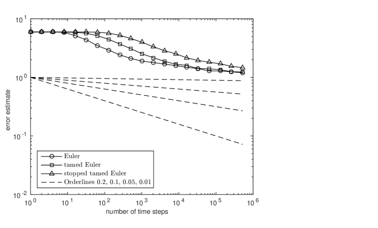
Figure 1. Error vs. number of time steps

References

- [1] Alfonsi, A. Strong order one convergence of a drift implicit Euler scheme: Application to the CIR process. Statistics & Probability Letters 83, 2 (2013), 602–607.
- [2] Berkaoui, A., Bossy, M., and Diop, A. Euler scheme for SDEs with non-Lipschitz diffusion coefficient: strong convergence. ESAIM Probab. Stat. 12 (2008), 1–11 (electronic).
- [3] Beyn, W.-J., Isaak, E., and Kruse, R. Stochastic C-stability and B-consistency of explicit and implicit Euler-type schemes. arXiv:1411.6961 (2014), 29 pages.
- [4] Chassagneux, J.-F., Jacquier, A., and Mihaylov, I. An explicit euler scheme with strong rate of convergence for non-lipschitz sdes. arXiv:1405.3561 (2014), 27 pages.
- [5] Clark, J. M. C., and Cameron, R. J. The maximum rate of convergence of discrete approximations for stochastic differential equations. In Stochastic differential systems (Proc. IFIP-WG 7/1 Working Conf., Vilnius, 1978), vol. 25 of Lecture Notes in Control and Information Sci. Springer, Berlin, 1980, pp. 162–171.
- [6] Dereich, S., Neuenkirch, A., and Szpruch, L. An Euler-type method for the strong approximation of the Cox-Ingersoll-Ross process. Proc. R. Soc. Lond. Ser. A Math. Phys. Eng. Sci. 468, 2140 (2012), 1105–1115.
- [7] Gyöngy, I. A note on Euler’s approximations. Potential Anal. 8, 3 (1998), 205–216.
- [8] Gyöngy, I., and Rásonyi, M. A note on Euler approximations for SDEs with Hölder continuous diffusion coefficients. Stochastic Process. Appl. 121, 10 (2011), 2189–2200.
- [9] Hairer, M., Hutzenthaler, M., and Jentzen, A. Loss of regularity for Kolmogorov equations. Ann. Probab. 43, 2 (2015), 468–527.
- [10] Higham, D. J., Mao, X., and Stuart, A. M. Strong convergence of Euler-type methods for nonlinear stochastic differential equations. SIAM J. Numer. Anal. 40, 3 (2002), 1041–1063 (electronic).
- [11] Hofmann, N., Müller-Gronbach, T., and Ritter, K. The optimal discretization of stochastic differential equations. J. Complexity 17, 1 (2001), 117–153.
- [12] Hu, Y. Semi-implicit Euler-Maruyama scheme for stiff stochastic equations. In Stochastic analysis and related topics, V (Silivri, 1994), vol. 38 of Progr. Probab. Birkhäuser Boston, Boston, MA, 1996, pp. 183–202.
- [13] Hutzenthaler, M., and Jentzen, A. On a perturbation theory and on strong convergence rates for stochastic ordinary and partial differential equations with non-globally monotone coefficients. arXiv:1401.0295 (2014), 41 pages.
- [14] Hutzenthaler, M., Jentzen, A., and Kloeden, P. E. Strong convergence of an explicit numerical method for SDEs with non-globally Lipschitz continuous coefficients. Ann. Appl. Probab. 22, 4 (2012), 1611–1641.
- [15] Hutzenthaler, M., Jentzen, A., and Noll, M. Strong convergence rates and temporal regularity for cox-ingersoll-ross processes and bessel processes with accessible boundaries. arXiv: (2014), 32 pages.
- [16] Hutzenthaler, M., Jentzen, A., and Wang, X. Exponential integrability properties of numerical approximation processes for nonlinear stochastic differential equations. arXiv:1309.7657 (2013), 32 pages.
- [17] Klenke, A. Probability theory. Universitext. Springer-Verlag London Ltd., London, 2008. A comprehensive course, Translated from the 2006 German original.
- [18] Mao, X., and Szpruch, L. Strong convergence rates for backward Euler-Maruyama method for non-linear dissipative-type stochastic differential equations with super-linear diffusion coefficients. Stochastics 85, 1 (2013), 144–171.
- [19] Maruyama, G. Continuous Markov processes and stochastic equations. Rend. Circ. Mat. Palermo (2) 4 (1955), 48–90.
- [20] Müller-Gronbach, T. The optimal uniform approximation of systems of stochastic differential equations. Ann. Appl. Probab. 12, 2 (2002), 664–690.
- [21] Müller-Gronbach, T. Strong approximation of systems of stochastic differential equations. Habilitation thesis, TU Darmstadt (2002), iv+161.
- [22] Müller-Gronbach, T. Optimal pointwise approximation of SDEs based on Brownian motion at discrete points. Ann. Appl. Probab. 14, 4 (2004), 1605–1642.
- [23] Müller-Gronbach, T., and Ritter, K. Minimal errors for strong and weak approximation of stochastic differential equations. In Monte Carlo and quasi-Monte Carlo methods 2006. Springer, Berlin, 2008, pp. 53–82.
- [24] Neuenkirch, A., and Szpruch, L. First order strong approximations of scalar SDEs defined in a domain. Numerische Mathematik (2014), 1–34.
- [25] Rümelin, W. Numerical treatment of stochastic differential equations. SIAM J. Numer. Anal. 19, 3 (1982), 604–613.
- [26] Sabanis, S. Euler approximations with varying coefficients: the case of superlinearly growing diffusion coefficients. arXiv:1308.1796 (2013), 21 pages.
- [27] Sabanis, S. A note on tamed Euler approximations. Electron. Commun. Probab. 18 (2013), 1–10.
- [28] Schurz, H. An axiomatic approach to numerical approximations of stochastic processes. Int. J. Numer. Anal. Model. 3, 4 (2006), 459–480.
- [29] Traub, J. F., Wasilkowski, G., and Woźniakowski, H. Information-based complexity. Boston, MA: Academic Press, Inc., 1988.
- [30] Tretyakov, M., and Zhang, Z. A fundamental mean-square convergence theorem for SDEs with locally Lipschitz coefficients and its applications. SIAM J. Numer. Anal. 51, 6 (2013), 3135–3162.
- [31] Wang, X., and Gan, S. The tamed Milstein method for commutative stochastic differential equations with non-globally Lipschitz continuous coefficients. Journal of Difference Equations and Applications 19, 3 (2013), 466–490.