Influence of the multipole order of the source on the decay of an inertial wave beam in a rotating fluid

Abstract

We analyze theoretically and experimentally the far-field viscous decay of a two-dimensional inertial wave beam emitted by a harmonic line source in a rotating fluid. By identifying the relevant conserved quantities along the wave beam, we show how the beam structure and decay exponent are governed by the multipole order of the source. Two wavemakers are considered experimentally, a pulsating and an oscillating cylinder, aiming to produce a monopole and a dipole source, respectively. The relevant conserved quantity which discriminates between these two sources is the instantaneous flowrate along the wave beam, which is non-zero for the monopole and zero for the dipole. For each source the beam structure and decay exponent, measured using particle image velocimetry, are in good agreement with the predictions.

I Introduction

In rotating fluids, the restoring action of the Coriolis force allows for the propagation of anisotropic, transverse, circularly polarized waves called inertial waves.GreenspanBook These waves are of fundamental interest for geo- and astrophysical flows:Aldridge_Toomre_1969 ; Aldridge_Lumb_1987 ; Suess_1971 they can for instance be excited in the fluid core of planets by tidal motions, precession or libration.Kerswell1995 ; Rieutord2001 ; Kida2011 Internal gravity waves in stratified fluids, relevant to the ocean and the atmosphere, share a number of properties with inertial waves.Lighthill1978 ; Pedlosky1987 Internal waves, or mixed internal–inertial waves when rotation and stratification effects are of comparable magnitude,Peat1978 ; Peacock2005 can also be excited in the ocean by the interaction of tides with topography.Wunsch2004 ; Garrett2007 ; Echeverrri2010 ; Swart2010

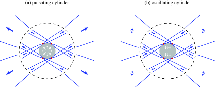
Figure 1: (Color online) Sketch of the far-field wave beams resulting from a combination of parent beams emitted from the critical lines, for (a) a pulsating cylinder and (b) an oscillating cylinder. The size of the disturbance is assumed much larger than the thickness of the Ekman boundary layer. The dashed circles represent the separation between bimodal and unimodal regions. Eight wave beams are emitted from four critical lines (red points), which behave as local sources of non-zero instantaneous flowrate. Far from the cylinder, two parent beams propagating in the same direction combine and form a unique beam. The instantaneous flowrate of the resulting merged beam is non-zero when the two parent beams are in phase (case a), and is zero when they are out of phase (case b).

We focus in this paper on the scaling of the viscous decay of a wave beam emitted by a line source in a uniformly rotating fluid. Although this problem has received much attention, the influence of the multipole order of the source has not been addressed so far. Interestingly, whereas the growth of the wave beam thickness,Walton1975 $\delta(x)\sim x^{1/3}$ (with $x$ the distance from the source), is independent of the multipole order of the source, the decay of the wave amplitude depends on which quantity is conserved along the wave beam (flowrate, momentum, or higher order moment), which is directly governed by the multipole order of the source. Such dependence was discussed in the case of internal waves produced by a point source in stratified fluids by Voisin.Voisin2003 Here we address this problem for a two-dimensional inertial wave beam produced by a line source, extending the simple far-field quasi-parallel approach of Cortet et al.Cortet2010 to a source of arbitrary multipole order. We show that the wave decay is steeper as the multipole order of the source increases, which implies that the far-field decay of a wave beam emitted by an arbitrary source is dominated by its lowest multipole component.

Inertial wave beams emitted from localized sources are relevant to a broad range of laboratory and natural flows, including local forcing by a wavemaker immersed in the fluid, but also global forcing such as precession, libration or tidal motion acting at the scale of the fluid domain. This is because in all cases wave beams are emitted from critical lines, where the local slope of the solid boundaries equals the propagation angle of the wave. Along such critical lines the oscillating boundary layer erupts and forms oscillating beams in the bulk of the flow.GreenspanBook ; Kerswell1995 ; Hollerbach1995 ; Rieutord2001 ; Rieutord2002 ; Calkins2010 In confined fluid domains such beams reflect and, in the presence of sloping boundaries, may focus on wave attractors.Tilgner1999 ; Maas2001 ; Rieutord2001 ; Manders2003 The eruption at critical lines produces two types of wave beams, associated with different magnitudes and scaling laws, propagating in planes tangent and non-tangent to the solid boundary.Kerswell1995 Wave emission in the tangent plane, developing only along convex boundaries, is stronger: this is the case for conical inertial wave beams emitted from the inner core of a rotating spherical shell,Kerswell1995 ; Hollerbach1995 or for internal wave beams excited by oceanic internal tides on the edge of continental shelves or ridges.Wunsch2004 ; Garrett2007 ; Gostiaux2007 ; Echeverrri2010 Wave emission in the non-tangential plane, both at critical lines of convex or concave slope (for instance on the outer sphere of a rotating spherical shellKerswell1995 ; Hollerbach1995 ; Rieutord2001 or at the sloping bottom of a ridgeSwart2010 ), is of weaker amplitude. Emission of inertial wave beams is also observed from horizontal edges in containers such as a cylinderMcEwan1970 ; Duguet2006 or a parallelepiped.Boisson2012b

A key property of an inertial wave beam spawned from an erupting boundary layer is its non-zero instantaneous flowrate: it can be modeled in the far field as originating from a monopole line source. Depending on the topology of the fluid domain, in particular on the distribution and relative phases between such elementary monopole sources, different wave beams propagating in the same direction may combine and form far-field beams of either non-zero or zero instantaneous flowrate, therefore corresponding to an effective monopole or a higher order multipole source. Note that such combination of beams requires propagation over a distance much larger than the separation between the sources, a requirement which is usually not satisfied in geo- and astrophysical situations.

We restrict in the following to wave beams produced by effective line sources surrounded by the fluid. In practical situations, such line source corresponds to a two-dimensional convex disturbance, say a cylinder, defining four critical lines (Fig. 1). If the cylinder is pulsating (Fig. 1a), the periodic emission and suction of mass from these critical lines is in phase, so the far-field merged beams have non-zero flowrate: this defines an effective monopole source. On the other hand, if the cylinder is oscillating (Fig. 1b), the parent beams propagating in the same direction are out of phase, resulting in far-field merged beams of zero flowrate: this defines an effective dipole source. The pulsating and oscillating cylinders are therefore generic configurations to investigate the influence of the multipole order of a line source on the properties of the far-field wave beams.

Most of the experiments investigating wave beams emitted by a local disturbance, both in stratifiedMowbray1967 ; Thomas1972 ; Flynn2003 ; Zhang2007 ; Gostiaux2007 ; Voisin2011 and rotatingMessio2008 ; Cortet2010 fluids, are based on oscillating wavemakers (with the exception of Makarov et al.Makarov1990 who report results from a pulsating cylinder in a stratified fluid). The resulting far-field wave beams are therefore distinct from those produced from an erupting boundary layer in a globally forced fluid domain. The aim of the present paper is to compare the far-field properties of inertial wave beams emitted from a pulsating and an oscillating cylinder in a rotating tank, aiming to produce a monopole and a dipole source. Velocity measurements in the wave beam are achieved using two-camera multi-resolution particle image velocimetry, ensuring a good resolution both in the near and far fields. The two sources produce distinct decay exponents and wave beam profiles, in good agreement with the theoretical predictions.

II Theoretical background

II.1 Dispersion relation and viscous spreading

The geometrical properties of inertial waves follow from their dispersion relation,GreenspanBook

$$\sigma=\pm\frac{2\mathbf{\Omega}\cdot\mathbf{k}}{|\mathbf{k}|}=2\Omega\cos\theta,$$ (1)

with $\sigma>0$ the wave frequency and $\theta$ the polar angle between the wave vector $\mathbf{k}$ and the vertical rotation vector $\mathbf{\Omega}$. Waves emitted from a localized harmonic disturbance propagate energy in directions making an angle $\pm\theta$ to the horizontal, along two cones for a point source and along four plane beams for a line source normal to $\mathbf{\Omega}$. We restrict in the following to the line source configuration, for which the spatial decay of the wave is purely governed by viscosity. In each wave beam, fluid particles describe anticyclonic circular translations in the tilted plane normal to $\mathbf{k}$. Since only the orientation of $\mathbf{k}$ is prescribed by the dispersion relation (1) but not its magnitude, the characteristic sizes of the wave (wave length, beam thickness) are governed by the boundary conditions and viscosity.

The viscous spreading of the wave beam results from the combination of the energy propagation in the longitudinal direction $x$ and its diffusion in the lateral direction $z$ (see Fig. 2). Its scaling can be obtained from a classical boundary-layer argument: During a time $t$, the wave energy spreads laterally over a distance $\delta\simeq\sqrt{\nu t}$, with $\nu$ is the kinematic viscosity, and propagates over a distance $x=c_{g}t$, where $c_{g}$ is the group velocity. Evaluating $c_{g}=(\sigma/k)\tan\theta$ for the dominant wave number at a distance $x$ from the source, $k\sim\delta^{-1}$, simply yields

$$\delta(x)\sim\ell^{2/3}x^{1/3},$$ (2)

where we introduce the viscous scale

$$\ell=(\nu/\sigma\tan\theta)^{1/2}.$$ (3)

Although the scaling of the wave amplitude strongly depends on the multipole order of the source, the scaling of the beam thickness (2) is independent of the nature of the source, provided that $\delta(x)$ is much larger than the size of the source.

II.2 Boundary layer equations

We derive now the similarity solutions for a viscous 2D inertial wave beam emitted by a harmonic line source, focusing on the spatial decay of the wave amplitude and its dependence on the multipole order of the source. The derivation follows that of Thomas and StevensonThomas1972 for internal waves in stratified fluids. We use the velocity–vorticity formulation of Cortet et al.,Cortet2010 generalized here to a source of arbitrary order.

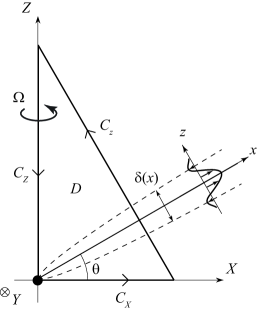
Figure 2: Two-dimensional wave beam emitted from a line source at $(X=0,Z=0)$ in a fluid rotating about the $Z$ axis. Only the beam propagating in the first quadrant ($X>0$, $Z>0$) is shown. The contour $C$ shows the frontiers of the domain of integration $D$ used in Sec. II.3.

We consider a line source along the $Y$ axis, of angular frequency $\sigma$, in a fluid rotating at rate $\Omega$ about the $Z$ axis (Fig. 2). The four wave beams emitted by the source being invariant along $Y$, energy propagates in the $(X,Z)$ plane. In the following, we consider only the wave beam propagating in one given quadrant. We start from the linearized vorticity equation in the rotating frame

$$\partial_{t}\bm{\omega}=(2\mathbf{\Omega}\cdot\nabla)\mathbf{u}+\nu\nabla^{2}\bm{\omega},$$ (4)

with $\mathbf{u}$ the velocity and $\bm{\omega}=\nabla\times\mathbf{u}$ the vorticity. We project (4) on the local frame of the far-field wave beam, $(\mathbf{e}_{x},\mathbf{e}_{y},\mathbf{e}_{z})$, with $\mathbf{e}_{x}$ aligned with the group velocity, making angle $\theta=\cos^{-1}(\sigma/2\Omega)$ with the horizontal, and assume that the flow inside the wave beam is quasi-parallel (boundary layer approximation), i.e., such that $|u_{x}|,|u_{y}|\gg|u_{z}|$; $|\omega_{x}|,|\omega_{y}|\gg|\omega_{z}|$ and $\nabla^{2}\simeq\partial_{z}^{2}$. We introduce the complex velocity and vorticity fields in the tilted plane $(x,y)$, $U=u_{x}+iu_{y}$ and $W=\omega_{x}+i\omega_{y}\simeq i\partial_{z}U$. Searching for harmonic solutions of the form $U=U_{0}e^{-i\sigma t}$, Eq. (4) writes

$$\partial_{x}U_{0}+i\ell^{2}\partial_{z}^{3}U_{0}=0.$$ (5)

This equation admits similarity solutions as a function of the reduced transverse coordinate $\eta=z/(x^{1/3}\ell^{2/3})$ of the form

$$U_{0}(x,z)=\tilde{U}_{0}\left(\frac{\ell}{x}\right)^{a}f(\eta),$$ (6)

where $\tilde{U}_{0}$ is a complex velocity scale and $a>0$ the decay exponent to be determined. The solution considered in Cortet et al.Cortet2010 was derived for the particular case $a=1/3$.footnote Inserting Eq. (6) in Eq. (5) yields

$$3f^{\prime\prime\prime}+i\eta f^{\prime}+3iaf=0.$$ (7)

Solutions of this equation, first given by Moore and SaffmanMoore1969 for the problem of a vertical steady shear layer ($\theta=\pi/2$), and later by Thomas and StevensonThomas1972 in the context of internal waves, are

$$f_{m}(\eta)=c_{m}(\eta)+is_{m}(\eta)=\int_{0}^{\infty}K^{m}e^{-K^{3}}e^{iK\eta}dK,$$ (8)

with $c_{m}$ and $s_{m}$ real functions, even and odd respectively. The properties of these functions were considered in detail by Voisin.Voisin2003 Integrating Eq. (8) by parts gives $3f_{m+3}-i\eta f_{m+1}-(m+1)f_{m}=0$ for $m>-1$, which (using $f^{\prime}_{m}=if_{m+1}$) yields

$$3f^{\prime\prime\prime}_{m}+i\eta f^{\prime}_{m}+i(m+1)f_{m}=0.$$ (9)

Comparing with Eq. (7) allows us to relate the decay exponent $a$ of the velocity amplitude to the order $m$ of the Moore-Saffman function,

$$a=\frac{m+1}{3}.$$ (10)

Any localized wave motion can be represented as a sum of Moore–Saffman functions of different orders $m$, each leading to a wave component characterized by a distinct decay exponent (10). This decay exponent agrees with the derivation of PeatPeat1978 for $m=1$, and with the case $m=0$ discussed by Rieutord et al.Rieutord2001 in the problem of detached layers from critical latitudes in a rotating spherical shell. Equation (10) is also consistent with the derivation of VoisinVoisin2003 for internal waves in a stratified fluid (the derivation given in this reference is for the conical wavepacket emitted by a point source, yielding a modified decay exponent $a_{axi}=a+2/3$).

For a wave beam of order $m$, we can write explicitly the velocity component along the wave beam $u_{x}=\Re(U)$ as

$$u_{x}^{(m)}(x,\eta,t)=|\tilde{U}_{0}|\left(\frac{\ell}{x}\right)^{(m+1)/3}(c_{m}(\eta)\cos(\sigma t+\alpha)+s_{m}(\eta)\sin(\sigma t+\alpha)),$$ (11)

and the vorticity component $\omega_{y}=\Im(W)$ as

$$\omega_{y}^{(m)}(x,\eta,t)=\frac{|\tilde{U}_{0}|}{\ell}\left(\frac{\ell}{x}\right)^{(m+2)/3}(-s_{m+1}(\eta)\cos(\sigma t+\alpha)+c_{m+1}(\eta)\sin(\sigma t+\alpha)),$$ (12)

where $\tilde{U}_{0}=|\tilde{U}_{0}|e^{-i\alpha}$. The argument $\alpha$ accounts for a possible phase shift, through added mass effects, between the wave beam oscillation and the source oscillation. These quantities (11) and (12) are of interest for the experimental measurements based on two-component particle imaging velocimetry in the $(X,Z)$ plane described in Sec. III.

II.3 Conservation laws

We demonstrate now that the order $m$ of the Moore–Saffman function describing a wave beam in the far field coincides with the multipole order $n$ of the source from which it is emitted. We define in the following a source of order $n$ such that the moments of order $s$ of the rate of expansion $\mu(X,Z,t)=\nabla\cdot\mathbf{u}$ are zero for $s<n$ and finite for $s=n$. We note first that the moment of order $s$ of the Moore-Saffman function $f_{m}(\eta)$ (8) satisfies the property

$$\int_{-\infty}^{\infty}\eta^{s}f_{m}(\eta)\,d\eta=\begin{cases}0&\text{($s<m$)},\\ i^{s}\pi s!&\text{($s=m$)},\\ \infty&\text{($s>m$)},\end{cases}$$ (13)

so that only the $m$-th moment of the velocity profile of order $m$ (11) is finite and non-zero. What is needed in addition is to find a conserved quantity involving that moment, and to identify $m$ to the multipole order of the source from which the wave beam is emitted.

Consider first a line monopole ($n=0$) along the $Y$-axis, releasing fluid at the flowrate $q(t)$ per unit length. The corresponding rate of expansion $\mu(X,Z,t)$ has $q(t)$ as its zeroth moment,

$$q(t)=\int\mu(X,Z,t)\,dXdZ,$$ (14)

and is of the form

$$\mu(X,Z,t)=q(t)\delta(X)\delta(Z),$$ (15)

with $\delta$ the Dirac delta function. For a domain $D$ of boundary $C$ in the $(X,Z)$-plane, we have, by the divergence theorem,

$$\oint_{C}\mathbf{u}\cdot\mathbf{n}\,dl=\int_{D}\mu\,dXdZ,$$ (16)

where $\mathbf{n}$ is the outward normal and $dl$ a positively oriented contour element. We specialize to the first quadrant and consider the domain represented in Fig. 2; its boundary starts from the origin along a segment $C_{X}$ of the $X$-axis, continues with a segment $C_{z}$ perpendicular to the wave beam at a large distance $x$, and goes back to the origin along a segment $C_{Z}$ of the $Z$-axis. The contributions of $C_{X}$ and $C_{Z}$ to the contour integral vanish, since the velocity is negligible outside the beam. The surface integral is one fourth of the integral over the whole plane, owing to the parity of the delta function. We eventually obtain

$$\int_{-\infty}^{\infty}u_{x}\,dz=\tfrac{1}{4}q(t),$$ (17)

a conservation equation of the type used by Moore and SaffmanMoore1969 and Rieutord et al.,Rieutord2001 involving the zeroth moment of the longitudinal velocity.

Consider next a line dipole ($n=1$), defined such that the flowrate (zeroth moment of the rate of expansion $\mu$) is zero, but the first moment

$$\mathbf{p}(t)=\int\mathbf{x}\,\mu(X,Z,t)\,dXdZ,$$ (18)

is finite: it is related to the momentum per unit length imparted to the fluid. The rate of expansion $\mu$ therefore writes

$$\mu(X,Z,t)=-\mathbf{p}(t)\cdot\nabla(\delta(X)\delta(Z)),$$ (19)

as discussed for example by Pierce.Pierce1989 We write, with $x_{i}$ an arbitrary coordinate in the plane $(X,Z)$ and $u_{i}$ the associated velocity component,

$$\nabla\cdot(x_{i}\mathbf{u})=x_{i}(\nabla\cdot\mathbf{u})+u_{i}.$$ (20)

Integration over an arbitrary domain $D$ yields

$$\oint_{C}x_{i}\mathbf{u}\cdot\mathbf{n}\,dl=\int_{D}x_{i}\mu\,dXdZ+\int_{D}u_{i}\,dXdZ,$$ (21)

which becomes, after application to the domain $D$ of Fig. 2,

$$\int_{-\infty}^{\infty}x_{i}u_{x}\,dz=\tfrac{1}{4}p_{i}+\int_{0}^{\infty}\!\!\!\int_{0}^{\infty}u_{i}\,dXdZ.$$ (22)

We finally choose $x_{i}=z$, the cross-beam coordinate, such that $u_{i}=u_{z}$ is negligible everywhere in the quadrant. The last integral vanishes in Eq. (22) and we obtain

$$\int_{-\infty}^{\infty}zu_{x}\,dz=\tfrac{1}{4}p_{z}(t),$$ (23)

a conservation equation involving the first moment of the longitudinal velocity. This equation is equivalent to those used by Thomas and StevensonThomas1972 and Peat,Peat1978 involving the zeroth moments of the pressure and stream function, respectively. We conclude that the velocity profile in a wave beam emitted by a line dipole ($n=1$) has a vanishing moment of order $s=0$ (17) and a finite moment of order $s=1$ (23).

The previous argument can be generalized to a line source of arbitrary multipole order: the wave beam emitted from a source of order $n$ is such that the $s$-th moment of the longitudinal velocity is zero for $s<n$ and finite for $s=n$. This finite moment writes (see Appendix A)

$$\int_{-\infty}^{\infty}z^{n}u_{x}\,dz=\tfrac{1}{4}q_{z\cdots z}(t),$$ (24)

with $q_{z\cdots z}$ the $n$-th moment of the rate of expansion $\mu(X,Z,t)$ along the $z$ axis. Switching to complex notation, $u_{x}^{(m)}=\Re(U_{0}e^{-i\sigma t})$ and $q_{z\cdots z}=\Re(Q_{z\cdots z}e^{-i\sigma t})$, and using Eq. (6) yield

$$\tilde{U}_{0}\ell^{1+n}\left(\frac{\ell}{x}\right)^{(m-n)/3}\int_{-\infty}^{\infty}\eta^{n}f_{m}(\eta)\,d\eta=\tfrac{1}{4}Q_{z\cdots z}.$$ (25)

Using the property (13) of $f_{m}(\eta)$ yields immediately $m=n$ and

$$\tilde{U}_{0}=\frac{(-i)^{n}}{n!}\frac{Q_{z\cdots z}}{4\pi\ell^{n+1}},$$ (26)

confirming that the order $m$ of the Moore–Saffman wave beam is equal to the multipole order $n$ of the source from which it is emitted.

We can conclude that a beam emitted by a monopole source is essentially an oscillating jet of non-zero instantaneous flowrate. On the other hand, a wave beam emitted by a multipolar source of order $m>0$ contains a set of oscillating shear layers with zero instantaneous flowrate, the number of layers in the beam increasing as $m^{1/3}$ for large $m$. The stronger shear stress induced by the larger number of layers naturally results in a steeper decay of the wave amplitude.

For a source of arbitrary shape, characterized by an arbitrary multipole expansion, the viscous decay of the wave beams in the far-field is dominated by the smallest decay exponent $a$, i.e. by the term of lowest order in the expansion. In practice we can focus on the first two orders: monopole ($m=0$) for any source of finite flowrate, for which $u_{x}\sim x^{-1/3}$ and $\omega_{y}\sim x^{-2/3}$, and dipole ($m=1$) for a source of zero flowrate, for which $u_{x}\sim x^{-2/3}$ and $\omega_{y}\sim x^{-1}$.

III Experimental setup and data analysis

We have set up an experiment to characterize the influence of the multipole order of the source on the structure and decay of the inertial wave beam. Measurements are performed in a tank of horizontal size $L_{X}\times L_{Y}=150\times 80$ cm², filled with 50 cm of water, and mounted on a 2 m diameter platform rotating around the vertical axis $Z$. Two wavemakers are considered, referred to as pulsating source and oscillating source [see Fig. 3(a,b)]. These wavemakers aim to produce effective monopole and dipole sources (properties summarized in Tab. 1):

• The pulsating source consists in a water-filled horizontal rubber tube, 60 cm long, whose volume varies as $\sin(\sigma t)$. The instantaneous radius varies approximately as $R(t)\simeq R_{0}+A\sin(\sigma t)$, with mean radius $R_{0}=8.9$ mm and amplitude $A=0.7$ mm (the oscillation is harmonic to within $A/R_{0}\simeq 8$%). This source imposes an oscillating flow rate per unit length $q(t)\simeq 2\pi R_{0}A\sigma\cos(\sigma t)$.

• The oscillating source consists in a horizontal cylinder, 60 cm long, $R_{0}=3.0$ mm in radius, whose vertical position $Z(t)=Z_{0}+A\sin(\sigma t)$ oscillates at frequency $\sigma$ and amplitude $A=3.2$ mm (Fig. 3(b)). This cylinder is a source of zero net flowrate which can be modeled, at large distances, as an oscillating dipole characterized by a dipole moment $\mathbf{p}(t)=\Re(\mathbf{P}e^{-i\sigma t})$, with $\mathbf{P}=[1+C(\sigma)]\pi R_{0}^{2}A\sigma\mathbf{e}_{Z}$ and $C(\sigma)$ an added mass coefficient. Without background rotation, this coefficient is a real constant $C=1$. With rotation, the coefficient becomes complex and frequency-dependent owing to wave generation. The experimental measurement and theoretical determination of added mass coefficients have been considered by Ermanyuk and GavrilovErmanyuk2002a and Ermanyuk,Ermanyuk2002b among others, for internal waves.

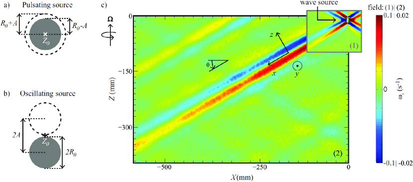
Figure 3: (Color online) Schematic cross-section of the pulsating (a) and oscillating (b) sources (the two extreme states of the oscillation are shown). (c) Vorticity component $\omega_{y}$ showing the wave beam emitted by the oscillating source, measured by the two cameras with different resolutions ($\Omega=0.68$ rad s^-1, propagation angle $\theta=\cos^{-1}(\sigma/2\Omega)\simeq 30$°). Different color scales are used for the two fields for better visibility.

Source	$R_{0}$	$A$	$A\sigma$	$Re$	Vorticity decay exponent
	[mm]	[mm]	[mm s-1]		Theory	Experiment
Pulsating ($m=0$)	8.9	0.7	0.82	15	$-2/3$	$-0.64\pm 0.09$
Oscillating ($m=1$)	3.0	3.2	3.77	23	$-1$	$-0.99\pm 0.05$

Table 1: Properties of the pulsating and oscillating sources: mean radius $R_{0}$, oscillation amplitude $A$, velocity amplitude $A\sigma$, Reynolds number $Re=2R_{0}A\sigma/\nu$ (with $\nu=10^{-6}$ m² s^-1 the kinematic viscosity of water). The vorticity decay exponents correspond to the average ($\pm$ standard deviation) over the four experiments at different $\sigma/2\Omega$ [see Fig. 4(b)].

The wavemaker (either pulsating or oscillating) is immersed horizontally 10 cm below the surface. It is located along the $Y$ axis, at a distance $\Delta X=30$ cm from the side wall of the tank. The wavemaker frequency is kept constant, $\sigma=1.18$ rad s^-1, so that the wavemaker velocity $A\sigma$ is constant. The rotation rate of the platform $\Omega$ is varied in the range 0.68 to 1.68 rad s^-1 (6.5 to 16 rpm), resulting in a beam angle $\theta=\cos^{-1}(\sigma/2\Omega)$ varying in the range $30-70^{\mathrm{o}}$.

The Reynolds number of the flow in the vicinity of the wavemaker, defined as $Re=2R_{0}A\sigma/\nu$, is $Re=15$ for the pulsating source and $Re=23$ for the oscillating source. Despite the relatively large amplitude ratio (up to $A/R_{0}=1.06$ for the oscillating cylinder), these moderate Reynolds numbers indicate that nonlinearities (saturation and generation of higher harmonics) can be neglected; see in particular the discussion by Voisin et al.Voisin2011 for internal waves, pointing the importance of $(A/R_{0})\mathit{Re}$ for saturation. The viscous scale $\ell$ (3) varies in the range $0.6$–$1.2$ mm. For the pulsating cylinder, the ratio $R_{0}/\ell\simeq 7-14$ indicates that the far-field properties of the wave beams are expected at a significant distance $x/\ell$ (the radius of the oscillating cylinder can be made arbitrarily small, but the radius of the pulsating cylinder is limited by the design of the rubber tube).

The two components of the velocity fields $(u_{X},u_{Z})$ are measured in the vertical plane $Y=L_{Y}/2$ normal to the source axis using a particle image velocimetry (PIV) system mounted in the rotating frame. Among the four wave beams emitted by the sources, we focus on the one propagating over the longest distance, in the bottom-left direction [see Fig. 3(c)]. Images of particles are acquired with two $2360\times 1776$ pixels cameras operating simultaneously with different fields of view. Each PIV acquisition consists in 3 000 image pairs (one image per camera) recorded at 3 Hz, which represents 16 fields per source period. Cross-correlation between successive images produces velocity fields sampled on a grid of $295\times 222$ vectors, with a spatial resolution of 0.58 mm for the closer view and 2.04 mm for the larger view. The combination of the PIV data from the two cameras allows us to resolve accurately the spatial scales of the wave field for distances from the source $x$ between 10 mm and 1 m.

Two post-processing steps are applied to the PIV fields. First, the velocity time series are phase-averaged at the forcing frequency $\sigma$ in order to filter out contributions from unwanted residual flows. These residual flows originate from thermal convection effects (velocities of the order of 1 mm s^-1), at very small frequencies, and motions due to the precession of the rotating platform induced by the Earth rotationBoisson2012a ($\simeq 0.5$ mm s^-1), at frequency $\Omega$. Second, we apply a spatial Fourier filter to remove flow structures associated to wave vectors $\mathbf{k}$ such that $k_{X}\,k_{Z}>0$. This procedure is useful to remove secondary wave beams reflecting on the tank walls, which intersect the primary beam characterized by $k_{X}\,k_{Z}<0$ and induce spatial oscillations of the wave envelope [see Fig. 3(c)].

Finally, we remap the velocity fields in the tilted frame $(x,z)$ of the beam, with $x$ the distance from the source, making the angle $\theta=\cos^{-1}(\sigma/2\Omega)$ to the horizontal, and compute the out-of-plane vorticity component $\omega_{y}$. A standard second-order finite difference scheme is used to compute $\omega_{y}$, which is comfortably resolved by our twin PIV measurements ensuring at least 40 grid points per wavelength at all distance $x$ from the source. The vorticity and velocity envelopes of the wave field are finally computed as $\omega_{0}(x,z)=\langle 2\omega_{y}^{2}\rangle^{1/2}$ and $u_{0}(x,z)=\langle 2u_{x}^{2}\rangle^{1/2}$, with $\langle\rangle$ a temporal average.

IV Results

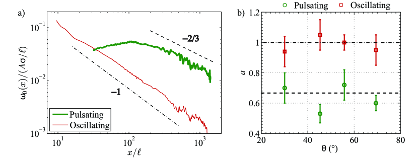
Figure 4: (Color online) (a) Vorticity envelope $\omega_{0}(x,z=0)$ along the direction of the wave beam for the pulsating (thick line) and oscillating (thin line) sources ($\Omega=1.05$ rad s^-1, $\theta\simeq 56$°, $\ell=0.76$ mm). The lines show power laws of exponents $-2/3$ and $-1$ expected theoretically for a monopole and a dipole source respectively. (b) Vorticity decay exponent as a function of the propagation angle $\theta=\cos^{-1}(\sigma/2\Omega)$: (), pulsating source; ($\Square$), oscillating source.

We first compare the spatial decay of the vorticity envelope of the wave beam for the pulsating and oscillating sources. Vorticity is used here instead of velocity to compare against the theory (12) because it is less sensitive to residual large scale flows. The centerline vorticity $\omega_{0}(x,z=0)$ is plotted as a function of the distance $x$ from the source in Fig. 4(a) for $\Omega=1.05$ rad s^-1 ($\theta\simeq 56$°). The distance is normalized by the viscous length $\ell$, and vorticity $\omega_{0}$ is normalized by the source velocity $A\sigma$ and $\ell$. For both sources a power law decay of the vorticity is observed far from the source, but with a different exponent: $\omega_{0}\sim x^{-1.00\pm 0.05}$ for the oscillating source, starting close to the source ($x/\ell>10$) and extending over nearly two decades; $\omega_{0}\sim x^{-0.72\pm 0.10}$ for the pulsating source, starting much further from the source ($x/\ell>200$) and hence visible over a limited range of $x$. These exponents are in good agreement with the predictions for a monopole and a dipole source, $x^{-2/3}$ and $x^{-1}$ respectively [see Eq. (12)]. Exponents measured at other values of $\sigma/2\Omega=\cos\theta$, reported in Fig. 4(b), are consistent with these numbers and do not show any trend with $\theta$.

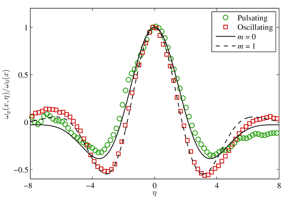
Figure 5: (Color online) Normalized transverse vorticity profiles $\omega_{y}(x,\eta,t)/\omega_{0}(x,0)$ as a function of the reduced transverse coordinate $\eta=z/(x^{1/3}\ell^{2/3})$, compared to the theoretical vorticity profiles $c_{m+1}(\eta)/c_{m+1}(0)$. , pulsating source ($m=0$); $\Square$, oscillating source ($m=1$). The profiles are measured at a distance $x/\ell=330$ from the source, in the region where both beams show a power law decay, and are shown for the time at which the vorticity is maximum at the center of the beam.

Another distinctive property of a wave beam emitted by a monopole or a dipole disturbance is the transverse vorticity profile, given by the function $f_{1}(\eta)$ or $f_{2}(\eta)$ respectively. Figure 5 shows the normalized vorticity profile $\omega_{y}(x,z,t)/\omega_{0}(x,z=0)$ for both sources as a function of the reduced transverse coordinate $\eta=z/(x^{1/3}\ell^{2/3})$, at the time at which $\omega_{y}$ is maximum at the centerline. The normalized profiles, shown here for a distance $x/\ell=330$, are independent of $x$ provided that $x$ is large enough, i.e. in the region showing a well-defined power-law decay ($x/\ell>200$ for the pulsating source and $x/\ell>10$ for the oscillating source). We compare these profiles against the Moore–Saffman functions taken at the same phase, $\omega_{y}(x,\eta,t)/\omega_{0}(x,\eta=0)=c_{m+1}(\eta)/c_{m+1}(0)$, for $m=0$ and $m=1$. The agreement is excellent for both sources, for $|\eta|$ up to $5$, clearly confirming that the order of the Moore–Saffman function that best describes the wave envelope is governed by the multipole order of the source. At larger distance from the beam centerline ($|\eta|>5$), the discrepancy between the theoretical and experimental profiles probably originates from residual fluid motions associated to reflected wave beams that cannot be eliminated by the Fourier filtering procedure.

The flowrate across the wave beam provides another confirmation of the match between the wave beam order and the source multipole order. We compute the flowrate $q(t)$ per unit length by integration over $\eta$ of the instantaneous velocity $u_{x}(x,\eta)$, using a truncation at $|\eta|=6$ to reduce disturbance from fluid motions out of the primary beam of interest. The theoretical flowrate amplitude for each wave beam is $q_{th}=\pi\ell^{2/3}x^{1/3}u_{0}(x,\eta=0)$ for the monopole source and zero for the dipole source. We find a normalized flowrate $q/q_{th}\simeq 1.0\pm 0.05$ for the pulsating cylinder, and $0.07\pm 0.05$ for the oscillating cylinder (the non-zero value in the latter case originates from the truncation of the integral). This normalized flowrate does not depend significantly on the distance from the source in the far-field for both disturbances (to within $\pm 0.05$).

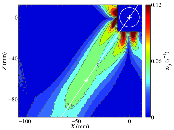
Figure 6: (Color online) Contour plot of the vorticity envelope $\omega_{0}$ from the close-view camera for the pulsating source at $\theta=56^{\mathrm{o}}$, showing the transition from a bimodal to a unimodal wave beam. The white circle shows the source and the white line the far-field wave beam axis. The star marker indicates the location $x_{c}/\ell=110$ at which $\omega_{0}(x)$ is maximum in Fig. 4(a).

We finally turn to the description of the distance $x$ beyond which the scaling law holds for the far-field decay of the wave amplitude. Figure 4(a) shows that the vorticity amplitude decreases at all $x$ for the oscillating source, with a well-defined power law beyond $x/\ell\simeq 10$, while it is non-monotonic for the monopole source with a maximum at $x_{c}/\ell\simeq 110\pm 10$. This non-monotonic profile originates from the transition from a bimodal beam close to the source to a unimodal beam far from the source, as illustrated by the close-up view in Fig. 6. Because of the large extent of the pulsating cylinder compared to the viscous length, the wave field close to the source corresponds to two separate beams propagating in the same direction $\theta=\cos^{-1}(\sigma/2\Omega)$, with a shift of $z=\pm R_{0}=\pm 8.9$ mm from the axis of the far-field beam. Close to the source, the transverse profile is therefore bimodal, with a local minimum at $z=0$, while it becomes unimodal for large distances with a maximum at $z=0$, with a transition occurring around $x_{c}$.

This bimodal-to-unimodal transition, a classical feature of waves emitted from a source of large extent, has been mainly described for internal waves excited by oscillating disturbances.Makarov1990 ; Hurley_Keady_97_2 ; Flynn2003 ; Zhang2007 ; Gostiaux_thesis ; Voisin2011 Figure 1(a,b) provides a simple sketch of this transition for a pulsating and an oscillating cylinder of large extent. The oscillating boundary layer over the cylinder detaches at the four critical lines, where the local slope equals the wave beam angle $\theta$, forming eight wave beams of non-zero instantaneous flowrate. The far-field beam in a given direction results from the merging of two parent beams propagating along the same direction, that are in phase for the pulsating cylinder and out-of-phase for the oscillating cylinder. The combination of two in-phase parent beams of order $m$ separated by a normalized transverse distance $\eta_{0}$ is given by $f_{m}(\eta+\eta_{0}/2)+f_{m}(\eta-\eta_{0}/2)$, which far from the source ($\eta_{0}\ll 1$) simply gives a beam of order $m$. On the other hand, the combination of two out-of-phase parent beams of order $m$ is given by $f_{m}(\eta+\eta_{0}/2)-f_{m}(\eta-\eta_{0}/2)\simeq\eta_{0}f^{\prime}_{m}(\eta)=i\eta_{0}f_{m+1}(\eta)$, yielding a beam of order $m+1$: this is consistent with the observation of a far-field wave beam of zero flowrate ($m=1$) emitted from the two nonzero flowrate sources ($m=0$) at the critical lines for the oscillating cylinder.

Determining the merging distance $x_{c}$ requires the full resolution of the flow close to the wavemaker. This computation is given in Hurley and KeadyHurley_Keady_97_2 and VoisinVoisin2011 for oscillating cylinders and spheres in a stratified fluid. Qualitatively, we can estimate $x_{c}$ from the spreading law $\delta(x)\sim\ell^{2/3}x^{1/3}$ of each parent beam, yielding a merging distance $x_{c}$ such that $\delta(x_{c})\simeq 2R_{0}$ given by $x_{c}/\ell\sim(R_{0}/\ell)^{3}$. The radius ratio between the pulsating and oscillating cylinders ($R_{0}=8.9$ and $3.0$ mm, respectively) indicates that $x_{c}/\ell$ is expected much larger for the pulsating cylinder. For the oscillating cylinder the predicted merging distance is of order of the cylinder radius, so that the bimodal wave beam cannot be observed, which is consistent with the monotonic decay of $\omega_{0}(x)$.

V Conclusion

In this paper we analyzed the decay of a two-dimensional inertial wave beam and showed that it is set by the multipole order $n$ of the source from which it is emitted. Experimental measurements are reported for sources of the first two orders: monopole ($n=0$) and dipole ($n=1$). We find that the structure of the wave beam is well represented by a Moore-SaffmanMoore1969 (or Thomas-StevensonThomas1972 ) function of order equal to the multipole order of the source. The wave envelope decays as a power law of the distance from the source, with an exponent governed by the order of the source ($x^{-(n+1)/3}$ for the velocity and $x^{-(n+2)/3}$ for the vorticity). These properties, demonstrated here for inertial waves in rotating fluids, should also hold for internal waves in stratified fluids.

The steeper decay of the wave amplitude as the multipole order is increased indicates that the far-field structure of a wave beam is dominated by the lowest order of the source, i.e. by its first nonzero moment (flowrate, momentum or higher order moment). In most practical situations, the nature of the source can be discriminated by its instantaneous flowrate, either nonzero for a monopole source or zero for a dipole or higher order source. This means that a wave beam emitted from any source of nonzero instantaneous flowrate must be dominated in the far field by its monopole component. Such monopole sources are relevant to most natural flows (e.g. conical wave beams in the fluid core of planets, internal tide generation over ocean topography): the detachment of the oscillating boundary layers at the critical lines produces oscillating jets in the bulk, corresponding to a weak spatial decay. On the other hand, oscillating disturbances immersed in the fluid (a typical configuration of most laboratory experiments in rotating or stratified fluids) produce in the far field beams of zero instantaneous flowrate, resulting in a stronger spatial decay.

Appendix A Conservation laws for arbitrary multipole order

Equations (17) and (23) relate the zeroth and first moments of the longitudinal velocity to the flowrate and momentum of monopole ($n=0$) and dipole ($n=1$) sources. In this appendix we generalize these relations to sources of arbitrary multipole order $n$. We introduce arbitrary orthogonal coordinates $(x_{1},x_{2})$ in the plane $(X,Z)$, with $(u_{1},u_{2})$ the associated velocity components. The rate of expansion $\mu(X,Z,t)$ of a source of multipole order $n$ has zero moments of order $0$ to $n-1$ and finite $n$-th moments given by

$$q_{i_{1}\cdots i_{n}}(t)=\int x_{i_{1}}\cdots x_{i_{n}}\mu(X,Z,t)\,dXdZ.$$ (27)

These $n$-th moments are tensors of rank $n$ composed of $n+1$ independent scalars. The rate of expansion is of the form

$$\mu(X,Z,t)=\frac{(-1)^{n}}{n!}\sum_{i_{1}=1}^{2}\cdots\sum_{i_{n}=1}^{2}q_{i_{1}\cdots i_{n}}(t)\frac{\partial^{n}}{\partial x_{i_{1}}\cdots\partial x_{i_{n}}}\delta(X)\delta(Z).$$ (28)

Using the identity

$$\nabla\cdot(x_{i_{1}}\cdots x_{i_{n}}\mathbf{u})=x_{i_{1}}\cdots x_{i_{n}}(\nabla\cdot\mathbf{u})+u_{i_{1}}x_{i_{2}}\cdots x_{i_{n}}+\cdots+x_{i_{1}}\cdots x_{i_{n-1}}u_{i_{n}},$$ (29)

and integrating over the domain $D$ of Fig. 2 yield

$$\int_{-\infty}^{\infty}x_{i_{1}}\cdots x_{i_{n}}u_{x}\,dz=\tfrac{1}{4}q_{i_{1}\cdots i_{n}}\\ \mbox{}+\int_{0}^{\infty}\!\!\!\int_{0}^{\infty}(u_{i_{1}}x_{i_{2}}\cdots x_{i_{n}}+\cdots+x_{i_{1}}\cdots x_{i_{n-1}}u_{i_{n}})\,dXdZ.$$ (30)

We choose $(x_{1},x_{2})=(x,z)$ and $i_{1}=\cdots=i_{n}=2$, so that $x_{i_{1}}=\cdots=x_{i_{n}}=z$. The corresponding transverse velocity $u_{i_{1}}=\cdots=u_{i_{n}}=u_{z}$ is negligible, so the last integral vanishes in Eq. (30). We finally obtain Eq. (24), which generalizes Eqs. (17) and (23) to arbitrary multipole order $n$.

References

- (1) H. Greenspan, The Theory of Rotating Fluids (Cambridge University Press, Cambridge, UK, 1968).
- (2) K. D. Aldridge and A. Toomre, “Axisymmetric inertial oscillations of a fluid in a rotating spherical container,” J. Fluid Mech. 37, 307–323 (1969).
- (3) S. T. Suess, “Viscous flow in a deformable rotating container,” J. Fluid Mech. 45, 189–201 (1971).
- (4) K. D. Aldridge and L. I. Lumb, “Inertial waves identified in the Earth’s fluid outer core,” Nature 325, 421–423 (1987).
- (5) R. R. Kerswell, “On the internal shear layers spawned by the critical regions in oscillatory Ekman boundary layers,” J. Fluid Mech. 298, 311–325 (1995).
- (6) S. Kida, “Steady flow in a rapidly rotating sphere with weak precession,” J. Fluid Mech. 680, 150–193 (2011).
- (7) M. Rieutord, B. Georgeot, and L. Valdettaro, “Inertial waves in a rotating spherical shell: attractors and asymptotic spectrum,” J. Fluid Mech. 435, 103–144 (2001).
- (8) J. Lighthill, Waves in Fluids (Cambridge University Press, Cambridge, UK, 1978).
- (9) J. Pedlosky, Geophysical Fluid Dynamics (Springer-Verlag, New York, 1987).
- (10) K. S. Peat, “Internal and inertial waves in a viscous rotating stratified fluid,” Appl. Sci. Res. 33, 481–499 (1978).
- (11) T. Peacock and P. Weidman, “The effect of rotation on conical wave beams in a stratified fluid,” Exp. Fluids 39, 32–37 (2005).
- (12) C. Wunsch and R. Ferrari, “Vertical mixing, energy, and the general circulation of the oceans,” Annu. Rev. Fluid Mech. 36, 281–314 (2004).
- (13) C. Garrett and E. Kunze, “Internal tide generation in the deep ocean,” Annu. Rev. Fluid Mech. 39, 57–87 (2007).
- (14) P. Echeverrri and T. Peacock, “Internal tide generation by arbitrary two-dimensional topography,” J. Fluid Mech. 659, 247–266 (2010).
- (15) A. Swart, L.R.M. Maas, U. Harlander and A.M.M. Manders, “Experimental observation of strong mixing due to internal wave focusing over sloping terrain,” Dynamics of Atmospheres and Oceans 50, 16–34 (2010).
- (16) I.C. Walton, “On waves in a thin rotating spherical shell of slightly viscous fluid,” Mathematika 22, 46–59 (1975).
- (17) B. Voisin, “Limit states of internal wave beams,” J. Fluid Mech. 496, 243–293 (2003).
- (18) P.-P. Cortet, C. Lamriben, and F. Moisy, “Viscous spreading of an inertial wave beam in a rotating fluid,” Phys. Fluids 22, 086603 (2010).
- (19) R. Hollerbach and R. R. Kerswell, “Oscillatory internal shear layers in rotating and precessing flows,” J. Fluid Mech. 298, 327–339 (1995).
- (20) M. Rieutord, L. Valdettaro, and B. Georgeot, “Analysis of singular inertial modes in a spherical shell: the slender toroidal shell model,” J. Fluid Mech. 463, 345– (2002).
- (21) M. A. Calkins, J. Noir, J. D. Eldredge, et J. M. Aurnou, “Axisymmetric simulations of libration-driven fluid dynamics in a spherical shell geometry,” Phys. Fluids 22 (8), 086602 (2010).
- (22) A. Tilgner, “Driven inertial oscillations in spherical shells,” Phys. Rev. E 59 (2), 1789 (1999).
- (23) L.R.M. Maas, “Wave focusing and ensuing mean flow due to symmetry breaking in rotating fluids,” J. Fluid Mech. 437, 13–28 (2001).
- (24) A.M.M. Manders and L.R.M. Maas, “Observations of inertial waves in a rectangular basin with one sloping boundary,” J. Fluid Mech. 493, 39–88 (2003).
- (25) L. Gostiaux and T. Dauxois, “Laboratory experiments on the generation of internal tidal beams over steep slopes,” Phys. Fluids 19, 028102 (2007).
- (26) A. D. McEwan, “Inertial oscillations in a rotating fluid cylinder,” J. Fluid Mech. 40, 603-640 (1970).
- (27) Y. Duguet, J. F. Scott, and L. Le Penven, “Oscillatory jets and instabilities in a rotating cylinder,” Phys. Fluids 18, 104104 (2006).
- (28) J. Boisson, C. Lamriben, L. R. M. Maas, P.-P. Cortet, and F. Moisy, “Inertial waves and modes excited by the libration of a rotating cube,” Phys. Fluids 24, 076602 (2012).
- (29) D. E. Mowbray and B. S. H. Rarity, “A theoretical and experimental investigation of the phase configuration of internal waves of small amplitude in a density stratified liquid,” J. Fluid Mech. 28, 1–16 (1967).
- (30) N. H. Thomas and T. N. Stevenson, “A similarity solution for viscous internal waves,” J. Fluid Mech. 54, 495–506 (1972).
- (31) M. R. Flynn, K. Onu, and B. R. Sutherland, “Internal wave excitation by a vertically oscillating sphere,” J. Fluid Mech. 494, 65–93 (2003).
- (32) H. P. Zhang, B. King, and H. L. Swinney, “Experimental study of internal gravity waves generated by supercritical topography,” Phys. Fluids 19, 096602 (2007).
- (33) B. Voisin, E. V. Ermanyuk, and J.-B. Flór, “Internal wave generation by oscillation of a sphere, with application to internal tides,” J. Fluid Mech. 666, 308–357 (2011).
- (34) L. Messio, C. Morize, M. Rabaud, and F. Moisy, “Experimental observation using particle image velocimetry of inertial waves in a rotating fluid,” Exp. Fluids 44, 519–528 (2008).
- (35) S. A. Makarov, V. I. Neklyudov, and Yu. D. Chashechkin, “Spatial structure of two-dimensional monochromatic internal-wave beams in an exponentially stratified liquid,” Izv. Atmos. Ocean. Phys. 26, 548–554 (1990).
- (36) The decay exponent discussed by Cortet et al. Cortet2010 corresponds to the case of a monopole source, although the wavemaker used in that reference (oscillating cylinder) should behave as a dipole source, for which a steeper decay is expected (). Because of the restricted range of distance from the source, the difference between the two exponents could not be discriminated by the data.
- (37) D. W. Moore and P. G. Saffman, “The structure of free vertical shear layers in a rotating fluid and the motion produced by a slowly rising body,” Phil. Trans. R. Soc. Lond. A 264, 597–634 (1969).
- (38) A. D. Pierce, Acoustics. An Introduction to its Physical Principles and Applications, 2nd ed. (Acoustical Society of America, New York, 1989).
- (39) E. V. Ermanyuk and N. V. Gavrilov, “Force on a body in a continuously stratified fluid. Part 1. Circular cylinder,” J. Fluid Mech. 451, 421–443 (2002).
- (40) E. V. Ermanyuk, “The rule of affine similitude for the force coefficients of a body oscillating in a uniformly stratified fluid,” Exp. Fluids 32, 242–251 (2002).
- (41) J. Boisson, D. Cébron, F. Moisy, and P.-P. Cortet, “Earth rotation prevents exact solid-body rotation of fluids in the laboratory,” EPL 98, 59002 (2012).
- (42) D. G. Hurley and G. Keady, “The generation of internal waves by vibrating elliptic cylinders. Part 2. Approximate viscous solution,” J. Fluid Mech. 351, 119–138 (1997).
- (43) L. Gostiaux, Étude expérimentale des ondes de gravité internes en présence de topographie. Émission, propagation, réflexion, PhD dissertation, École Normale Supérieure de Lyon (2006).