The effects of shape and amplitude on the velocity of scrape-off layer filaments

Abstract

A complete model of the dynamics of scrape-off layer filaments will be rather complex, including temperature evolution, three dimensional geometry and finite Larmor radius effects. However, the basic mechanism of $\boldsymbol{E}\times\boldsymbol{B}$ advection due to electrostatic potential driven by the diamagnetic current can be captured in a much simpler model; a complete understanding of the physics in the simpler model will then aid interpretation of more complex simulations, by allowing the new effects to be disentangled. Here we consider such a simple model, which assumes cold ions and isothermal electrons and is reduced to two dimensions. We derive the scaling with width and amplitude of the velocity of isolated scrape-off layer filaments, allowing for arbitrary elliptical cross-sections, where previously only circular cross-sections have been considered analytically. We also put the scaling with amplitude in a new and more satisfactory form. The analytical results are extensively validated with two dimensional simulations and also compared, with reasonable agreement, to three dimensional simulations having minimal variation parallel to the magnetic field.

Filaments are a prominent feature of the scrape-off layer (SOL) of tokamaks, in L-mode and in H-mode both during and between ELMs[1], and in other magnetised plasmas. They provide a significant component of the particle transport[2], especially in the far SOL, and so may have a strong impact on particle fluxes to the first wall and divertor. Data from gas-puff imaging diagnostics[3] suggests that filaments may sometimes have significantly elliptical (rather than circular) cross-sections. Most of the theoretical work on SOL filaments has been done in simplified, two dimensional models, see [4] and [5] for reviews, but recently there has been an increasing amount of attention given to more realistic models, for example using three dimensional simulations[6, 7, 8] or including finite Larmor radius effects[9]. These developments have motivated us to reexamine and extend the earlier analytical work to try to give as complete a physical picture of the two dimensional mechanisms that regulate filament motion as possible, in order to facilitate the interpretation of more complicated models applied to isolated filaments, and ultimately to SOL turbulence simulations[10, 11, 12].

Our subject here is the scaling of filament velocity with various parameters of the filament, in the two dimensional limit where parallel variation may be neglected and assuming cold ions and isothermal electrons. This represents the very simplest model that can capture the basic mechanism of filament motion. By characterising quantitatively the basic physical processes driving filament motion in this simple model, we will be able, when analysing more complicated models, to identify the deviations from this behaviour. These deviations can then be ascribed to the extra physics in, for example, three dimensional or non-isothermal simulations. The aim therefore is to provide a theoretical tool to aid the interpretation of more complicated models, as part of a programme of research building systematically towards models which are both well enough understood to be trusted and also realistic enough to be quantitatively compared to experiment and used predictively for future machines. The particular model we consider contains two mechanisms that limit the filament velocity: inertia and sheath currents. While inertia is universally present, the sheath current (as modelled here) is only relevant on the assumption that parallel resistivity is small so that parallel currents may reach the sheath unimpeded. Where this assumption is invalid, whether due to cold plasma[13] or interaction with neutrals in the divertor or to large magnetic shear near X-points, different mechanisms will come into play; for some examples see [4]. If it is desired to include other effects, as different closures for the two dimensional equations, we hope that the framework of the calculation provided here will make further additions relatively straightforward.

We present here a calculation of the scaling of the maximum filament velocity allowing arbitrary elliptical cross-sections, which have not previously been considered analytically. We also aim to clarify the physical mechanisms while giving more detail than has previously been published. In particular, the scaling with amplitude, though considered in [14] and mentioned briefly in several works[15, 16, 17], has not previously been given a satisfactory analytical treatment; however, [18] has provided a complete description of the amplitude scaling in the inertial regime from simulations, highlighting the importance of not making the Boussinesq approximation. We use two dimensional simulations of isolated filaments both to identify the qualitative features that go into the calculation, which is especially important for the inertial regime as it is strongly non-linear, and also to validate comprehensively the scaling laws obtained.

1 Velocity scaling

1.1 Physical picture

An isolated filament is, under the assumptions here, a density fluctuation comparable to or larger than the background in amplitude, extended along the magnetic field and with a monopolar structure perpendicular to it. The basic mechanism of filament motion is that there is a current source due to the inhomogeneity of the magnetic field which propels the filament, balanced in the simple model considered here by inertia of the surrounding background plasma and by dissipation from currents through the sheath where the magnetic field intersects the wall at the targets. This description is in some respects inspired by the ‘equivalent circuit’ picture[19, 4]. In contrast to the qualitative description in [4], here we consider drifts/currents only in the fluid model, rather than considering the particle drifts. In order to obtain simple expressions for the filament velocity, we reduce the problem to two dimensions by assuming zero variation parallel to the magnetic field and look only for a maximum velocity of the filament. First we sketch the physical picture, before turning to the full calculation in Section 1.2.

Drive

Due to the curvature of the magnetic field, represented by $\boldsymbol{\kappa}=-\hat{\boldsymbol{x}}/R_{C}$ where $R_{C}$ is the radius of curvature, and the change in its magnitude with radius, $\nabla B=-B\hat{\boldsymbol{x}}/R_{C}$, the diamagnetic current $\boldsymbol{J}_{\mathrm{dia}}=B^{-1}\nabla(nT)\times\hat{\boldsymbol{b}}$ ($\hat{\boldsymbol{b}}\equiv\boldsymbol{B}/B$ being the unit vector in the direction of the magnetic field) has a non-zero divergence, as sketched in Figure 1. This divergence gives a current source whose strength is proportional to the pressure gradient in the direction perpendicular to $\boldsymbol{\kappa}$ and $\nabla B$, which we will call $\hat{\boldsymbol{z}}$. In order to maintain quasineutrality, this current must be closed. Depending on the parameters of the filament, this may occur either through the polarisation current (leading to inertial evolution) or the parallel current (giving rise to sheath current dissipation).

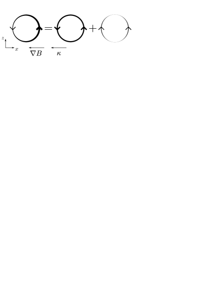
Figure 1: Diamagnetic current in a filament: The width of the line represents the magnitude of the current (integrated in the $\hat{\boldsymbol{b}}$-direction). The diamagnetic current (left) can be split into a divergence-free part (centre) and the remainder (right). This last, divergent part must be closed by parallel or polarisation currents and so provides the drive for filament motion

Inertial evolution

In the absence of dissipation mechanisms (viscosity or sheath currents), there can be no steady state, since the energy of the system increases monotonically[18]. Nevertheless, the filament reaches a maximum velocity, even without dissipation. This contrasts with hydrodynamic drag on a solid object, where the velocity is ultimately limited by viscous dissipation either in a surface layer around the object or in the wake behind it. The mechanism causing the filament velocity to saturate is that it expands as it moves, drawing in fluid from the ‘background’ flow. This is rather like a rocket engine in reverse; instead of generating thrust by expelling material, the filament resists acceleration by absorbing material. The maximum velocity occurs when the rate at which momentum is acquired through this absorption balances the $\boldsymbol{J}\times\boldsymbol{B}$ force from the polarisation current.

Sheath current dissipation

When the current source closes through the parallel current it is regulated by the sheath boundary condition, (12), which determines the current that passes through the Debye sheath to the target plates. For small currents the sheath behaves as an ideal resistor, with current proportional to the electrostatic potential, $\phi$. In steady state the potential is then proportional to the current source, behaving as a simple electrical circuit (Figure 2). The motion of the filament is then just the $\boldsymbol{E}\times\boldsymbol{B}$ drift due to this potential.

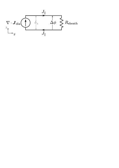
Figure 2: Equivalent circuit for a filament in which the diamagnetic current closes through the parallel current path

1.2 Scaling calculation

We use a coordinate system that takes $\hat{\boldsymbol{x}}$ in the ‘radial’ direction (anti-parallel to the magnetic field curvature and $\nabla B$), $\hat{\boldsymbol{y}}$ along the magnetic field and $\hat{\boldsymbol{z}}$ in the binormal direction. We take the filament to be a monopolar density structure (possibly distorted, in the inertial regime), characterised by two length scales, $\delta_{x}$ and $\delta_{z}$ in the $\hat{\boldsymbol{x}}$- and $\hat{\boldsymbol{z}}$-directions, and an induced, dipolar potential structure. To aid visualisation of the configuration, the density and potential from a simulation (see Section 2) of a filament in the sheath current regime are shown in Figure 3.

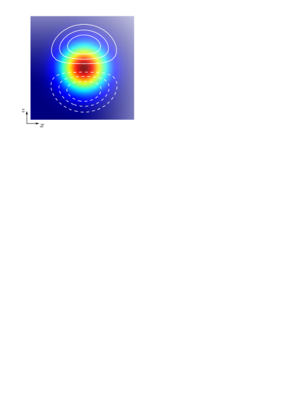
Figure 3: Density (colour-map) and potential (contours; solid for $\phi>0$, dashed for $\phi<0$) for a filament in the sheath regime, at maximum $V_{x}$

We assume cold ions and isothermal electrons, neglect electron inertia and use Bohm normalisation (as in [8], times are normalised to the ion cyclotron frequency $\Omega_{\mathrm{ci}}=eB_{0}/m_{\mathrm{i}}$, lengths to the hybrid Larmor radius $\rho_{\mathrm{s}}=c_{\mathrm{s}}/\Omega_{\mathrm{ci}}$, where $c_{\mathrm{s}}=\sqrt{T_{\mathrm{e}}/m_{\mathrm{i}}}$ is the sound speed, and electrostatic potential by $T_{\mathrm{e}}/e$, with $e$ the elementary charge, $B_{0}$ the magnetic field strength, $m_{\mathrm{i}}$ the ion mass and $T_{e}$ the electron temperature; in addition densities are normalised to a typical value, usually the background density).

The system is driven by the diamagnetic current, and its behaviour determined by whether the divergence of the diamagnetic current closes principally through the polarisation or the parallel current. We now consider each current in turn.

Diamagnetic current

For cold ions, the diamagnetic current is due just to the electron diamagnetic velocity. Neglecting electron inertia and viscosity, the electron momentum equation is

$$0=-\nabla n+n\nabla\phi+n\frac{\boldsymbol{V}_{\mathrm{e}}\times\boldsymbol{B}}{B_{0}}.$$ (1)

Taking the cross product with $\hat{\boldsymbol{b}}$ gives the perpendicular electron velocity with two contributions, the $\boldsymbol{E}\times\boldsymbol{B}$ and diamagnetic velocities: $\boldsymbol{V}_{\mathrm{e}}=\boldsymbol{V}_{E\times B}+\boldsymbol{V}_{\mathrm{dia}}$, with

$$n\boldsymbol{V}_{\mathrm{dia}}=-B_{0}\frac{\nabla n\times\hat{\boldsymbol{b}}}{B}.$$ (2)

Here we must not yet take $B=B_{0}$ ($B_{0}$ being the constant magnetic field used for normalisation) until we have taken its gradient in the divergence of the diamagnetic current:

$$\nabla\cdot\boldsymbol{J}_{\mathrm{dia}} =B_{0}\nabla\cdot\left(\frac{\nabla n\times\hat{\boldsymbol{b}}}{B}\right)$$ (3)

$$=-B_{0}\frac{\nabla n\cdot\nabla\times\hat{\boldsymbol{b}}}{B}-B_{0}\frac{\nabla B\cdot\nabla n\times\hat{\boldsymbol{b}}}{B^{2}}$$

$$=2\frac{\hat{\boldsymbol{z}}\cdot\nabla n}{R_{\mathrm{C}}}=-\hat{\boldsymbol{b}}\cdot\boldsymbol{g}\times\nabla n$$

$$\sim-\frac{g}{\delta_{z}}\left(n-n_{0}\right),$$

for a toroidal magnetic field $\boldsymbol{B}=\boldsymbol{e}_{\phi}/R$ at a major radius $R=R_{\mathrm{C}}$ ($R_{\mathrm{C}}$ denoting the radius of curvature of the magnetic field and $\boldsymbol{e}_{\phi}$ being the unit vector in the toroidal direction) much larger than the size of a filament and defining $\boldsymbol{g}=g\hat{\boldsymbol{x}}=\hat{\boldsymbol{x}}/R_{\mathrm{C}}$.

Polarisation current

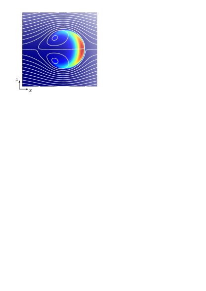
Figure 4: Density (colour-map) and streamlines of flow velocity in the frame of the filament (white) at the time when maximum velocity is reached

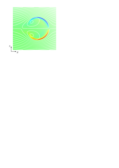
Figure 5: Vorticity (colour-map) and streamlines of flow velocity in the frame of the filament (white) at the time when maximum velocity is reached

Define the filament velocity, $\boldsymbol{V}_{\mathrm{f}}$, as the velocity of the centre of mass of the perturbation,

$$\boldsymbol{V}_{\mathrm{f}}=\int d^{2}x\,(n-n_{0})\boldsymbol{V}$$ (4)

and the ‘filament frame’ as that moving at $\boldsymbol{V}_{\mathrm{f}}$ with respect to the lab frame. In the filament frame there are two distinct regions (see figure 4): the ‘exterior region’ outside the filament where the velocity is always to the left (the streamlines are open); and the ‘filament region’ where the velocity circulates (the streamlines are closed).

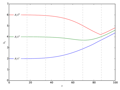
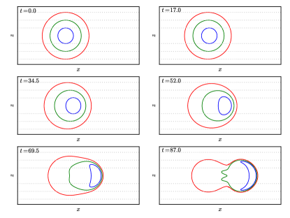
Figure 6: Evolution of three density contours with time. $h_{z}$ is the height of the contour: the difference between the maximum and minimum of $z$ on the contour. The snapshots on the right show the contours (at levels $n=n_{0}\left(1+A/e^{i}\right)$ for $i=1,4,9$ from inside to outside, corresponding to the lines in the left plot) at the times indicated by the dashed vertical lines. $t=87$ is the time at which the filament reaches maximum velocity. The horizontal dotted lines indicate the upper and lower extents of the contours at $t=0$

There is always a force on the filament from the polarisation current $\boldsymbol{J}_{\mathrm{pol}}\times\boldsymbol{b}$ force, which tends to increase its momentum (in the $x$-direction). For the velocity to be constant this gain in momentum must be balanced. In the frame of the background plasma, the balance is provided by absorbing stationary background plasma, which increases the mass of the filament (without adding extra momentum), allowing the velocity to remain constant. Alternatively, considered in the frame of the filament, the background plasma has negative $x$-momentum relative to the filament, providing a loss of momentum to balance the gain due to the $\boldsymbol{J}_{\mathrm{pol}}\times\boldsymbol{b}$ force.

We need to evaluate the rate at which the filament gains momentum by absorbing plasma from the background. $\boldsymbol{E}\times\boldsymbol{B}$ flow is (approximately) incompressible, so areas that are advected in the flow, in particular the areas of density contours, are preserved. Therefore an increase in the area of the filament can only be due to its absorbing plasma from the background (due to changes in the flow pattern so that the closed streamline region, the ‘filament region,’ grows).

Even filaments initialised with a Gaussian density profile (as in the simulations described below) generate during their evolution a much sharper boundary between ‘filament’ and background than was present in the initial (Gaussian) density profile, by the time they reach maximum velocity. As we see in Figure 6, the outlying parts of the initial density distribution are either gathered into the filament, or are left behind altogether (although only a negligibly small fraction of the total density perturbation is left behind). The result is that by the time the filament reaches its maximum velocity the heights of the contours of a wide range of densities (several orders of magnitude) are gathered together close to a single value, just inside the closed streamline marking the boundary of the filament (see Figure 4), and the heights are increasing at the same rate. Therefore the plasma absorbed from just outside the filament boundary has a density (almost) identical to the background density, $n_{0}$.

We denote the stream function in the filament frame by $\psi$ (whose contours are the streamlines plotted in Figures 4, 5 and 7). $\psi$ is related to the electrostatic potential (which is the stream function in the lab frame) by

$$\psi=\phi-V_{\mathrm{f}}z.$$ (5)

In the exterior region the density gradients and vorticity are negligible, as we see in figures 4 and 5, which means that $\nabla_{\perp}^{2}\phi=0$ and hence $\nabla_{\perp}^{2}\psi=0$. The boundary conditions are constant $\psi$ on the filament boundary (since we define the boundary by a streamline) and $\boldsymbol{V}=-\boldsymbol{V}_{\mathrm{f}}$ asymptotically at large distances from the filament. The flow in the exterior region is thus the solution to a linear problem and scales linearly with the magnitude $V_{\mathrm{f}}$. The average speed of the plasma absorbed by the filament from the external flow therefore scales like $V_{\mathrm{f}}$.

Putting these two results together, the plasma captured as the filament increases its area will have an average $x$-momentum density

$$\left\langle p_{x}\right\rangle\sim-n_{0}V_{\mathrm{f}}$$

up to some geometrical factor depending on the shape of the filament, which we assume does not change much, the assumption being justified a posteriori by the fact that the result obtained describes the simulations well.

The rate at which the filament gains momentum from the background is then

$$\frac{\partial P_{x}}{\partial t}=\left\langle p_{x}\right\rangle L_{\|}\frac{\partial\mathcal{A}}{\partial t}=-n_{0}V_{\mathrm{f}}L_{\|}\frac{\partial\mathcal{A}}{\partial t}$$

where $\mathcal{A}$ is the area of the filament (the area enclosed by the largest closed streamline). Finally we need to estimate $\partial\mathcal{A}/\partial t$.

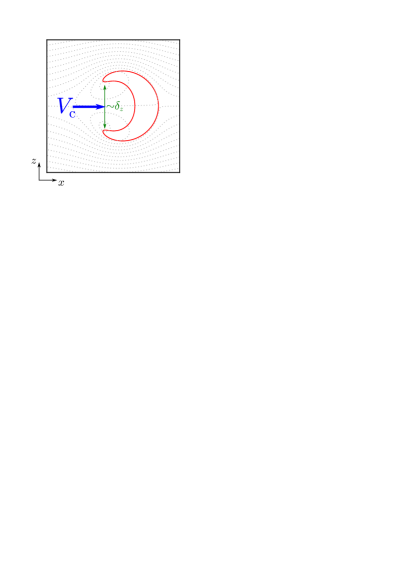
Figure 7: The stationary points of the flow (the dotted lines are streamlines of flow velocity in the frame of the filament) pin the ends of density contours which are ‘inflated’ by the flow between the stationary points, with velocity $\sim V_{\mathrm{c}}$

The filament increases its area because the crescent-shaped density contours are ‘inflated’ (since they cannot be compressed, their areas being preserved) by the flow on the axis, between the stagnation points of the circulating flow within the filament, which are separated by a distance $\sim\delta_{z}$, as illustrated in Figure 7. If the average velocity (in the filament frame) of that flow is $V_{\mathrm{c}}$ then

$$\frac{\partial\mathcal{A}}{\partial t}\sim V_{\mathrm{c}}\delta_{z}.$$ (6)

The only velocity scale in the system is $V_{\mathrm{f}}$, so (in the absence of any more exact calculation), we estimate $V_{\mathrm{c}}\sim V_{\mathrm{f}}$ so that

$$\frac{\partial P_{x}}{\partial t}\sim-L_{\|}\delta_{z}n_{0}V_{\mathrm{f}}^{2}.$$ (7)

The total force on the filament is in the positive $x$-direction, with magnitude ($\mathcal{F}$ denotes the filament region and $\partial\mathcal{F}$ its boundary)

$$-L_{\|}\int_{\mathcal{F}}d^{2}x\,J_{\mathrm{pol,}z}$$

$$=-L_{\|}\int_{\partial\mathcal{F}}ds\,z\hat{\boldsymbol{n}}\cdot\boldsymbol{J}_{\mathrm{pol}}+L_{\|}\int_{\mathcal{F}}d^{2}x\,z\nabla\cdot\boldsymbol{J}_{\mathrm{pol}}$$

$$=-L_{\|}\int_{\partial\mathcal{F}}ds\,z\hat{\boldsymbol{n}}\cdot\boldsymbol{J}_{\mathrm{pol}}-L_{\|}\int_{\mathcal{F}}d^{2}x\,z\nabla\cdot\boldsymbol{J}_{\mathrm{dia}}$$

$$=-L_{\|}\int_{\partial\mathcal{F}}ds\,z\hat{\boldsymbol{n}}\cdot\boldsymbol{J}_{\mathrm{pol}}-L_{\|}\int_{\mathcal{F}}d^{2}x\,zg\frac{\partial n}{\partial z}$$

$$=-L_{\|}\int_{\partial\mathcal{F}}ds\,z\hat{\boldsymbol{n}}\cdot\boldsymbol{J}_{\mathrm{pol}}-L_{\|}\int dx\left[zg\left(n-n_{0}\right)\right]_{z_{-}}^{z_{+}}+L_{\|}\int_{\mathcal{F}}d^{2}x\,g\left(n-n_{0}\right)$$

$$\approx gAL_{\|}n_{0}\delta_{x}\delta_{z}$$ (8)

integrating by parts twice. We may neglect the surface terms because firstly $\int_{\mathcal{E}}d^{2}x\,J_{\mathrm{pol,}z}\approx 0$ in the exterior region, $\mathcal{E}$, since the flow pattern is almost constant and so the external plasma must be close to global force balance. Since also $\nabla\cdot\boldsymbol{J}_{\mathrm{pol}}=0$ in the exterior region

$$0=\int_{\mathcal{E}}d^{2}x\,J_{\mathrm{pol},z}-\int_{\mathcal{E}}d^{2}x\,z\nabla\cdot\boldsymbol{J}_{\mathrm{pol}}=-\int_{\infty}ds\,z\hat{\boldsymbol{n}}\cdot\boldsymbol{J}_{\mathrm{pol}}+\int_{\partial\mathcal{F}}ds\,z\hat{\boldsymbol{n}}\cdot\boldsymbol{J}_{\mathrm{pol}}$$ (9)

and $\boldsymbol{J}_{\mathrm{pol}}$ vanishes at infinity ($r^{2}\boldsymbol{J}_{\mathrm{pol}}\rightarrow 0$ as $r\rightarrow\infty$ since otherwise the entire background plasma would accelerate). Secondly $(n-n_{0})\approx 0$ on the boundary, so $\int dx\left[zg\left(n-n_{0}\right)\right]_{z_{-}}^{z_{+}}\approx 0$, where $z_{+}$ and $z_{-}$ denote the upper and lower positions of the boundary at a particular $x$. The area integral is just the total number of particles in the perturbation, which is conserved from the initial state (and almost all contained within $\mathcal{F}$) and which we may estimate as

$$\int_{\mathcal{F}}d^{2}x\,\left(n-n_{0}\right)\sim An_{0}\delta_{x}\delta_{z}$$ (10)

where $A$ is the amplitude of the filament relative to the background and $\mathcal{A}\sim\delta_{x}\delta_{z}$ is the area of the filament (we assume that the changes in $\mathcal{A}$ with time are small compared to its magnitude).

Therefore the maximum filament velocity is attained when the rate of momentum gain from the exterior plasma, (7), balances the total force, (8), so

$$V_{\mathrm{f}}\sim\sqrt{gA\delta_{x}}$$ (11)

Parallel current

Linearising the sheath boundary condition,

$$\left.J_{\|}\right|_{\mathrm{sheath}}=\pm n_{\mathrm{sheath}}\left(1-e^{-\left.\phi\right|_{\mathrm{sheath}}}\right)\approx\pm n\phi$$ (12)

and integrating over $y$,

$$\int dy\,\nabla\cdot\boldsymbol{J}_{\|}\approx 2n\phi.$$ (13)

Since the filament velocity is approximately the central $\boldsymbol{E}\times\boldsymbol{B}$ velocity of the filament (in the lab frame), we can further estimate $V_{\mathrm{f}}\sim\phi/\delta_{z}$ and hence

$$\int dy\,\nabla\cdot\boldsymbol{J}_{\|}\sim n\delta_{z}V_{\mathrm{f}}.$$ (14)

So balancing this with the diamagnetic divergence, (3) (integrated over $y$), the velocity in this regime is

$$V_{\mathrm{f}}\sim\frac{L_{\|}g}{\delta_{z}^{2}}\frac{\left(n-n_{0}\right)}{n}\sim\frac{L_{\|}g}{\delta_{z}^{2}}\frac{A}{1+\beta A}.$$ (15)

The interpretation of the factor $\left(n-n_{0}\right)/n\sim A/\left(1+\beta A\right)$ and the value of the constant $\beta$ will be discussed in Section (2.2).

We have two regimes for filament dynamics, the inertial regime with maximum velocity given by (11) for narrow filaments and the sheath current regime with velocity given by (15) for wide filaments. Interestingly, the velocity depends on $\delta_{x}$ but not $\delta_{z}$ in the inertial regime and conversely on $\delta_{z}$ but not $\delta_{x}$ in the sheath current regime. The latter point was noted in the seminal paper [20], in the case without background plasma where a separable solution exists, but seems to have been neglected since then. The transition between the two regimens occurs when the velocities (11) and (15) are comparable, so

$$\sqrt{\delta_{x}}\delta_{z}^{2}\sim\sqrt{g}L_{\|}\frac{\sqrt{A}}{1+\beta A}.$$ (16)

2 Comparison with simulations

We have used two dimensional simulations to validate the scalings derived in Section 1.2. The equations used, based on those in [8], represent a filament assumed to have negligible variation along the magnetic field; closure is given by integrating the three dimensional system over the parallel direction to give equations for the density and vorticity

$$\frac{dn}{dt}=\hat{\boldsymbol{b}}\cdot\boldsymbol{g}\times\left(n\nabla\phi-\nabla n\right)+\frac{n\left(1-e^{-\phi}\right)}{L_{\|}}+\mu_{n}\nabla_{\perp}^{2}n$$ (17)

$$\frac{d\Omega}{dt}=-\frac{1}{2}\hat{\boldsymbol{b}}\cdot\nabla V_{E\times B}^{2}\times\nabla n-\hat{\boldsymbol{b}}\cdot\boldsymbol{g}\times\nabla n+\frac{n\left(1-e^{-\phi}\right)}{L_{\|}}+\mu_{\mathrm{i}}\nabla_{\perp}^{2}\Omega$$ (18)

$$\Omega=\nabla\cdot\left(n\nabla_{\perp}\phi\right)$$ (19)

with $d/dt=\left(\partial/\partial t+\hat{\boldsymbol{b}}\cdot\nabla\phi\times\nabla\right)$, $\boldsymbol{V}_{E\times B}=\hat{\boldsymbol{b}}\times\nabla\phi$ and, as before, $\boldsymbol{g}=g\hat{\boldsymbol{x}}$. (18) may be derived by taking the parallel component of the curl of the ion momentum equation

$$\frac{d\left(n\boldsymbol{V}_{\mathrm{i}}\right)}{dt}=\boldsymbol{J}_{\mathrm{pol}}\times\hat{\boldsymbol{b}}+\mu_{\mathrm{i}}\nabla_{\perp}^{2}\left(n\boldsymbol{V}_{\mathrm{i}}\right)$$ (20)

and replacing $\nabla\cdot\boldsymbol{J}_{\mathrm{pol}}$ using quasineutrality, $\nabla\cdot\boldsymbol{J}_{\mathrm{dia}}+\nabla\cdot\boldsymbol{J}_{\mathrm{pol}}+\nabla\cdot\boldsymbol{J}_{\|}=0$. (19) is inverted for $\phi$ using a new multigrid solver currently under development for BOUT++, to be reported elsewhere. The dimensionless parameters used are $L_{\|}=11000$, $g=2.5\times 10^{-3}$, $\mu_{n}=1.5\times 10^{-5}$ and $\mu_{\mathrm{i}}=4\times 10^{-4}$; for this theoretical study the dissipative parameters have been reduced by a factor of 100 compared to those used in [8], based on the expressions in [21], in order to minimise their effect on the inertial regime, since we do not treat viscosity here. Filaments are initialised as Gaussian density fluctuations with elliptical contours, tilted at an angle $\alpha$ to the $\hat{\boldsymbol{x}}$-direction, on a constant background,

$$n(t=0)=n_{0}\left(1+A\exp\left(-\frac{x^{\prime 2}/\epsilon+\epsilon z^{\prime 2}}{\delta^{2}}\right)\right)$$ (21)

where $A$ is the amplitude of the filament, $\epsilon$ is the ratio of the lengths of the axes of the ellipse, $\delta$ is the geometric mean of the lengths of the axes, $x^{\prime}=x\cos\alpha+z\sin\alpha$ and $z^{\prime}=z\cos\alpha-x\sin\alpha$.

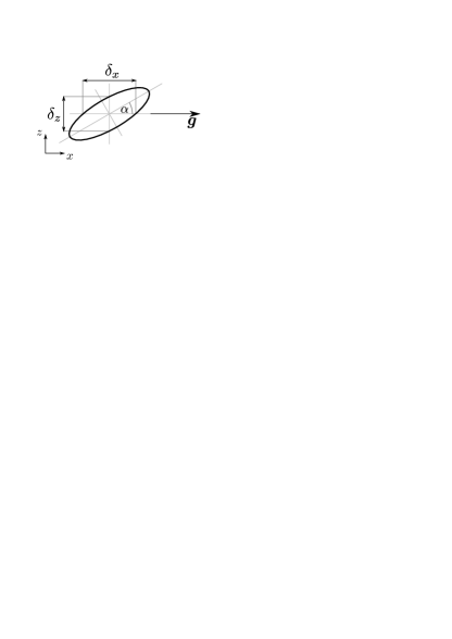
Figure 8: Schematic showing sizes and orientation of a tilted, elliptical filament cross-section

The diagram in figure 8 shows the configuration with the corresponding length scales, in the $\hat{\boldsymbol{x}}$- and $\hat{\boldsymbol{z}}$-directions respectively,

$$\delta_{x} =\delta\sqrt{\frac{\epsilon}{\left(\cos^{2}\alpha+\epsilon^{2}\sin^{2}\alpha\right)}}$$ (22)

$$\delta_{z} =\delta\sqrt{\frac{\epsilon}{\left(\epsilon^{2}\cos^{2}\alpha+\sin^{2}\alpha\right)}},$$ (23)

which appear in the velocity scaling above. Filament velocities are measured as the maximum velocity in the $\hat{\boldsymbol{x}}$-direction of the centre of mass of the density above background, i.e. $n-n_{0}$. These simulations, as well as the three dimensional ones in Section 3, have been implemented using BOUT++[22, 23].

2.1 Scaling with size and shape

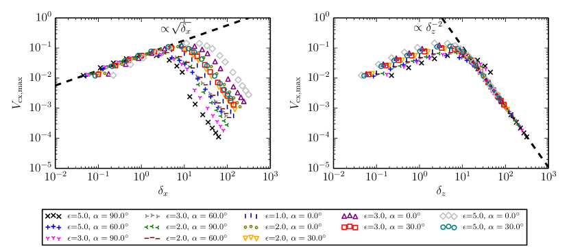
Figure 9: Inertial scaling vs. $\delta_{x}$ (left) and sheath current scaling vs. $\delta_{z}$ (right) with $A=4$ for several values of $\epsilon$ and $\alpha$

The results of a scan in width $\delta$, ellipticity $\epsilon$ and inclination $\alpha$, at constant amplitude $A=4$, are shown in Figure 9. For four different $\epsilon$ and four different $\alpha$, scanning $\delta$ results in a region of $\sqrt{\delta_{x}}$ scaling, corresponding to the inertial regime, and a region of $\delta_{z}^{-2}$ scaling corresponding to the sheath current regime. Moreover, although we have a three parameter space, $\{\delta,\epsilon,\alpha\}$, of filament sizes and shapes, a single combination ($\delta_{x}$ in the inertial regime and $\delta_{z}$ in the sheath current regime) entirely determines the filament velocity, at a particular amplitude (the effect of amplitude will be discussed in Section 2.2); this is evident from Figure 9 since all the points, for any $\epsilon$ and $\alpha$ (in the region where they follow $\sqrt{\delta_{x}}$ or $\delta_{z}^{-2}$ scaling) have not only the same gradient but also the same absolute magnitude.

The results for $\epsilon=3$, $\alpha=90^{\circ}$ and $\epsilon=5$, $\alpha=90^{\circ}$ exceed the $\delta_{z}^{-2}$ scaling for $\delta_{z}\approx 20-50$. This is due to the non-linearity of the sheath boundary condition which is included in the simulations, but not in the scaling. The maximum value of the potential is $\phi\approx 1.0$ at $\delta_{z}\approx 26$ for $\epsilon=3$ and $\phi\approx 1.0$ at $\delta_{z}\approx 34$ for $\epsilon=5$, so it makes sense that the deviation of $\exp\left(-\phi\right)$ from its linearised form is noticeable here. The effect of the non-linearity is to decrease the magnitude of the negative lobe of potential and increase the positive lobe. However, the enhancement of the positive lobe must be larger in order to allow the same magnitude, $j_{0}$, of current through the sheath: $\left|\phi_{+}\right|/\left|\phi_{-}\right|=-\ln\left(1-j_{0}\right)/\ln\left(1+j_{0}\right)>1$. The overall effect is therefore to increase the filament velocity, since the increase from the positive lobe outweighs the decrease from the negative lobe, resulting in a larger $E_{z}$.

The trend lines are $V\approx 5.7\times 10^{-2}\sqrt{\delta_{x}}$ for the inertial scaling and $V\approx 11\delta_{z}^{-2}$ for the sheath scaling. These intersect at $\delta_{z}^{4/5}\delta_{x}^{1/5}\approx 8.2$ whereas (16) suggests a crossover at $\delta_{z}^{4/5}\delta_{x}^{1/5}\approx 11.9$ for these parameters (using $\beta$ from Section (2.2)), in good agreement up to the order unity factors which are not fixed by analytical scaling arguments.

2.2 Amplitude scaling

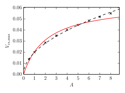
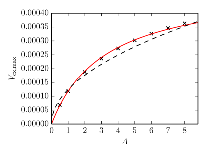
Figure 10: Amplitude scaling in the inertial regime, $\delta_{x}=\delta_{z}=0.5$, (left) and in the sheath current regime, $\delta_{x}=\delta_{z}=200$, (right). The solid red line shows the fitted ansatz, (24), and the dashed black line shows best fit line $\propto\sqrt{A}$

The amplitude scaling predicted for the inertial regime is simple, just $V\propto\sqrt{A}$, where the maximum fluctuation amplitude is $A=\max\left[\left(n-n_{0}\right)/n_{0}\right]$. For the sheath current regime the prediction is a little more complicated. We may estimate $\nabla_{z}(n-n_{0})\sim An_{0}/\delta_{z}$, but we need to find a representative value of $n$ to estimate $n^{-1}\nabla_{z}(n-n_{0})$ in (15). We find, by fitting the simulation results, that the appropriate value is neither the maximum, $n\sim(1+A)n_{0}$ nor the background $n\sim n_{0}$, but rather an intermediate value $n\sim(1+\beta A)n_{0}$, where $0<\beta<1$. $\beta$ corresponds to some point on the density profile at a distance $\tilde{\delta}_{z}$: $\beta=\exp(-\tilde{\delta}_{z}^{2}/\delta_{z}^{2})$. Then $V_{\mathrm{f}}$ as a function of $A$ with all other parameters held constant is

$$V_{\mathrm{f}}\propto\frac{A}{1+\beta A}$$ (24)

if the representative value of $n$ is found at the same relative position, $\tilde{\delta}_{z}/\delta_{z}$ for any $A$. This does indeed seem to be the case, as illustrated in Figure 10. For an amplitude scan with $\delta_{x}=\delta_{z}=0.5$, which is in the inertial regime $V\propto\sqrt{A}$ fits well, in agreement with [18], with $\varepsilon\approx 0.016$, where $\varepsilon$ is the root-mean-square relative error. For an amplitude scan with $\delta_{x}=\delta_{z}=200$, which is in the sheath current regime, (24) is a good fit, $\varepsilon\approx 0.014$, and gives $\beta\approx 0.31$. These conclusions also hold when varying the ellipticity, see A.

Comparing this to previous work: Angus and Krasheninnikov[18] established numerically the $\sqrt{A}$ scaling in the inertial regime, which we have tried to explain analytically above; Kube and Garcia[14] consider the amplitude dependence in some detail, where the scaling analysis starts from the vorticity equation and finds similar results to those given here, except that they use the Boussinesq approximation in their simulations and so do not find $\sqrt{A}$ in the inertial regime, while in the sheath current regime they assume a form equivalent to setting $\beta=1$ which prevents them from finding a quantitative, analytical amplitude scaling (their fit coefficients vary with amplitude, whereas here we have only a single, constant coefficient, $\beta$, to be derived from simulations); Angus et al.[6] give, albeit briefly, a derivation starting from the momentum equation, but neglect the amplitude dependence of the drive; Theiler et al.[17] in contrast use an interchange instability growth rate to estimate $\partial/\partial t\sim\gamma_{\mathrm{interchange}}$, and find a linear scaling with amplitude of the filament velocity in the inertial regime (which is contradicted here, emphasising that it is the non-linear, advective, term that is relevant); their derivation in [17] follows Garcia et al.[15, 24], but there the ‘ideal interchange rate’ is defined, without explanation, as

$$\gamma=\left(\frac{g}{\ell}\frac{\Delta\theta}{\Theta}\right)^{1/2}$$

(where $g$ corresponds to our $g$, $\ell$ to $L_{\|}$, $\Delta\theta$ is the fluctuation amplitude and $\Theta$ is the background density) which includes an amplitude dependence giving a square-root scaling of the filament velocity in the inertial regime.

3 Three Dimensional validation

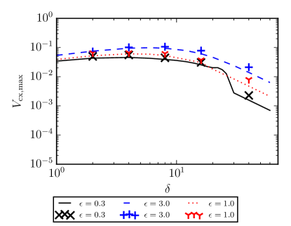
Figure 11: Comparison of two dimensional (lines) and three dimensional (markers) results for $A=2$ and several $\epsilon$

For reasons of computational expense, the three dimensional simulations in this section were done using the Boussinesq approximation (as were the two dimensional simulations just in this section, for consistency). This approximation is known to give the wrong amplitude scaling[18], but seems not to affect much the scaling with size and shape (at least the $\sqrt{\delta_{x}}$ inertial regime and $\delta_{z}^{-2}$ sheath current regime may be found either with or without the approximation). Here the normalised background density in the two dimensional simulations was set to $n_{0}\approx 1.48$ to be consistent with the (source-driven) background used for the three dimensional simulations, which normalise to the equilibrium density at the sheath entrance. The amplitude was set to a lower value than in the two dimensional case, $A=2$, to avoid the possibility of drift wave instabilities playing a role in the three dimensional simulations. For more details on the equations used in and implementation of the three dimensional simulations, see [8]. The three dimensional filaments were initialised with no variation in the parallel direction, in order to correspond to the two dimensional calculation as closely as possible; investigation of really ‘three dimensional’ effects due to parallel gradients is left for future work. Figure 11 shows that the three dimensional simulations follow the two dimensional trends closely.

The velocity of three dimensional filaments in the sheath current regime is slightly larger than the corresponding two dimensional ones. We attribute this to the variation in the background density: since this decreases near the sheath, the potential needed to drive the same sheath current is slightly increased and it follows that the filament velocity must then increase slightly.

The bump on the $\epsilon=1/3$ curve between $\delta=20$ and $\delta=30$, the part most affected by the non-linearity of the boundary condition (see Section 2.1), is due to the eventual fragmentation and subsequent acceleration of the filaments. In other words, it is due to their ceasing to travel as coherent structures and so its investigation is a subject beyond the scope of this paper.

4 Discussion

A number of works[16, 17] have analysed filament motion by analogy with the theory of linear instabilities; this has been termed the ‘blob correspondence principle’[16, 25]. Our analysis above shows that the picture is not quite so simple; the nature of the filaments as coherent, non-linear objects is important. Even in the sheath current regime, the density and potential fields have qualitatively different structures, being respectively monopolar and dipolar (Figure 3), rather than the identical structures, up to a phase shift, that they would have in linear theory; in the inertial regime the difference in the form of the fields from a simple mode structure is even more marked (Figures 4 and 5). Thus the nature of the physical processes involved in limiting filament velocity is clearer when considering the filament itself instead of analysing the governing equations by analogy or ‘correspondence’ to linear theory.

It is notable that in the inertial regime rather fine structures are formed, especially in the vorticity (see Figure 5). This suggests that both finite Larmor radius effects and viscosity may have significant effects on filaments in the inertial regime, which could provide an interesting topic for future study, perhaps using a gyrofluid model.

5 Conclusions

We have given here the first calculation of SOL filament velocity to include the effect of the filament shape and have also clarified the role of the filament amplitude. The analytical scaling calculations have been extensively validated by two dimensional simulation results, and also compared (with good agreement) to three dimensional simulations in which the filaments are initialised without parallel variation. Thus we now have a complete understanding of the mechanisms of filament propagation in the simple limit considered here. This understanding provides a solid foundation for the interpretation of filament motion in more complicated, more realistic models.

Appendix A Amplitude scaling fits

In order to verify that the form of the amplitude scaling is independent of the shape of the filament, we repeated the scans described in Section 2.2 for several different ellipticities, keeping $\delta_{x}$ constant for the filaments in the inertial regime and $\delta_{z}$ constant for the filaments in the sheath current regime so that (according to (11) and (15)) the velocities of the filaments should be independent of the ellipticity.

The root-mean-square relative error, $\varepsilon$, is defined by $\varepsilon^{2}=\frac{1}{N}\sum_{i}\frac{\left(V_{i}-V(A_{i})\right)^{2}}{V_{i}^{2}}$, where $V_{i}$ is the velocity measured from the simulation with amplitude $A_{i}$, $V(A)$ is the predicted scaling and $N$ is the number of simulations in the scan.

$\delta_{z}$	$\varepsilon$
$0.5/5$	0.052473
$0.5/3$	0.039863
$0.5/2$	0.029693
$0.5$	0.015660
$0.5\times 2$	0.022420
$0.5\times 3$	0.031436
$0.5\times 5$	0.044025

Table 1: Inertial regime: Comparison of $\varepsilon$ for the scaling $V\propto\sqrt{A}$ at $\delta_{x}=0.5$ for several values of $\delta_{z}$. Amplitudes used for the analysis were $A=1,1.5,2,3,4,5,6,7,8$.

$\delta_{x}$	$\beta$	$\varepsilon$
$200/5$	0.30985	0.014128
$200/3$	0.30994	0.014123
$200/2$	0.30997	0.014123
$200$	0.30999	0.014121
$200\times 2$	0.30999	0.014120
$200\times 3$	0.30999	0.014121
$200\times 5$	0.31000	0.014122

Table 2: Sheath current regime: Comparison of (i) values of $\beta$ inferred by least squares regression on the relative error between the ansatz (24) and filament velocities measured from simulations and (ii) values of $\varepsilon$ for this regression, at $\delta_{z}=200$ for several values of $\delta_{x}$. Amplitudes used for the analysis were $A=1,1.5,2,3,4,5,6,7,8$.

References

- [1] Ayed N B, Kirk A, Dudson B, Tallents S, Vann R G L, Wilson H R and the MAST team 2009 Plasma Physics and Controlled Fusion 51 035016 URL http://stacks.iop.org/0741-3335/51/i=3/a=035016
- [2] Boedo J A, Rudakov D L, Moyer R A, McKee G R, Colchin R J, Schaffer M J, Stangeby P G, West W P, Allen S L, Evans T E, Fonck R J, Hollmann E M, Krasheninnikov S, Leonard A W, Nevins W, Mahdavi M A, Porter G D, Tynan G R, Whyte D G and Xu X 2003 Physics of Plasmas 10 1670–1677 URL http://scitation.aip.org/content/aip/journal/pop/10/5/10.1063/1.1563259
- [3] Myra J, Davis W, D’Ippolito D, LaBombard B, Russell D, Terry J and Zweben S 2013 Nuclear Fusion 53 073013 URL http://stacks.iop.org/0029-5515/53/i=7/a=073013
- [4] Krasheninnikov S, D’Ippolito D and Myra J 2008 Journal of Plasma Physics 74(05) 679–717 ISSN 1469-7807 URL http://journals.cambridge.org/article_S0022377807006940
- [5] D’Ippolito D A, Myra J R and Zweben S J 2011 Physics of Plasmas 18 060501 URL http://scitation.aip.org/content/aip/journal/pop/18/6/10.1063/1.3594609
- [6] Angus J R, Krasheninnikov S I and Umansky M V 2012 Physics of Plasmas 19 082312 URL http://scitation.aip.org/content/aip/journal/pop/19/8/10.1063/1.4747619
- [7] Walkden N R, Dudson B D and Fishpool G 2013 Plasma Physics and Controlled Fusion 55 105005 URL http://stacks.iop.org/0741-3335/55/i=10/a=105005
- [8] Easy L, Militello F, Omotani J, Dudson B, Havlíčková E, Tamain P, Naulin V and Nielsen A H 2014 Physics of Plasmas 21 122515 URL http://scitation.aip.org/content/aip/journal/pop/21/12/10.1063/1.4904207
- [9] Madsen J, Garcia O E, Stærk Larsen J, Naulin V, Nielsen A H and Rasmussen J J 2011 Physics of Plasmas 18 112504 URL http://scitation.aip.org/content/aip/journal/pop/18/11/10.1063/1.3658033
- [10] Ricci P and Rogers B N 2013 Physics of Plasmas 20 010702 URL http://scitation.aip.org/content/aip/journal/pop/20/1/10.1063/1.4789551
- [11] Militello F, Tamain P, Fundamenski W, Kirk A, Naulin V, Nielsen A H and the MAST team 2013 Plasma Physics and Controlled Fusion 55 025005 URL http://stacks.iop.org/0741-3335/55/i=2/a=025005
- [12] Tamain P, Ghendrih P, Bufferand H, Ciraolo G, Colin C, Fedorczak N, Nace N, Schwander F and Serre E 2015 Plasma Physics and Controlled Fusion 57 054014 URL http://stacks.iop.org/0741-3335/57/i=5/a=054014
- [13] Easy L, Militello F, Walkden N, Omotani J and Dudson B 2015 submitted to Physics of Plasmas
- [14] Kube R and Garcia O E 2011 Physics of Plasmas 18 102314 URL http://scitation.aip.org/content/aip/journal/pop/18/10/10.1063/1.3647553
- [15] Garcia O E, Bian N H, Naulin V, Nielsen A H and Rasmussen J J 2005 Physics of Plasmas 12 090701 URL http://scitation.aip.org/content/aip/journal/pop/12/9/10.1063/1.2044487
- [16] Myra J R and D’Ippolito D A 2005 Physics of Plasmas 12 092511 URL http://scitation.aip.org/content/aip/journal/pop/12/9/10.1063/1.2048847
- [17] Theiler C, Furno I, Ricci P, Fasoli A, Labit B, Müller S H and Plyushchev G 2009 Phys. Rev. Lett. 103(6) 065001 URL http://link.aps.org/doi/10.1103/PhysRevLett.103.065001
- [18] Angus J R and Krasheninnikov S I 2014 Physics of Plasmas 21 112504 URL http://scitation.aip.org/content/aip/journal/pop/21/11/10.1063/1.4901237
- [19] Russell D A, D’Ippolito D A, Myra J R, Nevins W M and Xu X Q 2004 Phys. Rev. Lett. 93(26) 265001 URL http://link.aps.org/doi/10.1103/PhysRevLett.93.265001
- [20] Krasheninnikov S 2001 Physics Letters A 283 368 – 370 ISSN 0375-9601 URL http://www.sciencedirect.com/science/article/pii/S0375960101002523
- [21] Fundamenski W, Garcia O, Naulin V, Pitts R, Nielsen A, Rasmussen J J, Horacek J, Graves J and contributors J E 2007 Nuclear Fusion 47 417 URL http://stacks.iop.org/0029-5515/47/i=5/a=006
- [22] Dudson B, Umansky M, Xu X, Snyder P and Wilson H 2009 Computer Physics Communications 180 1467 – 1480 ISSN 0010-4655 URL http://www.sciencedirect.com/science/article/pii/S0010465509001040
- [23] Dudson B D, Allen A, Breyiannis G, Brugger E, Buchanan J, Easy L, Farley S, Joseph I, Kim M, McGann A D, Omotani J T, Umansky M V, Walkden N R, Xia T and Xu X Q 2015 Journal of Plasma Physics 81(01) ISSN 1469-7807 URL http://journals.cambridge.org/article_S0022377814000816
- [24] Garcia O E, Bian N H and Fundamenski W 2006 Physics of Plasmas 13 082309 URL http://scitation.aip.org/content/aip/journal/pop/13/8/10.1063/1.2336422
- [25] Myra J R, Russell D A and D’Ippolito D A 2006 Physics of Plasmas 13 112502 URL http://scitation.aip.org/content/aip/journal/pop/13/11/10.1063/1.2364858