Large deviations and rain showers

Abstract

Rainfall from ice-free cumulus clouds requires collisions of large numbers of microscopic droplets to create every raindrop. The onset of rain showers can be surprisingly rapid, much faster than the mean time required for a single collision. Large-deviation theory is used to explain this observation.

The dynamics of the onset of rainfall from ice-free (‘warm’) cumulus clouds is poorly understood Mas71 ; Pru+97 ; Sha03 . A rain drop grows by collisions of microscopic water droplets. A large number of microscopic droplets must combine to make one rain drop: the volume increase is a factor of approximately one million. The collision rates in the early stages of the growth process are low (typically of order one collision per hour). Given the large number of collisions which must occur, it is very hard to understand the observation that rain showers can be initiated over relatively short periods, of perhaps twenty minutes.

One possible resolution is a consequence of the large number of microscopic droplets which must combine to make a raindrop. This implies that only very few drops are required to undergo explosive growth, and perhaps there are sufficient rare combinations of rapid multiple collisions to explain rainfall: this point has previously been emphasised by Kostinski and Shaw Kos+05 . A quantitative approach is required to show whether the large number of collisions required for runaway growth can occur with a sufficiently high probability. Because this problem involves the analysis of rare events, methods based upon large deviation theory Fre+84 ; Tou09 are used in this Letter to investigate the hypothesis that rare combinations of rapid collisions trigger showers. It is shown that a rain shower can develop over a timescale which is a small fraction of the mean timescale for one collision.

First, consider some observations and estimates Mas71 ; Pru+97 ; Sha03 which illustrate the difficulties in making a quantitative description of rainfall. A convecting cumulus cloud which could produce showers may have droplets of mean radius radius is $a_{0}=10\,\mu{\rm m}$, which result from condensation onto aerosol nuclei. Raindrops have a much larger size, typically $1\,{\rm mm}$. The volume of a droplet which becomes a raindrop therefore increases by a very large factor, denoted by ${\cal N}$, which is typically ${\cal N}\approx 10^{6}$. The number density of microscopic droplets is typically of order $N_{0}=2.5\times 10^{8}\,{\rm m}^{-3}$, which gives a liquid water content, expressed as a volume fraction, $\Phi_{\rm l}\approx 4\pi N_{0}a_{0}^{3}/3\approx 10^{-6}$. The cloud depth may be $h=2\times 10^{3}\,{\rm m}$ and the typical vertical velocity of air inside the cloud has magnitude $U\approx 2\,{\rm m}\,{\rm s}^{-1}$, so that the turnover time for convection is approximately $\tau_{h}=10^{3}\,{\rm s}$. Rainfall from this type of cloud can develop over a timescale of approximately $20\,{\rm min}\approx 10^{3}\,{\rm s}$.

Droplets which undergo a geometrical collision (the impact parameter is less than the sum of the radii) might not coalesce, because the streamlines of small droplets curve around larger ones. In fact, if the Navier-Stokes equations were a complete description, droplets would never collide, because there would always be a lubricating film of air between them. The coalescence efficiencies $\varepsilon$ of small droplets are somewhat uncertain, but it is widely accepted that they are low for typical cloud droplets Mas71 ; Pru+97 . If the larger droplet has radius below $20\,\mu{\rm m}$, it is believed that $\varepsilon\leq 0.1$, and that for radius $10\,\mu{\rm m}$, $\varepsilon\leq 0.03$ Pru+97 . For droplets of size $a=50\,\mu{\rm m}$ colliding with droplets of size $a=10\,\mu{\rm m}$, however, the efficiencies are expected to be close to unity Pru+97 ; Mas71 .

Collisions between droplets settling at a different rate yield a very small collision rate. The Stokes law for the drag on a sphere at low Reynolds number indicates that the gravitational settling rate is

$$v=\tau_{\rm p}g=\kappa a^{2}\ ,\ \ \ \kappa=\frac{2}{9}\frac{\rho_{\rm l}}{\rho_{\rm g}}\frac{g}{\nu}$$ (1)

where $\tau_{\rm p}$ is the response time characterising the Stokes drag on a droplet, $\rho_{\rm l}$ is the density of liquid water, and $\rho_{\rm g}$ and $\nu$ are, respectively, the density and kinematic viscosity of air. Inserting values for air and water at $5^{\circ}{\rm C}$ gives $\kappa\approx 1.4\times 10^{8}\,{\rm m}^{-1}{\rm s}^{-1}$, so that when $a_{0}=10\,\mu{\rm m}$ the terminal velocity is $v\approx 1.4\times 10^{-2}\,{\rm ms}^{-1}$ and the response time is $1.4\times 10^{-3}\,{\rm s}$. The collision rate of a drop of radius $a_{1}$ with a gas of droplets of radius $a_{0}$ is

$$R_{1}=\pi\varepsilon N_{0}(a_{0}+a_{1})^{2}\kappa(a_{1}^{2}-a_{0}^{2})$$ (2)

where $\varepsilon$ is the collision efficiency. Setting $a_{1}-a_{0}=2.5\,\mu{\rm m}$ and $\varepsilon=0.03$ in addition to the parameters defined above gives $R_{1}\approx 2\times 10^{-5}{\rm s}^{-1}$. The rate of coalescence of typical sized water droplets due to collisions is therefore very small.

Cumulus clouds are turbulent because of convective instability. Saffman and Turner Saf+56 investigated the role of turbulence in facilitating collisions between water droplets. In the case of very small droplets, the collision rate due to turbulence is a consequence of shearing motion. The shear rate of small-scale motions in turbulence is the inverse of the Kolmogorov timescale, $\tau_{\rm K}=\sqrt{\nu/\epsilon}$, where $\epsilon$ is the rate of dissipation per unit mass. According to the Saffman-Turner model, shear induces a collision speed of order $a_{0}/\tau_{\rm K}$. They argue that the corresponding collision rate is

$$R_{\rm turb}=\sqrt{\frac{8\pi}{15}}\frac{N_{0}\varepsilon(2a)^{3}}{\tau_{\rm K}}\ .$$ (3)

For the parameters of the cloud model, the rate of dissipation is $\epsilon\sim U^{2}/\tau_{h}\approx 2\times 10^{-3}\,{\rm m}^{2}{\rm s}^{-3}$, giving $\tau_{\rm K}\approx 70\,{\rm ms}$, which gives $R_{\rm turb}\approx 10^{-6}\,{\rm s}^{-1}$, which is negligible. The effects of turbulence are dramatically increased when the effects of droplet inertia are significant: this was noticed in numerical experiments by Sundaram and Collins Sun+97 , who ascribed the effect to a clustering effect termed ‘preferential concentration’ Max87 . More recent work has proposed an alternative mechanism, which has been termed the ‘sling effect’ Fal+02 , and which has been explained in terms of the existence of caustics in the velocity field of the droplets Wil+06 . Inertial effects are measured by the Stokes number, ${\rm St}\equiv\tau_{\rm p}/\tau_{\rm K}$. Recent numerical studies Vos+14 (see also Gra+13 ) show that the collision rate is greatly enhanced by effects due to caustics for ${\rm St}>0.3$, equation (3) is a good estimate when ${\rm St}\ll 1$. While it is in principle possible for turbulence to be responsible for an enhanced collision rate of water droplets due to inertial effects, the parameters of the cloud model discussed above yield ${\rm St}\approx 2\times 10^{-2}$, where there is no significant enhancement. While there is a consensus that turbulence is important for the formation of rain showers Bod+10 , turbulent enhancement of collision rates does not appear to be sufficient.

Now consider how to model the onset of a shower. It has already been remarked that showers occur on a timescale which may be smaller than the typical timescale for one collision. It is, therefore, reasonable to assume that the runaway droplets are falling through a background of droplets which have not yet coalesced. As a runaway droplet falls it collides with a large number ${\cal N}$ of small droplets of size $a_{0}$. The time between successive collisions may be assumed to be independent Poisson processes. If the time between the collision with index $n$ and the previous collision is $t_{n}$, the time for a droplet to experience runaway growth is

$$T=\sum_{i=1}^{\cal N}t_{n}$$ (4)

where the $t_{n}$ are independent random variables with a Poisson distribution

$$P_{n}(t_{n})=R_{n}\exp(-R_{n}t_{n})\ .$$ (5)

The problem is to determine the statistics of $T$ in the limit as ${\cal N}\to\infty$. The rates for successive collisions increase as the size of the falling drop grows. Because all of the collision rates $R_{n}$ scale in the same way as a function of the droplet size $a_{0}$ and the number density $N_{0}$, write

$$R_{n}=R_{1}f(n)\ .$$ (6)

Here $R_{1}$ depends upon the properties of the cloud but the function $f(n)$ is the same for all clouds. In order to identify the form of $f(n)$, consider the rate of collision of a large droplet resulting from $n$ previous collisions with a gas of small droplets of radius $a_{0}$. The radius of the large droplet is $a_{n}=n^{1/3}a_{0}$. When $n$ is large it may assumed that the collision efficiency is $\varepsilon\approx 1$ and $a_{n}\gg a_{0}$ so that $R_{n}\sim\pi N_{0}\kappa a_{n}^{4}\propto n^{4/3}$, which suggests setting $f(n)=n^{4/3}$. However during the early stages of droplet growth, the collision efficiency for the first few collisions is small, but increases rapidly with $n$. In what follows $f(n)$ is assumed to be a power-law

$$R_{n}=R_{1}n^{\gamma}\ .$$ (7)

If the collision efficiency of droplets were unity, it would be appropriate to set $\gamma=4/3$. Because the collision efficiency of droplets at the crucial initial stage of their growth is small, the collision rate increases more rapidly as the size of the falling droplet increases. When the droplets are between $10\,\mu{\rm m}$ and $50\,\mu{\rm m}$ it is reasonable to model the product of the collision rate and the collision efficiency as being proportional to $a^{6}$, that is to $n^{2}$, where $n$ is the number of collisions Kos+05 . In other cases, such as solid precipitation (snow), other values of $\gamma$ may be appropriate. In the following $\gamma$ is left as an adjustable parameter, but special consideration is given to $\gamma=2$, because it gives a good approximation to terrestrial rainfall, and to $\gamma=4/3$, because this may be a good approximation for atmospheres on other planets where the collision efficiency might not limit the rate of coalescence.

It is necessary to determine the probability density for the time $T$ being a very small fraction of its mean value, $\langle T\rangle$. Inspired by large deviation theory Fre+84 ; Tou09 , the probability density of $T$ is written in an exponential form:

$$P(T)=\frac{1}{\langle T\rangle}\exp[-J(\tau)]\ ,\ \ \ \ \tau=\frac{T}{\langle T\rangle}\ .$$ (8)

When $f(n)$ is given by (7), the mean time for explosive growth converges as ${\cal N}\to\infty$ when $\gamma>1$:

$$\lim_{{\cal N}\to\infty}\langle T\rangle=\lim_{{\cal N}\to\infty}\frac{1}{R_{1}}\sum_{n=1}^{\cal N}\frac{1}{f(n)}=\frac{1}{R_{1}}\zeta(\gamma)\ .$$ (9)

where $\zeta$ is the Riemann zeta function. The function $J(\tau)$ in (8) is often termed the entropy in texts on large deviation theory. It will be necessary to determine the entropy function $J(\tau)$ from the rate function $f(n)$.

After a drop has grown to a size where it is much larger than the typical droplets, and where the collision efficiency is approximately unity, it falls rapidly and collects other droplets in its path. Consider a drop of size $a_{1}$ falling through a ‘gas’ of much smaller droplets, with liquid volume fraction $\Phi_{\rm l}$. The larger drop falls with velocity $v=\kappa a_{1}^{2}$ and grows in volume at a rate $\pi\varepsilon a_{1}^{2}\Phi_{\rm l}v=4\pi a_{1}^{2}\dot{a}_{1}$, where $\dot{a}_{1}$ is the rate of increase of the drop radius. The rate of increase of the radius of the ‘collector’ drop as a function of the distance $x$ through which it has fallen is

$$\frac{{\rm d}a}{{\rm d}x}=\frac{\varepsilon\Phi_{\rm l}}{4}\ .$$ (10)

Note that this expression is valid whether or not the terminal velocity is given by the small Reynolds number approximation, (1). In the case of droplets which reach a radius of approximately $1\,{\rm mm}$, the collision efficiency $\varepsilon$ is close to unity throughout most of the fall. The droplet radius after falling through a cloud of depth $h$ is therefore $a(h)\sim\Phi_{\rm l}h/4$. It will be assumed that the most relevant collector drops are those that started at the top of the cloud, so that the volumetric growth factor is

$${\cal N}=\left(\frac{h}{4a_{0}}\right)^{3}\Phi_{\rm l}^{3}\ .$$ (11)

Using the representative values given above gives ${\cal N}\approx 10^{5}$.

The rate of change of the liquid water content of a cloud due to the runaway growth of droplets is

$$\frac{{\rm d}\Phi_{\rm l}}{{\rm d}t}=-\Phi_{\rm l}{\cal N}P(t)\ .$$ (12)

Note that the growth factor ${\cal N}$ and the probability density for runaway growth after time $t$ are both functions of $\Phi_{\rm l}$, but if the objective is to understand the onset of a rain shower it suffices to evaluate these quantities with the initial value $\Phi_{\rm l}(0)$. Using (8) for $P(t)$, the condition for the timescale $t^{\ast}$ where there is a significant reduction in $\Phi_{\rm l}(t)$ is ${\cal N}\exp[-J(t^{\ast}/\langle T\rangle)]=1$, that is

$$t^{\ast}=\tau^{\ast}\langle T\rangle\ ,\ \ \ \ J(\tau^{\ast})={\rm ln}\,{\cal N}\ .$$ (13)

The droplet volume growth factor ${\cal N}$ was estimated in equation (11). To determine determine the solution of (13) for $t^{\ast}$, it is necessary to determine the entropy function $J(\tau)$ for the random sum defined by (4) and (5).

To compute $J(T)$ consider a cumulent generating function $\lambda(k)$, defined by writing

$$\exp[-\lambda(k)]=\langle\exp(-kT)\rangle=\int_{0}^{\infty}{\rm d}T\ P(T)\,\exp(-kT)\ .$$ (14)

Because the $t_{n}$ are independent, with a distribution given by (5):

$$\lambda(k)=\sum_{n=1}^{\cal N}{\rm ln}\langle\exp(-kt_{n})\rangle=\sum_{n=1}^{\cal N}{\rm ln}\left(1+\frac{k}{R_{n}}\right)\ .$$ (15)

Now consider how to obtain $P(T)$ from $\lambda(k)$. Noting that $\exp[-\lambda(k)]$ is the Laplace transform of $P(T)$, application of the Bromwich integral formula for inversion gives

$$P(T)=\frac{1}{2\pi{\rm i}}\int_{C-{\rm i}\infty}^{C+{\rm i}\infty}{\rm d}z\ \exp[zT-\lambda(z)]$$ (16)

where $C>-R_{1}$. The integral is dominated by contributions from the neighbourhood of a saddle at $z=k^{\ast}$, where

$$T=\sum_{n=1}^{\cal N}\frac{1}{R_{n}+k^{\ast}}$$ (17)

which is to be solved for $k^{\ast}$ given a value of $T$. The probability density $P(T)$ is then approximated by

$$P(T)=\frac{1}{R_{1}}\frac{1}{\sqrt{2\pi{\cal S}(k^{\ast})}}\exp[-J(\tau)]$$ (18)

where $\tau=T/\langle T\rangle$ and ${\cal S}(k)$ is the magnitude of the second derivative of the exponent in (16). Equations (17) and (18) cannot be solved exactly and explicitly for $J(\tau)$. Consider how to write down a parametric representation of $J(\tau)$ using a scaled variable, $\kappa$, defined by $\kappa=k^{\ast}/R_{1}$. The dimensionless time for raindrop formation is

$$\tau(\kappa)=\sum_{n=1}^{\cal N}\frac{1}{\kappa+n^{\gamma}}\left[{\sum_{n=1}^{\cal N}n^{-\gamma}}\right]^{-1}$$ (19)

and the entropy function is

$$J(\kappa)=\sum_{n=1}^{\cal N}{\rm ln}\left(1+\kappa n^{-\gamma}\right)-\sum_{n=1}^{\cal N}\frac{\kappa n^{-\gamma}}{1+\kappa n^{-\gamma}}\ .$$ (20)

Figure 1 shows the distribution of $\tau=T/\langle T\rangle$ for the case $\gamma=4/3$, with ${\cal N}=4000$ and $R_{1}=1$, comparing the results of simulation of (4), the Bromwich integral (16), the saddle-point approximation, equations (18), (19), (20), which are all in excellent agreement. Figure 2 makes a similar comparison for the case $\gamma=2$, which is most relevant to rain showers. In both cases the entropy function increases very rapidly as $\tau\to 0$, indicating that the value of $\tau^{\ast}=t^{\ast}/\langle T\rangle$ is quite insensitive to the value of ${\rm ln}\,{\cal N}$. It is clear from figure 2 that the solution of equation (13) gives small values of $\tau^{\ast}$ when ${\cal N}$ is large. Numerical evaluation of (16) with $\gamma=2$ gives $\tau^{\ast}\approx 0.077$ when ${\cal N}=10^{5}$ and $\tau^{\ast}\approx 0.068$ when ${\cal N}=10^{6}$. Alternatively, in terms of $\langle t_{1}\rangle=\langle T\rangle/\zeta(\gamma)$, when $\gamma=2$, the predicted time for onset of a shower is a small fraction of the mean time for the first collision: $t^{\ast}\approx 0.128\langle t_{1}\rangle$ when ${\cal N}=10^{5}$ and $t^{\ast}\approx 0.112\langle t_{1}\rangle$ when ${\cal N}=10^{6}$.

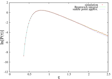
Figure 1: Plot of ${\rm ln}[P(\tau)]$, for ${\cal N}=4000$ and $\gamma=4/3$. The results of simulation, evaluation of the Bromwich integral, and the saddle point approximation are in excellent agreement.

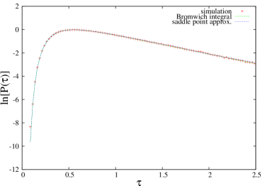
Figure 2: Plot of ${\rm ln}[P(\tau)]$, for ${\cal N}=4000$ and $\gamma=2$.

It is clear from figures 1 and 2 that the entropy increases very rapidly as $\tau\to 0$, and it is desirable to find asymptotic behaviour of $J(\tau)$ when $\tau\ll 1$. This limit corresponds to $\kappa\gg 1$. In the limit where ${\cal N}\to\infty$ and $\kappa\gg 1$ in equations (19) and (20), the sum in the numerator of (19) is approximated by an integral:

$$\tau(\kappa)\sim\frac{1}{\zeta(\gamma)}\int_{0}^{\infty}{\rm d}n\ \frac{1}{\kappa+n^{\gamma}}=\kappa^{\frac{1}{\gamma}-1}F(\gamma)$$ (21)

with

$$F(\gamma)=\frac{1}{\gamma\zeta(\gamma)}\int_{0}^{\infty}{\rm d}x\ \frac{x^{\frac{1}{\gamma}-1}}{1+x}\ .$$ (22)

A similar approach applied to (20) gives

$$J(\kappa)=\kappa^{\frac{1}{\gamma}}G(\gamma)\ ,\ \ \ G(\gamma)=\frac{1}{\gamma}\int_{0}^{\infty}{\rm d}x\ \frac{{\rm ln}(1+x)}{x^{\frac{1}{\gamma}+1}}-\zeta(\gamma)F(\gamma)\ .$$ (23)

Eliminating $\kappa$ from (22) an (23) shows that in the limit as $\tau\to 0$ the entropy function has a power-law divergence: to leading order

$$J(\tau)\sim G(\gamma)[F(\gamma)]^{\frac{1}{\gamma-1}}\tau^{-\frac{1}{\gamma-1}}\equiv K(\gamma)\tau^{-\frac{1}{\gamma-1}}\ .$$ (24)

This indicates that the probability density has a non-algebraic singularity as $\tau\to 0$: $P(\tau)\sim\exp(-K/\tau)$ when $\gamma=2$, or $P(\tau)\sim\exp(-K/\tau^{3})$ when $\gamma=\tfrac{4}{3}$. Numerical integration gives $K(\tfrac{4}{3})\approx 0.8799$, whereas $K(2)=\pi^{2}/4\zeta(2)=\tfrac{3}{2}$ exactly.

The conclusion is that rain showers can commence in a timescale which is short compared to the mean time for the first collision between droplets, with the timescale for onset being approximately one eighth of the mean time for first collision in the case of the more realistic model ($\gamma=2$). Thus large deviation theory has resolved an apparent paradox of meteorology, that rain showers can start very quickly, on timescale which are short compared to typical mean collision times.

This calculation does not resolve all of the uncertainties about initiation of rain showers. Clouds can exist for a long period without producing a rain shower, before depositing a large fraction of their water content over a short time. Shower activity is associated with convective motion in clouds, and it has been suggested that turbulence facilitates collisions. For typical levels of turbulence, however, turbulent enhancement of collisions does not appears to be sufficient. It seems as if non-collisional mechanisms involving convection must may a role in initiating the cascade Wil14 .

This work was initiated during a visit to the Kavli Institute for Theoretical Physics, Santa Barbara, where this research was supported in part by the National Science Foundation under Grant No. NSF PHY11-25915.

References

- (1) B. J. Mason, The Physics of Clouds, 2nd. ed., Oxford, University Press, (1971).
- (2) H. R. Pruppacher and J. D. Klett, Microphysics of Clouds and Precipitation, 2nd ed., Dordrecht, Kluwer, (1997).
- (3) R. A. Shaw, Ann. Rev. Fluid Mech., 35, 183-227, (2003).
- (4) A.B. Kostinski and R.A. Shaw, Bull. Am. Met. Soc., 86, 235-244, (2005).
- (5) M. I. Freidlin and A. D. Wentzell, Random Perturbations of Dynamical Systems, Grundlehren der Mathematischen Wissenschaften, vol. 260, Springer, New York, (1984).
- (6) H. Touchette, The large deviation approach to statistical mechanics, Phys. Rep., 478, 1-69, (2009).
- (7) P. G. Saffamn and J. S. Turner, J. Fluid Mech., 1, 16-30, (1956).
- (8) S. Sundaram and L. R. Collins, J. Fluid Mech , 335, 75, (1997).
- (9) M. R. Maxey, J. Fluid Mech., 174, 441-65, (1987).
- (10) G. Falkovich, A. Fouxon and M. G. Stepanov, Nature, 419, 151-4, (2002).
- (11) M. Wilkinson, B, Mehlig and V. Bezuglyy, Phys. Rev. Lett., 97, 048501, (2006).
- (12) M. Voßkuhle, A. Pumir, E. Lévêque and M. Wilkinson, J. Fluid Mech., 749, 841-852, (2014).
- (13) W. W. Grabowski and L. P. Wang, Annu. Rev. Fluid Mech, 45, 293-324, (2013).
- (14) E. Bodenschatz, S. P. Malinowski, R. A. Shaw and F. Stratmann, Science. 327, 970-71, (2010).
- (15) M. Wilkinson, Europhys. Lett., 108, 49001, (2014).