Non-parametric Revenue Optimization for Generalized Second Price Auctions

Abstract

We present an extensive analysis of the key problem of learning optimal reserve prices for generalized second price auctions. We describe two algorithms for this task: one based on density estimation, and a novel algorithm benefiting from solid theoretical guarantees and with a very favorable running-time complexity of $O(nS\log(nS))$, where $n$ is the sample size and $S$ the number of slots. Our theoretical guarantees are more favorable than those previously presented in the literature. Additionally, we show that even if bidders do not play at an equilibrium, our second algorithm is still well defined and minimizes a quantity of interest. To our knowledge, this is the first attempt to apply learning algorithms to the problem of reserve price optimization in GSP auctions. Finally, we present the first convergence analysis of empirical equilibrium bidding functions to the unique symmetric Bayesian-Nash equilibrium of a GSP.

1 INTRODUCTION

The Generalized Second-Price (GSP) auction is currently the standard mechanism used for selling sponsored search advertisement. As suggested by the name, this mechanism generalizes the standard second-price auction of Vickrey (1961) to multiple items. In the case of sponsored search advertisement, these items correspond to ad slots which have been ranked by their position. Given this ranking, the GSP auction works as follows: first, each advertiser places a bid; next, the seller, based on the bids placed, assigns a score to each bidder. The highest scored advertiser is assigned to the slot in the best position, that is, the one with the highest likelihood of being clicked on. The second highest score obtains the second best item and so on, until all slots have been allocated or all advertisers have been assigned to a slot. As with second-price auctions, the bidder’s payment is independent of his bid. Instead, it depends solely on the bid of the advertiser assigned to the position below.

In spite of its similarity with second-price auctions, the GSP auction is not an incentive-compatible mechanism, that is, bidders have an incentive to lie about their valuations. This is in stark contrast with second-price auctions where truth revealing is in fact a dominant strategy. It is for this reason that predicting the behavior of bidders in a GSP auction is challenging. This is further worsened by the fact that these auctions are repeated multiple times a day. The study of all possible equilibria of this repeated game is at the very least difficult. While incentive compatible generalizations of the second-price auction exist, namely the Vickrey-Clark-Gloves (VCG) mechanism, the simplicity of the payment rule for GSP auctions as well as the large revenue generated by them has made the adoption of VCG mechanisms unlikely.

Since its introduction by Google, GSP auctions have generated billions of dollars across different online advertisement companies. It is therefore not surprising that it has become a topic of great interest for diverse fields such as Economics, Algorithmic Game Theory and more recently Machine Learning.

The first analysis of GSP auctions was carried out independently by Edelman et al. (2005) and Varian (2007). Both publications considered a full information scenario, that is one where the advertisers’ valuations are publicly known. This assumption is weakly supported by the fact that repeated interactions allow advertisers to infer their adversaries’ valuations. Varian (2007) studied the so-called Symmetric Nash Equilibria (SNE) which is a subset of the Nash equilibria with several favorable properties. In particular, Varian showed that any SNE induces an efficient allocation, that is an allocation where the highest positions are assigned to advertisers with high values. Furthermore, the revenue earned by the seller when advertisers play an SNE is always at least as much as the one obtained by VCG. The authors also presented some empirical results showing that some bidders indeed play by using an SNE. However, no theoretical justification can be given for the choice of this subset of equilibria (Börgers et al., 2013; Edelman and Schwarz, 2010). A finer analysis of the full information scenario was given by Lucier et al. (2012). The authors proved that, excluding the payment of the highest bidder, the revenue achieved at any Nash equilibrium is at least one half that of the VCG auction.

Since the assumption of full information can be unrealistic, a more modern line of research has instead considered a Bayesian scenario for this auction. In a Bayesian setting, it is assumed that advertisers’ valuations are i.i.d. samples drawn from a common distribution. Gomes and Sweeney (2014) characterized all symmetric Bayes-Nash equilibria and showed that any symmetric equilibrium must be efficient. This work was later extended by Sun et al. (2014) to account for the quality score of each advertiser. The main contribution of this work was the design of an algorithm for the crucial problem of revenue optimization for the GSP auction. Lahaie and Pennock (2007) studied different squashing ranking rules for advertisers commonly used in practice and showed that none of these rules are necessarily optimal in equilibrium. This work is complemented by the simulation analysis of Vorobeychik (2009) who quantified the distance from equilibrium of bidding truthfully. Lucier et al. (2012) showed that the GSP auction with an optimal reserve price achieves at least 1/6 of the optimal revenue (of any auction) in a Bayesian equilibrium. More recently, Thompson and Leyton-Brown (2013) compared different allocation rules and showed that an anchoring allocation rule is optimal when valuations are sampled i.i.d. from a uniform distribution. With the exception of Sun et al. (2014), none of these authors have proposed an algorithm for revenue optimization using historical data.

Zhu et al. (2009) introduced a ranking algorithm to learn an optimal allocation rule. The proposed ranking is a convex combination of a quality score based on the features of the advertisement as well as a revenue score which depends on the value of the bids. This work was later extended in (He et al., 2014) where, in addition to the ranking function, a behavioral model of the advertisers is learned by the authors.

The rest of this paper is organized as follows. In Section 2, we give a learning formulation of the problem of selecting reserve prices in a GSP auction. In Section 3, we discuss previous work related to this problem. Next, we present and analyze two learning algorithms for this problem in Section 4, one based on density estimation extending to this setting an algorithm of Guerre et al. (2000), and a novel discriminative algorithm taking into account the loss function and benefiting from favorable learning guarantees. Section 5 provides a convergence analysis of the empirical equilibrium bidding function to the true equilibrium bidding function in a GSP. On its own, this result is of great interest as it justifies the common assumption of buyers playing a symmetric Bayes-Nash equilibrium. Finally, in Section 6, we report the results of experiments comparing our algorithms and demonstrating in particular the benefits of the second algorithm.

2 MODEL

For the most part, we will use the model defined by Sun et al. (2014) for GSP auctions with incomplete information. We consider $N$ bidders competing for $S$ slots with $N\geq S$. Let $v_{i}\in[0,1]$ and $b_{i}\in[0,1]$ denote the per-click valuation of bidder $i$ and his bid respectively. Let the position factor $c_{s}\in[0,1]$ represent the probability of a user noticing an ad in position $s$ and let $e_{i}\in[0,1]$ denote the expected click-through rate of advertiser $i$. That is $e_{i}$ is the probability of ad $i$ being clicked on given that it was noticed by the user. We will adopt the common assumption that $c_{s}>c_{s+1}$ (Gomes and Sweeney, 2014; Lahaie and Pennock, 2007; Sun et al., 2014; Thompson and Leyton-Brown, 2013). Define the score of bidder $i$ to be $s_{i}=e_{i}v_{i}$. Following Sun et al. (2014), we assume that $s_{i}$ is an i.i.d. realization of a random variable with distribution $F$ and density function $f$. Finally, we assume that advertisers bid in an efficient symmetric Bayes-Nash equilibrium. This is motivated by the fact that even though advertisers may not infer what the valuation of their adversaries is from repeated interactions, they can certainly estimate the distribution $F$.

Define $\pi\colon s\mapsto\pi(s)$ as the function mapping slots to advertisers, i.e. $\pi(s)=i$ if advertiser $i$ is allocated to position $s$. For a vector $\mathbf{x}=(x_{1},\ldots,x_{N})\in\mathbb{R}^{N}$, we use the notation $x^{(s)}:=x_{\pi(s)}$. Finally, denote by $r_{i}$ the reserve price for advertiser $i$. An advertiser may participate in the auction only if $b_{i}\geq r_{i}$. In this paper we present an analysis of the two most common ranking rules (Qin et al., 2014):

1. Rank-by-bid. Advertisers who bid above their reserve price are ranked in descending order of their bids and the payment of advertiser $\pi(s)$ is equal to $\max(r^{(s)},b^{(s+1)})$.

2. Rank-by-revenue. Each advertiser is assigned a quality score $q_{i}:=q_{i}(b_{i})=e_{i}b_{i}\mathds{1}_{b_{i}\geq r_{i}}$ and the ranking is done by sorting these scores in descending order. The payment of advertiser $\pi(s)$ is given by $\max\big{(}r^{(s)},\frac{q^{(s+1)}}{e^{(s)}}\big{)}$.

In both setups, only advertisers bidding above their reserve price are considered. Notice that rank-by-bid is a particular case of rank-by-revenue where all quality scores are equal to $1$. Given a vector of reserve prices $\mathbf{r}$ and a bid vector $\mathbf{b}$, we define the revenue function to be

$$\text{Rev}(\mathbf{r},\mathbf{b})\\ =\sum_{s=1}^{S}c_{s}\Big{(}\frac{q^{(s+1)}}{e^{(s)}}\mathds{1}_{q^{(s+1)}\geq e^{(s)}r^{(s)}}+r^{(s)}\mathds{1}_{q^{(s+1)}<e^{(s)}r^{(s)}\leq q^{(s)}}\Big{)}$$

Using the notation of Mohri and Medina (2014), we define the loss function

$$L(\mathbf{r},\mathbf{b})=-\text{Rev}(\mathbf{r},\mathbf{b}).$$

Given an i.i.d. sample $\mathcal{S}=(\mathbf{b}_{1},\ldots,\mathbf{b}_{n})$ of realizations of an auction, our objective will be to find a reserve price vector $\mathbf{r}^{*}$ that maximizes the expected revenue. Equivalently, $\mathbf{r}^{*}$ should be a solution of the following optimization problem:

$$\min_{\mathbf{r}\in[0,1]^{N}}\operatorname{\mathbb{E}}_{\mathbf{b}}[L(\mathbf{r},\mathbf{b})].$$ (1)

3 PREVIOUS WORK

It has been shown, both theoretically and empirically, that reserve prices can increase the revenue of an auction (Myerson, 1981; Ostrovsky and Schwarz, 2011). The choice of an appropriate reserve price therefore becomes crucial. If it is chosen too low, the seller might lose some revenue. On the other hand, if it is set too high, then the advertisers may not wish to bid above that value and the seller will not obtain any revenue from the auction.

Mohri and Medina (2014), Pardoe et al. (2005), and Cesa-Bianchi et al. (2013) have given learning algorithms that estimate the optimal reserve price for a second-price auction in different information scenarios. The scenario we consider is most closely related to that of Mohri and Medina (2014). An extension of this work to the GSP auction, however, is not straightforward. Indeed, as we will show later, the optimal reserve price vector depends on the distribution of the advertisers’ valuation. In a second-price auction, these valuations are observed since the corresponding mechanism is an incentive-compatible. This does not hold for GSP auctions. Moreover, for second-price auctions, only one reserve price had to be estimated. In contrast, our model requires the estimation of up to $N$ parameters with intricate dependencies between them.

The problem of estimating valuations from observed bids in a non-incentive compatible mechanism has been previously analyzed. Guerre et al. (2000) described a way of estimating valuations from observed bids in a first-price auction. We will show that this method can be extended to the GSP auction. The rate of convergence of this algorithm, however, in general will be worse than the standard learning rate of $O\big{(}\frac{1}{\sqrt{n}}\big{)}$.

Sun et al. (2014) showed that, for advertisers playing an efficient equilibrium, the optimal reserve price is given by $r_{i}=\frac{\overline{r}}{e_{i}}$ where $\overline{r}$ satisfies

$$\overline{r}=\frac{1-F(\overline{r})}{f(\overline{r})}.$$

The authors suggest learning $\overline{r}$ via a maximum likelihood technique over some parametric family to estimate $f$ and $F$, and to use these estimates in the above expression. There are two main drawbacks for this algorithm. The first is a standard problem of parametric statistics: there are no guarantees on the convergence of their estimation procedure when the density function $f$ is not part of the parametric family considered. While this problem can be addressed by the use of a non-parametric estimation algorithm such as kernel density estimation, the fact remains that the function $f$ is the density for the unobservable scores $s_{i}$ and therefore cannot be properly estimated. The solution proposed by the authors assumes that the bids in fact form a perfect SNE and so advertisers’ valuations can be recovered using the process described by Varian (2007). There is however no justification for this assumption and, in fact, we show in Section 6 that bids played in a Bayes-Nash equilibrium do not in general form a SNE.

4 LEARNING ALGORITHMS

Here, we present and analyze two algorithms for learning the optimal reserve price for a GSP auction when advertisers play a symmetric equilibrium.

4.1 DENSITY ESTIMATION ALGORITHM

First, we derive an extension of the algorithm of Guerre et al. (2000) to GSP auctions. To do so, we first derive a formula for the bidding strategy at equilibrium. Let $z_{s}(v)$ denote the probability of winning position $s$ given that the advertiser’s valuation is $v$. It is not hard to verify that

$$z_{s}(v)=\binom{N-1}{s-1}(1-F(v))^{s-1}F^{p}(v),$$

where $p=N-s$. Indeed, in an efficient equilibrium, the bidder with the $s$-th highest valuation must be assigned to the $s$-th highest position. Therefore an advertiser with valuation $v$ is assigned to position $s$ if and only if $s-1$ bidders have a higher valuation and $p$ have a lower valuation.

For a rank-by-bid auction, Gomes and Sweeney (2014) showed the following results.

Theorem 1 (Gomes and Sweeney (2014)).

A GSP auction has a unique efficient symmetric Bayes-Nash equilibrium with bidding strategy $\beta$ if and only if $\beta$ is strictly increasing and satisfies the following integral equation:

$$\sum_{s=1}^{S}c_{s}\int_{0}^{v}\frac{dz_{s}(t)}{dt}tdt$$ (2)

$$=\sum_{s=1}^{S}c_{s}\binom{N\!-\!1}{s\!-\!1}(1-F(v))^{s-1}\mspace{-5.0mu}\int_{0}^{v}\mspace{-5.0mu}\beta(t)pF^{p-1}(t)f(t)dt.$$

Furthermore, the optimal reserve price $r^{*}$ satisfies

$$r^{*}=\frac{1-F(r^{*})}{f(r^{*})}.$$ (3)

The authors show that, if the click probabilities $c_{s}$ are sufficiently diverse, then, $\beta$ is guaranteed to be strictly increasing. When ranking is done by revenue, Sun et al. (2014) gave the following theorem.

Theorem 2 (Sun et al. (2014)).

Let $\beta$ be defined by the previous theorem. If advertisers bid in a Bayes-Nash equilibrium then $b_{i}=\frac{\beta(v_{i})}{e_{i}}$. Moreover, the optimal reserve price vector $\mathbf{r}^{*}$ is given by $r^{*}_{i}=\frac{\overline{r}}{e_{i}}$ where $\overline{r}$ satisfies equation (3).

We are now able to present the foundation of our first algorithm. Instead of assuming that the bids constitute an SNE as in (Sun et al., 2014), we follow the ideas of Guerre et al. (2000) and infer the scores $s_{i}$ only from observables $b_{i}$. Our result is presented for the rank-by-bid GSP auction but an extension to the rank-by-revenue mechanism is trivial.

Lemma 1.

Let $v_{1},\ldots,v_{n}$ be an i.i.d. sample of valuations from distribution $F$ and let $b_{i}=\beta(v_{i})$ be the bid played at equilibrium. Then the random variables $b_{i}$ are i.i.d. with distribution $G(b)=F(\beta^{-1}(b))$ and density $g(b)=\frac{f(\beta^{-1}(b))}{\beta^{\prime}(\beta^{-1}(b))}$. Furthermore,

$$v_{i}=\beta^{-1}(b_{i})$$ (4)

$$=\frac{\sum_{s=1}^{S}c_{s}\binom{N\!-\!1}{s\!-\!1}(1-G(b_{i}))^{s-1}b_{i}pG(b_{i})^{p-1}g(b_{i})}{\sum_{s=1}^{S}c_{s}\binom{N\!-\!1}{s\!-\!1}\frac{d\overline{z}}{db}(b_{i})}$$

$$\!-\!\frac{\sum_{s=1}^{S}\!c_{s}(s\!-\!1)(1\!-\!G(b_{i}))^{s-2}g(b_{i})\!\!\int_{0}^{b_{i}}\!\!pG(u)^{p-1}ug(u)du}{\sum_{s=1}^{S}c_{s}\binom{N\!-\!1}{s\!-\!1}\frac{d\overline{z}}{db}(b_{i})},$$

where $\overline{z}_{s}(b):=z_{s}(\beta^{-1}(b))$ and is given by $\binom{N\!-\!1}{s\!-\!1}(1-G(b))^{s-1}G(b)^{p-1}$.

Proof.

By definition, $b_{i}=\beta(v_{i})$ is a function of only $v_{i}$. Since $\beta$ does not depend on the other samples either, it follows that $(b_{i})_{i=1}^{N}$ must be an i.i.d. sample. Using the fact that $\beta$ is a strictly increasing function we also have $G(b)=P(b_{i}\leq b)=P(v_{i}\leq\beta^{-1}(b))=F(\beta^{-1}(b))$ and a simple application of the chain rule gives us the expression for the density $g(b)$. To prove the second statement observe that by the change of variable $v=\beta^{-1}(b)$, the right-hand side of (2) is equal to

$$\sum_{s=1}^{S}\binom{N\!-\!1}{s\!-\!1}(1-G(b))^{s-1}\!\!\int_{0}^{\beta^{-1}(b)}\!\!\!p\beta(t)F^{p-1}(t)f(t)dt$$

$$= \sum_{s=1}^{S}\binom{N\!-\!1}{s\!-\!1}(1-G(b))^{s-1}\int_{0}^{b}puG(u)^{p-1}(u)g(u)du.$$

The last equality follows by the change of variable $t=\beta(u)$ and from the fact that $g(b)=\frac{f(\beta^{-1}(b))}{\beta^{\prime}(\beta^{-1}(b))}$. The same change of variables applied to the left-hand side of (2) yields the following integral equation:

$$\sum_{s=1}^{S}\binom{N\!-\!1}{s\!-\!1}\int_{0}^{b}\beta^{-1}(u)\frac{d\overline{z}}{du}(u)du$$

$$=\sum_{s=1}^{S}\binom{N\!-\!1}{s\!-\!1}(1-G(b))^{s-1}\!\!\int_{0}^{b}upG(u)^{p-1}(u)g(u)du.$$

Taking the derivative with respect to $b$ of both sides of this equation and rearranging terms lead to the desired expression. ∎

The previous Lemma shows that we can recover the valuation of an advertiser from its bid. We therefore propose the following algorithm for estimating the value of $\overline{r}$.

1. Use the sample $\mathcal{S}$ to estimate $G$ and $g$.

2. Plug this estimates in (4) to obtain approximate samples from the distribution $F$.

3. Use the approximate samples to find estimates $\widehat{f}$ and $\widehat{F}$ of the valuations density and cumulative distribution functions respectively.

4. Use $\widehat{F}$ and $\widehat{f}$ to estimate $\overline{r}$.

In order to avoid the use of parametric methods, a kernel density estimation algorithm can be used to estimate $g$ and $f$. While this algorithm addresses both drawbacks of the algorithm proposed by Sun et al. (2014), it can be shown (Guerre et al., 2000)[Theorem 2] that if $f$ is $R$ times continuously differentiable, then, after seeing $n$ samples, $\|f-\widehat{f}\|_{\infty}$ is in $\Omega\big{(}\frac{1}{n^{R/(2R+3)}}\big{)}$ independently of the algorithm used to estimate $f$. In particular, note that for $R=1$ the rate is in $\Omega\big{(}\frac{1}{n^{1/4}}\big{)}$. This unfavorable rate of convergence can be attributed to the fact that a two-step estimation algorithm is being used (estimation of $g$ and $f$). But, even with access to bidder valuations, the rate can only be improved to $\Omega\big{(}\frac{1}{n^{R/(2R+1)}}\big{)}$ (Guerre et al., 2000). Furthermore, a small error in the estimation of $f$ affects the denominator of the equation defining $\overline{r}$ and can result in a large error on the estimate of $\overline{r}$.

4.2 DISCRIMINATIVE ALGORITHM

In view of the problems associated with density estimation, we propose to use empirical risk minimization to find an approximation to the optimal reserve price. In particular, we are interested in solving the following optimization problem:

$$\min_{\mathbf{r}\in[0,1]^{N}}\sum_{i=1}^{n}L(\mathbf{r},\mathbf{b}_{i}).$$ (5)

We first show that, when bidders play in equilibrium, the optimization problem (1) can be considerably simplified.

Proposition 1.

If advertisers play a symmetric Bayes-Nash equilibrium then

$$\min_{\mathbf{r}\in[0,1]^{N}}\operatorname{\mathbb{E}}_{\mathbf{b}}[L(\mathbf{r},\mathbf{b})]=\min_{r\in[0,1]}\operatorname{\mathbb{E}}_{\mathbf{b}}[\widetilde{L}(r,\mathbf{b})],$$

where $\widetilde{q}_{i}:=\widetilde{q}_{i}(b_{i})=e_{i}b_{i}$ and

$$\widetilde{L}(r,\mathbf{b})=-\sum_{s=1}^{S}\frac{c_{s}}{e^{(s)}}\Big{(}\widetilde{q}^{(s+1)}\mathds{1}_{\widetilde{q}^{(s+1)}\geq r}+r\mathds{1}_{\widetilde{q}^{(s+1)}<r\leq\widetilde{q}^{(s)}}\Big{)}.$$

Proof.

Since advertisers play a symmetric Bayes-Nash equilibrium, the optimal reserve price vector $\mathbf{r}^{*}$ is of the form $r^{*}_{i}=\frac{\overline{r}}{e_{i}}$. Therefore, letting $D=\{\mathbf{r}|r_{i}=\frac{r}{e_{i}},\ r\in[0,1]\}$ we have $\min_{\mathbf{r}\in[0,1]^{N}}\operatorname{\mathbb{E}}_{\mathbf{b}}[L(\mathbf{r},\mathbf{b})]=\min_{\mathbf{r}\in D}\operatorname{\mathbb{E}}_{\mathbf{b}}[L(\mathbf{r},\mathbf{b})]$. Furthermore, when restricted to $D$, the objective function $L$ is given by

$$-\sum_{s=1}^{S}\frac{c_{s}}{e^{(s)}}\Big{(}q^{(s+1)}\mathds{1}_{q^{(s+1)}\geq r}+r\mathds{1}_{q^{(s+1)}<r\leq q^{(s)}}\Big{)}.$$

Thus, we are left with showing that replacing $q^{(s)}$ with $\widetilde{q}^{(s)}$ in this expression does not affect its value. Let $r\geq 0$, since $q_{i}=\widetilde{q}_{i}\mathds{1}_{\widetilde{q}_{i}\geq r}$, in general the equality $q^{(s)}=\widetilde{q}^{(s)}$ does not hold. Nevertheless, if $s_{0}$ denotes the largest index less than or equal to $S$ satisfying $q^{(s_{0})}>0$, then $\widetilde{q}^{(s)}\geq r$ for all $s\leq s_{0}$ and $q^{(s)}=\widetilde{q}^{(s)}$. On the other hand, for $S\geq s>s_{0}$, $\mathds{1}_{q^{(s)}\geq r}=\mathds{1}_{\widetilde{q}^{(s)}\geq r}=0$. Thus,

$$\sum_{s=1}^{S}\frac{c_{s}}{e^{(s)}}\Big{(}q^{(s+1)}\mathds{1}_{q^{(s+1)}\geq r}+r\mathds{1}_{q^{(s+1)}<r\leq q^{(s)}}\Big{)}$$

$$=\sum_{s=1}^{s_{0}}\frac{c_{s}}{e^{(s)}}\Big{(}q^{(s+1)}\mathds{1}_{q^{(s+1)}\geq r}+r\mathds{1}_{q^{(s+1)}<r\leq q^{(s)}}\Big{)}$$

$$=\sum_{s=1}^{s_{0}}\frac{c_{s}}{e^{(s)}}\Big{(}\widetilde{q}^{(s+1)}\mathds{1}_{\widetilde{q}^{(s+1)}\geq r}+r\mathds{1}_{\widetilde{q}^{(s+1)}<r\leq\widetilde{q}^{(s)}}\Big{)}$$

$$=-\widetilde{L}(r,\mathbf{b}),$$

which completes the proof. ∎

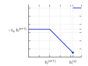
Figure 1: Plot of the loss function $L_{i,s}$. Notice that the loss in fact resembles a broken “V” .

In view of this proposition, we can replace the challenging problem of solving an optimization problem in $\mathbb{R}^{N}$ with solving the following simpler empirical risk minimization problem

$$\min_{r\in[0,1]}\sum_{i=1}^{n}\widetilde{L}(r,\mathbf{b}_{i})=\min_{r\in[0,1]}\sum_{i=1}^{n}\sum_{s=1}^{S}L_{s,i}(r,\widetilde{q}^{(s)},\widetilde{q}^{(s+1)}),$$ (6)

where $L_{s,i}(r,\widetilde{q}^{(s)}),\widetilde{q}^{(s+1)}):=-\frac{c_{s}}{e^{(s)}}(\widetilde{q}_{i}^{(s+1)}\mathds{1}_{\widetilde{q}_{i}^{(s+1)}\geq r}-r\mathds{1}_{\widetilde{q}_{i}^{(s+1)}<r\leq\widetilde{q}_{i}^{(s)}})$. In order to efficiently minimize this highly non-convex function, we draw upon the work of Mohri and Medina (2014) on minimization of sums of $v$-functions.

Definition 1.

A function $V\colon\mathbb{R}^{3}\to\mathbb{R}$ is a $v$-function if it admits the following form:

$$V(r,q_{1},q_{2})\\ \mspace{-4.0mu}=\mspace{-4.0mu}-a^{(1)}\mathds{1}_{r\leq q_{2}}-a^{(2)}r\mathds{1}_{q_{2}<r\leq q_{1}}+\Big{[}\frac{r}{\eta}-a^{(3)}\Big{]}\mathds{1}_{q_{1}<r<(1+\eta)q_{1}},$$

with $0\leq a^{(1)},a^{(2)},a^{(3)},\eta\leq\infty$ constants satisfying $a^{(1)}=a^{(2)}q_{2}$, $-a^{(2)}q_{1}\mathds{1}_{\eta>0}=\big{(}\frac{1}{\eta}q_{1}-a^{(3)}\big{)}\mathds{1}_{\eta>0}$. Under the convention that $0\cdot\infty=0$.

0:  Scores $(\widetilde{q}_{i}^{(s)})$, $1\leq n$, $1\leq s\leq S$.

1:  Define $(p_{is}^{(1)},p_{is}^{(2)})=(\widetilde{q}_{i}^{(s)},\widetilde{q}_{i}^{(s+1)})$; $m=nS$;

2:  $\mathcal{N}:=\bigcup_{i=1}^{n}\bigcup_{s=1}^{S}\{p_{is}^{(1)},p_{is}^{(2)}\}$;

3:  $(n_{1},...,n_{2m})={\bf Sort}(\mathcal{N})$;

4:  Set $\mathbf{d}_{i}:=(d_{1},d_{2})=\mathbf{0}$

5:  Set $d_{1}=-\sum_{i=1}^{n}\sum_{s=1}^{S}\frac{c_{s}}{e_{i}}p_{is}^{(2)}$;

6:  Set $r^{*}=-1$ and $L^{*}=\infty$

7:  for $j=2,\ldots,2m$ do

8:     if $n_{j-1}=p_{is}^{(2)}$ then

9:        $d_{1}=d_{1}+\frac{c_{s}}{e_{i}}p_{is}^{(2)}$; $\;d_{2}=d_{2}-\frac{c_{s}}{e_{i}};$

10:     else if $n_{j-1}=p_{is}^{(1)}$ then

11:        $d_{2}=d_{2}+\frac{c_{s}}{e_{s}}$

12:     end if

13:     $L=d_{1}-n_{j}d_{2}$;

14:     if $L<L^{*}$ then

15:        $L^{*}=L$; $r^{*}=n_{j}$;

16:     end if

17:  end for

18:  return  $r^{*}$;

Algorithm 1 Minimization algorithm

As suggested by their name, these functions admit a characteristic “V shape”. It is clear from Figure 1 that $L_{s,i}$ is a $v$-function with $a^{(1)}=\frac{c_{s}}{e^{(s)}}\widetilde{q}_{i}^{(s+1)}$, $a^{(2)}=\frac{c_{s}}{e^{(s)}}$ and $\eta=0$. Thus, we can apply the optimization algorithm given by Mohri and Medina (2014) to minimize (6) in $O(nS\log nS)$ time. Algorithm 1 gives the pseudocode of that the adaptation of this general algorithm to our problem. A proof of the correctness of this algorithm can be found in (Mohri and Medina, 2014).

We conclude this section by presenting learning guarantees for our algorithm. Our bounds are given in terms of the Rademacher complexity and the VC-dimension.

Definition 2.

Let $\mathcal{X}$ be a set and let $G:=\{g:\mathcal{X}\to\mathbb{R}\}$ be a family of functions. Given a sample $\mathcal{S}=(x_{1},\ldots,x_{n})\in\mathcal{X}$, the empirical Rademacher complexity of $G$ is defined by

$$\widehat{\mathfrak{R}}_{S}(G)=\frac{1}{n}\operatorname{\mathbb{E}}_{\sigma}\Big{[}\sup_{g\in G}\frac{1}{n}\sum_{i=1}^{n}\sigma_{i}g(x_{i})\Big{]},$$

where $\sigma_{i}$s are independent random variables distributed uniformly over the set $\{-1,1\}$.

Proposition 2.

Let $\mathfrak{m}=\min_{i}e_{i}>0$ and $\mathfrak{M}=\sum_{s=1}^{S}c_{s}$. Then, for any $\delta>0$, with probability at least $1-\delta$ over the draw of a sample $\mathcal{S}$ of size $n$, each of the following inequalities holds for all $r\in[0,1]$:

$$\operatorname{\mathbb{E}}[\widetilde{L}(r,\mathbf{b})] \leq\frac{1}{n}\sum_{i=1}^{n}\widetilde{L}(r,\mathbf{b}_{i})+C(\mathfrak{M},\mathfrak{m},n,\delta)$$ (7)

$$\frac{1}{n}\sum_{i=1}^{n}\widetilde{L}(r,\mathbf{b}_{i}) \leq\operatorname{\mathbb{E}}[\widetilde{L}(r,\mathbf{b})]+C(\mathfrak{M},\mathfrak{m},n,\delta),$$ (8)

where $C(\mathfrak{M},\mathfrak{m},n,\delta)=\frac{1}{\sqrt{n}}+\sqrt{\frac{\log(en)}{n}}+\sqrt{\frac{\mathfrak{M}\log(1/\delta)}{2\mathfrak{m}n}}$.

Proof.

Let $\Psi\colon S\mapsto\sup_{r\in[0,1]}\frac{1}{n}\sum_{i=1}^{n}\widetilde{L}(r,\mathbf{b}_{i})-\operatorname{\mathbb{E}}[\widetilde{L}(r,\mathbf{b})]$. Let $\mathcal{S}^{i}$ be a sample obtained from $\mathcal{S}$ by replacing $\mathbf{b}_{i}$ with $\mathbf{b}^{\prime}_{i}$. It is not hard to verify that $|\Psi(\mathcal{S})-\Psi(\mathcal{S}^{i})|\leq\frac{\mathfrak{M}}{n\mathfrak{m}}$. Thus, it follows from a standard learning bound that, with probability at least $1-\delta$,

$$\operatorname{\mathbb{E}}[\widetilde{L}(r,\mathbf{b})]\leq\frac{1}{n}\sum_{i=1}^{n}\widetilde{L}(r,\mathbf{b}_{i})+\widehat{\mathfrak{R}}_{S}(\mathcal{R})+\sqrt{\frac{\mathfrak{M}\log(1/\delta)}{2\mathfrak{m}n}},$$

where $\mathcal{R}=\{\overline{L}_{r}:\mathbf{b}\mapsto\widetilde{L}(r,\mathbf{b})|r\in[0,1]\}$. We proceed to bound the empirical Rademacher complexity of the class $\mathcal{R}$. For $q_{1}>q_{2}\geq 0$ let $\overline{L}(r,q_{1},q_{2})=q_{2}\mathds{1}_{q_{2}>r}+r\mathds{1}_{q_{1}\geq r\geq q_{2}}$. By definition of the Rademacher complexity we can write

$$\widehat{\mathfrak{R}}_{S}(\mathcal{R}) =\frac{1}{n}\operatorname{\mathbb{E}}_{\sigma}\Big{[}\sup_{r\in[0,1]}\sum_{i=1}^{n}\sigma_{i}\overline{L}_{r}(\mathbf{b}_{i})\Big{]}$$

$$=\frac{1}{n}\operatorname{\mathbb{E}}_{\sigma}\Big{[}\sup_{r\in[0,1]}\sum_{i=1}^{n}\sigma_{i}\sum_{s=1}^{S}\frac{c_{s}}{e_{s}}\overline{L}(r,\widetilde{q}_{i}^{(s)},\widetilde{q}_{i}^{(s+1)})\Big{]}$$

$$\leq\frac{1}{n}\operatorname{\mathbb{E}}_{\sigma}\Big{[}\sum_{s=1}^{S}\sup_{r\in[0,1]}\sum_{i=1}^{n}\sigma_{i}\psi_{s}(\overline{L}(r,\widetilde{q}_{i}^{(s)},\widetilde{q}_{i}^{(s+1)}))\Big{]},$$

where $\psi_{s}$ is the $\frac{c_{s}}{\mathfrak{m}}$-Lipschitz function mapping $x\mapsto\frac{c_{s}}{e^{(s)}}x$. Therefore, by Talagrand’s contraction lemma (Ledoux and Talagrand, 2011), the last term is bounded by

$$\sum_{s=1}^{S}\frac{c_{s}}{n\mathfrak{m}}\operatorname{\mathbb{E}}_{\sigma}\!\sup_{r\in[0,1]}\sum_{i=1}^{n}\sigma_{i}\overline{L}(r,\widetilde{q}_{i}^{(s)},\widetilde{q}_{i}^{(s+1)})\!=\!\sum_{s=1}^{S}\frac{c_{s}}{\mathfrak{m}}\widehat{\mathfrak{R}}_{\mathcal{S}_{s}}(\widetilde{\mathcal{R}}),$$

where $\mathcal{S}_{s}=\big{(}(\widetilde{q}_{1}^{(s)},\widetilde{q}_{1}^{(s+1)}),\ldots,(\widetilde{q}_{n}^{(s)},\widetilde{q}_{n}^{(s+1)})\big{)}$ and $\widetilde{\mathcal{R}}:=\{\overline{L}(r,\cdot,\cdot)|r\in[0,1]\}$. The loss $\overline{L}(r,\widetilde{q}^{(s)},\widetilde{q}^{(s+1)})$ in fact evaluates to the negative revenue of a second-price auction with highest bid $\widetilde{q}^{(s)}$ and second highest bid $\widetilde{q}^{(s+1)}$ (Mohri and Medina, 2014). Therefore, by Propositions 9 and 10 of Mohri and Medina (2014) we can write

$$\widehat{\mathfrak{R}}_{\mathcal{S}_{s}}(\widetilde{\mathcal{R}}) \leq\frac{1}{n}\operatorname{\mathbb{E}}_{\sigma}\Big{[}\sup_{r\in[0,1]}\sum_{i=1}^{n}r\sigma_{i}\Big{]}+\sqrt{\frac{2\log en}{n}}$$

$$\leq\Big{(}\frac{1}{\sqrt{n}}+\sqrt{\frac{2\log en}{n}}\Big{)},$$

which concludes the proof. ∎

Corollary 1.

Under the hypotheses of Proposition 2, let $\widehat{r}$ denote the empirical minimizer and $r^{*}$ the minimizer of the expected loss. Then, for any $\delta>0$, with probability at least $1-\delta$, the following inequality holds:

$$\operatorname{\mathbb{E}}[\widetilde{L}(\widehat{r},\mathbf{b})]-\operatorname{\mathbb{E}}[\widetilde{L}(r^{*},\mathbf{b})]\\ \leq 2C\Big{(}\mathfrak{M},\mathfrak{m},n,\frac{\delta}{2}\Big{)}.$$

Proof.

By the union bound, (7) and (8) hold simultaneously with probability at least $1-\delta$ if $\delta$ is replaced by $\delta/2$ in those expression. Adding both inequalities and using the fact that $\widehat{r}$ is an empirical minimizer yields the result. ∎

It is worth noting that our algorithm is well defined whether or not the buyers bid in equilibrium. Indeed, the algorithm consists of the minimization over $r$ of an observable quantity. While we can guarantee convergence to a solution of (1) only when buyers play a symmetric BNE, our algorithm will still find an approximate solution to

$$\min_{r\in[0,1]}\operatorname{\mathbb{E}}_{\mathbf{b}}[L(r,\mathbf{b})],$$

which remains a quantity of interest that can be close to (1) if buyers are close to the equilibrium.

5 CONVERGENCE OF EMPIRICAL EQUILIBRIA

A crucial assumption in the study of GSP auctions, including this work, is that advertisers bid in a Bayes-Nash equilibrium (Lucier et al., 2012; Sun et al., 2014). This assumption is partially justified by the fact that advertisers can infer the underlying distribution $F$ using as observations the outcomes of the past repeated auctions and can thereby implement an efficient equilibrium.

In this section, we provide a stronger theoretical justification in support of this assumption: we quantify the difference between the bidding function calculated using observed empirical distributions and the true symmetric bidding function in equilibria. For the sake of notation simplicity, we will consider only the rank-by-bid GSP auction.

Let $\mathcal{S}_{v}=(v_{1},\ldots,v_{n})$ be an i.i.d. sample of values drawn from a continuous distribution $F$ with density function $f$. Assume without loss of generality that $v_{1}\leq\ldots\leq v_{n}$ and let $\mathbf{v}$ denote the vector defined by $\mathbf{v}_{i}=v_{i}$. Let $\widehat{F}$ denote the empirical distribution function induced by $\mathcal{S}_{v}$ and let $\mathbf{F}\in\mathbb{R}^{n}$ and $\mathbf{G}\in\mathbb{R}^{n}$ be defined by $\mathbf{F}_{i}=\widehat{F}(v_{i})=i/n$ and $\mathbf{G}_{i}=1-\mathbf{F}_{i}$.

We consider a discrete GSP auction where the advertiser’s valuations are i.i.d. samples drawn from a distribution $\widehat{F}$. In the event where two or more advertisers admit the same valuation, ties are broken randomly. Denote by $\widehat{\beta}$ the bidding function for this auction in equilibrium (when it exists). We are interested in characterizing $\widehat{\beta}$ and in providing guarantees on the convergence of $\widehat{\beta}$ to $\beta$ as the sample size increases.

We first introduce the notation used throughout this section.

Definition 3.

Given a vector $\mathbf{F}\in\mathbb{R}^{n}$, the backwards difference operator $\Delta:\mathbb{R}^{n}\to\mathbb{R}^{n}$ is defined as:

$$\Delta\mathbf{F}_{i}=\mathbf{F}_{i}-\mathbf{F}_{i-1},$$

for $i>1$ and $\Delta\mathbf{F}_{1}=\mathbf{F}_{1}$.

We will denote $\Delta\Delta\mathbf{F}_{i}$ by $\Delta^{2}\mathbf{F}_{i}$. Given any $k\in\mathbb{N}$ and a vector $\mathbf{F}$, the vector $\mathbf{F}^{k}$ is defined as $\mathbf{F}^{k}_{i}=(\mathbf{F}_{i})^{k}$. Let us now define the discrete analog of the function $z_{s}$ that quantifies the probability of winning slot $s$.

Proposition 3.

In a symmetric efficient equilibrium of the discrete GSP, the probability $\widehat{z}_{s}(v)$ that an advertiser with valuation $v$ is assigned to slot $s$ is given by

$$\widehat{z}_{s}(v)\\ =\sum_{j=0}^{N-s}\sum_{k=0}^{s-1}\binom{N-1}{j,k,N\!-\!1\!-\!j\!-\!k}\frac{\mathbf{F}_{i-1}^{j}\mathbf{G}_{i}^{k}}{(N-j-k)n^{N-1-j-k}},$$

if $v=v_{i}$ and otherwise by

$$\widehat{z}_{s}(v)=\binom{N-1}{s-1}\lim_{v^{\prime}\rightarrow v^{-}}\widehat{F}(v^{\prime})^{p}(1-\widehat{F}(v))^{s-1}=:\widehat{z}_{s}^{-}(v),$$

where $p=N-s$.

In particular, notice that $\widehat{z}_{s}^{-}(v_{i})$ admits the simple expression

$$\widehat{z}_{s}^{-}(v_{i})=\binom{N-1}{s-1}\mathbf{F}_{i-1}^{p}\mathbf{G}_{i-1}^{s-1},$$

which is the discrete version of the function $z_{s}$. On the other hand, even though $\widehat{z}_{s}(v_{i})$ does not admit a closed-form, it is not hard to show that

$$\widehat{z}_{s}(v_{i})=\binom{N-1}{s-1}\mathbf{F}_{i-1}^{p}\mathbf{G}_{i}^{s-1}+O\Big{(}\frac{1}{n}\Big{)}.$$ (9)

Which again can be thought of as a discrete version of $z_{s}$. The proof of this and all other propositions in this section are deferred to the Appendix. Let us now define the lower triangular matrix $\mathbf{M}(s)$ by:

$$\mathbf{M}_{ij}(s)=-\binom{N-1}{s-1}\frac{n\Delta\mathbf{F}_{j}^{p}\Delta\mathbf{G}_{i}^{s}}{s},$$

for $i>j$ and

$$\mathbf{M}_{ii}(s)=\!\!\sum_{j=0}^{N-s-1}\sum_{k=0}^{s-1}\binom{N-1}{j,k,N\!-\!1\!-\!j\!-\!k}\tfrac{\mathbf{F}_{i-1}^{j}\mathbf{G}_{i}^{k}}{(N\!-\!j\!-\!k)n^{N\!-\!1\!-\!j\!-\!k}}.$$

Proposition 4.

If the discrete GSP auction admits a symmetric efficient equilibrium, then its bidding function $\widehat{\beta}$ satisfies $\widehat{\beta}(v_{i})=\boldsymbol{\beta}_{i}$, where $\boldsymbol{\beta}$ is the solution of the following linear equation.

$$\mathbf{M}\boldsymbol{\beta}=\mathbf{u},$$ (10)

with $\mathbf{M}=\sum_{s=1}^{S}c_{s}\mathbf{M}(s)$ and $\mathbf{u}_{i}=\sum_{s=1}^{S}\Big{(}c_{s}z_{s}(v_{i})v_{i}-\sum_{j=1}^{i}\widehat{z}_{s}^{-}(v_{j})\Delta\mathbf{v}_{j}\Big{)}$.

To gain some insight about the relationship between $\widehat{\beta}$ and $\beta$, we compare equations (10) and (2). An integration by parts of the right-hand side of (2) and the change of variable $G(v)=1-F(v)$ show that $\beta$ satisfies

$$\sum_{s=1}^{S}c_{s}vz_{s}(v)-\int_{0}^{v}\frac{dz_{s}(t)}{dt}tdt\\ =\sum_{s=1}^{S}c_{s}\binom{N-1}{s-1}G(v)^{s-1}\int_{0}^{v}\beta(t)dF^{p}.$$ (11)

On the other hand, equation (10) implies that for all $i$

$$\mathbf{u}_{i}=\sum_{s=1}^{S}c_{s}\bigg{[}\mathbf{M}_{ii}(s)\boldsymbol{\beta}_{i}-\binom{N-1}{s-1}\frac{n\Delta\mathbf{G}_{i}^{s}}{s}\sum_{j=1}^{i-1}\Delta\mathbf{F}_{j}^{p}\boldsymbol{\beta}_{j}\bigg{]}.$$ (12)

Moreover, by Lemma 2 and Proposition 10 in the Appendix, the equalities $-\frac{n\Delta\mathbf{G}_{i}^{s}}{s}=\mathbf{G}_{i}^{s-1}+O\big{(}\frac{1}{n}\big{)}$ and

$$\mathbf{M}_{ii}(s)=\frac{1}{2n}\binom{N-1}{s-1}p\mathbf{F}^{p-1}_{i-1}\mathbf{G}_{i}^{s-1}+O\Big{(}\frac{1}{n^{2}}\Big{)},$$

hold. Thus, equation (12) resembles a numerical scheme for solving (11) where the integral on the right-hand side is approximated by the trapezoidal rule. Equation (11) is in fact a Volterra equation of the first kind with kernel

$$K(t,v)=\sum_{s=1}^{S}\binom{N-1}{s-1}G(v)^{s-1}pF^{p-1}(t).$$

Therefore, we could benefit from the extensive literature on the convergence analysis of numerical schemes for this type of equations (Baker, 1977; Kress et al., 1989; Linz, 1985). However, equations of the first kind are in general ill-posed problems (Kress et al., 1989), that is small perturbations on the equation can produce large errors on the solution. When the kernel $K$ satisfies $\min_{t\in[0,1]}K(t,t)>0$, there exists a standard technique to transform an equation of the first kind to an equation of the second kind, which is a well posed problem. Thus, making the convergence analysis for these types of problems much simpler. The kernel function appearing in (11) does not satisfy this property and therefore these results are not applicable to our scenario. To the best of our knowledge, there exists no quadrature method for solving Volterra equations of the first kind with vanishing kernel.

In addition to dealing with an uncommon integral equation, we need to address the problem that the elements of (10) are not exact evaluations of the functions defining (11) but rather stochastic approximations of these functions. Finally, the grid points used for the numerical approximation are also random.

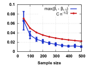
Figure 2: (a) Empirical verification of Assumption 2. The blue line corresponds to the quantity $\max_{i}\Delta\boldsymbol{\beta}_{i}$. In red we plot the desired upper bound for $C=1/2$.

In order to prove convergence of the function $\widehat{\beta}$ to $\beta$ we will make the following assumptions

Assumption 1.

There exists a constant $c>0$ such that $f(x)>c$ for all $x\in[0,1]$.

This assumption is needed to ensure that the difference between consecutive samples $v_{i}-v_{i-1}$ goes to $0$ as $n\rightarrow\infty$, which is a necessary condition for the convergence of any numerical scheme.

Assumption 2.

The solution $\boldsymbol{\beta}$ of (10) satisfies $v_{i},\boldsymbol{\beta}_{i}\geq 0$ for all $i$ and $\max_{i\in 1,\ldots,n}\Delta\boldsymbol{\beta}_{i}\leq\frac{C}{\sqrt{n}}$, for some universal constant $C$.

Since $\boldsymbol{\beta}_{i}$ is a bidding strategy in equilibrium, it is reasonable to expect that $v_{i}\geq\boldsymbol{\beta}_{i}\geq 0$. On the other hand, the assumption on $\Delta\boldsymbol{\beta}_{i}$ is related to the smoothness of the solution. If the function $\beta$ is smooth, we should expect the approximation $\widehat{\beta}$ to be smooth too. Both assumptions can in practice be verified empirically, Figure 2 depicts the quantity $\max_{i\in 1,\ldots,n}\Delta\boldsymbol{\beta}_{i}$ as a function of the sample size $n$.

Assumption 3.

The solution $\beta$ to (2) is twice continuously differentiable.

This is satisfied if for instance the distribution function $F$ is twice continuously differentiable. We can now present our main result.

Theorem 3.

If Assumptions 1, 2 and 3 are satisfied, then, for any $\delta>0$, with probability at least $1-\delta$ over the draw of a sample of size $n$, the following bound holds for all $i\in[1,n]$:

$$|\widehat{\beta}(v_{i})-\beta(v_{i})|\leq e^{C}\bigg{[}\frac{\log(\frac{2}{\delta})^{\frac{N}{2}}}{\sqrt{n}}q\Big{(}n,\frac{2}{\delta}\Big{)}^{3}+\frac{Cq(n,\frac{2}{\delta})}{n^{3/2}}\bigg{]}.$$

where $q(n,\delta)=\frac{2}{c}\log(nc/2\delta)$ with $c$ defined in Assumption 1, and where $C$ is a universal constant.

The proof of this theorem is highly technical, thus, we defer it to Appendix F.

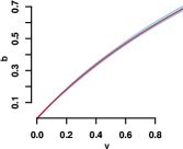
Figure 3: Approximation of the empirical bidding function $\widehat{\beta}$ to the true solution $\beta$. The true solution is shown in red and the shaded region represents the confidence interval of $\widehat{\beta}$ when simulating the discrete $GSP$ 10 times with a sample of size $200$. Where $N=3$, $S=2$, $c_{1}=1$, $c_{2}=0.5$ and bids were sampled uniformly from $[0,1]$

6 EXPERIMENTS

Here we present preliminary experiments showing the advantages of our algorithm. We also present empirical evidence showing that the procedure proposed in Sun et al. (2014) to estimate valuations from bids is incorrect. In contrast, our density estimation algorithm correctly recovers valuations from bids in equilibrium.

6.1 SETUP

Let $F_{1}$ and $F_{2}$ denote the distributions of two truncated log-normal random variables with parameters $\mu_{1}=\log(.5)$, $\sigma_{1}=.8$ and $\mu_{2}=\log(2)$, $\sigma=.1$; the mixture parameter was set to $1/2$ . Here, $F_{1}$ is truncated to have support in $[0,1.5]$ and the support of $F_{2}=[0,2.5]$. We consider a GSP with $N=4$ advertisers with $S=3$ slots and position factors $c_{1}=1$, $c_{2}=,45$ and $c_{3}=1$. Based on the results of Section 5 we estimate the bidding function $\beta$ with a sample of 2000 points and we show its plot in Figure 4.

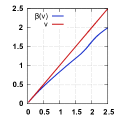
Figure 4: Bidding function for our experiments in blue and identity function in red.

We proceed to evaluate the method proposed by Sun et al. (2014) for recovering advertisers valuations from bids in equilibrium. The assumption made by the authors is that the advertisers play a SNE in which case valuations can be inferred by solving a simple system of inequalities defining the SNE (Varian, 2007). Since the authors do not specify which SNE the advertisers are playing we select the one that solves the SNE conditions with equality.

We generated a sample $\mathcal{S}$ consisting of $n=300$ i.i.d. outcomes of our simulated auction. Since $N=4$, the effective size of this sample is of $1200$ points. We generated the outcome bid vectors $\mathbf{b}_{i},\ldots,\mathbf{b}_{n}$ by using the equilibrium bidding function $\beta$. Assuming that the bids constitute a SNE we estimated the valuations and Figure 5 shows an histogram of the original sample as well as the histogram of the estimated valuations. It is clear from this figure that this procedure does not accurately recover the distribution of the valuations. By contrast, the histogram of the estimated valuations using our density estimation algorithm is shown in Figure 5(c). The kernel function used by our algorithm was a triangular kernel given by $K(u)=(1-|u|)\mathds{1}_{|u|\leq 1}$. Following the experimental setup of Guerre et al. (2000) the bandwidth $h$ was set to $h=1.06\widehat{\sigma}n^{1/5}$, where $\widehat{\sigma}$ denotes the standard deviation of the sample of bids.

Finally, we use both our density estimation algorithm and discriminative learning algorithm to infer the optimal value of $r$. To test our algorithm we generated a test sample of size $n=500$ with the procedure previously described. The results are shown in Table 1.

Density estimation	Discriminative
1.42 $\pm$ 0.02	1.85 $\pm$ 0.02

Table 1: Mean revenue for our two algorithms.

(a)

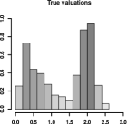
(b)

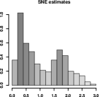
(c)

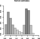
Figure 5: Comparison of methods for estimating valuations from bids. (a) Histogram of true valuations. (b) Valuations estimated under the SNE assumption. (c) Density estimation algorithm.

7 CONCLUSION

We proposed and analyzed two algorithms for learning optimal reserve prices for generalized second price auctions. Our first algorithm is based on density estimation and therefore suffers from the standard problems associated with this family of algorithms. Furthermore, this algorithm is only well defined when bidders play in equilibrium. Our second algorithm is novel and is based on learning theory guarantees. We show that the algorithm admits an efficient $O(nS\log(nS))$ implementation. Furthermore, our theoretical guarantees are more favorable than those presented for the previous algorithm of Sun et al. (2014). Moreover, even though it is necessary for advertisers to play in equilibrium for our algorithm to converge to optimality, when bidders do not play an equilibrium, our algorithm is still well defined and minimizes a quantity of interest albeit over a smaller set. We also presented preliminary experimental results showing the advantages of our algorithm. To our knowledge, this is the first attempt to apply learning algorithms to the problem of reserve price selection in GSP auctions. We believe that the use of learning algorithms in revenue optimization is crucial and that this work may preface a rich research agenda including extensions of this work to a general learning setup where auctions and advertisers are represented by features. Additionally, in our analysis, we considered two different ranking rules. It would be interesting to combine the algorithm of Zhu et al. (2009) with this work to learn both a ranking rule and an optimal reserve price. Finally, we provided the first analysis of convergence of bidding functions in an empirical equilibrium to the true bidding function. This result on its own is of great importance as it justifies the common assumption of advertisers playing in a Bayes-Nash equilibrium.

Appendix A THE ENVELOPE THEOREM

The envelope theorem is a well known result in auction mechanism design characterizing the maximum of a parametrized family of functions. The most general form of this theorem is due to Milgrom and Segal (2002) and we include its proof here for completeness. We will let $X$ be an arbitrary space will consider a function $f\colon X\times[0,1]\to\mathbb{R}$ we define the envelope function $V$ and the set valued function $X^{*}$ as

$$V(t) =\sup_{x\in X}f(x,t)\qquad\text{and}$$

$$X^{*}(t) =\{x\in X|f(x,t)=V(t)\}.$$

We show a plot of the envelope function in figure 6.

Theorem 4 (Envelope Theorem).

Let $f$ be an absolutely continuous function for every $x\in X$. Suppose also that there exists an integrable function $b\colon[0,1]\to\mathbb{R}_{+}$ such that for every $x\in X$, $\frac{df}{dt}(x,t)\leq b(t)$ almost everywhere in $t$. Then $V$ is absolutely continuous. If in addition $f(x,\cdot)$ is differentiable for all $x\in X$, $X^{*}(t)\neq\emptyset$ almost everywhere on $[0,1]$ and $x^{*}(t)$ denotes an arbitrary element in $X^{*}(t)$, then

$$V(t)=V(0)+\int_{0}^{t}\frac{df}{dt}(x^{*}(s),s)ds.$$

Proof.

By definition of $V$, for any $t^{\prime},t^{\prime\prime}\in[0,1]$ we have

$$|V(t^{\prime\prime})-V(t^{\prime})| \leq\sup_{x\in X}|f(x,t^{\prime\prime})-f(x,t^{\prime})|$$

$$=\sup_{x\in X}\Big{|}\int_{t^{\prime}}^{t^{\prime\prime}}\frac{df}{dt}(x,s)\Big{|}\leq\int_{t^{\prime}}^{t^{\prime\prime}}b(t)dt.$$

This easily implies that $V(t)$ is absolutely continuous. Therefore, $V$ is differentiable almost everywhere and $V(t)=V(0)+\int_{0}^{t}V^{\prime}(s)ds$. Finally, if $f(x,t)$ is differentiable in $t$ then we know that $V^{\prime}(t)=\frac{df}{dt}(x^{*}(t),t)$ for any $x^{*}(t)\in X^{*}(t)$ whenever $V^{\prime}(t)$ exists and the result follows. ∎

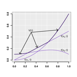
Figure 6: Illustration of the envelope function.

Appendix B ELEMENTARY CALCULATIONS

We present elementary results of Calculus that will be used throughout the rest of this Appendix.

Lemma 2.

The following equality holds for any $k\in\mathbb{N}$:

$$\Delta\mathbf{F}_{i}^{k}=\frac{k}{n}\mathbf{F}_{i-1}^{k-1}+\frac{i^{k-2}}{n^{k-2}}O\Big{(}\frac{1}{n^{2}}\Big{)},$$

and

$$\Delta\mathbf{G}_{i}^{k}=-\frac{k}{n}\mathbf{G}_{i-1}^{k-1}+O\Big{(}\frac{1}{n^{2}}\Big{)}.$$

Proof.

The result follows from a straightforward application of Taylor’s theorem to the function $h(x)=x^{k}$. Notice that $\mathbf{F}^{k}_{i}=h(i/n)$, therefore:

$$\Delta\mathbf{F}_{i}^{k} =h\Big{(}\frac{i-1}{n}+\frac{1}{n}\Big{)}-h\Big{(}\frac{i-1}{n}\Big{)}$$

$$=h^{\prime}\Big{(}\frac{i-1}{n}\Big{)}\frac{1}{n}+h^{\prime\prime}(\zeta_{i})\frac{1}{2n^{2}}$$

$$=\frac{k}{n}\mathbf{F}_{i-1}^{k-1}+h^{\prime\prime}(\zeta_{i})\frac{1}{2n^{2}},$$

for some $\zeta_{i}\in[(i-1)/n,i/n]$. Since $h^{\prime\prime}(x)=k(k-1)x^{k-2}$, it follows that the last term in the previous expression is in $(i/n)^{k-2}O(1/n^{2})$. The second equality can be similarly proved. ∎

Proposition 5.

Let $a,b\in\mathbb{R}$ and $N\geq 1$ be an integer, then

$$\sum_{j=0}^{N}\binom{N}{j}\frac{a^{j}b^{N-j}}{j+1}=\frac{(a+b)^{N+1}-b^{N+1}}{a(N+1)}$$ (13)

Proof.

The proof relies on the fact that $\frac{a^{j}}{j+1}=\frac{1}{a}\int_{0}^{a}t^{j}dt$. The left hand side of (13) is then equal to

$$\frac{1}{a}\int_{0}^{a}\sum_{j=0}^{N}\binom{N}{j}t^{j}b^{N-j}dt =\frac{1}{a}\int_{0}^{a}(t+b)^{N}dt$$

$$=\frac{(a+b)^{N+1}-b^{N+1}}{a(N+1)}.$$

∎

Lemma 3.

If the sequence $a_{i}\geq 0$ satisfies

$$a_{i}\leq\delta \quad\forall i\leq r$$

$$a_{i}\leq A+B\sum_{j=1}^{i-1}a_{j} \quad\forall i>r.$$

Then $a_{i}\leq(A+r\delta B)(1+B)^{i-r-1}\leq(A+r\delta B)e^{B(i-r-1)}\;\forall i>r$.

This lemma is well known in the numerical analysis community and we include the proof here for completeness.

Proof.

We proceed by induction on $i$. The base of our induction is given by $i=r+1$ and it can be trivially verified. Indeed, by assumption

$$a_{r+1}\leq A+r\delta B.$$

Let us assume that the proposition holds for values less than $i$ and let us try to show it also holds for $i$.

$$a_{i} \leq A+B\sum_{j=1}^{r}a_{j}+B\sum_{j=r+1}^{i-1}a_{j}$$

$$\leq A+rB\delta+B\sum_{j=r+1}^{i-1}(A+rB\delta)(1+B)^{j-r-1}$$

$$=A+rB\delta+(A+rB\delta)B\sum_{j=0}^{i-r-2}(1+B)^{j}$$

$$=A+rB\delta+(A+rB\delta)B\frac{(1+B)^{i-r-1}-1}{B}$$

$$=(A+rB\delta)(1+B)^{i-r-1}.$$

∎

Lemma 4.

Let $W_{0}\colon[e,\infty)\to\mathbb{R}$ denote the main branch of the Lambert function, i.e. $W_{0}(x)e^{W_{0}(x)}=x$. The following inequality holds for every $x\in[e,\infty)$.

$$\log(x)\geq W_{0}(x).$$

By definition of $W_{0}$ we see that $W_{0}(e)=1$. Moreover, $W_{0}$ is an increasing function. Therefore for any $x\in[e,\infty)$

$$W_{0}(x)\geq 1$$

$$\Rightarrow W_{0}(x)x\geq x$$

$$\Rightarrow W_{0}(x)x\geq W_{0}(x)e^{W_{0}(x)}$$

$$\Rightarrow x\geq e^{W_{0}(x)}.$$

The result follows by taking logarithms on both sides of the last inequality.

Appendix C PROOF OF PROPOSITION 4

Here, we derive the linear equation that must be satisfied by the bidding function $\widehat{\beta}$. For the most part, we adapt the analysis of Gomes and Sweeney (2014) to a discrete setting.

Proposition 3.

In a symmetric efficient equilibrium of the discrete GSP, the probability $\widehat{z}_{s}(v)$ that an advertiser with valuation $v$ is assigned to slot $s$ is given by

$$\widehat{z}_{s}(v)\\ =\sum_{j=0}^{N-s}\sum_{k=0}^{s-1}\binom{N-1}{j,k,N\!-\!1\!-\!j\!-\!k}\frac{\mathbf{F}_{i-1}^{j}\mathbf{G}_{i}^{k}}{(N-j-k)n^{N-1-j-k}},$$

if $v=v_{i}$ and otherwise by

$$\widehat{z}_{s}(v)=\binom{N-1}{s-1}\lim_{v^{\prime}\rightarrow v^{-}}\widehat{F}(v^{\prime})^{p}(1-\widehat{F}(v))^{s-1}=:\widehat{z}_{s}^{-}(v),$$

where $p=N-s$.

Proof.

Since advertisers play an efficient equilibrium, these probabilities depend only on the advertisers’ valuations. Let $A_{j,k}(s,v)$ denote the event that $j$ buyers have a valuation lower than $v$, $k$ of them have a valuation higher than $v$ and $N-1-j-k$ a valuation exactly equal to $v$. Then, the probability of assigning $s$ to an advertiser with value $v$ is given by

$$\sum_{j=0}^{N-s}\sum_{k=0}^{s-1}\frac{1}{N-i-j}\Pr(A_{j,k}(s,v)).$$ (14)

The factor $\frac{1}{N-i-j}$ appears due to the fact that the slot is randomly assigned in the case of a tie. When $v=v_{i}$, this probability is easily seen to be:

$$\binom{N-1}{j,k,N\!-\!1\!-\!j\!-\!k}\frac{\mathbf{F}_{i-1}^{j}\mathbf{G}_{i}^{k}}{n^{N-1-j-k}}.$$

On the other hand, if $v\in(v_{i-1},v_{i})$ the event $A_{j,k}(s,v)$ happens with probability zero unless $j=N-s$ and $k=s-1$. Therefore, (14) simplifies to

$$\binom{N\!-\!1}{s\!-\!1}\widehat{F}(v)^{p}(1-\widehat{F}(v))^{s-1}\\ =\binom{N\!-\!1}{s\!-\!1}\lim_{v^{\prime}\rightarrow v^{-}}\widehat{F}(v^{\prime})^{p}(1-\widehat{F}(v))^{s-1}.$$

∎

Proposition 6.

Let $\operatorname{\mathbb{E}}[P^{PE}(v)]$ denote the expected payoff of an advertiser with value $v$ at equilibrium. Then

$$\operatorname{\mathbb{E}}[P^{PE}(v_{i})]=\sum_{s=1}^{S}c_{s}\Big{[}\widehat{z}_{s}(v_{i})v_{i}-\sum_{j=1}\widehat{z}_{s}^{-}(v_{i})(v_{i}-v_{i-1})\Big{]}.$$

Proof.

By the revelation principle (Gibbons, 1992), there exists a truth revealing mechanism with the same expected payoff function as the GSP with bidders playing an equilibrium. For this mechanism, we then must have

$$v\in\arg\!\max_{\overline{v}\in[0,1]}\sum_{s=1}^{S}c_{s}\widehat{z}_{s}(\overline{v})v-\operatorname{\mathbb{E}}[P^{PE}(v)].$$

By the envelope theorem (see Theorem 4), we have

$$\sum_{s=1}^{S}c_{s}\widehat{z}_{s}(v_{i})v_{i}-\operatorname{\mathbb{E}}[P^{PE}(v_{i})]=-\operatorname{\mathbb{E}}[P^{PE}(0)]+\sum_{s=1}^{S}\int_{0}^{v_{i}}\widehat{z}_{s}(t)dt.$$

Since the expected payoff of an advertiser with valuation $0$ should be zero too, we see that

$$\operatorname{\mathbb{E}}[P^{PE}(v_{i})]=c_{s}\widehat{z}_{s}(v_{i})v_{i}-\int_{0}^{v_{i}}\widehat{z}_{s}(t)dt.$$

Using the fact that $\widehat{z}_{s}(t)\equiv\widehat{z}^{-}_{s}(v_{i})$ for $t\in(v_{i-1},v_{i})$ we obtain the desired expression. ∎

Proposition 4.

If the discrete GSP auction admits a symmetric efficient equilibrium, then its bidding function $\widehat{\beta}$ satisfies $\widehat{\beta}(v_{i})=\boldsymbol{\beta}_{i}$, where $\boldsymbol{\beta}$ is the solution of the following linear equation:

$$\mathbf{M}\boldsymbol{\beta}=\mathbf{u}.$$

where $\mathbf{M}=\sum_{s=1}^{S}c_{s}\mathbf{M}(s)$ and

$$\mathbf{u}_{i}=\sum_{s=1}^{S}\Big{(}c_{s}z_{s}(v_{i})v_{i}-\sum_{j=1}^{i}\widehat{z}_{s}^{-}(v_{j})\Delta\mathbf{v}_{j}\Big{)}.$$

Proof.

Let $\operatorname{\mathbb{E}}[P^{\widehat{\beta}}(v_{i})]$ denote the expected payoff of an advertiser with value $v_{i}$ when all advertisers play the bidding function $\widehat{\beta}$. Let $A(s,v_{i},v_{j})$ denote the event that an advertiser with value $v_{i}$ gets assigned slot $s$ and the $s$-th highest valuation among the remaining $N-1$ advertisers is $v_{j}$. If the event $A(s,v_{i},v_{j})$ takes place, then the advertiser has a expected payoff of $c_{s}\beta(v_{j})$. Thus,

$$\operatorname{\mathbb{E}}[P^{\beta}(v_{i})]=\sum_{s=1}^{S}c_{s}\sum_{j=1}^{i}\beta(v_{j})\Pr(A(s,v_{i},v_{j})).$$

In order for event $A(s,v_{i},v_{j})$ to occur for $i\neq j$, $N-s$ advertisers must have valuations less than or equal to $v_{j}$ with equality holding for at least one advertiser. Also, the valuation of $s-1$ advertisers must be greater than or equal to $v_{i}$. Keeping in mind that a slot is assigned randomly in the event of a tie, we see that $A(s,v_{i},v_{j})$ occurs with probability

$$\sum_{l=0}^{N-s-1}\sum_{k=0}^{s-1}\binom{N\!-\!1}{s\!-\!1}\binom{s\!-\!1}{k}\binom{N\!-\!s}{l}\frac{\mathbf{F}_{j-1}^{l}}{n^{N-s-l}}\frac{\mathbf{G}_{i}^{s-1-k}}{(k+1)n^{k}}$$

$$=\binom{N\!-\!1}{s\!-\!1}\sum_{l=0}^{N-s-1}\binom{N\!-\!s}{l}\frac{\mathbf{F}_{j-1}^{l}}{n^{N-s-l}}\sum_{k=0}^{s-1}\binom{s\!-\!1}{k}\frac{\mathbf{G}_{i}^{s-1-k}}{(k+1)n^{k}}$$

$$=\binom{N\!-\!1}{s\!-\!1}\Big{(}\big{(}\mathbf{F}_{j-1}+\frac{1}{n}\big{)}^{N-s}-F_{j-1}^{N-s}\Big{)}\Big{(}\frac{n\big{(}\mathbf{G}_{i-1}^{s}-\mathbf{G}_{i}^{s}\big{)}}{s}\Big{)}$$

$$=-\binom{N-1}{s-1}\frac{n\Delta\mathbf{F}_{j}\Delta\mathbf{G}_{i}}{s},$$

where the second equality follows from an application of the binomial theorem and Proposition 5. On the other hand if $i=j$ this probability is given by:

$$\sum_{j=0}^{N-s-1}\sum_{k=0}^{s-1}\binom{N-1}{j,k,N-1-j-k}\frac{\mathbf{F}_{i-1}^{j}\mathbf{G}_{i}^{k}}{(N-j-k)n^{N-1-j-k}}$$

It is now clear that $\mathbf{M}(s)_{i,j}=\Pr(A(s,v_{i},v_{j}))$ for $i\geq j$. Finally, given that in equilibrium the equality $\operatorname{\mathbb{E}}[P^{PE}(v)]=\operatorname{\mathbb{E}}[P^{\widehat{\beta}}(v)]$ must hold, by Proposition 6, we see that $\boldsymbol{\beta}$ must satisfy equation (10). ∎

We conclude this section with a simpler expression for $\mathbf{M}_{ii}(s)$. By adding and subtracting the term $j=N-s$ in the expression defining $\mathbf{M}_{ii}(s)$ we obtain

$$\mathbf{M}_{ii}(s) =\widehat{z}_{s}(v_{i})-\sum_{k=0}^{s-1}\binom{N\!-\!1}{N\!-\!s,k,s\!-\!1\!-\!k}\frac{\mathbf{F}_{i-1}^{p}\mathbf{G}_{i}^{k}}{(s-k)n^{s-1-k}}$$

$$=\widehat{z}_{s}(v_{i})-\binom{N-1}{s-1}\sum_{k=1}^{s-1}\binom{s-1}{k}\frac{\mathbf{F}_{i-1}^{p}\mathbf{G}_{i}^{k}}{(s-k)n^{s-1-k}}$$

$$=\widehat{z}_{s}(v_{i})+\binom{N-1}{s-1}\mathbf{F}_{i-1}^{p}\frac{n\Delta\mathbf{G}_{i}}{s},$$ (15)

where again we used Proposition 5 for the last equality.

Appendix D HIGH PROBABILITY BOUNDS

In order to improve the readability of our proofs we use a fixed variable $C$ to refer to a universal constant even though this constant may be different in different lines of a proof.

Theorem 5.

(Glivenko-Cantelli Theorem) Let $v_{1},\ldots,v_{n}$ be an i.i.d. sample drawn from a distribution $F$. If $\widehat{F}$ denotes the empirical distribution function induced by this sample, then with probability at least $1-\delta$ for all $v\in\mathbb{R}$

$$|\widehat{F}(v)-F(v)|\leq C\sqrt{\frac{\log(1/\delta)}{n}}.$$

Proposition 7.

Let $X_{1},\ldots,X_{n}$ be an $i.i.d$ sample from a distribution $F$ supported in $[0,1]$. Suppose $F$ admits a density $f$ and assume $f(x)>c$ for all $x\in[0,1]$. If $X^{(1)},\ldots,X^{(n)}$ denote the order statistics of a sample of size $n$ and we let $X^{(0)}=0$, then

$$\Pr(\max_{i\in\{1,\ldots,n\}}X^{(i)}-X^{(i-1)}>\epsilon)\leq\frac{3}{\epsilon}e^{-c\epsilon n/2}.$$

In particular, with probability at least $1-\delta$:

$$\max_{i\in\{1,\ldots,n\}}X^{(i)}-X^{(i-1)}\leq\frac{1}{n}q(n,\delta),$$ (16)

where $q(n,\delta)=\frac{2}{c}\log\Big{(}\frac{nc}{2\delta}\Big{)}$.

Proof.

Divide the interval $[0,1]$ into $k\leq\lceil 2/\epsilon\rceil$ sub-intervals of size $\frac{\epsilon}{2}$. Denote this sub-intervals by $I_{1},\ldots,I_{k}$, with $I_{j}=[a_{j},b_{j}]$ . If there exists $i$ such that $X^{(i)}-X^{(i-1)}>\epsilon$ then at least one of these sub-intervals must not contain any samples. Therefore:

$$\Pr(\max_{i\in\{1,\ldots,n\}}X^{(i)}-X^{(i-1)}>\epsilon) \leq\Pr(\exists\;\;j\;\text{s.t}\;\;X_{i}\notin I_{j}\;\forall i)$$

$$\leq\sum_{j=1}^{\lceil 2/\epsilon\rceil}\Pr(X_{i}\notin I_{j}\;\forall i).$$

Using the fact that the sample is i.i.d. and that $F(b_{k})-F(a_{k})\geq\min_{x\in[a_{k},b_{k}]}f(x)(b_{k}-a_{k})\geq c(b_{k}-a_{k})$, we may bound the last term by

$$\Big{(}\frac{2+\epsilon}{\epsilon}\Big{)}(1-(F(b_{k})-F(a_{k})))^{n} \leq\frac{3}{\epsilon}(1-c(b_{k}-a_{k}))^{n}$$

$$\leq\frac{3}{\epsilon}e^{-c\epsilon n/2}.$$

The equation $\frac{3}{\epsilon}e^{-c\epsilon n/2}=\delta$ implies $\epsilon=\frac{2}{nc}W_{0}(\frac{3nc}{2\delta})$, where $W_{0}$ denotes the main branch of the Lambert function (the inverse of the function $x\mapsto xe^{x}$). By Lemma 4, for $x\in[e,\infty)$ we have

$$\log(x)\geq W_{0}(x).$$ (17)

Therefore, with probability at least $1-\delta$

$$\max_{i\in\{1,\ldots,n\}}X^{(i)}-X^{(i-1)}\leq\frac{2}{nc}\log\Big{(}\frac{3cn}{2\delta}\Big{)}.$$

∎

The following estimates will be used in the proof of Theorem 3.

Lemma 5.

Let $p\geq 1$ be an integer. If $i>\sqrt{n}$ , then for any $t\in[v_{i-1},v_{i}]$ the following inequality is satisfied with probability at least $1-\delta$:

$$|F^{p}(v)-\mathbf{F}_{i-1}^{p}|\leq C\frac{i^{p-1}}{n^{p-1}}\frac{\log(2/\delta)^{\frac{p-1}{2}}}{\sqrt{n}}q(n,2/\delta)$$

Proof.

The left hand side of the above inequality may be decomposed as

$$|F^{p}(v)-\mathbf{F}^{p}_{i-1}|$$

$$\leq|F^{p}(v)-F^{p}(v_{i-1})|+|F^{p}(v_{i-1})-\mathbf{F}^{p}_{i-1}|$$

$$\leq p|F(\zeta_{i})^{p-1}f(\zeta_{i})|(v_{i}-v_{i-1})+p\mathbf{F}_{i-1}^{p-1}(F(v_{i-1})-\mathbf{F}_{i-1})$$

$$\leq C\frac{q(n,\frac{2}{\delta})}{n}F(\zeta_{i})^{p-1}+C\frac{i^{p-1}}{n^{p-1}}\sqrt{\frac{\log(2/\delta)}{n}},$$

for some $\zeta_{i}\in(v_{i-1},v_{i})$. The second inequality follows from Taylor’s theorem and we have used Glivenko-Cantelli’s theorem and Proposition 7 for the last inequality. Moreover, we know $F(v_{i})\leq\mathbf{F}_{i}+\sqrt{\frac{\log 2/\delta}{n}}\leq C\frac{\sqrt{\log 2/\delta}(i+\sqrt{n})}{n}$. Finally, since $i\geq\sqrt{n}$ it follows that

$$F(\zeta_{i})^{p-1}\leq F(v_{i})^{p-1}\leq C\Big{(}\frac{i^{p-1}}{n^{p-1}}\log(2/\delta)^{(p-1)/2}\Big{)}.$$

Replacing this term in our original bound yields the result. ∎

Proposition 8.

Let $\psi:[0,1]\to\mathbb{R}$ be a twice continuously differentiable function. With probability at least $1-\delta$ the following bound holds for all $i>\sqrt{n}$

$$\Big{|}\int_{0}^{v_{i}}F^{p}(t)dt-\sum_{j=1}^{i-1}\mathbf{F}_{j-1}^{p}\Delta\mathbf{v}_{j}\Big{|}\\ \leq C\frac{i^{p}}{n^{p}}\frac{\log(2/\delta)^{p/2}}{\sqrt{n}}q(n,\delta/2)^{2}.$$

and

$$\Big{|}\int_{0}^{v_{i}}\psi(t)pF^{p-1}(t)f(t)dt-\sum_{j=1}^{i-2}\psi(v_{j})\Delta F^{p}_{j}\Big{|}\\ \leq C\frac{i^{p}}{n^{p}}\frac{\log(2/\delta)^{p/2}}{\sqrt{n}}q(n,\delta/2)^{2}.$$

Proof.

By splitting the integral along the intervals $[v_{j-1},v_{j}]$ we obtain

$$\Big{|}\int_{0}^{v_{i}}F^{p}(t)dt-\sum_{j=1}^{i-1}\mathbf{F}_{j-1}^{p}\Delta\mathbf{v}_{j}\Big{|}\\ \leq\Big{|}\sum_{j=1}^{i-1}\int_{v_{j-1}}^{v_{j}}F^{p}(t)-\mathbf{F}_{j-1}^{p}dt\Big{|}+F^{p}(v_{i})(v_{i}-v_{i-1})$$ (18)

By Lemma 5, for $t\in[v_{j-1},v_{j}]$ we have:

$$|F^{p}(t)-\mathbf{F}_{j-1}^{p}|\leq C\frac{j^{p-1}}{n^{p-1}}\frac{\log(2/\delta)^{\frac{p-1}{2}}}{\sqrt{n}}q(n,\delta/2).$$

Using the same argument of Lemma 5 we see that for $i\geq\sqrt{n}$

$$F(v_{i})^{p}\leq C\Big{(}\frac{i\sqrt{\log(2/\delta)}}{n}\Big{)}^{p}$$

Therefore we may bound (18) by

$$C\frac{i^{p-1}}{n^{p-1}}\frac{\log(2/\delta)^{\frac{p-1}{2}}}{\sqrt{n}}\Big{(}q(n,\delta/2)\sum_{j=1}^{i-1}v_{j}\\ +\frac{i(v_{i}-v_{i-1})\sqrt{\log(2/\delta)}}{n}\Big{)}.$$

We can again use Proposition 7 to bound the sum by $\frac{i}{n}q(n,\delta/2)$ and the result follows. In order to proof the second bound we first do integration by parts to obtain

$$\int_{0}^{v_{i}}\psi(t)pF^{p-1}f(t)dt=\psi(v_{i})F^{p}(v_{i})-\int_{0}^{v_{i}}\psi^{\prime}(t)F^{p}(t)dt.$$

Similarly

$$\sum_{j=1}^{i-2}\psi(v_{j})\Delta\mathbf{F}_{j}^{p}=\psi(v_{i-2})\mathbf{F}^{p}_{i-2}-\sum_{j=1}^{i-2}\mathbf{F}_{j}^{p}\big{(}\psi(v_{j})-\psi(v_{j-1})\big{)}.$$

Using the fact that $\psi$ is twice continuously differentiable, we can recover the desired bound by following similar steps as before. ∎

Proposition 9.

With probability at least $1-\delta$ the following inequality holds for all $i$

$$\Big{|}(s-1)G(v_{i})^{s-2}-n^{2}\frac{\Delta^{2}\mathbf{G}_{i}^{s}}{s}\Big{|}\\ \leq C\sqrt{\frac{\log(1/\delta)}{n}}.$$

Proof.

By Lemma 2 we know that

$$n^{2}\frac{\Delta^{2}\mathbf{G}_{i}^{s}}{s}=(s-1)\mathbf{G}_{i}^{s-2}+O\Big{(}\frac{1}{n}\Big{)}$$

Therefore the left hand side of (9) can be bounded by

$$(s-1)|G(v_{i})^{s-2}-\mathbf{G}_{i}^{s-2}|+\frac{C}{n}.$$

The result now follows from Glivenko-Cantelli’s theorem. ∎

Proposition 10.

With probability at least $1-\delta$ the following bound holds for all $i$

$$\Big{|}\binom{N-1}{s-1}pG(v_{i})^{s-1}F(v_{i})^{p}-2n\mathbf{M}_{ii}(s)\Big{|}\\ \leq C\frac{i^{p-2}}{n^{p-2}}\frac{(\log(2/\delta))^{\frac{p-2}{2}}}{\sqrt{n}}q(n,\delta/2).$$

Proof.

By analyzing the sum defining $\mathbf{M}_{ii}(s)$ we see that all terms with exception of the term given by $j=N-s-1$ and $k=s-1$ have a factor of $\frac{i^{p-2}}{n^{p-2}}\frac{1}{n^{2}}$. Therefore,

$$\mathbf{M}_{ii}(s)=\frac{1}{2n}\binom{N\!-\!1}{s\!-\!1}p\mathbf{F}_{i-1}^{p-1}\mathbf{G}_{i}^{s-1}+\frac{i^{p-2}}{n^{p-2}}O\Big{(}\frac{1}{n^{2}}\Big{)}.$$ (19)

Furthermore, by Theorem 5 we have

$$|\mathbf{G}_{i}^{s-1}-G(v_{i})^{s-1}|\leq C\sqrt{\frac{\log(2/\delta)}{n}}.$$ (20)

Similarly, by Lemma 5

$$|\mathbf{F}_{i-1}^{p-1}-F(v_{i})^{p-1}|C\leq\frac{i^{p-2}}{n^{p-2}}\frac{(\log(2/\delta))^{\frac{p-2}{2}}}{\sqrt{n}}q(n,\delta/2).$$ (21)

From equation (19) and inequalities (20) and (21) we can thus infer that

$$\big{|}pG(v_{i})^{s-1}F(v_{i})^{p}2n\mathbf{M}_{ii}(s)\big{|}$$

$$\leq C\Big{(}p\mathbf{F}_{i-1}^{p-1}|G(v_{i})^{s-1}\!\!-\!\!\mathbf{G}_{i}^{s-1}|\!+\!G(v_{i})^{s-1}p|F(v_{i})^{p-1}\!\!-\!\!\mathbf{F}_{i-1}^{p-1}|\Big{)}$$

$$\qquad+C\frac{i^{p-2}}{n^{p-2}}\frac{1}{n^{2}}$$

$$\leq C\frac{i^{p-2}}{n^{p-2}}\Big{(}\frac{i}{n}\sqrt{\frac{\log(2/\delta)}{n}}+\frac{(\log(2/\delta))^{\frac{p-2}{2}}}{\sqrt{n}}q(n,\delta/2)+\frac{1}{n^{2}}\Big{)}$$

The desired bound follows trivially from the last inequality. ∎

Appendix E SOLUTION PROPERTIES

A standard way to solve a Volterra equation of the first kind is to differentiate the equation and transform it into an equation of the second kind. As mentioned before this may only be done if the kernel defining the equation satisfies $K(t,t)\geq c>0$ for all $t$. Here we take the discrete derivative of (10) and show that in spite of the fact that the new system remains ill-conditioned the solution of this equation has a particular property that allows us to show the solution $\boldsymbol{\beta}$ will be close to the solution $\overline{\boldsymbol{\beta}}$ of surrogate linear system which, in turn, will also be close to the true bidding function $\beta$.

Proposition 11.

The solution $\boldsymbol{\beta}$ of equation (10) also satisfies the following equation

$$d\mathbf{M}\boldsymbol{\beta}=d\mathbf{u}$$ (22)

where $d\mathbf{M}_{ij}=\mathbf{M}_{i,j}-\mathbf{M}_{i-1,j}$ and $d\mathbf{u}_{i}=\mathbf{u}_{i}-\mathbf{u}_{i-1}$. Furthermore, for $j\leq i-2$

$$d\mathbf{M}_{ij}=-\sum_{s=1}^{S}c_{s}\binom{N\!-\!1}{s\!-\!1}\frac{n\Delta\mathbf{F}_{j}\Delta^{2}\mathbf{G}_{i}^{s}}{s}$$

and

$$d\mathbf{u}_{i}=\sum_{i=1}^{S}c_{s}\big{(}v_{i}\big{(}\widehat{z}_{s}(v_{i})-\widehat{z}_{s}^{-}(v_{i})\big{)}+v_{i-1}\big{(}\widehat{z}_{s}^{-}(v_{i})-\widehat{z}_{s}(v_{i-1})\big{)}\big{)}.$$

Proof.

It is clear that the new equation is obtained from (10) by subtracting row $i-1$ from row $i$. Therefore $\boldsymbol{\beta}$ must also satisfy this equation. The expression for $d\mathbf{M}_{ij}$ follows directly from the definition of $\mathbf{M}_{ij}$. Finally,

$$\widehat{z}_{s}(v_{i})v_{i}-\sum_{j=1}^{i}\widehat{z}_{s}^{-}(v_{j})(v_{j}-v_{j-1})$$

$$\mspace{20.0mu}-\Big{(}\widehat{z}_{s}(v_{i-1})v_{i-1}-\sum_{j=1}^{i-1}\widehat{z}_{s}^{-}(v_{j})(v_{j}-v_{j-1})\Big{)}$$

$$=v_{i}\big{(}\widehat{z}_{s}(v_{i})-\widehat{z}_{s}^{-}(v_{i})\big{)}$$

$$\mspace{20.0mu}+\widehat{z}^{-}_{s}(v_{i})v_{i}-\widehat{z}_{s}(v_{i-1})v_{i-1}-\widehat{z}_{s}^{-}(v_{i})(v_{i}-v_{i-1}).$$

Simplifying terms and summing over $s$ yields the desired expression for $d\mathbf{u}_{i}$. ∎

A straightforward bound on the difference $|\boldsymbol{\beta}_{i}-\beta(v_{i})|$ can be obtain by bounding the following quantity: difference

$$\sum_{j=1}^{i}d\mathbf{M}_{i,j}(\beta(v_{i})-\boldsymbol{\beta}_{i})=\sum_{j=1}^{i}d\mathbf{M}_{i,j}\beta(v_{i})-d\mathbf{u}_{i},$$ (23)

and by then solving the system of inequalities defining $\epsilon_{i}=|\beta(v_{i})-\boldsymbol{\beta}_{i}|$. In order to do this, however, it is always assumed that the diagonal terms of the matrix satisfy $\min_{i}nd\mathbf{M}_{ii}\geq c>0$ for all $n$, which in view of (19) does not hold in our case. We therefore must resort to a different approach. We will first show that for values of $i\leq n^{3/4}$ the values of $\boldsymbol{\beta}_{i}$ are close to $v_{i}$ and similarly $\beta(v_{i})$ will be close to $v_{i}$. Therefore for $i\leq n^{3/4}$ we can show that the difference $|\beta(v_{i})-\boldsymbol{\beta}_{i}|$ is small. We will see that the analysis for $i\gg n^{3/4}$ is in fact more complicated; yet, by a clever manipulation of the system (10) we are able to obtain the desired bound.

Proposition 12.

If $c_{S}>0$ then there exists a constant $\overline{C}>0$ such that:

$$\sum_{s=1}^{S}c_{s}\mathbf{M}_{ii}(s)\geq\overline{C}\Big{(}\frac{i}{n}\Big{)}^{N-S-1}\frac{1}{2n}$$

Proof.

By definition of $\mathbf{M}_{ii}(s)$ it is immediate that

$$c_{s}\mathbf{M}_{ii}(s) \geq\frac{c_{s}}{2n}\binom{N-1}{s-1}p\mathbf{F}_{i-1}^{p-1}(\mathbf{G}_{i})^{s-1}$$

$$=\frac{1}{2n}C_{s}\Big{(}\frac{i-1}{n}\Big{)}^{p-1}\Big{(}1-\frac{i}{n}\Big{)}^{s-1},$$

with $C_{S}=c_{s}p\binom{N\!-\!1}{s\!-\!1}$. The sum can thus be lower bounded as follows

$$\sum_{s=1}^{S}c_{s}\mathbf{M}(s)_{ii} \geq\frac{1}{2n}\max\bigg{\{}C_{1}\Big{(}\frac{i-1}{n}\Big{)}^{N-2},$$ (24)

$$\qquad C_{S}\Big{(}\frac{i-1}{n}\Big{)}^{N-S-1}\Big{(}1-\frac{i}{n}\Big{)}^{S-1}\bigg{\}}.$$

When $C_{1}\Big{(}\frac{i-1}{n}\Big{)}^{N-2}\geq C_{S}\Big{(}\frac{i-1}{n}\Big{)}^{N-S-1}\Big{(}1-\frac{i}{n}\Big{)}^{S-1}$, we have $K\frac{i-1}{n}\geq 1-\frac{i}{n}$, with $K=(C_{1}/C_{S})^{1/(S-1)}$. Which holds if and only if $i>\frac{n+K}{K+1}$. In this case the max term of (24) is easily seen to be lower bounded by $C_{1}(K/K+1)^{N-2}$. On the other hand, if $i<\frac{n+K}{K+1}$ then we can lower bound this term by $C_{S}(K/K+1)^{s-1}\Big{(}\frac{i}{n}\Big{)}^{N-S-1}$. The result follows immediately from these observations. ∎

Proposition 13.

For all $i$ and $s$ the following inequality holds:

$$|d\mathbf{M}_{ii}(s)-d\mathbf{M}_{i,i-1}(s)|\leq C\frac{i^{p-2}}{n^{p-2}}\frac{1}{n^{2}}.$$

Proof.

From equation (19) we see that

$$|d\mathbf{M}_{ii}(s)-d\mathbf{M}_{i,i-1}(s)|$$

$$=|\mathbf{M}_{ii}(s)+\mathbf{M}_{i-1,i-1}(s)-\mathbf{M}_{i,i-1}(s)|$$

$$\leq\Big{|}\mathbf{M}_{ii}(s)-\frac{1}{2}\mathbf{M}_{i,i-1}(s)\Big{|}+\Big{|}\mathbf{M}_{i-1,i-1}(s)-\frac{1}{2}\mathbf{M}_{i,i-1}(s)\Big{|}$$

$$\leq\binom{N\!-\!1}{s\!-\!1}\Big{(}\frac{1}{2}\Big{|}\frac{p\mathbf{F}_{i-1}^{p-1}\mathbf{G}_{i}^{s-1}}{n}-\frac{\Delta\mathbf{F}_{i-1}^{p}n\Delta\mathbf{G}_{i}^{s}}{s}\Big{|}$$

$$\mspace{40.0mu}+\frac{1}{2}\Big{|}\frac{p\mathbf{F}_{i-2}^{p-1}\mathbf{G}_{i-1}^{s-1}}{n}-\frac{n\Delta\mathbf{F}_{i-1}^{p}\Delta\mathbf{G}_{i}^{s}}{s}\Big{|}\Big{)}+C\frac{i^{p-2}}{n^{p-2}}\Big{(}\frac{1}{n^{2}}\Big{)},$$

A repeated application of Lemma 2 yields the desired result. ∎

Lemma 6.

The following holds for every $s$ and every $i$

$$\widehat{z}_{s}(v_{i})-\widehat{z}_{s}^{-}(v_{i})=\mathbf{M}_{ii}(s)-\binom{N\!-\!1}{s\!-\!1}\mathbf{F}_{i-1}^{p}\Big{(}\frac{n\Delta\mathbf{G}_{i}^{s}}{s}+\mathbf{G}_{i-1}^{s-1}\Big{)}$$

and

$$\widehat{z}_{s}^{-}(v_{i})-\widehat{z}_{s}(v_{i-1})$$

$$=\mathbf{M}(s)_{i,i-1}-\mathbf{M}(s)_{i-1,i-1}-n\binom{N\!-\!1}{s\!-\!1}\mathbf{F}_{i-2}^{p}\frac{\Delta^{2}\mathbf{G}_{i}^{s}}{s}$$

$$\mspace{60.0mu}+\binom{N\!-\!1}{s\!-\!1}\mathbf{F}_{i-1}^{p}\Big{(}\mathbf{G}_{i-1}^{s-1}+n\frac{\Delta\mathbf{G}_{i}^{s}}{s}\Big{)}.$$

Proof.

From (15) we know that

$$\widehat{z}_{s}(v_{i})-\widehat{z}_{s}^{-}(v_{i})=\mathbf{M}_{ii}(s)-\binom{N\!-\!1}{s\!-\!1}n\mathbf{F}_{i-1}^{p}\frac{\Delta\mathbf{G}^{s}_{i}}{s}-\widehat{z}_{s}^{-}(v_{i}).$$

By using the definition of $\widehat{z}_{s}^{-}(v_{i})$ we can verify that the right hand side of the above equation is in fact equal to

$$\mathbf{M}_{ii}(s)-\binom{N\!-\!1}{s\!-\!1}\mathbf{F}_{i-1}^{p}\Big{(}\frac{n\Delta\mathbf{G}_{i}^{s}}{s}+\mathbf{G}_{i-1}^{s-1}\Big{)}.$$

The second statement can be similarly proved

$$\widehat{z}_{s}^{-}(v_{i})-\widehat{z}_{s}(v_{i-1})=\widehat{z}_{s}^{-}(v_{i})-\mathbf{M}(s)_{i-1,i-1}\\ +n\binom{N\!-\!1}{s\!-\!1}\mathbf{F}_{i-2}^{p}\frac{\Delta\mathbf{G}_{i-1}^{s}}{s}+\mathbf{M}(s)_{i,i-1}-\mathbf{M}(s)_{i,i-1}.$$ (25)

On the other hand we have

$$n\binom{N\!-\!1}{s\!-\!1}\mathbf{F}_{i-2}^{p}\frac{\Delta\mathbf{G}_{i-1}^{s}}{s}-\mathbf{M}(s)_{i,i-1}$$

$$=n\binom{N\!-\!1}{s\!-\!1}\Big{[}\mathbf{F}_{i-2}^{p}\frac{\Delta\mathbf{G}_{i-1}^{s}}{s}+\frac{(\mathbf{F}_{i-1}^{p}-\mathbf{F}_{i-2}^{p})\Delta\mathbf{G}_{i}^{s}}{s}\Big{]}$$

$$=n\binom{N\!-\!1}{s\!-\!1}\Big{[}\mathbf{F}_{i-1}^{p}\frac{\Delta\mathbf{G}_{i}^{s}}{s}-\mathbf{F}_{i-2}^{p}\frac{\Delta^{2}\mathbf{G}_{i}^{s}}{s}\Big{]}$$

By replacing this expression into (25) and by definition of $\widehat{z}_{s}^{-}(v_{i})$.

$$\widehat{z}_{s}^{-}(v_{i})-\widehat{z}_{s}(v_{i-1})$$

$$=\mathbf{M}(s)_{i,i-1}-\mathbf{M}(s)_{i-1,i-1}-n\binom{N\!-\!1}{s\!-\!1}\mathbf{F}_{i-2}^{p}\frac{\Delta^{2}\mathbf{G}_{i}^{s}}{s}$$

$$\mspace{60.0mu}+\binom{N\!-\!1}{s\!-\!1}\mathbf{F}_{i-1}^{p}\Big{(}\mathbf{G}_{i-1}^{s-1}+n\frac{\Delta\mathbf{G}_{i}^{s}}{s}\Big{)}.$$

∎

Corollary 2.

The following equality holds for all $i$ and $s$.

$$d\mathbf{u}_{i} =v_{i}(\widehat{z}_{s}(v_{i})-\widehat{z}_{s}^{-}(v_{i}))+v_{i-1}(\widehat{z}_{s}^{-}(v_{i})-\widehat{z}_{s}(v_{i-1}))$$

$$=v_{i}d\mathbf{M}_{ii}(s)+v_{i-1}d\mathbf{M}_{i,i-1}(s)+\sum_{j=1}^{i-2}d\mathbf{M}_{ij}(s)v_{j}$$

$$-\binom{N\!-\!1}{s\!-\!1}\frac{n\Delta^{2}\mathbf{G}_{i}^{s}}{s}\sum_{j=1}^{i-2}\mathbf{F}^{p}_{j-1}\Delta\mathbf{v}_{j}$$

$$-(v_{i}-v_{i-1})\binom{N\!-\!1}{s\!-\!1}\mathbf{F}_{i-1}^{p}\Big{(}\mathbf{G}_{i-1}^{s-1}+\frac{n\Delta\mathbf{G}_{i}^{s}}{s}\Big{)}$$

Proof.

From the previous proposition we know

$$v_{i}(\widehat{z}_{s}(v_{i})-\widehat{z}_{s}^{-}(v_{i}))+v_{i-1}(\widehat{z}_{s}^{-}(v_{i})-\widehat{z}_{s}(v_{i-1}))$$

$$=v_{i}\mathbf{M}_{ii}(s)+v_{i-1}(\mathbf{M}(s)_{i,i-1}-\mathbf{M}(s)_{i-1,i-1})$$

$$-v_{i-1}n\binom{N\!-\!1}{s\!-\!1}\mathbf{F}_{i-2}^{p}\frac{\Delta^{2}\mathbf{G}_{i}^{s}}{s}$$

$$+(v_{i-1}-v_{i})\binom{N\!-\!1}{s\!-\!1}\mathbf{F}_{i-1}^{p}\Big{(}\mathbf{G}_{i-1}^{s-1}+\frac{n\Delta\mathbf{G}_{i}^{s}}{s}\Big{)}$$

$$=v_{i}d\mathbf{M}_{ii}(s)+v_{i-1}d\mathbf{M}_{i,i-1}(s)-v_{i-1}n\binom{N\!-\!1}{s\!-\!1}\mathbf{F}_{i-2}^{p}\frac{\Delta^{2}\mathbf{G}_{i}^{s}}{s}$$

$$-(v_{i}-v_{i-1})\binom{N\!-\!1}{s\!-\!1}\mathbf{F}_{i-1}^{p}\Big{(}\mathbf{G}_{i-1}^{s-1}+\frac{n\Delta\mathbf{G}_{i}^{s}}{s}\Big{)},$$

where the last equality follows from the definition of $d\mathbf{M}$. Furthermore, by doing summation by parts we see that

$$v_{i-1}n\binom{N\!-\!1}{s\!-\!1}\mathbf{F}_{i-2}^{p}\frac{\Delta^{2}\mathbf{G}_{i}^{s}}{s}$$

$$=v_{i-2}\binom{N\!-\!1}{s\!-\!1}\mathbf{F}_{i-2}^{p}\frac{n\Delta^{2}\mathbf{G}_{i}^{s}}{s}$$

$$\mspace{40.0mu}+(v_{i-1}-v_{i-2})\binom{N\!-\!1}{s\!-\!1}\mathbf{F}_{i-2}^{p}\frac{n\Delta^{2}\mathbf{G}_{i}^{s}}{s}$$

$$=\binom{N\!-\!1}{s\!-\!1}\frac{n\Delta^{2}\mathbf{G}_{i}^{s}}{s}\Big{(}\sum_{j=1}^{i-2}v_{j}\Delta\mathbf{F}^{p}_{j}+\sum_{j=1}^{i-2}\mathbf{F}^{p}_{j-1}\Delta\mathbf{v}_{j}\Big{)}$$

$$\mspace{40.0mu}+(v_{i-1}-v_{i-2})\binom{N\!-\!1}{s\!-\!1}\mathbf{F}_{i-2}^{p}\frac{n\Delta^{2}\mathbf{G}_{i}^{s}}{s}$$

$$=-\sum_{j=1}^{i-2}d\mathbf{M}_{ij}v_{j}+\binom{N\!-\!1}{s\!-\!1}\frac{n\Delta^{2}\mathbf{G}_{i}^{s}}{s}\sum_{j=1}^{i-1}\mathbf{F}^{p}_{j-1}\Delta\mathbf{v}_{j},$$

where again we used the definition of $d\mathbf{M}$ in the last equality. By replacing this expression in the previous chain of equalities we obtain the desired result. ∎

Corollary 3.

Let $\mathbf{p}$ denote the vector defined by

$$\mathbf{p}_{i}=\sum_{s=1}^{S}c_{s}\binom{N\!-\!1}{s\!-\!1}\frac{n\Delta^{2}\mathbf{G}_{i}^{s}}{s}\sum_{j=1}^{i-1}\mathbf{F}^{p}_{j-1}\Delta\mathbf{v}_{j}\\ +c_{s}\Delta\mathbf{v}_{i}\binom{N\!-\!1}{s\!-\!1}\mathbf{F}_{i-1}^{p}\Big{(}\mathbf{G}_{i-1}^{s-1}+\frac{n\Delta\mathbf{G}_{i}^{s}}{s}\Big{)}.$$

If $\boldsymbol{\psi}=\mathbf{v}-\boldsymbol{\beta}$, then $\boldsymbol{\psi}$ solves the following system of equations:

$$d\mathbf{M}\boldsymbol{\psi}=\mathbf{p}.$$ (26)

Proof.

It is immediate by replacing the expression for $d\mathbf{u}_{i}$ from the previous corollary into (22) and rearranging terms. ∎

We can now present the main result of this section.

Proposition 14.

Under Assumption 2, with probability at least $1-\delta$, the solution $\boldsymbol{\psi}$ of equation (26) satisfies $\boldsymbol{\psi}_{i}\leq C\frac{i^{2}}{n^{2}}q(n,\delta)$.

Proof.

By doing forward substitution on equation (26) we have:

$$d\mathbf{M}_{i,i-1}\boldsymbol{\psi}_{i-1}+d\mathbf{M}_{ii}\boldsymbol{\psi}_{i}$$

$$=\mathbf{p}_{i}+\sum_{j=1}^{i-2}d\mathbf{M}_{ij}\boldsymbol{\psi}_{j}$$

$$=\mathbf{p}_{i}+\sum_{s=1}^{S}c_{s}\frac{n\Delta^{2}\mathbf{G}_{i}^{s}}{s}\sum_{j=1}^{i-2}\Delta\mathbf{F}_{j}^{p}\boldsymbol{\psi}_{j}.$$ (27)

A repeated application of Lemma 2 shows that

$$\mathbf{p}_{i}\leq C\frac{1}{n}\frac{i^{N-S}}{n^{N-S}}\sum_{j=1}^{i}\Delta\mathbf{v}_{j},$$

which by Proposition 7 we know it is bounded by

$$\mathbf{p}_{i}\leq C\frac{1}{n}\frac{i^{N-S-1}}{n^{N-S-1}}\frac{i^{2}}{n^{2}}q(n,\delta).$$

Similarly for $j\leq i-2$ we have

$$\frac{n\Delta^{2}\mathbf{G}_{i}^{s}}{s}\Delta\mathbf{F}_{j}^{p}\leq C\frac{1}{n}\frac{i^{N-S-1}}{n^{N-S-1}}\frac{1}{n}.$$

Finally, Assumption 2 implies that $\boldsymbol{\psi}\geq 0$ for all $i$ and since $d\mathbf{M}_{i,i-1}>0$, the following inequality must hold for all $i$:

$$d\mathbf{M}_{ii}\boldsymbol{\psi}_{i} \leq d\mathbf{M}_{i,i-1}\boldsymbol{\psi}_{i-1}+d\mathbf{M}_{ii}\boldsymbol{\psi}_{i}$$

$$\leq C\frac{1}{n}\frac{i^{N-S-1}}{n^{N-S-1}}\Big{(}\frac{i^{2}}{n^{2}}q(n,\delta)+\frac{1}{n}\sum_{j=1}^{i-2}\psi_{j}\Big{)}.$$

In view of Proposition 12 we know that $d\mathbf{M}_{ii}\geq\overline{C}\frac{1}{n}\frac{i^{N-S-1}}{n^{N-S-1}}$, therefore after dividing both sides of the inequality by $d\mathbf{M}_{ii}$, it follows that

$$\boldsymbol{\psi}_{i}\leq C\frac{i^{2}}{n^{2}}q(n,\delta)+\frac{1}{n}\sum_{j=1}^{i-2}\psi_{j}.$$

Applying Lemma 3 with $A=C\frac{i^{2}}{n^{2}}$, $r=0$ and $B=\frac{C}{n}$ we arrive to the following inequality:

$$\boldsymbol{\psi}_{i}\leq C\frac{i^{2}}{n^{2}}q(n,\delta)e^{C\frac{i}{n}}\leq C^{\prime}\frac{i^{2}}{n^{2}}q(n,\delta).$$

∎

We now present an analogous result for the solution $\beta$ of (2).Let $C_{S}=c_{s}\binom{N\!-\!1}{s\!-\!1}$ and define the functions

$$\mathsf{F}_{s}(v)=C_{s}F^{N-s}(v)\quad\mathsf{G}_{s}(v)=G(v)^{s-1}.$$

It is not hard to verify that $z_{s}(v)=\mathsf{F}_{s}(v)\mathsf{G}_{s}(v)$ and that the integral equation (2) is given by

$$\sum_{s=1}^{S}\int_{0}^{v}t(\mathsf{F}_{s}(t)\mathsf{G}_{s}(t))^{\prime}dt=\sum_{s=1}^{S}\mathsf{G}_{s}(v)\int_{0}^{v}\beta(t)\mathsf{F}_{s}^{\prime}(t)dt$$ (28)

After differentiating this equation and rearranging terms we obtain

$$0 =(v-\beta(v))\sum_{s=1}^{S}\mathsf{G}_{s}(v)\mathsf{F}^{\prime}_{s}(v)$$

$$+\sum_{s=1}^{S}\mathsf{G}_{s}^{\prime}(v)\int_{0}^{v}\beta(t)\mathsf{F}^{\prime}_{s}(t)dt+v\mathsf{G}_{s}^{\prime}(v)\mathsf{F}_{s}(v)$$

$$=(v-\beta(v))\sum_{s=1}^{S}\mathsf{G}_{s}(v)\mathsf{F}^{\prime}_{s}(v)$$

$$+\sum_{s=1}^{S}\mathsf{G}_{s}^{\prime}(v)\int_{0}^{v}(t-\beta(t))\mathsf{F}_{s}^{\prime}(t)dt+\mathsf{G}^{\prime}_{s}(v)\int_{0}^{v}\mathsf{F}_{s}(t)dt,$$

where the last equality follows from integration by parts. Notice that the above equation is the continuous equivalent of equation (26). Letting $\psi(v):=v-\beta(v)$ we have that

$$\psi(v)=-\frac{\sum_{s=1}^{S}\mathsf{G}^{\prime}_{s}(v)\int_{0}^{v}\mathsf{F}_{s}(t)dt+\mathsf{G}_{s}^{\prime}(v)\int_{0}^{v}\psi(t)\mathsf{F}_{s}^{\prime}(t)dt}{\sum_{s=1}^{S}\mathsf{G}_{s}(v)\mathsf{F}_{s}^{\prime}(v)}$$ (29)

Since $\lim_{v\rightarrow 0}\mathsf{G}_{s}(v)=\lim_{v\rightarrow 0}\mathsf{G}_{s}^{\prime}(v)/f(v)=1$ and $\lim_{v\rightarrow 0}\mathsf{F}_{s}(v)=0$, it is not hard to see that

$$-\psi(0)$$

$$=\lim_{v\rightarrow 0}\frac{\sum_{s=1}^{S}\mathsf{G}^{\prime}_{s}(v)\int_{0}^{v}\mathsf{F}_{s}(t)dt+\mathsf{G}_{s}^{\prime}(v)\int_{0}^{v}\psi(t)\mathsf{F}_{s}^{\prime}(t)dt}{\sum_{s=1}^{S}\mathsf{G}_{s}(v)\mathsf{F}_{s}^{\prime}(v)}$$

$$=\lim_{v\rightarrow 0}\frac{f(v)\Big{(}\sum_{s=1}^{S}\frac{\mathsf{G}^{\prime}_{s}(v)}{f(v)}\int_{0}^{v}\mathsf{F}_{s}(t)dt\!+\!\frac{\mathsf{G}_{s}^{\prime}(v)}{f(v)}\int_{0}^{v}\psi(t)\mathsf{F}_{s}^{\prime}(t)dt\Big{)}}{\sum_{s=1}^{S}\mathsf{G}_{s}(v)\mathsf{F}_{s}^{\prime}(v)}$$

$$=\lim_{v\rightarrow 0}\frac{f(v)\Big{(}\sum_{s=1}^{S}\int_{0}^{v}\mathsf{F}_{s}(t)dt+\int_{0}^{v}\psi(t)\mathsf{F}_{s}^{\prime}(t)dt\Big{)}}{\sum_{s=1}^{S}\mathsf{F}_{s}^{\prime}(v)}$$

Since the smallest power in the definition of $\mathsf{F}_{s}$ is attained at $s=S$, the previous limit is in fact equal to:

$$\lim_{v\rightarrow 0}\frac{f(v)\Big{(}\int_{0}^{v}\mathsf{F}_{S}(t)dt+\int_{0}^{v}\psi(t)\mathsf{F}_{S}^{\prime}(t)dt\Big{)}}{\mathsf{F}_{S}^{\prime}(v)}$$

$$= \lim_{v\rightarrow 0}\frac{\int_{0}^{v}F^{N-S}(t)dt+\int_{0}^{v}(N\!-\!S)\psi(t)F^{N-S-1}(t)f(t)dt}{(N\!-\!S)F^{N-S-1}(v)}$$

Using L’Hopital’s rule and simplifying we arrive to the following:

$$\psi(0)=-\lim_{v\rightarrow 0}\frac{F^{2}(v)}{(N-S)(N-S-1)f(v)}+\frac{\psi(v)F(v)}{(N-S-1)}$$

Moreover, since $\psi$ is a continuous function, it must be bounded and therefore, the previous limit is equal to $0$. Using the same series of steps we also see that:

$$-\psi^{\prime}(0)$$

$$=\lim_{v\rightarrow 0}\frac{\psi(v)}{v}$$

$$=\lim_{v\rightarrow 0}\frac{\int_{0}^{v}F^{N-S}(t)dt+\int_{0}^{v}(N\!-\!S)\psi(t)F^{N-S-1}(t)f(t)dt}{v(N-S)F^{N-S-1}(v)}$$

By L’Hopital’s rule again we have the previous limit is equal to

$$\lim_{v\rightarrow 0}\frac{F^{N-S}(v)+(N-S)\psi(v)F^{N-S-1}(v)f(v)}{(N\!\!-\!\!S)(N\!\!-\!\!S\!\!-\!\!1)F^{N\!\!-\!\!S\!-\!2}(v)f(v)v+(N\!\!-\!\!S)F^{N-S-1}(v)}$$ (30)

Furthermore, notice that

$$\lim_{v\rightarrow 0}\frac{F^{N-S}(v)+(N-S)\psi(v)F^{N-S-1}(v)f(v)}{(N-S)(N-S-1)F^{N-S-2}(v)f(v)v}$$

$$= \lim_{v\rightarrow 0}\frac{F^{2}(v)}{(N-S)(N-S-1)f(v)v}+\frac{\psi(v)F(v)}{(N-S-1)v}=0.$$

Where for the last equality we used the fact that $\lim_{v\to 0}\frac{F(v)}{v}=f(0)$ and $\psi(0)=0$. Similarly, we have:

$$\lim_{v\rightarrow 0}\frac{F^{N-S}(v)+(N-S)\psi(v)F^{N-S-1}(v)f(v)}{(N-S)F^{N-S-1}(v)}\\ =\lim_{v\to 0}\frac{F(v)}{N-S}+\psi(v)f(v)=0$$

Since the terms in the denominator of (30) are positive, the two previous limits imply that the limit given by (30) is in fact $0$ and therefore $\psi^{\prime}(0)=0$. Thus, by Taylor’s theorem we have $|\psi(v)|\leq Cv^{2}$ for some constant $C$.

Corollary 4.

The following inequality holds with probability at least $1-\delta$ for all $i\leq\frac{1}{n^{3/4}}$

$$|\boldsymbol{\psi}_{i}-\psi(v_{i})|\leq C\frac{1}{\sqrt{n}}q(n,\delta).$$

Proof.

Follows trivially from the bound on $\psi(v)$, Proposition 14 and the fact that $\frac{i^{2}}{n^{2}}\leq\frac{1}{\sqrt{n}}$. ∎

Having bounded the magnitude of the error for small values of $i$ one could use the forward substitution technique used in Proposition 14 to bound the errors $\epsilon_{i}=|\boldsymbol{\psi}_{i}-\psi(v_{i})|$. Nevertheless, a crucial assumption used in Proposition 14 was the fact that $\boldsymbol{\psi}_{i}\geq 0$. This condition, however is not necessarily verified by $\epsilon_{i}$. Therefore, a forward substitution technique will not work. Instead, we leverage the fact that $|d\mathbf{M}_{i,i-1}\boldsymbol{\psi}_{i-1}-d\mathbf{M}_{i,i}\boldsymbol{\psi}_{i}|$ is in $O\big{(}\frac{1}{n^{2}}\big{)}$ and show that the solution $\overline{\boldsymbol{\psi}}$ of a surrogate linear equation is close to both $\boldsymbol{\psi}$ and $\psi$ implying that $\boldsymbol{\psi}_{i}$ and $\psi(v_{i})$ will be close too. Therefore let $d\mathbf{M}^{\prime}$ denote the lower triangular matrix with $d\mathbf{M}^{\prime}_{i,j}=d\mathbf{M}_{i,j}$ for $j\leq{i-2}$, $d\mathbf{M}^{\prime}_{i,i-1}=0$ and $d\mathbf{M}^{\prime}_{ii}=2d\mathbf{M}_{ii}$. Thus, we are effectively removing the problematic term $d\mathbf{M}_{i,i-1}$ in the analysis made by forward substitution. The following proposition quantifies the effect of approximating the original system with the new matrix $d\mathbf{M}^{\prime}$.

Proposition 15.

Let $\overline{\boldsymbol{\psi}}$ be the solution to the system of equations

$$d\mathbf{M}^{\prime}\overline{\boldsymbol{\psi}}=\mathbf{p}.$$

Then, for all $i\in\{1,\ldots,n\}$ it is true that

$$|\boldsymbol{\psi}_{i}-\overline{\boldsymbol{\psi}}|\leq\Big{(}\frac{1}{\sqrt{n}}+\frac{q(n,\delta)}{n^{3/2}}\Big{)}e^{C}.$$

Proof.

We can show, in the same way as in Proposition 14, that $\overline{\boldsymbol{\psi}_{i}}\leq C\frac{i^{2}}{n^{2}}q(n,\delta)$ with probability at least $1-\delta$ for all $i$. In particular, for $i<n^{3/4}$ it is true that

$$|\boldsymbol{\psi}_{i}-\overline{\boldsymbol{\psi}}_{i}|\leq C\frac{1}{\sqrt{n}}q(n,\delta).$$

On the other hand by forward substitution we have

$$d\mathbf{M}^{\prime}_{ii}\overline{\boldsymbol{\psi}}_{i}=\mathbf{p}_{i}-\sum_{j=1}^{i-1}d\mathbf{M}^{\prime}_{ij}\overline{\boldsymbol{\psi}}_{j}$$

and

$$d\mathbf{M}_{ii}\boldsymbol{\psi}_{i}=\mathbf{p}_{i}-\sum_{j=1}^{i-1}d\mathbf{M}_{ij}\boldsymbol{\psi}_{j}.$$

By using the definition of $d\mathbf{M}^{\prime}$ we see the above equations hold if and only if

$$2d\mathbf{M}_{ii}\overline{\boldsymbol{\psi}}_{i} =\mathbf{p}_{i}-\sum_{j=1}^{i-2}d\mathbf{M}_{ij}\overline{\boldsymbol{\psi}}_{j}$$

$$2d\mathbf{M}_{ii}\boldsymbol{\psi}_{i} =d\mathbf{M}_{ii}\boldsymbol{\psi}_{i}+\mathbf{p}_{i}-d\mathbf{M}_{i,i-1}-\sum_{j=1}^{i-2}d\mathbf{M}_{ij}\boldsymbol{\psi}_{j}.$$

Taking the difference of these two equations yields a recurrence relation for the quantity $e_{i}=\boldsymbol{\psi}_{i}-\overline{\boldsymbol{\psi}}_{i}$.

$$2d\mathbf{M}_{ii}e_{i}=d\mathbf{M}_{ii}\boldsymbol{\psi}_{i}-d\mathbf{M}_{i,i-1}\boldsymbol{\psi}_{i-1}-\sum_{j=1}^{i-2}d\mathbf{M}_{ij}e_{j}.$$

Furthermore we can bound $d\mathbf{M}_{ii}\boldsymbol{\psi}_{i}-d\mathbf{M}_{i,i-1}\boldsymbol{\psi}_{i-1}$ as follows:

$$|d\mathbf{M}_{ii}\boldsymbol{\psi}_{i}-d\mathbf{M}_{i,i-1}\boldsymbol{\psi}_{i-1}|$$

$$\leq|d\mathbf{M}_{ii}-d\mathbf{M}_{i,i-1}|\boldsymbol{\psi}_{i-1}+|\boldsymbol{\psi}_{i}-\boldsymbol{\psi}_{i-1}|d\mathbf{M}_{ii}.$$

$$\leq C\frac{i^{p}}{n^{p}}\frac{q(n,\delta)}{n^{2}}+\frac{C}{\sqrt{n}}d\mathbf{M}_{ii}.$$

Where the last inequality follows from Assumption 2 and Proposition 13 as well as from the fact that $\boldsymbol{\psi}_{i}\leq\frac{i^{2}}{n^{2}}q(n,\delta)$. Finally, using the same bound on $d\mathbf{M}_{ij}$ as in Proposition 14 gives us

$$|e_{i}| \leq C\Big{(}\frac{q(n,\delta)}{ni}+\frac{1}{\sqrt{n}}+\frac{1}{n}\sum_{j=1}^{i-2}e_{i}\Big{)}$$

$$\leq C\frac{1}{\sqrt{n}}+\frac{C}{n}\sum_{j=1}^{i-2}e_{i}.$$

Applying Lemma 3 with $A=\frac{C}{\sqrt{n}}$, $B=\frac{C}{n}$ and $r=n^{3/4}$ we obtain the final bound

$$|\boldsymbol{\psi}_{i}-\overline{\boldsymbol{\psi}}_{i}|\leq\Big{(}\frac{1}{\sqrt{n}}+\frac{q(n,\delta)}{n^{3/2}}\Big{)}e^{C}.$$

∎

Appendix F PROOF OF THEOREM 3

Proposition 16.

Let $\psi(v)$ denote the solution of (29) and denote by $\widehat{\boldsymbol{\psi}}$ the vector defined by $\widehat{\boldsymbol{\psi}}_{i}=\psi(v_{i})$. Then, with probability at least $1-\delta$

$$\max_{i>\sqrt{n}}n|(d\mathbf{M}^{\prime}\widehat{\boldsymbol{\psi}})_{i}-\mathbf{p}_{i}|\leq C\frac{i^{N-S}}{n^{N-S}}\frac{\log(2/\delta)^{N/2}}{\sqrt{n}}q(n,\delta/2)^{3}.$$ (31)

Proof.

By definition of $d\mathbf{M}^{\prime}$ and $\mathbf{p}_{i}$ we can decompose the difference $n\big{(}(d\mathbf{M}^{\prime}\widehat{\boldsymbol{\psi}})_{i}-\mathbf{p}_{i}\big{)}$ as:

$$\sum_{s=1}^{S}c_{s}\Bigg{(}I_{s}(v_{i})+\Upsilon_{3}(v_{i})-\big{(}\Upsilon_{1}(s,i)+\Upsilon_{2}(s,i)\big{)}\\ -n\Delta\mathbf{v}_{i}\binom{N\!-\!1}{s\!-\!1}\mathbf{F}_{i-1}^{p}\Big{(}\mathbf{G}_{i-1}^{s-1}+\frac{n\Delta\mathbf{G}_{i}^{s}}{s}\Big{)}\Bigg{)}.$$ (32)

where

$$\Upsilon_{1}(s,i)$$

$$=\binom{N\!-\!1}{s\!-\!1}\frac{n^{2}\Delta^{2}\mathbf{G}_{i}^{s}}{s}\sum_{j=1}^{i-1}\mathbf{F}_{j-1}^{p}\Delta\mathbf{v}_{j}-\frac{\mathsf{G}_{s}^{\prime}(v_{i})}{f(v_{i})}\int_{0}^{v_{i}}\mathsf{F}_{s}(t),$$

$$\Upsilon_{2}(s,i)=\binom{N\!-\!1}{s\!-\!1}\frac{n^{2}\Delta^{2}\mathbf{G}_{i}^{s}}{s}\sum_{j=1}^{i-2}\Delta\mathbf{F}^{p}_{i}\psi(v_{j})$$

$$\mspace{80.0mu}-\frac{\mathsf{G}_{s}^{\prime}(v_{i})}{f(v_{i})}\!\int_{0}^{v_{i}}\mathsf{F}_{s}^{\prime}(t)\psi(t)dt,$$

$$\Upsilon_{3}(s,i)=\Big{(}2n\mathbf{M}_{ii}(s)-\frac{\mathsf{F}_{s}^{\prime}(v_{i})}{f(v_{i})}\mathsf{G}_{s}(v_{i})\Big{)}\psi(v_{i})\qquad\text{and}$$

$$I_{s}(v_{i})=\frac{1}{f(v_{i})}\Big{(}\mathsf{F}_{s}^{\prime}(v_{i})\mathsf{G}_{s}(v_{i})\psi(v_{i})+\mathsf{G}_{s}^{\prime}(v_{i})\int_{0}^{v_{i}}\mathsf{F}_{s}(t)$$

$$\mspace{80.0mu}+\mathsf{G}_{s}^{\prime}(v_{i})\!\int_{0}^{v_{i}}\mathsf{F}_{s}^{\prime}(t)\psi(t)dt\Big{)}.$$

Using the fact that $\psi$ solves equation (29) we see that $\sum_{s=1}^{S}c_{s}I_{s}(v_{i})=0$. Furthermore, using Lemma 2 as well as Proposition 7 we have

$$n\Delta\mathbf{v}_{i}\binom{N\!-\!1}{s\!-\!1}\mathbf{F}_{i-1}^{p}\Big{(}\mathbf{G}_{i-1}^{s-1}+\frac{n\Delta\mathbf{G}_{i}^{s}}{s}\Big{)} \leq\frac{i^{p}}{n^{p}}\frac{1}{n}q(n,\delta/2)$$

$$\leq\frac{i^{N-S}}{n^{N-S}}\frac{1}{n}q(n,\delta/2)$$

Therefore we need only to bound $\Upsilon_{k}$ for $k=1,2,3$. After replacing the values of $\mathsf{G}_{s}$ and $\mathsf{F}_{s}$ by its definitions, Proposition 10 and the fact that $\psi(v_{i})\leq Cv_{i}^{2}\leq C\frac{i^{2}}{n^{2}}q^{2}(n,\delta)$ imply that with probability at least $1-\delta$

$$\Upsilon_{3}(s,v_{i})\leq C\frac{i^{p}}{n^{p}}\frac{\log(2/\delta)^{p-2}}{\sqrt{n}}q(n,\delta/2)^{3}.$$

We proceed to bound the term $\Upsilon_{2}$. The bound for $\Upsilon_{1}$ can be derived in a similar manner. By using the definition of $\mathsf{G}_{s}$ and $\mathsf{F}_{s}$ we see that $\Upsilon_{2}=\binom{N\!-\!1}{s\!-\!1}\big{(}\Upsilon_{2}^{(1)}+\Upsilon_{2}^{(2)}\big{)}$ where

$$\begin{aligned} &\Upsilon_{2}^{(1)}(s,i)=\Big{(}\frac{n^{2}\Delta^{2}\mathbf{G}_{i}^{s}}{s}-(s-1)G(v_{i})^{s-2}\Big{)}\sum_{j=1}^{i-2}\Delta\mathbf{F}_{i}^{p}\widehat{\boldsymbol{\psi}}_{i}\\ &\Upsilon_{2}^{(2)}(s,i)\end{aligned}\\ =\Big{(}\sum_{j=1}^{i-2}\Delta\mathbf{F}_{i}^{p}\widehat{\boldsymbol{\psi}}-\int_{0}^{v_{i}}\psi(t)pF^{p-1}(t)f(t)dt\Big{)}(s\!-\!1)G(v_{i})^{s-2}.$$

It follows from Propositions 8 and 9 that $|\Upsilon_{2}(s,i)|\leq C\frac{i^{p}}{n^{p}}\frac{\log(2/\delta)^{p/2}}{\sqrt{n}}q(n,\delta/2)^{2}$. And the same inequality holds for $\Upsilon_{1}$. Replacing these bounds in (32) and using the fact $\frac{i^{p}}{n^{p}}\leq\frac{i^{N-S}}{n^{N-S}}$ yields the desired inequality. ∎

(a)

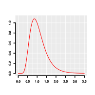
(b)

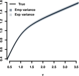
(c)

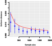
Figure 7: (a) Log-normal density used to sample valuations. (b) True equilibrium bidding function and empirical approximations (in dark grey) and theoretical $\frac{1}{\sqrt{n}}$ confidence bound around true bidding function. (c) Rate of convergence to equilibrium as a function of the sample size, the red line represents the function $0.2/\sqrt{(}n)$.

Proposition 17.

For any $\delta>0$, with probability at least $1-\delta$

$$\max_{i}|\psi(v_{i})-\overline{\boldsymbol{\psi}}_{i}|\\ \leq e^{C}\Big{(}\frac{\log(2/\delta)^{N/2}}{\sqrt{n}}q(n,\delta/2)^{3}+\frac{Cq(n,\delta/2)}{n^{3/2}}\Big{)}$$

Proof.

With the same argument used in Corollary 4 we see that with probability at least $1-\delta$ for $i\leq\frac{1}{n^{3/4}}$ we have $|\psi(v_{i})-\overline{\boldsymbol{\psi}}_{i}|\leq\frac{C}{\sqrt{n}}q(n,\delta)$. On the other hand, since $d\mathbf{M}_{i}=\mathbf{p}_{i}$ the previous Proposition implies that for $i>n^{3/4}$

$$n\big{|}\big{(}d\mathbf{M}^{\prime}(\widehat{\boldsymbol{\psi}}-\overline{\boldsymbol{\psi}})\big{)}_{i}\big{|}\leq C\frac{i^{N-S}}{n^{N-S}}\frac{\log(2/\delta)^{N/2}}{\sqrt{n}}q(n,\delta/2)^{3}.$$

Letting $\epsilon_{i}=|\psi(v_{i})-\overline{\boldsymbol{\psi}}_{i}|$, we see that the previous equation defines the following recursive inequality.

$$nd\mathbf{M}^{\prime}_{ii}\epsilon_{i}\leq C\frac{i^{N-S}}{n^{N-S}}\frac{\log(2/\delta)^{N/2}}{\sqrt{n}}q(n,\delta/2)^{3}\\ -Cn\sum_{j=1}^{i-2}d\mathbf{M}^{\prime}_{ij}\epsilon_{j},$$

where we used the fact that $d\mathbf{M}^{\prime}_{i,i-1}=0$. Since $d\mathbf{M}^{\prime}_{ii}=2\mathbf{M}_{ii}\geq 2\overline{C}\frac{i^{N-S-1}}{n^{N-S-1}}\frac{1}{n}$, after dividing the above inequality by $d\mathbf{M}^{\prime}_{ii}$ we obtain

$$\epsilon_{i}\leq C\frac{\log(2/\delta)^{N/2}}{\sqrt{n}}q(n,\delta/2)^{3}-\frac{C}{n}\sum_{j=1}^{i-2}\epsilon_{j}.$$

Using Lemma 3 again we conclude that

$$\epsilon_{i}\leq e^{C}\Big{(}\frac{\log(2/\delta)^{N/2}}{\sqrt{n}}q(n,\delta/2)^{3}+\frac{Cq(n,\delta/2)}{n^{3/2}}\Big{)}$$

∎

Theorem 3.

If Assumptions 1, 2 and 3 are satisfied, then, for any $\delta>0$, with probability at least $1-\delta$ over the draw of a sample of size $n$, the following bound holds for all $i\in[1,n]$:

$$|\widehat{\beta}(v_{i})-\beta(v_{i})|\leq e^{C}\Big{(}\frac{\log(2/\delta)^{N/2}}{\sqrt{n}}q(n,\delta/2)^{3}+\frac{Cq(n,\delta/2)}{n^{3/2}}\Big{)}.$$

where $q(n,\delta)=\frac{2}{c}\log(nc/2\delta)$ with $c$ defined in Assumption 1, and where $C$ is some universal constant.

Proof.

The proof is a direct consequence of the previous proposition and Proposition 15. ∎

Appendix G EMPIRICAL CONVERGENCE

Here we present an example of convergence by the empirical bidding functions to the true equilibrium bidding function, even when not all technical assumptions are verified. We sampled valuations from a log-normal distribution of parameters $\mu=0$ and $\sigma=0.4$ and calculated the empirical bidding function. Notice that in this case, the support of the distribution is not bounded away from zero (see Figure 7(a). Figure 7(b) shows the true equilibrium bidding function as well as the range of empirical equilibrium functions (in dark grey) obtained after repeating this experiment 10 times. Finally, the region in light gray depicts the predicted theoretical confidence bound in $O(\frac{1}{\sqrt{n}}$. Figure 7(c) shows the rate of uniform convergence to the true equilibrium function as a function of $n$.

References

- Baker (1977) Baker, C. T. (1977). The numerical treatment of integral equations. Clarendon press.
- Börgers et al. (2013) Börgers, T., I. Cox, M. Pesendorfer, and V. Petricek (2013). Equilibrium bids in sponsored search auctions: Theory and evidence. American Economic Journal: Microeconomics 5(4), 163–87.
- Cesa-Bianchi et al. (2013) Cesa-Bianchi, N., C. Gentile, and Y. Mansour (2013). Regret minimization for reserve prices in second-price auctions. In Proceedings of SODA 2013, pp. 1190–1204.
- Edelman et al. (2005) Edelman, B., M. Ostrovsky, and M. Schwarz (2005). Internet advertising and the generalized second price auction: Selling billions of dollars worth of keywords. American Economic Review 97.
- Edelman and Schwarz (2010) Edelman, B. and M. Schwarz (2010). Optimal auction design and equilibrium selection in sponsored search auctions. American Economic Review 100(2), 597–602.
- Gibbons (1992) Gibbons, R. (1992). Game theory for applied economists. Princeton University Press.
- Gomes and Sweeney (2014) Gomes, R. and K. S. Sweeney (2014). Bayes-Nash equilibria of the generalized second-price auction. Games and Economic Behavior 86, 421–437.
- Guerre et al. (2000) Guerre, E., I. Perrigne, and Q. Vuong (2000). Optimal nonparametric estimation of first-price auctions. Econometrica 68(3), 525–574.
- He et al. (2014) He, D., W. Chen, L. Wang, and T. Liu (2014). A game-theoretic machine learning approach for revenue maximization in sponsored search. CoRR abs/1406.0728.
- Kress et al. (1989) Kress, R., V. Maz’ya, and V. Kozlov (1989). Linear integral equations, Volume 82. Springer.
- Lahaie and Pennock (2007) Lahaie, S. and D. M. Pennock (2007). Revenue analysis of a family of ranking rules for keyword auctions. In Proceedings of ACM EC, pp. 50–56.
- Ledoux and Talagrand (2011) Ledoux, M. and M. Talagrand (2011). Probability in Banach spaces. Classics in Mathematics. Berlin: Springer-Verlag. Isoperimetry and processes, Reprint of the 1991 edition.
- Linz (1985) Linz, P. (1985). Analytical and numerical methods for Volterra equations, Volume 7. SIAM.
- Lucier et al. (2012) Lucier, B., R. P. Leme, and É. Tardos (2012). On revenue in the generalized second price auction. In Proceedings of WWW, pp. 361–370.
- Milgrom and Segal (2002) Milgrom, P. and I. Segal (2002). Envelope theorems for aribtrary choice sets. Econometrica 70(2), 583–601.
- Mohri and Medina (2014) Mohri, M. and A. M. Medina (2014). Learning theory and algorithms for revenue optimization in second price auctions with reserve. In Proceedings of ICML, pp. 262–270.
- Myerson (1981) Myerson, R. (1981). Optimal auction design. Mathematics of operations research 6(1), 58–73.
- Ostrovsky and Schwarz (2011) Ostrovsky, M. and M. Schwarz (2011). Reserve prices in internet advertising auctions: a field experiment. In Proceedings of ACM EC, pp. 59–60.
- Pardoe et al. (2005) Pardoe, D., P. Stone, M. Saar-Tsechansky, and K. Tomak (2005). Adaptive auctions: Learning to adjust to bidders. In Proceedings of WITS 2005.
- Qin et al. (2014) Qin, T., W. Chen, and T. Liu (2014). Sponsored search auctions: Recent advances and future directions. ACM TIST 5(4), 60.
- Sun et al. (2014) Sun, Y., Y. Zhou, and X. Deng (2014). Optimal reserve prices in weighted GSP auctions. Electronic Commerce Research and Applications 13(3), 178–187.
- Thompson and Leyton-Brown (2013) Thompson, D. R. M. and K. Leyton-Brown (2013). Revenue optimization in the generalized second-price auction. In Proceedings of ACM EC, pp. 837–852.
- Varian (2007) Varian, H. R. (2007, December). Position auctions. International Journal of Industrial Organization 25(6), 1163–1178.
- Vickrey (1961) Vickrey, W. (1961). Counterspeculation, auctions, and competitive sealed tenders. The Journal of finance 16(1), 8–37.
- Vorobeychik (2009) Vorobeychik, Y. (2009). Simulation-based analysis of keyword auctions. SIGecom Exchanges 8(1).
- Zhu et al. (2009) Zhu, Y., G. Wang, J. Yang, D. Wang, J. Yan, J. Hu, and Z. Chen (2009). Optimizing search engine revenue in sponsored search. In Proceedings of ACM SIGIR, pp. 588–595.