Sequential Empirical Bayes Method for Filtering Dynamic Spatiotemporal Processes

Abstract

We consider online prediction of a latent dynamic spatiotemporal process and estimation of the associated model parameters based on noisy data. The problem is motivated by the analysis of spatial data arriving in real-time and the current parameter estimates and predictions are updated using the new data at a fixed computational cost. Estimation and prediction is performed within an empirical Bayes framework with the aid of Markov chain Monte Carlo samples. Samples for the latent spatial field are generated using a sampling importance resampling algorithm with a skewed-normal proposal and for the temporal parameters using Gibbs sampling with their full conditionals written in terms of sufficient quantities which are updated online. The spatial range parameter is estimated by a novel online implementation of an empirical Bayes method, called herein sequential empirical Bayes method. A simulation study shows that our method gives similar results as an offline Bayesian method. We also find that the skewed-normal proposal improves over the traditional Gaussian proposal. The application of our method is demonstrated for online monitoring of radiation after the Fukushima nuclear accident.

Acknowledgements: This research was conducted during the second author’s visit as a Leverhulme Trust Visiting Fellow at the Department of Mathematical Sciences at the University of Bath whose hospitality is greatly appreciated. Both authors would like to thank the Leverhulme Trust for partial financial support, Grant # VF-2012-006. The second author would like to also thank the Simons Foundation for partial financial support with Grant # 279870, and the Air Force Office of Scientific Research for partial financial support with Grant # FA9550-15-1-0103.

Keywords: Dynamic spatiotemporal process; Empirical Bayes estimation; Fukushima nuclear disaster; Geostatistics; Online inference; State space models.

1 Introduction

Many problems related to ecology, epidemiology, defense, and economics exhibit a simultaneous variability in space and time (CrWi; ShZkbook). Daily levels of precipitation, temperature, or other environmental variables across a region in a year, e.g. the monitoring of pollutants, the estimation of trajectories of biological entities, or the monitoring of mobile threats within a sensor network (Paci201379; RMS; MaNe; RMS2) are a few of a gamut of paradigms which require the careful treatment of spatiotemporal processes in real time.

Our motivation for this study is the monitoring of radiation after the Fukushima nuclear accident. Following the accident, radioactive material was released in the environment which rendered the surrounding areas inhabitable. The authorities established a monitoring program to measure radiation by sampling at specific locations within the infected area. These samples, which are collected daily, can be used to produce a heatmap indicating dangerous zones. This requires spatiotemporal modeling of radiation in real-time to incorporate the new information as soon as it is received. As radiation is measured by the number of nuclear decays emitted each second, a Gaussian model would be inappropriate in this case and a more flexible model is needed.

In cases concerning the study of radiation, disease spreading, weather, and target tracking, where there is no indication when the study will terminate while real-time information must be incorporated to facilitate a rapid-response system, online methods which can assimilate the new data in a fixed computational cost are urgently needed over offline methods. Indeed, the computing costs of offline methods increase commensurately with time and become slower as more and more data are collected. Especially in the modern days of big data, offline methods become inefficient to run for long time periods while online methods are able to take advantage the often-assumed Markov property of the model to simplify computations.

The general setup consists of a latent dynamic process with Markovian evolution while the observation process possesses a conditional independence property. This setup is known as state-space or hidden Markov model. The problem is to compute the filtering distribution, i.e. the distribution of the current value of the latent process given the full observation history up to the present time. A well-known example of an online method is the Kalman filter which gives the exact filtering distribution in the case of linear Gaussian models. A widely-applicable alternative is particle filtering, or sequential Monte-Carlo, which is a sequential importance sampling method that approximates the filtering distribution by a set of weighted samples (DFG). On the other hand, it is well known that particle filtering does not perform well when the dimension of the latent process is large, as is the case of many spatiotemporal applications (CrWi, Section 8.4.6).

In addition to the filtering problem, it is also required to estimate the unknown parameters of the model using the observed data on the fly. In a Bayesian setting, this amounts to computing the posterior distribution of these parameters, however the problem now becomes significantly more difficult as there is no straightforward way of integrating out the latent process in an online fashion. A comprehensive review of online estimation methods can be found in K14. An obvious solution is to augment the latent process with the parameters, and estimate the joint distribution together by standard particle methods. However, this was recognized by Kit that this procedure leads to erroneous estimation. An alternative method, proposed by liuwest, is to impose artificial dynamics on the parameters and estimate them simultaneously with the latent process using particle filters. However, this solution introduces bias in the estimation and requires a significant amount of tuning. The alternative, proposed by Svo; Fea, is to write the full conditionals of the parameters in terms of sufficient statistics which can be updated sequentially. This approach facilitates sampling from the full conditional of the parameters, however it does not avoid the degeneracy problem and is only applicable to those models where sufficient statistics exist, which is not the case for spatial models where the spatial range parameter is unknown.

This manuscript focuses on the methodology for online filtering of a dynamic spatiotemporal process and estimation of the associated static parameters based on data from an exponential family, i.e. the memory and computing time of our method does not grow with time. The inferential procedure derived in this paper is outlined below:

1. For a given spatial range, $\phi$, we develop an online algorithm (Algorithm 1) for sampling from the filtering distribution and the posterior distribution of the other parameters.Our algorithm takes advantage of the skewness of the filtering distribution (see Lemma 1) and produces non-degenerate samples.

2. We develop an online estimate of the Bayes factors corresponding to a finite set of $\phi$ values which we then maximize to estimate $\phi$. The asymptotic validity of our method is established in Theorem 1.

3. Given an estimate of $\phi$, we derive a novel importance resampling algorithm (Algorithm 2) for estimating the latent process and the other parameters in an online fashion.

The rest of the paper is organized as follows. Section 2 discusses the problem formulation and displays preliminary results related to our model, including the derivation of the skew-normal proposal and the proposed algorithm for sampling for fixed $\phi$. Next, Section 3 presents the main contribution of this manuscript and considers the estimation of the spatial correlation via our novel online implementation of the empirical Bayes technique. In Section 4 we illustrate the application of the proposed method for online monitoring of radiation. Section 5 offers a summary and discusses future research directions based on our technique. The proofs to the results presented in the paper are provided in the Appendix. In the Supplementary Materials for this article we present our simulation study for assessing the performance of the proposed method, including a comparison against a typical offline method.

2 Problem formulation and preliminary results

2.1 Model

We adopt a hierarchical, dynamical spatiotemporal model with the observation process $Y$ having conditional independent components from an exponential family distribution given a latent Gaussian spatiotemporal field $X$.

Let $\mathbb{S}$ denote the continuous spatial domain of interest and let $\mathbb{T}=\{0,1,2,\ldots\}$ be the temporal domain. The process model consists of a spatiotemporal Gaussian process $X$ on $\mathbb{S}\times\mathbb{T}$ having an autoregressive structure, that is, for every finite collection of spatial locations in $\mathbb{S}$, say of size $n$, the value of $X$ at the $n$ locations at time $t$, ${\mathbf{x}}_{t}$, is described by a perturbation of its values at time $t-1$, ${\mathbf{x}}_{t-1}$, as follows

$${\mathbf{x}}_{0}=G_{0}\beta+\sigma\epsilon_{0},\quad{\mathbf{x}}_{t}=G_{t}\beta+\alpha({\mathbf{x}}_{t-1}-G_{t-1}\beta)+\sigma\epsilon_{t},\ t=1,2,\ldots$$ (1)

where the driving noise is a normally distributed isotropic spatial process, $\epsilon_{t}\sim N_{n}(0,R(\phi))$, $G_{t}$ defines the $n\times m$ matrix of covariates for each time $t$ associated with an $m\times 1$ parameter vector $\beta$, $\sigma$ is the diffusion coefficient and $\phi$ denotes the range parameter with spatial correlation matrix $R=R(\phi)$. Our model assumes linear transition in time. In general, $\alpha$ is an $n\times n$ matrix of redistribution weights, however, as CrWi argue in Section 7.2, this can be challenging to estimate at early times. A simpler model that allows stationarity is to let $\alpha$ be a scalar, where $|\alpha|<1$. This implies homogeneous transition between the components of the state process. The theory developed in this paper applies to either matrix or scalar $\alpha$ but the issues we wish to address can be illustrated more clearly when $\alpha$ is a scalar so we will focus on this case for the remainder of this paper.

The observation process $Y$ is defined on $\mathbb{S}\times\mathbb{T}$ and is assumed to have conditionally independent components given the latent spatiotemporal process $X$ with distribution from an exponential family. In other words, let $y_{i,t}$ denote the value of the observation process at location $i$ and time $t$, and let $x_{i,t}$ denote the value of the corresponding spatiotemporal process. Then

$$p(y_{i,t}|x_{i,t})\propto\exp\{y_{i,t}g(x_{i,t})-\tau_{i,t}b(x_{i,t})\},$$ (2)

where under the usual regularity assumptions for exponential families the mean of the distribution in (2) is $h({x}_{i,t})$ with $h(\cdot)$ being the inverse link function, $g(\cdot)$ and $b(\cdot)$ are known functions and $\tau_{i,t}$ is a known scalar associated with the underlying distribution of the data. Further, given $x_{i,t}$, $y_{i,t}$ is independent of every other component of $Y$. The main advantage in using the general state space representation of a dynamic spatiotemporal process is that we do not need to rely on the normality assumption for the observation process and thus nonlinear and/or non-Gaussian models could be taken into account.

For the parameters $(\beta,\alpha)$ we assume a normal prior, although the methodology described here is valid for truncated normal or improper uniform priors as well, and the variance coefficient $\sigma^{2}$ is assumed to be distributed according to an inverse-gamma conjugate prior, i.e.

$$\begin{gathered}\beta|\sigma^{2}\sim N_{m}(Q_{0}^{-1}b_{0},\sigma^{2}Q_{0}^{-1}),\\ \alpha|\sigma^{2}\sim N(s_{0}^{-1}a_{0},\sigma^{2}s_{0}^{-1}),\\ \sigma^{2}\sim IG\left(\frac{c_{0}}{2},\frac{r_{0}}{2}\right),\end{gathered}$$ (3)

for suitable hyperparameters $b_{0}$, $Q_{0}$, $a_{0}$, $s_{0}$, $c_{0}$, and $r_{0}$. To make the priors reasonably uninformative it is common to set $Q_{0}=q_{0}I$, i.e. a diagonal with all diagonal elements equal to $q_{0}$, and assign small values to $q_{0}$, $s_{0}$, $c_{0}$ and $r_{0}$. If $\alpha$ is a matrix, as was discussed earlier, then matrix-normal prior is used instead.

2.2 Bayesian inference

We assume that observations from $n$ fixed spatial locations are available at times $1,2,\ldots$, but we do not assume that all $n$ locations are observed every time. We denote by ${\mathbf{y}}_{1:t}=({\mathbf{y}}_{1},{\mathbf{y}}_{2},\ldots,{\mathbf{y}}_{t})$ the observations up to time $t$ where each ${\mathbf{y}}_{s}$ is an $n$-dimensional vector, possibly containing missing values. We denote by ${\mathbf{x}}_{0:t}=({\mathbf{x}}_{0},{\mathbf{x}}_{1},\ldots,{\mathbf{x}}_{t})$ the value of the spatiotemporal process at the same $n$ locations up to time $t$, and $\theta=(\alpha,\beta,\sigma^{2})$ denotes the temporal parameters. The problem is to estimate the parameters $\theta$ and $\phi$, as well as the latent process at time $t$, ${\mathbf{x}}_{t}$, from the available data ${\mathbf{y}}_{1:t}$. The problem of estimating the spatiotemporal process at locations different from the sampled locations becomes trivial after $\theta$, $\phi$, and ${\mathbf{x}}_{0:t}$ are estimated.

For given $\phi$, we sample from the posterior distribution $p({\mathbf{x}}_{0:t},\theta|{\mathbf{y}}_{1:t},\phi)$ by combining the particle filter resampling method with a skewed proposal and the sufficient statistics method of Svo and Fea. The setup of Section 2.1 allows sampling from the full conditional distribution of the parameters $\theta$ via Gibbs sampling.

More precisely, the full conditional distribution of the parameter $\beta$ is

$$p(\beta|{\mathbf{x}}_{0:t},{\mathbf{y}}_{1:t},\alpha,\sigma^{2},\phi)\propto p(\beta)\prod_{s=1}^{t}p({\mathbf{x}}_{s}|{\mathbf{x}}_{s-1},\alpha,\beta,\sigma^{2},\phi),$$

which is easily shown to be normal $\beta|({\mathbf{x}}_{0:t},{\mathbf{y}}_{1:t},\alpha,\sigma^{2},\phi)\sim N_{m}(Q_{t}^{-1}b_{t},\sigma^{2}Q_{t}^{-1})$, where

$$Q_{t} =Q_{0}+G_{0}^{\prime}R^{-1}G_{0}+\sum_{s=1}^{t}(G_{s}-\alpha G_{s-1})^{\prime}R^{-1}(G_{s}-\alpha G_{s-1}),$$ (4)

$$b_{t} =b_{0}+G_{0}^{\prime}R^{-1}{\mathbf{x}}_{0}+\sum_{s=1}^{t}(G_{s}-\alpha G_{s-1})^{\prime}R^{-1}({\mathbf{x}}_{s}-\alpha{\mathbf{x}}_{s-1}),$$

and similarly for $\alpha$ and $\sigma^{2}$. Note that the full conditional distributions of $\theta=(\alpha,\beta,\sigma^{2})$ depend on some sufficient quantities, $u_{t}=u_{t}({\mathbf{x}}_{0:t},\phi)$, which are updated recursively. (We use the term “sufficient quantities” instead of “sufficient statistics” because they depend on the unknown parameter $\phi$.) For example, to update $\beta$, from (4), we need to keep a record of the sums $\sum G_{s}^{\prime}R^{-1}G_{s}$, $\sum G_{s}^{\prime}R^{-1}G_{s-1}$, $\sum G_{s}^{\prime}R^{-1}{\mathbf{x}}_{s}$, $\sum G_{s}^{\prime}R^{-1}{\mathbf{x}}_{s-1}$, and $\sum G_{s-1}^{\prime}R^{-1}{\mathbf{x}}_{s}$ where the summation is over $s=1,\ldots,t$. Having stored the sufficient quantities $u_{t-1}({\mathbf{x}}_{0:t-1},\phi)$ at time $t-1$, we update them by adding the corresponding terms at time $t$, i.e. $u_{t}({\mathbf{x}}_{0:t},\phi)=\mathcal{U}(u_{t-1}({\mathbf{x}}_{0:t-1},\phi),{\mathbf{x}}_{t},\phi)$.

To sample $({\mathbf{x}}_{t},\theta)$ we take marginal samples from $p({\mathbf{x}}_{0:t},\theta|{\mathbf{y}}_{1:t},\phi)$. The key element in the process for doing so, given a sample from $p({\mathbf{x}}_{0:t-1}|{\mathbf{y}}_{1:t-1},\phi)$, is

$$p({\mathbf{x}}_{0:t},\theta|{\mathbf{y}}_{1:t},\phi)\propto p({\mathbf{y}}_{t}|{\mathbf{x}}_{t})p(\theta|{\mathbf{x}}_{0:t-1},\phi)p({\mathbf{x}}_{t}|{\mathbf{x}}_{t-1},\theta,\phi)p({\mathbf{x}}_{0:t-1}|{\mathbf{y}}_{1:t-1},\phi),$$

which suggests a separate, two-step, update for $\theta$ and ${\mathbf{x}}_{t}$. In the first step we sample $\theta$ from $p(\theta|{\mathbf{x}}_{0:t-1},\phi)=p(\theta|u_{t-1}({\mathbf{x}}_{0:t-1},\phi))$. Because this distribution is not available in closed form but the full conditional distributions for each component of $\theta$ given the other components are, sampling is done by running a few Gibbs iterations for each component of $\theta$. The final $\theta$ obtained at the end of the sequence of Gibbs iterations, together with ${\mathbf{x}}_{t-1}$ and ${\mathbf{y}}_{t}$ are used to sample ${\mathbf{x}}_{t}$. To that end, let $q({\mathbf{x}}_{t}|{\mathbf{x}}_{t-1},{\mathbf{y}}_{t},\theta,\phi)$ be a proposal distribution which generates $N$ particles $\tilde{\mathbf{x}}^{(1)},\ldots,\tilde{\mathbf{x}}^{(N)}$. Each particle carries a weight proportional to

$$w^{(i)}=\frac{p({\mathbf{y}}_{t}|\tilde{\mathbf{x}}_{t}^{(i)})p(\tilde{\mathbf{x}}_{t}^{(i)}|{\mathbf{x}}_{t-1},\theta,\phi)}{q(\tilde{\mathbf{x}}_{t}^{(i)}|{\mathbf{x}}_{t-1},{\mathbf{y}}_{1:t},\theta,\phi)}.$$ (5)

The sample ${\mathbf{x}}_{t}$ is chosen from among the $\tilde{\mathbf{x}}^{(1)},\ldots,\tilde{\mathbf{x}}^{(N)}$ with weights proportional to $w^{(1)},\ldots,w^{(N)}$. Algorithm 1 outlines the steps from this procedure.

Algorithm 1 One step sampling for fixed $\phi$ at time $t$.

0:   ${\mathbf{y}}_{t}$; Sample ${\mathbf{x}}_{t-1}\sim p({\mathbf{x}}_{t-1}|{\mathbf{y}}_{1:t-1},\phi)$;Sufficient quantities $u_{t-1}=u_{t-1}({\mathbf{x}}_{0:t-1},\phi)$.

0:  

1:  Sample $\theta$ from $p(\theta|u_{t-1})$ by running a few Gibbs iterations.

2:  Compute the proposal $q({\mathbf{x}}_{t}|{\mathbf{x}}_{t-1},{\mathbf{y}}_{t},\theta,\phi)$.

3:  Sample $\tilde{\mathbf{x}}_{t}^{(1)},\ldots,\tilde{\mathbf{x}}_{t}^{(N)}\sim q({\mathbf{x}}_{t}|{\mathbf{x}}_{t-1},{\mathbf{y}}_{t},\theta,\phi)$.

4:  Compute the weight $w^{(i)}$ according to (5) for $i=1,\ldots,N$.

5:  Sample index $j$ from $\{1,\ldots,N\}$ with weights proportional to $w^{(1)},\ldots,w^{(N)}$.

6:  Set ${\mathbf{x}}_{t}=\tilde{\mathbf{x}}_{t}^{(j)}$

7:  Update the sufficient quantities $u_{t}=\mathcal{U}(u_{t-1},{\mathbf{x}}_{t},\phi)$.

7:   ${\mathbf{x}}_{t}$, $u_{t}$, $\theta$.

On the other hand, implementing the same approach for the estimation of the range parameter $\phi$ is far from trivial and it cannot be updated using sufficient quantities as before, making it impractical for online applications. Furthermore, each update of $\phi$ requires the inversion of a large matrix which could be computationally expensive when the dimension of the random field, $n$, is large. Therefore a technique other than Gibbs sampling (or in general an MCMC framework) is required. We circumvent this problem by using a novel particle filter with an online implementation of an empirical Bayes method. This technique is treated next in Section 3.

2.3 A skewed-normal proposal density

A measure of the quality of the proposal distribution is the effective sample size (ESS), defined as

$$\mathrm{ESS}=\frac{(\sum_{i}w^{i}_{t})^{2}}{\sum_{i}(w^{i}_{t})^{2}}.$$

It can take values between 1 and $N$ and is used for assessing the loss of variance in the importance weights (RobertCasella, Section 4.4). A value close to $N$ would mean that the samples are nearly equally weighted and there is diversity among the samples so no samples are lost. A value close to 1 would indicate that all but one sample will have weight close to 0 and lead to the well-known problem of sample degeneracy.

Importance sampling methods allow flexibility in the choice of the proposal distribution $q$ but as DGA point out the optimal proposal distribution in the sense that it minimizes the variance of the importance weights is

$$q({\mathbf{x}}_{t}|{\mathbf{x}}_{t-1},{\mathbf{y}}_{1:t},\theta,\phi)=p({\mathbf{x}}_{t}|{\mathbf{x}}_{t-1},{\mathbf{y}}_{t},\theta,\phi).$$ (6)

Although not helpful by itself, equation (6) is still useful since it can serve as a basis for deriving suboptimal proposal distributions. One way of doing this approximates (6) by a multivariate Gaussian distribution as was done by DGA in the univariate case. When the state process is multivariate it is imperative to use a good proposal density as this increases the effective sample size. In view of this, we introduce next a novel importance density. First, Lemma 1 shows that the optimal proposal distribution is skewed when the observation process has a skewed distribution. This suggests using a proposal distribution which is skewed and motivates our use of the skewed-normal distribution for this purpose.

Lemma 1.

Consider the stochastic dynamics in equation (1) and the observation process given in equation (2) which corresponds to data from a general exponential family. Then the optimal proposal distribution given in equation (6) is skewed when the likelihood of $y_{i,t}|x_{i,t}$ is skewed.

Proof..

See Appendix. ∎

Consider first a Gaussian approximation to (6). Note that the optimal proposal is $p({\mathbf{x}}_{t}|{\mathbf{x}}_{t-1},{\mathbf{y}}_{t},\theta,\phi)\propto p({\mathbf{y}}_{t}|{\mathbf{x}}_{t})p({\mathbf{x}}_{t}|{\mathbf{x}}_{t-1},\theta,\phi)$ and let

$$f({\mathbf{x}}_{t})=-\log\{p({\mathbf{y}}_{t}|{\mathbf{x}}_{t})p({\mathbf{x}}_{t}|{\mathbf{x}}_{t-1},\theta,\phi)\}.$$ (7)

Next define

$$\hat{\mathbf{x}}_{t}=\operatorname*{argmin}_{{\mathbf{x}}_{t}}f({\mathbf{x}}_{t}),\qquad\hat{H}_{t}=\nabla\nabla^{\prime}f(\hat{\mathbf{x}}_{t}).$$

The Gaussian proposal is constructed by setting the mean equal to $\hat{{\mathbf{x}}}_{t}$ and the variance to $\hat{H}_{t}^{-1}$.

To capture the skewness of the distribution we use a skewed-normal copula correction to the Gaussian proposal. The probability density function (pdf) of the univariate skewed-normal distribution is (AC:SN)

$$\frac{2}{\omega}\,\psi\!\left(\frac{z-\xi}{\omega}\right)\Psi\!\left(a\frac{z-\xi}{\omega}\right)$$

where $\psi(\cdot)$ and $\Psi(\cdot)$ denote the pdf and cumulative distribution function (cdf) of the standard normal distribution respectively. The parameters $\xi$, $\omega>0$, and $a$ correspond to the location, scale, and skewness parameter respectively.

To derive the skewed-normal corrections we expand the marginals of (7) to third order terms and match the first three moments to the skewed-normal distribution. For details see Appendix B of rue2009approximate. Let $\tilde{\mathbf{x}}_{t}$ be a sample from the Gaussian approximation to (6). The idea is to transform $\tilde{\mathbf{x}}_{t}$ marginally using the skewed-normal correction. ferkingstad2015 propose two copula corrections which we also use here: a mean-only skewness correction where the proposal distribution remains Gaussian but the mean is corrected using the skewed-normal approximations to the marginals; and a mean-plus-skewness correction where the particles are sampled from the Gaussian approximation and then are marginally transformed using the skewed-normal approximation. In our simulation study (see Supplementary Materials, Section 1) we find that the two skewed-normal proposals have similar ESS but the Gaussian proposal has significantly lower ESS. We therefore recommend the mean-only corrected proposal because it is simpler than the mean-plus-skewness correction, while it also has better ESS than the Gaussian proposal.

3 A methodology for online estimation and prediction

In this section we present an empirical Bayes approach for the estimation of the range parameter $\phi$. Unlike the parameter $\theta=(\alpha,\beta,\sigma^{2})$, it is not possible to include $\phi$ as an extra step in the Gibbs algorithm without sacrificing the online feature of the method since the sufficient quantities for the update of $\theta$ depend on $\phi$ and consequently they must be recomputed from time one at every update of $\phi$. Instead we adopt a novel empirical Bayes method in order to estimate $\phi$ in a way that is similar in spirit to Doss. Another argument in favor of the empirical Bayes approach instead of a full Bayesian approach is that it is unclear how a suitable prior for $\phi$ should be chosen. BOS discuss some objective priors in the case of Gaussian responses. However for non-Gaussian data these priors, and indeed any improper prior, result in an improper posterior for $\phi$ (CMW). When it comes to online inference, it is unclear how a fully Bayesian approach would be implemented. If a Monte-Carlo algorithm is used, the sufficient quantities will be computed for those $\phi$ values in the Monte-Carlo sample only. This restricts the $\phi$ values at subsequent times to only those which were sampled at all previous time points, something that is undesirable. The goodness-of-fit of the empirical Bayes method for estimating the range parameter has been demonstrated in the case of the spatial-only model by roy16. Extending it to an online version requires careful treatment of the sufficient quantities needed to compute the Bayes factors. Theorem 1 presents the main result of this section. The approach discussed below may be also viewed as equivalent to the maximum likelihood estimation for $\phi$ after integrating out the parameter $\theta$.

We consider first the marginal density $p({\mathbf{y}}_{1:t}|\phi)$ and define the estimator for $\phi$ at time $t$ given data ${\mathbf{y}}_{1:t}$ by

$$\hat{\phi}_{t}=\operatorname*{argmax}_{\phi}p({\mathbf{y}}_{1:t}|\phi),$$ (8)

where

$$p({\mathbf{y}}_{1:t}|\phi)=\int p({\mathbf{y}}_{1:t},{\mathbf{x}}_{0:t},\theta|\phi)d({\mathbf{x}}_{0:t},\theta).$$ (9)

In general, the integral in (9) has no closed form and thus a numerical approximation must be employed. Define the sequential Bayes factor between $\phi$ and $\tilde{\phi}$ with respect to the data ${\mathbf{y}}_{1:t}$ by

$$B_{1:t}(\phi;\tilde{\phi})=\frac{p({\mathbf{y}}_{1:t}|\phi)}{p({\mathbf{y}}_{1:t}|\tilde{\phi})}.$$

Note the dependence of the Bayes factor on the whole data sequence ${\mathbf{y}}_{1:t}$. Then, for a fixed parameter $\tilde{\phi}$, (8) is equivalent to

$$\hat{\phi}_{t}=\operatorname*{argmax}_{\phi}B_{1:t}(\phi;\tilde{\phi}).$$

Furthermore, the sequential Bayes factor, $B_{1:t}(\phi;\tilde{\phi})$ in a filtering framework is computed as follows:

$$B_{1:t}(\phi;\tilde{\phi}) =\int\frac{p({\mathbf{y}}_{1:t},{\mathbf{x}}_{0:t},\theta|\phi)}{p({\mathbf{y}}_{1:t},{\mathbf{x}}_{0:t},\theta|\tilde{\phi})}p({\mathbf{x}}_{0:t},\theta|{\mathbf{y}}_{1:t},\tilde{\phi})d({\mathbf{x}}_{0:t},\theta)$$ (10)

$$=\int\frac{p({\mathbf{y}}_{1:t}|{\mathbf{x}}_{0:t})p({\mathbf{x}}_{0:t}|\theta,\phi)p(\theta)}{p({\mathbf{y}}_{1:t}|{\mathbf{x}}_{0:t})p({\mathbf{x}}_{0:t}|\theta,\tilde{\phi})p(\theta)}p({\mathbf{x}}_{0:t},\theta|{\mathbf{y}}_{1:t},\tilde{\phi})d({\mathbf{x}}_{0:t},\theta)$$

$$=\int\frac{p({\mathbf{x}}_{0:t}|\theta,\phi)}{p({\mathbf{x}}_{0:t}|\theta,\tilde{\phi})}p({\mathbf{x}}_{0:t},\theta|{\mathbf{y}}_{1:t},\tilde{\phi})d({\mathbf{x}}_{0:t},\theta).$$

A naive approach for estimating $\phi$ relying on equation (10) would be to obtain a large sample for $({\mathbf{x}}_{0:t},\theta)$ from $p({\mathbf{x}}_{0:t},\theta|{\mathbf{y}}_{1:t},\tilde{\phi})$ using Algorithm 1, and to approximate (10) by Monte-Carlo integration; call the result $\hat{B}_{1:t}(\phi;\tilde{\phi})$. Then an estimate would be obtained by maximizing $\hat{B}_{1:t}(\phi;\tilde{\phi})$ over $\phi$.

Remark 1.

There are several issues concerning the above naive approach that need to be addressed:

1. Unless $\hat{\phi}_{t}$ and $\tilde{\phi}$ are close to one another, the Monte-Carlo approximation will have a large error and in this case the estimate may not be accurate no matter how large the Monte-Carlo sample is.

2. In order to compute $p({\mathbf{x}}_{0:t}|\theta,{\phi})$ for any $\phi$ at time-point $t$, we need $p({\mathbf{x}}_{0:t-1}|\theta,{\phi})$ for the same $\phi$ at time $t-1$ something that we could not anticipate prior to time $t$.

3. After obtaining $\hat{\phi}_{t}$ we need to run Algorithm 1 once more in order to update ${\mathbf{x}}_{t}$ and $\theta$ conditional on $\hat{\phi}_{t}$. However the algorithm requires samples from ${\mathbf{x}}_{0:t-1}|{\mathbf{y}}_{1:t-1},\hat{\phi}_{t}$ which is unknown at time $t-1$.

Bypassing the issues raised in Remark 1, our strategy for resolving issue 1 is to replace the importance density in (10) by a mixture over a set of $\phi$ values instead of a single fixed $\tilde{\phi}$. This is demonstrated in our simulation study (see Supplementary Materials, Section 2) where we show that the naive approach can give biased estimates for a badly chosen $\tilde{\phi}$. For 2 we only evaluate the Bayes factors over a dense grid $\Phi$ which covers reasonable values of $\phi$ and keeps a record of the sufficient quantities needed to evaluate $p({\mathbf{x}}_{0:t}|\theta,{\phi})$ at the next time. To resolve 3 we resample the available samples from the mixture with appropriate weights. In the remainder of this section we expand on these ideas. Algorithm 2 puts them together.

Consider a set $\Phi_{K}=\{\phi_{1},\ldots,\phi_{K}\}$ such that $\tilde{\phi}\in\Phi_{K}$, is sufficiently spread-out over a range of interesting values of $\phi$. The meaning of “interesting values of $\phi$” is well defined in our context: the range parameter is a scaling factor of the spatial distances within the domain of interest which define a possible range for $\phi$. Suppose $({\mathbf{x}}_{0:t}^{(l,k)},\theta^{(l,k)})$, $k=1,\ldots,K$, $l=1,\ldots,L_{k}$ are samples from $p({\mathbf{x}}_{0:t},\theta|{\mathbf{y}}_{1:t},\phi_{k})$. The augmented sample can be seen as drawn from the mixture distribution

$$p_{\text{mix}}({\mathbf{x}}_{0:t},\theta|{\mathbf{y}}_{1:t},\Phi_{K},\Lambda_{K})=\sum_{k=1}^{K}\lambda_{k}p({\mathbf{x}}_{0:t},\theta|{\mathbf{y}}_{1:t},\phi_{k}),$$ (11)

where $\lambda_{k}=L_{k}/(\sum L_{k^{\prime}})$ and $\Lambda_{K}=\{\lambda_{1},\ldots,\lambda_{K}\}$. Let $b_{t}^{k}=B_{1:t}(\phi_{k};\tilde{\phi})$. Then $b_{t}^{k}$ can be estimated by maximizing the so-called reverse logistic log-likelihood (Gey)

$$\ell(\mathbf{b}_{t})=\sum_{k=1}^{K}\sum_{l=1}^{L_{k}}\log\frac{\lambda_{k}p({\mathbf{x}}_{0:t}^{(k,l)},\theta^{(k,l)}|{\mathbf{y}}_{1:t},\phi_{k})}{p_{\text{{mix}}}({\mathbf{x}}_{0:t}^{(k,l)},\theta^{(k,l)}|{\mathbf{y}}_{1:t},\Phi_{K},\Lambda_{K})}.$$

Furthermore, let $\hat{b}_{t}^{k}$ denote the estimate for $b_{t}^{k}$. Then, the following sum

$$\hat{B}_{1:t}(\phi;\tilde{\phi})=\sum_{k=1}^{K}\sum_{l=1}^{L_{k}}\frac{p({\mathbf{x}}_{0:t}^{(k,l)}|\theta^{(k,l)},\phi)}{\sum_{k^{\prime}}{L_{k^{\prime}}}/{\hat{b}^{k^{\prime}}_{t}}p({\mathbf{x}}_{0:t}^{(k,l)}|\theta^{(k,l)},\phi_{k^{\prime}})},$$ (12)

estimates $B_{1:t}(\phi;\tilde{\phi})$. The key Theorem 1 summarizes this property.

Theorem 1.

Consider a coarse grid $\Phi_{K}=\{\phi_{1},\phi_{2},\ldots,\phi_{K}\}$, where the grid points, $\phi_{k}$, $k=1,\ldots,K$, are spaced across the parameter space for $\phi$. Suppose that for $k=1,\ldots,K$, we draw samples $({\mathbf{x}}^{(k,l)}_{1:t},\theta^{(k,l)})$, $l=1,\ldots,L_{k}$ from the distribution $p({\mathbf{x}}_{0:t},\theta|\phi_{k},{\mathbf{y}}_{1:t})$ for $\phi_{k}\in\Phi_{K}$. Then, for an arbitrarily fixed pair $(\phi,\tilde{\phi})$, the estimate,

$$\hat{B}_{1:t}(\phi;\tilde{\phi})\stackrel{{\scriptstyle\mbox{a.s.}}}{{\longrightarrow}}B_{1:t}(\phi;\tilde{\phi}),\;\;L_{k}\to\infty,$$ (13)

where $\hat{B}_{1:t}(\phi;\tilde{\phi})$ is given by equation (12).

Proof..

See Appendix. ∎

The likelihood in the numerator and denominator of (12) must be computed for the whole history of samples ${\mathbf{x}}_{0:t}^{(k,l)}$ for the new $\theta^{(k,l)}$ and for different values of $\phi$. This is not as straightforward as a product of the prior $p({\mathbf{x}}_{0:t-1}|\theta,\phi)$ times the transition $p({\mathbf{x}}_{t}|{\mathbf{x}}_{t-1},\theta,\phi)$ since in online implementations we cannot anticipate the value of $\theta$ and $\phi$ at time $t-1$. If $\phi$ is held fixed, then $p({\mathbf{x}}_{0:t}|\theta,\phi)$ can be written in terms of sufficient quantities as before which do not depend on $\theta$ but do depend on $\phi$.

To this end, let $z_{t-1}^{(\phi,k,l)}$ denote the aforementioned sufficient quantities at time $t-1$ for the $(k,l)$th sample. These are updated at time $t$ by

$$z_{t}^{(\phi,k,l)}=\mathcal{Z}\left(z_{t-1}^{(\phi,k,l)},{\mathbf{x}}_{t}^{(k,l)},\phi\right),$$

and the joint likelihood is expressed as a function of $z_{t}^{(\phi,k,l)}$ and $\theta^{(k,l)}$, i.e.

$$p({\mathbf{x}}_{0:t}^{(k,l)}|\theta^{(k,l)},\phi)=\mathcal{P}\left(z_{t}^{(\phi,k,l)},\theta^{(k,l)}\right).$$

In practice, we do not consider the entire parameter space for $\phi$ but a fine discretization of it. More precisely, we augment the coarse grid, $\Phi_{K},$ with the finer grid, say $\Phi$, i.e. $\Phi_{K}\subset\Phi$, and compute the sufficient quantities $z_{t}^{(\phi,k,l)}$, and consequently $\hat{B}_{1:t}(\phi;\tilde{\phi})$, only for those $\phi\in\Phi$. Then, we estimate $\phi$ by

$$\hat{\phi}_{t}=\operatorname*{argmax}_{\phi\in\Phi}\hat{B}(\phi;\tilde{\phi}).$$

The drawback is the loss of precision in estimation but the benefit is that the required computing memory remains fixed. From experience, we find that a small bias in the value of $\phi$ does not affect prediction or the estimation of the other parameters. In particular in the simulation study presented in Section 2 of the Supplementary Materials we find that the parameters $\alpha$ and $\beta$ are immune to the possible bias in $\hat{\phi}_{t}$.

The empirical Bayes approach proceeds with the update of the estimate for $({\mathbf{x}}_{t},\theta)$ using the estimate $\hat{\phi}_{t}$. These estimates are obtained as a weighted sum of the existing samples $({\mathbf{x}}_{0:t}^{(k,l)},\theta^{(k,l)})$, $k=1,\ldots,K$, $l=1,\ldots,L_{k}$. The distribution of the existing samples is the mixture distribution (11). These samples can be scaled with reference to the distribution conditioned on $\phi=\hat{\phi}_{t}$ using the following importance weights

$$v_{t}^{(k,l)} =\frac{p({\mathbf{x}}_{0:t}^{(k,l)},\theta^{(k,l)}|{\mathbf{y}}_{1:t},\hat{\phi}_{t})}{p_{\text{mix}}({\mathbf{x}}_{0:t}^{(k,l)},\theta^{(k,l)}|{\mathbf{y}}_{1:t},\Phi_{K},\Lambda_{K})}=\frac{p({\mathbf{x}}_{0:t}^{(k,l)},\theta^{(k,l)}|{\mathbf{y}}_{1:t},\hat{\phi}_{t})}{\sum_{k^{\prime}}\lambda_{k^{\prime}}p({\mathbf{x}}_{0:t}^{(k,l)},\theta^{(k,l)}|{\mathbf{y}}_{1:t},\phi_{k^{\prime}})}$$

$$=\frac{p({\mathbf{y}}_{1:t}|{\mathbf{x}}_{0:t}^{(k,l)})p({\mathbf{x}}_{0:t}^{(k,l)}|\theta^{(k,l)},\hat{\phi}_{t})p(\theta^{(k,l)})/p({\mathbf{y}}_{1:t}|\hat{\phi}_{t})}{\sum_{k^{\prime}}\lambda_{k^{\prime}}p({\mathbf{y}}_{1:t}|{\mathbf{x}}_{0:t}^{(k,l)})p({\mathbf{x}}_{0:t}^{(k,l)}|\theta^{(k,l)},\phi_{k^{\prime}})p(\theta^{(k,l)})/p({\mathbf{y}}_{1:t}|\phi_{k^{\prime}})}$$

$$=\frac{p({\mathbf{x}}_{0:t}^{(k,l)}|\theta^{(k,l)},\hat{\phi}_{t})/B_{1:t}(\hat{\phi}_{t};\tilde{\phi})}{\sum_{k^{\prime}}\lambda_{k^{\prime}}p({\mathbf{x}}_{0:t}^{(k,l)}|\theta^{(k,l)},\phi_{k^{\prime}})/B_{1:t}(\phi_{k^{\prime}};\tilde{\phi})}.$$ (14)

In practice $B_{1:t}(\hat{\phi}_{t};\tilde{\phi})$ and $B_{1:t}(\phi_{k^{\prime}};\tilde{\phi})$ in equation (3) are replaced by their estimates which are already available. Then, we obtain the estimates for the latent state process and the remaining parameters by

$$\hat{\mathbf{x}}_{t}=\sum_{k=1}^{K}\sum_{l=1}^{L_{k}}\bar{v}_{t}^{(k,l)}{\mathbf{x}}_{t}^{(k,l)},\quad\hat{\theta}_{t}=\sum_{k=1}^{K}\sum_{l=1}^{L_{k}}\bar{v}_{t}^{(k,l)}\theta^{(k,l)},$$

where $\bar{v}_{t}^{(k,l)}$ is the normalized version of (3). This is the final step at time $t$. The main algorithm of this paper which shows how to combine Algorithm 1 with the online empirical Bayes for the estimation of $\phi$ is displayed in Algorithm 2.

Algorithm 2 Main estimation and prediction algorithm at time $t$.

0:   ${\mathbf{y}}_{t}$; Samples ${\mathbf{x}}_{t-1}^{(k,1:L_{k})}\sim p({\mathbf{x}}_{t-1}|{\mathbf{y}}_{1:t-1},\phi_{k})$, $k=1,\ldots,K$; Sufficient quantities $u_{t-1}^{(k,1:L_{k})}$, $k=1,\ldots,K$;Sufficient quantities $z_{t-1}^{(\phi,k,1:L_{k})}$, $\phi\in\Phi$, $k=1,\ldots,K$.

0:  

1:  for $k\in\{1,\ldots,K\}$ do concurrently

2:     for $l=1,\ldots,L_{k}$ do concurrently

3:        Sample $l^{\prime}$ uniformly in $\{1,\ldots,L_{k}\}$.

4:        Call Algorithm 1 with input ${\mathbf{y}}_{t}$, ${\mathbf{x}}_{t-1}^{(k,l^{\prime})}$, $u_{t-1}^{(k,l^{\prime})}$, and output $\theta^{(k,l)}$, ${\mathbf{x}}_{t}^{(k,l)}$, $u_{t}^{(k,l)}$.

5:        for $\phi\in\Phi$ do concurrently

6:           Update the sufficient quantities $z_{t}^{(\phi,k,l)}=\mathcal{Z}\left(z_{t-1}^{(\phi,k,l)},{\mathbf{x}}_{t}^{(k,l)},\phi\right)$.

7:           Compute $p({\mathbf{x}}_{0:t}^{(k,l)}|\theta^{(k,l)},\phi)=\mathcal{P}\left(z_{t}^{(\phi,k,l)},\theta^{(k,l)}\right)$.

8:        end for $\phi$

9:     end for $l$

10:  end for $k$

11:  Call the reverse logistic regression algorithm with input $\{p({\mathbf{x}}_{0:t}^{(k,1:L_{k})}|\theta^{(k,1:L_{k})},\phi):\phi\in\Phi,k=1,\ldots,K\}$ and output $\hat{\mathbf{b}}_{t}$.

12:  Compute $\hat{B}_{1:t}(\phi;\tilde{\phi})$, $\phi\in\Phi$ using (12).

13:  Set $\hat{\phi}_{t}=\operatorname*{argmax}_{\phi\in\Phi}\hat{B}_{1:t}(\phi;\tilde{\phi})$.

14:  Compute importance weights $v_{t}^{(k,l)}$ according to equation (3) and normalize them to get $\bar{v}_{t}^{(k,l)}$.

15:  Set $\hat{\mathbf{x}}_{t}=\sum_{k=1}^{K}\sum_{l=1}^{L_{k}}\bar{v}_{t}^{(k,l)}{\mathbf{x}}_{t}^{(k,l)}$, $\hat{\theta}_{t}=\sum_{k=1}^{K}\sum_{l=1}^{L_{k}}\bar{v}_{t}^{(k,l)}\theta^{(k,l)}$.

15:   $\hat{\mathbf{x}}_{t}$, $\hat{\theta}_{t}$, $\hat{\phi}_{t}$, ${\mathbf{x}}_{t}^{(k,1:L_{k})}$, $\theta^{(k,1:L_{k})}$, $u_{t}^{(k,1:L_{k})}$, $k=1,\ldots,K$,$z_{t}^{(\phi,k,1:L_{k})}$, $\phi\in\Phi$, $k=1,\ldots,K$.

We evaluated the performance of our method in a simulation study which we include in the Supplementary Materials with this article. Our study shows that the obtained parameter estimates are unbiased and consistent. As more data are assimilated, the credible intervals obtained from the Monte-Carlo samples become narrower as expected with rate in the order of the square root of the number of the elapsed time. The posterior distributions obtained by our method, conditioned on the data ${\mathbf{y}}_{1:t}$, are compared against those derived from a typical offline, fully Bayesian, MCMC method. Indeed, the two distributions match which indicates the Monte-Carlo samples are taken from the correct distribution. Overall, this study verifies our theoretical conclusions and justifies the use of our method for online inference.

4 Example: Spatiotemporal monitoring of the Cs-137 isotope

The Fukushima Daiichi nuclear disaster was a catastrophic failure at the Fukushima Nuclear Power Plant on 11 March 2011, resulting in a meltdown of three of the plant’s six nuclear reactors. The failure occurred when the plant was hit by the tsunami following an earthquake. The Japanese authorities started to collect data about the radioactive material released from the power station which were reported to the International Atomic Energy Agency (IAEA). At an early stage of the accident, online methods were needed to incorporate new measurements in real-time. The data analyzed in this paper consist of daily measurements of radioactive decay for the Caesium-137 (Cs-137) isotope found on leaves collected between 16 March 2011 and 26 December 2011. The measurements were collected from different locations and the number of nuclear decays of the isotope in one second were counted. We refer the reader to the IAEA relevant website https://iec.iaea.org/fmd for more information and access to the datasets.

The samples were taken at $n=17$ distinct locations across $T=146$ days. However some locations were sampled more than once on the same day so the total of all the measurements were used for that day. An intercept term, a time trend, and the distance from the power plant were used as covariates. Our aim is to estimate the parameters $(\alpha,\beta,\sigma^{2},\phi)$ as well as predict the spatiotemporal field ${\mathbf{x}}_{t}$ at time $t$ from observations ${\mathbf{y}}_{1:t}$. In other words the hidden spatiotemporal process is given by

$$\textbf{x}_{t} =\beta_{0}+\beta_{1}g+\beta_{2}t+\eta_{t},$$

$$\eta_{t} =\alpha\eta_{t-1}+\epsilon_{t},$$ (15)

where $g$ is the distance from the station, $\epsilon_{t}\sim\mathcal{N}(0,\sigma^{2}R(\phi)),$ and $\mathrm{Corr}(x_{i,t},x_{j,t})=e^{-d_{ij}/\phi}.$ Moreover, the $i$th collected observation is conditionally distributed according to,

$$y_{i,t}|x_{i,t}\sim\mbox{Poisson}(\tau_{i,t}e^{x_{i,t}}),$$

where $\tau_{i,t}$ corresponds to the number of times that location $i$ was sampled at day $t$. These locations are shown in Figure 1.

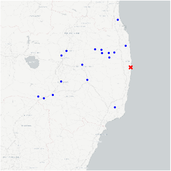
Figure 1: Sampled locations of the Cs-137 isotope, shown by a $\bullet$. The location of the power plant is shown by a $\times$.

The priors for $(\alpha,\beta,\sigma^{2})$ were used as in Section 2 with the following parameters: $a_{0}=0$, $s_{0}=0.1$, $b_{0}=0$, $q_{0}=0.01$, $d_{0}=0.1$, $e_{0}=0.1$. The fine grid $\Phi$ for estimating $\phi$ consists of 51 equally spaced points in $[0,0.1]$ and the coarse grid $\Phi_{K}$ consists of 7 equally spaced points in [0.002,0.098]. Algorithm 2 was used for estimation and prediction with particle size $N=1000$, MCMC size $L=500$ and Gibbs burn-in $B=100$.

Figure 2 shows the evolution of the parameter estimates in time. There is an apparent “jump” in the parameter estimates for $\beta$ and $\phi$ at around time $t=70$ after which the estimates become stable. A closer examination of the data reveals that this may be due to a lower trend after time 50 and to reduced sampling after time 40.

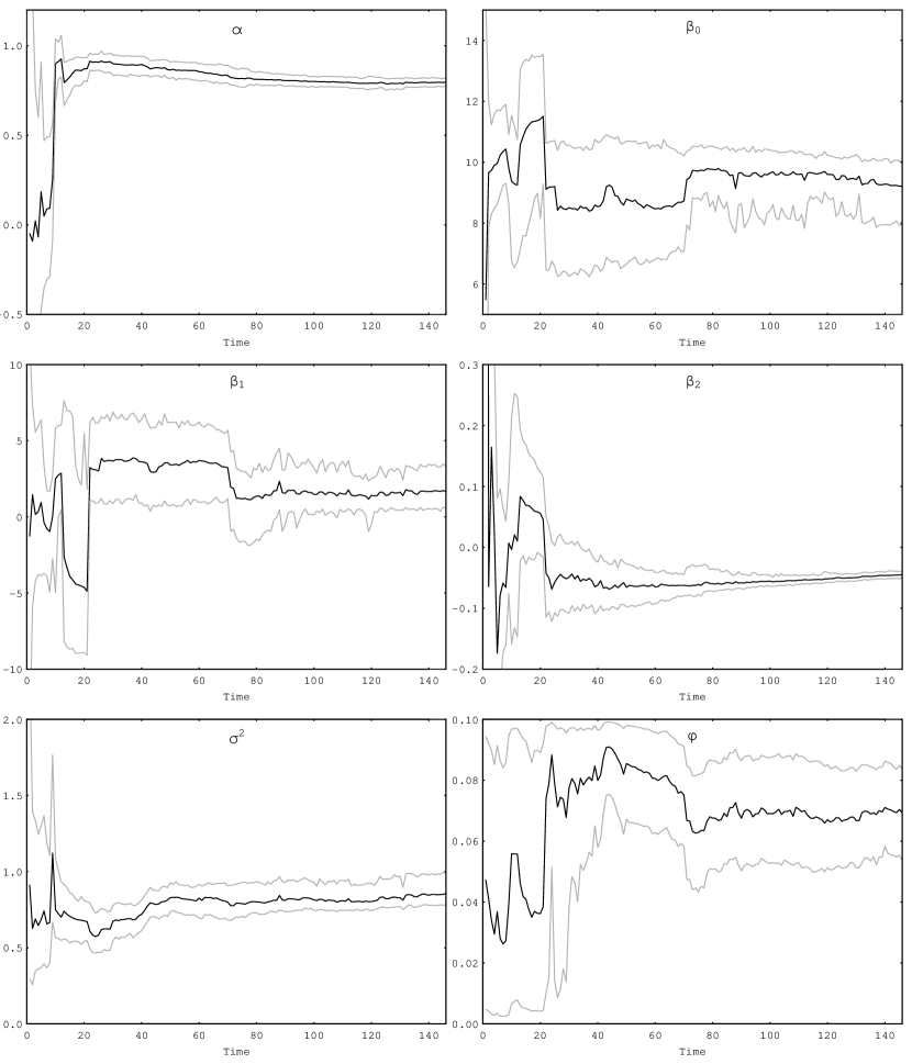
Figure 2: Estimates and 90% credible intervals for the parameters of the Fukushima power plant example.

Figure 3 shows the prediction at 2659 locations around the sampling area for selected times. To sample from the unmonitored locations we simulate from its conditional distribution given the samples at the monitored locations and the parameters, $p({\mathbf{x}}_{t}^{*}|{\mathbf{x}}_{0:t},\theta,\phi)$, where ${\mathbf{x}}_{t}^{*}$ is the value of the state process at the prediction locations. Figure 4 shows the standard deviation of our predictions. From the plots we can identify some radiation hot-spots and an apparent decrease of radiation over time.

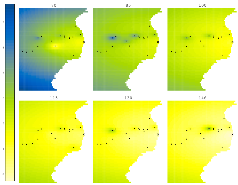
Figure 3: Predictions of the state process at different times for the Fukushima power plant example.

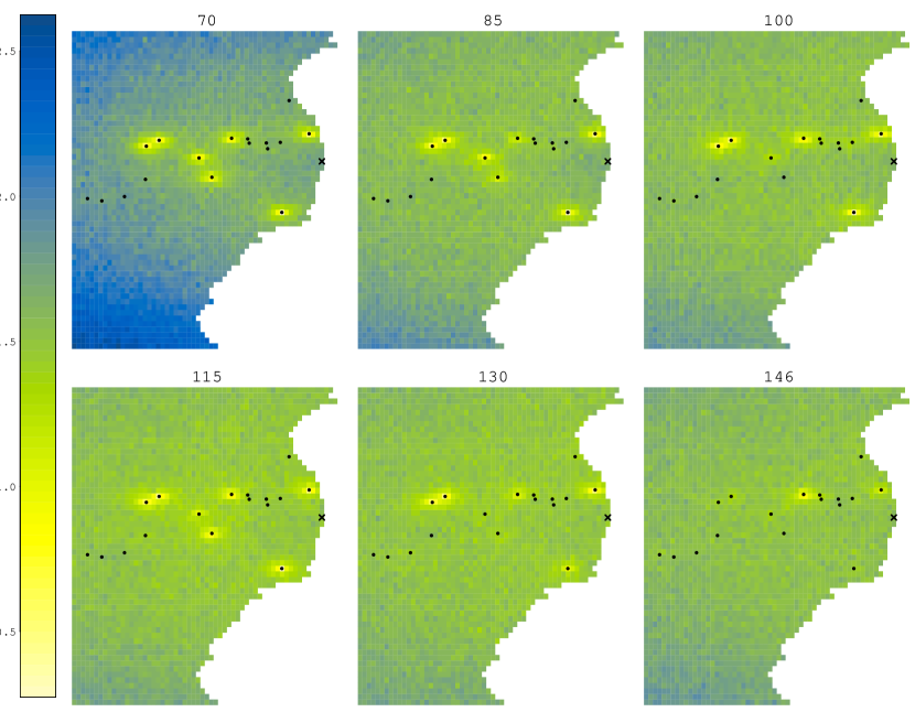
Figure 4: Prediction standard deviation of the state process at different times for the Fukushima power plant example.

5 Summary and discussion

In this paper we propose a method for online estimation and prediction of dynamic spatiotemporal processes. We consider a latent Gaussian autoregressive spatial process with data arriving sequentially in time with distribution from an exponential family conditional on the spatiotemporal process. Our model is expressed in terms of unknown parameters which are estimated along with the latent process within an empirical Bayes framework. We distinguish two types of parameters, the temporal parameters, which have a full conditional distribution that can be written in terms of sufficient quantities, and the spatial correlation parameters, which don’t. The spatial range parameter belongs to the latter type.

An algorithm is proposed for sampling from the filtering distribution of the spatiotemporal process and the posterior distribution of those parameters whose full conditional can be written in terms of sufficient quantities. These sufficient quantities are updated when new samples are taken for a fixed value of the range parameter, and because the filtering distribution can be skewed, we show how to use the skew-normal distribution to generate good candidate samples. The advantage of using sufficient quantities is that the storage requirements do not increase in time. These sufficient quantities depend on the spatial range parameter, thus, they are computed at a fixed set of values of that parameter across different times. Estimation of the range parameter is performed by maximizing the Bayes factors over this fixed set. The Bayes factors are estimated sequentially by importance sampling using the Monte Carlo samples.

Our method was compared against a typical offline MCMC method which samples from the posterior distribution of all parameters and the spatiotemporal field. We find that the distribution of the samples from our method matches the one obtained when the offline method is used. Finally, we demonstrate the application of our method on radiation measurements from a nuclear accident which can be used to assess the radiation risk in real time and provide helpful insight about its distribution.

Although the empirical Bayes estimation was applied to a single spatial correlation parameter, the theory is more general to allow more parameters to be estimated this way, e.g. a smoothness or a nugget parameter. For an application of this approach to the isotropic spatial model see roy16. On the other hand, when many parameters are included, the sampling and evaluation grids must be chosen carefully as a larger grid takes longer to compute.

Another extension of our model, is the use of a spatially-varying temporal autocorrelation parameter. Although this model allows us to capture the influence across spatial components, it becomes challenging to fit as there are more parameters to estimate.

Our model for the latent process assumes linear transition in time. Although not considered in this paper, it would be possible to apply the methodology to non-linear models using local linear approximations.

A potential research avenue is the application of this methodology to the dynamic spatiotemporal design problem, see e.g. WiRo1 incorporating parameter uncertainty in the design as well. Many interesting applications can be found in the point-process framework and it would be interesting to see how the suggested methodology performs in this case. Finally, the ideas of this paper can be applied to other models beyond the spatial framework.

6 Appendix

6.1 Proof of Lemma 1

We examine the limits for $i=1,\ldots,n$, of the ratio

$$\lim_{u\rightarrow\infty}\frac{p({\mathbf{x}}_{t}=\mu_{t}+u\mathbf{e}_{i}|{\mathbf{x}}_{t-1},{\mathbf{y}}_{t},\theta,\phi)}{p({\mathbf{x}}_{t}=\mu_{t}-u\mathbf{e}_{i}|{\mathbf{x}}_{t-1},{\mathbf{y}}_{t},\theta,\phi)},$$

where $\mu_{t}=G_{t}\beta+\alpha({\mathbf{x}}_{t-1}-G_{t-1}\beta)$ and $\mathbf{e}_{i}$ is a vector whose $i$th component is 1 and all other components are 0. If the limit is 0 or $\infty$, then the distribution is left or right skewed respectively.

Then, by the symmetry of the normal distribution around its mean,

$$\lim_{u\rightarrow\infty}\frac{p({\mathbf{x}}_{t}=\mu_{t}+u\mathbf{e}_{i}|{\mathbf{x}}_{t-1},{\mathbf{y}}_{t},\theta,\phi)}{p({\mathbf{x}}_{t}=\mu_{t}-u\mathbf{e}_{i}|{\mathbf{x}}_{t-1},{\mathbf{y}}_{t},\theta,\phi)} =\lim_{u\rightarrow\infty}\frac{p({\mathbf{y}}_{t}|{\mathbf{x}}_{t}=\mu_{t}+u\mathbf{e}_{i})p({\mathbf{x}}_{t}=\mu_{t}+u\mathbf{e}_{i}|{\mathbf{x}}_{t-1},\theta,\phi)}{p({\mathbf{y}}_{t}|{\mathbf{x}}_{t}=\mu_{t}-u\mathbf{e}_{i})p({\mathbf{x}}_{t}=\mu_{t}-u\mathbf{e}_{i}|{\mathbf{x}}_{t-1},\theta,\phi)}$$

$$=\lim_{u\rightarrow\infty}\frac{p({\mathbf{y}}_{t}|{\mathbf{x}}_{t}=\mu_{t}+u\mathbf{e}_{i})}{p({\mathbf{y}}_{t}|{\mathbf{x}}_{t}=\mu_{t}-u\mathbf{e}_{i})}$$

$$=\lim_{u\rightarrow\infty}\frac{p(y_{i,t}|x_{i,t}=\mu_{i,t}+u)}{p(y_{i,t}|x_{i,t}=\mu_{i,t}-u)},$$

where the last limit is either 0 or $\infty$ since the distribution of $y_{i,t}|x_{i,t}$ is skewed.

6.2 Proof of Theorem 1

The estimate of the sequential empirical Bayes factor, $\hat{B}_{1:t}(\phi;\tilde{\phi})$ in equation (12), depends on the associated sequential empirical Bayes factors, $\mathbf{b}_{t}=(b_{t}^{1},\ldots,b_{t}^{K})$, on the coarse grid for $\phi_{k}\in\Phi_{K}$. Consequently, we need to first establish the convergence of $\hat{b}_{t}^{k},\;k=1,\ldots,K$.

Because $\theta^{(k,l)}$ is drawn using Gibbs sampling, and because ${\mathbf{x}}_{t}^{(k,l)}$ is sampled by importance sampling conditioned on $\theta^{(k,l)}$, the sample $({\mathbf{x}}_{0:t}^{(k,l)},\theta^{(k,l)})$, $l=1,\ldots,L_{k}$ is a Harris ergodic Markov chain for each $k\in\{1,\ldots,K\}$ from the distribution $p({\mathbf{x}}_{0:t},\theta|{\mathbf{y}}_{1:t},\phi_{k})$.

Let $\lambda_{k}=L_{k}/\sum L_{k^{\prime}}$ and $\Lambda_{K}=\{\lambda_{1},\ldots,\lambda_{K}\}$. Then the concatenated sample $(x^{(k;l)}_{1:t},\theta^{(k;l)})$, $l=1,\ldots,L_{k}$, $k=1,\ldots,K$ is a Harris ergodic Markov chain from the mixture distribution with components the $p({\mathbf{x}}_{0:t},\theta|{\mathbf{y}}_{1:t},\phi_{k})$ and corresponding weights $\lambda_{k}$. The probability that the $(k,l)$th sample is drawn from the $k$th mixture component is given by

$$f({\mathbf{x}}_{0:t}^{(k,l)},\theta^{(k,l)}|{\mathbf{y}}_{1:t},\phi_{k})=\frac{\lambda_{k}p({\mathbf{x}}_{0:t}^{(k,l)},\theta^{(k,l)}|{\mathbf{y}}_{1:t},\phi_{k})}{p_{\text{{mix}}}({\mathbf{x}}_{0:t}^{(k,l)},\theta^{(k,l)}|{\mathbf{y}}_{1:t},\Phi_{K},\Lambda_{K})},$$

where $p_{\text{mix}}({\mathbf{x}}_{0:t},\theta|{\mathbf{y}}_{1:t},\Phi_{K},\Lambda_{K})$ denotes the mixture distribution of $p({\mathbf{x}}_{0:t},\theta|{\mathbf{y}}_{1:t},\phi_{k})$ for $k=1,\ldots,K$ with weights $\lambda_{k}$ defined in (11). Define the reverse logistic log-likelihood

$$\ell(\mathbf{b}_{t})=\sum_{k=1}^{K}\sum_{l=1}^{L_{k}}\log f({\mathbf{x}}_{0:t}^{(k,l)},\theta^{(k,l)}|{\mathbf{y}}_{1:t},\phi_{k}).$$ (16)

Then using similar arguments as in BuDo one may show that the maximizing argument of $\ell$, i.e. $\hat{\mathbf{b}}_{t}=\operatorname*{argmax}\ell(\mathbf{b}_{t})$ converges a.s. to the sequential empirical Bayes factors $\mathbf{b}_{t}$.

Next, observe that $\hat{B}_{1:t}(\phi;\tilde{\phi})$ can be written as

$$\sum_{k=1}^{K}\frac{1}{L_{k}}\sum_{l=1}^{L_{k}}\frac{\lambda_{k}p({\mathbf{x}}_{0:t}^{(k,l)}|\theta^{(k,l)},\phi)}{\sum_{k^{\prime}=1}^{K}\frac{\lambda_{k^{\prime}}}{\hat{b}^{k^{\prime}}_{t}}p({\mathbf{x}}_{0:t}^{(k,l)}|\theta^{(k,l)},\phi_{k^{\prime}})}\stackrel{{\scriptstyle\mbox{a.s.}}}{{\longrightarrow}}\sum_{k=1}^{K}\int\frac{\lambda_{k}p({\mathbf{x}}_{0:t}|\theta,\phi)}{\sum_{k^{\prime}=1}^{K}\frac{\lambda_{k^{\prime}}}{b^{k^{\prime}}_{t}}p({\mathbf{x}}_{0:t}|\theta,\phi_{k^{\prime}})}p({\mathbf{x}}_{0:t},\theta|{\mathbf{y}}_{1:t},\phi_{k})d({\mathbf{x}}_{0:t},\theta).$$ (17)

The right hand side of equation (17) equals

$$B_{1:t}(\phi;\tilde{\phi})\times\sum_{k=1}^{K}\int\frac{\lambda_{k}p({\mathbf{x}}_{0:t}|\theta,\phi)/p({\mathbf{y}}_{1:t}|\phi)}{\sum_{k^{\prime}=1}^{K}\lambda_{k^{\prime}}p({\mathbf{x}}_{0:t}|\theta,\phi_{k^{\prime}})/p({\mathbf{y}}_{1:t}|\phi_{k^{\prime}})}p({\mathbf{x}}_{0:t},\theta|{\mathbf{y}}_{1:t},\phi_{k})d({\mathbf{x}}_{0:t},\theta),$$ (18)

and multiplying and dividing by $p({\mathbf{y}}_{1:t}|{\mathbf{x}}_{0:t})p(\theta)$, one deduces that the finite sum of equation (18) equals 1. The proof is thus complete.

References

Sequential Empirical Bayes Method for Filtering Dynamic Spatiotemporal Processes
Web-based Supplementary Materials
Evangelos Evangelou¹   and Vasileios Maroulas^2
1 Department of Mathematical Sciences, University of Bath, Bath BA2 7AY, UK.

² Department of Mathematics, University of Tennessee, Knoxville, TN 37996, USA.

Simulation Results

The general setup of our simulations is as follows. The spatial dimension is the closed interval $[0,1]$ and the spatial sampling locations consist of $n=11$ equidistant points covering the spatial domain. The final sampling time is denoted by $T$. The latent spatiotemporal process ${\mathbf{x}}_{t}$ is simulated with constant mean $\beta=1$, autoregressive coefficient $\alpha=0.5$, and variance $\sigma^{2}=1$. The correlation between components of ${\mathbf{x}}_{t}$ is calculated using the exponential spatial correlation function, i.e.

$$\mathrm{Corr}({\mathbf{x}}_{i,t},{\mathbf{x}}_{j,t})=\exp(-d_{ij}/\phi),$$

where $d_{ij}$ stands for the distance between the $i$th and $j$th grid point and $\phi=0.4$ is the range parameter. At each time $t$ we simulate a response ${\mathbf{y}}_{t}$ conditioned on the simulated ${\mathbf{x}}_{t}$ such that $y_{i,t}\sim\mathrm{Poisson}(\tau e^{x_{i,t}})$ independently for each $i$, for given $\tau$.

For inference, the priors specified in (3) were used with $a_{0}=0$, $s_{0}=0.1$, $b_{0}=0$, $q_{0}=0.01$, $c_{0}=3$, and $r_{0}=1/3$. The fine grid $\Phi$ consisted of $J=41$ equidistant points between $\phi/2$ and $2\phi$, i.e. $\Phi=\{0.200,0.215,0.230,\ldots,0.800\}$ and the coarse grid to $\Phi_{K}=\{0.230,0.335,0.440,0.545,0.650,0.755\}$. The first element of $\Phi_{K}$ corresponds to $\tilde{\phi}$.

Algorithm 2 was run with Monte-Carlo sizes $L_{k}=L$ for $k=1,\ldots,K$ and Algorithm 1 with Gibbs iterations $L_{g}$ and particle size $N$.

1 Effect of the proposal distribution

In this section we compare the three choices of the proposal distribution discussed in the paper: (a) the Gaussian proposal; (b) the copula mean-only skewness correction; and (c) the copula mean-and-skewness correction.

The time dimension was $T=100$. We performed 30 simulations from the model with $\tau=1$. This model choice ensures that there is a substantial amount of skewness in the observations and will make the comparison between the three proposals more apparent. We measure the skewness of the approximation by computing the parameter $\delta^{2}=a^{2}/(1+a^{2})$ such that values of $\delta^{2}$ close to $1$ give large skewness and values close to $0$ give low skewness. In our simulations, the skew-normal parameter $\delta^{2}$ had an average value of 0.12 with the largest value being about 0.65.

The Monte-Carlo sizes were $L=100$, $N=100$, and $L_{\mathrm{g}}=50$.

For each time iteration we compute the effective sample size (ESS) for each method. Ideally we want $\mathrm{ESS}$ to be close to $N$ which will indicate that the proposal distribution generates good samples while a very low ESS would indicate degeneracy in the particles, which is not uncommon in high dimensions. Figure 1 shows a density plot for the distribution of the average ESS over the $L$ samples at each time iteration and for the 30 simulations (i.e, $30\times T$ values), expressed as a proportion of the total number of samples $N$ for each of the three proposal distributions. As shown in the figure, the uncorrected Gaussian proposal has a significantly lower ESS that the two corrected methods but the two skewness correction methods are very similar. Based on our results, and in the following, we consider the mean-only corrected proposal only.

Figure 1: Density plots of the average ESS divided by the total number of generaged particles for: Gausian proposal (solid); Gaussian with mean-only correction (dashed); copula with mean-and-skewness correction (dotted).

2 Comparison with the simplified Bayes factor estimator

The simplified Bayes factor estimator is given in (10). This estimator simulates conditioned on $\phi=\tilde{\phi}$ only and uses these samples to compute the Bayes factor estimate for all $\phi\in\Phi$. In this case the reverse logistic estimates are not needed. However, as we discuss in Remark 1, this can potentially introduce bias if the true $\phi$ is far from $\tilde{\phi}$.

In this section we compare the bias of the simplified Bayes factor estimator with the proposed estimator (12) for the same Poisson model used in Section 1 but with increased $L=500$ and $\tau=10$. We consider (10) with three different values of $\tilde{\phi}=0.395,0.500,0.710$, where the first value is very close to the true $\phi$, the second value is at the middle of the range of $\Phi$, and the third value is far from the true. The simplified Bayes factor estimator was tested on 30 simulated cases with burn-in $L_{\text{bi}}=50$, thinning $L_{\text{th}}=10$ and final sample size 3000. The average estimate over the 30 cases for each method was computed for each time point. This is plotted in Figure 2 for the parameters $\sigma^{2}$ and $\phi$. The estimation for the parameters $\alpha$ and $\beta$ did not show any obvious discrepancy.

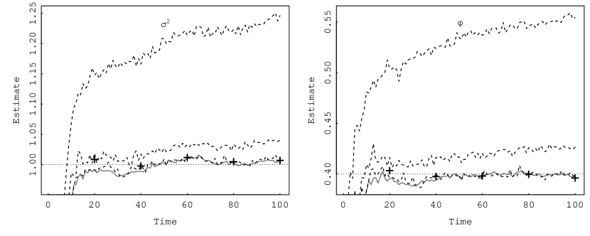
Figure 2: Average estimates for the parameters $\sigma^{2}$ and $\phi$ from the different Bayes factor estimators. The solid line is the mixed Bayes factor estimator (12). The dashed lines correspond to the simplified Bayes factor estimator (10) for $\tilde{\phi}=0.395,0.500,0.710$ from bottom to top. The average offline estimates are shown by $+$ and the true parameter value is shown by a horizontal line.

Our results verify that the simplified Bayes factor estimator is biased and this is more apparent when $\tilde{\phi}$ is far from the true $\phi$. Although the estimation for $\phi$ and $\sigma^{2}$ is biased, this does not seem to influence the estimation of $\alpha$ and $\beta$. This phenomenon has been observed elsewhere in the literature for the spatial-only case (see zhang2002estimation). Based on our results, the mixed Bayes factor estimator is recommended instead of the simplified one.

3 Estimation performance

In this section we assess the estimation performance of the proposed algorithm with the mean-only corrected proposal. We use the same setting as in Section 2 and the same 30 simulated data. We compare our estimates against an offline MCMC algorithm with the same Monte-Carlo sizes as Section 2. The offline MCMC algorithm uses Gibbs sampling for the parameters $\theta$ and a Metropolis-Hastings step to update $\phi$ and $x_{i,t}$, the $i$th component of ${\mathbf{x}}_{t}$ conditioned on everything else. The prior for $\phi$ was the exponential distribution with mean 0.4 and the Metropolis-Hastings step was selected for acceptance between 0.2 to 0.4. Convergence diagnostics of the MCMC output did not indicate any issues.

Because of the increasing computational time, we only ran the offline algorithm for selected time points $T_{i}=20,40,60,80,100$, where at each time only data up to $T_{i}$ were observed to make the results comparable with the online method.

In Figure 3 we plot the parameter estimates for each parameter in time for the online algorithm for each simulation and the distribution of the offline estimates from all simulations at the selected time points. It can be seen that the distributions from the two methods are very similar. In particular, the variability of our estimates reduces as we see more data and the bias is reduced which is a desirable property.

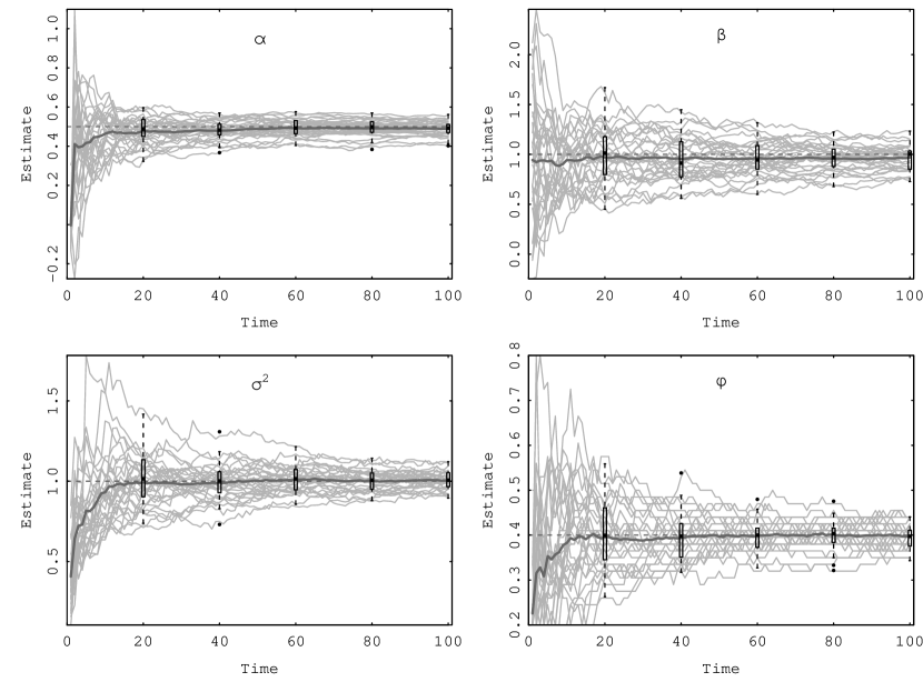
Figure 3: Comparison of estimates between the proposed online algorithm and the offline MCMC algorithm for the four parameters $\alpha$, $\beta$, $\sigma^{2}$, $\phi$. The light gray lines show the estimate for every simulation and the dark gray is the mean over all simulations. The boxplots show the distribution of the estimates using an offline MCMC algorithm with data available up to that time. The true parameter value is shown by a dashed line.

For each time iteration, the computing time for the sequential empirical Bayes algorithm was recorded, i.e. one iteration of Algorithm 2, and the average over the 30 simulations was taken. The average computing time is shown in Figure 4. It can be seen that the computing time does not increase in time as one would expect from an online algorithm.

Figure 4: Average computing time per time iteration for the sequential empirical Bayes algorithm across simulations. The computations were performed on computer with Intel Core i5-2500 3.30GHz CPU and 4Gb RAM.

Subsequently, the number of simulations was increased to 100, but in this case only the online algorithm was computed. This was to assess any potential bias in our method. The results from these simulations are shown in Figure 5 which show no apparent bias. On average, across all simulations, the four parameters are estimated accurately. Note the convergence of the estimates towards the true value and the reduction of uncertainty as more data are observed which demonstrates the suitability of our method. The sample variance of our estimates across simulations at each time point was calculated and its reciprocal was plotted against time. The plots corresponding to the four parameters are shown in Figure 6. It can be seen that the variability decreases linearly which indicates a reduction in the length of the posterior credible interval in the order of $1/\sqrt{t}$ as time $t$ increases.

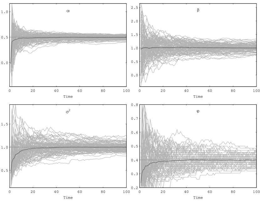
Figure 5: Estimates of $\alpha$, $\beta$, $\sigma^{2}$ and $\phi$ in that order across time. The dotted line shows the true parameter value, and the light gray lines represent the estimates corresponding to each simulation across time. The mean across all simulations is shown by a dark gray line.

Figure 6: Reciprocal of the sample variances across simulations of the estimates for $\alpha$, $\beta$, $\sigma^{2}$ and $\phi$ in that order across time. The dotted line indicates the linear rate increase in time for the reciprocal of the sample variance.

4 Simulation with longer time span

In this section we use simulated data to compare the proposed algorithm against an offline MCMC algorithm. In this example the data were simulated from the model of Section 2 but with final time increased to $T=1000$. Only one sample was generated in this example. The data were subsequently fitted using the proposed online algorithm and an offline MCMC smoothing algorithm. The priors for both methods were the same as in Section 1 and a Monte Carlo sizes were as in Section 2.

Figure 7 shows the function $\log B_{1:t}(\phi;\tilde{\phi})$ computed by the proposed online algorithm for selected values of $t$, along with the grids $\Phi_{K}$ and $\Phi$. The maximizer of this function is the estimate for $\phi$ at time $t$. Note that, as $t$ increases, the maximum of this function converges to the true value and the uncertainty is reduced. To derive a confidence interval we view $B_{1:t}(\phi;\tilde{\phi})$ as an unnormalized posterior pdf for $\phi$ and the corresponding cumulative sum is the unnormalized cumulative distribution function (cdf). We then approximate the corresponding quantiles by polynomial interpolation of $\phi$ against the normalized cdf.

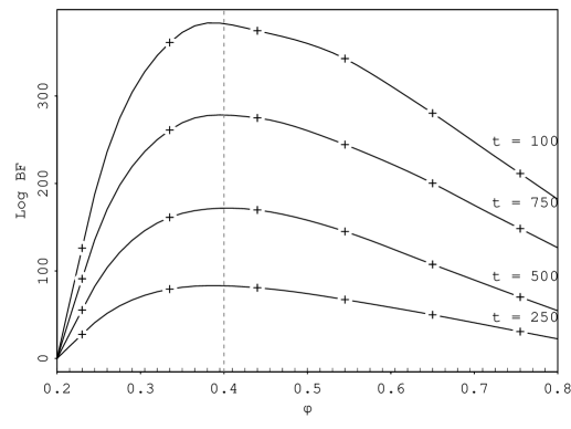
Figure 7: Logarithm of the Bayes factor, $\log B_{t}(\phi;\tilde{\phi})$, plotted against $\phi$ for different times. The true $\phi$ is shown by a vertical line. The coarse grid $\Phi_{K}$ is marked by $+$ on each line and the lines at the bottom show the fine grid $\Phi$.

The estimates (MC average for $\theta$, EB estimate for $\phi$) and 99% credible intervals (MC quantiles for $\theta$, polynomial interpolation for $\phi$) for each parameter using data ${\mathbf{y}}_{1:t}$ across $t$ are plotted in Figure 8. As shown in the figure, since both algorithms sample from the same posterior distribution, conditioned on ${\mathbf{y}}_{1:t}$, the estimates and credible intervals obtained between them are very similar and capture the true parameter values even for a longer time span.

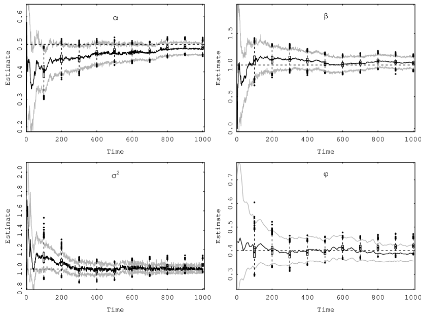
Figure 8: Parameter estimates across time using the proposed online algorithm (black lines) with 99% confidence intervals (light grey lines), and an offline algorithm (boxplots). The true parameter value is shown by a horizontal line.

References

References

{btSect}\btPrintCited

References

{btSect}\btPrintCited