TTP15-019, DESY 15-090, NIKHEF-2015-022
Exact N³LO results for $qq^{\prime}\to H+X$

Abstract

We compute the contribution to the total cross section for the inclusive production of a Standard Model Higgs boson induced by two quarks with different flavour in the initial state. Our calculation is exact in the Higgs boson mass and the partonic center-of-mass energy. We describe the reduction to master integrals, the construction of a canonical basis, and the solution of the corresponding differential equations. Our analytic result contains both Harmonic Polylogarithms and iterated integrals with additional letters in the alphabet.

PACS numbers: 14.80.Bn 12.38.B

1 Introduction

The precise determination of the properties of the recently discovered Higgs boson [1, 2] is among the main tasks of the upcoming run II of the CERN Large Hadron Collider (LHC). A crucial input to this enterprise is the total production cross section in gluon fusion.

Leading order (LO) contributions to $\sigma(pp\to H+X)$ were already computed by the end of the 1970s in Refs. [3, 4, 5, 6] and the next-to-leading order (NLO) QCD corrections have been available for almost 20 years [7, 8] including the exact dependence on the top quark mass (see also Ref. [9] for analytic results of the virtual corrections). NLO electroweak corrections have been computed in Ref. [10] and mixed QCD-electroweak corrections are considered in Ref. [11].

At LHC energies the NLO QCD corrections amount to 80-100% of the LO contributions which makes it mandatory to compute higher-order perturbative corrections. At the beginning of the century three groups independently evaluated the next-to-next-to-leading order (NNLO) corrections [12, 13, 14, 15] in the limit of an infinitely heavy top quark. Finite top quark mass effects, which have been investigated in Refs. [16, 17, 18, 19, 20, 21, 22], turn out to be at most of the order of 1%.

At next-to-next-to-next-to-leading order (N³LO) several groups have contributed building blocks to the total cross section. In Refs. [23, 24, 25] the effective Higgs-gluon coupling has been computed to four-loop accuracy. In preparation of the N³LO calculations the ${\cal O}(\epsilon)$ contributions to the NNLO master integrals have been computed in Refs. [22, 26] where $d=4-2\epsilon$ is the number of space-time dimensions in dimensional regularization. Results for the LO, NLO and NNLO partonic cross sections expanded up to order $\epsilon^{3}$, $\epsilon^{2}$ and $\epsilon^{1}$, respectively, have been published in Refs. [27, 28]. All contributions from convolutions of partonic cross sections with splitting functions, which are needed for the complete N³LO calculation, are provided in Refs. [27, 29, 28]. The full scale-dependence of the N³LO expression has been constructed in Ref. [28]. Three-loop ultraviolet counterterms needed for $\alpha_{s}$ [30, 31] and the operator in the effective Lagrangian [32] were computed long ago.

Within the effective theory, three-loop virtual corrections to the Higgs-gluon form factor have been obtained by two independent calculations [33, 34] (see also Ref. [35]). The single-soft current to two-loop order has been computed in Refs. [36, 37] which is an important ingredient to the two-loop corrections with one additional real radiation. The latter have been computed in Refs. [38, 39]. The single-real radiation contribution which originates from the square of one-loop amplitudes has been computed exactly in terms of the Higgs boson mass and the partonic center-of-mass energy in Refs. [40, 41]. The soft limit of the phase space integrals for Higgs boson production in association with two soft partons were computed in Refs. [42, 43], in the latter reference even to all orders in $\epsilon$. The triple-real contribution to the gluon-induced partonic cross section has been considered in Ref. [44] in the soft limit. In particular, a method has been developed which allows the expansion around the soft limit. A similar analysis for the double-real-virtual contributions has been published in Ref. [45].

The two leading terms in the threshold expansion for the complete N³LO total Higgs production cross section through gluon fusion have been presented in Refs. [42, 46, 47]. However, for physical applications more terms in the threshold expansion are necessary [46]. In fact, in Ref. [48] more than 30 expansion terms have been computed which is sufficient for all phenomenological applications. It is important to cross-check the result of Ref. [48]. In this paper we present the first step in this direction. In particular, results are obtained which are exact in the Higgs boson mass and the partonic center-of-mass energy.

Further activities concern the development of systematic approaches to compute the master integrals for $\sigma(pp\to H+X)$, see, e.g., Refs. [44, 40, 41, 49, 38].

Several groups have constructed approximate N³LO results for the total cross section taking into account information from the soft-gluon approximation and the high-energy limit [50, 51, 52, 53, 54, 55, 56].

In the following, we briefly outline the framework which we use for our calculation. In the limit of an infinitely heavy top quark the effective interaction of the Higgs boson with gluons is described by the Lagrange density

$${\cal L}_{Y,\rm eff} = -\frac{H^{0}}{4v^{0}}C_{1}^{0}(G_{\mu\nu}G^{\mu\nu})^{0}+{\cal L}_{QCD}^{(5)}\,,$$ (1)

where ${\cal L}_{QCD}^{(5)}$ is the usual QCD Lagrange density with five massless quarks, $H$ denotes the Higgs field, $v$ its vacuum expectation value and $C_{1}$ is the matching coefficient between the full and the effective theory. $G_{\mu\nu}$ is the gluonic field strength tensor constructed from fields and couplings already present in ${\cal L}_{QCD}^{(5)}$. The superscript “0” denotes the bare quantities. Note that the counterterms of $H^{0}/v^{0}$ are of higher order in the electroweak coupling constants.

The top quark mass enters the cross section via the matching coefficient $C_{1}$ whereas the quantities in the effective theory depend on

$$x = \frac{m_{h}^{2}}{\hat{s}}\,,$$ (2)

where $m_{h}$ is the Higgs boson mass and $\sqrt{\hat{s}}$ the partonic center-of-mass energy. For later convenience we also introduce the variable

$$y = 1-x\,.$$ (3)

At the partonic level several sub-processes initiated by quarks and gluons in the initial state have to be considered. The numerically most important but also technically most complicated contribution is the one with two gluons in the initial state. In the present paper we consider the subprocess $qq^{\prime}\to H+X$ at NNLO and N³LO. Its phenomenological impact is very small, but we use this process to demonstrate our method which leads to exact results in $x$ and avoids the high-order soft expansion.

For the calculation of the total cross section it is convenient to consider the imaginary part of the forward scattering amplitude $qq^{\prime}\to qq^{\prime}$. Sample Feynman diagrams contributing at NNLO and N³LO are shown in Fig. 1. To obtain the cross section all cuts involving the Higgs boson have to be computed which means that both three- and four-particle cuts have to be considered at N³LO. There are no two-particle cuts.

Figure 1: Sample Feynman diagrams for $qq^{\prime}\to qq^{\prime}$. The imaginary parts due to Higgs boson cuts provide the cross section for the process $qq^{\prime}\to H+X$ at NNLO and N³LO. Solid, curly and dashed lines represent quarks, gluons and Higgs bosons, respectively and blobs denote the effective Higgs-gluon couplings.

The remainder of the paper is organized as follows: In the next Section we discuss the reduction of the full set of integrals to master integrals and the construction of the canonical basis. For the latter integrals a system of differential equations is derived. The following two sections are dedicated to the evaluation of the initial conditions involving cuts of three (Section 3) and four (Section 4) particles. In Section 5 we introduce recursively defined iterated integrals which are needed for the analytic representation of the final result. The partonic cross section is discussed in Section 6 where analytic results are given. Finally we conclude in Section 7.

2 Reduction and canonical master integrals

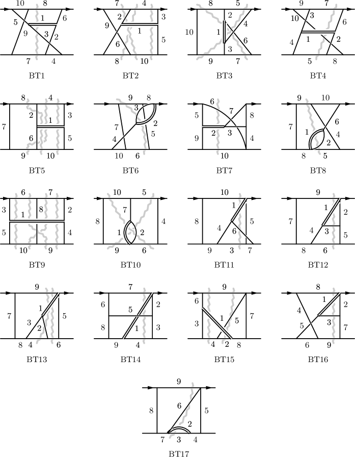
Figure 2: Graphical representations of the 17 three-loop integral families. Plain and double lines indicate massless propagators and the Higgs boson lines, respectively, and the wavy lines indicate the possible cuts.

We generate all two- and three-loop forward-scattering amplitudes for the process $q(p_{1})q^{\prime}(p_{2})\to q(p_{1})q^{\prime}(p_{2})$ involving a virtual Higgs boson with the help of qgraf [57] and process the output file to select the contributions which contain cuts through the Higgs boson line. This leads to 1 two-loop and 224 three-loop Feynman diagrams. At three-loop order the corresponding amplitudes can be mapped to 17 integral families which are shown in Fig. 2. For each of them reduction tables are generated using a combination of the publicly available program FIRE [58] and in-house programs, rows and TopoID [59], which implement the Laporta algorithm [60]. The use of rows and TopoID guarantees that all available symmetries are exploited which is important to minimize the number of master integrals. After completing the reduction for each family we obtain 332 master integrals. In our next step we minimize the number of integrals by simultaneously considering all families which leaves us with 111 master integrals, 108 of which are needed for the cross section. In the following we refer to this set of master integrals as “Laporta master integrals”.

Note that we have performed the calculation for general gauge parameter $\xi$ which drops out after relating master integrals from the different families. This constitutes a strong check on the correctness of our result.

For the evaluation of the master integrals we follow the ideas of Ref. [61] and construct a canonical basis which allows for a simple and straightforward solution of the corresponding differential equations (see Refs. [62, 63] for reviews on the use of differential equations for the computation of Feynman integrals). Whereas most of our calculation is automated to a high degree the construction of the canonical basis requires manual manipulations of each individual integral. We have applied several tricks described in the literature [64, 65, 66, 67, 68] and also follow the algorithm developed in Ref. [49] which allows the construction of canonical master integrals in coupled subsystems. In Ref. [69] an algorithm has been suggested which automates the construction of the canonical basis. However, a public implementation is not yet available.

In a canonical basis the differential equations have the form

$$\partial_{x}f(x,\epsilon) = \epsilon A(x)f(x,\epsilon)\,,$$ (4)

where $f(x,\epsilon)$ is a vector containing all canonical master integrals. In our case the matrix $A(x)$ can be written as

$$A(x) = \frac{a}{1-x}+\frac{b}{1+x}+\frac{c}{x}+\frac{d}{1+4x}+\frac{e}{x\sqrt{1+4x}}\,,$$ (5)

where $a,\ldots,e$ are constant matrices. The first three terms on the right-hand side of Eq. (5) lead to the well-known Harmonic Polylogarithms (HPLs) [70] (see Refs. [71, 72] for a convenient Mathematica implementation) in the solution of the master integrals. The fourth and fifth terms in Eq. (5) are only needed for the integral family BT3 as we will describe in detail in Section 5.

Besides the simple solution of the differential equations the canonical basis also has the advantage that for the initial conditions only the leading terms of order $y^{0}$ are needed in the soft limit. As a consequence, no explicit calculation is needed in case the first non-zero contribution of a canonical master integral is of ${\cal O}(y)$ or higher. In our calculation the boundary conditions are computed for Laporta master integrals. Afterwards the results are transformed to the canonical basis.

3 Three-particle cuts

The three-particle-cut contributions contain a one-loop sub-diagram. As our first step we represent the loop in terms of Mellin-Barnes integrals and perform the momentum integration. Afterwards in the soft limit all integrals are represented as phase space integrals of soft partons, which can be converted to integrals over energies and angles. These integrals are also calculable using Mellin-Barnes integrals. Hence, we obtain multifold Mellin-Barnes integral representations for each master integral in the soft limit. They are evaluated extending the method developed in Ref. [73] for the calculation of the three-loop static potential. The notation is mainly adopted from Ref. [44] where four-particle cuts have been considered. In this reference also a technique has been developed which transforms soft phase-space integrals to Mellin-Barnes integrals, which has been applied in Ref. [45] to three-particle phase space contributions. In contrast to Ref. [45] we do not apply the method of regions to compute the integrals.

Before describing the procedure in more detail we have to introduce some notation. We denote the external momenta by $p_{1},p_{2}$ and the light momenta involved in the cut by $p_{3},p_{4}$ and $p_{5}$, where $p_{5}$ will occur for the four-particle phase space integrals in Section 4. Loop momenta are denoted by $v_{i}$. According to Ref. [44] the scaling of the phase space momenta in the soft limit is given by $p_{i}\sim\sqrt{s}$ for $i=1,2$ and $p_{i}\sim y\sqrt{s}$ for $i=3,4$ and $5$ in the center-of-mass frame of the incoming quarks. We eliminate the momentum of the Higgs boson in favour of the momenta of the massless partons and define rescaled scalar products

$$s_{ij} = \begin{cases}\frac{(p_{i}-p_{j})^{2}}{sy},&i=1,2\text{ and }j>2\,,\\ \frac{(p_{i}+p_{j})^{2}}{sy^{2}}&i>2\text{ and }j>2\,.\end{cases}$$ (6)

Furthermore, we use the energies and angles parametrization

$$\frac{p_{1}}{\sqrt{s}} = \frac{1}{2}\beta_{1}=\frac{1}{2}(1,0_{d-2},1)^{\mathsf{T}}\,,$$

$$\frac{p_{2}}{\sqrt{s}} = \frac{1}{2}\beta_{2}=\frac{1}{2}(1,0_{d-2},-1)^{\mathsf{T}}\,,$$

$$\frac{p_{i}}{\sqrt{s}y} = \frac{1}{2}E_{i}\beta_{i}\quad\mbox{for}\quad i>2\,,$$ (7)

where $E_{i}$ parametrize the partons’ energies and $\beta_{i}$ their $d$-dimensional velocities. $0_{d-2}$ is an abbreviation for a sequence of $d-2$ zeros. For later convenience we also introduce $\beta_{ij}=\beta_{i}\cdot\beta_{j}$.

In the following we exemplify the individual steps of the algorithm on the integral

$$B_{9} = \mathrm{BT9}(1,1,1,0,1,0,1,0,1,1,0,0)$$ (8)

$$= \int{\rm d}\Phi_{3}^{s}\int\frac{{\rm d}^{d}v}{\left(2\pi\right)^{{d}}}\frac{N}{v^{2}(p_{1}{-}p_{3})^{2}(p_{1}{-}p_{3}{-}p_{4}+v)^{2}(p_{1}+p_{2}{-}p_{3}{-}p_{4}+v)^{2}}\,.$$

$N$ is a normalization factor given by

$$N = \frac{1}{2\pi}\left(\frac{(4\pi)^{2-\epsilon}}{\Gamma(1+\epsilon)}\right)^{3}\,,$$ (9)

where the factors $\Gamma(1+\epsilon)$ and $(4\pi)^{\epsilon}$ are introduced for convenience and ${\rm d}\Phi_{3}^{s}$ is the soft three-particle phase space measure which can be written as

$$\int{\rm d}\Phi_{3}^{s} = (2\pi)^{-5+4\epsilon}2^{-6+4\epsilon}s^{1-2\epsilon}y^{3-4\epsilon}\delta\left(1-\sum_{i=3}^{4}E_{i}\right)\prod_{i=3}^{4}E_{i}^{1-2\epsilon}\int{\rm d}E_{i}\int{\rm d}\Omega_{i}^{d-1}\,.$$ (10)

$\Omega_{i}^{d-1}$ is the $d$-dimensional solid angle.

The algorithm for the computation of the three-particle cut contribution is as follows:

1. Introduce a regularization parameter $\delta$ for the numerators. This is necessary to avoid terms $\Gamma(0)$ which otherwise could appear in step 5 below. We introduce $\delta$ to the exponent of the scalar products, namely, $\left(p_{i}+\cdots\right)^{2}\rightarrow\lim_{\delta\rightarrow 0}\left[\left(p_{i}+\cdots\right)^{2}\right]^{1+\delta}$.

2. Perform subloop integration and introduce Mellin-Barnes integrals.

   We (i) introduce Feynman parameters to combine propagators involving loop momenta, (ii) perform loop integration and (iii) introduce Mellin-Barnes variables to obtain a factorization of the Feynman variables [44] using the formula

   $$\frac{1}{(X+Y)^{\lambda}} = \frac{1}{\Gamma(\lambda)}\frac{1}{2\pi i}\int_{-i\infty}^{+i\infty}{\rm d}z\,\Gamma(\lambda+z)\Gamma(-z)\frac{Y^{z}}{X^{\lambda+z}}\,.$$ (11)

   In our example we obtain a one-fold Mellin-Barnes integral over $z_{1}$ which has the following form

   $$B_{9} = \int{\rm d}\Phi_{3}^{s}\int\frac{{\rm d}z_{1}}{2\pi i}\times$$

   $$\frac{2^{7-4\epsilon}\pi^{3-2\epsilon}\Gamma(-z_{1})\Gamma(z_{1}+1)\Gamma(-\epsilon)\Gamma(-z_{1}-\epsilon)\Gamma(z_{1}+\epsilon+1)}{(p_{1}{-}p_{3})^{2}(p_{1}+p_{2}{-}p_{3}{-}p_{4})^{-2z_{1}}(p_{1}{-}p_{3}{-}p_{4})^{2z_{1}+2\epsilon+2}\Gamma(1-2\epsilon)\Gamma^{3}(\epsilon+1)}\,.$$

3. Express the propagators in terms of velocities and energies, and take the soft limit, i.e., $y\to 0$.

   Using Eq. (6) we can replace the propagators in our examples $B_{9}$ as

   $$\frac{1}{(p_{1}{-}p_{3})^{2}} \rightarrow {-}\frac{2}{syE_{3}\beta_{13}}\,,$$

   $$\frac{1}{(p_{1}{-}p_{3}{-}p_{4})^{2+2z_{1}+2\epsilon}} \rightarrow \left(-\frac{1}{2}syE_{3}\beta_{13}-\frac{1}{2}syE_{4}\beta_{14}+\frac{1}{2}sy^{2}E_{3}E_{4}\beta_{34}\right)^{-z_{1}-\epsilon-1}\,,$$

   $$\frac{1}{(p_{1}+p_{2}{-}p_{3}{-}p_{4})^{-2z_{1}}} \rightarrow \left(\frac{1}{2}s{\beta_{12}}-\frac{1}{2}syE_{3}\beta_{13}-\frac{1}{2}syE_{4}\beta_{14}-\frac{1}{2}syE_{3}\beta_{23}\right.$$ (13)

   $$\mbox{}\left.-\frac{1}{2}syE_{4}\beta_{24}+\frac{1}{2}sy^{2}E_{3}E_{4}\beta_{34}\right)^{z_{1}}\,.$$

   To leading order in $y$ this becomes

   $$\frac{1}{(p_{1}{-}p_{3})^{2}} \rightarrow {-}\frac{2}{syE_{3}\beta_{13}}\,,$$

   $$\frac{1}{(p_{1}{-}p_{3}{-}p_{4})^{2+2z_{1}+2\epsilon}} \rightarrow \left(-\frac{1}{2}syE_{3}\beta_{13}-\frac{1}{2}syE_{4}\beta_{14}\right)^{-z_{1}-\epsilon-1}\,,$$

   $$\frac{1}{(p_{1}+p_{2}{-}p_{3}{-}p_{4})^{-2z_{1}}} \rightarrow \left(\frac{1}{2}s{\beta_{12}}\right)^{z_{1}}\,.$$ (14)

4. Introduce Mellin-Barnes variables to factor the $\beta_{ij}$ and $E$ dependence.

   In our example a further Mellin-Barnes parameter $z_{2}$ has to be introduced to decompose the sum on the r.h.s of Eq. (14). Afterwards, the energy integrations are trivial and we obtain

   $$B_{9} = \frac{2^{5\epsilon-2}\pi^{2\epsilon-2}s^{-3\epsilon-1}\Gamma(-\epsilon)}{\Gamma(1-2\epsilon)\Gamma^{3}(\epsilon+1)}\int\frac{{\rm d}z_{1}}{2\pi i}\int\frac{{\rm d}z_{2}}{2\pi i}(-1)^{z_{1}}y^{-z_{1}-5\epsilon+1}\Gamma(-z_{1})\Gamma(z_{1}+1)\Gamma(-z_{2})$$ (15)

   $$\mbox{}\times\frac{\Gamma(-z_{1}-\epsilon)\Gamma(z_{2}-2\epsilon+2)\Gamma(-z_{1}-z_{2}-3\epsilon)\Gamma(z_{1}+z_{2}+\epsilon+1)}{\Gamma(-z_{1}-5\epsilon+2)}$$

   $$\mbox{}\times\int{\rm d}\Omega_{3}^{{d-1}}\int{\rm d}\Omega_{4}^{{d-1}}\beta_{14}^{z_{2}}\beta_{13}^{-z_{1}-z_{2}-\epsilon-2}\,.$$

5. Convert angular integrations to Mellin-Barnes integrations. This is achieved by using repeatedly [74]

   $$\int\frac{{\rm d}\Omega_{i}^{{d-1}}}{\beta_{j_{1}i}^{\alpha_{1}}\cdots\beta_{j_{n}i}^{\alpha_{n}}}$$

   $$=\frac{2^{2-\sum_{m=1}^{n}\alpha_{m}-2\epsilon}\pi^{1-\epsilon}}{\prod_{k=1}^{n}{\Gamma}\left(\alpha_{k}\right)\Gamma\left(2-\sum_{m=1}^{n}\alpha_{m}-2\epsilon\right)}\Gamma\left(1-\sum_{m=1}^{n}\alpha_{m}-\epsilon-\sum_{k=1}^{n}\sum_{l=k}^{n}z_{kl}\right)$$

   $$\quad\times\int_{-i\infty}^{i\infty}\left[\prod_{k=1}^{n}\prod_{l=k}^{n}\frac{{\rm d}z_{kl}}{2\pi i}\Gamma\left(-z_{kl}\right)\beta_{j_{k}j_{l}}^{z_{kl}}\right]\left[\prod_{k=1}^{n}\Gamma\left(\alpha_{k}+\sum_{l=1}^{k}z_{lk}+\sum_{l=k}^{n}z_{kl}\right)\right]\,,$$ (16)

   in order to perform the $\Omega$ integrations.

   In the case of our example this leads to

   $$B_{9} = s^{-3\epsilon-1}\int\frac{{\rm d}z_{1}}{2\pi i}\int\frac{{\rm d}z_{2}}{2\pi i}y^{-z_{1}-5\epsilon+1}\cos(\pi z_{1})\Gamma(-z_{1})\Gamma(z_{1}+1)\Gamma(-z_{2})$$

   $$\mbox{}\times\frac{\Gamma(-\epsilon)\Gamma(-z_{1}-\epsilon)\Gamma(z_{2}-\epsilon+1)\Gamma(-z_{1}-z_{2}-2\epsilon-1)\Gamma(z_{1}+z_{2}+\epsilon+1)}{\Gamma(1-2\epsilon)\Gamma^{3}(\epsilon+1)\Gamma(-z_{1}-5\epsilon+2)}\,.$$

6. Simplification with Barnes’ Lemma.

   We use the routine DoAllBarnes[] of the package barnesroutines.m [75]. Before applying it, we convert the cosine to Gamma functions using either

   $$\cos(a) = \frac{\psi^{(0)}\left(1-\frac{a}{\pi}\right)}{\Gamma\left(1-\frac{a}{\pi}\right)\Gamma\left(\frac{a}{\pi}\right)}-\frac{\psi^{(0)}\left(\frac{a}{\pi}\right)}{\Gamma\left(1-\frac{a}{\pi}\right)\Gamma\left(\frac{a}{\pi}\right)}$$ (18)

   or

   $$\cos(a) = \frac{\pi}{\Gamma\left(\frac{1}{2}-\frac{a}{\pi}\right)\Gamma\left(\frac{1}{2}+\frac{a}{\pi}\right)}$$ (19)

   depending on whether half-integer arguments are present in the final expression or not. The latter should be avoided to arrive at simpler expressions.

7. Take the limit $\delta\rightarrow 0$ (if needed) and expand in $y$ and $\epsilon$.

   Using MBcontinue[] from the package MB.m [76], we can obtain Mellin-Barnes representations for the limits $\delta\to 0$ and $\epsilon\to 0$. To achieve this goal, we have slightly modified the code to prevent that $\log(y)$ terms appear.

   After that we expand the representation in $\delta$ and $\epsilon$ using MBexpand[], and in $y$ using MBasymptotics[] [77].

8. Further simplification of Mellin-Barnes integrals.

   We apply the following procedures iteratively:

   • MBapplyBarnes[]

   • DoAllBarnes[]

   • Simplification of the integration contours such that all integrals with the same number of Mellin-Barnes parameters have the same integration contours.

9. Conversion to nested sums and their evaluation.

   To achieve this, we first use the residue theorem to convert the integrals to sums. In case this step generates divergent infinite sums, we introduce a regulator $e^{\pm\sigma c_{i}z_{i}}$ in the integrand, where the $c_{i}$’s are properly chosen numbers, $\sigma$ is a regularization parameter, and the $z_{i}$’s are Mellin-Barnes parameters in the expression. For the evaluation of the sums, we use the summation program described in Ref. [73].

The final result for the integral $B_{9}$ reads

$$\frac{B_{9}}{s^{-3\epsilon-1}}= \frac{-\frac{1}{2}y^{2-5\epsilon}+\frac{1}{2}y^{2-4\epsilon}}{\epsilon^{3}}+\frac{-\frac{15}{4}y^{2-5\epsilon}+3y^{2-4\epsilon}}{\epsilon^{2}}+\frac{y^{2-5\epsilon}\left(\frac{11\zeta_{2}}{2}-\frac{175}{8}\right)+y^{2-4\epsilon}\left(14-6\zeta_{2}\right)}{\epsilon}$$

$$+y^{2-5\epsilon}\left(\frac{165\zeta_{2}}{4}+18\zeta_{3}-\frac{1875}{16}\right)+y^{2-4\epsilon}\left(-36\zeta_{2}-11\zeta_{3}+60\right)$$

$$+\epsilon\left[y^{2-5\epsilon}\left(\frac{1925\zeta_{2}}{8}+135\zeta_{3}-\frac{31\zeta_{4}}{8}-\frac{19375}{32}\right)\right.$$

$$\left.\qquad+y^{2-4\epsilon}\left(-168\zeta_{2}-66\zeta_{3}+\frac{105\zeta_{4}}{2}+248\right)\right]$$

$$+\epsilon^{2}\bigg{[}y^{2-5\epsilon}\left(-198\zeta_{3}\zeta_{2}+\frac{20625\zeta_{2}}{16}+\frac{1575\zeta_{3}}{2}-\frac{465\zeta_{4}}{16}+294\zeta_{5}-\frac{196875}{64}\right)$$

$$\qquad+y^{2-4\epsilon}\left(132\zeta_{3}\zeta_{2}-720\zeta_{2}-308\zeta_{3}+315\zeta_{4}-105\zeta_{5}+1008\right)\bigg{]}$$

$$+{\cal O}(\epsilon^{3})+{\cal O}(y^{3})\,,$$ (20)

where terms up to ${\cal O}(\epsilon^{6})$ have been computed. For brevity only terms up to order $\epsilon^{2}$ are shown.

We have used the described algorithm for all needed three-particle initial conditions with one exception: the result of the integral $\text{BT9}(1,0,1,0,1,1,1,0,1,1,0,0)$ where the lines $\{1,7,9\}$ are cut is taken over from Eq. (5.32) of Ref. [45].

As a cross check we have computed more integrals in the soft limit than actually necessary to fix the boundary conditions. Afterwards we have checked that the solution of the differential equation reproduces these additional terms.

Note that the algorithm described in this section can also be applied to the four-particle-cut contribution after applying obvious modifications. In this way we have cross checked most of our results, which have been obtained using the method which we describe in the next section.

4 Four-particle cuts

To compute the initial condition of the four-particle-cut contributions we closely follow the procedure described in Ref. [44]. For completeness we briefly repeat the individual steps in this section. The soft expansion of the four-particle cut integrals exhibit only one region, which is defined by the scaling in $y$ of the scalar products $s_{ij}$ defined in Eq. (6). Reversed unitarity [14] allows for an expansion in the limit $y\to 0$ of the Higgs boson propagator which in our parametrization is given by

$$y\left(\frac{1}{(p_{1}+p_{2}-p_{3}-p_{4}-p_{5})^{2}-x}\right)_{c}$$

$$=\sum_{k=0}^{\infty}\frac{y^{k}}{s}\left[-(s_{34}+s_{35}+s_{45})\right]^{k}\left(\frac{1}{\left(1+s_{13}+s_{23}+s_{14}+s_{24}+s_{15}+s_{25}\right)^{k+1}}\right)_{c}\,,$$ (21)

where the subscript “$c$” reminds that the propagator has to be cut. In the soft limit only the term $k=0$ is needed. The massless propagators of the quarks and gluons are expanded as a Taylor series in the limit $y\to 0$ as well. This yields shifts in indices of the propagators, which are removed by subsequently applying the Laporta algorithm [60] as implemented in FIRE [58] in the soft kinematics. We obtain eleven master integrals. Ten are given in Ref. [44] where analytical results are derived. The eleventh integral corresponds to the soft limit of $\text{BT1}(1,1,1,0,0,0,1,1,0,1,0,0)$ (cf. Fig. 2) which can be cast in the form

$$F_{11}(\epsilon) = \frac{1}{\Phi_{4}^{s}}\int\frac{{\rm d}\Phi_{4}^{s}}{(s_{13}+s_{14})(s_{14}+s_{15})}\,,$$ (22)

where $\Phi_{4}^{s}$ is defined in analogy to $\Phi_{3}^{s}$ in Eq. (10). In Ref. [44] this integral probably only contributes to higher orders in $y$ which is why it has not been discussed in that paper.

Following Ref. [44] we apply Eq. (11) to convert the sums in the denominator of Eq. (22) into products at the cost of introducing Mellin-Barnes integrals.

Introducing energies and angles in analogy to Eqs. (6) and (7) one can integrate the energies in terms of $\Gamma$ functions, such that the only non-trivial integrations are given by three integrations over solid-angles, each of the form of Eq. (16), which are turned into Mellin-Barnes integrals. Following this procedure, we arrive at a one-dimensional Mellin-Barnes integral

$$F_{11}(\epsilon) = \int_{-i\infty}^{+i\infty}\frac{{\rm d}z}{2\pi i}\frac{\Gamma(6-6\epsilon)\Gamma(-2\epsilon-z)\Gamma(-\epsilon-z)\Gamma(-z)\Gamma(1+z)\Gamma(1-\epsilon+z)}{\Gamma(4-6\epsilon)\Gamma^{2}(1-\epsilon)\Gamma(1-2\epsilon-z)}\,,$$ (23)

which we expand in $\epsilon$ and solve by applying the algorithm of Ref. [73]. As a final result we obtain

$$F_{11}(\epsilon) = 20\zeta_{2}+\epsilon(-54\zeta_{2}+140\zeta_{3})+\epsilon^{2}(36\zeta_{2}-378\zeta_{3}+600\zeta_{4})$$ (24)

$$\mbox{}+\epsilon^{3}(252\zeta_{3}+160\zeta_{2}\zeta_{3}-1620\zeta_{4}+1860\zeta_{5})$$

$$\mbox{}+\epsilon^{4}(-432\zeta_{2}\zeta_{3}+560\zeta_{3}^{2}+1080\zeta_{4}-5022\zeta_{5}+6420\zeta_{6})$$

$$\mbox{}+\epsilon^{5}(288\zeta_{2}\zeta_{3}-1512\zeta_{3}^{2}+4800\zeta_{3}\zeta_{4}+3348\zeta_{5}+960\zeta_{2}\zeta_{5}-17334\zeta_{6}+15240\zeta_{7})$$

$$\mbox{}+\mathcal{O}(\epsilon^{6})\,,$$

which we have checked numerically using the package MB.m [76]. We have also rederived the integrals $F_{2}(\epsilon),\dots,F_{10}(\epsilon)$ of Ref. [44]. It is interesting to note, that all coefficients of Eq. (24) are integers, an observation also made in Ref. [44] for the integrals $F_{2}(\epsilon),\dots,F_{10}(\epsilon)$.

For many master integrals, we computed more terms in the soft expansion than required to fix the integration constants. These terms could be compared to the expansion of the exact result and thus strong consistency checks are obtained.

Note that an alternative method to compute four-particle phase-space integrals in the soft limit has been developed in Ref. [78].

5 Iterated integrals beyond HPLs

The solution of 16 out of our 17 families can be expressed in terms of HPLs [70], however, for BT3 this is not possible. In fact, the differential equation of the canonical basis implies an alphabet for the iterated integrals which involves square roots. The letters are

$$\left\{\frac{1}{x},\frac{1}{1-x},\frac{1}{1+x},\frac{1}{1+4x},\frac{1}{x\sqrt{1+4x}}\right\}\,.$$ (25)

The master integrals in which the last two letters show up can be classified as having the common subtopology drawn in Fig. 3. The contributing integrals with this property are

$$\text{BT3}(1,0,0,1,1,1,1,1,1,0,0,0),$$

$$\text{BT3}(1,0,-1,1,1,1,1,1,1,0,0,0),$$

$$\text{BT3}(1,0,0,1,1,1,1,1,1,1,0,0),$$

$$\text{BT3}(1,1,1,1,1,1,1,1,1,0,0,0),$$

$$\text{BT3}(1,1,1,1,1,1,1,1,1,0,-1,0),$$

$$\text{BT3}(1,1,1,1,1,1,1,1,1,-1,0,0)\,.$$ (26)

In general the occurrence of square roots $\sqrt{x-x_{0}}$ can be anticipated by observing half-integers in the diagonalized form of the matrix residue at $x_{0}$, as shall be briefly explained in the following using the above example. Let us denote the system of differential equations for the integrals in Eq. (26) by $\partial_{x}\tilde{f}=\tilde{A}\tilde{f}$. We expand the matrix elements of $\tilde{A}$ in a Laurent series around $x_{0}=-1/4$ and take the coefficient of $(x-x_{0})^{-1}$, which is called the matrix residue. After diagonalization we obtain

$$\text{diag}(0,0,0,0,0,1/2-4\epsilon)\,.$$ (27)

In a next step we expand the element $\tilde{f}_{6}$ corresponding to the last entry of the diagonal matrix in a power series in $(x-x_{0})$ and obtain with the help of the differential equation $\partial_{x}\tilde{f}_{6}=(1/2-4\epsilon)\tilde{f}_{6}/(x-x_{0})$. Note that the occurrence of the half-integer prefactor on the right-hand side (for $\epsilon\rightarrow 0$) implies the occurrence of the square root $\sqrt{1+4x}$, which in the full solution may show up in coefficients and in the alphabet of iterated integrals.

The present calculation contrasts earlier ones encountering square root letters [79, 80, 81], where the occurrence of the square root is connected with the presence of massive two-particle or four-particle cuts in the integrals (cf. the connection of square root letters in iterated integrals with (inverse) binomial sums in [82], as well as calculations of Feynman diagrams involving (inverse) binomial sums in [83, 84, 85, 86]). Topology BT3, however, represents four-particle phase-space integrals with only one massive line in the final state.

Figure 3: Common subtopology of all the graphs in BT3 which generate square root letters.

The canonical differential equation can be solved, as usual, order-by-order in $\epsilon$. Afterwards the constants of integration have to be determined. This is done by expanding the generic solution in a generalized Taylor series expansion around $x=1$ and matching with a calculation in the soft limit. For the expansion one needs to extract the logarithmic part due to $\log(1-x)$. This can be done using the shuffle algebra, and making sure that $1/(1-x)$ never occurs in the rightmost index of the iterated integrals. As a result the iterated integrals either diverge like $\log(1-x)$ or are regular in the limit $x\rightarrow 1$. For the matching procedure one now only needs the $(1-x)^{0}$-order, i.e. the regular part evaluated at $x=1$, while logarithmic orders provide a cross check for the generic solution with the calculation of the boundary conditions.

In this way the canonical master integrals and hence the Laporta masters are expressed in terms of iterated integrals over the alphabet (25). For numerical evaluations, it is advantageous to modify the above alphabet to be

$$\left\{\frac{1}{x},\frac{1}{1-x},\frac{1}{1+x},\frac{1}{1+4x},\frac{1}{x}\left(\frac{1}{\sqrt{1+4x}}-1\right)\right\}\,,$$ (28)

so only one letter is singular as $x\rightarrow 0$.

The contributions to the single Higgs boson production amplitude do not span the full space of functions generated by the above alphabet. In fact the relevant iterated integrals involving the square root letter can be constructed from

$$f_{0}=\frac{1}{x}\,,\qquad f_{-1}=\frac{1}{1+x}\,,\qquad f_{s4}=\frac{1}{x}\left(\frac{1}{\sqrt{1+4x}}-1\right)\,.$$ (29)

For the treatment of algebraic relations and the series expansions of the iterated integrals with square root letters, the package HarmonicSums was used [87, 88, 89]. For the numerical implementation, the convergent series expansions around $x=0$ and $x=1$ are helpful, which are available once the letter $1/x$ is shuffled away from the rightmost position in the indices of the iterated integrals. Unfortunately in contrast to the case of HPLs [70, 90], the series expansion around $x=0$ has a radius of convergence of $1/4$, thus more terms in the expansions are needed.

The iterated integrals involving square root letters were implemented numerically in Mathematica, using series expansions for functions of weight $\leq$3 and up to twofold numerical integrals. In this way we are able to yield 10 good digits at the timescale of a second and below for the most complicated functions at weight 5.

6 Results

The total partonic cross section can be written as

$$\hat{\sigma} = C_{1}^{2}\tilde{\sigma}\,,$$ (30)

where $C_{1}^{2}$ and $\tilde{\sigma}$ are separately finite after renormalization [23] and the convolution of the lower-order cross sections with the splitting functions [27, 29, 28].

Our final result can be cast in the form

$$\tilde{\sigma}(qq^{\prime}\to H+X) = A\left[\left(\frac{\alpha_{s}}{\pi}\right)^{2}\tilde{\sigma}_{qq^{\prime}}^{(2)}+\left(\frac{\alpha_{s}}{\pi}\right)^{3}\tilde{\sigma}_{qq^{\prime}}^{(3)}\right]\,,$$ (31)

where $A=G_{F}\pi/(32\sqrt{2})$ and $\tilde{\sigma}_{qq^{\prime}}^{(2)}$ is given in Eq. (54) of Ref. [14] and $\tilde{\sigma}_{qq^{\prime}}^{(3)}$ reads after identifying renormalization and factorization scale with the Higgs boson mass (i.e. $\mu_{r}=\mu_{f}=m_{h}$)

$$\tilde{\sigma}_{qq^{\prime}}^{(3)}={} n_{l}\Biggl{[}\frac{1}{27}(x+2)^{2}H_{0}^{4}(x)+\frac{2}{243}\left(11x^{2}-40x+188\right)H_{0}^{3}(x)-\frac{4}{27}(x+2)^{2}\zeta_{2}H_{0}^{2}(x)$$

$$-\frac{1}{243}\left(772x^{2}+1156x-2213\right)H_{0}^{2}(x)-\frac{16}{9}(x-1)(x+3)H_{1}(x)H_{0}^{2}(x)$$

$$-\frac{1}{243}\left(3139x^{2}+5218x-7620\right)H_{0}(x)-\frac{40}{27}(x-1)(x+3)H_{1}^{2}(x)H_{0}(x)$$

$$+\frac{2}{27}\left(83x^{2}+264x+148\right)H_{0,1,1}(x)+\frac{4}{81}\left(107x^{2}+344x+164\right)H_{0,1}(x)H_{0}(x)$$

$$-\frac{32}{27}\left(x^{2}+x+4\right)\zeta_{2}H_{0}(x)-\frac{70}{81}(x-1)(13x+33)H_{1}(x)H_{0}(x)$$

$$-\frac{56}{27}(x+2)^{2}H_{0,0,1}(x)H_{0}(x)+\frac{40}{27}(x+2)^{2}H_{0,1,1}(x)H_{0}(x)-\frac{98}{135}(x+2)^{2}\zeta_{2}^{2}$$

$$-\frac{4}{27}(x+2)^{2}\zeta_{3}H_{0}(x)-\frac{8}{27}(x-1)(x+3)H_{1}^{3}(x)-\frac{1}{324}(x-1)(2549x+15343)$$

$$-\frac{1}{54}(x-1)(319x+771)H_{1}^{2}(x)-\frac{11}{27}(x+2)^{2}H_{0,1}^{2}(x)-\frac{8}{27}(x+2)^{2}\zeta_{2}H_{0,1}(x)$$

$$+\frac{2}{243}\left(215x^{2}-904x-1402\right)\zeta_{2}+\frac{2}{243}\left(469x^{2}+1840x-218\right)H_{0,1}(x)$$

$$-\frac{41}{486}(x-1)(169x+519)H_{1}(x)-\frac{4}{81}\left(119x^{2}+464x+260\right)H_{0,0,1}(x)$$

$$+\frac{56}{27}(x+2)^{2}H_{0,0,0,1}(x)+\frac{22}{27}(x+2)^{2}H_{0,1,0,1}(x)+\frac{16}{27}(x-1)(x+3)\zeta_{2}H_{1}(x)$$

$$+\frac{8}{9}(x+2)^{2}H_{0,1}(x)H_{0}^{2}(x)+\frac{8}{9}(x+2)^{2}H_{0,1,1,1}(x)+\frac{2}{81}\left(13x^{2}+184x+4\right)\zeta_{3}\Biggr{]}$$

$$+\frac{1}{729}\left(1064x^{3}-2853x^{2}+107433x-41149\right)H_{0}^{3}(x)-\frac{112}{27}(x+2)^{2}H_{0,1}(x)H_{0}^{3}(x)$$

$$-\frac{1}{27}\left(13x^{2}+135x+164\right)H_{0}^{4}(x)+\frac{4}{27}\left(29x^{2}-28x+28\right)\zeta_{2}H_{0}^{3}(x)$$

$$+\frac{8}{81}(x+1)(97x-294)H_{-1}(x)H_{0}^{3}(x)+\frac{7}{81}(x-1)(97x+285)H_{1}(x)H_{0}^{3}(x)$$

$$-\frac{1}{810}\left(175x^{2}-308x+216\right)H_{0}^{5}(x)-\frac{130}{27}(x-2)^{2}H_{0,-1}(x)H_{0}^{3}(x)$$

$$-\frac{356}{27}(x-3)(x+1)H_{-1}^{2}(x)H_{0}^{2}(x)+\frac{836}{27}(x-1)(x+3)H_{1}^{2}(x)H_{0}^{2}(x)$$

$$+\frac{1}{5832}\left(46480x^{3}-286656x^{2}+3753336x-1756017\right)H_{0}^{2}(x)$$

$$+\frac{35}{216}(118x+85)\sqrt{4x+1}H_{0}^{2}(x)-\frac{2}{81}\left(105x^{2}-1548x-1900\right)\zeta_{2}H_{0}^{2}(x)$$

$$-\frac{35}{54}\left(9x^{2}-2x-8\right)H_{s4}(x)H_{0}^{2}(x)+\frac{70}{9}(x-3)(x+1)H_{-1,s4}(x)H_{0}^{2}(x)$$

$$-\frac{35}{9}(x-6)xH_{0,s4}(1)H_{0}^{2}(x)-\frac{1}{81}\left(1083x^{2}-2556x-3046\right)H_{0,-1}(x)H_{0}^{2}(x)$$

$$+\frac{1}{486}(x+1)\left(80x^{2}+12889x-46117\right)H_{-1}(x)H_{0}^{2}(x)$$

$$-\frac{35}{9}(x-2)^{2}H_{0,-1,s4}(x)H_{0}^{2}(x)+\frac{1}{54}(x-1)\left(400x^{2}-1019x+35945\right)H_{1}(x)H_{0}^{2}(x)$$

$$-\frac{35}{9}(x-6)xH_{0,s4}(x)H_{0}^{2}(x)+\frac{1}{27}\left(1220x^{2}-4844x-7485\right)H_{0,1}(x)H_{0}^{2}(x)$$

$$+\frac{356}{27}(x-2)^{2}H_{0,-1,-1}(x)H_{0}^{2}(x)+\frac{140}{9}(x-3)(x+1)H_{0,s4}(1)H_{-1}(x)H_{0}(x)$$

$$-\frac{2}{27}\left(317x^{2}-1612x+212\right)H_{0,0,1}(x)H_{0}^{2}(x)-\frac{836}{27}(x+2)^{2}H_{0,1,1}(x)H_{0}^{2}(x)$$

$$+\frac{8}{9}\left(13x^{2}+31x+30\right)\zeta_{3}H_{0}^{2}(x)+\frac{592}{81}(x-3)(x+1)H_{-1}^{3}(x)H_{0}(x)$$

$$+\frac{3212}{81}(x-1)(x+3)H_{1}^{3}(x)H_{0}(x)-\frac{4}{135}\left(361x^{2}-1044x+36\right)\zeta_{2}^{2}H_{0}(x)$$

$$+\frac{28}{81}\log^{4}(2)(x-2)^{2}H_{0}(x)-\frac{2}{243}(x+1)\left(104x^{2}+1633x-7915\right)H_{-1}^{2}(x)H_{0}(x)$$

$$+\frac{224}{27}\text{Li}_{4}\left(\frac{1}{2}\right)(x-2)^{2}H_{0}(x)+\frac{14}{729}(x+1)\left(280x^{2}-1213x-5327\right)H_{-1}(x)H_{0}(x)$$

$$+\frac{1}{54}(x-1)\left(592x^{2}-847x+53333\right)H_{1}^{2}(x)H_{0}(x)-\frac{160}{27}(x-2)^{2}H_{0,-1}^{2}(x)H_{0}(x)$$

$$-\frac{1}{8748}\left(421040x^{3}-394707x^{2}-12461502x+7407221\right)H_{0}(x)$$

$$-\frac{1}{9}\left(79x^{2}-1028x-212\right)H_{0,1}^{2}(x)H_{0}(x)-\frac{56}{27}\log^{2}(2)(x-2)^{2}\zeta_{2}H_{0}(x)$$

$$-\frac{1}{243}\left(3008x^{3}-10503x^{2}+202176x-46836\right)\zeta_{2}H_{0}(x)$$

$$+\frac{35}{108}\sqrt{4x+1}(118x+85)H_{s4}(x)H_{0}(x)-\frac{35}{27}\left(9x^{2}-2x-8\right)H_{0,s4}(1)H_{0}(x)$$

$$-\frac{35}{9}(x-2)^{2}\zeta_{2}H_{0,s4}(1)H_{0}(x)+\frac{70}{9}(x-2)^{2}H_{-1,s4}(1)H_{0,s4}(1)H_{0}(x)$$

$$+\frac{140}{9}(x-3)(x+1)H_{-1,s4,s4}(x)H_{0}(x)-\frac{140}{9}(x-3)(x+1)H_{0,-1,s4}(x)H_{0}(x)$$

$$+\frac{70}{9}\log(2)(x-2)^{2}H_{0,0,s4}(1)H_{0}(x)-\frac{70}{9}(x-6)xH_{0,0,s4}(1)H_{0}(x)$$

$$+\frac{70}{9}(x-6)xH_{0,0,s4}(x)H_{0}(x)-\frac{70}{9}\log(2)(x-2)^{2}H_{0,s4,s4}(1)H_{0}(x)$$

$$+\frac{70}{9}(x-6)xH_{0,s4,s4}(1)H_{0}(x)-\frac{70}{9}(x-6)xH_{0,s4,s4}(x)H_{0}(x)$$

$$-\frac{70}{9}(x-2)^{2}H_{-1,0,0,s4}(1)H_{0}(x)-\frac{70}{9}(x-2)^{2}H_{-1,0,s4,s4}(1)H_{0}(x)$$

$$-\frac{70}{9}(x-2)^{2}H_{-1,s4,0,s4}(1)H_{0}(x)-\frac{70}{9}(x-2)^{2}H_{0,-1,s4,s4}(1)H_{0}(x)$$

$$-\frac{70}{9}(x-2)^{2}H_{0,-1,s4,s4}(x)H_{0}(x)+\frac{70}{9}(x-2)^{2}H_{0,0,-1,s4}(1)H_{0}(x)$$

$$+\frac{200}{9}(x-2)^{2}H_{0,0,-1}(x)H_{0}^{2}(x)-\frac{1}{81}(x-1)\left(908x^{2}+7916x-135025\right)H_{1}(x)H_{0}(x)$$

$$-\frac{35}{54}\left(9x^{2}-2x-8\right)H_{s4}(x)^{2}H_{0}(x)-\frac{4}{27}(x+1)(373x-1101)\zeta_{2}H_{-1}(x)H_{0}(x)$$

$$-\frac{8}{81}\left(306x^{2}-474x-497\right)H_{0,-1,-1}(x)H_{0}(x)-\frac{4}{27}(x-1)(307x+963)\zeta_{2}H_{1}(x)H_{0}(x)$$

$$+\frac{1}{243}\left(16x^{3}-5013x^{2}+4140x+28873\right)H_{0,-1}(x)H_{0}(x)-\frac{35}{9}(x-2)^{2}\zeta_{2}H_{0,s4,s4}(1)$$

$$+\frac{740}{27}(x-2)^{2}\zeta_{2}H_{0,-1}(x)H_{0}(x)+\frac{8}{9}(x+1)(27x-79)H_{-1}(x)H_{0,-1}(x)H_{0}(x)$$

$$-\frac{70}{9}(x-2)^{2}H_{0,s4}(1)H_{0,-1}(x)H_{0}(x)-\frac{8}{27}(x-1)(25x+117)H_{1}(x)H_{0,-1}(x)H_{0}(x)$$

$$+\frac{1}{243}\left(2960x^{3}+18009x^{2}-2034x+69166\right)H_{0,1}(x)H_{0}(x)$$

$$-\frac{448}{27}(x-2)^{2}H_{0,-1}(x)H_{0,1}(x)H_{0}(x)+\frac{8}{9}(x+1)(37x-113)H_{-1}(x)H_{0,1}(x)H_{0}(x)$$

$$+\frac{628}{27}(x+2)^{2}\zeta_{2}H_{0,1}(x)H_{0}(x)+\frac{2}{27}(x-1)(475x+1383)H_{1}(x)H_{0,1}(x)H_{0}(x)$$

$$+\frac{140}{9}(x-2)^{2}H_{0,0,-1,s4}(x)H_{0}(x)-\frac{16}{27}\left(43x^{2}-160x-111\right)H_{0,-1,1}(x)H_{0}(x)$$

$$-\frac{496}{27}(x-2)^{2}H_{0,0,-1,-1}(x)H_{0}(x)+\frac{4}{27}\left(81x^{2}-620x-112\right)H_{0,0,-1}(x)H_{0}(x)$$

$$+\frac{896}{27}(x-2)^{2}H_{0,0,-1,1}(x)H_{0}(x)-\frac{2}{81}\left(3996x^{2}-17088x-31681\right)H_{0,0,1}(x)H_{0}(x)$$

$$-52(x-2)^{2}H_{0,0,0,-1}(x)H_{0}(x)-\frac{16}{27}\left(43x^{2}-160x-111\right)H_{0,1,-1}(x)H_{0}(x)$$

$$+\frac{2}{27}\left(923x^{2}-8188x-6336\right)H_{0,1,1}(x)H_{0}(x)-\frac{592}{27}(x-2)^{2}H_{0,-1,-1,-1}(x)H_{0}(x)$$

$$+\frac{4}{9}\left(275x^{2}-820x+484\right)H_{0,0,0,1}(x)H_{0}(x)+\frac{896}{27}(x-2)^{2}H_{0,0,1,-1}(x)H_{0}(x)$$

$$+\frac{64}{27}\left(9x^{2}-20x+36\right)H_{0,1,0,-1}(x)H_{0}(x)+\frac{4}{27}\left(37x^{2}-838x+842\right)\zeta_{3}H_{0}(x)$$

$$+\frac{2}{9}\left(x^{2}-1340x-524\right)H_{0,1,0,1}(x)H_{0}(x)-\frac{3212}{27}(x+2)^{2}H_{0,1,1,1}(x)H_{0}(x)$$

$$+\frac{196}{27}\log(2)(x-2)^{2}\zeta_{3}H_{0}(x)-\frac{500}{9}(x-1)(x+3)\zeta_{2}H_{1}^{2}(x)$$

$$+\frac{1}{54}(x-1)\left(256x^{2}-237x+23559\right)H_{1}^{3}(x)+\frac{2}{135}\left(2269x^{2}-1338x+9038\right)\zeta_{2}^{2}$$

$$+\frac{35}{9}(x-6)xH_{0,s4}(1)^{2}+\frac{35}{9}(x-6)xH_{0,s4}(x)^{2}+\frac{872}{27}(x-3)(x+1)\zeta_{2}H_{-1}^{2}(x)$$

$$+\frac{1208}{81}(x-1)(x+3)H_{1}^{4}(x)-\frac{1}{2916}(x-1)\left(24448x^{2}+200029x-3186149\right)H_{1}^{2}(x)$$

$$+\frac{4}{81}\left(63x^{2}-6x+214\right)H_{0,-1}^{2}(x)-\frac{1}{27}\left(494x^{2}-5212x-4845\right)H_{0,1}^{2}(x)$$

$$+\frac{1}{26244}(x-1)\left(57136x^{2}-1139639x+29021665\right)+\frac{112}{27}\log^{2}(2)(x-3)(x+1)\zeta_{2}$$

$$-\frac{1}{1458}\left(8032x^{3}-239799x^{2}+1426872x-432084\right)\zeta_{2}-\frac{56}{81}\log^{4}(2)(x-3)(x+1)$$

$$-\frac{448}{27}\text{Li}_{4}\left(\frac{1}{2}\right)(x-3)(x+1)+\frac{35}{108}\sqrt{4x+1}(118x+85)H_{0,s4}(1)$$

$$+\frac{70}{9}(x-3)(x+1)\zeta_{2}H_{0,s4}(1)-\frac{35}{27}\left(9x^{2}-2x-8\right)H_{s4}(x)H_{0,s4}(1)$$

$$-\frac{140}{9}(x-3)(x+1)H_{-1,s4}(1)H_{0,s4}(1)+\frac{140}{9}(x-3)(x+1)H_{-1,s4}(x)H_{0,s4}(1)$$

$$-\frac{35}{108}\sqrt{4x+1}(118x+85)H_{0,s4}(x)+\frac{35}{27}\left(9x^{2}-2x-8\right)H_{s4}(x)H_{0,s4}(x)$$

$$-\frac{70}{9}(x-6)xH_{0,s4}(1)H_{0,s4}(x)+\frac{70}{9}(x-2)^{2}H_{0,s4}(1)H_{0,-1,s4}(1)$$

$$-\frac{70}{9}(x-2)^{2}H_{0,s4}(1)H_{0,-1,s4}(x)-\frac{140}{9}\log(2)(x-3)(x+1)H_{0,0,s4}(1)$$

$$-\frac{35}{27}\left(9x^{2}-2x-8\right)H_{0,0,s4}(1)+\frac{35}{27}\left(9x^{2}-2x-8\right)H_{0,0,s4}(x)$$

$$+\frac{140}{9}\log(2)(x-3)(x+1)H_{0,s4,s4}(1)+\frac{35}{27}\left(9x^{2}-2x-8\right)H_{0,s4,s4}(1)$$

$$-\frac{35}{27}\left(9x^{2}-2x-8\right)H_{0,s4,s4}(x)+\frac{140}{9}(x-3)(x+1)H_{-1,0,0,s4}(1)$$

$$-\frac{140}{9}(x-3)(x+1)H_{-1,0,0,s4}(x)+\frac{140}{9}(x-3)(x+1)H_{-1,0,s4,s4}(1)$$

$$-\frac{140}{9}(x-3)(x+1)H_{-1,0,s4,s4}(x)+\frac{140}{9}(x-3)(x+1)H_{-1,s4,0,s4}(1)$$

$$-\frac{140}{9}(x-3)(x+1)H_{-1,s4,0,s4}(x)+\frac{140}{9}(x-3)(x+1)H_{0,-1,s4,s4}(1)$$

$$-\frac{140}{9}(x-3)(x+1)H_{0,-1,s4,s4}(x)-\frac{140}{9}(x-3)(x+1)H_{0,0,-1,s4}(1)$$

$$+\frac{140}{9}(x-3)(x+1)H_{0,0,-1,s4}(x)-\frac{70}{9}(x-2)^{2}H_{0,-1,0,s4,s4}(1)$$

$$+\frac{70}{9}(x-2)^{2}H_{0,-1,0,s4,s4}(x)-\frac{70}{9}(x-2)^{2}H_{0,-1,s4,0,s4}(1)$$

$$+\frac{70}{9}(x-2)^{2}H_{0,-1,s4,0,s4}(x)+\frac{140}{9}(x-2)^{2}H_{0,0,-1,0,s4}(1)$$

$$-\frac{140}{9}(x-2)^{2}H_{0,0,-1,0,s4}(x)-\frac{140}{9}(x-2)^{2}H_{0,0,-1,s4,s4}(1)$$

$$+\frac{140}{9}(x-2)^{2}H_{0,0,-1,s4,s4}(x)+\frac{140}{3}(x-2)^{2}H_{0,0,0,-1,s4}(1)$$

$$-\frac{140}{3}(x-2)^{2}H_{0,0,0,-1,s4}(x)+\frac{70}{3}(x-2)^{2}H_{0,0,0,s4,-1}(1)$$

$$-\frac{70}{3}(x-2)^{2}H_{0,0,0,s4,-1}(x)+\frac{70}{9}(x-2)^{2}H_{0,0,s4,0,-1}(1)$$

$$-\frac{70}{9}(x-2)^{2}H_{0,0,s4,0,-1}(x)-\frac{4}{27}(x+1)\left(4x^{2}+400x-1489\right)\zeta_{2}H_{-1}(x)$$

$$+\frac{140}{9}(x-3)(x+1)H_{0,0,s4}(1)H_{-1}(x)-\frac{140}{9}(x-3)(x+1)H_{0,s4,s4}(1)H_{-1}(x)$$

$$-\frac{1}{1458}(x-1)\left(52112x^{2}-42806x-2393137\right)H_{1}(x)+\frac{64}{3}(x-2)^{2}H_{0,1}(x)H_{0,1,-1}(x)$$

$$-\frac{8}{243}(x-1)\left(418x^{2}-2777x+32665\right)\zeta_{2}H_{1}(x)+\frac{70}{9}(x-2)^{2}H_{0,0,s4}(x)H_{0,-1}(x)$$

$$+\frac{8}{27}\left(50x^{2}-131x-165\right)\zeta_{2}H_{0,-1}(x)-\frac{592}{27}(x-3)(x+1)H_{-1}^{2}(x)H_{0,-1}(x)$$

$$-\frac{14}{729}(x+1)\left(280x^{2}-1213x-5327\right)H_{0,-1}(x)-\frac{70}{9}(x-2)^{2}H_{0,0,s4}(1)H_{0,-1}(x)$$

$$-\frac{140}{9}(x-3)(x+1)H_{0,s4}(1)H_{0,-1}(x)+\frac{70}{9}(x-2)^{2}H_{0,s4,s4}(1)H_{0,-1}(x)$$

$$+\frac{4}{243}(x+1)\left(104x^{2}+1633x-7915\right)H_{-1}(x)H_{0,-1}(x)$$

$$-\frac{64}{3}(x-3)(x+1)H_{-1}^{2}(x)H_{0,1}(x)+\frac{68}{27}(x-1)(x+3)H_{1}^{2}(x)H_{0,1}(x)$$

$$+\frac{1}{1458}\left(21656x^{3}-106251x^{2}-38232x+710568\right)H_{0,1}(x)$$

$$-\frac{4}{81}\left(2373x^{2}-4638x-8990\right)\zeta_{2}H_{0,1}(x)+\frac{256}{27}(x-2)^{2}H_{0,1}(x)H_{0,0,-1}(x)$$

$$-\frac{2}{243}(x+1)\left(32x^{2}-5567x+18887\right)H_{-1}(x)H_{0,1}(x)$$

$$-\frac{8}{243}(x-1)\left(14x^{2}+194x-355\right)H_{1}(x)H_{0,1}(x)+\frac{4}{81}\left(51x^{2}-430\right)H_{0,-1}(x)H_{0,1}(x)$$

$$-\frac{4}{243}(x+1)\left(104x^{2}+1633x-7915\right)H_{0,-1,-1}(x)-\frac{872}{27}(x-2)^{2}\zeta_{2}H_{0,-1,-1}(x)$$

$$+\frac{1184}{27}(x-3)(x+1)H_{-1}(x)H_{0,-1,-1}(x)+\frac{592}{27}(x-2)^{2}H_{0,-1}(x)H_{0,-1,-1}(x)$$

$$+\frac{64}{3}(x-2)^{2}H_{0,1}(x)H_{0,-1,-1}(x)+\frac{2}{243}(x+1)\left(32x^{2}-5567x+18887\right)H_{0,-1,1}(x)$$

$$+\frac{128}{3}(x-3)(x+1)H_{-1}(x)H_{0,-1,1}(x)-\frac{32}{3}(x-2)^{2}H_{0,-1}(x)H_{0,-1,1}(x)$$

$$-\frac{1}{243}\left(112x^{3}+2943x^{2}-24948x+11629\right)H_{0,0,-1}(x)-\frac{1048}{27}(x-2)^{2}\zeta_{2}H_{0,0,-1}(x)$$

$$+\frac{140}{9}(x-2)^{2}H_{0,s4}(1)H_{0,0,-1}(x)+\frac{32}{27}(x+1)(4x-15)H_{-1}(x)H_{0,0,-1}(x)$$

$$+\frac{16}{27}(x-1)(25x+117)H_{1}(x)H_{0,0,-1}(x)-\frac{8}{3}(x-2)^{2}H_{0,-1}(x)H_{0,0,-1}(x)$$

$$-\frac{1}{243}\left(4112x^{3}+17235x^{2}+8928x-11415\right)H_{0,0,1}(x)$$

$$+\frac{16}{27}\left(83x^{2}-316x+68\right)\zeta_{2}H_{0,0,1}(x)-\frac{16}{9}(x+1)(7x-23)H_{-1}(x)H_{0,0,1}(x)$$

$$-\frac{4}{27}(x-1)(407x+1179)H_{1}(x)H_{0,0,1}(x)+\frac{128}{3}(x-3)(x+1)H_{-1}(x)H_{0,1,-1}(x)$$

$$+\frac{4}{81}\left(529x^{2}-2060x+620\right)H_{0,1}(x)H_{0,0,1}(x)+\frac{176}{27}(x-2)^{2}H_{0,-1}(x)H_{0,0,1}(x)$$

$$+\frac{2}{243}(x+1)\left(32x^{2}-5567x+18887\right)H_{0,1,-1}(x)-\frac{32}{3}(x-2)^{2}H_{0,-1}(x)H_{0,1,-1}(x)$$

$$+\frac{1}{243}\left(3600x^{3}+28827x^{2}-50220x+145505\right)H_{0,1,1}(x)+\frac{500}{9}(x+2)^{2}\zeta_{2}H_{0,1,1}(x)$$

$$+\frac{128}{3}(x-3)(x+1)H_{-1}(x)H_{0,1,1}(x)+\frac{8}{27}(x-1)(x+3)H_{1}(x)H_{0,1,1}(x)$$

$$-\frac{64}{3}(x-2)^{2}H_{0,-1}(x)H_{0,1,1}(x)+\frac{2}{27}\left(27x^{2}+1836x+812\right)H_{0,1}(x)H_{0,1,1}(x)$$

$$-\frac{1184}{27}(x-3)(x+1)H_{0,-1,-1,-1}(x)-\frac{128}{3}(x-3)(x+1)H_{0,-1,-1,1}(x)$$

$$-\frac{128}{3}(x-3)(x+1)H_{0,-1,1,-1}(x)-\frac{128}{3}(x-3)(x+1)H_{0,-1,1,1}(x)$$

$$-\frac{32}{27}(x+1)(4x-15)H_{0,0,-1,-1}(x)-\frac{8}{81}\left(75x^{2}+840x-718\right)H_{0,0,-1,1}(x)$$

$$-\frac{2}{27}\left(179x^{2}-2740x+22\right)H_{0,0,0,-1}(x)+\frac{2}{27}\left(555x^{2}-5808x-11551\right)H_{0,0,0,1}(x)$$

$$-\frac{8}{81}\left(75x^{2}+840x-718\right)H_{0,0,1,-1}(x)-\frac{128}{3}(x-3)(x+1)H_{0,1,-1,-1}(x)$$

$$-\frac{128}{3}(x-3)(x+1)H_{0,1,-1,1}(x)-\frac{4}{81}\left(201x^{2}+552x-1132\right)H_{0,1,0,-1}(x)$$

$$+\frac{2}{81}\left(2847x^{2}-13308x-17566\right)H_{0,1,0,1}(x)-\frac{128}{3}(x-3)(x+1)H_{0,1,1,-1}(x)$$

$$+\frac{2}{27}\left(1905x^{2}-9008x-8556\right)H_{0,1,1,1}(x)-\frac{1184}{27}(x-2)^{2}H_{0,-1,0,-1,-1}(x)$$

$$+\frac{32}{3}(x-2)^{2}H_{0,-1,1,0,-1}(x)-\frac{2368}{27}(x-2)^{2}H_{0,0,-1,-1,-1}(x)$$

$$+\frac{568}{27}(x-2)^{2}H_{0,0,-1,0,-1}(x)+\frac{128}{3}(x-2)^{2}H_{0,0,-1,1,1}(x)$$

$$+\frac{568}{9}(x-2)^{2}H_{0,0,0,-1,-1}(x)-48(x-2)^{2}H_{0,0,0,-1,1}(x)$$

$$+\frac{512}{9}(x-2)^{2}H_{0,0,0,0,-1}(x)-\frac{8}{27}\left(577x^{2}-1580x+1296\right)H_{0,0,0,0,1}(x)$$

$$-48(x-2)^{2}H_{0,0,0,1,-1}(x)-\frac{16}{27}\left(59x^{2}-108x+236\right)H_{0,0,1,0,-1}(x)$$

$$-\frac{4}{27}\left(295x^{2}-2996x-316\right)H_{0,0,1,0,1}(x)-\frac{128}{3}(x-2)^{2}H_{0,0,1,1,-1}(x)$$

$$+\frac{32}{3}(x-2)^{2}H_{0,1,-1,0,-1}(x)-\frac{64}{3}(x-2)^{2}H_{0,1,-1,0,1}(x)$$

$$-\frac{512}{27}\left(x^{2}+4\right)H_{0,1,0,0,-1}(x)+\frac{4}{81}\left(71x^{2}+4460x+1780\right)H_{0,1,0,0,1}(x)$$

$$-\frac{64}{3}(x-2)^{2}H_{0,1,0,1,-1}(x)-\frac{2}{27}\left(151x^{2}+5788x+2716\right)H_{0,1,0,1,1}(x)$$

$$+\frac{64}{3}(x-2)^{2}H_{0,1,1,0,-1}(x)-\frac{2}{27}\left(61x^{2}+1972x+948\right)H_{0,1,1,0,1}(x)$$

$$-\frac{4832}{27}(x+2)^{2}H_{0,1,1,1,1}(x)+\frac{16}{27}\left(31x^{2}+354x+58\right)\zeta_{5}$$

$$-\frac{392}{27}\log(2)(x-3)(x+1)\zeta_{3}-\frac{2}{243}\left(848x^{3}+819x^{2}+102132x-25745\right)\zeta_{3}$$

$$-\frac{2}{27}\left(147x^{2}+2564x+236\right)\zeta_{2}\zeta_{3}-\frac{35}{3}(x-2)^{2}H_{0,s4}(1)\zeta_{3}$$

$$-\frac{4}{27}(x+1)(445x-1329)H_{-1}(x)\zeta_{3}-\frac{32}{27}(x-1)(76x+249)H_{1}(x)\zeta_{3}$$

$$+\frac{296}{9}(x-2)^{2}H_{0,-1}(x)\zeta_{3}+\frac{424}{9}(x+2)^{2}H_{0,1}(x)\zeta_{3}\,.$$ (32)

A computer-readable version of this equation can be obtained from [91]. In Eq. (32) $n_{l}=5$ denotes the number of massless quarks and $\zeta_{n}$ stands for Riemann’s zeta function evaluated at $n$. $H_{\vec{a}}(x)$ where $\vec{a}$ only has the elements $0$ and $\pm 1$ denote HPLs [70]. In case $\vec{a}$ contains also $s4$ the corresponding function refers to the iterated integral with square-root element introduced in Eq. (29) of Section 5. In Eq. (32) we observe iterated integrals up to weight 5.

Some of the iterated integrals in Eq. (32), which are evaluated for $x=1$, can be transformed to combinations of Riemann zeta functions. However, we prefer to leave $H_{\vec{a}}(1)$ since these terms disappear by construction in case Eq. (32) is evaluated for $x=1$.

The square root letter occurring in the result for the topology BT3 has already been introduced in Ref. [82], where it was named $f_{w_{14}}$. The corresponding iterated integrals occurred in the context of the calculation of three-loop contributions to massive operator matrix elements of Ref. [92]. Interestingly, using the substitution $x\rightarrow(1-x^{\prime})/x^{\prime\,2}$, the integrals involving $f_{s4}$ in Eq. (32) can be brought into the form of cyclotomic polylogarithms (cf. Ref. [93]) and can thus be represented as Goncharov polylogarithms [94] with the sixth root of unity appearing in the indices, more precisely with the alphabet $\{1,0,(-1)^{1/3}\}$. Furthermore, all functions without a letter $(-1)$ can be reduced to HPLs at the cost of a more complicated argument and an increase of the number of terms. In this representation the constants introduced via matching at $x=1$ are cyclotomic/multiple polylogarithms evaluated at the reciprocal of the golden ratio $x^{\prime}=(\sqrt{5}-1)/2$. Nevertheless, since the $H_{\ldots s4\ldots}$ are by construction real and since their numerical implementation is straightforward we decided not to rewrite the expression in Eq. (32).

In Ref. [46] the second term in the threshold expansion for the N³LO corrections to Higgs boson production has been computed. Furthermore, for all contributing partonic channels the exact dependence on $x$ is provided for the coefficients of the leading logarithms in $\log(1-x)$. In Eq. (32) only (some of) the HPLs are divergent in the limit $x\to 1$ since in the iterated integrals involving $s4$ the letter $1/(1-x)$ is absent. After extracting the logarithmic divergencies of the HPLs we find full agreement with the results given in Eqs. (2.26) and (2.27) of [46] for the coefficients of the $\log^{3}(1-x)$ and $\log^{4}(1-x)$ contribution, respectively.

7 Conclusions

In this paper we have computed a contribution to the third-order partonic cross section for Higgs boson production in gluon fusion, namely the sub-process initiated by two quarks with different flavour. The numerical impact of this contribution is small. However, we have obtained analytic results retaining the exact dependence on the Higgs boson mass and the partonic center-of-mass energy. This constitutes a new result since to date only an expansion around the soft limit has been presented in the literature. Our findings constitute an important step towards an exact result of all third-order contributions to the Standard Model Higgs boson production.

In the course of our calculation we have mapped all contributing amplitudes to 17 integral families. For each family we have constructed a canonical basis and derived the corresponding system of differential equations. After evaluating the three- and four-particle cut initial conditions the differential equations could be solved in terms of HPLs in all integral families except one, which required additional letters in the alphabet of the iterated integrals.

References

• [1] G. Aad et al. [ATLAS Collaboration], Phys. Lett. B 716 (2012) 1 [arXiv:1207.7214 [hep-ex]].
• [2] S. Chatrchyan et al. [CMS Collaboration], Phys. Lett. B 716 (2012) 30 [arXiv:1207.7235 [hep-ex]].
• [3] F. Wilczek, Phys. Rev. Lett.  39 (1977) 1304.
• [4] J. R. Ellis, M. K. Gaillard, D. V. Nanopoulos and C. T. Sachrajda, Phys. Lett.  B 83 (1979) 339.
• [5] H. M. Georgi, S. L. Glashow, M. E. Machacek and D. V. Nanopoulos, Phys. Rev. Lett.  40 (1978) 692.
• [6] T. G. Rizzo, Phys. Rev.  D 22 (1980) 178 [Addendum-ibid.  D 22 (1980) 1824].
• [7] S. Dawson, Nucl. Phys.  B 359 (1991) 283.
• [8] M. Spira, A. Djouadi, D. Graudenz and P. M. Zerwas, Nucl. Phys.  B 453 (1995) 17, arXiv:hep-ph/9504378.
• [9] R. Harlander and P. Kant, JHEP 0512 (2005) 015 [arXiv:hep-ph/0509189].
• [10] S. Actis, G. Passarino, C. Sturm and S. Uccirati, Phys. Lett.  B 670 (2008) 12, arXiv:0809.1301 [hep-ph].
• [11] C. Anastasiou, R. Boughezal and F. Petriello, JHEP 0904 (2009) 003 [arXiv:0811.3458 [hep-ph]].
• [12] R. V. Harlander, Phys. Lett.  B 492 (2000) 74, arXiv:hep-ph/0007289.
• [13] R. V. Harlander and W. B. Kilgore, Phys. Rev. Lett.  88 (2002) 201801, arXiv:hep-ph/0201206.
• [14] C. Anastasiou and K. Melnikov, Nucl. Phys. B 646, 220 (2002) [hep-ph/0207004].
• [15] V. Ravindran, J. Smith and W. L. van Neerven, Nucl. Phys.  B 665 (2003) 325, arXiv:hep-ph/0302135.
• [16] S. Marzani, R. D. Ball, V. Del Duca, S. Forte and A. Vicini, Nucl. Phys. B 800 (2008) 127 [arXiv:0801.2544 [hep-ph]].
• [17] R. V. Harlander and K. J. Ozeren, Phys. Lett.  B 679 (2009) 467 [arXiv:0907.2997 [hep-ph]].
• [18] A. Pak, M. Rogal and M. Steinhauser, Phys. Lett. B 679 (2009) 473 [arXiv:0907.2998 [hep-ph]].
• [19] R. V. Harlander and K. J. Ozeren, JHEP 0911 (2009) 088 [arXiv:0909.3420 [hep-ph]].
• [20] A. Pak, M. Rogal and M. Steinhauser, JHEP 1002, 025 (2010) [arXiv:0911.4662 [hep-ph]].
• [21] R. V. Harlander, H. Mantler, S. Marzani and K. J. Ozeren, Eur. Phys. J. C 66 (2010) 359 [arXiv:0912.2104 [hep-ph]].
• [22] A. Pak, M. Rogal and M. Steinhauser, JHEP 1109 (2011) 088 [arXiv:1107.3391 [hep-ph]].
• [23] K. G. Chetyrkin, B. A. Kniehl and M. Steinhauser, Nucl. Phys. B 510 (1998) 61 [hep-ph/9708255].
• [24] Y. Schröder and M. Steinhauser, JHEP 0601 (2006) 051, arXiv:hep-ph/0512058.
• [25] K. G. Chetyrkin, J. H. Kühn and C. Sturm, Nucl. Phys.  B 744 (2006) 121, arXiv:hep-ph/0512060.
• [26] C. Anastasiou, S. Buehler, C. Duhr and F. Herzog, JHEP 1211 (2012) 062 [arXiv:1208.3130 [hep-ph]].
• [27] M. Höschele, J. Hoff, A. Pak, M. Steinhauser and T. Ueda, Phys. Lett. B 721 (2013) 244 [arXiv:1211.6559 [hep-ph]].
• [28] S. Buehler and A. Lazopoulos, JHEP 1310 (2013) 096 [arXiv:1306.2223 [hep-ph]].
• [29] M. Höschele, J. Hoff, A. Pak, M. Steinhauser and T. Ueda, Comput. Phys. Commun.  185 (2014) 528 [arXiv:1307.6925].
• [30] O. V. Tarasov, A. A. Vladimirov and A. Y. Zharkov, Phys. Lett. B 93 (1980) 429.
• [31] S. A. Larin and J. A. M. Vermaseren, Phys. Lett. B 303 (1993) 334 [hep-ph/9302208].
• [32] V. P. Spiridonov, IYaI-P-0378.
• [33] P. A. Baikov, K. G. Chetyrkin, A. V. Smirnov, V. A. Smirnov and M. Steinhauser, Phys. Rev. Lett.  102 (2009) 212002 [arXiv:0902.3519 [hep-ph]].
• [34] T. Gehrmann, E. W. N. Glover, T. Huber, N. Ikizlerli and C. Studerus, JHEP 1006 (2010) 094 [arXiv:1004.3653 [hep-ph]].
• [35] R. N. Lee, A. V. Smirnov and V. A. Smirnov, JHEP 1004 (2010) 020 [arXiv:1001.2887 [hep-ph]].
• [36] C. Duhr and T. Gehrmann, Phys. Lett. B 727 (2013) 452 [arXiv:1309.4393 [hep-ph]].
• [37] Y. Li and H. X. Zhu, JHEP 1311 (2013) 080 [arXiv:1309.4391 [hep-ph]].
• [38] F. Dulat and B. Mistlberger, arXiv:1411.3586 [hep-ph].
• [39] C. Duhr, T. Gehrmann and M. Jaquier, arXiv:1411.3587 [hep-ph].
• [40] C. Anastasiou, C. Duhr, F. Dulat, F. Herzog and B. Mistlberger, JHEP 1312 (2013) 088 [arXiv:1311.1425 [hep-ph]].
• [41] W. B. Kilgore, Phys. Rev. D 89 (2014) 073008 [arXiv:1312.1296 [hep-ph]].
• [42] C. Anastasiou, C. Duhr, F. Dulat, E. Furlan, T. Gehrmann, F. Herzog and B. Mistlberger, Phys. Lett. B 737 (2014) 325 [arXiv:1403.4616 [hep-ph]].
• [43] Y. Li, A. von Manteuffel, R. M. Schabinger and H. X. Zhu, Phys. Rev. D 90 (2014) 053006 [arXiv:1404.5839 [hep-ph]].
• [44] C. Anastasiou, C. Duhr, F. Dulat and B. Mistlberger, JHEP 1307 (2013) 003 [arXiv:1302.4379 [hep-ph]].
• [45] C. Anastasiou, C. Duhr, F. Dulat, E. Furlan, F. Herzog and B. Mistlberger, arXiv:1505.04110 [hep-ph].
• [46] C. Anastasiou, C. Duhr, F. Dulat, E. Furlan, T. Gehrmann, F. Herzog and B. Mistlberger, arXiv:1411.3584 [hep-ph].
• [47] Y. Li, A. von Manteuffel, R. M. Schabinger and H. X. Zhu, arXiv:1412.2771 [hep-ph].
• [48] C. Anastasiou, C. Duhr, F. Dulat, F. Herzog and B. Mistlberger, arXiv:1503.06056 [hep-ph].
• [49] M. Höschele, J. Hoff and T. Ueda, JHEP 1409 (2014) 116 [arXiv:1407.4049 [hep-ph]].
• [50] S. Moch and A. Vogt, Phys. Lett. B 631 (2005) 48 [hep-ph/0508265].
• [51] V. Ahrens, T. Becher, M. Neubert and L. L. Yang, Phys. Lett. B 698 (2011) 271 [arXiv:1008.3162 [hep-ph]].
• [52] R. D. Ball, M. Bonvini, S. Forte, S. Marzani and G. Ridolfi, Nucl. Phys. B 874 (2013) 746 [arXiv:1303.3590 [hep-ph]].
• [53] M. Bonvini, R. D. Ball, S. Forte, S. Marzani and G. Ridolfi, J. Phys. G 41 (2014) 095002 [arXiv:1404.3204 [hep-ph]].
• [54] M. Bonvini and S. Marzani, JHEP 1409 (2014) 007 [arXiv:1405.3654 [hep-ph]].
• [55] S. Catani, L. Cieri, D. de Florian, G. Ferrera and M. Grazzini, Nucl. Phys. B 888 (2014) 75 [arXiv:1405.4827 [hep-ph]].
• [56] D. de Florian, J. Mazzitelli, S. Moch and A. Vogt, arXiv:1408.6277 [hep-ph].
• [57] P. Nogueira, J. Comput. Phys.  105 (1993) 279.
• [58] A. V. Smirnov, Comput. Phys. Commun.  189 (2014) 182 [arXiv:1408.2372 [hep-ph]].
• [59] J. Grigo and J. Hoff, PoS LL 2014 (2014) 030 [arXiv:1407.1617 [hep-ph]].
• [60] S. Laporta, Int. J. Mod. Phys. A 15 (2000) 5087 [hep-ph/0102033].
• [61] J. M. Henn, Phys. Rev. Lett.  110 (2013) 25, 251601 [arXiv:1304.1806 [hep-th]].
• [62] M. Argeri and P. Mastrolia, Int. J. Mod. Phys. A 22 (2007) 4375 [arXiv:0707.4037 [hep-ph]].
• [63] V. A. Smirnov, Springer Tracts Mod. Phys.  250 (2012) 1.
• [64] F. Cachazo, arXiv:0803.1988 [hep-th].
• [65] N. Arkani-Hamed, J. L. Bourjaily, F. Cachazo and J. Trnka, JHEP 1206 (2012) 125 [arXiv:1012.6032 [hep-th]].
• [66] J. M. Henn and T. Huber, JHEP 1309 (2013) 147 [arXiv:1304.6418 [hep-th]].
• [67] J. M. Henn, A. V. Smirnov and V. A. Smirnov, JHEP 1307 (2013) 128 [arXiv:1306.2799 [hep-th]].
• [68] J. M. Henn, arXiv:1412.2296 [hep-ph].
• [69] R. N. Lee, JHEP 1504 (2015) 108 [arXiv:1411.0911 [hep-ph]].
• [70] E. Remiddi and J. A. M. Vermaseren, Int. J. Mod. Phys.  A 15 (2000) 725 [arXiv:hep-ph/9905237].
• [71] D. Maitre, Comput. Phys. Commun.  174 (2006) 222 [arXiv:hep-ph/0507152].
• [72] D. Maitre, Comput. Phys. Commun.  183 (2012) 846 [hep-ph/0703052 [HEP-PH]].
• [73] C. Anzai and Y. Sumino, J. Math. Phys.  54 (2013) 033514 [arXiv:1211.5204 [hep-th]].
• [74] G. Somogyi, J. Math. Phys.  52 (2011) 083501 [arXiv:1101.3557 [hep-ph]].
• [75] D. Kosower, https://mbtools.hepforge.org/
• [76] M. Czakon, Comput. Phys. Commun.  175 (2006) 559 [hep-ph/0511200].
• [77] M. Czakon, https://mbtools.hepforge.org/
• [78] H. X. Zhu, JHEP 1502 (2015) 155 [arXiv:1501.00236 [hep-ph]].
• [79] U. Aglietti and R. Bonciani, Nucl. Phys. B 698 (2004) 277 [hep-ph/0401193].
• [80] J. Ablinger, J. Blümlein, A. De Freitas, A. Hasselhuhn, A. von Manteuffel, M. Round and C. Schneider, Nucl. Phys. B 885 (2014) 280 [arXiv:1405.4259 [hep-ph]].
• [81] J. Ablinger, A. Behring, J. Blümlein, A. De Freitas, A. Hasselhuhn, A. von Manteuffel, M. Round, C. Schneider and F. Wißbrock, Nucl. Phys. B 886 (2014) 733 [arXiv:1406.4654 [hep-ph]].
• [82] J. Ablinger, J. Blümlein, C. G. Raab and C. Schneider, J. Math. Phys.  55 (2014) 112301 [arXiv:1407.1822 [hep-th]].
• [83] M. Y. Kalmykov and O. Veretin, Phys. Lett. B 483 (2000) 315 [hep-th/0004010].
• [84] F. Jegerlehner, M. Y. Kalmykov and O. Veretin, Nucl. Phys. B 658 (2003) 49 [hep-ph/0212319].
• [85] A. I. Davydychev and M. Y. Kalmykov, Nucl. Phys. B 605 (2001) 266 [hep-th/0012189].
• [86] J. Fleischer, A. V. Kotikov and O. L. Veretin, Nucl. Phys. B 547 (1999) 343 [hep-ph/9808242].
• [87] J. Ablinger, arXiv:1011.1176 [math-ph].
• [88] J. Ablinger, arXiv:1305.0687 [math-ph].
• [89] J. Ablinger, J. Blümlein, C. G. Raab and C. Schneider, PoS LL 2014 (2014) 020 [arXiv:1407.4721 [hep-th]].
• [90] T. Gehrmann and E. Remiddi, Comput. Phys. Commun.  141 (2001) 296 [hep-ph/0107173].
• [91] http://www.ttp.kit.edu/Progdata/ttp15/ttp15-019/
• [92] J. Ablinger, J. Blümlein, C. Raab, C. Schneider and F. Wißbrock, Nucl. Phys. B 885 (2014) 409 [arXiv:1403.1137 [hep-ph]].
• [93] J. Ablinger, J. Blümlein and C. Schneider, J. Math. Phys.  52 (2011) 102301 [arXiv:1105.6063 [math-ph]].
• [94] A. B. Goncharov, Math. Res. Lett.  5 (1998) 497 [arXiv:1105.2076 [math.AG]].