SU(3) and SU(4) singlet quantum Hall states at $\nu=2/3$

Abstract

We report on an exact diagonalization study of fractional quantum Hall states at filling factor $\nu=2/3$ in a system with a four-fold degenerate $n$=0 Landau level and SU(4) symmetric Coulomb interactions. Our investigation reveals previously unidentified SU(3) and SU(4) singlet ground states which appear at flux quantum shift 2 when a spherical geometry is employed, and lie outside the established composite-fermion or multicomponent Halperin state patterns. We evaluate the two-particle correlation functions of these states, and discuss quantum phase transitions in graphene between singlet states with different number of components as magnetic field strength is increased.

Introduction:—The presence of internal degrees of freedom in the quantum Hall regime has often provided fertile ground for the emergence of new strongly correlated quantum liquid physics. Examples include the pioneering work of Halperin Halperin83 in which he constructed multicomponent generalizations of the celebrated Laughlin states Laughlin83 , the prediction of skyrmion quasiparticles Sondhi93 in systems with small Zeeman splitting, and the identification of excitonic superfluidity MacDonald04 ; Jim2014 in bilayer systems. Multicomponent fractional quantum Hall systems are often experimentally relevant thanks to the rich variety of two-dimensional electron systems that possess nearly degenerate internal degrees of freedom, for example spin Halperin83 , layer Suen1992 and/or sub-bands Liu2014 ; Liu2015 in GaAs quantum wells, spin and/or valley in graphene Novoselov05 , anomalous additional orbital indices in the $N=0$ Landau levels of few-layer graphene Novoselov06 ; Pablo11 ; Morpurgo15 , valley in AlAs Bishop07 , and cyclotron and Zeeman splittings that have been tuned to equality in ZnO Maryenko12 ; Maryenko14 . In monolayer and bilayer graphene in particular, the nearly four-fold and eight-fold degenerate $N=0$ Landau levels have recently been shown to give rise to interesting examples of ground states with competing orders MacDonald06 ; Dean11 ; Young12 ; Yacoby12 ; Weitz ; Pablo14 ; Kharitonov_MLG ; Halperin13 ; Inti14 ; Wu14 ; Sachdev14 .

A diverse toolkit of theoretical approaches that can be successfully applied to understand fractional quantum Hall states has accumulated over the nearly three decades of research. One of the most widely employed frameworks is that of composite fermions Jain ; Jain1989 . The success of the composite fermion picture stems in part from its simplicity, since it allows fractional quantum Hall states of electrons to be viewed as integer quantum Hall states of composite fermions. An important success of the composite fermion approach is that it provides explicit trial wavefunctions that accurately approximate the ground states computed using exact diagonalization for the Jain sequence of filling fractions $\nu=n/(2n\pm 1)$ Jain ; Jain1989 . The composite fermion picture can be generalized to account for a multicomponent Hilbert space, and it has been argued that it correctly captures the incompressible ground states of 4-component systems with SU(4) invariant Coulomb interactions Jain07 ; Jain12 ; Jain15 . However, a detailed test of composite fermion theory in the SU(3) and SU(4) cases has been absent.

In this Letter we report on a striking deviation from the composite-fermion picture arising at filling fraction $\nu=2/3$ for three and four-component electrons residing in the $n=0$ Landau level and interacting via the Coulomb potential. This circumstance is relevant to the fractional quantum Hall effect in graphene Du09 ; Bolotin09 ; Dean11 ; Yacoby12 , and also bilayer quantum wells Mong2015 ; Peterson2015 . Employing exact diagonalization for the torus and sphere geometries we find that SU(3) and SU(4) singlets, in which electrons respectively occupy three and four components equally, have lower energy than the known single-component state and SU(2) singlet Zhang84 ; Xie89 at the same filling factor. More specifically, we find that on the torus the ground state for $N_{e}=6$ electrons and $N_{\Phi}=9$ flux quanta is a SU(3) singlet, and that for $N_{e}=8$ and $N_{\Phi}=12$ the ground state is a SU(4) singlet. There are previous exact diagonalization studies of SU(4) Landau levels Regnault07 ; Regnault10 ; Jain07 , but to our knowledge there is no previous report of the states we describe below.

On the sphere a shift $\mathcal{S}$ occurs in the finite-size relationship between flux quanta and electrons compared to the torus $N_{\Phi}=\nu^{-1}N_{e}-\mathcal{S}$. The shift is a quantum number that often distinguishes competing quantum Hall states associated with the same filling factor. In particular, under space rotational invariance, any two states that differ in their shift cannot be adiabatically connected and would thus belong to distinct quantum Hall phases Wen1992 ; Wen1995 ; Read2011 . Our SU(3) and SU(4) singlets appear on the sphere at ($N_{\Phi}$, $N_{e}$)=(7, 6) and at ($N_{\Phi}$, $N_{e}$)=(10, 8) respectively, corresponding to a shift $\mathcal{S}=2$ in both cases.

For two-component electrons the composite fermion picture allows two competing trial wavefunctions at $\nu=2/3$ Jain ; Davenport . One is a fully spin polarized state that approximates the particle-hole conjugate of the $\nu=1/3$ Laughlin state. The second is a SU(2) spin singlet, constructed from the $\nu=-2$ integer quantum Hall ferromagnet by flux attachment Jain93 ; Jain . This state approximates the singlet ground state of the SU(2) symmetric Coulomb interaction Zhang84 ; Xie89 . No new competing states are expected at $\nu=2/3$ upon increasing the number of components from two to three and four. Jain07 ; Jain12 ; Jain15 . Our findings indicate that this expectation breaks down.

Another way to construct multicomponent wavefunctions is to follow Halperin’s approach Halperin83 in which one requires that the wavefunction vanishes with power $m_{s}$ ($m_{d}$) when pairs of particles in the same (different) component approach each other. A four-component Halperin wavefunction arises naturally at $\nu=2/3$ with $m_{s}=3$ and $m_{d}=1$. This state is not an exact singlet because it does not satisfy Fock’s cyclic condition Jain . This alone does not rule out this wavefunction as a legitimate trial state, because one could still imagine it to be adiabatically connected to the exact singlet when exact SU(4) symmetry is relaxed. However, this Halperin wavefunction has a shift $\mathcal{S}=3$, which differs from the shift $\mathcal{S}=2$ of the SU(4) singlet discovered numerically. Therefore, the two states can not be adiabatically connected in a system with rotational invariance. For the three-component case there are no multi-component Halperin wavefunctions at $\nu=2/3$.

A possible strategy to construct trial wavefunctions for the new singlet states, detailed in the Supplemental Material, starts from a SU($n$) singlet state $\psi_{n}$ at an integer filling $\nu=n$. $\psi_{n}$ is the Slater determinant state in which $n-$fold degenerate lowest Landau levels are fully occupied. SU(3) and SU(4) singlets with the desired filling $\nu=2/3$ and shift $\mathcal{S}=2$ are then obtained by multiplying the Slater determinant $\psi_{n}$ by appropriate Jastrow-type factors. Even within this rather general strategy, we have not found fully satisfactory trial wavefunctions that display similar short distance correlations with the states found in exact diagonalization. We hope our work can stimulate future studies that fully elucidate these new singlet states.

Energy spectra:— We consider the Coulomb interaction Hamiltonian projected to a $N=4$ component $n=0$ Landau level(LL):

$$H=\frac{1}{2}\sum_{i\neq j}\frac{e^{2}}{\epsilon|\vec{r}_{i}-\vec{r}_{j}|}.$$ (1)

Because the Coulomb interaction is independent of flavors, the Hamiltonian is SU(4) invariant. Since SU(3) is a subgroup of SU(4), the SU(3) spectrum is embedded in the current problem. Below we use the magnetic length $l_{B}=\sqrt{\hbar c/eB}$ and the Coulomb energy $e^{2}/\epsilon l_{B}$ as length and energy units. Eigenstates of $H$ may be grouped into SU(4) multiplets. Within a multiplet, states are connected to each other by SU(4) transformations. A multiplet can be labeled by its highest weight state $(N_{1}N_{2}N_{3}N_{4})$ Georgi . Here $N_{1},\dots,N_{4}$ are the number of electrons in each component with $N_{1}\geq N_{2}\geq N_{3}\geq N_{4}$. A SU($n$) singlet ($n\geq 2$) has a highest weight given by $N_{1}=...=N_{n}$ and $N_{i}=0$ for $i>n$, and is invariant under the SU($n$) transformation within the occupied components.

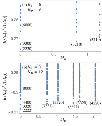
Figure 1: Eigenenergies per electron on the torus as a function of momentum at filling factor $\nu=2/3$ for $N_{e}=2N_{\Phi}/3=6$ (a), and $N_{e}=2N_{\Phi}/3=8$ (b). The $(N_{1}N_{2}N_{3}N_{4})$ labels specify the highest weight of selected multiplets. These results are for torus aspect ratio equal to one. We find that the low-energy spectrum is robust against aspect ratio variations.

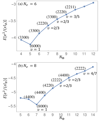
Figure 2: Ground state energy as a function of $N_{\Phi}$ on the sphere for $N_{e}=6$ (a), and $N_{e}=8$ (b). The filling factors assignments are based on comparisons between torus and sphere spectra.

By applying periodic boundary conditions on a torus, magnetic translational symmetry can be used to classify many-body states Haldane . Fig. 1 shows energy as a function of momentum at filling factor $\nu=2/3$. In Fig. 1(a), $N_{\Phi}$ and $N_{e}$ are respectively 9 and 6, and the ground state is a SU(3) singlet that has zero momentum, implying that it is a translationally invariant quantum fluid state. The first excited state at zero momentum is the well-known SU(2) singlet Zhang84 ; Xie89 described in the introduction. The third excited state at zero momentum is the single-component particle-hole conjugate state of the $\nu=1/3$ Laughlin state.

In Fig. 1(b), $N_{\Phi}$ and $N_{e}$ are increased to 12 and 8 respectively, and the ground state is a SU(4) singlet at zero momentum. The first and second excited states at zero momentum, labeled by $(3320)$ and $(4400)$, are very close in energy. The particle-hole conjugate of the $\nu=1/3$ Laughlin state has a higher energy and is buried deep in the continuum.

To determine the shift $\mathcal{S}$ of the $\nu=2/3$ singlets on the sphere, we vary $N_{\Phi}$ while keeping $N_{e}$ fixed. Fig. 2 shows the ground state energy on the sphere as a function of $N_{\Phi}$ at $N_{e}=6$ (Fig. 2(a)) and $N_{e}=8$ (Fig. 2(b)). For $N_{e}=6$ (Fig. 2(a)), the ground state at $N_{\Phi}=8$ is a SU(2) singlet, which is the composite-fermion singlet with $\nu=2/3$ and $\mathcal{S}=1$. At $N_{\Phi}=7$, the ground state is our new SU(3) singlet at $\nu=2/3$ with $\mathcal{S}=2$. Note that a SU(3) singlet also appears at $N_{\Phi}=9$, which we identify as a composite-fermion SU(3) singlet with $\nu=3/5$ and $\mathcal{S}=1$. The analysis of Fig. 2(b) is similar. We identify the SU(4) singlet at $N_{e}=8$ and $N_{\Phi}=10$ to $\nu=2/3$ with shift $\mathcal{S}=2$.

In Table 1, we compare the Coulomb energies between the SU(3) and SU(4) singlets and the SU(2)singlet at $\nu=2/3$ Ne_12 . In graphene Zeeman energy favors the SU(2) singlet which can have full spin polarization. Ideally, one would observe a transition from the new singlet states discovered here as the magnetic field is increased. The absence of an apparent transition in current experiments Yacoby12 might be explained by screening Misha ; Sodemann2014 and Landau level mixing effects Nayak2013 ; Sodemann2013 which tend to weaken effective interaction strengths, reducing the critical fields to values where it is challenging to observe the fractional quantum Hall effect.

The largest system size we have attempted is on a torus with $N_{e}=2N_{\Phi}/3=10$. For this number of electrons it is impossible to construct exact SU(3) or SU(4) singlets. We restricted the numerical calculation to 3-fold degenerate LLs, and found that a multiplet labeled by $(4420)$ has a lower energy than the SU(2) singlet. This adds to evidence that the $\nu=2/3$ SU(2) singlet predicted by composite fermion theory is not the ground state in LLs with more than two components. We hope that future studies will be able to extend our study to larger system sizes.

Table 1: Energy difference per electron between SU(3) or SU(4) and SU(2) singlet states on a torus at $\nu=2/3$. $\Delta E_{C}$ is the energy difference for pure Coulomb interaction. $\Delta E_{Z}$ is the Zeeman coupling energy difference between states in graphene with a $g-$factor of 2. $\mu_{B}$ is the Bohr magneton. For comparison, $[\mu_{B}B]/[e^{2}/(\epsilon l_{B})]=10^{-3}\epsilon\sqrt{B[T]}$. The critical field $B_{c}$ is obtained by setting $\Delta E_{C}+\Delta E_{Z}$ to 0.

	$\Delta E_{C}/N_{e}[e^{2}/(\epsilon l_{B})]$	$\Delta E_{Z}/N_{e}[\mu_{B}B]$	$B_{c}[T]$
(2220),(3300)	$-2.7203\times 10^{-3}$	2/3	$16.65/\epsilon^{2}$
(2222),(4400)	$-2.3015\times 10^{-3}$	1	$5.30/\epsilon^{2}$

Pair Correlation functions:— We now discuss the spatial correlation functions that describe the probability of finding two electrons at certain distance from each other. We have found that our new SU(3) and SU(4) singlets have similar short-distance correlations to the conventional SU(2) singlet and single component state at $\nu=2/3$, and the long-distance correlations are different. The flavor-dependent spatial correlation function $g_{\alpha\beta}(\vec{r})$ is defined by

$$g_{\alpha\beta}(\vec{r})=\frac{A}{N_{\alpha}N_{\beta}}\sum_{i\neq j}\delta(\vec{r}_{i}-\vec{r}_{j}-\vec{r})\big{(}|\chi_{\alpha}\rangle\langle\chi_{\alpha}|\big{)}_{i}\big{(}|\chi_{\beta}\rangle\langle\chi_{\beta}|\big{)}_{j},$$ (2)

where $A$ is the area of the 2D system, and $N_{\alpha}$ is the number of electrons in flavor state $|\chi_{\alpha}\rangle$.

Figs. 3(a) and (b) plot $g_{\alpha\beta}(\vec{r})$ of $\nu=2/3$ states along the diagonal line of the torus, i.e. along $r_{x}=r_{y}$. As required by the Pauli exclusion principle, $g_{11}(r)$ vanishes as $r\rightarrow 0$. It turns out that $g_{12}(r)$ is very small, but not exactly zero, at $r=0$ for the singlets. In graphene, SU(4) symmetry is weakly broken by short-range interactions that arise from lattice-scale Coulomb interactions and electron-phonon interactions. The short-range interactions are typically modeled by a $\delta-$function potential Kharitonov_MLG . Since the probability for two electrons to spatially overlap is small in these $\nu=2/3$ singlets, the short-range interactions should have an negligible effect on these states Halperin13 ; Inti14 ; Wu14 .

At small electron separation, $g_{11}(r)$ is similar in all singlet states, and likewise $g_{12}(r)$, with $g_{12}(r)$ smaller than $g_{11}(r)$ as shown in Fig. 3(a) and (b). We note that the four-component Halperin wavefunction with $m_{s}=3$ and $m_{d}=1$ has the opposite behavior, i.e. $g_{12}(r)>g_{11}(r)$ for small $r$. This is another distinct feature between the Halperin wavefunction and the exact SU(4) singlet, besides the difference in the shift.

The similarities between the pair correlation functions of different singlet states at small $r$ do not extend to larger distances. For the SU(2) singlet, $g_{11}(\vec{r})$ reaches a maximum at the maximum particle separation, while $g_{12}(\vec{r})$ reaches its maximum closer. The opposite behavior applies for SU(3) and SU(4) singlets at the system sizes we are able to study, as illustrated in Fig. 3.

To get a deeper understanding of the small $r$ behavior of $g_{\alpha\beta}(\vec{r})$, we consider the relative-angular-momentum (RAM) correlation function $\mathcal{L}_{\alpha\beta}(m)$:

$$\mathcal{L}_{\alpha\beta}(m)=\frac{2N_{\Phi}}{N_{\alpha}N_{\beta}}\sum_{i\neq j}P_{m}^{i,j}\big{(}|\chi_{\alpha}\rangle\langle\chi_{\alpha}|\big{)}_{i}\big{(}|\chi_{\beta}\rangle\langle\chi_{\beta}|\big{)}_{j},$$ (3)

where $P_{m}^{i,j}$Jain projects electrons $i$ and $j$ onto a state of RAM $m$. $\mathcal{L}_{\alpha\beta}(m)$ contains the same information as $g_{\alpha\beta}(\vec{r})$ and can be more physically revealing:

$$g_{\alpha\beta}(\vec{r})=\pi l_{B}^{2}\sum_{m}|\eta_{m}(\vec{r})|^{2}\mathcal{L}_{\alpha\beta}(m),$$ (4)

where $\eta_{m}$ is the wave-function for a state of a RAM $m$ Jain . At small electron separation $r$, $g_{\alpha\beta}(\vec{r})$ is mainly determined by $\mathcal{L}_{\alpha\beta}(m)$ with small $m$,

$$g_{\alpha\beta}(\vec{r})\approx \frac{1}{4}\mathcal{L}_{\alpha\beta}(0)+\frac{1}{16}[\mathcal{L}_{\alpha\beta}(1)-\mathcal{L}_{\alpha\beta}(0)](r/l_{B})^{2}$$ (5)

$$\approx \frac{1}{16}\mathcal{L}_{\alpha\beta}(1)(r/l_{B})^{2}.$$

The approximation in the second line of Eq. (5) follows from the fact that $\mathcal{L}_{\alpha\beta}(0)=4g_{\alpha\beta}(0)$ is always extremely small for states we consider. Values of $\mathcal{L}_{\alpha\beta}(1)$ are displayed in Fig. 3(c). Like the pair correlation functions, $\mathcal{L}_{\alpha\beta}(1)$ has similar values in all singlet states for both $\alpha=\beta$ and $\alpha\neq\beta$. As proved in the Supplemental Material, $\langle\mathcal{L}_{11}(1)\rangle_{s}=2\langle\mathcal{L}_{12}(1)\rangle_{s}$ in any singlet state. This property explains why $g_{12}(r)$ is smaller than $g_{11}(r)$ at small $r$.

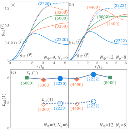
Figure 3: (Color online) (a) and (b) Correlation function $g_{\alpha\beta}(\vec{r})$ for the single-component state and the multi-component singlets at $\nu=2/3$. The direction of $\vec{r}$ is along the diagonal line of the torus. Solid and dashed lines distinguishes intra-flavor and inter-flavor correlation functions. (c) RAM correlation function $\mathcal{L}_{\alpha\beta}(m)$ with $m=1$. Filled and empty symbols designate intra-flavor and inter-flavor correlation functions respectively. Note that for any singlet, $\langle\mathcal{L}_{11}(1)\rangle_{s}=2\langle\mathcal{L}_{12}(1)\rangle_{s}$.

The energy per electron of a SU($n$) singlet can be decomposed into contributions from interactions in different angular momenta channel:

$$\langle H/N_{e}\rangle_{s}=\sum_{m}V_{m}[\varepsilon_{m}(n)-(N_{e}-1)/N_{\Phi}],$$ (6)

$$\varepsilon_{m}(n)=\frac{\nu}{4}\big{[}\langle\mathcal{L}_{12}(m)\rangle_{s}+\frac{1}{n}\langle\mathcal{L}_{11}(m)-\mathcal{L}_{12}(m)\rangle_{s}\big{]},$$

where $V_{m}$ is the $m$th Haldane pseudopotential of the Coulomb interactionJain , and the term $(N_{e}-1)/N_{\Phi}$ takes into account the contribution from the neutralizing background. For the $\nu=2/3$ SU($n$) singlets described above, $\varepsilon_{0}(n)$ is approximately zero, while $\varepsilon_{1}(n)$ decreases as $n$ increases from 2 to 3 or 4. This analysis sheds light on why SU(3) and SU(4) singlets have lower energy than the SU(2) singlet at $\nu=2/3$.

Summary:— By diagonalizing the Coulomb interaction Hamiltonian for electrons in multicomponent $n=0$ Landau levels, we have discovered translationally invariant SU(3) and SU(4) singlet ground states at filling factor $\nu=2/3$. We have found these states in systems containing $6$ and $8$ electrons respectively, on both sphere and torus geometries. Both states on the sphere have shift $\mathcal{S}=2$. The pair correlation function of these states is similar to that of composite fermion SU(2) singlet state at short electron separation, and becomes different at large distances.

Our findings are striking because the states we have discovered do not fit into either the composite fermion or the multicomponent Halperin state patterns. These singlets are candidates to join the handful of important states that do not fit the simple composite fermion paradigm, such as the Pfaffian state MR1991 and Read-Rezayi states Read-Rezayi . It is remarkable that this novel physics occurs in the lowest Landau level where past experience has suggested that composite fermions best describe Coulomb interaction incompressible states.

Acknowledgments:—IS is thankful to Xiao-Gang Wen for illuminating discussions. Work at Austin was supported by the DOE Division of Materials Sciences and Engineering under Grant DE-FG03-02ER45958, and by the Welch foundation under Grant TBF1473. IS is supported by a Pappalardo Fellowship. We thank the Texas Advanced Computing Center (TACC) and IDRIS-CNRS Project 100383 for providing computer time allocations.

Supplemental Material

I Proof of $\langle\mathcal{L}_{11}(m)\rangle_{s}=2\langle\mathcal{L}_{12}(m)\rangle_{s}$ for odd $m$

The second quantized form of the RAM correlation function $\mathcal{L}_{\alpha\beta}(m)$ is

$$\mathcal{L}_{\alpha\beta}(m)=\frac{2N_{\Phi}}{N_{\alpha}N_{\beta}}\sum\mathcal{M}_{p_{1}p_{2}p_{3}p_{4}}^{(m)}c_{p_{1}\alpha}^{\dagger}c_{p_{2}\beta}^{\dagger}c_{p_{3}\beta}c_{p_{4}\alpha},$$ (7)

where $c^{\dagger}_{p\alpha}$ ($c_{p\alpha}$) is an electron creation (annihilation) operator with $p$ denoting the orbital index. The matrix element $\mathcal{M}_{p_{1}p_{2}p_{3}p_{4}}^{(m)}$ is

$$\mathcal{M}_{p_{1}p_{2}p_{3}p_{4}}^{(m)}= \int d^{2}\vec{r}_{1}\int d^{2}\vec{r}_{2}\phi_{p_{1}}^{*}(\vec{r}_{1})\phi_{p_{2}}^{*}(\vec{r}_{2})$$ (8)

$$\times P_{m}^{1,2}\phi_{p_{3}}(\vec{r}_{2})\phi_{p_{4}}(\vec{r}_{1}),$$

where $\phi_{p}(\vec{r})$ is the single particle wavefunction for orbital $p$.

We can define a correlation function $\Gamma_{\alpha\beta}(m)$ that is conjugate to $\mathcal{L}_{\alpha\beta}(m)$,

$$\Gamma_{\alpha\beta}(m)=\frac{2N_{\Phi}}{N_{\alpha}N_{\beta}}\sum\mathcal{M}_{p_{1}p_{2}p_{3}p_{4}}^{(m)}c_{p_{1}\alpha}^{\dagger}c_{p_{2}\beta}^{\dagger}c_{p_{3}\alpha}c_{p_{4}\beta}.$$ (9)

The RAM projector has the property,

$$P_{m}^{1,2}\phi_{p_{3}}(\vec{r}_{2})\phi_{p_{4}}(\vec{r}_{1})=(-1)^{m}P_{m}^{1,2}\phi_{p_{4}}(\vec{r}_{2})\phi_{p_{3}}(\vec{r}_{1}),$$ (10)

which leads to:

$$\Gamma_{\alpha\beta}(m)=(-1)^{m+1}\mathcal{L}_{\alpha\beta}(m).$$ (11)

An immediate consequence is that $\mathcal{L}_{\alpha\alpha}(m)=0$ for even $m$, which is expected from Pauli exclusion principle.

A SU($n$) singlet state $|\Psi_{s}\rangle$ is invariant under a unitary transformation,

$$c_{p\alpha}\mapsto U_{\alpha\gamma}c_{p\gamma},c_{p\alpha}^{\dagger}\mapsto c_{p\gamma}^{\dagger}U_{\gamma\alpha}^{\dagger},$$ (12)

where $U$ is a $n\times n$ unitary matrix ($n\geq 2$) that is independent of the orbital index $p$. By making use of this invariance and noting that particle number in each flavor is a good quantum number, we arrive at the following constraints:

$$\langle\mathcal{L}_{\alpha\beta}(m)\rangle_{s} =\sum_{\gamma,\lambda}|U_{\alpha\gamma}|^{2}|U_{\beta\lambda}|^{2}\langle\mathcal{L}_{\gamma\lambda}(m)\rangle_{s}$$ (13)

$$+\sum_{\gamma\neq\lambda}U_{\gamma\alpha}^{\dagger}U_{\lambda\beta}^{\dagger}U_{\beta\gamma}U_{\alpha\lambda}\langle\Gamma_{\gamma\lambda}(m)\rangle_{s},$$

$$\langle\Gamma_{\alpha\beta}(m)\rangle_{s} =\sum_{\gamma,\lambda}|U_{\alpha\gamma}|^{2}|U_{\beta\lambda}|^{2}\langle\Gamma_{\gamma\lambda}(m)\rangle_{s}$$

$$+\sum_{\gamma\neq\lambda}U_{\gamma\alpha}^{\dagger}U_{\lambda\beta}^{\dagger}U_{\beta\gamma}U_{\alpha\lambda}\langle\mathcal{L}_{\gamma\lambda}(m)\rangle_{s},$$

where $\langle...\rangle_{s}$ denotes the expectation value with respect to the singlet state $|\Psi_{s}\rangle$. The two constraints in Eq. (13) are imposed by an arbitrary unitary matrix $U$, and give rise to an identity,

$$\langle\mathcal{L}_{11}(m)\rangle_{s}=\langle\mathcal{L}_{12}(m)\rangle_{s}+\langle\Gamma_{12}(m)\rangle_{s}.$$ (14)

By combining Eq. (11) and (14), we can conclude that for odd $m$, $\langle\mathcal{L}_{11}(m)\rangle_{s}=2\langle\mathcal{L}_{12}(m)\rangle_{s}$.

II $\mathcal{L}(m)$ for particle-hole conjugates of single component Laughlin states

Consider the spinless Laughlin state at filling $\nu=1/m$, $\phi_{1/m}$, and its particle-hole conjugate $\phi_{(m-1)/m}$ at filling $\nu=(m-1)/m$, where $m$ is an odd integer. The expectation value of $\mathcal{L}(m^{\prime})$ evaluated in $\phi_{(m-1)/m}$ can be shown to be related to that evaluated in $\phi_{1/m}$ as follows:

$$\langle\phi_{(m-1)/m}|\mathcal{L}(m^{\prime})|\phi_{(m-1)/m}\rangle=\frac{m^{2}}{(m-1)^{2}}\left(1-\frac{2}{m}\right)\langle\phi_{1}|\mathcal{L}(m^{\prime})|\phi_{1}\rangle+\frac{1}{(m-1)^{2}}\langle\phi_{1/m}|\mathcal{L}(m^{\prime})|\phi_{1/m}\rangle$$ (15)

The expression is obtained using $\langle\phi_{1/m}|c_{p_{1}}^{\dagger}c_{p_{2}}|\phi_{1/m}\rangle=\delta_{p_{1},p_{2}}/m$.

III Trial wavefunctions

One strategy to construct trial SU($n$) singlets at $\nu=2/3$ is to start from a SU($n$) singlet state $\psi_{n}$ at filling $\nu=n$. $\psi_{n}$ is a Slater determinant state in which $n-$fold degenerate lowest LLs are fully occupied. In analogy with the flux attachment procedure, we can multiply $\psi_{n}$ by appropriate Jastrow-type factors. We note that the following SU(3) and SU(4) singlet wavefunctions $\Psi_{3}$ and $\Psi_{4}$ have Fermi statistics, filling factor $\nu=2/3$ and shift $\mathcal{S}=2$:

$$\Psi_{3}(\nu=2/3,\mathcal{S}=2) =\Big{[}\text{Pf}\big{(}\frac{1}{z_{i}-z_{j}}\big{)}\phi^{L}_{6/7}\Big{]}\psi_{3},$$ (16)

$$\Psi_{4}(\nu=2/3,\mathcal{S}=2) =\Big{[}\text{Pf}\big{(}\frac{1}{z_{i}-z_{j}}\big{)}\phi^{L}_{4/5}\Big{]}\psi_{4},$$

Here $z_{i}$ denotes the complex coordinate of the $i$th electron. Pf indicates a Pfaffian factor, like the one appearing in the Moore-Read wavefunction MR1991 . $\phi^{L}_{6/7}$ and $\phi^{L}_{4/5}$ are wavefunctions for the single-component particle-hole conjugates of the $\nu=1/7$ and $\nu=1/5$ Laughlin states respectively. The Jastrow-type factors, that appear in square brackets are chosen to be completely symmetric functions of all the particle coordinates. Because $\psi_{n}$ have Fermi statistics and shift $\mathcal{S}=1$, and the conjugate Laughlin states have Fermi statistics and shift $\mathcal{S}=0$, the Pfaffian factor is required both to restore Fermi statistics and to increase the shift by 1.

In counting the filling factor and shift, we have used the rule that shifts and inverse of filling factors of holomorphic functions are additive under wavefunction multiplication:

$$F(\nu,\mathcal{S})=F_{1}(\nu_{1},\mathcal{S}_{1})F_{2}(\nu_{2},\mathcal{S}_{2}),$$ (17)

$$\nu^{-1}=\nu_{1}^{-1}+\nu_{2}^{-1},\quad\mathcal{S}=\mathcal{S}_{1}+\mathcal{S}_{2},$$

where $F(\nu,\mathcal{S})$ is a wavefunction with filling factor $\nu$ and shift $\mathcal{S}$.

Since $(z_{i}-z_{j})$ is a factor of $\phi^{L}_{6/7}$ and $\phi^{L}_{4/5}$ due to the antisymmetrization property, the Pfaffian factor does not lead to divergences in the trial wavefunctions. However, from the previous section one can conclude that the particle-hole conjugate of any single component Laughlin state has a finite probability of being in RAM with $m^{\prime}=1$, and, hence, that these Jastrow factors do not vanish in the limit $(z_{i}-z_{j})\to 0$. This implies that the full wavefunctions, $\Psi_{3}$ and $\Psi_{4}$, do not vanish when pairs of particles of different flavors approach each other. This appears to be in conflict with the qualitative behavior displayed by the pair correlations of the states found in exact diagonalization, depicted in Fig. 3 of the main text.

IV $\nu=p/3$ states in 4-fold degenerate Landau levels

The particle-hole symmetry in 4-fold degenerate LLs provides a one-to-one mapping between eigenstates at filling factor $\nu$ and those at $4-\nu$. Therefore, we can focus on $\nu\leq 2$ states. In the main text, we presented a detailed analysis of $\nu=2/3$ states. Here, we will discuss $\nu=p/3$ states with $p$=1, 4 and 5 based on exact diagonalization (ED) study on torus.

At $\nu=1/3$, we performed an ED study with $N_{\Phi}$ up to 15 and the ground state multiplet is represented by a single-component state, for which the $1/3$ Laughlin state is a good approximation.

Before discussing $\nu=4/3$ and 5/3 states, we first recall two useful mappings studied in Ref. Inti14, , which generates states at $\nu^{\prime}\in[1,2]$ from seed states at $\nu\in[0,1]$. Mapping-I is the particle-hole conjugation restricted to two-components,

$$(N_{1}N_{2}00),\nu\mapsto((N_{\Phi}-N_{1})(N_{\Phi}-N_{2})00),2-\nu;$$ (18)

$$E_{2-\nu}=E_{\nu}+2(1-\nu)E_{1},$$

where $E_{\nu}$ and $E_{2-\nu}$ are the Coulomb energies per flux quantum and $E_{1}=-\sqrt{\pi/8}e^{2}/(\epsilon l_{B})$. Mapping-II attaches a fully occupied LL to a seed wavefunction with three components or less,

$$(N_{1}N_{2}N_{3}0),\nu\mapsto(N_{\Phi}N_{1}N_{2}N_{3}),1+\nu;$$ (19)

$$E_{1+\nu}=E_{\nu}+E_{1}.$$

At $\nu=4/3$, ED on torus with $N_{\Phi}$ of 6 and 9 shows that the ground state multiplet is represented by a SU(2) singlet $(2N_{\Phi}/3,2N_{\Phi}/3,0,0)$, which can be generated from the SU(2) singlet at $\nu=2/3$ by Mapping-I.

At $\nu=5/3$, the ground state multiplet with $N_{\Phi}=9$ is represented by (9222), which is connected to (2220) state at $\nu=2/3$ through Mapping-II. We are not able to perform ED for every sector in the Hilbert space when $N_{\Phi}$ is increased to 12 or 15. However, we can still make the following two predictions based on ED results at $\nu=2/3$ and Mapping-II. One prediction is that (12, 3, 3, 2) has very similar energy as (12, 4, 4, 0) for $N_{\Phi}=12$. Another one is that (15, 4, 4, 2) has a lower energy compared to (15, 5, 5, 0) for $N_{\Phi}=15$. These finite-size results tend to suggest that $(N_{\Phi},N_{\Phi}/3,N_{\Phi}/3,0)$ is not the ground state at $\nu=5/3$ in SU(4) LLs.

References

- (1) B. I. Halperin, Helv. Phys. Acta 56, 75 (1983).
- (2) R. B. Laughlin, Phys. Rev. Lett. 50, 1395 (1983).
- (3) S. L. Sondhi, A. Karlhede, S. A. Kivelson, and E. H. Rezayi, Phys. Rev. B 47, 16419 (1993).
- (4) J. Eisenstein and A.H. MacDonald, Nature 432, 691 (2004).
- (5) J. Eisenstein, Ann. Rev. of Cond. Matt. Phys. 5, 159 (2014).
- (6) Y. W. Suen, L. W. Engel, M. B. Santos, M. Shayegan, and D. C. Tsui, Phys. Rev. Lett. 68, 1379 (1992).
- (7) Y. Liu, S. Hasdemir, D. Kamburov, A. L. Graninger, M. Shayegan, L. N. Pfeiffer, K. W. West, K. W. Baldwin, and R. Winkler, Phys. Rev. B 89, 165313 (2014).
- (8) Y. Liu, S. Hasdemir, J. Shabani, M. Shayegan, L. N. Pfeiffer, K. W. West, and K. W. Baldwin, arXiv:1501.06958.
- (9) K. S. Novoselov, A. K. Geim, S. V. Morozov, D. Jiang, M. I. Katsnelson, I. V. Grigorieva, S. V. Dubonos, A. A. Firsov, Nature 438, 197 (2005).
- (10) K. S. Novoselov, E. McCann, S. V. Morozov, V. I. Fal’ko, M. I. Katsnelson, U. Zeitler, D. Jiang, F. Schedin, and A. K. Geim, Nature Physics 2, 177-180 (2006).
- (11) T. Taychatanapat, K. Watanabe, T. Taniguchi, and P. Jarillo-Herrero, Nature Physics 7, 621-625 (2011).
- (12) A. L. Grushina, D.-K. Ki, M. Koshino, A. A. L. Nicolet, C. Faugeras, E. McCann, M. Potemski, and A. F. Morpurgo, Nature Communications 6, 6419 (2015).
- (13) N. C. Bishop, M. Padmanabhan, K. Vakili, Y. P. Shkolnikov, E. P. De Poortere, and M. Shayegan, Phys. Rev. Lett. 98, 266404 (2007).
- (14) D. Maryenko, J. Falson, Y. Kozuka, A. Tsukazaki, M. Onoda, H. Aoki, and M. Kawasaki, Phys. Rev. Lett. 108, 186803 (2012).
- (15) D. Maryenko, J. Falson, Y. Kozuka, A. Tsukazaki, and M. Kawasaki, Phys. Rev. B 90, 245303 (2014).
- (16) R. T. Weitz, M. T. Allen, B. E. Feldman, J. Martin, and A. Yacoby, Science 330, 812 (2010).
- (17) A. F. Young, J. D. Sanchez-Yamagishi, B. Hunt, S. H. Choi, K. Watanabe, T. Taniguchi, R. C. Ashoori, and P. Jarillo-Herrero, Nature 505, 528-532 (2014).
- (18) M. Kharitonov, Phys. Rev. B 85, 155439 (2012).
- (19) D. A. Abanin, B. E. Feldman, A. Yacoby, and B. I. Halperin, Phys. Rev. B 88, 115407 (2013).
- (20) I. Sodemann and A. H. MacDonald, Phys. Rev. Lett. 112, 126804 (2014).
- (21) F. Wu, I. Sodemann, Y. Araki, A. H. MacDonald, and Th. Jolicoeur, Phys. Rev. B 90, 235432 (2014).
- (22) K. Nomura and A. H. MacDonald, Phys. Rev. Lett. 96, 256602 (2006).
- (23) A. F. Young, C. R. Dean, L. Wang, H. Ren, P. Cadden-Zimansky, K. Watanabe, T. Taniguchi, J. Hone, K. L. Shepard, and P. Kim, Nature Physics 8, 550-556 (2012).
- (24) J. Lee and S. Sachdev, Phys. Rev. B 90, 195427 (2014); Phys. Rev. Lett. 114, 226801 (2015).
- (25) C. R. Dean, A. F. Young, P. Cadden-Zimansky, L. Wang, H. Ren, K. Watanabe, T. Taniguchi, P. Kim, J. Hone, and K. L. Shepard, Nature Physics 7, 693-696 (2011).
- (26) B. E. Feldman, B. Krauss, J. H. Smet, and A. Yacoby, Science 337, 1196 (2012).
- (27) J. K. Jain, Phys. Rev. Lett. 63, 199 (1989).
- (28) J. K. Jain, Composite Fermions (Cambridge University Press, Cambridge, England, 2007).
- (29) C. Tőke and J. K. Jain, Phys. Rev. B 75, 245440 (2007).
- (30) C. Tőke and J. K. Jain, J. Phys.: Condens. Matter. 24, 235601 (2012).
- (31) A. C. Balram, C. Tőke, A. Wójs, and J. K. Jain, Phys. Rev. B 91, 045109 (2015).
- (32) X. Du, I. Skachko, F. Duerr, A. Luican, and E. Y. Andrei, Nature 462, 192-195 (2009).
- (33) K. I. Bolotin, F. Ghahari, M. D. Shulman, H. L. Stormer, and P. Kim, Nature 462, 196-199 (2009).
- (34) S. Geraedts, M. P. Zaletel, Z. Papić, and R. S. K. Mong, Phys. Rev. B 91, 205139 (2015).
- (35) M. R. Peterson, Y.-L. Wu, M. Cheng, M. Barkeshli, Z. Wang, and S. Das Sarma, Phys. Rev. B 92, 035103 (2015).
- (36) F. C. Zhang and T. Chakraborty, Phys. Rev. B 30, 7320(R) (1984).
- (37) X. C. Xie, Y. Guo, and F. C. Zhang, Phys. Rev. B 40, 3487(R) (1989).
- (38) M. O. Goerbig and N. Regnault, Phys. Rev. B 75, 241405(R) (2007).
- (39) Z. Papić, M. O. Goerbig, and N. Regnault, Phys. Rev. Lett. 105, 176802 (2010).
- (40) X. G. Wen and A. Zee, Phys. Rev. Lett. 69, 953 (1992).
- (41) X. G. Wen, Adv. in Phys. 44, 405 (1995).
- (42) N. Read and E. H. Rezayi, Phys. Rev. B 84, 085316 (2011).
- (43) S. C. Davenport, Ph. D. thesis, University of Oxford, 2013; S. C. Davenport and S. H. Simon, Phys. Rev. B 85, 245303 (2012).
- (44) X. G. Wu, G. Dev, and J. K. Jain, Phys. Rev. Lett. 71, 153 (1993).
- (45) H. Georgi, Lie Algebras In Particle Physics: From Isospin To Unified Theories (Westview Press, Boulder, Colorado, 1999), Chap. 8.
- (46) F. D. M. Haldane, Phys. Rev. Lett. 55, 2095 (1985).
- (47) A direct energy comparison between these two new singlets is not available because we could not reach the system size at which SU(3) and SU(4) singlets would compete.
- (48) I. Sodemann and M. M. Fogler, Phys. Rev. B 86, 115408 (2012).
- (49) I. Sodemann, Ph. D. thesis, University of Texas at Austin, 2014.
- (50) M. R. Peterson and C. Nayak, Phys. Rev. B 87, 245129 (2013); Phys. Rev. Lett. 113, 086401 (2014).
- (51) I. Sodemann and A. H. MacDonald, Phys. Rev. B 87, 245425 (2013).
- (52) G. Moore and N. Read, Nucl. Phys. B 360, 362 (1991).
- (53) N. Read and E. Rezayi, Phys. Rev. B 59, 8084 (1999).