Preliminary EoS for core-collapse supernova simulations with the QMC model

Abstract

In this work we present the preliminary results of a complete equation of state (EoS) for core-collapse supernova simulations. We treat uniform matter made of nucleons using the the quark-meson coupling (QMC) model. We show a table with a variety of thermodynamic quantities, which covers the proton fraction range $Y_{p}=0-0.65$ with the linear grid spacing $\Delta Y_{p}=0.01$ ($66$ points) and the density range $\rho_{B}=10^{14}-10^{16}$g.cm^-3 with the logarithmic grid spacing $\Delta$log${}_{10}(\rho_{B}/[$g.cm${}^{-3}])=0.1$ ($21$ points). This preliminary study is performed at zero temperature and our results are compared with the widely used EoS already available in the literature.

I Introduction

Although the theory related to supernova (SN) has made a remarkable progress in the past decade, there are many questions still to be answered. The catastrophic infall of the core of a massive star, reversed to trigger the powerful ejection of the stellar mantle and envelope in a supernova explosion, was identified as the crucial role in the synthesis of heavy elements. But when, why and how it happens is a fundamental problem of stellar astrophysics that remains to be explained. The implosion of stellar cores was also proposed as part of the scenario of the stellar death Janka (2012); Hoyle and Fowler (1960).

There are no doubts that supernovae explosions are an unique phenomenon in nature and an excellent laboratory to test extreme physics conditions. Unfortunately SN tends to happen once in a century per galaxy which makes the study of these great labs very difficult. Due to this observational difficulty, simulations of core-collapse supernova have played an important role in the study of supernovae explosions and their possible remnants. The equation of state of nuclear physics is a fundamental ingredient in the simulation of SN explosion. Simulations of core-collapse supernovae have to be fed with a wide range of thermodynamic conditions. Moreover, extremely high density and temperature may be achieved when black holes are formed by failed supernovae. To date, the temperature is believed to vary from zero to more than $100$ MeV, densities from $10^{5}$ to more than $10^{15}$ g.cm^-3 and the proton fraction up to about $0.6$. Fulfilling these conditions makes the construction of a complete EoS a very hard work, mainly at low densities, where a variety of sub-structures and light clusterization are possible. For these reasons, there are only few complete EoS available in the literature. The most commonly used EoS are those of Lattimer and Swesty Lattimer and Swesty (1991), Shen Shen et al. (1998, 2011) and Hempel Hempel et al. (2012).

The Lattimer Lattimer and Swesty (1991) EoS is based on a compressible liquid drop model with a Skyrme force for nucleon interactions. The Shen EoS from 1998 Shen et al. (1998) was the first equation of state for supernova simulations using a relativistic nuclear model. The upgrade to Shen’s work was published in 2011 Shen et al. (2011) with more points in the table and the inclusion of the $\Lambda$ hyperons. Both works developed by Shen were constructed with the relativistic mean field Walecka model Serot and Walecka (1986) using the TM1 Sugahara and Toki (1994) parameterization. Hempel’s EoS Hempel et al. (2012) is based on the TM1, TMA Toki et al. (1995) and FSUgold Todd-Rutel and Piekarewics (2005) parameterizations of the Walecka model and use the nuclear statistical equilibrium model of Hempel and Schaffner-Bielich Hempel and Schaffner-Bielich (2010), which includes excluded volume effects.

Model	M	$m_{q}$	$m_{\sigma}$	$m_{\omega}$	$m_{\rho}$	$g_{\rho}$	$g_{\omega}$	$g_{\sigma}$	$B_{N}^{1/4}$	NLT	DDP
	(MeV)	(MeV)	(MeV)	(MeV)	(MeV)				(MeV)
QMC	939.0	5.5	550	783	770	8.6510	8.9817	5.9810∗	210.85	no	no
NL3	939.0	–	508.194	782.501	763	8.9480	12.868	10.217	–	yes	no
GM1	939.0	–	550	783	770	8.1945	10.608	9.5684	–	yes	no
TM1	938.0	–	511.197	783	770	4.6321	12.613	10.028	–	yes	no
FSUgold	939.0	–	491.5	782.5	763	11.7673	14.301	10.592	–	yes	no
TMA†	938.9	–	519.151	781.95	768.1	3.800	12.842	10.055	–	yes	no
TW	939.0	–	550	783	763	7.32196∗∗	13.2901∗∗	10.728∗∗	–	no	yes

Table 1: Parameters used in the QMC model and different Walecka model parameterizations. In the first line we present the parameters used in the present work with the QMC model. The NL3, GM1 and TW parameterizations of the Walecka model are used here for a comparison of bulk matter properties. TM1 is the parameterization used in Shen’s work. The FSUgold and TMA were used in Hempel’s work. ${}^{*}g^{q}_{\sigma}$ is the quark-meson coupling in the QMC model. ^∗∗ values taken at saturation for the TW parameterization. TMA^†: the coupling parameters $g_{i}$ of the set TMA are chosen to be mass-number dependent such that $g_{i}=a_{i}+b_{i}/A^{0.4}$, with $a_{i}$ and $b_{i}$ being constants Toki et al. (1995); for infinite matter as in the stellar matter, one has an infinite nucleus, and then the limit A $\mapsto$ infinity is taken so that $g_{i}=a_{i}$. NLT= Nonlinear terms. DDP= Density dependent parameters.)

An interesting analysis of the different parameterizations of the relativistic-mean-field (RMF) models was made by Dutra et al Dutra et al. (2014), where the authors analyzed 263 different RMF models under several constrains related to the symmetric nuclear matter (SNM) and pure neutron matter (PNM). The TM1 parameterization used by Shen failed under six of this constraints, the TMA used by Hempel failed in five, and the FSUgold, also used by Hempel failed in one constraint. More details of this analysis in Dutra et al. (2014).

The works of Hempel, Lattimer and Shen were successful and very useful in many calculations in the last decade Sekiguchi et al. (2015); Nasu et al. (2015); Abdikamalov et al. (2014); Fryer and Heger (2000); Thompson and Pinto (2003); Pejcha and Thompson (2015), but there are some simulations of SN in which the supernova does not explode Buras et al. (2003). It is believed that these failures are due to some problems with the nuclear EoS.

In this work we present our preliminary results for the construction of an EoS grid for core-collapse supernova simulations, with the quark-meson coupling (QMC) model Guichon (1988).

In the QMC model, nuclear matter is described as a system of non-overlapping MIT bags Chodos et al. (1974) that interact through the exchange of scalar and vector meson fields. Many applications and extensions of the model have been made in the last years Fleck et al. (1990); Saito and Thomas (1994, 1995); Guichon et al. (1996); Panda et al. (2004). It is found that the EoS for infinite nuclear matter at zero temperature derived from the QMC model is softer than the one obtained with the Walecka model. This might be a problem if one wants to describe very massive compact objects Demorest et al. (2010); Antoniadis et al. (2013), but as far as SN simulations are concerned, it is worth testing it because apart from numerical accordance, one can interpret that starting from quark degrees of freedom is an advantage on the physical meaning underneath. Moreover, the effective nucleon mass obtained with the QMC model lies in the range 0.7-0.8 of the free nucleon mass, which agrees with the results derived from the non-relativistic analysis of scattering of neutrons from lead nuclei Johnson and Mahaux (1987) and is larger in comparison with the effective mass obtained with some of the different parameterizations of the Walecka models. A low effective mass at saturation can be a problem when hyperons are included in the calculation, as discussed in the next section.

All the few works for the purpose of the SN simulations that are based on relativistic models, use different parameterizations of the Walecka model, in which the nucleons interact between each other through the exchange of mesons. We believe that with the quarks degree of freedom present in the QMC model, a more fundamental physics lacking in the already used models, can be tested and possibly contribute for the SN simulations to explode.

Another possible use of this preliminary EoS obtained with the QMC model is the study of the cooling of compact stars, which serve as an important window on the properties of super-dense matter and neutron star structure, and is very sensitive to the nuclear equation of state Page et al. (2006); Negreiros et al. (2013); Fortin et al. (2010); de Carvalho et al. (2014).

This paper is structured as follows: in the second section we present a review of the quark-meson coupling model. In the third section we present our results for the EoS. The last section is reserved for the final remarks and conclusions.

II The quark-meson coupling model

In the QMC model, the nucleon in nuclear medium is assumed to be a static spherical MIT bag in which quarks interact with the scalar ($\sigma$) and vector ($\omega$, $\rho$) fields, and those are treated as classical fields in the mean field approximation (MFA) Guichon (1988). The quark field, $\psi_{q_{N}}$, inside the bag then satisfies the equation of motion:

$$\left[i\,\hbox to0.0pt{/\hss}\partial\right. - (m_{q}^{0}-g_{\sigma}^{q}\,)-g_{\omega}^{q}\,\omega\,\gamma^{0}$$ (1)

$$+ \left.\frac{1}{2}g^{q}_{\rho}\tau_{z}\rho_{03}\gamma^{0}\right]\,\psi_{q_{N}}(x)=0\ ,\quad q=u,d$$

where $m_{q}^{0}$ is the current quark mass, and $g_{\sigma}^{q}$, $g_{\omega}^{q}$ and $g_{\rho}^{q}$ denote the quark-meson coupling constants. The normalized ground state for a quark in the bag is given by

$$\psi_{q_{N}}({\bf r},t) = {\cal N}_{q_{N}}\exp\left(-i\epsilon_{q_{N}}t/R_{N}\right)$$ (4)

$$\times \left(\begin{array}[]{c}j_{0_{N}}\left(x_{q_{N}}r/R_{N}\right)\\ i\beta_{q_{N}}\vec{\sigma}\cdot\hat{r}j_{1_{N}}\left(x_{q_{N}}r/R_{N}\right)\end{array}\right)\frac{\chi_{q}}{\sqrt{4\pi}}~{},$$

where

$$\epsilon_{q_{N}}=\Omega_{q_{N}}+R_{N}\left(g_{\omega}^{q}\,\omega+\frac{1}{2}g^{q}_{\rho}\tau_{z}\rho_{03}\right),$$ (5)

and,

$$\beta_{q_{N}}=\sqrt{\frac{\Omega_{q_{N}}-R_{N}\,m_{q}^{*}}{\Omega_{q_{N}}\,+R_{N}\,m_{q}^{*}}}\ ,$$ (6)

with the normalization factor given by

$${\cal N}_{q_{N}}^{-2}=2R_{N}^{3}j_{0}^{2}(x_{q})\left[\Omega_{q}(\Omega_{q}-1)+R_{N}m_{q}^{*}/2\right]\Big{/}x_{q}^{2}~{},$$ (7)

where $\Omega_{q_{N}}\equiv\sqrt{x_{q_{N}}^{2}+(R_{N}\,m_{q}^{*})^{2}}$, $m_{q}^{*}=m_{q}^{0}-g_{\sigma}^{q}\,\sigma$, $R_{N}$ is the bag radius of nucleon $N$ and $\chi_{q}$ is the quark spinor. The bag eigenvalue for nucleon $N$, $x_{q_{N}}$, is determined by the boundary condition at the bag surface

$$j_{0_{N}}(x_{q_{N}})=\beta_{q_{N}}\,j_{1_{N}}(x_{q_{N}})\ .$$ (8)

The energy of a static bag describing nucleon $N$ consisting of three quarks in ground state is expressed as

$$E^{\rm bag}_{N}=\sum_{q}n_{q}\,\frac{\Omega_{q_{N}}}{R_{N}}-\frac{Z_{N}}{R_{N}}+\frac{4}{3}\,\pi\,R_{N}^{3}\,B_{N}\ ,$$ (9)

where $Z_{N}$ is a parameter which accounts for zero-point motion of nucleon $N$ and $B_{N}$ is the bag constant. The set of parameters used in the present work is determined by enforcing stability of the nucleon (here, the “bag”), much like in Santos and Providência (2009), so there is a single value for proton and neutron masses. The effective mass of a nucleon bag at rest is taken to be $M_{N}^{*}=E_{N}^{\rm bag}.$

The equilibrium condition for the bag is obtained by minimizing the effective mass, $M_{N}^{*}$ with respect to the bag radius

$$\frac{d\,M_{N}^{*}}{d\,R_{N}^{*}}=0,\,\,\;\;\;N=p,n,$$ (10)

By fixing the bag radius $R_{N}=0.6$ fm and the bare nucleon mass $M=939$ MeV the unknowns $Z_{N}=4.0050668$ and $B^{1/4}_{N}=210.85$MeV are then obtained. Furthermore, the desired values of $B/A\equiv\epsilon/\rho-M=-15.7$ MeV at saturation $n=n_{0}=0.15$ fm^-3, are achieved by setting $g_{\sigma}^{q}=5.9810$, $g_{\omega}=8.9817$, where $g_{\omega}=3g^{q}_{\omega}$ and $g_{\rho}=3g^{q}_{\rho}$. All the parameters used in this work are shown in Table 1.

The total energy density of the nuclear matter reads

$$\varepsilon=\frac{1}{2}m^{2}_{\sigma}\sigma+\frac{1}{2}m^{2}_{\omega}\omega^{2}_{0}+\frac{1}{2}m^{2}_{\rho}\rho^{2}_{03}$$

$$+\sum_{N}\frac{1}{\pi^{2}}\int^{k_{N}}_{0}k^{2}dk[k^{2}-M^{*2}_{N}]^{1/2},$$ (11)

and the pressure is,

$$p=-\frac{1}{2}m^{2}_{\sigma}\sigma+\frac{1}{2}m^{2}_{\omega}\omega^{2}_{0}+\frac{1}{2}m^{2}_{\rho}\rho^{2}_{03}$$

$$+\sum_{N}\frac{1}{\pi^{2}}\int^{k_{N}}_{0}k^{4}dk/[k^{2}-M^{*2}_{N}]^{1/2}.$$ (12)

The vector mean field $\omega_{0}$ and $\rho_{03}$ are determined through

$$\omega_{0}=\frac{g_{\omega}(n_{p}+n_{n})}{m^{2}_{\omega}},\;\rho_{03}=\frac{g_{\rho}(n_{p}-n_{n})}{m^{2}_{\rho}},$$ (13)

where

$$n_{B}=\sum_{N}\frac{2k_{N}^{3}}{3\pi^{2}},\quad N=p,n.$$ (14)

is the baryon density.

Finally, the mean field $\sigma$ is fixed by imposing that

$$\frac{\partial\varepsilon}{\partial\sigma}=0.$$ (15)

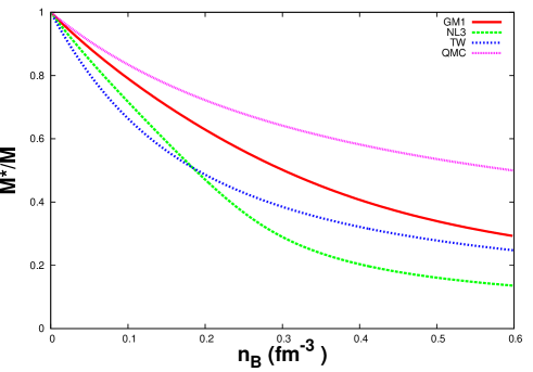
Figure 1: The effective mass of the QMC model and three Walecka parameterizations.

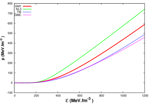
Figure 2: Equation of state of the QMC model and three Walecka model parameterizations.

Model	$B/A$	$n_{0}$	$M^{*}/M$	$\mathcal{E}_{sym}$	K
	(MeV)	(fm-3)		(MeV)	(MeV)
QMC	-15.7	0.150	0.77	34.5	295
NL3	-16.2	0.148	0.60	37.4	272
GM1	-16.3	0.153	0.70	32.5	300
TM1	-16.3	0.145	0.63	36.8	281
FSUgold	-16.3	0.148	0.62	32.6	230
TMA	-16.0	0.147	0.63	30.7	318
TW	-16.2	0.153	0.56	32.6	240

Table 2: Nuclear matter bulk properties obtained with the QMC model, two different parameterizations of Walecka model and one density dependent model we use in this paper, and the four parameterizations used in the works of Hempel and Shen. All quantities are taken at saturation.

It is always important to check the behavior of the models in the symmetric nuclear matter at saturation density and zero temperature, i.e., the bulk nuclear matter properties. A comprehensive work in this direction is Dutra et al. (2014), but the QMC model was not analyzed. Therefore, we compare the QMC model with two parameterization of the well known Walecka-type models, namely: GM1 Glendenning (Springer-Verlag, New York, 2000) and NL3 Lalazissis et al. (1997) and the density dependent parameter model TW Typel and Wolter (1999). In this work we have chosen GM1 for being a parameterization which gives a good value for the effective mass, NL3 because it is a very common standard parameterization and TW because it is a very good density dependent parameterization according to Dutra et al. (2014). In Dutra et al. (2014), it was found that GM1 failed under six constrains related to the symmetric nuclear matter (SNM) and pure neutron matter (PNM), NL3 failed under nine and TW did not satisfy only one constraint.

In Table 1 we can see the different parameters here analyzed and the ones used in the works of Shen Shen et al. (1998, 2011) and Hempel Hempel et al. (2012).

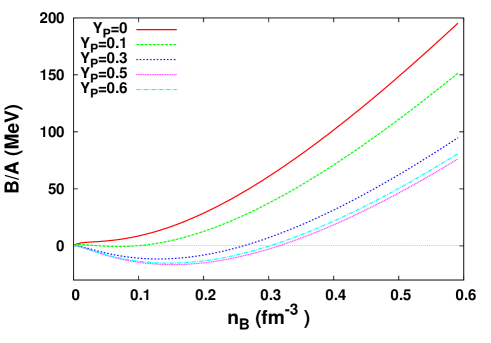
Figure 3: Binding energy of the nucleons as function of the baryon density with the proton fractions $Y_{p}=$0, 0.1, 0.3, 0.5 and 0.6.

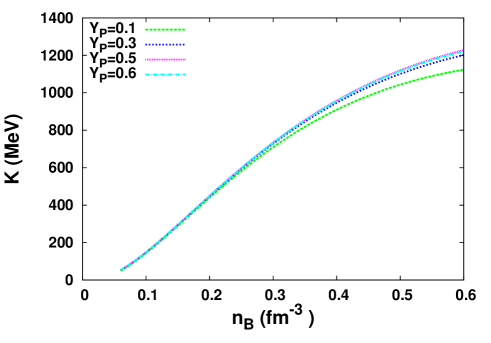
Figure 4: Compression modulus as function of the baryon density with the proton fractions $Y_{p}=$0.1, 0.3, 0.5 and 0.6.

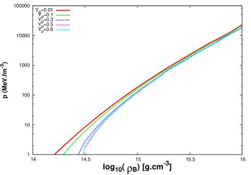
Figure 5: The relation between pressure and $\rho_{B}$ for the $Y_{p}=$0.01, 0.1, 0.3, 0.5 and 0.6 protons fractions.

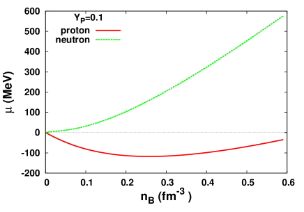
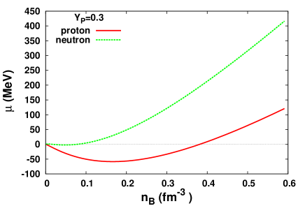
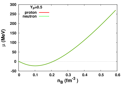
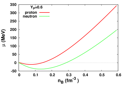
Figure 6: Some fixed values of proton fraction for chemical potentials as function of the baryonic density. The continuous line represents $\mu_{p}$ and the dashed line represents $\mu_{n}$.

In Table 2 we show the properties of nuclear matter at saturation density and zero temperature. The first column shows the binding energy per nucleon, the second shows the baryonic density of the nucleons at the saturation point, the third the effective mass relative to the free nucleon mass, the symmetry energy and the compression modulus of the nucleons.

In Fig. 1 we show the relation of the effective mass as function of the baryonic density where we can see that the effective mass for the QMC model has always a larger value than the other models, which is an important characteristic if hyperons are to be included. As can be seen in Santos and Menezes (2004) the effective mass of some of the Walecka-type models tend to zero at still low densities when all the baryons of the octet are included. For this reason, parameterizations with larger effective masses were proposed by Glendenning Glendenning (Springer-Verlag, New York, 2000) (GM1, GL, etc) with the specific purpose of applications to stellar matter. Note that in both, figure and table, we can see that $M^{*}/M=0.77$ at the saturation density, which agrees with the results derived from the non-relativistic analysis of scattering of neutrons from lead nuclei Johnson and Mahaux (1987), and that this result is larger in comparison with the effective mass from many of the Walecka-type models.

In Fig. 2 we show the pressure versus energy density relation for infinite nuclear matter at $T=0$, where we see that the curve for QMC is similar to the one for TW, and softer than the GM1 and NL3. As mentioned in the Introduction, this can be a deficiency for neutron star studies, but those effects on supernovae are still not analyzed.

III Results and discussions

In this work we construct an EoS table covering a wide range of proton fraction $Y_{p}$ and baryon density $n_{B}$. We show in the paper some results concerning the properties of matter with the QMC model and indicate the website from where the full table can be download.

We show in Fig. 3 the binding energy of homogeneous nuclear matter at zero temperature as a function of the baryon density for different proton fractions. For pure neutron matter and low proton fractions, there are no binding states, as expected. This result is in good agreement with Walecka Serot and Walecka (1986) and Shen Shen et al. (1998). In Fig. 4 we show the compression modulus versus the baryonic density, where the expression for $K$ is

$$K=9\;n_{B}^{2}\frac{d^{2}}{dn_{B}^{2}}\left(\frac{\varepsilon}{n_{B}}\right),$$ (16)

$n_{B}$ is the baryon number density and $\varepsilon$ the total energy density of the nucleons. Here we see that near the saturation density the compression modulus has the same value independent of the proton fraction and, as the density increases, the compression modulus is different for each $Y_{p}$.

In Fig. 5 the pressure $p$ as a function of $\rho_{B}$ is displayed. The baryon number density is related to the baryon mass density as $\rho_{B}=m_{u}n_{B}$ where $m_{u}=931.49432$ MeV is the atomic mass unit. We note that the pressure varies more with the $Y_{p}$ for low values of $p$ at lower densities, this result is also in good agreement with Shen’s work Shen et al. (1998).

In Fig. 6 we show the proton and neutron chemical potentials, $\mu_{p}$ and $\mu_{n}$, as function of the baryon density for the proton fractions $Y_{p}=0.1$, $0.3$, $0.5$ and $0.6$. In these curves we see that for $Y_{p}=0.1$ the chemical potential of the neutron is bigger than the one of the proton. As the proton fraction gets bigger, the curves approach each other, until they are the same in $Y_{p}=0.5$, and for $Y_{p}=0.6$ the chemical potential of the proton is bigger than the one of the neutron. This is an obvious result, but as the chemical potentials are very important quantities in the EoS tables, they are also presented graphically.

T	log10$(\rho_{B})$	$n_{B}$	YP	F	$E_{int}$	S	M*N	Xn	Xp	p	$\mu_{n}$	$\mu_{p}$
(MeV)	(g.cm-3)	(fm-3)		(MeV)	(MeV)	(kB)	(MeV)			(MeV fm-3)	(MeV)	(MeV)
0	14.0	0.0602	0	4.890	12.40	0	838.9	1	0	0.2371	23.43	-68.43
0	14.1	0.0758	0	6.090	13.60	0	816.9	1	0	0.5103	31.20	-82.21
0	14.2	0.0954	0	8.133	15.64	0	791.2	1	0	1.0890	42.68	-97.63
0	14.3	0.1201	0	11.56	19.07	0	761.5	1	0	2.2780	59.66	-114.3
0	14.4	0.1512	0	17.19	24.70	0	728.8	1	0	4.6550	84.64	-131.4

Table 3: EoS table at $T=0$. It covers the proton fraction range $Y_{p}=0-0.65$ with the linear grid spacing $\Delta Y_{p}=0.01$ (66 points), and the density range $\rho_{B}=10^{14}-10^{16}$ g cm^-3 with the logarithmic grid spacing $\Delta$log₁₀ $(\rho_{B}$ /[g cm${}^{-3}])=0.1$ (21 points). This table is available in the website . An exerpt of it is shown here for guidance.

Once bulk nuclear matter properties are shown to behave as expected and present some important differences as compared with the other works, we proceed toward building a preliminary EoS table with the QMC model, for homogeneous matter and zero temperature, which is available on the Web at

http://debora.fsc.ufsc.br/eos_qmc.t0.

In Table 3 we show the thermodynamic quantities described as in Shen et al. (1998, 2011)

1. Temperature: $T$[MeV].

2. Logarithm of baryon mass density: log₁₀($\rho_{B}$)[g.cm^-3].

3. Baryon number density: $n_{B}$ [fm^-3].
   

4. Proton fraction: Y_p.
   The proton fraction Y_p of uniform matter made of protons and neutrons, is defined by

   $$Y_{p}=\frac{n_{p}}{n_{n}+n_{p}}$$

   where $n_{p}$ and $n_{n}$ are the number density of protons and neutrons, respectively.

5. Free energy per baryon: $F$ [MeV].
   The free energy per baryon reads,

   $$f=\varepsilon-Ts.$$

   This work is for zero temperature only, hence $f=\varepsilon$. The free energy per baryon is defined relative to the nucleon mass as,

   $$F=\frac{\varepsilon}{n_{B}}-M=B/A.$$

6. Internal energy per baryon:$E_{int}$ [MeV].
   The internal energy per baryon is defined relative to the atomic mass unit $m_{u}=931.49432$ MeV as

   $$E_{int}=\frac{\varepsilon}{n_{B}}-m_{u}.$$

7. Entropy per baryon: $S$[$k_{B}$].
   The case we work here is for zero temperature, therefore $S=0$.

8. Effective nucleon mass: $M^{*}_{N}$ [MeV].
   The effective nucleon mass is obtained in the QMC model for uniform matter with the relation $M^{*}_{N}=E^{bag}_{N}$, where $N=p$, $n$, and the bag energy is obtained through the Eq. 9.

9. Free neutron fraction: $X_{n}$.

10. Free proton fraction: $X_{p}$.

11. Pressure: $p$ [MeV.fm^-3].
    The pressure is calculated from Eq. 12.

12. Chemical potential of the neutron: $\mu_{n}$ [MeV].
    For the zero temperature case, the chemical potential of the neutron relative to the free nucleon mass $M$ is calculate through the following equation

    $$\mu_{n}=[k_{n}^{2}+M^{*2}]^{1/2}+g_{\omega}\omega_{0}-\frac{g_{\rho}}{2}\rho_{03}-M.$$

13. Chemical potential of the proton: $\mu_{p}$ [MeV].
    For the zero temperature case, the chemical potential of the proton relative to the free nucleon mass $M$ is calculated through the following equation

    $$\mu_{p}=[k_{p}^{2}+M^{*2}]^{1/2}+g_{\omega}\omega_{0}+\frac{g_{\rho}}{2}\rho_{03}-M.$$

IV Conclusion and future works

In this work we have used the QMC model for the first time for the construction of a preliminary EoS that in the future can be useful for the studies involving cooling of neutron stars and supernova simulations. We believe that with the quarks degree of freedom present in the QMC model, the EoS can contribute with part of the physics that lack for SN simulations to explode.

The next step of the present work, already under development, is the computation of the EoS grid at finite temperature, which is essential for the supernova simulations.

Thereafter we will study the very low density regions, where nuclear matter is no longer uniform. This will be done with the pasta phase approach Maruyama et al. (2005); Providência et al. (2014). We believe that the use of the pasta phase for the description of the non-uniform part of matter that compose the EoS table in the SN simulations will certainly affect SN and cooling simulations.

References

- Janka (2012) H.-T. Janka, Ann. Rev. Nucl. Part. Sci. 62, 407 (2012).
- Hoyle and Fowler (1960) F. Hoyle and W. A. Fowler, Astrophys. J. 132, 565 (1960).
- Lattimer and Swesty (1991) J. M. Lattimer and F. D. Swesty, Nucl. Phys. A 535, 331 (1991).
- Shen et al. (1998) H. Shen et al., Nucl. Phys. A 637, 435 (1998).
- Shen et al. (2011) H. Shen et al., Astrophys. J. Suppl. 197, 20 (2011).
- Hempel et al. (2012) M. Hempel et al., Astrophys. J. 748, 70 (2012).
- Serot and Walecka (1986) B. D. Serot and J. D. Walecka, Adv. Nucl. Phys. 16, 1 (1986).
- Sugahara and Toki (1994) Y. Sugahara and H. Toki, Nucl. Phys. A 579, 557 (1994).
- Toki et al. (1995) H. Toki et al., Nucl. Phys. A 588, 357c (1995).
- Todd-Rutel and Piekarewics (2005) B. G. Todd-Rutel and J. Piekarewics, Phys. Rev. Lett. 95, 122501 (2005).
- Hempel and Schaffner-Bielich (2010) M. Hempel and J. Schaffner-Bielich, Nucl. Phys. A 837, 210 (2010).
- Dutra et al. (2014) M. Dutra et al., Phys. Rev. C 90, 055203 (2014).
- Sekiguchi et al. (2015) Y. Sekiguchi et al., Phys. Rev. D 91, 064059 (2015).
- Nasu et al. (2015) S. Nasu et al., Astrophys. J. 801, 78 (2015).
- Abdikamalov et al. (2014) E. Abdikamalov et al., Phys. Rev. D 90, 044001 (2014).
- Fryer and Heger (2000) C. L. Fryer and A. Heger, Astrophys. J. 541, 1033 (2000).
- Thompson and Pinto (2003) B. A. Thompson, T. A. and P. A. Pinto, Astrophys. J. Suppl. 592, 434 (2003).
- Pejcha and Thompson (2015) O. Pejcha and T. A. Thompson, Astrophys. J. 801, 90 (2015).
- Buras et al. (2003) R. Buras et al., Phys. Rev. Lett. 90, 241101 (2003).
- Guichon (1988) P. A. M. Guichon, Phys. Lett. B 200, 235 (1988).
- Chodos et al. (1974) A. Chodos et al., Phys. Rev. D 9, 3471 (1974).
- Fleck et al. (1990) S. Fleck et al., Nucl. Phys. A 510, 731 (1990).
- Saito and Thomas (1994) K. Saito and A. W. Thomas, Phys. Lett. B 327, 9 (1994).
- Saito and Thomas (1995) K. Saito and A. W. Thomas, Phys. Rev. C 52, 2789 (1995).
- Guichon et al. (1996) P. A. M. Guichon et al., Nucl. Phys. A 601, 349 (1996).
- Panda et al. (2004) P. K. Panda, D. P. Menezes, and C. Providência, Phys. Rev. C 69, 025207 (2004).
- Demorest et al. (2010) P. Demorest et al., Nature 467, 1081 (2010).
- Antoniadis et al. (2013) J. Antoniadis et al., Science 26, 6131 (2013).
- Johnson and Mahaux (1987) H. D. J. Johnson, C. H. and C. Mahaux, Phys. Rev. C 36, 2252 (1987).
- Page et al. (2006) D. Page, U. Geppert, and F. Weber, Nucl. Phys. A 777, 497 (2006).
- Negreiros et al. (2013) R. Negreiros, S. Schramm, and F. Weber, arXiv:1307.7692v1 astro-ph, 1 (2013).
- Fortin et al. (2010) M. Fortin et al., Phys. Rev. C 82, 065804 (2010).
- de Carvalho et al. (2014) S. M. de Carvalho et al., arXiv:1411.5316v1 astro-ph, 1 (2014).
- Santos and Providência (2009) A. M. Santos and C. Providência, Phys. Rev. C 79, 045805 (2009).
- Glendenning (Springer-Verlag, New York, 2000) N. K. Glendenning, Compact Stars (Springer-Verlag, New York, 2000).
- Lalazissis et al. (1997) G. A. Lalazissis, J. König, and P. Ring, Phys. Rev. C 55, 540 (1997).
- Typel and Wolter (1999) S. Typel and H. H. Wolter, Nucl. Phys. A 656, 331 (1999).
- Santos and Menezes (2004) A. M. S. Santos and D. P. Menezes, Phys. Rev. C 69, 045803 (2004).
- Maruyama et al. (2005) T. Maruyama et al., Phys. Rev. C 72, 015802 (2005).
- Providência et al. (2014) C. Providência et al., Eur. Phys. J. A 50, 44 (2014).