The Finslerian compact star model

Abstract

We construct a toy model for compact stars based on the Finslerian structure of spacetime. By assuming a particular mass function, we find an exact solution of the Finsler-Einstein field equations with an anisotropic matter distribution. The solutions are revealed to be physically interesting and pertinent for the explanation of compact stars.

I INTRODUCTION

Spherically symmetric spacetime related astrophysical problems have been always interesting to mathematician as well as physicists. This is because of the fact that phenomena such as black holes, wormholes and compact stars (starting from dwarf stars via neutron stars to quark/strange stars through the vigorous process of gravitational collapse) have been originated in the class of system with spherical symmetry.

After the monumental construction of Einstein’s general theory of relativity in the period 1907 to 1915 Pais1982 , numerous investigators have been started studying relativistic stellar models with various aspects of physical reality. The investigation of the exact solutions recounting static isotropic and anisotropic astrophysical objects has continuously fascinated scientists with growing interest and attraction. However, it has till now been observed that most of the exact interior solutions (both isotropic and anisotropic) of the gravitational field equations do not fulfill in general the required physical conditions of the stellar systems.

The existence of massive compact stellar system was first proposed by Baade and Zwicky in 1934 BZ1934 when they argued that supernova may yield a very small and dense star consisting primarily of neutrons. It eventually came in to reality by the discovery of pulsar, a highly magnetized and rotating neutron star, in 1967 by Bell and Hewish Longair1994 ; Ghosh2007 . There after, the theoretical investigation of compact stars became fundamental area of importance in astrophysics. However, for modeling a compact star emphasis has been given in general on the homogeneity of the spherically symmetric matter distribution and thus assumption was always valid for the perfect fluid obeying Tolman-Oppenheimer-Volkoff (TOV) equation.

It was Ruderman Ruderman1972 who first argued that the nuclear matter density ($\rho\sim 10^{15}$ gm/cc), which is expected at the core of the compact terrestrial object, becomes very much anisotropic. In such case of anisotropy the pressure inside the fluid sphere can specifically be decomposed into two parts: radial pressure and the transverse pressure, where they are orthogonal to each other. Therefore it is quite reasonable to consider pressure anisotropy in any compact stellar model. In this context it can be noted that Gokhroo and Mehra gokhroo1994 have shown that in case of anisotropic fluid the existence of repulsive force helps to construct compact objects.

Other than the above mentioned ultra density Ruderman1972 anisotropy may occur for different reasons in the compact stellar system. Kippenhahn and Weigert Kippenhahn1990 have argued that anisotropy could be introduced due to the existence of solid core or for the presence of type $3A$-superfluid. Some other reasonable causes for arising anisotropy are: different kind of phase transitions sokolov1980 , pion condensation  sawyer1972 , effects of slow rotation in a star Silva2014 etc. However, Bowers and Liang Bowers1974 indicated that anisotropy might have non-negligible effects on such parameters like equilibrium mass and surface redshift. In connection to pressure anisotropy inside a compact star several recent theoretical investigations are available in the literature Herrera2004 ; Varela2010 ; Rahaman2010a ; Rahaman ; Rahaman2012a ; Kalam2012 ; Hossein2012 ; Kalam2013 . However, there is an exhaustive review on the subject of anisotropic fluids by Herrera and Santos Herrera1997 which provides almost all references until 1997 and hence may be looked at for further information.

Several major characteristics of compact stars established by the present day observations have been tackled by Einstein’s general theory of relativity based on Riemannian geometry. Ever since the beginning of the general theory of relativity, there has also been considerable interest in Alternative theories of gravitation. One of the most stimulating alterations of general relativity is that proposed by Finsler Bao2000 .

The first self-consistent Finsler geometry model was studied by E. Cartan Car in 1935 and the Einstein-Finsler equations for the Cartan d-connection where introduced in 1950, see hor . Latter, there were studied various models of Finsler geometry and certain applications physics, see Bao2000 ; vac1 . The first problem of those original works is that certain Finsler connections (due Chern-Rund and/or Berwald) were with nonmetricity fields, see details and critics in vac1 ; vac2 . The second and third conceptual and technical problems are related to the facts that the geometric construc- tions were in the bulk for local Euclidean signatures. In some cases, Finsler pseudo-Riemannian configurations were considered but researchers were not able to find any exact solution. In a self-consistent manner and related to standard theories, relativistic models of Finsler gravity and generalizations were constructed beginning 1996, see vac3 ; vac4 , when Finsler gravity and locally anisotropic spinors were derived in low energy limits of superstring/ supergravity theories with N-connection structure (velocity type coordinates being treated as extra-dimensional ones). Using Finsler geometry methods, it was elaborated the so-called anholonomic frame deformation method, AFDM, which allows to construct generic off-diagonal exact solutions in various modified gravity theories, including various commutative and noncommutative Finsler generalizations, and in GR, see vac5 ; vac6 ; vac7 . This way various classes of exact solutions for Finsler modifications of black hole, black ellipsoid / torus/ brane and string configurations, locally anisotropic cosmological solutions have been constructed for the so-called canonical d-connection and Cartan d-connections.

The Finslerian space is very suitable for studying anisotropic nature of spacetime (it’s mathematical aspects can be obtained in detail in Sec. II). Basically this space is a generalization of Riemannian space and has been studied in several past years extensively in connection to astrophysical problems, e.g. Lämmerzahl et al. Lammerzahl2012 have investigated observable effects in a class of spherically symmetric static Finslerian spacetime whereas Pavlov Pavlov2010 searches for applicable character of the Finslerian spacetime by raises the question “Could kinematical effects in the CMB prove Finsler character of the space-time?” Another astrophysics oriented application of the Finslerian spacetime can be noted through the work of Vacaru Vacaru2010 where the author has studied Finsler black holes induced by noncommutative anholonomic distributions in Einstein gravity.

Therefore, in the present investigation our sole aim is to construct a toy model for compact star under the Finslerian spacetime which can provide justification of several physical features of the stellar system. The outline of the study is as follows: In Sec. II the basic equations based on the formalism of the Finslerian geometry are discussed whereas a set of specific solutions for compact star under Finslerian spacetime has been produced in Sec. III. The exterior spacetime and junction conditions are sought for in Sec. IV in connection to certain observed compact stars. In Sec. V, through several Subsections, we discuss in a length various physical properties of the model. We pass some concluding remarks in Sec. V for the status of the present model as well as future plans of the work to be pursued.

II The basic equations based on the formalism of the Finslerian geometry

Usually, Finslerian geometry can be constructed from the so called Finsler structure $F$ which obeys the property

$$(x,\mu y)=\mu F(x,y)$$

for all $\mu>0$, where $x\in M$ represents position and $y=\frac{dx}{dt}$ represents velocity. The Finslerian metric is given as Li2014

$$g_{\mu\nu}\equiv\frac{\partial}{\partial y^{\mu}}\frac{\partial}{\partial y^{\nu}}\left(\frac{1}{2}F^{2}\right)$$ (1)

It is to be noted here that a Finslerian metric coincides with Riemannian, if $F^{2}$ is a quadratic function of $y$.

The standard geodesic equation in Finsler manifold can be expressed as,

$$\frac{d^{2}x^{\mu}}{d\tau^{2}}+2G^{\mu}=0,$$ (2)

where

$$G^{\mu}=\frac{1}{4}g^{\mu\nu}\left(\frac{\partial^{2}F^{2}}{\partial x^{\lambda}\partial y^{\nu}}y^{\lambda}-\frac{\partial F^{2}}{\partial x^{\nu}}\right),$$ (3)

is called geodesic spray coefficients. The geodesic equation (2) indicates that the Finslerian structure F is constant along the geodesic.

The invariant quantity, Ricci scalar in Finsler geometry is given as

$$Ric\equiv R^{\mu}_{\mu}=\frac{1}{F^{2}}\left(2\frac{\partial G^{\mu}}{\partial x^{\mu}}-y^{\lambda}\frac{\partial^{2}G^{\mu}}{\partial x^{\lambda}\partial y^{\mu}}+2G^{\lambda}\frac{\partial^{2}G^{\mu}}{\partial y^{\lambda}\partial y^{\mu}}-\frac{\partial G^{\mu}}{\partial y^{\lambda}}\frac{\partial G^{\lambda}}{\partial y^{\mu}}\right),$$ (4)

where $R^{\mu}_{\nu}=R^{\mu}_{\lambda\nu\rho}y^{\lambda}y^{\rho}/F^{2}$.

Here, $R^{\mu}_{\lambda\nu\rho}$ depends on connections whereas $R^{\mu}_{\mu}$ does not rather it depends only on the Finsler structure F and is insensitive to connections.

Let us consider the Finsler structure is of the form Li2014

$$F^{2}=B(r)y^{t}y^{t}-A(r)y^{r}y^{r}-r^{2}\bar{F}^{2}(\theta,\varphi,y^{\theta},y^{\varphi}).$$ (5)

Then, the Finsler metric can be obtained as

$$g_{\mu\nu}=diag(B,-A,-r^{2}\bar{g_{ij}})$$ (6)

$$g^{\mu\nu}=diag(B^{-1},-A^{-1},-r^{2}\bar{g}^{ij})$$ (7)

where the metric $\bar{g}_{ij}$ and its reverse are derived from $\bar{F}$ and the index i,j run over angular coordinate $\theta,\phi$.

Substituting the Finsler structure (5) into Eq. (3), we find

$$G^{t}=\frac{B^{\prime}}{2B}y^{t}y^{r}$$ (8)

$$G^{r}=\frac{A^{\prime}}{4A}y^{r}y^{r}+\frac{B^{\prime}}{4A}y^{t}y^{t}-\frac{r}{2A}\bar{F^{2}}$$ (9)

$$G^{\theta}=\frac{1}{r}y^{\theta}y^{r}+\bar{G^{\theta}}$$ (10)

$$G^{\phi}=\frac{1}{r}y^{\phi}y^{r}+\bar{G^{\phi}}$$ (11)

where the prime denotes the derivative with respect to $r$, and the $\bar{G}$ is the gaodesic spray coefficients derived by $\bar{F}$. Plugging the geodesic coefficient (8), (9), (10) and (11) into the formula of Ricci scaler (4), we obtain

$$F^{2}Ric=\left[\frac{B^{\prime\prime}}{2A}-\frac{B^{\prime}}{4A}\left(\frac{A^{\prime}}{A}+\frac{B^{\prime}}{B}\right)+\frac{B^{\prime}}{rA}\right]y^{t}y^{t}+\left[-\frac{B^{\prime\prime}}{2B}+\frac{B^{\prime}}{4B}\left(\frac{A^{\prime}}{A}+\frac{B^{\prime}}{B}\right)+\frac{A^{\prime}}{rA}\right]y^{r}y^{r}+\left[\bar{R}ic-\frac{1}{A}+\frac{r}{2A}\left(\frac{A^{\prime}}{A}-\frac{B^{\prime}}{B}\right)\right]\bar{F}^{2},$$ (12)

where $\bar{R}ic$ denotes the Ricci scalar of Finsler structure $\bar{F}$.

Now, we are in a position to write the self-consistent gravitational field equation in Finsler spacetime. In a pioneering work Akbar-Zadeh Akbar1988 first introduced the notion of Ricci tensor in Finsler geometry as

$$Ric_{\mu\nu}=\frac{\partial^{2}(\frac{1}{2}F^{2}Ric)}{\partial y^{\mu}\partial y^{\nu}}.$$ (13)

Here the scalar curvature in Finsler geometry is defined as $S=g^{\mu\nu}Ric_{\mu\nu}$. Therefore, the modified Einstein tensor in Finsler spacetime takes the following form as

$$G_{\mu\nu}\equiv Ric_{\mu\nu}-\frac{1}{2}g_{\mu\nu}S$$ (14)

Using equation of Ricci scalar (12), one can obtain from (13), the Ricci tensors in Finsler geometry. This immediately yield the Einstein tensors in Finsler geometry (note that $\bar{F}$ is two dimensional Finsler spacetime with constant flag curvature $\lambda$ ) as follows:

$$G^{t}_{t}=\frac{A^{\prime}}{rA^{2}}-\frac{1}{r^{2}A}+\frac{\lambda}{r^{2}},$$ (15)

$$G^{r}_{r}=-\frac{B^{\prime}}{rAB}-\frac{1}{r^{2}A}+\frac{\lambda}{r^{2}},$$ (16)

$$G^{\theta}_{\theta}=G^{\phi}_{\phi}=-\frac{B^{\prime\prime}}{2AB}-\frac{B^{\prime}}{2rAB}+\frac{A^{\prime}}{2rA^{2}}+\frac{B^{\prime}}{4AB}\left(\frac{A^{\prime}}{A}+\frac{B^{\prime}}{B}\right).$$ (17)

It has been shown by Li and Chang Li2014 that the covariant derivative of Einstein tensors in Finsler geometry $G_{\mu\nu}$ vanishes i.e. covariant conserve properties of the tensor $G_{\mu\nu}$ indeed satisfy.

Following the notion of general relativity, one can write gravitational field equations in the given Finsler spacetime as ( see the appendix for the justification )

$$G^{\mu}_{\nu}=8\pi_{F}GT^{\mu}_{\nu},$$ (18)

where $T^{\mu}_{\nu}$ is the energy-momentum tensor.

Note that the volume of Riemannian geometry is not equal to that of Finsler space, therefore, it is safe to use $4\pi_{F}$ for expressing the volume of $\bar{F}$ in the field equation.

The matter distribution of a compact star is still a challenging issue to the physicists, therefore, as our target to find the interior of a compact star we assume the general anisotropic energy-momentum tensor Rahaman2010 as

$$T_{\nu}^{\mu}=(\rho+p_{r})u^{\mu}u_{\nu}+p_{r}g^{\mu}_{\nu}+(p_{r}-p_{t})\eta^{\mu}\eta_{\nu},$$ (19)

where $u^{\mu}u_{\mu}=-\eta^{\mu}\eta_{\mu}=1$, $p_{t}$ and $p_{r}$ are transverse and radial pressures, respectively.

Using the above energy momentum tensor (19), one can write the gravitational field equations in Riemannian geometry as

$$8\pi_{F}G\rho=\frac{A^{\prime}}{rA^{2}}-\frac{1}{r^{2}A}+\frac{\lambda}{r^{2}},$$ (20)

$$-8\pi_{F}Gp_{r}=-\frac{B^{\prime}}{rAB}-\frac{1}{r^{2}A}+\frac{\lambda}{r^{2}},$$ (21)

$$-8\pi_{F}Gp_{t}=-\frac{B^{\prime\prime}}{2AB}-\frac{B^{\prime}}{2rAB}+\frac{A^{\prime}}{2rA^{2}}+\frac{B^{\prime}}{4AB}\left(\frac{A^{\prime}}{A}+\frac{B^{\prime}}{B}\right).$$ (22)

Using Eq. (23) we get the value of $A$, which is given below as

$$A^{-1}=\lambda-\frac{2Gm(r)}{r},$$ (23)

where $m(r)$ is the mass contained in a sphere of radius $r$ defined by

$$m^{\prime}(r)=4\pi_{F}r^{2}\rho.$$ (24)

III The model solution for compact star under the Finslerian spacetime

To construct a physically viable model as well as to make the above set of equations solvable, we choose the mass function $m(r)$ in a particular form that has been considered by several authors for studying isotropic fluid spheres Finch1989 , dark energy stars Lobo2006 , anisotropic stars Mak2003 ; Sharma2007 as

$$m(r)=\frac{br^{3}}{2\left(1+ar^{2}\right)},$$ (25)

where two constants $a,~{}b$ are positive. The motivation of this particular choice of mass function lies on the fact that it represents a monotonic decreasing energy density in the interior of the star. Also it gives the energy density to be finite at the origin $r=0$. The constants may be determined from the boundary conditions.

Putting the value of $m(r)$ in Eq. (24), we get

$$\rho=\frac{b(3+ar^{2})}{8\pi_{F}(1+ar^{2})}.$$ (26)

To determine the unknown metric potentials and physical parameters, we use the usual equation of state

$$p_{r}=\omega\rho,$$ (27)

where the equation of state parameter $\omega$ has the constrain $0<\omega<1$.

Usually, this equation is used for a spatially homogeneous cosmic fluid, however, it can be extended to inhomogeneous spherically symmetric spacetime, by assuming that the radial pressure follows the equation of state $p_{r}=\omega\rho$ and the transverse pressure may be obtained from field equations.

Plugging Eqs. (26) and (27) in the fields Eqs. (20)-(23), we get the explicit expressions of the unknowns in the following forms:

$$A=\frac{1+ar^{2}}{\lambda+a\lambda r^{2}-Gbr^{2}},$$ (28)

$$\frac{B}{B_{0}}=(1+ar^{2})^{\omega}(-\lambda-a\lambda r^{2}+Gbr^{2})^{\left[\frac{b-2\omega a\lambda+3Gb\omega}{2(a\lambda-Gb)}\right]},$$ (29)

where $B_{0}$ is an integration constant and without any loss of generality, one can take it as unity.

The radial and tangential pressures are given by

$$p_{r}=\omega\rho=\frac{\omega}{8\pi_{F}}\left[\frac{b(3+ar^{2})}{(1+ar^{2})^{2}}\right],$$ (30)

$$p_{t}=\frac{4\omega b\lambda(3+2ar^{2})-2\omega abr^{4}(2\omega\lambda-7G\omega b-2Gb-3Gb\omega^{2})+Ga^{2}b^{2}r^{6}(1+\omega^{2}+2\omega)+3Gb^{2}r^{2}(1+3\omega^{2})}{32\pi_{F}(\lambda+a\lambda r^{2}-Gbr^{2})(1+ar^{2})^{3}}.$$ (31)

Note from the above expressions for radial and tangential pressures that the solutions obtained here are regular at the center. Now, the central density can be obtained as

$$\rho(r=0)=\frac{3b}{8\pi_{F}}.$$ (32)

The anisotropy of pressures dies out at the center and hence we have

$$p_{r}(r=0)=p_{t}(r=0)=\frac{3\omega b}{8\pi_{F}}.$$ (33)

One can notice that as we match our interior solution with external vacuum solution (pressure zero ) at the boundary, then, at the boundary, all the components of the physical parameters are continuous along the tangential direction ( i.e. zero pressure ), but in normal direction it may not be continuous. Therefore, at the boundary, pressure may zero along tangential direction, but in normal direction it may not be zero. So, non zero pressure at the boundary is not unrealistic.

IV Exterior Spacetime and Junction Condition

Now, we match the interior spacetime to the exterior vacuum solution at the surface with the junction radius $R$. The exterior vacuum spacetime in Finslerian spacetime is given by the metric Li2014

$$F^{2}=\left(1-\frac{2MG}{\lambda r}\right)y^{t}y^{t}-\left(\frac{1}{\lambda-\frac{2MG}{r}}\right)y^{r}y^{r}+r^{2}\bar{F}^{2}(\theta,\varphi,y^{\theta},y^{\varphi}).$$ (34)

Across the boundary surface $r=R$ between the interior and the exterior regions of the star, the metric coefficients $g_{tt}$ and $g_{rr}$ both are continuous. This yields the following results:

$$\lambda-\frac{2MG}{R}=\frac{1+aR^{2}}{\lambda+a\lambda R^{2}-GbR^{2}},$$ (35)

$$1-\frac{2MG}{\lambda R}=(1+aR^{2})^{\omega}(-\lambda-a\lambda R^{2}+GbR^{2})^{\left[\frac{b-2\omega a\lambda+3Gb\omega}{2(a\lambda-Gb)}\right]}.$$ (36)

The above two equations contain four unknown quantities, viz., $a,~{}b,~{}\lambda,~{}\omega$. Equation (32) yields the unknown $b$ in terms of central density. Also from the total mass of star $m(r=R)=M=\frac{bR^{3}}{2\left(1+aR^{2}\right)}$, we can find out the constant $a$ in terms of the total mass $M$, radius $R$ and central density. Finally, Eqs. (35) and (36) yield the unknowns - the flag curvature $\lambda$ and the equation of state parameter $\omega$ in terms of the total mass $M$, radius $R$ and central density. The values of the constants $a,~{}b$ for different strange star candidates are given in Table 1. Note that for matching we have used four constraint equations with four unknown and all the unknown parameters are found in terms of R and M. For the use of continuity of $\frac{dg_{tt}}{dr}$, we will get an extra equation which gives a restriction equation of M and R . As we have used real parameters of mass and radius of different compact stars like PSR J1614-2230 etc, we avoid this continuity of $\frac{dg_{tt}}{dr}$.

Table 1: Values of the constants $a,~{}b$ for different strange star candidates.

Strange star candidate	$R$	$M$	$M$	$b$	$a$
	(in km)	(in $M_{\odot}$)	(in km)
PSR J1614-2230	10.3	1.97	2.905	0.0175	0.0216
Vela X-12	9.99	1.77	2.610	0.0170	0.0225
PSR J1903+327	9.82	1.67	2.458	0.0165	0.0226
Cen X-1	9.51	1.49	2.197	0.0160	0.0236
SMC X-4	8.9	1.29	1.902	0.015	0.0237

V Physical features of the compact star model

V.1 Mass-radius relation

The study of redshift of light emitted at the surface of the compact objects is important to get observational evidence of anisotropies in the internal pressure distribution. Before, finding out the redshift, we give our attention to the basic requirement of the model that whether matter distribution will follow the Buchdahl Buchdahl1959 maximum allowable mass-radius ratio limit. We have already found the mass of the star which has been given in Eq. (21).

The compactness of the star can be expressed as

$$u=\frac{m(r)}{r}=\frac{br^{2}}{2(1+ar^{2})},$$ (37)

and the the corresponding surface redshift can be obtained as

$$Z_{s}=(1-2u)^{-\frac{1}{2}}-1=\left(1-\frac{br^{2}}{1+ar^{2}}\right)^{-\frac{1}{2}}-1.$$ (38)

The variation of mass, compactness factor and redshift are shown in Fig. 1 for different strange star candidates for a fixed value of $\lambda=0.01$ whereas the maximum mass, compactness factor and redshift are shown in Table 2.

We have found out that

$$\left(u=\frac{m(r)}{r}\right)_{max}<\frac{4}{9}.$$

Therefore, one can note that Buchdahl s limit (which is equivalent to $Z_{s}\leq 2$, the upper bound of a compressible fluid star) has been satisfied in our model and hence it is physically acceptable.

The surface redshift $Z_{s}$ can be measured from the X-ray spectrum which gives the compactness of the star. In our study, the high redshift ($0.36-0.49$) are consistent with strange stars which have mass-radius ratio higher than neutron stars ($Z_{s}\leq 0.9$) Lindblom1984 .

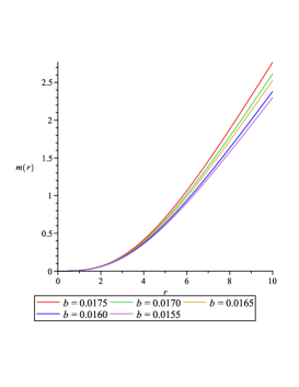
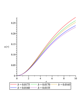
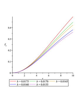
Figure 1: (Left) Variation of mass vs radial coordinate is shown in the plot for the specified range for positive flag curvature. (Middle) Variation of the compactness vs radial coordinate is shown in the plot for the specified range for positive flag curvature. (Right) Variation of the redshift vs radial coordinate is shown in the plot for the specified range for positive flag curvature.

Table 2: Maximum compactness factor, mass and surface redshift for different cases.

a	b	u(R)	m(R)	Z(R)
			(in km)
0.0216	0.0175	0.2769	2.769	0.4970
0.0225	0.0170	0.2615	2.615	0.4480
0.0226	0.0165	0.2531	2.531	0.4229
0.0236	0.0160	0.2381	2.381	0.3817
0.0237	0.0155	0.2299	2.299	0.3607

V.2 Energy Condition

Now, we verify the energy conditions namely null energy condition (NEC), weak energy condition (WEC) and strong energy condition (SEC) which can be given as follows:

$$(i)~{}NEC:\rho+p_{r}\geq 0,$$ (39)

$$(ii)~{}WEC:\rho+p_{r}\geq 0,~{}~{}\rho\geq 0,$$ (40)

$$(iii)~{}SEC:\rho+p_{r}\geq 0,~{}~{}~{}\rho+p_{r}+2p_{t}\geq 0.$$ (41)

We plot the L.H.S of the above inequalities in Fig. 3 which shows that these inequalities hold good. This therefore confirm that our model satisfies all the energy conditions.

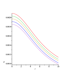
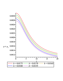
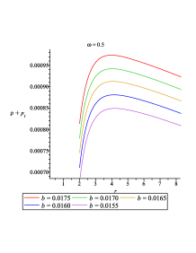
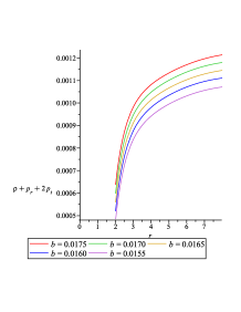
Figure 2: (Left) Variation of $\rho$ vs radial coordinate is shown in the plot for the specified range for positive flag curvature.(First Middle) Variation of $\rho+p_{r}$ vs radial coordinate is shown in the plot for the specified range for positive flag curvature. (Second Middle) Variation of $\rho+p_{t}$ vs radial coordinate is shown in the plot for the specified range for positive flag curvature. (Right) Variation of $\rho+p_{r}+2p_{t}$ vs radial coordinate is shown in the plot for the specified range for positive flag curvature.

V.3 TOV Equation

The generalized Tolman-Oppenheimer-Volkoff (TOV) equation for this system can be given by the equation Varela2010

$$-\frac{M_{G}(\rho+p_{r})}{r^{2}}\sqrt{\frac{A}{B}}-\frac{dp_{r}}{dr}+\frac{2}{r}(p_{t}-p_{r})=0,$$ (42)

where $M_{G}=M_{G}(r)$ is the effective gravitational mass inside a sphere of radius $r$ given by the Tolman-Whittaker formula which can be derived from the equation

$$M_{G}(r)=\frac{1}{2}r^{2}\frac{B^{\prime}}{\sqrt{AB}}.$$ (43)

The above equation explains the equilibrium condition of the fluid sphere due to combined effect of gravitational, hydrostatics and anisotropy forces. Equation $(34)$ can be rewritten in the following form

$$F_{g}+F_{h}+F_{a}=0,$$ (44)

where

$$F_{g}=-\frac{B^{\prime}}{2B}(\rho+p_{r}),$$ (45)

$$F_{h}=-\frac{dp_{r}}{dr},$$ (46)

$$F_{a}=\frac{2}{r}(p_{t}-p_{r}).$$ (47)

The profiles (Fig. 3) of these force indicate that the matter distribution comprising the compact star is in equilibrium state subject to the gravitational force $F_{g}$, hydrostatic force $F_{h}$ plus another force $F_{a}$ due to anisotropic pressure. The first two forces are repulsive in nature due to positivity but the later force is in attractive nature. The combined effect of these forces make the system in a equilibrium position.

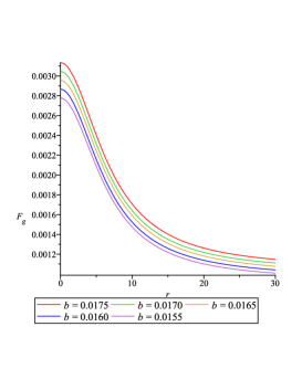
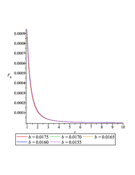
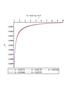
Figure 3: (Left) Variation of the gravitational force vs radial coordinate is shown in the plot for the specified range for positive flag curvature. (Middle) Variation of hydrostatics force vs radial coordinate is shown in the plot for the specified range for positive flag curvature. (Right) Variation of anisotropic force vs radial coordinate is shown in the plot for the specified range for positive flag curvature.

V.4 Stability

Now, we examine the stability of model. For this purpose, we employ the technique proposed by Herrera Herrera1992 which is known as cracking concept. At first, it requires that the squares of the radial and tangential sound speeds should be within the limit $[0,1]$. The theorem states that one can get stable configuration if radial speed of sound is greater than that of transverse speed, i.e. $v_{st}^{2}-v_{sr}^{2}$ should less than zero within the matter distribution.

Now, we calculate the radial speed ($v_{sr}$) and transverse speed ($v_{st}$) for our anisotropic model as

$$v_{sr}^{2}=\frac{dp_{r}}{d\rho}=\omega,$$ (48)

$$v^{2}_{st}=\frac{dp_{t}}{d\rho}=\frac{\alpha+\beta+\gamma}{2abr(5+ar^{2})},$$ (49)

where $\alpha=\frac{16ab\omega\lambda r-16\omega^{2}a^{2}b\lambda r^{3}+56Gwab^{2}r^{3}+6Gb^{2}r+16Gab^{2}r^{3}+6Ga^{2}b^{2}r^{5}+18G\omega^{2}b^{2}r+24G\omega^{2}ab^{2}r^{3}+6G\omega^{2}a^{2}b^{2}r^{5}+12G\omega a^{2}b^{2}r^{5}}{4(\lambda+a\lambda r^{2}-Gbr^{2})}$,

$\beta=\frac{6ar(12\omega b\lambda+8ab\omega\lambda r^{2}-4\omega^{2}a^{2}b\lambda r^{4}+14Gwab^{2}r^{4}+3Gb^{2}r^{2}+4Gab^{2}r^{4}+Ga^{2}b^{2}r^{6}+9G\omega^{2}b^{2}r^{2}+6G\omega^{2}ab^{2}r^{4}+G\omega^{2}a^{2}b^{2}r^{6}+2G\omega a^{2}b^{2}r^{6})}{4(1+ar^{2})(\lambda+a\lambda r^{2}-Gbr^{2})}$,

$\gamma=\frac{(2a\lambda r-2Gbr)(12\omega b\lambda+8ab\omega\lambda r^{2}-4\omega^{2}a^{2}b\lambda r^{4}+14Gwab^{2}r^{4}+3Gb^{2}r^{2}+4Gab^{2}r^{4}+Ga^{2}b^{2}r^{6}+9G\omega^{2}b^{2}r^{2}+6G\omega^{2}ab^{2}r^{4}+G\omega^{2}a^{2}b^{2}r^{6}+2G\omega a^{2}b^{2}r^{6})}{4(\lambda+a\lambda r^{2}-Gbr^{2})^{2}}$.

To check whether the sound speeds lie between 0 and 1 and $v_{st}^{2}-v_{sr}^{2}<0$ we plot the radial and transverse sound speeds and squares of there difference. Fig. 4 satisfies Herrera’s criterion and therefore, our model is quite stable one.

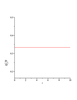
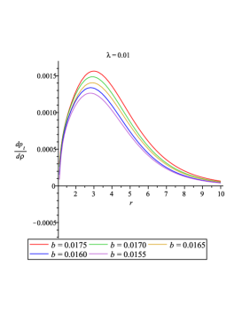
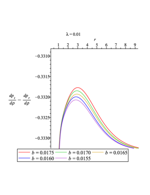
Figure 4: (Left) Variation of the square of the radial velocity vs radial coordinate is shown in the plot for the specified range for positive flag curvature. (Middle) the square of the transverse velocity. (Right) Variation of the difference between the square of the transverse velocity and square of the radial velocity vs radial coordinate is shown in the plot for the specified range for positive flag curvature.

VI CONCLUDING REMARKS

In the present investigation, we have considered anisotropic matter source for constructing a new type of solutions for compact stars. The background geometry is taken as the Finslerian structure of spacetime. It is expected that the compactness of these stars is greater than that of a neutron star. Plugging the expressions for $G$ and $c$ in the relevant equations, one can figure out that the value of the central density for the choices of the constant $b$ turn out to be $\rho_{0}\varpropto~{}10^{15}$ gm cm^-3 which is in observation relevance Ruderman1972 ; Glendenning1997 ; Herjog2011 . This result is hopeful as far as physical aspect is concerned and may be treated as a seminal bottom line of the present study.

In this same physical point of view we have studied several other physical aspects of the model to justify validity of the solutions. The features that emerge from the present investigation can be put forward as follows:

(1) Mass-radius relation: The surface redshift, which gives the compactness of the star, comes out to be in the range $0.36-0.49$ in our study. This high redshift are consistent with strange stars which have mass-radius ratios higher than neutron stars Lindblom1984 .

In this connection we were also curious about the condition of Buchdahl Buchdahl1959 related to maximum allowable mass-radius ratio limit. It is observed that Buchdahl s limit has been satisfied by our model.

(2) Energy Condition: In the present model satisfies all the energy conditions are shown to be satisfactory.

(3) TOV Equation: The generalized Tolman-Oppenheimer-Volkoff equation for the Finslerian system of compact star are studied. It has been observed that by the combined effect of the forces in action keep the system in static equilibrium.

(4) Stability: The stability of model has been examined by employing the cracking technique of Herrera Herrera1992 . We have shown via Fig. 4 that Herrera’s criterion satisfies which therefore indicates stability of our model.

As a final comment we would like to mention that the toy model as put forward in the present study for compact stars under the Finslerian structure of spacetime are seem very promising. However, some other aspects are deemed to be performed, such as issues of formation and structure of various compact stars, before one could be confirmed about the satisfactory role of the Finslerian spacetime than that of Riemannian geometry. Specifically several other issues as argued by Pfeifer and Wohlfarth Pfeifer2012 “Finsler spacetimes are viable non-metric geometric backgrounds for physics; they guarantee well defined causality, the propagation of light on a non-trivial null structure, a clear notion of physical observers and the existence of physical field theories determining the geometry of space-time dynamically in terms of an extended gravitational field equation” can be sought for in a future study.

Appendix

Let us choose $\bar{F^{2}}$ in the following form

$$\bar{F^{2}}=y^{\theta}y^{\theta}+f(\theta,\phi)y^{\phi}y^{\phi},$$

That is,

$$\bar{g}_{ij}=diag(1,f(\theta,\phi)),~{}~{}~{}~{}~{}~{}~{}and~{}~{}~{}~{}~{}\bar{g}^{ij}=diag(1,\frac{1}{f(\theta,\phi)});~{}~{}~{}~{}~{}(i,j=2,3/\theta,\phi)$$

One can find from $\bar{F^{2}}$

$$G^{2}=-\frac{1}{4}\frac{\partial f}{\partial\theta}$$

$$G^{3}=\frac{1}{4f}\left(2\frac{\partial f}{\partial\theta}y^{\phi}y^{\theta}+\frac{\partial f}{\partial\phi}y^{\phi}y^{\phi}\right)$$

Hence, one obtains

$$\bar{F}^{2}\bar{Ric}=y^{\phi}y^{\phi}\left[-\frac{1}{2}\frac{\partial^{2}f}{\partial\theta^{2}}+\frac{1}{2f}\frac{\partial^{2}f}{\partial\phi^{2}}-\frac{1}{2}\frac{\partial}{\partial\phi}\left(\frac{1}{f}\frac{\partial f}{\partial\phi}\right)-\frac{1}{4f}\left(\frac{\partial f}{\partial\theta}\right)^{2}+\frac{1}{4f}\frac{\partial f}{\partial\phi}\frac{1}{f}\frac{\partial f}{\partial\phi}+\frac{\partial f}{\partial\theta}\frac{1}{2f}\frac{\partial f}{\partial\theta}-\frac{1}{4f^{2}}\left(\frac{\partial f}{\partial\phi}\right)^{2}\right]$$

$$+y^{\theta}y^{\theta}\left[-\frac{1}{2}\frac{\partial}{\partial\theta}\left(\frac{1}{f}\frac{\partial f}{\partial\theta}\right)-\frac{1}{4f^{2}}\left(\frac{\partial f}{\partial\theta}\right)^{2}\right]+y^{\phi}y^{\theta}\left[\frac{1}{f}\frac{\partial^{2}f}{\partial\theta\partial\phi}-\frac{1}{2}\frac{\partial}{\partial\theta}\left(\frac{1}{f}\frac{\partial f}{\partial\phi}\right)-\frac{1}{2}\frac{\partial}{\partial\phi}\left(\frac{1}{f}\frac{\partial f}{\partial\theta}\right)\right]$$

Now, coefficient of $y^{\phi}y^{\theta}=0$ iff, $f$ is independent of $\phi$ i.e.

$$f(\theta,\phi)=f(\theta)$$

( but coefficient of $y^{\theta}y^{\theta}$ $\&$ $y^{\phi}y^{\phi}$ are non zero )

Therefore,

$$\bar{F}^{2}\bar{Ric}=\left[-\frac{1}{2f}\frac{\partial^{2}f}{\partial\theta^{2}}+\frac{1}{4f^{2}}\left(\frac{\partial f}{\partial\theta}\right)^{2}\right](y^{\theta}y^{\theta}+fy^{\phi}y^{\phi})$$

Hence,

$$\bar{Ric}=-\frac{1}{2f}\frac{\partial^{2}f}{\partial\theta^{2}}+\frac{1}{4f^{2}}\left(\frac{\partial f}{\partial\theta}\right)^{2}=\lambda$$

Here, $\lambda$ may be a constant or a function of $\theta$.

Putting, $\frac{1}{f}\left(\frac{\partial f}{\partial\theta}\right)=T(\theta)$, the above equation yields

$$\frac{dT}{d\theta}+\frac{1}{2}T^{2}+2\lambda=0$$

For constant $\lambda$, one can get Finsler structure $\bar{F^{2}}$ as

$$\bar{F}^{2}=y^{\theta}y^{\theta}+A\sin^{2}(\sqrt{\lambda}\theta)y^{\phi}y^{\phi},~{}~{}\lambda>0$$

$$=y^{\theta}y^{\theta}+A\theta^{2}y^{\phi}y^{\phi},~{}~{}\lambda=0$$

$$=y^{\theta}y^{\theta}+A\sinh^{2}(\sqrt{-\lambda}\theta)y^{\phi}y^{\phi},~{}~{}\lambda<0$$

[ A may be taken as 1 ]

Now, the Finsler structure takes the form

$${F}^{2}=B(r)y^{t}y^{t}-A(r)y^{r}y^{r}-r^{2}y^{\theta}y^{\theta}-r^{2}\sin^{2}\theta y^{\phi}y^{\phi}+r^{2}\sin^{2}\theta y^{\phi}y^{\phi}-r^{2}\sin^{2}(\sqrt{\lambda}\theta)y^{\phi}y^{\phi}$$

$$=\alpha^{2}+r^{2}(\sin^{2}\theta-\sin^{2}(\sqrt{\lambda}\theta))y^{\phi}y^{\phi}~{}~{}~{}~{}~{}~{}~{}~{}~{}~{}~{}~{}~{}~{}~{}~{}~{}~{}~{}~{}~{}~{}~{}~{}~{}~{}~{}~{}~{}~{}~{}~{}~{}~{}~{}~{}~{}~{}~{}~{}~{}~{}~{}~{}~{}~{}~{}~{}$$

$$=\alpha^{2}+r^{2}\chi(\theta)y^{\phi}y^{\phi}~{}~{}~{}~{}~{}~{}~{}~{}~{}~{}~{}~{}~{}~{}~{}~{}~{}~{}~{}~{}~{}~{}~{}~{}~{}~{}~{}~{}~{}~{}~{}~{}~{}~{}~{}~{}~{}~{}~{}~{}~{}~{}~{}~{}~{}~{}~{}~{}~{}~{}~{}~{}~{}~{}~{}~{}~{}~{}~{}~{}~{}~{}~{}~{}~{}~{}~{}$$

where $\chi(\theta)=\sin^{2}\theta-\sin^{2}(\sqrt{\lambda}\theta)$.

Thus,

$${F}=\alpha\sqrt{1+\frac{r^{2}\chi(\theta)y^{\phi}y^{\phi}}{\alpha^{2}}}$$

Let, $b_{\phi}=r\sqrt{\chi(\theta)}$, then

$${F}=\alpha\sqrt{1+\frac{(b_{\phi}y^{\phi})^{2}}{\alpha^{2}}}=\alpha\sqrt{1+s^{2}}$$

where,

$$s=\frac{(b_{\phi}y^{\phi})}{\alpha}=\frac{\beta}{\alpha}$$

$$b_{\mu}=(0,0,0,b_{\phi})~{},~{}~{}b_{\phi}y^{\phi}=b_{\mu}h^{\mu}=\beta~{},~{}(\beta~{}is~{}one~{}form)$$

Finally, we have

$$F=\alpha\phi(s)~{}~{},~{}~{}\phi(s)=\sqrt{1+s^{2}}$$

Hence, F is the metric of $(\alpha,\beta)$-Finsler space.

The killing equation $K_{V}(F)=0$ in Finsler space can be obtained by considering the isometric transformations of Finsler structure XL . One can investigate the Killing vectors of $(\alpha,\beta)$ - Finsler space. The Killing equations for this class of Finsler space is given as

$$\left(\phi(s)-s\frac{\partial\phi(s)}{\partial s}\right)K_{V}(\alpha)+\frac{\partial\phi(s)}{\partial s}K_{V}\beta)=0,$$

where

$$K_{V}(\alpha)=\frac{1}{2\alpha}\left(V_{\mu\mid\nu}+V_{\nu\mid\mu}\right)y^{\mu}y^{\nu},$$

$$K_{V}(\beta)=\left(V^{\mu}\frac{\partial b_{\nu}}{\partial x^{\mu}}+b_{\mu}\frac{\partial V^{\mu}}{\partial x^{\nu}}\right)y^{\nu}.$$

Here $"\mid"$ represents the covariant derivative with respect to the Riemannian metric $\alpha$. For the present case of Finsler structure it is given by

$$K_{V}(\alpha)+sK_{V}(\beta)=0~{}~{}or~{}~{}\alpha K_{V}(\alpha)+\beta K_{V}(\beta)=0.$$

Consequently, we have the solution

$$K_{V}(\alpha)=0~{}~{}and~{}~{}K_{V}(\beta)=0$$

or

$$V_{\mu\mid\nu}+V_{\nu\mid\mu}=0$$

and

$$V^{\mu}\frac{\partial b_{\nu}}{\partial x^{\mu}}+b_{\mu}\frac{\partial V^{\mu}}{\partial x^{\nu}}=0.$$

It is to be noted that the second Killing equation constrains the first one which is, in fact, the Killing equation of the Riemannian space, that is, it is responsible for breaking the symmetry (isometric) of the Riemannian space.

On the othe hand, the Finsler space we are considering is , in fact, can be determined from a Riemannian manifold $(M,g_{\mu\nu}(x))$ as we have

$$F(x,y)=\sqrt{g_{\mu\nu}(x)y^{\mu}y^{\nu}}$$

( cf. equations (5) and (6) in the case $\bar{F^{2}}$ is quadric in $y^{\theta}~{}\&~{}y^{\phi}$ )

It is a semi-definite Finsler space. Therefore, we can take covariant derivative of the Riemanian space. The Bianchi identities are, in fact, coincident with those of the Riemanian space (being the covariant conservation of Einstein tensor). The present Finsler space is reducible to the Riemanian space and consequently the gravitational field equations can be obtained. Also we shall find the gravitational field equations alternatively following XC . They have also shown the covariantly conserved properties of the tensor $G^{\mu}_{\nu}$ in respect of covariant derivative in Finsler spacetime with the Chern-Rund connection. Presently this conserved property of $G^{\mu}_{\nu}$ which are, in fact, in the same forms but obtained from the Riemanian manifold follows by using the covariant derivative of that space (which are, in fact, the Bianchi identity). Also we point out the gravitational field equation (18) is restricted to the base manifold of the Finsler space, as in XL , and the fiber coordinates $y^{i}$ are set to be the velocities of the cosmic components (velocities in the energy momentum tensor). Also, Xin Li, et al. XL have shown that there gravitational field equation could be derived from the of Pfeifer et.al. approximately Pf . Pfeifer et.al. Pf have constructed gravitational dynamic for Finsler spacetime in terms of an action integral on the unit tangent bundle. Also the gravitational field equation (18) is insensitive to the connection because $G_{\nu}^{\mu}$ are obtained from the Ricci scalar which is in fact, insensitive to the connections and depend only on the Finsler structure F.

Thus the above equations(20)-(22) are derived from the modified gravitational field equation (18) taking anisotropic energy momentum tensor (19) as well as these equations are derivable from the Einstein gravitational field equation in the Riemannian spacetime with the metric (6) in which the metric $\bar{g}_{ij}$ is given by

$$\bar{g}_{ij}=diag~{}(~{}1~{},~{}~{}\sin^{2}\sqrt{\lambda}\theta~{})$$

That is,

$$g_{\mu\nu}=diag~{}(~{}B,~{}-A,~{}-r^{2}~{},~{}~{}-r^{2}\sin^{2}\sqrt{\lambda}\theta~{})$$

$$g^{\mu\nu}=diag~{}(~{}B^{-1},~{}-A^{-1},~{}-r^{-2}~{},~{}~{}-r^{-2}\sin^{-2}\sqrt{\lambda}\theta~{})$$

The terms involving $\lambda$ in these equations are playing the physically meaning role doing the effect of the Finsler geometric consideration of the problem.

References

- (1) A. Pais, Subtle is the Lord: The Science and Life of Albert Einstein (Oxford Univ. Press, 1982).
- (2) W. Baade and F. Zwicky, Physical Review, 46, 76 (1934).
- (3) M.S. Longair, High Energy Astrophysics (Vol. 2, Cambridge Univ., p.99, 1994).
- (4) P. Ghosh, Rotation and Accretion Powered Pulsars (p.2, World Scientific, 2007).
- (5) R. Ruderman, Rev. Astr. Astrophys. 10, 427 (1972).
- (6) M.K. Gokhroo, A.L. Mehra, Gen. Relativ. Grav. 26, 75 (1994).
- (7) R. Kippenhahn, A. Weigert, Steller Structure and Evolution (Springer-Verlag, 1990).
- (8) A.I. Sokolov, JETP 79, 1137 (1980).
- (9) R.F. Sawyer, Phys. Rev. Lett. 29, 382 (1972); Erratum Phys. Rev. Lett. 29, 823 (1972).
- (10) H.O. Silva et al., arXiv: 1411.6286 (2014).
- (11) R.L. Bowers, E.P.T. Liang, Astrophys. J. 188, 657 (1917).
- (12) L. Herrera, A. Di Prisco, J. Martin, J. Ospino, N.O. Santos, O. Troconis, Phys. Rev. D 69, 084026, (2004).
- (13) V. Varela, F. Rahaman, S. Ray, K. Chakraborty, M. Kalam, Phys. Rev. D 82, 044052 (2010).
- (14) F. Rahaman, S. Ray, A.K. Jafry, K. Chakraborty, Phys. Rev. D 82, 104055 (2010).
- (15) F. Rahaman, R. Sharma, S. Ray, R. Maulick, I. Karar, Eur. Phys. J. C 72, 2071 (2012).
- (16) F. Rahaman, R. Maulick, A.K. Yadav, S. Ray, R. Sharma, Gen. Rel. Grav. 44, 107 (2012).
- (17) M. Kalam, F. Rahaman, S. Ray, M. Hossein, I. Karar, J. Naskar, Euro. Phys. J. C 72, 2248 (2012).
- (18) Sk. M. Hossein, F. Rahaman, J. Naskar, M. Kalam, S. Ray, Int. J. Mod. Phys. D 21, 1250088 (2012).
- (19) M. Kalam, A.A. Usmani, F. Rahaman, S.M. Hossein, I. Karar, R. Sharma, Int. J. Theor. Phys. 52, 3319 (2013).
- (20) L. Herrera, N.O. Santos, Phys. Report. 286, 53 (1997).
- (21) D. Bao, S. S. Chern, and Z. Shen, An Introduction to Riemann Finsler Geometry, Graduate Texts in Mathematics (Springer, New York, 2000).
- (22) E. Cartan, Les Espaces de Finsler (Paris, Herman, 1935).
- (23) J. I. Horv th, Phys. Rev. 80 (1950) 2001.
- (24) S. Vacaru, Int. J. Mod. Phys. D 21 (2012) 1250072; arXiv: 1004.3007.
- (25) S. Vacaru, Critical remarks on Finsler modifications of gravity and cosmology by Zhe Chang and Xin Li, Phys. Lett. B 690 (2010) 224-228; arXiv: 1003.0044v2.
- (26) S. Vacaru, Nucl. Phys. B, 434 (1997) 590 -656; arXiv: hep-th/9611034.
- (27) S. Vacaru, J. Math. Phys. 37 (1996) 508-523.
- (28) S. Vacaru, Gener. Relat. Grav. 44 (2012) 1015-1042; arXiv: 1010.5457.
- (29) S. Rajpoot and S. Vacaru, Int. J. Geom. Meth. Mod. Phys. 12 (2015); arXiv: 1506.08696.
- (30) P. Stavrinos and S. Vacaru, Class. Quant. Grav. 30 (2013) 055012; arXiv: 1206.3998
- (31) C. Lämmerzahl, V. Perlick and W. Hasse, Phys. Rev. D, 86, 104042 (2012).
- (32) D.G. Pavlov, AIP Conf. Proc. 1283, 180 (2010).
- (33) S.I. Vacaru, Class. Quantum Gravit. 27, 105003 (2010).
- (34) X. Li and Z. Chang, Phys. Rev. D, 90, 064049 (2014).
- (35) H. Akbar-Zadeh, Acad. Roy. Belg. Bull. Cl. Sci., 74, 281 (1988).
- (36) F. Rahaman et al., Phys. Rev. D, 82, 104055 (2010).
- (37) M.R. Finch and J.E.F. Skea, Class. Quantum Grav., 6, 467 (1989).
- (38) F.S.N. Lobo, Class. Quantum Grav., 23, 1525 (2006).
- (39) M.K. Mak and T. Harko, Proc. Roy. Soc. Lond., A459, 393 (2003).
- (40) R. Sharma and S. Maharaj, MNRAS, 375, 1265 (2007).
- (41) H.A. Buchdahl, Phys. Rev., 116, 1027 (1959).
- (42) L. Lindblom, Astrophys. J., 278, 364 (1984).
- (43) L. Herrera, Phys. Lett. A, 165, 206 (1992).
- (44) N.K. Glendenning, Compact Stars: Nuclear Physics, Particle Physics and General Relativity (Springer-Verlag, New York, p. 70, 1997).
- (45) M. Herjog and F.K. Roepke, arXiv: 1109.0539 [astro-ph.HE] (2014).
- (46) C. Pfeifer and M. Wohlfarth, Proceedings of the MG13 Meeting on General Relativity, Stockholm University, Sweden, 1 - 7 July (2012), doi: 10.1142/9789814623995_0094
- (47) Xin Li et al, arxiv: 1309.1758.
- (48) Xin Li Z Chang, arXiv:1401.6363.
- (49) C.Pfeifer and M.N.R. Wohlfarth, Phys. Rev. D 85,064009(2012).