Abstract. Multiple Schramm-Loewner Evolutions (SLE) are conformally invariant random processes of several curves, whose construction by growth processes relies on partition functions — Möbius covariant solutions to a system of second order partial differential equations. In this article, we use a quantum group technique to construct a distinguished basis of solutions, which conjecturally correspond to the extremal points of the convex set of probability measures of multiple $\mathrm{SLE}$s.

1. Introduction

In the 1980s, it was recognized that conformal symmetry should emerge in the scaling limits of two-dimensional models of statistical physics at critical points of continuous phase transitions [BPZ84, Car88]. This belief has provided an important motivation for remarkable developments in conformal field theories (CFT) during the past three decades. Especially in the past fifteen years, also progress in rigorously controlling scaling limits of lattice models and showing their conformal invariance has been made. Some such results concern correlations of local fields as in CFT [Ken00, Hon10, HS13, CHI15] or more general observables [Smi01, CS12, CI13], but the majority has been formulated in terms of random interfaces in the models [LSW04, CN07, Zha08a, HK13, CDCH⁺14, Izy15, Izy16].

The focus on interfaces and random geometry in general was largely inspired by the seminal article [Sch00] of Schramm. Schramm observed that if scaling limits of random interfaces between two marked boundary points of simply connected domains satisfy two natural assumptions, conformal invariance and domain Markov property, the limit must fall into a one-parameter family of random curves. The parameter $\kappa>0$ is the most important characteristic of such interfaces, and the corresponding curves are known as chordal $\mathrm{SLE}_{\kappa}$, an abbreviation for Schramm-Loewner Evolution. This classification result is sometimes referred to as Schramm’s principle.

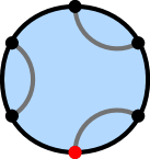
The simplest setup for Schramm’s principle is the chordal case described above: a simply connected domain $\Lambda$ with a curve connecting two marked boundary points $\xi,\eta\in\partial\Lambda$. This setup arises in models of statistical mechanics when opposite boundary conditions are imposed on two complementary arcs $\overline{\xi\eta}$ and $\overline{\eta\xi}$ of the domain boundary $\partial\Lambda$, forcing the existence of an interface between $\xi$ and $\eta$. Some variations of the chordal $\mathrm{SLE}$ setup are obtained if one considers one marked point on the boundary and another in the bulk, which leads to radial $\mathrm{SLE}$ [Sch00, RS05], or three marked boundary points, which leads to dipolar $\mathrm{SLE}$ [Zha04, BBH05]. For the purposes of statistical mechanics, one of the most natural generalizations involves dividing the boundary to an even number $2N$ of arcs, and imposing alternating boundary conditions of opposite type on the arcs. This forces interfaces to start at $2N$ marked boundary points, and such interfaces will connect the points pairwise without crossing. In this situation, one has $N$ random interfaces, see Figure 1.1. Such generalizations of $\mathrm{SLE}$-type processes have been considered in [BBK05, Gra07, Dub07], and they are generally termed multiple $\mathrm{SLE}$s or $N$-$\mathrm{SLE}$s. Results about convergence of lattice model interfaces to multiple $\mathrm{SLE}$s have been obtained in [CS12, Izy11].

Classification of multiple $\mathrm{SLE}$s by partition functions

Multiple $\mathrm{SLE}$s should still satisfy conformal invariance and domain Markov property. An important difference arises, however, when a classification along the lines of Schramm’s principle is attempted. While any configuration of a simply connected domain with two marked boundary points $(\Lambda;\xi,\eta)$ can be conformally mapped to any other according to Riemann mapping theorem, the same no longer holds with configurations $(\Lambda;\xi_{1},\ldots,\xi_{2N})$ of a domain with $2N$ marked boundary points for $N\geq 2$ — such configurations have nontrivial conformal moduli. The requirement of conformal invariance is therefore less restrictive, and one should expect to find a larger family of random processes of $N$ curves. These processes form a convex set, as one can randomly select between given possibilities. A natural suggestion was put forward in [BBK05]: the extremal points of this convex set should be processes which have a deterministic pairwise connectivity of the $2N$ boundary points by the $N$ non-crossing curves in the domain. Such extremal processes were termed pure geometries of multiple $\mathrm{SLE}$s. Pure geometries of multiple $\mathrm{SLE}$s are thus labeled by non-crossing connectivities, or equivalently, planar pair partitions $\alpha$. For fixed $N$, the number of them is the Catalan number $\mathrm{C}_{N}=\frac{1}{N+1}\binom{2N}{N}$.

               
               

Figure 1.1. In statistical mechanics models with alternating boundary conditions on $2N$ boundary segments, interfaces form one of the $\mathrm{C}_{N}$ possible planar connectivities. The figure exemplifies the $N=3$ case with critical Ising model simulations in a $100\times 100$ square. Such critical Ising interfaces tend to multiple $\mathrm{SLE}_{\kappa}$ with $\kappa=3$ in the scaling limit [Izy11, Izy16].

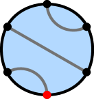
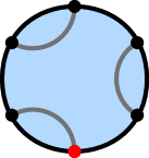
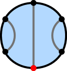
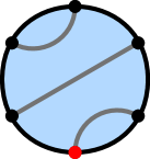
This article pertains to an explicit description and construction of the pure geometries of multiple $\mathrm{SLE}$s. We follow the approach of [Dub07, BBK05, Gra07, Dub06], in which local multiple $\mathrm{SLE}$s are constructed by growth processes of the curves starting from the marked points $\xi_{1},\ldots,\xi_{2N}\in\partial\Lambda$. The probabilistic details are postponed to Appendix A, where we give the precise definition of local multiple $\mathrm{SLE}$s, the ingredients of their construction and classification, as well as relevant properties. Crucially, the construction of a local $N$-$\mathrm{SLE}_{\kappa}$ uses a partition function, a function $\mathcal{Z}$ defined on the chamber

(1.1) $$\mathfrak{X}_{2N}=\; \left\{(x_{1},\ldots,x_{2N})\in\mathbb{R}^{2N}\;\Big{|}\;x_{1}<\cdots<x_{2N}\right\}.$$

The partition function $\mathcal{Z}$ is subject to a number of requirements. First of all, it should be positive, $\mathcal{Z}(x_{1},\ldots,x_{2N})>0$, since it is used in expressing the Radon-Nikodym derivatives of initial segments of the local $N$-$\mathrm{SLE}_{\kappa}$ curves with respect to ordinary chordal $\mathrm{SLE}$s. It has to satisfy a system of $2N$ linear partial differential equations (PDE) of second order,

(1.2) $$\left[\frac{\kappa}{2}\frac{\partial^{2}}{\partial x_{i}^{2}}+\sum_{j\neq i}\left(\frac{2}{x_{j}-x_{i}}\frac{\partial}{\partial x_{j}}-\frac{2h}{(x_{j}-x_{i})^{2}}\right)\right]\mathcal{Z}(x_{1},\ldots,x_{2N})=0\qquad\text{for all }i=1,\ldots,2N,$$

where $h=\frac{6-\kappa}{2\kappa}$, to guarantee a stochastic reparametrization invariance [Dub07]. It has to transform covariantly (COV) under Möbius transformations $\mu(z)=\frac{az+b}{cz+d}$,

(1.3) $$\mathcal{Z}(x_{1},\ldots,x_{2N})=\; \prod_{i=1}^{2N}\mu^{\prime}(x_{i})^{h}\times\mathcal{Z}(\mu(x_{1}),\ldots,\mu(x_{2N})),$$

in order for the constructed process to be invariant under conformal self-maps of the simply connected domain $\Lambda$. The results of Appendix A state that local multiple $\mathrm{SLE}$s are classified by such partition functions $\mathcal{Z}$, and the convex structure of the multiple $\mathrm{SLE}$s corresponds to the convex structure of the set of such functions.

Theorem (Theorem A.4).

• Any partition function $\mathcal{Z}$ can be used to construct a local multiple $\mathrm{SLE}_{\kappa}$, and two functions $\mathcal{Z},\tilde{\mathcal{Z}}$ give rise to the same local multiple $\mathrm{SLE}_{\kappa}$ if and only if they are constant multiples of each other.

• Any local multiple $\mathrm{SLE}_{\kappa}$ can be constructed from some partition function $\mathcal{Z}$, which is unique up to a multiplicative constant.

• For any $\,0\leq r\leq 1\,$, if $\mathcal{Z}=r\,\mathcal{Z}_{1}+(1-r)\,\mathcal{Z}_{2}$ is a convex combination of two partition functions $\mathcal{Z}_{1}$ and $\mathcal{Z}_{2}$, then the local multiple $\mathrm{SLE}_{\kappa}$ probability measures associated to $\mathcal{Z}$ are convex combinations of the probability measures associated to $\mathcal{Z}_{1}$ and $\mathcal{Z}_{2}$, with coefficients proportional to $r$ and $1-r$, and proportionality constants depending on the conformal moduli of the domain with the marked points.

Multiple $\mathrm{SLE}$ pure partition functions

The above results form a general classification of local multiple $\mathrm{SLE}$s by the solution space of the system (1.2) – (1.3). This solution space can be shown to be finite dimensional [Dub06], and indeed, the correct dimension $\mathrm{C}_{N}$ has been established in the articles [FK15a, FK15b, FK15c] (for solutions with at most polynomial growth rate at diagonals and infinity).

The task is to construct multiple $\mathrm{SLE}$ pure geometries, for each possible connectivity of the $N$ curves. The sequence of marked boundary points $\xi_{1},\ldots,\xi_{2N}$ is from now on assumed to appear in a positive (counterclockwise) order along the boundary $\partial\Lambda$. We encode the connectivities of the non-crossing curves by planar pair partitions $\alpha$ of the indices $1,\ldots,2N$ of the marked points $\xi_{1},\ldots,\xi_{2N}$. As has become standard in the literature, we refer to the pairs as links and the pair partitions as link patterns. A link formed by the pair $\left\{a,b\right\}$ of indices will be denoted by $[\wideparen{a,b}]$. A link pattern will be denoted by

$$\alpha=\left\{[\wideparen{a_{1},b_{1}}],\ldots,[\wideparen{a_{N},b_{N}}]\right\}.$$

The non-crossing condition, i.e., the planar property of the pair partition, can be expressed as the requirement $(a_{j}-a_{k})(b_{j}-b_{k})(b_{j}-a_{k})(a_{j}-b_{k})>0$ whenever $j\neq k$. The set of link patterns of $N$ links is denoted by $\mathrm{LP}_{N}$, and we recall that the number of these is a Catalan number, $\#\mathrm{LP}_{N}=\mathrm{C}_{N}=\frac{1}{N+1}\binom{2N}{N}$. By convention, we include the empty link pattern $\emptyset\in\mathrm{LP}_{0}$ in the case $N=0$. The set of link patterns of any possible size is denoted by $\mathrm{LP}=\bigsqcup_{N\geq 0}\mathrm{LP}_{N}$, and for $\alpha\in\mathrm{LP}_{N}$, we denote $|\alpha|=N.$

We seek pure geometries of multiple $\mathrm{SLE}$s corresponding to each link pattern, so in view of the theorem above, the task is to construct their corresponding partition functions $(\mathcal{Z}_{\alpha})_{\alpha\in\mathrm{LP}}$. Each $\mathcal{Z}_{\alpha}$ must solve the system (1.2) – (1.3). This system, which is the same for all link patterns $\alpha$ of the same number of links, is supplemented by boundary conditions which depend on $\alpha$.

The boundary conditions are stated in terms of removing links from the link pattern. After removal of one link from $\alpha\in\mathrm{LP}_{N}$, the indices must be relabeled by $1,\ldots,2N-2$. When $[\wideparen{j,j+1}]\in\alpha$, we denote by $\alpha/[\wideparen{j,j+1}]$ the link pattern of $N-1$ links where the link $[\wideparen{j,j+1}]$ is removed and indices greater than $j+1$ are reduced by two, see Figure 1.2.

Figure 1.2. When removing the link $[\wideparen{3,4}]$ from the link pattern $\alpha=\left\{[\wideparen{1,8}],[\wideparen{2,5}],[\wideparen{3,4}],[\wideparen{6,7}]\right\}\in\mathrm{LP}_{4}$, we obtain $\alpha/[\wideparen{3,4}]=\left\{[\wideparen{1,6}],[\wideparen{2,3}],[\wideparen{4,5}]\right\}\in\mathrm{LP}_{3}$ after relabeling the remaining endpoints.

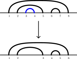
The boundary conditions are recursive in the number of links: the conditions for $\mathcal{Z}_{\alpha}$, $\alpha\in\mathrm{LP}_{N}$, depend on the solutions $\mathcal{Z}_{\hat{\alpha}}$, $\hat{\alpha}\in\mathrm{LP}_{N-1}$. Specifically, we require of $\mathcal{Z}_{\alpha}$ that for all $j=1,\ldots,2N-1$ and any $\xi\in(x_{j-1},x_{j+2})$, we have

(1.4) $$\lim_{x_{j},x_{j+1}\to\xi}\frac{\mathcal{Z}_{\alpha}(x_{1},\ldots,x_{2N})}{(x_{j+1}-x_{j})^{-2h}}=\; \begin{cases}0\quad&\text{if }[\wideparen{j,j+1}]\notin\alpha\\ \mathcal{Z}_{\alpha/[\wideparen{j,j+1}]}(x_{1},\ldots,x_{j-1},x_{j+2},\ldots,x_{2N})&\text{if }[\wideparen{j,j+1}]\in\alpha.\end{cases}$$

These conditions were proposed in [BBK05], where pure geometries were introduced, and they were conjectured to be sufficient to determine a solution to the system (1.2) – (1.3). The probabilistic meaning of these conditions is clarified in Appendix A, Propositions A.5 and A.6. Solutions to the system (1.2) – (1.4) will be called multiple $\mathrm{SLE}$ pure partition functions. The collection $(\mathcal{Z}_{\alpha})_{\alpha\in\mathrm{LP}}$ solving these conditions turns out to be unique up to one multiplicative factor, and although positivity is neither required nor proved here, we conjecture that the factor can be chosen so that all $\mathcal{Z}_{\alpha}$ are simultaneously positive.

The main result of this article is the explicit construction of these Möbius covariant solutions to the system of PDEs with boundary conditions. The statement concerns the physically relevant parameter range $\kappa\leq 8$, and generic values $\kappa\notin\mathbb{Q}$, which avoids certain algebraic and analytic degeneracies.

Theorem (Theorem 4.1).

For $\kappa\in(0,8)\setminus\mathbb{Q}$, there exists a collection $\left(\mathcal{Z}_{\alpha}\right)_{\alpha\in\mathrm{LP}}$ of functions

$$\mathcal{Z}_{\alpha}\;\colon\;\mathfrak{X}_{2|\alpha|}\rightarrow\mathbb{C}$$

such that the system of equations (1.2) – (1.4) holds for all $\alpha\in\mathrm{LP}$. For any $N\in\mathbb{Z}_{\geq 0}$, the collection $\left(\mathcal{Z}_{\alpha}\right)_{\alpha\in\mathrm{LP}_{N}}$ is linearly independent and it spans a $\mathrm{C}_{N}$-dimensional space of solutions to (1.2) – (1.3).

Our solution is based on a systematic quantum group technique developed in [KP14]. By the “spin chain – Coulomb gas correspondence” of that article, we translate the problem of solving the system (1.2) – (1.4) to a linear problem in a $2^{N}$-dimensional representation of a quantum group, the $q$-deformation of $\mathfrak{sl}_{2}$. With this translation, we first exhibit an explicit formula for all maximally nested (rainbow) link patterns, and then obtain the solutions for other link patterns using a recursion on the partially ordered set of link patterns with a given number $N$ of links.

Solutions to $\mathrm{SLE}$ boundary visit amplitudes

Using our solution to the problem of multiple $\mathrm{SLE}$ pure partition functions, we also derive the existence of solutions to another question to which the “spin chain – Coulomb gas correspondence” is applied — the chordal $\mathrm{SLE}$ boundary visit amplitudes, treated in [JJK16]. These amplitudes are functions indexed by possible orders of visits, $\mathrm{VO}=\bigsqcup_{N^{\prime}\in\mathbb{N}}\mathrm{VO}_{N^{\prime}}$, where $\mathrm{VO}_{N^{\prime}}=\left\{-,+\right\}^{N^{\prime}}$ is the set of possible orders of visits to $N^{\prime}$ boundary points. Like multiple $\mathrm{SLE}$ pure partition functions, the boundary visit amplitudes $\left(\zeta_{\omega}\right)_{\omega\in\mathrm{VO}}$ are required to satisfy partial differential equations, covariance (translation invariance and homogeneity), and boundary conditions (prescribed asymptotic behaviors). We postpone the precise statement of the problem to Section 5. Uniqueness of solutions in the class of functions obtained by the “spin chain – Coulomb gas correspondence” is relatively easy, and existence was shown for $N^{\prime}\leq 4$ in [JJK16] by direct calculations. We prove the existence for all $N^{\prime}$.

Theorem (Theorem 5.2).

For $\kappa\in(0,8)\setminus\mathbb{Q}$, there exists a collection $\left(\zeta_{\omega}\right)_{\omega\in\mathrm{VO}}$ of functions such that the system of partial differential equations, covariance, and boundary conditions required in [JJK16] holds for all $\omega\in\mathrm{VO}$.

Relation to other work

We follow the approach of constructing multiple $\mathrm{SLE}$s by a growth process, where a partition function $\mathcal{Z}$ is needed as an input. An alternative approach is the so called configurational measure of multiple $\mathrm{SLE}$s, where the Radon-Nikodym derivative of the law of the full global configuration of curves (w.r.t. $N$ chordal $\mathrm{SLE}$s) is written in terms of Brownian loop measure. For $\kappa\leq 4$, the configurational measures for the maximally nested (rainbow) link patterns were constructed in [KL07]. However, constructions of configurational measures with $4<\kappa\leq 8$ have not been given. The most obvious advantage of the configurational measure is the direct treatment of the global configuration. In contrast, the growth process construction straightforwardly only allows to define localized versions of multiple $\mathrm{SLE}$s (see Appendix A), and the extension to globally defined random curves poses challenges similar to the reversibility of chordal $\mathrm{SLE}$ [Zha08b, MS12b]. The partition function approach, however, is somewhat more explicit and better suited for example for sampling multiple $\mathrm{SLE}$s. The two approaches should of course produce the same results, and in a future work we plan to show this. The total masses of the unnormalized configurational measures will, in particular, be explicitly expressible in terms of our partition functions.

The pure partition functions are intimately related to crossing probabilities in models of statistical physics [BBK05], and they have also been called “connectivity weights” in the literature [FK15d, FSK15]. Note that for $N=2$, Möbius covariance (1.3) allows to reduce the partial differential equations (1.2) to ordinary differential equations, and pure partition functions for $2$-SLE are then straightforwardly solvable in terms of hypergeometric functions [BBK05]. They generalize Cardy’s formula [Car92] for crossing probabilities for critical percolation, to which they reduce at $\kappa=6$. For percolation and $N=3$, a recent numerical study [FZS15] confirms the validity of crossing probability formulas found in [Sim13]. Very recently, explicit formulas for connectivity weights for cases $N=3$ and $N=4$ and a formula for rainbow connectivity weights for general $N$ were worked out in [FSK15]. Virtually all work for $N>2$ relies on some form of Coulomb gas integral solutions [DF84], which also underlie the correspondence [KP14] that is crucially employed in the present work.

The solutions to the system (1.2) – (1.3) for all $N$ have also been studied in the series of articles [FK15a, FK15b, FK15c, FK15d]. The main results are closely parallel to ours, although the works have been independent. Our integrals treat all marked points symmetrically at the expense of having dimension one higher than those of Flores and Kleban. Importantly, by different analytic methods, Flores and Kleban prove also the upper bound for the dimension of the solution space, and by a limiting procedure, they obtain results about rational $\kappa$.

We include a probabilistic justification for the system (1.2) – (1.3) and boundary conditions (1.4), in the form of a classification and properties of local multiple $\mathrm{SLE}$s, in Appendix A. Our method of solving this system has the advantage of being completely systematic, in translating the problem to algebraic calculations in finite dimensional representations of a quantum group. The translation, based on [KP14], allows to deduce properties of the solutions conceptually, using representation theory. This systematic formalism will also be valuable in further applications, which require establishing for example bounds or monodromy properties of the solutions.

In [JJK16], the quantum group method of [KP14] was applied to formulas for the probability that a chordal $\mathrm{SLE}$ curve passes through small neighborhoods of given points on the boundary. Solutions were given for cases having up to four visited points. In Section 5, we present a solution for arbitrary number of visited points, making use of natural representation theoretic mappings to reduce the problem to the main results of this article.

Related questions of random connectivities in planar non-crossing ways appear also in various other interesting contexts. Notably, the famous Razumov-Stroganov conjecture has a reformulation in terms of probabilities of the different planar connectivities alternatively in a percolation model on a semi-infinite lattice cylinder, or in a fully packed loop model in a lattice square [RS04, CS11]. As another example, the boundary conditions that enforce the existence of $N$ interfaces connecting $2N$ boundary points can be studied in models of statistical mechanics on random lattices, i.e., in discretized quantum gravity. Partition functions of the various connectivities for the Ising model on random lattices have been found by matrix model techniques in [EO05]. In both of the above mentioned problems, some relations to the present work can be anticipated, since conformal field theory is expected to underlie each of the models. Unveiling precise connections to these, however, is left for future research.

Organization of the article

In Section 2, we give the definition of the quantum group $\mathcal{U}_{q}(\mathfrak{sl}_{2})$, summarize needed facts about its representation theory, and present a special case of the “spin chain – Coulomb gas correspondence”, which is our main tool in the construction of multiple $\mathrm{SLE}$ partition functions. Section 3 contains the solution of a quantum group reformulation of the problem of multiple $\mathrm{SLE}$ pure partition functions. In Section 4, with the help of the correspondence of Section 2, this solution is translated to the construction of the pure partition functions. We also discuss symmetric partition functions relevant for models invariant under cyclic permutations of the marked points, and give examples of such symmetric partition functions for the Ising model, Gaussian free field, and percolation.

Section 5 is devoted to the proof of the existence of solutions to the $\mathrm{SLE}$ boundary visit problem. Finally, in Appendix A, we include an account of the probabilistic aspects: the classification and construction of local multiple $\mathrm{SLE}$s by partition functions, and the role of the requirements (1.2) – (1.4).

Acknowledgments

K. K. is supported by the Academy of Finland, and E. P. by Vilho, Yrjö and Kalle Väisälä Foundation. During this work, we have benefited from interesting discussions with Steven Flores, Clément Hongler, Yacine Ikhlef, Kostya Izyurov, Peter Kleban, Michael Kozdron, Greg Lawler, and Jake Simmons.

2. The quantum group method

In this section, we present the quantum group method in the form it will be used for the solution of the problem (1.2) – (1.4). The method was developed more generally in [KP14].

The relevant quantum group is a $q$-deformation $\mathcal{U}_{q}(\mathfrak{sl}_{2})$ of the Lie algebra $\mathfrak{sl}_{2}(\mathbb{C})$, and the deformation parameter $q$ is related to $\kappa$ by $q=e^{\mathfrak{i}4\pi/\kappa}$. We assume that $\kappa\in(0,8)\setminus\mathbb{Q}$, so that $q$ is not a root of unity. The method associates functions of $n$ variables to vectors in a tensor product of $n$ irreducible representations of this quantum group.

2.1. The quantum group and its representations

Define, for $m\in\mathbb{Z}$, $n\in\mathbb{Z}_{>0}$, the $q$-integers as

(2.1) $$\left[m\right]=\; \frac{q^{m}-q^{-m}}{q-q^{-1}}=q^{m-1}+q^{m-3}+\cdots+q^{3-m}+q^{1-m}$$

and the $q$-factorials as $\left[n\right]!=\left[n\right]\left[n-1\right]\cdots\left[2\right]\left[1\right]$.

The quantum group $\mathcal{U}_{q}(\mathfrak{sl}_{2})$ is the associative unital algebra over $\mathbb{C}$ generated by $E,F,K,K^{-1}$ subject to the relations

$$KK^{-1}= \;1=K^{-1}K,\qquad KE=q^{2}EK,\qquad KF=q^{-2}FK,$$

$$EF-FE= \;\frac{1}{q-q^{-1}}\left(K-K^{-1}\right).$$

There is a unique Hopf algebra structure on $\mathcal{U}_{q}(\mathfrak{sl}_{2})$ with the coproduct, an algebra homomorphism

$$\Delta\colon\; \mathcal{U}_{q}(\mathfrak{sl}_{2})\rightarrow\mathcal{U}_{q}(\mathfrak{sl}_{2})\otimes\mathcal{U}_{q}(\mathfrak{sl}_{2}),$$

given on the generators by the expressions

(2.2) $$\Delta(E)=\;E\otimes K+1\otimes E,\qquad\Delta(K)=\;K\otimes K,\qquad\Delta(F)=\;F\otimes 1+K^{-1}\otimes F.$$

The coproduct is used to define a representation structure on the tensor product $\mathsf{M}^{\prime}\otimes\mathsf{M}^{\prime\prime}$ of two representations $\mathsf{M}^{\prime}$ and $\mathsf{M}^{\prime\prime}$ as follows. When we have

$$\Delta(X)=\; \sum_{i}X_{i}^{\prime}\otimes X_{i}^{\prime\prime}\,\in\,\mathcal{U}_{q}(\mathfrak{sl}_{2})\otimes\mathcal{U}_{q}(\mathfrak{sl}_{2})$$

and $v^{\prime}\in\mathsf{M}^{\prime}$, $v^{\prime\prime}\in\mathsf{M}^{\prime\prime}$, we set

$$X.(v^{\prime}\otimes v^{\prime\prime})=\; \sum_{i}(X_{i}^{\prime}.v^{\prime})\otimes(X_{i}^{\prime\prime}.v^{\prime\prime})\,\in\,\mathsf{M}^{\prime}\otimes\mathsf{M}^{\prime\prime}.$$

For calculations with tensor products of $n$ representations, one similarly uses the $(n-1)$-fold coproduct

$$\Delta^{(n)}=\; (\Delta\otimes\mathrm{id}^{\otimes(n-2)})\circ(\Delta\otimes\mathrm{id}^{\otimes(n-3)})\circ\cdots\circ(\Delta\otimes\mathrm{id})\circ\Delta,\qquad\Delta^{(n)}\colon\mathcal{U}_{q}(\mathfrak{sl}_{2})\rightarrow\Big{(}\mathcal{U}_{q}(\mathfrak{sl}_{2})\Big{)}^{\otimes n}.$$

The coassociativity $(\mathrm{id}\otimes\Delta)\circ\Delta=(\Delta\otimes\mathrm{id})\circ\Delta$ of the coproduct ensures that we may speak of multiple tensor products without specifying the positions of parentheses.

We will use representations $\mathsf{M}_{d}$, $d\in\mathbb{Z}_{>0}$, which can be thought of as $q$-deformations of the $d$-dimensional irreducible representations of the semisimple Lie algebra $\mathfrak{sl}_{2}(\mathbb{C})$. In our chosen basis $e_{0}^{(d)},e_{1}^{(d)},\ldots,e_{d-1}^{(d)}$ of $\mathsf{M}_{d}$, the actions of the generators are

$$K.e_{l}^{(d)}=\; q^{d-1-2l}\,e_{l}^{(d)}$$

$$F.e_{l}^{(d)}=\; \begin{cases}e_{l+1}^{(d)}&\text{if }l\neq d-1\\ 0&\text{if }l=d-1\end{cases}$$

$$E.e_{l}^{(d)}=\; \begin{cases}\left[l\right]\left[d-l\right]\,e_{l-1}^{(d)}&\text{if }l\neq 0\\ 0&\text{if }l=0\end{cases}.$$

The representation $\mathsf{M}_{d}$ thus defined is irreducible, see e.g. [KP14, Lemma 2.3]. For simplicity of notation, we often omit the superscript reference to the dimension $d$, and denote the basis vectors simply by $e_{0},\ldots,e_{d-1}$.

Tensor products of these representations decompose to direct sums of irreducibles according to $q$-deformed Clebsch-Gordan formulas, stated for later use in the lemma below.

Lemma 2.1 (see e.g. [KP14, Lemma 2.4]).

Let $d_{1},d_{2}\in\mathbb{Z}_{>0}$, and consider the representation $\mathsf{M}_{d_{2}}\otimes\mathsf{M}_{d_{1}}$. Let $m\in\left\{0,1,\ldots,\min(d_{1},d_{2})-1\right\}$, and denote $d=d_{1}+d_{2}-1-2m$. The vector

(2.3) $$\tau_{0}^{(d;d_{1},d_{2})}=\; \sum_{l_{1},l_{2}}T_{0;m}^{l_{1},l_{2}}(d_{1},d_{2})\times(e_{l_{2}}\otimes e_{l_{1}}),$$

$$\text{where }\qquad T_{0;m}^{l_{1},l_{2}}(d_{1},d_{2})=\; \delta_{l_{1}+l_{2},m}\times(-1)^{l_{1}}\frac{\left[d_{1}-1-l_{1}\right]!\,\left[d_{2}-1-l_{2}\right]!}{\left[l_{1}\right]!\left[d_{1}-1\right]!\left[l_{2}\right]!\left[d_{2}-1\right]!}\,\frac{q^{l_{1}(d_{1}-l_{1})}}{(q-q^{-1})^{m}},$$

satisfies $E.\tau_{0}^{(d;d_{1},d_{2})}=0$ and $K.\tau_{0}^{(d;d_{1},d_{2})}=q^{d-1}\,\tau_{0}^{(d;d_{1},d_{2})}$, i.e., $\tau_{0}^{(d;d_{1},d_{2})}$ is a highest weight vector of a subrepresentation of $\mathsf{M}_{d_{2}}\otimes\mathsf{M}_{d_{1}}$ isomorphic to $\mathsf{M}_{d}$. The subrepresentations corresponding to different $d$ span the tensor product $\mathsf{M}_{d_{2}}\otimes\mathsf{M}_{d_{1}}$, which thus has a decomposition

(2.4) $$\mathsf{M}_{d_{2}}\otimes\mathsf{M}_{d_{1}}\cong\; \mathsf{M}_{d_{1}+d_{2}-1}\oplus\mathsf{M}_{d_{1}+d_{2}-3}\oplus\cdots\oplus\mathsf{M}_{|d_{1}-d_{2}|+3}\oplus\mathsf{M}_{|d_{1}-d_{2}|+1}.$$

For the subrepresentation $\mathsf{M}_{d}\subset\mathsf{M}_{d_{2}}\otimes\mathsf{M}_{d_{1}}$, we often use the basis vectors $\tau_{l}^{(d;d_{1},d_{2})}=F^{l}.\tau_{0}^{(d;d_{1},d_{2})}$.

2.2. Tensor products of two-dimensional irreducibles

For the solution of multiple $\mathrm{SLE}$ pure partition functions, we use in particular the two-dimensional representation $\mathsf{M}_{2}$ and its tensor powers $\mathsf{M}_{2}^{\otimes 2N}$. A special case of Lemma 2.1 states that

$$\mathsf{M}_{2}\otimes\mathsf{M}_{2}\cong\mathsf{M}_{3}\oplus\mathsf{M}_{1}.$$

For this tensor product, we select the following basis that respects the decomposition: the singlet subspace $\mathsf{M}_{1}\subset\mathsf{M}_{2}\otimes\mathsf{M}_{2}$ is spanned by

(2.5) $$s:=\tau_{0}^{(1;2,2)}=\frac{1}{q-q^{-1}}\left(e_{1}\otimes e_{0}-q\,e_{0}\otimes e_{1}\right)$$

and the triplet subspace $\mathsf{M}_{3}\subset\mathsf{M}_{2}\otimes\mathsf{M}_{2}$ by

(2.6) $$\tau_{0}^{(3;2,2)}=e_{0}\otimes e_{0},\qquad\tau_{1}^{(3;2,2)}=q^{-1}\,e_{0}\otimes e_{1}+e_{1}\otimes e_{0},\qquad\tau_{2}^{(3;2,2)}=[2]\,e_{1}\otimes e_{1}.$$

More generally, the $n$-fold tensor product $\mathsf{M}_{2}^{\otimes n}$ decomposes to a direct sum of irreducibles as follows.

Lemma 2.2.

We have, for $n\in\mathbb{Z}_{\geq 0}$, a decomposition

$$\mathsf{M}_{2}^{\otimes n}\cong\bigoplus_{d}m_{d}^{(n)}\mathsf{M}_{d},\qquad\text{where}\qquad m_{d}^{(n)}=\; \begin{cases}\frac{2d}{n+d+1}\binom{n}{\frac{n+d-1}{2}}\quad&\text{if }n+d-1\in 2\,\mathbb{Z}_{\geq 0}\text{ and }1\leq d\leq n+1\\ 0&\text{otherwise.}\end{cases}$$

Proof.

A standard proof proceeds by induction on $n$. Clearly the assertion is true for $n=0$, as $\mathsf{M}_{2}^{\otimes 0}\cong\mathbb{C}\cong\mathsf{M}_{1}$. Assuming the decomposition formula for $\mathsf{M}_{2}^{\otimes n}$ and using Equation (2.4) we obtain

$$\mathsf{M}_{2}^{\otimes(n+1)}\cong\mathsf{M}_{2}\otimes\left(\bigoplus_{d^{\prime}}m_{d^{\prime}}^{(n)}\mathsf{M}_{d^{\prime}}\right)=\bigoplus_{d^{\prime}}m_{d^{\prime}}^{(n)}\left(\mathsf{M}_{d^{\prime}+1}\oplus\mathsf{M}_{d^{\prime}-1}\right).$$

There are $m_{d-1}^{(n)}+m_{d+1}^{(n)}$ subrepresentations contributing to $\mathsf{M}_{d}$, giving the recursion $m_{d-1}^{(n)}+m_{d+1}^{(n)}=m_{d}^{(n+1)}$. The solution to this recursion with the initial condition $m_{d}^{(0)}=\delta_{d,1}$ is the asserted formula. ∎

We will in particular use the sum of all one-dimensional subrepresentations,

(2.7) $$\mathsf{H}_{1}=\mathsf{H}_{1}\left(\mathsf{M}_{2}^{\otimes 2N}\right)=\left\{v\in\mathsf{M}_{2}^{\otimes 2N}\;\Big{|}\;E.v=0,\;K.v=v\right\}.$$

For brevity, the dependence on $N$ is suppressed in the notation $\mathsf{H}_{1}$. From the lemma above we get that the dimension of $\mathsf{H}_{1}$ is a Catalan number

$$\mathrm{dim}(\mathsf{H}_{1})=m_{1}^{(2N)}=\frac{1}{N+1}\binom{2N}{N}=\mathrm{C}_{N}.$$

In the decomposition $\mathsf{M}_{2}\otimes\mathsf{M}_{2}\cong\mathsf{M}_{3}\oplus\mathsf{M}_{1}$, we denote the projection to the singlet subspace by

$$\pi\colon\; \mathsf{M}_{2}\otimes\mathsf{M}_{2}\to\mathsf{M}_{2}\otimes\mathsf{M}_{2},\qquad\pi(s)=s\qquad\text{ and }\qquad\pi(\tau^{(3;2,2)}_{l})=0\text{ for }l=0,1,2.$$

More generally, in the tensor product $\mathsf{M}_{2}^{\otimes n}$, with $n\geq 2$, we denote by $\pi_{j}$ this projection acting in the components $j$ and $j+1$ counting from the right, i.e.,

$$\pi_{j}=\mathrm{id}^{\otimes(n-1-j)}\otimes\pi\otimes\mathrm{id}^{\otimes(j-1)}\colon\; \mathsf{M}_{2}^{\otimes n}\to\mathsf{M}_{2}^{\otimes n}.$$

The one-dimensional irreducible $\mathsf{M}_{1}$ is called the trivial representation — by Lemma 2.1, it is the neutral element of the tensor product operation. With the identification $\mathsf{M}_{1}\cong\mathbb{C}$ via $s\mapsto 1$, we denote the projection to the trivial subrepresentation of $\mathsf{M}_{2}\otimes\mathsf{M}_{2}$ by

$$\hat{\pi}\colon\; \mathsf{M}_{2}\otimes\mathsf{M}_{2}\to\mathbb{C},\qquad\hat{\pi}(s)=1\qquad\text{ and }\qquad\hat{\pi}(\tau^{(3;2,2)}_{l})=0\text{ for }l=0,1,2,$$

and similarly

$$\hat{\pi}_{j}=\mathrm{id}^{\otimes(n-1-j)}\otimes\hat{\pi}\otimes\mathrm{id}^{\otimes(j-1)}\colon\; \mathsf{M}_{2}^{\otimes n}\to\mathsf{M}_{2}^{\otimes(n-2)}.$$

Lemmas 2.3 and 2.4, and Corollary 2.5 below contain auxiliary results that will be used later on.

The formulas given in the next lemma are essentially a reformulation of the fact that the projections to subrepresentations in tensor powers of $\mathsf{M}_{2}$ form a Temperley-Lieb algebra.

Lemma 2.3.

The maps $\pi$ and $\hat{\pi}$ satisfy the following relations.

(a):

We have $\,\pi(v)=\hat{\pi}(v)s\,$ for any $v\in\mathsf{M}_{2}\otimes\mathsf{M}_{2}$. The values of $\hat{\pi}$ on the tensor product basis are

$$\hat{\pi}(e_{0}\otimes e_{0})=0,\qquad\qquad\quad\qquad\qquad\hat{\pi}(e_{1}\otimes e_{1})=0,$$

$$\hat{\pi}(e_{0}\otimes e_{1})=\frac{q^{-1}-q}{\left[2\right]},\qquad\qquad\qquad\hat{\pi}(e_{1}\otimes e_{0})=\frac{1-q^{-2}}{\left[2\right]}.$$

(b):

On the triple tensor product $\mathsf{M}_{2}\otimes\mathsf{M}_{2}\otimes\mathsf{M}_{2},$ we have

$$(\mathrm{id}_{\mathsf{M}_{2}}\otimes\pi)\,(s\otimes e_{l})=-\frac{1}{\left[2\right]}\,e_{l}\otimes s,\qquad\qquad(\pi\otimes\mathrm{id}_{\mathsf{M}_{2}})\,(e_{l}\otimes s)=-\frac{1}{\left[2\right]}\,s\otimes e_{l}$$

and consequently,

$$(\mathrm{id}_{\mathsf{M}_{2}}\otimes\hat{\pi})\,(s\otimes e_{l})=-\frac{1}{\left[2\right]}\,e_{l},\qquad\qquad(\hat{\pi}\otimes\mathrm{id}_{\mathsf{M}_{2}})\,(e_{l}\otimes s)=-\frac{1}{\left[2\right]}\,e_{l}.$$

Proof.

Part (a) follows by straightforward calculations, using Equations (2.5) and (2.6). For (b), one applies (a) and (2.5). ∎

The next lemma characterizes the highest dimensional subrepresentation of a tensor power of $\mathsf{M}_{2}$.

Lemma 2.4.

The following conditions are equivalent for any $v\in\mathsf{M}_{2}^{\otimes n}$:

(a):

$\hat{\pi}_{j}(v)=0\;$ for all $\;1\leq j<n.$

(b):

$v\in\mathsf{M}_{n+1}\subset\mathsf{M}_{2}^{\otimes n},\;$ where $\mathsf{M}_{n+1}$ is the irreducible subrepresentation generated by $e_{0}\otimes\cdots\otimes e_{0}.$

Proof.

It is clear by Lemma 2.3(a) that the highest weight vector $e_{0}\otimes\cdots\otimes e_{0}$ satisfies (a) above. On the other hand, since the projections $\pi_{j}$ commute with the action of $\mathcal{U}_{q}(\mathfrak{sl}_{2})$, (a) also holds for any other vector in $\mathsf{M}_{n+1}.$ Hence, (b) implies (a).

Suppose then that (a) is true. We may assume that $K.v=q^{n-2\ell}v$ for some $\ell$ and write

$$v=\;\sum_{\begin{subarray}{c}l_{1},\ldots,l_{n}\in\{0,1\}\\ l_{1}+\cdots+l_{n}=\,\ell\end{subarray}}c_{l_{1},\ldots,l_{n}}\times(e_{l_{n}}\otimes\cdots\otimes e_{l_{1}}).$$

Using Lemma 2.3(a), we calculate

$$0=\hat{\pi}_{j}(v)=\;\sum_{\begin{subarray}{c}l_{1},\ldots,l_{j-1},l_{j+2},\ldots,l_{n}\in\{0,1\}\\ l_{1}+\cdots+l_{j-1}+l_{j+2}+\cdots+l_{n}=\,\ell-1\end{subarray}}\frac{1-q^{-2}}{\left[2\right]} \left(-q\,c_{l_{1},\ldots,l_{j+2},1,0,l_{j-1},\ldots,l_{n}}+c_{l_{1},\ldots,l_{j+2},0,1,l_{j-1},\ldots,l_{n}}\right)$$

$$\times(e_{l_{n}}\otimes\cdots\otimes e_{l_{j+2}}\otimes e_{l_{j-1}}\otimes\cdots\otimes e_{l_{1}})$$

which gives

$$c_{l_{1},\ldots,l_{j+2},0,1,l_{j-1},\ldots,l_{n}}=q\,c_{l_{1},\ldots,l_{j+2},1,0,l_{j-1},\ldots,l_{n}}$$

so fixing the value of $c_{1,\ldots,1,0,\ldots,0}\in\mathbb{C}$ determines the other coefficients recursively. Hence, the space $\Big{(}\bigcap_{j=1}^{n-1}\mathrm{Ker}(\hat{\pi}_{j})\Big{)}\,\cap\,\mathrm{Ker}(K-q^{n-2\ell})$ is at most one dimensional. On the other hand, we already noticed that $\mathsf{M}_{n+1}\subset\bigcap_{j=1}^{n-1}\mathrm{Ker}(\hat{\pi}_{j})$, and since the subrepresentation $\mathsf{M}_{n+1}$ intersects all nontrivial $K$-eigenspaces of $\mathsf{M}_{2}^{\otimes n}$, we get that $\mathsf{M}_{n+1}=\bigcap_{j=1}^{n-1}\mathrm{Ker}(\hat{\pi}_{j})$. Hence, (a) implies (b). ∎

The following consequence will be used in proving uniqueness results.

Corollary 2.5.

If $n\in\mathbb{Z}_{>0}$ and the vector $v\in\mathsf{M}_{2}^{\otimes n}$ satisfies $E.v=0$, $K.v=v$ and $\hat{\pi}_{j}(v)=0$ for all $1\leq j<n$, then $v=0.$

Proof.

The conditions $E.v=0$ and $K.v=v$ state that $v$ lies in a trivial subrepresentation $\mathsf{M}_{1}\subset\mathsf{M}_{2}^{\otimes n}$. On the other hand, by the previous lemma, $v\in\bigcap_{j=1}^{n-1}\mathrm{Ker}(\hat{\pi}_{j})$ implies $v\in\mathsf{M}_{n+1}\subset\mathsf{M}_{2}^{\otimes n}$. Combining, we get $v\in\mathsf{M}_{1}\cap\mathsf{M}_{n+1}=\left\{0\right\}$. ∎

2.3. The spin chain - Coulomb gas correspondence

Our solution to the system (1.2) – (1.4) is based on the following correspondence, which is a particular case of the main results of [KP14]. It associates solutions of (1.2) – (1.3) to vectors in the trivial subrepresentation $\mathsf{H}_{1}(\mathsf{M}_{2}^{\otimes 2N})$, which was defined in (2.7). We denote below by $\mathbb{H}=\left\{z\in\mathbb{C}\;\big{|}\;\Im\mathfrak{m}(z)>0\right\}$ the upper half-plane, and recall that its conformal self-maps are Möbius transformations $\mu(z)=\frac{az+b}{cz+d}$, where $a,b,c,d\in\mathbb{R}$ and $ad-bc>0$.

Theorem 2.6 ([KP14]).

Let $\kappa\in(0,8)\setminus\mathbb{Q}$ and $q=e^{\mathfrak{i}4\pi/\kappa}$. There exist linear maps $\mathcal{F}\colon\mathsf{H}_{1}(\mathsf{M}_{2}^{\otimes 2N})\to\mathcal{C}^{\infty}(\mathfrak{X}_{2N})$, for all $N\in\mathbb{Z}_{\geq 0}$, such that the following hold for any $v\in\mathsf{H}_{1}(\mathsf{M}_{2}^{\otimes 2N})$.

(PDE):

The function $\mathcal{Z}=\mathcal{F}[v]\colon\mathfrak{X}_{2N}\to\mathbb{C}$ satisfies the partial differential equations (1.2).

(COV):

For any Möbius transformation $\mu\colon\mathbb{H}\to\mathbb{H}$ such that $\mu(x_{1})<\mu(x_{2})<\cdots<\mu(x_{2N})$, the covariance (1.3) holds for the function $\mathcal{Z}=\mathcal{F}[v]$.

(ASY):

For each $j=1,\ldots,2N-1$, we have $\hat{v}=\hat{\pi}_{j}(v)\in\mathsf{H}_{1}(\mathsf{M}_{2}^{\otimes 2(N-1)})$. Denote $B=\frac{\Gamma(1-4/\kappa)^{2}}{\Gamma(2-8/\kappa)}$ and $h=\frac{6-\kappa}{2\kappa}$, and let $\xi\in(x_{j-1},x_{j+2})$. The function $\mathcal{F}[v]\colon\mathfrak{X}_{2N}\to\mathbb{C}$ has the asymptotics

$$\lim_{x_{j},x_{j+1}\to\xi}\frac{\mathcal{F}[v](x_{1},\ldots,x_{2N})}{(x_{j+1}-x_{j})^{-2h}}=\; B\times\mathcal{F}[\hat{v}](x_{1},\ldots,x_{j-1},x_{j+2},\ldots,x_{2N}).$$

Proof.

This follows as a special case of Theorem 4.17 and Lemma 3.4 in [KP14]. ∎

3. Quantum group solution of the pure partition functions

In view of Theorem 2.6, the problem of finding the multiple $\mathrm{SLE}$ pure partition functions for $N$ curves is reduced to finding a certain basis of the trivial subrepresentation $\mathsf{H}_{1}(\mathsf{M}_{2}^{\otimes 2N})$. More precisely, Equations (1.2) – (1.4) correspond to the following linear system of equations for $v_{\alpha}\in\mathsf{M}_{2}^{\otimes 2|\alpha|}$, $\alpha\in\mathrm{LP}$:

(3.1) $$K.v_{\alpha}=v_{\alpha}$$

(3.2) $$E.v_{\alpha}=0$$

(3.3) $$\hat{\pi}_{j}(v_{\alpha})=\;\begin{cases}0&\mbox{if }[\wideparen{j,j+1}]\notin\alpha\\ v_{\alpha/[\wideparen{j,j+1}]}&\mbox{if }[\wideparen{j,j+1}]\in\alpha\end{cases}\qquad\text{for all }j=1,\ldots,2|\alpha|-1.$$

The first two equations (3.1) – (3.2) state that $v_{\alpha}$ belongs to the trivial subrepresentation $\mathsf{H}_{1}(\mathsf{M}_{2}^{\otimes 2|\alpha|})$. By the (PDE) and (COV) parts of Theorem 2.6, they correspond to Equations (1.2) – (1.3) for a partition function

$$\mathcal{Z}_{\alpha}(x_{1},\ldots,x_{2|\alpha|})\propto\mathcal{F}[v_{\alpha}](x_{1},\ldots,x_{2|\alpha|}).$$

Equations (3.3) correspond to the asymptotic conditions (1.4) specified by the link pattern $\alpha$, by the (ASY) part of Theorem 2.6.

The main result of this section is the construction of the solutions $v_{\alpha}$.

Theorem 3.1.

There exists a unique collection $\left(v_{\alpha}\right)_{\alpha\in\mathrm{LP}}$ of vectors $v_{\alpha}\in\mathsf{M}_{2}^{\otimes 2|\alpha|}$ such that the system of equations (3.1) – (3.3) holds for all $\alpha\in\mathrm{LP}$, with the normalization $v_{\emptyset}=1$.

The proof is based on a number of steps achieved in Sections 3.1 – 3.3, which are combined in Section 3.4. In Section 4, the solutions $v_{\alpha}$ will be converted to the multiple $\mathrm{SLE}$ pure partition functions $\mathcal{Z}_{\alpha}$ with the help of Theorem 2.6.

3.1. Uniqueness of solutions

We will first show that solutions to the system (3.1) – (3.3) are necessarily unique, up to normalization. The corresponding homogeneous system requires $v\in\mathsf{H}_{1}(\mathsf{M}_{2}^{\otimes 2N})$ to have vanishing projections $\hat{\pi}_{j}(v)$ for each $j$. Corollary 2.5 shows that the homogeneous problem only admits the trivial solution.

Proposition 3.2.

Let $\left(v_{\alpha}\right)_{\alpha\in\mathrm{LP}}$ and $\left(v^{\prime}_{\alpha}\right)_{\alpha\in\mathrm{LP}}$ be two collections of solutions to (3.1) – (3.3) such that $v_{\emptyset},v^{\prime}_{\emptyset}\neq 0$. Then there is a constant $c\in\mathbb{C}\setminus\{0\}$ so that

$$v^{\prime}_{\alpha}=c\,v_{\alpha}\qquad\text{for all }\alpha\in\mathrm{LP}.$$

Proof.

Clearly $v^{\prime}_{\emptyset}=c\,v_{\emptyset}$ for some $c\in\mathbb{C}\setminus\{0\}$. Let $N\geq 1$ and suppose the condition $v^{\prime}_{\beta}=c\,v_{\beta}$ holds for all $\beta\in\mathrm{LP}_{N-1}$. Then the equations (3.1) – (3.3) for $v^{\prime}_{\alpha}$ and $c\,v_{\alpha}$ coincide for each $\alpha\in\mathrm{LP}_{N},$ and it follows from Corollary 2.5 that $v^{\prime}_{\alpha}-c\,v_{\alpha}=0.$ The assertion follows by induction on $N$. ∎

We next proceed with the construction of the solutions to (3.1) – (3.3). From now on, we shall fix the normalization by $v_{\emptyset}=1$.

3.2. Solution for rainbow patterns

Figure 3.1. The rainbow pattern $\boldsymbol{\underline{\Cap}}_{N}$.

We begin with the solution corresponding to a special case, the rainbow link pattern defined for $N\in\mathbb{N}$ by

$$\boldsymbol{\underline{\Cap}}_{N}=\left\{[\wideparen{1,2N}],[\wideparen{2,2N-1}],\ldots,[\wideparen{N,N+1}]\right\}\in\mathrm{LP}_{N},$$

illustrated in Figure 3.1. For the rainbow pattern $\alpha=\boldsymbol{\underline{\Cap}}_{N}$, Equations (3.1) – (3.3) allow us to find $v_{\boldsymbol{\underline{\Cap}}_{N}}$ recursively, as they involve only $\boldsymbol{\underline{\Cap}}_{N-1}$ in their inhomogeneous terms:

(3.4) $$(K-1).v_{\boldsymbol{\underline{\Cap}}_{N}}=\; 0$$

(3.5) $$E.v_{\boldsymbol{\underline{\Cap}}_{N}}=\; 0$$

(3.6) $$\hat{\pi}_{N}(v_{\boldsymbol{\underline{\Cap}}_{N}})=\; v_{\boldsymbol{\underline{\Cap}}_{N-1}}\qquad\text{and}\qquad\hat{\pi}_{j}(v_{\boldsymbol{\underline{\Cap}}_{N}})=0\quad\text{for}\;j\neq N.$$

To give an explicit expression for the solutions $v_{\boldsymbol{\underline{\Cap}}_{N}}$ we introduce the following notation. Recall from Section 2.1 that the tensor product $\mathsf{M}_{2}^{\otimes N}$ contains the irreducible subrepresentation $\mathsf{M}_{N+1}$ generated by $e_{0}\otimes\cdots\otimes e_{0}.$ Denote

$$\theta_{0}^{(N)}=e_{0}\otimes\cdots\otimes e_{0}\,\in\mathsf{M}_{N+1}\subset\mathsf{M}_{2}^{\otimes N}\qquad\text{and }\qquad\theta_{l}^{(N)}=F^{l}.\theta_{0}^{(N)}\quad\text{for }0\leq l\leq N.$$

Then $(\theta_{l}^{(N)})_{0\leq l\leq N}$ is a basis of the subrepresentation $\mathsf{M}_{N+1}\subset\mathsf{M}_{2}^{\otimes N}.$

We will prove that the solutions for the rainbow patterns are given by the following formulas.

Proposition 3.3.

The vectors

$$v_{\boldsymbol{\underline{\Cap}}_{N}}:=\;\frac{1}{(q^{-2}-1)^{N}}\frac{\left[2\right]^{N}}{\left[N+1\right]!}\,\sum_{l=0}^{N}(-1)^{l}q^{l(N-l-1)}\times\left(\theta_{l}^{(N)}\otimes\theta_{N-l}^{(N)}\right)\,\in\mathsf{M}_{2}^{\otimes 2N}$$

for $N\in\mathbb{Z}_{\geq 0}$ determine the unique solution to (3.4) – (3.6) with $v_{\emptyset}=1$.

Below, we record a recursion for the vectors $\theta_{l}^{(N)}$, needed in the proof of Proposition 3.3. We use the convention $\theta_{l}^{(N)}=0$ for $l<0$ and $l>N$.

Lemma 3.4.

The following formulas hold for $\theta_{l}^{(N)}\in\mathsf{M}_{N+1}\subset\mathsf{M}_{2}^{\otimes N}$.

(a):

$\theta_{l}^{(N)}=\,\theta_{l}^{(N-1)}\otimes e_{0}+q^{l-N}\left[l\right]\,\theta_{l-1}^{(N-1)}\otimes e_{1}$

(b):

$\theta_{l}^{(N)}=\,q^{-l}\,e_{0}\otimes\theta_{l}^{(N-1)}+\left[l\right]\,e_{1}\otimes\theta_{l-1}^{(N-1)}$

Proof.

The asserted formulas clearly hold for $l=0$. The general case follows by induction on $l$, using the action of $F$ on a double tensor product from (2.2) and the definition (2.1) of the $q$-integers $\left[l\right]$. ∎

Proof of Proposition 3.3.

The normalization $v_{\emptyset}=1$ is clear from the asserted formula. Equation (3.4) follows directly: each term $\theta^{(N)}_{l}\otimes\theta^{(N)}_{N-l}$ is a $K$-eigenvector of eigenvalue $1$, by the action (2.2) of $K$ on $\mathsf{M}_{N+1}\otimes\mathsf{M}_{N+1}$. Similarly, by (2.2), we have

$$E.v_{\boldsymbol{\underline{\Cap}}_{N}}= \sum_{l=0}^{N}c_{l}^{(N)}\times\left(E.\theta_{l}^{(N)}\otimes K.\theta_{N-l}^{(N)}+\theta_{l}^{(N)}\otimes E.\theta_{N-l}^{(N)}\right)$$

$$=\; \sum_{l=0}^{N-1}\left[l+1\right]\left[N-l\right]\left(c_{l+1}^{(N)}q^{-N+2l+2}+c_{l}^{(N)}\right)\times\left(\theta_{l}^{(N)}\otimes\theta_{N-l-1}^{(N)}\right),$$

$$\text{where}\quad c_{l}^{(N)}=\; \frac{1}{(q^{-2}-1)^{N}}\frac{\left[2\right]^{N}}{\left[N+1\right]!}(-1)^{l}q^{l(N-l-1)},$$

and Equation (3.5) follows from the recursion

(3.7) $$c_{l+1}^{(N)}=-q^{N-2(l+1)}c_{l}^{(N)}.$$

When $j\neq N$, we have $\hat{\pi}_{j}(v_{\boldsymbol{\underline{\Cap}}_{N}})=0$ because all the vectors $\theta_{l}^{(N)}\in\mathsf{M}_{N+1}\subset\mathsf{M}_{2}^{\otimes N}$ have that property, by Lemma 2.4. It remains to calculate the projection $\hat{\pi}_{N}(v_{\boldsymbol{\underline{\Cap}}_{N}})$. Using Lemma 3.4, we write

$$v_{\boldsymbol{\underline{\Cap}}_{N}}=\;\sum_{l=0}^{N}c_{l}^{(N)}\times\left(\theta_{l}^{(N-1)}\otimes e_{0}+q^{l-N}\left[l\right]\,\theta_{l-1}^{(N-1)}\otimes e_{1}\right)\otimes\left(q^{l-N}\,e_{0}\otimes\theta_{N-l}^{(N-1)}+\left[N-l\right]\,e_{1}\otimes\theta_{N-l-1}^{(N-1)}\right).$$

With the help of Lemma 2.3(a), we calculate

$$\hat{\pi}_{N}(v_{\boldsymbol{\underline{\Cap}}_{N}})= \;\sum_{l=0}^{N}c_{l}^{(N)}\times\Big{(}\frac{q^{-1}-q}{\left[2\right]}\left[N-l\right]\,\theta_{l}^{(N-1)}\otimes\theta_{N-l-1}^{(N-1)}+\frac{1-q^{-2}}{\left[2\right]}q^{2l-2N}\left[l\right]\,\theta_{l-1}^{(N-1)}\otimes\theta_{N-l}^{(N-1)}\Big{)}$$

(3.8) $$= \;\frac{q^{-1}-q}{\left[2\right]}\,\sum_{l=0}^{N-1}\left(c_{l}^{(N)}\left[N-l\right]-c_{l+1}^{(N)}q^{2l-2N+1}\left[l+1\right]\right)\times\left(\theta_{l}^{(N-1)}\otimes\theta_{N-l-1}^{(N-1)}\right).$$

Using the recursion (3.7) for $c_{l}^{(N)}$, the relation

$$\left[N-l\right]+q^{-N-1}\left[l+1\right]=q^{-l-1}\left[N+1\right]$$

for the $q$-integers, and the formula $\left[2\right]=q+q^{-1}$, we observe that

$$\frac{q^{-1}-q}{\left[2\right]}\left(c_{l}^{(N)}\left[N-l\right]-c_{l+1}^{(N)}q^{2l-2N+1}\left[l+1\right]\right)=c_{l}^{(N-1)}.$$

Substituting this to (3.2), it follows that

$$\hat{\pi}_{N}(v_{\boldsymbol{\underline{\Cap}}_{N}})=v_{\boldsymbol{\underline{\Cap}}_{N-1}}.$$

This concludes the proof. ∎

Figure 3.2. The partially ordered set $\mathrm{LP}_{4}$.

3.3. Solutions for general patterns

Next we introduce a natural partial order and certain tying operations on the set $\mathrm{LP}$ of link patterns. We will prove auxiliary results of combinatorial nature, in order to obtain a recursive procedure for solving the system (3.1) – (3.3) with a general link pattern $\alpha\in\mathrm{LP}_{N}$.

The partial order on the set $\mathrm{LP}$ is inherited from the set $\mathcal{W}$ of walks which $\mathrm{LP}$ is in bijection with. More precisely, $\mathcal{W}=\bigsqcup_{N\geq 0}\mathcal{W}_{N}$, where

$$\mathcal{W}_{N}=\left\{W\,\colon\,\{0,1,\ldots,2N\}\rightarrow\mathbb{Z}_{\geq 0}\;\Big{|}\;W_{0}=W_{2N}=0,\;|W_{t}-W_{t-1}|=1\;\text{ for all }\;t=1,\ldots,2N\right\}$$

is the set of non-negative walks of $2N$ steps starting and ending at zero. A walk $W^{(\alpha)}\in\mathcal{W}_{N}$ associated to a link pattern $\alpha\in\mathrm{LP}_{N}$ is defined recursively as

$$W^{(\alpha)}_{0}=\,0\qquad\text{and}\qquad W^{(\alpha)}_{t}=\;\begin{cases}W^{(\alpha)}_{t-1}+1\quad&\text{if }\,t\,\text{ is a left endpoint of a link in}\;\alpha\\ W^{(\alpha)}_{t-1}-1\quad&\text{if }\,t\,\text{ is a right endpoint of a link in}\;\alpha,\end{cases}$$

and $\alpha\mapsto W^{(\alpha)}$ defines a bijection $\mathrm{LP}_{N}\to\mathcal{W}_{N}$. On $\mathcal{W}_{N}$, there is a natural partial order defined by

$$W\preceq W^{\prime}\qquad\iff\qquad W_{t}\leq W^{\prime}_{t}\qquad\text{for all }t=1,\ldots,2N,$$

which induces the partial order on $\mathrm{LP}_{N}$ by $\;\alpha\preceq\alpha^{\prime}\iff W^{(\alpha)}\preceq W^{(\alpha^{\prime})}$. We observe that the rainbow pattern $\boldsymbol{\underline{\Cap}}_{N}\in\mathrm{LP}_{N}$ is the unique maximal element in $\mathrm{LP}_{N}$ with respect to the above partial order. As an example, the partially ordered set $\mathrm{LP}_{4}$ is depicted in Figure 3.2.

For $\alpha\in\mathrm{LP}_{N}$, we denote by

$$\mathrm{LP}^{\succeq\alpha}=\left(\bigcup_{n<N}\mathrm{LP}_{n}\right)\cup\Big{\{}\beta\in\mathrm{LP}_{N}\;|\;\beta\succeq\alpha\Big{\}}\qquad\text{and}\qquad\mathrm{LP}^{\succ\alpha}=\mathrm{LP}^{\succeq\alpha}\setminus\left\{\alpha\right\}.$$

Let $j\in\{1,\ldots,2N-1\}$ be fixed. We define the tying operation $\wp_{j}\colon\mathrm{LP}_{N}\to\mathrm{LP}_{N}$ by

(3.9) $$\wp_{j}(\alpha)=\alpha^{\wp_{j}}:=\begin{cases}\alpha&\mbox{if }\,[\wideparen{j,j+1}]\in\alpha\\ \Big{(}\alpha\setminus\left\{[\wideparen{j,l_{1}}],[\wideparen{j+1,l_{2}}]\right\}\Big{)}\cup\left\{[\wideparen{j,j+1}],[\wideparen{l_{1},l_{2}}]\right\}\quad&\mbox{if }\,[\wideparen{j,j+1}]\notin\alpha,\end{cases}$$

where $l_{1}$ and $l_{2}$ are the endpoints of the links in $\alpha$ where $j$ and $j+1$ are connected to in the latter case — see also Figure 3.3. Observe that $[\wideparen{j,j+1}]\in\alpha$ if and only if $\alpha=\alpha^{\wp_{j}}$.

Figure 3.3. In the tying operation $\wp_{j}$, the link pattern $\alpha$ is mapped to $\alpha^{\wp_{j}}$ by cutting the links $[\wideparen{l_{1},j}]$ and $[\wideparen{l_{2},j+1}]$ and connecting the endpoints so as to form the links $[\wideparen{j,j+1}]$ and $[\wideparen{l_{2},l_{1}}]$.

Figure 3.4. The inverse image of the tying operation $\wp_{j}$ for the link pattern $\alpha$ can be found by cutting the link $[\wideparen{j,j+1}]$ in $\alpha^{\wp_{j}}$ and connecting its endpoints in all possible ways to a link lying in the same connected component as $[\wideparen{j,j+1}]$. In this example, the index $j$ is chosen as in Lemma 3.5(i).

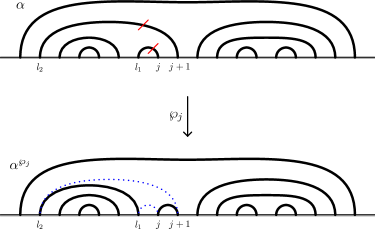
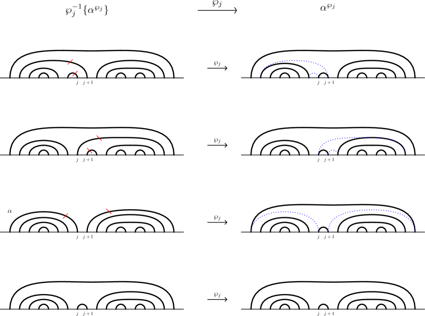
The solutions $(v_{\alpha})_{\alpha\in\mathrm{LP}}$ will be shown to have a certain property, which is also used for their construction recursively down the partially ordered set of link patterns (see Figure 3.2). A closely related formula for connectivity weights was independently observed in [FK15d, Equation (69)]. This key property is the equality

(3.10) $$v_{\alpha}=\left[2\right]\,\Big{(}\mathrm{id}-\pi_{j}\Big{)}\,(v_{\alpha^{\wp_{j}}})\;-\;\sum_{\begin{subarray}{c}\beta\in\mathrm{LP}_{N}\setminus\{\alpha,\alpha^{\wp_{j}}\}\\ \beta^{\wp_{j}}\,=\,\alpha^{\wp_{j}}\end{subarray}}\;v_{\beta}$$

whenever $\alpha\in\mathrm{LP}_{N}$ and $j$ is such that $[\wideparen{l_{1},j}],[\wideparen{j+1,l_{2}}]\in\alpha$ with $l_{1}<j<j+1<l_{2}$. Before turning to the construction, we record some combinatorial observations about this setup.

Lemma 3.5.

Fix $\alpha\in\mathrm{LP}_{N}$. The following are equivalent for $j\in\left\{1,\ldots,2N-1\right\}$:

(i):

$[\wideparen{l_{1},j}],[\wideparen{j+1,l_{2}}]\in\alpha$ with $l_{1}<j<j+1<l_{2}$.

(ii):

$[\wideparen{j,j+1}]\notin\alpha$, and $\alpha\preceq\beta$ for all $\beta\in\wp_{j}^{-1}\left\{\alpha^{\wp_{j}}\right\}$.

Moreover, an index $j$ satisfying (i) and (ii) exists if $\alpha\neq\boldsymbol{\underline{\Cap}}_{N}$, and the following properties then hold.

(a):

If $|k-j|=1$, then there exists a unique $\beta_{0}\in\wp_{j}^{-1}\left\{\alpha^{\wp_{j}}\right\}$ such that $[\wideparen{k,k+1}]\in\beta_{0}$. This $\beta_{0}$ satisfies $\beta_{0}/[\wideparen{k,k+1}]=\alpha^{\wp_{j}}/[\wideparen{j,j+1}]$.

(b):

If $|k-j|>1$ and $[\wideparen{k,k+1}]\notin\alpha$, then $[\wideparen{k,k+1}]\notin\alpha^{\wp_{j}}$.

(c):

If $|k-j|>1$ and $[\wideparen{k,k+1}]\in\alpha$, then the mapping $\beta\mapsto\hat{\beta}=\beta/[\wideparen{k,k+1}]$ defines a bijection

$$\Big{\{}\beta\in\wp_{j}^{-1}\left\{\alpha^{\wp_{j}}\right\}\;\Big{|}\;[\wideparen{k,k+1}]\in\beta\Big{\}}\;\longrightarrow\;\wp_{j^{\prime}}^{-1}\left\{\hat{\alpha}^{\wp_{j^{\prime}}}\right\},$$

where $\hat{\alpha}=\alpha/[\wideparen{k,k+1}]$, and $j^{\prime}=j$ if $k>j$ and $j^{\prime}=j-2$ if $k<j$.

Proof.

The equivalence of (i) and (ii) is straightforward from the definition of the partial order. See also Figure 3.4.

For $\alpha\neq\boldsymbol{\underline{\Cap}}_{N}$, the existence of $j$ satisfying condition (i) is easy to see. For property (a), the desired link pattern is $\beta_{0}=(\alpha^{\wp_{j}})^{\wp_{k}}$ — this is illustrated in Figure 3.5. Property (b) follows from (i). For property (c), the assumption of the presence of the link $[\wideparen{k,k+1}]$ implies that neither $j$ nor $j+1$ is connected to $k$ or $k+1$, so the link $[\wideparen{k,k+1}]$ plays no role in the tying operations: the map is well defined to the asserted range, and the inverse map is obvious. ∎

Figure 3.5. Suppose $k=j-1$ and $j$ is chosen as in Lemma 3.5(i). The unique $\beta_{0}\in\wp_{j}^{-1}\left\{\alpha^{\wp_{j}}\right\}$ containing the link $[\wideparen{k,k+1}]=[\wideparen{k,j}]$ can be found by applying the map $\wp_{k}$ to the link pattern $\alpha^{\wp_{j}}$, as depicted in the figure. Notice also that we clearly have $\beta_{0}/[\wideparen{k,k+1}]=\alpha^{\wp_{j}}/[\wideparen{j,j+1}]$.

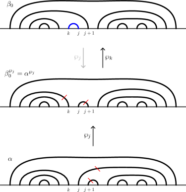
We are now ready to construct the solutions to (3.1) – (3.3) for all $\alpha\in\mathrm{LP}$ from the solutions corresponding to the maximal patterns $\boldsymbol{\underline{\Cap}}_{N}$, given in Proposition 3.3.

Proposition 3.6.

Let $\alpha\in\mathrm{LP}_{N}\setminus\{\boldsymbol{\underline{\Cap}}_{N}\}$. Suppose that the collection $\left(v_{\beta}\right)_{\beta\in\mathrm{LP}^{\succ\alpha}}$ satisfies the system (3.1) – (3.3) and the equations (3.10) for all $\beta\in\mathrm{LP}^{\succ\alpha}$. Then the vector $v_{\alpha}\in\mathsf{M}_{2}^{\otimes 2N}$ can be defined in accordance with Equation (3.10) as

$$v_{\alpha}\;:=\;\left[2\right]\,\Big{(}\mathrm{id}-\pi_{j}\Big{)}\,(v_{\alpha^{\wp_{j}}})\;-\;\sum_{\begin{subarray}{c}\beta\in\mathrm{LP}_{N}\setminus\{\alpha,\alpha^{\wp_{j}}\}\\ \beta^{\wp_{j}}\,=\,\alpha^{\wp_{j}}\end{subarray}}\;v_{\beta}$$

for any $j$ as in Lemma 3.5. This vector is a solution to (3.1) – (3.3) for $\alpha$.

Proof.

Choose a $j$ as in Lemma 3.5. By property (ii), the link patterns $\alpha^{\wp_{j}}$ and $\beta$ needed in the formula defining $v_{\alpha}$ satisfy $\alpha^{\wp_{j}}\succ\alpha$ and $\beta\succ\alpha$, and the corresponding vectors $v_{\alpha^{\wp_{j}}}$ and $v_{\beta}$ are thus assumed given. By assumption, each of these vectors satisfies (3.1) – (3.3), so it readily follows that $v_{\alpha}$ also satisfies (3.1) and (3.2). It remains to be shown that for any $k\in\{1,\ldots,2N-1\}$, the projection $\hat{\pi}_{k}(v_{\alpha})$ gives (3.3). Note that once we have shown that $v_{\alpha}$ satisfies (3.1) – (3.3), it follows from the uniqueness argument of Proposition 3.2 that the constructed vector $v_{\alpha}$ is independent of the choice of $j$, and thus in particular satisfies (3.10).

We divide the calculations to three separate cases: (i): $k=j$, (ii): $\,|k-j|=1\,$ and (iii): $\,|k-j|>1$.

Let us start from the easiest case (i): $k=j$. To establish (3.3) in this case, we need to show $\hat{\pi}_{j}(v_{\alpha})=0$. Since $\pi_{j}$ is a projection, the first term $(\mathrm{id}-\pi_{j})\,(v_{\alpha^{\wp_{j}}})$ in the formula defining $v_{\alpha}$ is annihilated by $\hat{\pi}_{j}$. We have $\hat{\pi}_{j}(v_{\beta})=0$ also for all the other terms, since $[\wideparen{j,j+1}]\notin\beta$ for $\beta\in\big{(}\wp_{j}^{-1}\left\{\alpha\right\}\big{)}\setminus\{\alpha,\alpha^{\wp_{j}}\}$. This concludes the case (i).

Consider then the case (ii): $\,|k-j|=1$. We need to compute $\hat{\pi}_{k}(v_{\alpha})$ and compare with (3.3). The application of $\pi_{k}$ on the first term of the formula defining $v_{\alpha}$ gives

$$\left[2\right]\,\pi_{k}\Big{(}\mathrm{id}-\pi_{j}\Big{)}(v_{\alpha^{\wp_{j}}})\;=\;-\left[2\right]\,\Big{(}\pi_{k}\circ\pi_{j}\Big{)}(v_{\alpha^{\wp_{j}}})$$

since $[\wideparen{k,k+1}]\notin\alpha^{\wp_{j}}$. Now, (3.3) for $\alpha^{\wp_{j}}$ gives $\hat{\pi}_{j}(v_{\alpha^{\wp_{j}}})=v_{\alpha^{\wp_{j}}/[\wideparen{j,j+1}]}$ and we see that the vector $\pi_{j}(v_{\alpha^{\wp_{j}}})$ can be obtained from $v_{\alpha^{\wp_{j}}/[\wideparen{j,j+1}]}\in\mathsf{M}_{2}^{\otimes 2(N-1)}$ by inserting the singlet vector $s\in\mathsf{M}_{2}\otimes\mathsf{M}_{2}$ into the $j$:th and $j+1$:st tensor positions. Therefore, by Lemma 2.3(b), we obtain

$$\left[2\right]\,\hat{\pi}_{k}\Big{(}\mathrm{id}-\pi_{j}\Big{)}(v_{\alpha^{\wp_{j}}})\;=\;-\left[2\right]\,\Big{(}\hat{\pi}_{k}\circ\pi_{j}\Big{)}(v_{\alpha^{\wp_{j}}})\;=\;v_{\alpha^{\wp_{j}}/[\wideparen{j,j+1}]}.$$

In the sum in the formula defining $v_{\alpha}$, only the term corresponding to the link pattern $\beta_{0}$ of Lemma 3.5(a) can survive the projection $\pi_{k}$, as the others do not contain the link $[\wideparen{k,k+1}]$. Therefore,

$$\hat{\pi}_{k}\Big{(}\sum_{\begin{subarray}{c}\beta\in\mathrm{LP}_{N}\setminus\{\alpha,\alpha^{\wp_{j}}\}\\ \beta^{\wp_{j}}\,=\,\alpha^{\wp_{j}}\end{subarray}}\;v_{\beta}\Big{)}\;=\; \begin{cases}\hat{\pi}_{k}(v_{\beta_{0}})\;=\;v_{\beta_{0}/[\wideparen{k,k+1}]}&\text{if }\beta_{0}\neq\alpha\\ 0\qquad&\text{if }\beta_{0}=\alpha.\end{cases}$$

The patterns $\beta_{0}/[\wideparen{k,k+1}]$ and $\alpha^{\wp_{j}}/[\wideparen{j,j+1}]$ are the same by Lemma 3.5(a), and $[\wideparen{k,k+1}]\in\alpha$ if and only if $\beta_{0}=\alpha$. We can therefore combine the above observations and conclude that

$$\hat{\pi}_{k}(v_{\alpha})=\begin{cases}v_{\alpha^{\wp_{j}}/[\wideparen{j,j+1}]}\,-\,v_{\beta_{0}/[\wideparen{k,k+1}]}\;=\;0&\text{if }\beta_{0}\neq\alpha\\ v_{\alpha^{\wp_{j}}/[\wideparen{j,j+1}]}\qquad\qquad\qquad\;=\;v_{\alpha/[\wideparen{k,k+1}]}\qquad&\text{if }\beta_{0}=\alpha.\end{cases}$$

This shows (3.3) for $\alpha$, and concludes the case (ii).

Finally, consider the case (iii): $\,|k-j|>1$. We must again calculate $\hat{\pi}_{k}(v_{\alpha})$. The projections $\pi_{j}$ and $\pi_{k}$ now commute, and thus the projection $\pi_{k}$ of the first term in the defining equation of $v_{\alpha}$ reads

(3.11) $$\left[2\right]\,\pi_{k}\Big{(}\mathrm{id}-\pi_{j}\Big{)}(v_{\alpha^{\wp_{j}}})\;=\;\left[2\right]\,\Big{(}\mathrm{id}-\pi_{j}\Big{)}\pi_{k}(v_{\alpha^{\wp_{j}}})$$

and the projection $\hat{\pi}_{k}$ of the second term reads

(3.12) $$\hat{\pi}_{k}\Big{(}\sum_{\begin{subarray}{c}\beta\in\mathrm{LP}_{N}\setminus\{\alpha,\alpha^{\wp_{j}}\}\\ \beta^{\wp_{j}}\,=\,\alpha^{\wp_{j}}\end{subarray}}\;v_{\beta}\Big{)}\;=\;\sum_{\begin{subarray}{c}\beta\in\mathrm{LP}_{N}\setminus\{\alpha,\alpha^{\wp_{j}}\}\\ \beta^{\wp_{j}}\,=\,\alpha^{\wp_{j}},\;[\wideparen{k,k+1}]\in\beta\end{subarray}}\;v_{\beta/[\wideparen{k,k+1}]}.$$

Suppose first that $[\wideparen{k,k+1}]\notin\alpha$, in which case we need to show $\hat{\pi}_{k}(v_{\alpha})=0$. By Lemma 3.5(b), in this case also $[\wideparen{k,k+1}]\notin\alpha^{\wp_{j}}$, so $\hat{\pi}_{k}(v_{\alpha^{\wp_{j}}})=0$ and (3.11) is zero. Also (3.12) is zero because the sum on the right hand side of (3.12) is empty. Thus we indeed have $\hat{\pi}_{k}(v_{\alpha})=0$.

Suppose then that $[\wideparen{k,k+1}]\in\alpha$, in which case we need to show $\hat{\pi}_{k}(v_{\alpha})=v_{\alpha/[\wideparen{k,k+1}]}$. Using the bijection $\beta\mapsto\hat{\beta}:=\beta/[\wideparen{k,k+1}]$ of Lemma 3.5(c), we rewrite the summation in (3.12) as

$$\hat{\pi}_{k}\Big{(}\sum_{\begin{subarray}{c}\beta\in\mathrm{LP}_{N}\setminus\{\alpha,\alpha^{\wp_{j}}\}\\ \beta^{\wp_{j}}\,=\,\alpha^{\wp_{j}}\end{subarray}}\;v_{\beta}\Big{)}\;=\;\sum_{\begin{subarray}{c}\beta\in\mathrm{LP}_{N}\setminus\{\alpha,\alpha^{\wp_{j}}\}\\ \beta^{\wp_{j}}\,=\,\alpha^{\wp_{j}},\;[\wideparen{k,k+1}]\in\beta\end{subarray}}\;v_{\beta/[\wideparen{k,k+1}]}\,=\,\sum_{\begin{subarray}{c}\hat{\beta}\in\mathrm{LP}_{N-1}\setminus\{\hat{\alpha},\hat{\alpha}^{\wp_{j^{\prime}}}\}\\ \hat{\beta}^{\wp_{j^{\prime}}}\,=\,\hat{\alpha}^{\wp_{j^{\prime}}}\end{subarray}}\;v_{\hat{\beta}}.$$

In (3.11), we use $\hat{\pi}_{k}(v_{\alpha^{\wp_{j}}})=v_{\hat{\alpha}^{\wp_{j^{\prime}}}}$, and combine to obtain

$$\hat{\pi}_{k}(v_{\alpha})= \;\left[2\right]\,\Big{(}\mathrm{id}-\pi_{j^{\prime}}\Big{)}\,(v_{\hat{\alpha}^{\wp_{j^{\prime}}}})\;-\;\sum_{\begin{subarray}{c}\hat{\beta}\in\mathrm{LP}_{N-1}\setminus\{\hat{\alpha},\hat{\alpha}^{\wp_{j^{\prime}}}\}\\ \hat{\beta}^{\wp_{j^{\prime}}}\,=\,\hat{\alpha}^{\wp_{j^{\prime}}}\end{subarray}}\;v_{\hat{\beta}}.$$

By the assumed equality (3.10), this expression is $v_{\hat{\alpha}}$, which is what we wanted to show. This concludes the case (iii) and completes the proof. ∎

3.4. Proof of Theorem 3.1

Uniqueness follows immediately from Proposition 3.2. Proposition 3.3 gives the solution $v_{\boldsymbol{\underline{\Cap}}_{N}}$ for each $N\in\mathbb{Z}_{\geq 0}$. From this solution, corresponding to the maximal element $\boldsymbol{\underline{\Cap}}_{N}$ of the partially ordered set $\mathrm{LP}_{N}$, Proposition 3.6 allows us to construct the solutions $v_{\alpha}$ for $\alpha\in\mathrm{LP}_{N}\setminus\{\boldsymbol{\underline{\Cap}}_{N}\}$ recursively in any order that refines the partial order. $\hfill\qed$

3.5. Basis of the trivial subrepresentation

In this section, consider a fixed $N\in\mathbb{N}$. The trivial subrepresentation $\mathsf{H}_{1}=\mathsf{H}_{1}(\mathsf{M}_{2}^{\otimes 2N})$, introduced in (2.7), is exactly the solution space of (3.1) – (3.2). The vectors $v_{\alpha}$ satisfying the projection conditions (3.3) for $\alpha\in\mathrm{LP}_{N}$ in fact constitute a basis of this subspace, as we will show below in Proposition 3.7(b). For this purpose, we define certain elements $\psi_{\alpha}$ of the dual space $\mathsf{H}_{1}^{*}=\left\{\psi\colon\mathsf{H}_{1}\to\mathbb{C}\;|\;\psi\text{ is a linear map}\right\}$, which will be shown to form the dual basis of $(v_{\alpha})_{\alpha\in\mathrm{LP}_{N}}$. The definition and construction are analogous to those of a dual basis of the solution space of (1.2) – (1.3) in [FK15a], and we follow some similar terminology and notation.

Consider the link pattern

$$\alpha=\left\{[\wideparen{a_{1},b_{1}}],\ldots,[\wideparen{a_{N},b_{N}}]\right\}\in\mathrm{LP}_{N}$$

together with an ordering of the links: $[\wideparen{a_{1},b_{1}}],\ldots,[\wideparen{a_{N},b_{N}}]$. We use the convention that $a_{j}<b_{j}$ for all $j=1,\ldots,N$, i.e., $a_{j}$ is the index of the left endpoint of the $j$:th link. One possible choice of ordering is by the left endpoints of the links — the ordering $[\wideparen{a^{\circ}_{1},b^{\circ}_{1}}],\ldots,[\wideparen{a^{\circ}_{N},b^{\circ}_{N}}]$ such that $a^{\circ}_{1}<a^{\circ}_{2}<\cdots<a^{\circ}_{N}$ will be used as a reference to which other choices of orderings are compared: for some permutation $\sigma\in\mathfrak{S}_{N}$ we have $a_{j}=a^{\circ}_{\sigma(j)}$, $b_{j}=b^{\circ}_{\sigma(j)}$ for all $j=1,\ldots,N$.

If $a_{1},b_{1}$ are consecutive indices, $b_{1}=a_{1}+1$, then $\alpha/[\wideparen{a_{1},b_{1}}]$ denotes the link pattern with the first link removed. The indices of the other $N-1$ links $[\wideparen{a_{2},b_{2}}]$, …, $[\wideparen{a_{N},b_{N}}]$ are relabeled, so that the links of $\alpha/[\wideparen{a_{1},b_{1}}]$ are $[\wideparen{a_{2}(1),b_{2}(1)}]$, …, $[\wideparen{a_{N}(1),b_{N}(1)}]$, respectively. Iteratively, if $a_{j}(j-1),b_{j}(j-1)$ are consecutive after removal of $j-1$ first links, i.e., $b_{j}(j-1)=a_{j}(j-1)+1$, then the $j$:th link can be removed to obtain a link pattern denoted by $\alpha/[\wideparen{a_{1},b_{1}}]/\cdots/[\wideparen{a_{j},b_{j}}]$. With relabeling the indices, as in Figure 3.6, the remaining $N-j$ links are denoted by $[\wideparen{a_{j+1}(j),b_{j+1}(j)}]$, …, $[\wideparen{a_{N}(j),b_{N}(j)}]$. The ordering $\sigma$ is said to be allowable for $\alpha$ if all links of $\alpha$ can be removed in the order $\sigma$, i.e., if we have $b_{j+1}(j)=a_{j+1}(j)+1$ for all $j<N$.

Figure 3.6. The ordering $\left\{[\wideparen{3,4}],[\wideparen{2,5}],[\wideparen{6,7}],[\wideparen{1,8}],[\wideparen{11,12}],[\wideparen{10,13}],[\wideparen{9,14}]\right\}$ is allowable for $\alpha$ as depicted in the figure. The figure also illustrates the iterated projections appearing in the definition of the map $\psi_{\alpha}$ in (3.13), with relabeled indices.

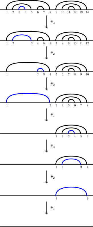
Let $\alpha\in\mathrm{LP}_{N}$ and let $\sigma\in\mathfrak{S}_{N}$ be an allowable ordering for $\alpha$. We define the linear map

(3.13) $$\psi_{\alpha}^{(\sigma)}\colon \mathsf{H}_{1}\longrightarrow\mathbb{C},\qquad\psi_{\alpha}^{(\sigma)}:=\;\hat{\pi}_{a_{N}(N-1)}\circ\cdots\circ\hat{\pi}_{a_{2}(1)}\circ\hat{\pi}_{a_{1}},$$

where $\hat{\pi}_{a_{j}(j-1)}\colon\mathsf{M}_{2}^{\otimes 2(N-j+1)}\to\mathsf{M}_{2}^{\otimes 2(N-j)}$ are projections in the tensor components $a_{j}(j-1)$ and $a_{j}(j-1)+1=b_{j}(j-1)$, reducing the number of tensorands by two — see Figure 3.6.

We next show that $\psi_{\alpha}^{(\sigma)}$ is in fact independent of the choice of allowable ordering $\sigma$ for $\alpha$, and thus gives rise to a well defined linear map

(3.14) $$\psi_{\alpha}:=\psi_{\alpha}^{(\sigma)}\;\colon\;\mathsf{H}_{1}\longrightarrow\mathbb{C}$$

for any choice of allowable $\sigma=\sigma(\alpha)\in\mathfrak{S}_{N}$, and that $\left(\psi_{\alpha}\right)_{\alpha\in\mathrm{LP}_{N}}$ is a basis of the dual space $\mathsf{H}_{1}^{*}$.

Proposition 3.7.

(a):

Let $\alpha\in\mathrm{LP}_{N}$. For any two allowable orderings $\sigma,\sigma^{\prime}\in\mathfrak{S}_{N}$ for $\alpha$, we have

$$\psi_{\alpha}^{(\sigma)}=\psi_{\alpha}^{(\sigma^{\prime})}.$$

Thus, the linear functional $\psi_{\alpha}\in\mathsf{H}_{1}^{*}$ in (3.14) is well defined.

(b):

For any $\alpha,\beta\in\mathrm{LP}_{N}$ we have

(3.15) $$\psi_{\alpha}(v_{\beta})\;=\;\delta_{\alpha,\beta}\;=\; \begin{cases}1\quad&\text{if }\beta=\alpha\\ 0&\text{if }\beta\neq\alpha\end{cases}.$$

In particular, $\left(v_{\alpha}\right)_{\alpha\in\mathrm{LP}_{N}}$ and $\left(\psi_{\alpha}\right)_{\alpha\in\mathrm{LP}_{N}}$ are bases of $\mathsf{H}_{1}$ and $\mathsf{H}_{1}^{*}$, respectively, and dual to each other.

Proof.

Let $\alpha,\beta\in\mathrm{LP}_{N}$, and let $\sigma\in\mathfrak{S}_{N}$ be any allowable ordering for $\alpha$. Consider $\psi_{\alpha}^{(\sigma)}(v_{\beta})$. If $\beta=\alpha$, then by (3.3) we have $\hat{\pi}_{a_{1}}(v_{\alpha})=v_{\alpha/[\wideparen{a_{1},b_{1}}]}$, and recursively,

$$\Big{(}\hat{\pi}_{a_{j}(j-1)}\circ\cdots\circ\hat{\pi}_{a_{1}}\Big{)}(v_{\alpha})=v_{\alpha/[\wideparen{a_{1},b_{1}}]/\cdots/[\wideparen{a_{j},b_{j}}]}.$$

For $j=N$ this gives $\psi_{\alpha}^{(\sigma)}(v_{\alpha})=v_{\emptyset}=1$. On the other hand, if $\beta\neq\alpha$, then for some $j$ we have $[\wideparen{a_{j},b_{j}}]\notin\beta$, and by (3.3) we then similarly get $\psi_{\alpha}^{(\sigma)}(v_{\beta})=0$. Summarizing, Equation (3.15) holds: we have $\psi_{\alpha}^{(\sigma)}(v_{\beta})=\delta_{\alpha,\beta}$, independently of the choice of allowable $\sigma$. In particular, the value of the operator $\psi_{\alpha}^{(\sigma)}$ in the linear span of the vectors $v_{\beta}$ is independent of the choice of allowable $\sigma$. Assertion (a) will follow by showing that this linear span is actually the whole space $\mathsf{H}_{1}$.

In the linear span of the vectors $v_{\beta}$, we now set $\psi_{\alpha}:=\psi_{\alpha}^{(\sigma)}$. The collection $\left(\psi_{\alpha}\right)_{\alpha\in\mathrm{LP}_{N}}$ of linear functionals on $\mathrm{span}\{v_{\beta}\;|\;\beta\in\mathrm{LP}_{N}\}$ is linearly independent — indeed, any linear relation

$$\psi_{\beta}=\sum_{\alpha\in\mathrm{LP}_{N}\setminus\{\beta\}}c_{\alpha}\psi_{\alpha}$$

would by (3.15) lead to a contradiction

$$1=\psi_{\beta}(v_{\beta})=\sum_{\alpha\in\mathrm{LP}_{N}\setminus\{\beta\}}c_{\alpha}\,\psi_{\alpha}(v_{\beta})=\sum_{\alpha\in\mathrm{LP}_{N}\setminus\{\beta\}}c_{\alpha}\delta_{\alpha,\beta}=0.$$

Since we have $\mathrm{dim}(\mathsf{H}_{1})=\mathrm{dim}(\mathsf{H}_{1}^{*})=\mathrm{C}_{N}=\#\mathrm{LP}_{N}$ by Lemma 2.2, it follows that $\left(\psi_{\alpha}\right)_{\alpha\in\mathrm{LP}_{N}}$ is a basis of the whole dual space $\mathsf{H}_{1}^{*}$, and $\left(v_{\alpha}\right)_{\alpha\in\mathrm{LP}_{N}}$ its dual basis in $\mathsf{H}_{1}$. This concludes the proof. ∎

4. Multiple $\mathrm{SLE}$ partition functions

In this section, we consider multiple $\mathrm{SLE}$ partition functions constructed from the vectors $v_{\alpha}$ of Section 3, using the correspondence of Theorem 2.6. We give in Section 4.1 the construction and properties of the pure partition functions $\mathcal{Z}_{\alpha}$, i.e., solutions to the system (1.2) – (1.4). Section 4.2 contains the only remaining part of the proof of the properties, namely the injectivity of the correspondence of Theorem 2.6. In Section 4.3, we consider partition functions $\mathcal{Z}^{(N)}$ that are most commonly relevant for statistical physics models — these symmetric partition functions are combinations of the pure partition functions. Finally, Sections 4.4 – 4.6 give examples of symmetric partition functions applicable to a few important lattice models. These are explicit solutions to the partial differential equations at particular values of $\kappa$, and as such, they are relevant to the construction of local multiple $\mathrm{SLE}$s by the results of Appendix A. These values of $\kappa$ are rational, and therefore the solutions are not strictly speaking special cases of our generic solutions for $\kappa\in(0,8)\setminus\mathbb{Q}$, but should be obtained via a suitable limiting procedure.

4.1. Pure partition functions

In this section, we will use the mappings

$$\mathcal{F}\colon\mathsf{H}_{1}(\mathsf{M}_{2}^{\otimes 2N})\to\mathcal{C}^{\infty}(\mathfrak{X}_{2N})$$

given by Theorem 2.6, to construct the pure partition functions $(\mathcal{Z}_{\alpha})_{\alpha\in\mathrm{LP}}$ from the vectors $(v_{\alpha})_{\alpha\in\mathrm{LP}}$ of Theorem 3.1. Recall from Theorem 2.6 the following important properties for any vector $v$ in the trivial subrepresentation $\mathsf{H}_{1}=\mathsf{H}_{1}(\mathsf{M}_{2}^{\otimes 2N})$:

• (PDE) ensures that the function $\mathcal{F}[v]$ is a solution to the PDEs (1.2).

• (COV) gives the Möbius covariance (1.3).

• (ASY) enables us to pick solutions of (1.2) – (1.3) with the desired asymptotic properties (1.4).

We will show in Corollary 4.3 that, for all $N\in\mathbb{N}$, the map $\mathcal{F}$ is injective and thus the basis $\left(v_{\alpha}\right)_{\alpha\in\mathrm{LP}_{N}}$ of $\mathsf{H}_{1}$ given by Proposition 3.7(b) provides a basis for the solution space $\mathcal{F}[\mathsf{H}_{1}]=\mathcal{F}[\mathsf{H}_{1}(\mathsf{M}_{2}^{\otimes 2N})]$ of the system (1.2) – (1.3). We normalize this basis by $B^{-|\alpha|}\,\mathcal{F}[v_{\alpha}]$, where $B=\frac{\Gamma(1-4/\kappa)^{2}}{\Gamma(2-8/\kappa)}$ — this choice of normalization is convenient by the (ASY) part of Theorem 2.6. Notice that with our assumption $\kappa\notin\mathbb{Q}$, the normalizing constant $B^{-|\alpha|}$ is finite and non-zero.

Theorem 4.1.

Let $\kappa\in(0,8)\setminus\mathbb{Q}$. The collection $\left(\mathcal{Z}_{\alpha}\right)_{\alpha\in\mathrm{LP}}$ of functions

$$\mathcal{Z}_{\alpha}:=B^{-|\alpha|}\,\mathcal{F}[v_{\alpha}]\;\colon\;\mathfrak{X}_{2|\alpha|}\rightarrow\mathbb{C}$$

satisfies the system of equations (1.2) – (1.4) for all $\alpha\in\mathrm{LP}$. For any $N\in\mathbb{Z}_{\geq 0}$, the collection $\left(\mathcal{Z}_{\alpha}\right)_{\alpha\in\mathrm{LP}_{N}}$ is linearly independent and it spans the $\mathrm{C}_{N}$-dimensional space $\mathcal{F}[\mathsf{H}_{1}(\mathsf{M}_{2}^{\otimes 2N})]$ of solutions to the system (1.2) – (1.3).

Proof.

By Theorem 2.6, since the vectors $v_{\alpha}$ satisfy (3.1) – (3.2), the functions $\mathcal{Z}_{\alpha}=B^{-|\alpha|}\mathcal{F}[v_{\alpha}]$ satisfy (1.2) – (1.3). The asymptotic conditions (1.4) follow from the (ASY) part of Theorem 2.6, by the projection conditions (3.3) for the vectors $v_{\alpha}$. The final assertion of linear independence will be established in Proposition 4.2 in the next section. ∎

4.2. Linear independence of the pure partition functions

To show that $\left(\mathcal{Z}_{\alpha}\right)_{\alpha\in\mathrm{LP}_{N}}$ is a basis of the $\mathrm{C}_{N}$-dimensional solution space $\mathcal{F}[\mathsf{H}_{1}]$, we use linear mappings $\mathscr{L}_{\alpha}$, closely related to the maps $\psi_{\alpha}$ from (3.14), defined by iterated limits. We show in Proposition 4.2 that $\left(\mathscr{L}_{\alpha}\right)_{\alpha\in\mathrm{LP}_{N}}$ is a basis of the dual space $\mathcal{F}[\mathsf{H}_{1}]^{*}$ and that the functions $\mathcal{Z}_{\alpha}=B^{-|\alpha|}\,\mathcal{F}[v_{\alpha}]$ constitute its dual basis. These iterated limits were originally introduced in [FK15a], where their well-definedness was checked with analysis techniques. With the quantum group method of [KP14] and the solutions $(v_{\alpha})_{\alpha\in\mathrm{LP}_{N}}$, the well-definedness on the $\mathrm{C}_{N}$-dimensional solution space $\mathcal{F}[\mathsf{H}_{1}]$ becomes almost immediate.

Suppose the ordering $\sigma\in\mathfrak{S}_{N}$ is allowable for $\alpha\in\mathrm{LP}_{N}$, and let $[\wideparen{a_{1},b_{1}}],\ldots,[\wideparen{a_{N},b_{N}}]$ be the corresponding links (recall Section 3.5 and Figure 3.6). By the (ASY) part of Theorem 2.6, the following sequence of limits exists for any $\mathcal{Z}=\mathcal{F}[v]\in\mathcal{F}[\mathsf{H}_{1}]$:

(4.1) $$\mathscr{L}_{\alpha}^{(\sigma)}(\mathcal{Z}):=\;\lim_{x_{a_{N}},x_{b_{N}}\to\xi_{N}}\cdots\lim_{x_{a_{1}},x_{b_{1}}\to\xi_{1}}(x_{b_{N}}-x_{a_{N}})^{2h}\cdots(x_{b_{1}}-x_{a_{1}})^{2h}\times\mathcal{Z}(x_{1},\ldots,x_{2N}).$$

Note that each of the limits in (4.1) is independent of the limit point $\xi_{j}$, and (4.1) in fact equals $B^{|\alpha|}\psi_{\alpha}(v)$, where $\psi_{\alpha}\colon\mathsf{H}_{1}\longrightarrow\mathbb{C}$ is the linear map introduced in (3.14). In particular, the linear map

$$\mathscr{L}_{\alpha}:=\mathscr{L}_{\alpha}^{(\sigma)}\;\colon\;\mathcal{F}[\mathsf{H}_{1}]\rightarrow\mathbb{C}$$

is well defined via Equation (4.1), independently of the choice of allowable ordering $\sigma$ for $\alpha$.

Proposition 4.2.

The collection $\left(\mathscr{L}_{\alpha}\right)_{\alpha\in\mathrm{LP}_{N}}$ is a basis of the dual space $\mathcal{F}[\mathsf{H}_{1}]^{*}$, and we have

$$\mathscr{L}_{\alpha}(\mathcal{Z}_{\beta})\;=\;\delta_{\alpha,\beta}\;=\; \begin{cases}1\quad&\text{if }\beta=\alpha\\ 0&\text{if }\beta\neq\alpha\end{cases}.$$

In particular, $\left(\mathcal{Z}_{\alpha}\right)_{\alpha\in\mathrm{LP}_{N}}$ is a basis of the $\mathrm{C}_{N}$-dimensional solution space $\mathcal{F}[\mathsf{H}_{1}]$.

In [FK15d], “connectivity weights” are defined as the dual basis of the iterated limits $\mathscr{L}_{\alpha}$, so by this proposition they coincide with our pure partition functions. Explicit expressions for the connectivity weights for $N=2,3,4$ were studied further in [FSK15], and a formula [FSK15, Equation (56)] for the connectivity weight of the rainbow pattern (see Proposition 3.3) was obtained for general $N$.

Proof of Proposition 4.2.

The assertion follows directly from Proposition 3.7, because we have $\mathcal{Z}_{\alpha}=B^{-|\alpha|}\,\mathcal{F}[v_{\alpha}]$ by definition, and hence, $\mathscr{L}_{\alpha}(\mathcal{Z}_{\beta})=B^{|\alpha|}\,\psi_{\alpha}(B^{-|\beta|}v_{\beta})=\delta_{\alpha,\beta}$. ∎

As a corollary, we get the injectivity of the “spin chain – Coulomb gas correspondence” $\mathcal{F}$.

Corollary 4.3.

For any $N\in\mathbb{Z}_{>0}$, the mapping $\mathcal{F}\colon\mathsf{H}_{1}(\mathsf{M}_{2}^{\otimes 2N})\rightarrow\mathcal{C}^{\infty}(\mathfrak{X}_{2N})$ is injective.

Proof.

By Proposition 4.2, the images $\mathcal{F}[v_{\alpha}]$ of the basis vectors $v_{\alpha}$ of $\mathsf{H}_{1}(\mathsf{M}_{2}^{\otimes 2N})$ are linearly independent, because $\mathcal{Z}_{\alpha}=B^{-|\alpha|}\,\mathcal{F}[v_{\alpha}]$ are. Injectivity of $\mathcal{F}$ follows by linearity. ∎

4.3. Symmetric partition functions and entire curve domain Markov property

In this section, we study partition functions relevant for statistical mechanics models admitting a cyclic permutation symmetry of the marked points on the boundary. Examples of such models are critical percolation, the Ising model at criticality, and the discrete Gaussian free field, with suitable boundary conditions.

The symmetric partition functions $\mathcal{Z}^{(N)}$ are combinations of the extremal, pure partition functions $\mathcal{Z}_{\alpha}$, and this combination encodes information about the crossing probabilities of the model. Formulas for $\mathcal{Z}^{(N)}$ are in fact often easier to find than those for $\mathcal{Z}_{\alpha}$. Explicit formulas for crossing probabilities, however, require the knowledge of the pure partition functions as well.

The functions $\mathcal{Z}^{(N)}$ should satisfy the conditions of Theorem A.4(a), in particular, Equations (1.2) and (1.3). The asymptotics requirement (1.4) is replaced by the cascade property

(4.2) $$\lim_{x_{j},x_{j+1}\to\xi}\frac{\mathcal{Z}^{(N)}(x_{1},\ldots,x_{2N})}{(x_{j+1}-x_{j})^{-2h}}=\; \mathcal{Z}^{(N-1)}(x_{1},\ldots,x_{j-1},x_{j+2},\ldots,x_{2N})$$

for any $j=1,\ldots,2N-1$. This expresses the fact that the partition function of the model with $2N$ boundary changes reduces to that with $2N-2$ boundary changes as any two marked points are merged. In view of Proposition A.6, in this limit the other curves do not feel the merged marked points, and they have the law of the symmetric $(N-1)$-$\mathrm{SLE}$. Roughly, this should be interpreted as a domain Markov property with respect to one entire curve of the multiple $\mathrm{SLE}$.

By our correspondence, Theorem 2.6, such symmetric partition functions $\mathcal{Z}^{(N)}$ can be constructed as $\mathcal{Z}^{(N)}\propto\mathcal{F}[v^{(N)}]$ from vectors $v^{(N)}\in\mathsf{M}_{2}^{\otimes 2N}$ satisfying the following system of equations:

(4.3) $$K.v^{(N)}=v^{(N)}$$

(4.4) $$E.v^{(N)}=0$$

(4.5) $$\hat{\pi}_{j}(v^{(N)})=v^{(N-1)}\qquad\text{for all}\;j=1,\ldots,2N-1.$$

In the quantum group setting, we have a unique solution for this system when the normalization is fixed.

Theorem 4.4.

There exists a unique collection $\left(v^{(N)}\right)_{N\in\mathbb{Z}_{\geq 0}}$ of vectors in $\mathsf{M}_{2}^{\otimes 2N}$ such that $v^{(0)}=1$ and the system of equations (4.3) – (4.5) hold for all $N\in\mathbb{Z}_{>0}$. The vectors are given by

$$v^{(N)}=\sum_{\alpha\in\mathrm{LP}_{N}}v_{\alpha}.$$

Proof.

Applying Corollary 2.5 to the difference of two solutions gives uniqueness, as in the proof of Proposition 3.2. It remains to check that the asserted formula satisfies (4.3) – (4.5). Equations (4.3) – (4.4) are satisfied by (3.1) – (3.2). For (4.5), we use the properties (3.3) of the vectors $v_{\alpha}$, and the bijection $\left\{\alpha\in\mathrm{LP}_{N}\;\big{|}\;[\wideparen{j,j+1}]\in\alpha\right\}\rightarrow\mathrm{LP}_{N-1}$ defined by $\alpha\mapsto\hat{\alpha}=\alpha/[\wideparen{j,j+1}]$, to obtain

$$\hat{\pi}_{j}(v^{(N)})\;=\;\sum_{\alpha\in\mathrm{LP}_{N}}\hat{\pi}_{j}(v_{\alpha})\;=\;\sum_{\begin{subarray}{c}\alpha\in\mathrm{LP}_{N}\\ [\wideparen{j,j+1}]\in\alpha\end{subarray}}v_{\alpha/[\wideparen{j,j+1}]}\;=\;\sum_{\hat{\alpha}\in\mathrm{LP}_{N-1}}v_{\hat{\alpha}}\;=\;v^{(N-1)}$$

for any $j=1,\ldots,2N-1$. This concludes the proof. ∎

Theorem 4.5.

Let $\kappa\in(0,8)\setminus\mathbb{Q}$. The collection $\left(\mathcal{Z}^{(N)}\right)_{N\in\mathbb{Z}_{\geq 0}}$ of functions

$$\mathcal{Z}^{(N)}:=\sum_{\alpha\in\mathrm{LP}_{N}}\mathcal{Z}_{\alpha}\;\colon\;\mathfrak{X}_{2N}\rightarrow\mathbb{C}$$

satisfies the partial differential equations (1.2), covariance (1.3), and cascade property (4.2). Moreover, it is uniquely determined by these conditions, the normalization $\mathcal{Z}^{(0)}=1$, and the property that for each $N\in\mathbb{Z}_{\geq 0}$, the function $\mathcal{Z}^{(N)}$ lies in the $\mathrm{C}_{N}$-dimensional solution space.

Proof.

By definition, $\mathcal{Z}^{(N)}=B^{-N}\,\mathcal{F}[v^{(N)}]$, so (1.2) – (1.3) follow from the (PDE) and (COV) parts of Theorem 2.6 and the properties (4.3) – (4.4) of the vectors $v^{(N)}$. The cascade property (4.2) follows from the (ASY) part of Theorem 2.6 and the corresponding property (4.5) for $\left(v^{(N)}\right)_{N\in\mathbb{Z}_{\geq 0}}$. Uniqueness follows from the uniqueness in Theorem 4.4 and injectivity of $\mathcal{F}$ given by Corollary 4.3. ∎

4.4. Example: Symmetric partition function for the Ising model

The Ising model was initially introduced as a model of ferromagnetic material, but its simple and generic interactions make it applicable to a variety of phenomena that have positive correlations. The two-dimensional Ising model has remarkably subtle behavior at the critical point, where a transition from ferromagnetic to paramagnetic phase takes place [MW73]. Critical Ising model in particular displays conformal invariance properties in the scaling limit [Smi06, HS13, CHI15]. In recent research, the Ising model has been studied in terms of interfaces, whose scaling limits at criticality are $\mathrm{SLE}$ type curves with $\kappa=3$ [HK13, CDCH⁺14, Izy16].

Alternating boundary conditions between $2N$ marked points on the boundary give rise to $N$ random interfaces (see Figure 1.1). The partition function of the critical Ising model with such boundary conditions in the upper half-plane $\mathbb{H}=\left\{z\in\mathbb{C}\;\big{|}\;\Im\mathfrak{m}(z)>0\right\}$ is the following Pfaffian expression

(4.6) $$\mathcal{Z}^{(N)}_{{\mathrm{Ising}}}(x_{1},\ldots,x_{2N})=\sum_{\mathcal{P}}\mathrm{sgn}(\mathcal{P})\Big{(}\prod_{\left\{a,b\right\}\in\mathcal{P}}\frac{1}{x_{b}-x_{a}}\Big{)},$$

where the sum is over partitions $\mathcal{P}=\left\{\left\{a_{1},b_{1}\right\},\ldots,\left\{a_{N},b_{N}\right\}\right\}$ of the set $\left\{1,\ldots,2N\right\}$ into $N$ disjoint two-element subsets $\left\{a_{k},b_{k}\right\}\subset\left\{1,\ldots,2N\right\}$, and $\mathrm{sgn}(\mathcal{P})$ is the sign of the pair partition $\mathcal{P}$ defined as the sign of the product $\prod(a-c)(a-d)(b-c)(b-d)$ over pairs of distinct elements $\left\{a,b\right\},\left\{c,d\right\}\in\mathcal{P}$, and by convention we always use the choice $a<b$ in the products.

We now show that the above Pfaffians are symmetric partition functions for multiple $\mathrm{SLE}$s with $\kappa=3$.

Proposition 4.6.

The functions $\left(\mathcal{Z}^{(N)}_{{\mathrm{Ising}}}\right)_{N\in\mathbb{Z}_{\geq 0}}$ satisfy (1.2), (1.3) and (4.2), with $\kappa=3$ and $h=\frac{1}{2}$.

The verification of the Möbius covariance property (1.3) on the upper half-plane $\mathbb{H}$ relies on the following lemma. It will also be used later on for explicit partition functions for other models.

Lemma 4.7.

Suppose that $\mu\colon\mathbb{H}\to\mathbb{H}$ is conformal. Then for any $z,w\in\overline{\mathbb{H}}$ we have

$$\frac{\mu(z)-\mu(w)}{z-w}=\sqrt{\mu^{\prime}(z)}\sqrt{\mu^{\prime}(w)}.$$

Proof.

The conformal self-map $\mu$ of $\mathbb{H}$ is a Möbius transformation, $\mu(z)=\frac{az+b}{cz+d}$, with $a,b,c,d\in\mathbb{R}$, and $ad-bc>0$. Without loss of generality we take $ad-bc=1$. Then a branch of the square root of the derivative is defined by $\sqrt{\mu^{\prime}(z)}=\frac{1}{cz+d}$ (and the assertion does not depend on the choice of branch). By a direct calculation, we get that both $\frac{\mu(z)-\mu(w)}{z-w}$ and $\sqrt{\mu^{\prime}(z)}\sqrt{\mu^{\prime}(w)}$ are equal to $\big{(}(cz+d)(cw+d)\big{)}^{-1}$. ∎

Proof of Proposition 4.6.

For $\mu\colon\mathbb{H}\to\mathbb{H}$, Lemma 4.7 gives for each term of (4.6) the equality

$$\prod_{\left\{a,b\right\}\in\mathcal{P}}\frac{1}{x_{b}-x_{a}}\;=\;\prod_{i=1}^{2N}\mu^{\prime}(x_{i})^{1/2}\times\prod_{\left\{a,b\right\}\in\mathcal{P}}\frac{1}{\mu(x_{b})-\mu(x_{a})},$$

which implies (1.3), i.e., $\mathcal{Z}^{(N)}_{\mathrm{Ising}}(x_{1},\ldots,x_{2N})=\prod_{i=1}^{2N}\mu^{\prime}(x_{i})^{1/2}\times\mathcal{Z}^{(N)}_{\mathrm{Ising}}\big{(}\mu(x_{1}),\ldots,\mu(x_{2N})\big{)}$.

For the cascade property (4.2), consider the limit $x_{j},x_{j+1}\to\xi$ of $(x_{j+1}-x_{j})\times\mathcal{Z}^{(N)}_{\mathrm{Ising}}$. The prefactor $(x_{j+1}-x_{j})$ ensures that the terms in (4.6) corresponding to pair partitions $\mathcal{P}$ that do not contain the pair $\left\{j,j+1\right\}$ vanish in the limit. For the terms for which the pair partition $\mathcal{P}$ contains $\left\{j,j+1\right\}$, we note that the prefactor $(x_{j+1}-x_{j})$ cancels the factor $\frac{1}{x_{j+1}-x_{j}}$, and that removing the pair $\left\{j,j+1\right\}$ from $\mathcal{P}$ does not affect $\mathrm{sgn}(\mathcal{P})$. We get the desired property

$$\lim_{x_{j},x_{j+1}\to\xi}(x_{j+1}-x_{j})\times\mathcal{Z}^{(N)}_{{\mathrm{Ising}}}(x_{1},\ldots,x_{2N})=\; \mathcal{Z}^{(N-1)}_{{\mathrm{Ising}}}(x_{1},\ldots,x_{j-1},x_{j+2},\ldots,x_{2N}).$$

It remains to show that $\mathcal{Z}^{(N)}_{\mathrm{Ising}}$ satisfies the partial differential equations (1.2), with $\kappa=3$ and $h=\frac{1}{2}$, i.e., that $\mathcal{D}_{2}^{(i)}=\frac{3}{2}\frac{\partial^{2}}{\partial x_{i}^{2}}+\sum_{j\neq i}\left(\frac{2}{x_{j}-x_{i}}\frac{\partial}{\partial x_{j}}-\frac{1}{(x_{j}-x_{i})^{2}}\right)$ annihilate $\mathcal{Z}^{(N)}_{\mathrm{Ising}}$. By symmetry, it suffices to consider $i=1$. The action of $\mathcal{D}_{2}^{(1)}$ on $\mathcal{Z}^{(N)}_{{\mathrm{Ising}}}$ gives

$$\sum_{\mathcal{P}}\mathrm{sgn}(\mathcal{P})\left\{\frac{3}{(x_{1}-x_{1^{\prime}})^{2}}-\sum_{j\neq 1}\Bigg{(}\frac{2}{(x_{j}-x_{1})(x_{j}-x_{j^{\prime}})}+\frac{1}{(x_{j}-x_{1})^{2}}\Bigg{)}\right\}\Bigg{(}\prod_{\left\{a,b\right\}\in\mathcal{P}}\frac{1}{x_{b}-x_{a}}\Bigg{)},$$

where we denote by $j^{\prime}=j^{\prime}(\mathcal{P})$ the pair of $j$ in the pair partition $\mathcal{P}$. For fixed $\mathcal{P}$, the term $\frac{3}{(x_{1}-x_{1^{\prime}})^{2}}$ cancels with the term $j=1^{\prime}$ in the sum. The other terms in the sum over $j\neq 1$ can be combined pairwise according to the pairs $\left\{c,d\right\}\in\mathcal{P}\setminus\left\{\left\{1,1^{\prime}\right\}\right\}$ as

$$\Bigg{(}\frac{2}{(x_{c}-x_{1})(x_{c}-x_{d})}+\frac{1}{(x_{c}-x_{1})^{2}}\Bigg{)}+\Bigg{(}\frac{2}{(x_{d}-x_{1})(x_{d}-x_{c})}+\frac{1}{(x_{d}-x_{1})^{2}}\Bigg{)}=\;\frac{(x_{c}-x_{d})^{2}}{(x_{c}-x_{1})^{2}(x_{d}-x_{1})^{2}}.$$

Thus, the claim that $\mathcal{D}_{2}^{(1)}\mathcal{Z}^{(N)}_{{\mathrm{Ising}}}=0$ is reduced to the claim that the rational function

(4.7) $$Q(x_{1},\ldots,x_{2N})\;=\; \sum_{\mathcal{P}}\mathrm{sgn}(\mathcal{P})\Bigg{(}\prod_{\left\{a,b\right\}\in\mathcal{P}}\frac{1}{x_{b}-x_{a}}\Bigg{)}\sum_{\left\{c,d\right\}\in\mathcal{P}\setminus\{\left\{1,1^{\prime}\right\}\}}\frac{(x_{c}-x_{d})^{2}}{(x_{c}-x_{1})^{2}(x_{d}-x_{1})^{2}}$$

is identically zero. To show this, we proceed by induction on $N$. For $N=1$, the sum over $\left\{j,j^{\prime}\right\}$ is empty and therefore zero. Assume then that $Q(y_{1},\ldots,y_{2N-2})\equiv 0$, and consider $Q(x_{1},\ldots,x_{2N})$.

We decompose the sum (4.7) into two sums according to whether $\mathcal{P}$ contains the pair $\left\{1,2N\right\}$ or not.

If $\mathcal{P}$ contains $\left\{1,2N\right\}$, we remove it and denote by $\mathcal{P}_{\bullet}=\mathcal{P}\setminus\left\{\left\{1,2N\right\}\right\}$ the resulting pair partition of $\left\{2,\ldots,2N-1\right\}$. Note that $\mathrm{sgn}(\mathcal{P}_{\bullet})=\mathrm{sgn}(\mathcal{P})$. We also extract the corresponding term $\frac{1}{x_{2N}-x_{1}}$ from the product in (4.7). The sum of the terms in (4.7) for which $\mathcal{P}$ contains $\left\{1,2N\right\}$ can thus be written as

(4.8) $$\frac{1}{x_{2N}-x_{1}}\;\sum_{\mathcal{P}_{\bullet}}\mathrm{sgn}(\mathcal{P}_{\bullet})\Bigg{(}\prod_{\left\{a,b\right\}\in\mathcal{P}_{\bullet}}\frac{1}{x_{b}-x_{a}}\Bigg{)}\sum_{\left\{c,d\right\}\in\mathcal{P}_{\bullet}}\frac{(x_{c}-x_{d})^{2}}{(x_{c}-x_{1})^{2}(x_{d}-x_{1})^{2}}.$$

If $\mathcal{P}$ does not contain $\left\{1,2N\right\}$, then we have $\left\{p,2N\right\}\in\mathcal{P}$ for some $p=2,\ldots,2N-1$. Denote by $\mathcal{P}_{p}=\mathcal{P}\setminus\left\{\left\{p,2N\right\}\right\}$ the pair partition of $\left\{1,\ldots,2N-1\right\}\setminus\left\{p\right\}$ obtained by removing this pair. Note that $\mathrm{sgn}(\mathcal{P}_{p})=(-1)^{p-1}\,\mathrm{sgn}(\mathcal{P})$. For each $p$, we write the sum in (4.7) over terms $\left\{c,d\right\}\neq\left\{p,2N\right\}$ as

(4.9) $$\frac{(-1)^{p-1}}{x_{2N}-x_{p}}\;\sum_{\mathcal{P}_{p}}\mathrm{sgn}(\mathcal{P}_{p})\Bigg{(}\prod_{\left\{a,b\right\}\in\mathcal{P}_{p}}\frac{1}{x_{b}-x_{a}}\Bigg{)}\sum_{\left\{c,d\right\}\in\mathcal{P}_{p}\setminus\{\left\{1,1^{\prime}\right\}\}}\frac{(x_{c}-x_{d})^{2}}{(x_{c}-x_{1})^{2}(x_{d}-x_{1})^{2}}.$$

By the induction hypothesis, the expression (4.9) is zero. The remaining terms in (4.7) have $\left\{c,d\right\}=\left\{p,2N\right\}$, and they add up to

(4.10) $$\sum_{p=2}^{2N-1}\frac{(-1)^{p-1}(x_{2N}-x_{p})}{(x_{p}-x_{1})^{2}(x_{2N}-x_{1})^{2}}\;\sum_{\mathcal{P}_{p}}\mathrm{sgn}(\mathcal{P}_{p})\Bigg{(}\prod_{\left\{a,b\right\}\in\mathcal{P}_{p}}\frac{1}{x_{b}-x_{a}}\Bigg{)}.$$

We will finish the proof by showing that (4.10) cancels (4.8).

For each $p=2,\ldots,2N-1$ there is a bijection $\mathcal{P}_{\bullet}\mapsto\mathcal{P}_{p}$ from the set of pair partitions of $\left\{2,\ldots,2N-1\right\}$ to those of $\left\{1,\ldots,2N-1\right\}\setminus\left\{p\right\}$ obtained by replacing the pair $\left\{p,p^{\prime}\right\}\in\mathcal{P}_{\bullet}$ by the pair $\left\{1,p^{\prime}\right\}$. Note that $\mathrm{sgn}(\mathcal{P}_{p})=(-1)^{p}\,\mathrm{sgn}(p^{\prime}-p)\,\mathrm{sgn}(\mathcal{P}_{\bullet})$.

We can now write (4.10) as follows (recall that in the products we choose $a<b$):

$$\sum_{p=2}^{2N-1}\frac{(-1)^{p-1}\,(x_{2N}-x_{p})}{(x_{p}-x_{1})^{2}\,(x_{2N}-x_{1})^{2}}\sum_{\mathcal{P}_{\bullet}}(-1)^{p}\,\mathrm{sgn}(p^{\prime}-p)\,\mathrm{sgn}(\mathcal{P}_{\bullet})\Bigg{(}\prod_{\left\{a,b\right\}\in\mathcal{P}_{\bullet}}\frac{1}{x_{b}-x_{a}}\Bigg{)}\frac{(x_{p^{\prime}}-x_{p})\times\mathrm{sgn}(p^{\prime}-p)}{x_{p^{\prime}}-x_{1}}$$

$$= \;\frac{-1}{(x_{2N}-x_{1})^{2}}\;\sum_{\mathcal{P}_{\bullet}}\mathrm{sgn}(\mathcal{P}_{\bullet})\Bigg{(}\prod_{\left\{a,b\right\}\in\mathcal{P}_{\bullet}}\frac{1}{x_{b}-x_{a}}\Bigg{)}\sum_{p=2}^{2N-1}\frac{(x_{2N}-x_{p})\,(x_{p^{\prime}}-x_{p})}{(x_{p}-x_{1})^{2}\,(x_{p^{\prime}}-x_{1})}.$$

We combine the terms $p=c$ and $p=d$, for $\left\{c,d\right\}\in\mathcal{P}_{\bullet}$, to simplify the last sum over $p$ as

$$\sum_{p=2}^{2N-1}\frac{(x_{2N}-x_{p})\,(x_{p^{\prime}}-x_{p})}{(x_{p}-x_{1})^{2}\,(x_{p^{\prime}}-x_{1})}=(x_{2N}-x_{1})\times\sum_{\left\{c,d\right\}\in\mathcal{P}_{\bullet}}\frac{(x_{c}-x_{d})^{2}}{(x_{c}-x_{1})^{2}(x_{d}-x_{1})^{2}}.$$

Plugging this in the previous formula, we see that (4.10) equals $-1$ times (4.8). This shows that $\mathcal{Z}^{(N)}_{{\mathrm{Ising}}}$ satisfies the PDEs (1.2), and concludes the proof. ∎

4.5. Example: Symmetric partition function for the Gaussian free field

The Gaussian free field (GFF) is the probabilistic equivalent of free massless boson in quantum field theory. It is defined, roughly, as the Gaussian process in the domain, whose mean is the harmonic interpolation of the boundary values of the field, and whose covariance is Green’s function for the Laplacian. For more details, see [She07, Wer14]. The level lines of the GFF, appropriately defined, are $\mathrm{SLE}$ type curves with $\kappa=4$, see [Dub09, MS12a, SS13, IK13]. The corresponding lattice model is the discrete Gaussian free field, and its level line converges to $\mathrm{SLE}_{4}$ in the scaling limit [SS09].

The level lines of the discrete GFF in fact tend to discontinuity lines of the continuum GFF, with a specific discontinuity $2\lambda$, see [SS09] for details. Very natural boundary conditions for the GFF, which give rise to $N$ such curves, are obtained by alternating $+\lambda$ and $-\lambda$ on boundary segments between $2N$ marked points.

The (regularized) GFF partition function with these boundary conditions in the upper half-plane $\mathbb{H}$ is

$$\mathcal{Z}^{(N)}_{{\mathrm{GFF}}}(x_{1},\ldots,x_{2N})=\prod_{1\leq k<l\leq 2N}(x_{l}-x_{k})^{\frac{1}{2}(-1)^{l-k}}.$$

This formula also appears in [KW11] as a scaling limit of double-dimer partition functions. We show below that these are symmetric partition functions for multiple $\mathrm{SLE}$s with $\kappa=4$.

Proposition 4.8.

The functions $\left(\mathcal{Z}^{(N)}_{{\mathrm{GFF}}}\right)_{N\in\mathbb{Z}_{\geq 0}}$ satisfy (1.2), (1.3) and (4.2), with $\kappa=4$ and $h=\frac{1}{4}$.

Proof.

The Möbius covariance property (1.3) of $\mathcal{Z}^{(N)}_{\mathrm{GFF}}$ is shown using Lemma 4.7 — we calculate

$$\frac{\mathcal{Z}^{(N)}_{\mathrm{GFF}}(\mu(x_{1}),\ldots,\mu(x_{2N}))}{\mathcal{Z}_{\mathrm{GFF}}^{(N)}(x_{1},\ldots,x_{2N})}=\prod_{1\leq k<l\leq 2N}\Big{(}\frac{\mu(x_{l})-\mu(x_{k})}{x_{l}-x_{k}}\Big{)}^{\frac{1}{2}(-1)^{l-k}}=\prod_{1\leq k<l\leq 2N}\big{(}\mu^{\prime}(x_{l})\mu^{\prime}(x_{k})\big{)}^{\frac{1}{4}(-1)^{l-k}}.$$

For each $j=1,\ldots,2N$, the product has $2N-1$ factors which contain the variable $x_{j}$, of which $N$ are raised to power $-\frac{1}{4}$ and $N-1$ to power $+\frac{1}{4}$, so the correct factor $\mu^{\prime}(x_{j})^{-1/4}$ remains after cancellations.

For the cascade property (4.2), consider the limit $x_{j},x_{j+1}\to\xi$ of $(x_{j+1}-x_{j})^{\frac{1}{2}}\times\mathcal{Z}^{(N)}_{\mathrm{GFF}}$. The prefactor $(x_{j+1}-x_{j})^{\frac{1}{2}}$ directly cancels one factor in the product, and the factors ${|x_{j}-x_{i}|}^{\frac{1}{2}(-1)^{j-i}}$ and ${|x_{j+1}-x_{i}|}^{\frac{1}{2}(-1)^{j+1-i}}$ cancel in the limit. We get the desired property

$$\lim_{x_{j},x_{j+1}\to\xi}(x_{j+1}-x_{j})^{\frac{1}{2}}\times\mathcal{Z}^{(N)}_{{\mathrm{GFF}}}(x_{1},\ldots,x_{2N})=\; \mathcal{Z}^{(N-1)}_{{\mathrm{GFF}}}(x_{1},\ldots,x_{j-1},x_{j+2},\ldots,x_{2N}).$$

It remains to show that $\mathcal{Z}^{(N)}_{\mathrm{GFF}}$ satisfies the partial differential equations (1.2), with $\kappa=4$ and $h=\frac{1}{4}$, i.e., that $2\frac{\partial^{2}}{\partial x_{i}^{2}}+\sum_{j\neq i}\left(\frac{2}{x_{j}-x_{i}}\frac{\partial}{\partial x_{j}}-\frac{1}{2(x_{j}-x_{i})^{2}}\right)$ annihilate $\mathcal{Z}^{(N)}_{\mathrm{GFF}}$. The terms with derivatives read

(4.11) $$2\frac{\frac{\partial^{2}}{\partial x_{i}^{2}}\mathcal{Z}^{(N)}_{\mathrm{GFF}}}{\mathcal{Z}^{(N)}_{\mathrm{GFF}}}=\; \sum_{j\neq i}\frac{\frac{1}{2}-(-1)^{j-i}}{(x_{j}-x_{i})^{2}}+\sum_{\begin{subarray}{c}j\neq i,\\ k\neq i,j\end{subarray}}\frac{\frac{1}{2}(-1)^{k-j}}{(x_{j}-x_{i})(x_{k}-x_{i})},$$

(4.12) $$\sum_{j\neq i}\frac{2}{x_{j}-x_{i}}\frac{\frac{\partial}{\partial x_{j}}\mathcal{Z}^{(N)}_{\mathrm{GFF}}}{\mathcal{Z}^{(N)}_{\mathrm{GFF}}}=\; \sum_{\begin{subarray}{c}j\neq i,\\ k\neq j\end{subarray}}\frac{(-1)^{k-j}}{(x_{j}-x_{i})(x_{j}-x_{k})}.$$

The first term of (4.11) is canceled by the case $k=i$ in (4.12) together with the term $\sum_{j\neq i}\frac{-1}{2(x_{j}-x_{i})^{2}}$ without derivatives. In the case $k\neq i$ in (4.12), combine the terms where $j$ and $k$ are interchanged, as

$$\frac{1}{(x_{j}-x_{i})(x_{j}-x_{k})}+\frac{1}{(x_{k}-x_{i})(x_{k}-x_{j})}=\frac{-1}{(x_{j}-x_{i})(x_{k}-x_{i})}.$$

These exactly cancel the second term of (4.11). This concludes the proof. ∎

4.6. Example: Symmetric partition function for percolation

Percolation is a simple model of statistical mechanics, where different spacial locations are declared open or closed, independently, and one studies connectivity along open locations, see e.g. [Gri99]. There is a phase transition in the parameter $p$ which determines the probability for locations to be declared open. At the critical point $p=p_{c}$ where the phase transition takes place, a conformally invariant scaling limit is expected. Conformal invariance of crossing probabilities, originally predicted by the celebrated Cardy’s formula [Car88], was established in [Smi01] for critical site percolation on the triangular lattice.

Connectivities can be formulated in terms of an exploration process, which is a curve bounding a connected component of open locations [Sch00]. At criticality, this curve should tend to $\mathrm{SLE}_{\kappa}$ with $\kappa=6$. This was also proven for the triangular lattice site percolation in [Smi01, CN07].

The partition function for percolation, even with boundary conditions, is trivial,

$$\mathcal{Z}^{(N)}_{{\mathrm{perco}}}(x_{1},\ldots,x_{2N})=1.$$

These constant functions are also symmetric partition functions for multiple $\mathrm{SLE}$s with $\kappa=6$.

Proposition 4.9.

The functions $\left(\mathcal{Z}^{(N)}_{{\mathrm{perco}}}\right)_{N\in\mathbb{Z}_{\geq 0}}$ satisfy (1.2), (1.3) and (4.2), with $\kappa=6$ and $h=0$.

Proof.

All of the asserted properties are very easy to check. ∎

Despite the fact that the symmetric partition functions are trivial (constant functions), there are interesting and difficult questions about the partition functions of multiple $\mathrm{SLE}$s at $\kappa=6$ which are relevant for percolation. For the case $N=2$, the pure partition functions are given by Cardy’s formula, and for higher $N$ they encode more general and complicated crossing probabilities [Dub06, FZS15].

5. $\mathrm{SLE}$ boundary visits

In this section, we show how the results of the previous sections can be used to construct solutions to another problem, related to chordal $\mathrm{SLE}$ boundary visit amplitudes, considered in [JJK16]. The boundary visit amplitudes are functions $\zeta_{\omega}$, indexed by the order $\omega$ of visits, and these functions are constructed by the “spin chain – Coulomb gas correspondence” from vectors $\mathfrak{v}_{\omega}$, in a manner similar to how the pure partition functions $\mathcal{Z}_{\alpha}$ are constructed from the vectors $v_{\alpha}$ in Section 4. The desired properties of the functions $\zeta_{\omega}$ (given in Figures 5.1 – 5.3) follow by requiring certain properties of the vectors $\mathfrak{v}_{\omega}$ — see [KP14, JJK16] for details. The properties required of the vectors $\mathfrak{v}_{\omega}$ are given below in (5.2) – (5.5). They are known to uniquely specify $\mathfrak{v}_{\omega}$. The solution to these properties, however, has not previously been shown to exist in general. The main result of this section is a constructive proof of existence, starting from the solution to the multiple $\mathrm{SLE}$ pure partition function problem.

5.1. Quantum group solution for the boundary visit amplitudes

For the total number $N^{\prime}\leavevmode\nobreak\ \in\leavevmode\nobreak\ \mathbb{N}$ of points to be visited by the chordal $\mathrm{SLE}$, an order of visits is a sequence

$$\omega=(\omega_{1},\ldots,\omega_{N^{\prime}})\in\left\{-,+\right\}^{N^{\prime}}$$

of $N^{\prime}$ $\pm$-symbols, where the symbol $\omega_{j}=-$ or $\omega_{j}=+$ indicates that the $j$:th point to be visited is on the left or right of the starting point, respectively. Denote by $L=L(\omega)=\#\left\{j\;\big{|}\;\omega_{j}=-\right\}$ and $R=R(\omega)=\#\left\{j\;\big{|}\;\omega_{j}=+\right\}$ the total numbers of visits on the left and right. The set of all orders of visits to a fixed number $N^{\prime}$ of points is denoted by $\mathrm{VO}_{N^{\prime}}=\left\{-,+\right\}^{N^{\prime}}$, and the set of all visit orders with any number of points by $\mathrm{VO}=\bigsqcup_{N^{\prime}\in\mathbb{N}}\mathrm{VO}_{N^{\prime}}$.

Figure 5.1. A schematic illustration of the chordal $\mathrm{SLE}$ curve in the upper half-plane, visiting neighborhoods of given points on the boundary. The curve starts at $x$, and the visited points $y_{1},\ldots,y_{N^{\prime}}$ are numbered in the order of the visits, as depicted in the figure. The boundary visit amplitude $\zeta_{\omega}=\zeta_{\omega}(x;y_{1},y_{2},\ldots,y_{N^{\prime}})$ is a function of these $N^{\prime}+1$ variables. It satisfies the covariance

$$\zeta_{\omega}(x;y_{1},\ldots,y_{N^{\prime}})=\lambda^{N\frac{8-\kappa}{\kappa}}\;\zeta_{\omega}(\lambda x+\sigma;\lambda y_{1}+\sigma,\ldots,\lambda y_{N^{\prime}}+\sigma)$$

for all $\lambda>0$, $\sigma\in\mathbb{R}$, and the following partial differential equations:

$$\left[\frac{\partial^{2}}{\partial x^{2}}-\frac{4}{\kappa}\mathcal{L}_{-2}^{(0)}\right]\zeta_{\omega}(x;y_{1},\ldots,y_{N^{\prime}})=0$$

$$\left[\frac{\partial^{3}}{\partial y_{j}^{3}}-\frac{16}{\kappa}\mathcal{L}_{-2}^{(j)}\frac{\partial}{\partial y_{j}}+\frac{8(8-\kappa)}{\kappa^{2}}\mathcal{L}_{-3}^{(j)}\right]\zeta_{\omega}(x;y_{1},\ldots,y_{N^{\prime}})=0$$

for $j=1,\ldots,N^{\prime}$, where

$$\mathcal{L}_{-2}^{(0)}=\sum_{k=1}^{N^{\prime}}\left(\frac{-1}{y_{k}-x}\frac{\partial}{\partial y_{k}}+\frac{8/\kappa-1}{(y_{k}-x)^{2}}\right)$$

$$\mathcal{L}_{-2}^{(j)}=\frac{-1}{x-y_{j}}\frac{\partial}{\partial x}+\frac{3/\kappa-1/2}{(x-y_{j})^{2}}+\sum_{k\neq j}\left(\frac{-1}{y_{k}-y_{j}}\frac{\partial}{\partial y_{k}}+\frac{8/\kappa-1}{(y_{k}-y_{j})^{2}}\right)$$

$$\mathcal{L}_{-3}^{(j)}=\frac{-1}{(x-y_{j})^{2}}\frac{\partial}{\partial x}+\frac{6/\kappa-1}{(x-y_{j})^{3}}+\sum_{k\neq j}\left(\frac{-1}{(y_{k}-y_{j})^{2}}\frac{\partial}{\partial y_{k}}+\frac{16/\kappa-2}{(y_{k}-y_{j})^{3}}\right).$$

We seek vectors $\mathfrak{v}_{\omega}$ in the tensor product representation of $\mathcal{U}_{q}(\mathfrak{sl}_{2})$,

(5.1) $$\mathsf{M}_{3}^{\otimes R(\omega)}\otimes\mathsf{M}_{2}\otimes\mathsf{M}_{3}^{\otimes L(\omega)},$$

where $\mathsf{M}_{2}$ and $\mathsf{M}_{3}$ are the two and three dimensional irreducible representations defined in Section 2.1.

The requirements for $\mathfrak{v}_{\omega}$ are expressed in terms of projections to subrepresentations. Recall from Lemma 2.1 that $\mathsf{M}_{3}\otimes\mathsf{M}_{2}\cong\mathsf{M}_{2}\oplus\mathsf{M}_{4}$ and $\mathsf{M}_{2}\otimes\mathsf{M}_{3}\cong\mathsf{M}_{2}\oplus\mathsf{M}_{4}$. We consider the projections to the two dimensional subrepresentations. To identify the images with $\mathsf{M}_{2}$, we use $\tau_{0}^{(2;2,3)}$ and $\tau_{0}^{(2;3,2)}$ from (2.3) as the highest weight vectors, and thus define projections composed with this identification as

$$\hat{\pi}^{(2;2,3)}\colon\; \mathsf{M}_{3}\otimes\mathsf{M}_{2}\rightarrow\mathsf{M}_{2},\qquad\qquad\hat{\pi}^{(2;2,3)}(\tau_{l}^{(2;2,3)})=e_{l}^{(2)},$$

$$\hat{\pi}^{(2;3,2)}\colon\; \mathsf{M}_{2}\otimes\mathsf{M}_{3}\rightarrow\mathsf{M}_{2},\qquad\qquad\hat{\pi}^{(2;3,2)}(\tau_{l}^{(2;3,2)})=e_{l}^{(2)}\qquad\text{for }l=0,1.$$

We let these projections act at the natural positions in the tensor product (5.1), and define

$$\hat{\pi}^{(2)}_{+}\colon\mathsf{M}_{3}^{\otimes R}\otimes\mathsf{M}_{2}\otimes\mathsf{M}_{3}^{\otimes L}\rightarrow\mathsf{M}_{3}^{\otimes R-1}\otimes\mathsf{M}_{2}\otimes\mathsf{M}_{3}^{\otimes L}, \hat{\pi}^{(2)}_{+}=\mathrm{id}^{\otimes R-1}\otimes\hat{\pi}^{(2;2,3)}\otimes\mathrm{id}^{\otimes L},$$

$$\hat{\pi}^{(2)}_{-}\colon\mathsf{M}_{3}^{\otimes R}\otimes\mathsf{M}_{2}\otimes\mathsf{M}_{3}^{\otimes L}\rightarrow\mathsf{M}_{3}^{\otimes R}\otimes\mathsf{M}_{2}\otimes\mathsf{M}_{3}^{\otimes L-1}, \hat{\pi}^{(2)}_{-}=\mathrm{id}^{\otimes R}\otimes\hat{\pi}^{(2;3,2)}\otimes\mathrm{id}^{\otimes L-1}.$$

Also, by Lemma 2.1, we have $\mathsf{M}_{3}\otimes\mathsf{M}_{3}\cong\mathsf{M}_{1}\oplus\mathsf{M}_{3}\oplus\mathsf{M}_{5}$, and we consider the projections to one and three dimensional subrepresentations. To identify the images with $\mathsf{M}_{1}\cong\mathbb{C}$ and $\mathsf{M}_{3}$, we use $\tau_{0}^{(1;3,3)}$ and $\tau_{0}^{(3;3,3)}$ from (2.3) as the highest weight vectors, and define

$$\hat{\pi}^{(1)}\colon\; \mathsf{M}_{3}\otimes\mathsf{M}_{3}\rightarrow\mathbb{C}, \hat{\pi}^{(1)}(\tau_{0}^{(1;3,3)})=1,$$

$$\hat{\pi}^{(3)}\colon\; \mathsf{M}_{3}\otimes\mathsf{M}_{3}\rightarrow\mathsf{M}_{3}, \hat{\pi}^{(3)}(\tau_{l}^{(3;3,3)})=e_{l}^{(3)}\qquad\text{for }l=0,1,2.$$

We let these projections act at various positions in the tensor product (5.1), and define

$$\hat{\pi}^{(3)}_{+;m}\colon\mathsf{M}_{3}^{\otimes R}\otimes\mathsf{M}_{2}\otimes\mathsf{M}_{3}^{\otimes L}\rightarrow\mathsf{M}_{3}^{\otimes R-1}\otimes\mathsf{M}_{2}\otimes\mathsf{M}_{3}^{\otimes L}, \hat{\pi}^{(3)}_{+;m}=\mathrm{id}^{\otimes R-m-1}\otimes\hat{\pi}^{(3)}\otimes\mathrm{id}^{\otimes m-1}\otimes\mathrm{id}\otimes\mathrm{id}^{\otimes L},$$

$$\hat{\pi}^{(3)}_{-;m}\colon\mathsf{M}_{3}^{\otimes R}\otimes\mathsf{M}_{2}\otimes\mathsf{M}_{3}^{\otimes L}\rightarrow\mathsf{M}_{3}^{\otimes R}\otimes\mathsf{M}_{2}\otimes\mathsf{M}_{3}^{\otimes L-1}, \hat{\pi}^{(3)}_{-;m}=\mathrm{id}^{\otimes R}\otimes\mathrm{id}\otimes\mathrm{id}^{\otimes m-1}\otimes\hat{\pi}^{(3)}\otimes\mathrm{id}^{\otimes L-m-1},$$

$$\hat{\pi}^{(1)}_{+;m}\colon\mathsf{M}_{3}^{\otimes R}\otimes\mathsf{M}_{2}\otimes\mathsf{M}_{3}^{\otimes L}\rightarrow\mathsf{M}_{3}^{\otimes R-2}\otimes\mathsf{M}_{2}\otimes\mathsf{M}_{3}^{\otimes L}, \hat{\pi}^{(1)}_{+;m}=\mathrm{id}^{\otimes R-m-1}\otimes\hat{\pi}^{(3)}\otimes\mathrm{id}^{\otimes m-1}\otimes\mathrm{id}\otimes\mathrm{id}^{\otimes L},$$

$$\hat{\pi}^{(1)}_{-;m}\colon\mathsf{M}_{3}^{\otimes R}\otimes\mathsf{M}_{2}\otimes\mathsf{M}_{3}^{\otimes L}\rightarrow\mathsf{M}_{3}^{\otimes R}\otimes\mathsf{M}_{2}\otimes\mathsf{M}_{3}^{\otimes L-2}, \hat{\pi}^{(1)}_{-;m}=\mathrm{id}^{\otimes R}\otimes\mathrm{id}\otimes\mathrm{id}^{\otimes m-1}\otimes\hat{\pi}^{(1)}\otimes\mathrm{id}^{\otimes L-m-1}.$$

For any visiting order $\omega\in\mathrm{VO}_{N^{\prime}}$ with given $L$ and $R$, the vector $\mathfrak{v}_{\omega}$ is required to be a highest weight vector of a two dimensional subrepresentation of the tensor product (5.1), i.e., to lie in the subspace

$$\mathsf{H}_{2}\left(\mathsf{M}_{3}^{\otimes R}\otimes\mathsf{M}_{2}\otimes\mathsf{M}_{3}^{\otimes L}\right)\;=\;\left\{v\in\mathsf{M}_{3}^{\otimes R}\otimes\mathsf{M}_{2}\otimes\mathsf{M}_{3}^{\otimes L}\;\Big{|}\;E.v=0,\;K.v=q\,v\right\}.$$

The other conditions depend on the order $\omega$. We say that the $m$:th and $m+1$:st points on the right are successively visited if the $m$:th and $m+1$:st $+\,$-symbols in the sequence $\omega=(\omega_{1},\ldots,\omega_{N^{\prime}})$ are not separated by any $-\,$-symbols. More formally, this means that there exists an index $j$ such that $\omega_{j}=\omega_{j+1}=+$ and $\#\left\{i\in\left\{1,\ldots,j\right\}\,\Big{|}\,\omega_{i}=+\right\}=m$. The visiting order obtained from $\omega$ by collapsing these successive visits is denoted below by $\hat{\omega}=(\omega_{1},\ldots,\omega_{j-1},\omega_{j+1},\ldots,\omega_{N^{\prime}})$. We define successive visits on the left similarly. The requirements for $\mathfrak{v}_{\omega}$ are the following:

• The vector $\mathfrak{v}_{\omega}$ is a highest weight vector of a doublet subrepresentation,

  (5.2) $$K.\mathfrak{v}_{\omega}=q\,\mathfrak{v}_{\omega},\qquad E.\mathfrak{v}_{\omega}=0.$$

• Depending on whether the $m$:th and $m+1$:st points on the right are successively visited or not, we have, for $\epsilon=+$,

  (5.3) $$\hat{\pi}^{(1)}_{\epsilon;m}(\mathfrak{v}_{\omega})=\;0$$

  (5.4) $$\hat{\pi}^{(3)}_{\epsilon;m}(\mathfrak{v}_{\omega})=\;\begin{cases}0&\mbox{in the case of non-successive visits}\\ C_{3}\times\mathfrak{v}_{\hat{\omega}}&\mbox{in the case of successive visits,}\end{cases}$$

  where $\hat{\omega}$ is the order obtained from $\omega$ by collapsing these successive visits, and $C_{3}=\frac{\left[2\right]^{2}}{q^{2}+q^{-2}}$ is a non-zero constant. For the $m$:th and $m+1$:st points on the left, we require (5.3) – (5.4) for $\epsilon=-$. See also Figure 5.2.

• Let $\omega_{1}=\pm$ denote the side of the first visit, and $\mp=-\omega_{1}$ the opposite side. Then we have

  (5.5) $$\hat{\pi}^{(2)}_{\pm}(\mathfrak{v}_{\omega})=C_{2}\times\mathfrak{v}_{\hat{\omega}}$$

  $$\hat{\pi}^{(2)}_{\mp}(\mathfrak{v}_{\omega})=0,$$

  where $\hat{\omega}=(\omega_{2},\omega_{3},\ldots,\omega_{N^{\prime}})$ is the order obtained from $\omega$ by collapsing the first visit, and $C_{2}=\frac{\left[2\right]^{2}}{\left[3\right]}$ is a non-zero constant. See also Figure 5.3.

Figure 5.2. Collapsing one of two close-by successively visited points $y_{j},y_{j+1}$ on the same side. This figure illustrates the conditions (5.3) – (5.4) for the vector $\mathfrak{v}_{\omega}$ in the case of successive visits, which guarantee the following asymptotics of the boundary visit amplitude $\zeta_{\omega}$:

$$\lim_{y_{j},y_{j+1}\to\xi}|y_{j+1}-y_{j}|^{\frac{8-\kappa}{\kappa}}\zeta_{\omega}(x;y_{1},\ldots,y_{N^{\prime}})=C_{3}^{\prime}\times\zeta_{\hat{\omega}}(x,y_{1},\ldots,y_{j-1},\xi,y_{j+2},\ldots,y_{N^{\prime}})$$

for a non-zero constant $C_{3}^{\prime}$. On the other hand, for non-successively visited consecutive points on the same side, the corresponding limit is zero, as follows from (5.3) – (5.4). In the example depicted in this figure, the collapsed visits $y_{4},y_{5}$ are the third and fourth visits on the left, i.e., in the notation of (5.3) – (5.4) we have $j=4$ and $m=3$, $\epsilon=-1$.

Figure 5.3. Collapsing the first visited point $y_{1}$. This figure illustrates the conditions (5.5) for the vector $\mathfrak{v}_{\omega}$, which guarantee the following asymptotics of the boundary visit amplitude $\zeta_{\omega}$: for the first visited point $y_{1}$, we have

$$\lim_{y_{1},x\to x^{\prime}}|y_{1}-x|^{\frac{8-\kappa}{\kappa}}\zeta_{\omega}(x;y_{1},\ldots,y_{N^{\prime}})=C_{2}^{\prime}\times\zeta_{\hat{\omega}}(x^{\prime},y_{2},\ldots,y_{N^{\prime}})$$

for a non-zero constant $C_{2}^{\prime}$, and for the first point $y_{k}$ on the opposite side,

$$\lim_{y_{k},x\to x^{\prime}}|y_{k}-x|^{\frac{8-\kappa}{\kappa}}\zeta_{\omega}(x;y_{1},\ldots,y_{N^{\prime}})=0.$$

In the example depicted in this figure, the first visit takes place on the left side, i.e., in the notation of (5.5), we have $\omega_{1}=-$. Also, the first point on the right is the third one visited, i.e., in the limit equation above one should take $k=3$.

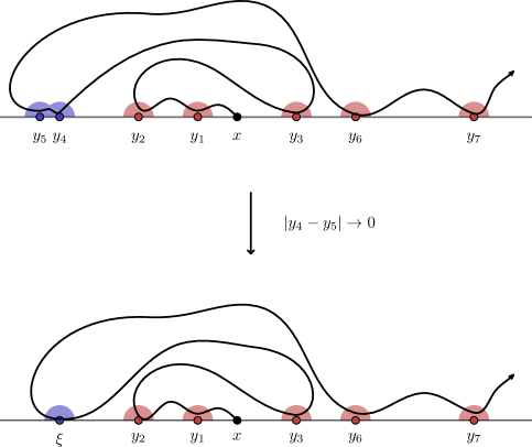
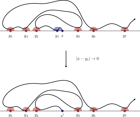
Our main result in the quantum group setup of the boundary visit problem is the existence of solutions to the system (5.2) – (5.5) and their uniqueness up to normalization. The proof is based on a number of observations made in Section 5.3, which are combined in Section 5.5.

Theorem 5.1.

There exists a unique collection $\left(\mathfrak{v}_{\omega}\right)_{\omega\in\mathrm{VO}}$ of vectors $\mathfrak{v}_{\omega}\in\mathsf{M}_{3}^{\otimes R(\omega)}\otimes\mathsf{M}_{2}\otimes\mathsf{M}_{3}^{\otimes L(\omega)}$ such that the system of equations (5.2) – (5.5) holds for all $\omega\in\mathrm{VO}$, with the normalization $\mathfrak{v}_{|N^{\prime}=0}=e_{0}\in\mathsf{M}_{2}$.

As a corollary, we obtain the existence of solutions to $\mathrm{SLE}$ boundary visit amplitudes for any number of visited points. For this one applies a slightly different “spin chain – Coulomb gas correspondence” $\mathcal{F}$ from $H_{2}(\mathsf{M}_{3}^{\otimes R}\otimes\mathsf{M}_{2}\otimes\mathsf{M}_{3}^{\otimes L})$ to functions of $L+R+1$ variables — see [KP14, JJK16] for details.

Theorem 5.2.

The collection $\left(\zeta_{\omega}\right)_{\omega\in\mathrm{VO}}$ of functions $\zeta_{\omega}=\mathcal{F}[\mathfrak{v}_{\omega}]$ satisfies the system of partial differential equations, covariance, and boundary conditions required in [JJK16], that is, the equations given in Figures 5.1, 5.2, and 5.3.

Proof.

Since the vectors $\mathfrak{v}_{\omega}$ satisfy (5.2), the functions $\zeta_{\omega}=\mathcal{F}[\mathfrak{v}_{\omega}]$ satisfy the PDEs and covariance given in Figure 5.1, by the (PDE) and (COV) parts of [KP14, Theorem 4.17]. The asymptotic conditions of Figures 5.2 and 5.3 follow from the projection conditions (5.3) – (5.5) for the vectors $\mathfrak{v}_{\omega}$, by the (ASY) part of [KP14, Theorem 4.17]. ∎

5.2. Link patterns associated to visiting orders

In Section 5.3, we construct solutions $\mathfrak{v}_{\omega}$ to the system (5.2) – (5.5). For a given visiting order $\omega$, the vector $\mathfrak{v}_{\omega}$ will be built from a vector $v_{\alpha}$ of Theorem 3.1, with an appropriately chosen link pattern $\alpha=\alpha(\omega)$. The mapping

(5.6) $$\qquad\omega\;\mapsto\;\alpha(\omega),\qquad\mathrm{VO}_{N^{\prime}}\;\rightarrow\;\mathrm{LP}_{N},$$

where $N=N^{\prime}+1=R(\omega)+L(\omega)+1$, associates to each visiting order $\omega=(\omega_{1},\ldots,\omega_{N^{\prime}})\in\mathrm{VO}_{N^{\prime}}$ a link pattern $\alpha(\omega)\in\mathrm{LP}_{N}$ as illustrated and explained in Figure 5.4, and defined in detail below.

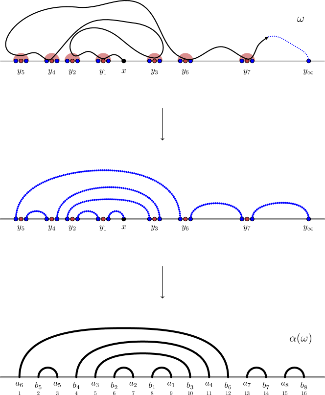
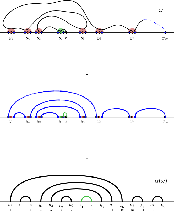
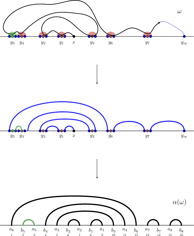
Let $\omega\in\mathrm{VO}_{N^{\prime}}$ and let $N=N^{\prime}+1$ and $L=L(\omega)$. Then $\alpha=\alpha(\omega)$ contains the $N$ links $[\wideparen{a_{1},b_{1}}],\ldots,[\wideparen{a_{N},b_{N}}]$, whose indices are defined recursively as follows. The index $a_{1}=2L+1$ corresponds to the starting point $x$, and $b_{1}=a_{1}+\omega_{1}$ corresponds to entering the first visited point $y_{1}$. For $j=2,\ldots,N^{\prime}+1$, the index $a_{j}=b_{j-1}+\omega_{j-1}$ corresponds to exiting the point $y_{j-1}$. Also, for $j=2,\ldots,N^{\prime}$, the index $b_{j}$ corresponds to entering the point $y_{j}$: if $\omega_{j}=+$ then $b_{j}=\max\left\{a_{1},a_{2},\ldots,a_{j-1}\right\}+1$, and if $\omega_{j}=-$ then $b_{j}=\min\left\{a_{1},a_{2},\ldots,a_{j-1}\right\}-1$. Finally, we also set $b_{N}=2N$, which corresponds to entering an auxiliary point $y_{\infty}$ — see Figure 5.4. It is straightforward to check that this defines a link pattern $\alpha=\alpha(\omega)$.

Remark 5.3.

Recall that the projection conditions (5.3) – (5.5) are written in terms of a visiting order $\hat{\omega}$ obtained from $\omega$ by collapsing two successive visits into one, or collapsing the first visit with the starting point. From the definition of the map $\alpha\mapsto\alpha(\omega)$ of (5.6), it is easy to see that $\hat{\alpha}=\alpha(\hat{\omega})$ is obtained from $\alpha=\alpha(\omega)$ by removing one link. More precisely, in the notation used in the above definition, the two cases are the following. For the case (5.5) of collapsing the first visit, we have

$$\hat{\omega} \;=(\omega_{2},\omega_{3},\ldots,\omega_{N^{\prime}})\qquad\qquad\qquad\text{ and} \alpha(\hat{\omega}) \;=\alpha(\omega)/[\wideparen{a_{1},b_{1}}],$$

see also Figure 5.5. For the case (5.3) of collapsing the $m$:th and $m+1$:st visit on the right, we have

$$\hat{\omega} \;=(\omega_{1},\ldots,\omega_{j-1},\omega_{j+1},\ldots,\omega_{N^{\prime}})\qquad\qquad\text{ and} \alpha(\hat{\omega}) \;=\alpha(\omega)/[\wideparen{a_{j+1},b_{j+1}}],$$

where the index $j$ is such that $\omega_{j}=\omega_{j+1}=+$ and $\#\left\{i\in\left\{1,\ldots,j\right\}\,\Big{|}\,\omega_{i}=+\right\}=m$. For the case of $m$:th and $m+1$:st visit on the left instead, the choice of $j$ is modified accordingly. See also Figure 5.6.

Figure 5.4. The mapping $\omega\mapsto\alpha(\omega)$ of (5.6) can be described as follows. Think of the visiting orders as planar connectivities of $N^{\prime}+1$ points, where small neighborhoods of the visited points $y_{j}$ have two lines attached to them, the starting point $x$ has one line attached, and every line is connected to another line so that no lines of the same point are connected (no loops). We open up the connectivity corresponding to the visiting order $\omega$: replace the points $y_{j}$ having two lines attached by two points, each having just one line attached. After this procedure, there will be one leftover line, attached to the last visited point (i.e. one of the two points by which we replaced the last visited point). We add a point $y_{\infty}$ to the right side of all other points, and connect the leftover line to this point. Finally, we label the endpoints of the links from left to right appropriately, to correspond with the labels of the endpoints of a link pattern $\alpha(\omega)$ in $\mathrm{LP}_{N}$.

Figure 5.5. Collapsing the first visited point: the effect on the link pattern $\alpha(\omega)$. In the example depicted in this figure, we have $\omega_{1}=-$, and the green link $[\wideparen{b_{1},a_{1}}]=[\wideparen{8,9}]$ is to be removed.

Figure 5.6. Collapsing two successive visits on the same side: the effect on the link pattern $\alpha(\omega)$. In the example depicted in this figure, the collapsed visits $y_{4},y_{5}$ are the third and fourth visits on the left, and the green link $[\wideparen{b_{5},a_{5}}]=[\wideparen{2,3}]$ is to be removed.

5.3. Construction of solutions

Recall from Lemma 2.1 that $\mathsf{M}_{2}\otimes\mathsf{M}_{2}\cong\mathsf{M}_{1}\oplus\mathsf{M}_{3}$. In this section, we use projections to these two irreducible subrepresentations. We identify the subrepresentations with $\mathsf{M}_{3}$ and $\mathsf{M}_{1}\cong\mathbb{C}$ by using the highest weight vectors $\tau_{0}^{(3;2,2)}$ and $\tau_{0}^{(1;2,2)}$ from (2.3). We thus define projections composed with the identifications as

$$\hat{\pi}^{(3)}\colon\; \mathsf{M}_{2}\otimes\mathsf{M}_{2}\rightarrow\mathsf{M}_{3}, \hat{\pi}^{(3)}(\tau_{l}^{(3;2,2)}) \;=e_{l}^{(3)}\qquad\text{for }l=0,1,2,\qquad$$

$$\hat{\pi}^{(1)}\colon\; \mathsf{M}_{2}\otimes\mathsf{M}_{2}\rightarrow\mathbb{C}, \hat{\pi}^{(1)}(\tau_{0}^{(1;2,2)}) \;=1.$$

We trust that no confusion arises, although the notation $\hat{\pi}^{(3)}$ coincides with that introduced in Section 5.1, since the two projections are defined on different spaces. We also denote by

$$\iota^{(3)}\colon\mathsf{M}_{3}\hookrightarrow\mathsf{M}_{2}\otimes\mathsf{M}_{2}$$

the embedding of the three dimensional subrepresentation into the tensor product $\mathsf{M}_{2}\otimes\mathsf{M}_{2}$ such that $\iota^{(3)}(e_{l}^{(3)})=\tau_{l}^{(3;2,2)}$, and thus, $\hat{\pi}^{(3)}\circ\iota^{(3)}=\mathrm{id}$.

Given a visiting order $\omega\in\mathrm{VO}_{N^{\prime}}$ with $L(\omega)=L$ and $R(\omega)=R$, the vector $\mathfrak{v}_{\omega}$ satisfying (5.2) – (5.5) will be constructed from the vector $v_{\alpha(\omega)}\in\mathsf{H}_{1}(\mathsf{M}_{2}^{\otimes 2N})$. The construction, $\mathfrak{v}_{\omega}=R_{+}\big{(}\widehat{\mathfrak{p}}_{L,R}(v_{\alpha(\omega)})\big{)}$, is summarized in the following diagram:

where the notations are defined below. The projection $\widehat{\mathfrak{p}}_{L,R}$ and embedding $\mathfrak{I}_{L,R}$ are defined by

$$\widehat{\mathfrak{p}}_{L,R}= \;\mathrm{id}\otimes(\hat{\pi}^{(3)})^{\otimes R}\otimes\mathrm{id}\otimes(\hat{\pi}^{(3)})^{\otimes L}, \mathfrak{I}_{L,R}= \;\mathrm{id}\otimes(\iota^{(3)})^{\otimes R}\otimes\mathrm{id}\otimes(\iota^{(3)})^{\otimes L},$$

$$\widehat{\mathfrak{p}}_{L,R}\colon \;\mathsf{M}_{2}^{\otimes 2N}\longrightarrow\mathsf{M}_{2}\otimes\mathsf{M}_{3}^{\otimes R}\otimes\mathsf{M}_{2}\otimes\mathsf{M}_{3}^{\otimes L}, \mathfrak{I}_{L,R}\colon \;\mathsf{M}_{2}\otimes\mathsf{M}_{3}^{\otimes R}\otimes\mathsf{M}_{2}\otimes\mathsf{M}_{3}^{\otimes L}\longrightarrow\mathsf{M}_{2}^{\otimes 2N},$$

and we denote $\widehat{\mathfrak{p}}_{L,R}(v_{\alpha(\omega)})=\mathfrak{v}_{\omega}^{\infty}$. The notation

$$\mathsf{H}_{1}\left(\mathsf{M}_{2}\otimes\mathsf{M}_{3}^{\otimes R}\otimes\mathsf{M}_{2}\otimes\mathsf{M}_{3}^{\otimes L}\right)\;=\;\left\{v\in\mathsf{M}_{2}\otimes\mathsf{M}_{3}^{\otimes R}\otimes\mathsf{M}_{2}\otimes\mathsf{M}_{3}^{\otimes L}\;\big{|}\;E.v=0,\;K.v=v\right\}$$

is used for the trivial subrepresentation. Finally, it can be shown, see [KP14, Lemma 5.3], that for any vector $v\in\mathsf{H}_{1}\left(\mathsf{M}_{2}\otimes\mathsf{M}_{3}^{\otimes R}\otimes\mathsf{M}_{2}\otimes\mathsf{M}_{3}^{\otimes L}\right)$ there exists a unique vector $\tau_{0}^{+}\in\mathsf{H}_{2}(\mathsf{M}_{3}^{\otimes R}\otimes\mathsf{M}_{2}\otimes\mathsf{M}_{3}^{\otimes L})$ such that

$$v=-q\;e_{0}^{(2)}\otimes F.\tau_{0}^{+}+e_{1}^{(2)}\otimes\tau_{0}^{+}.$$

This defines a linear isomorphism $R_{+}\colon v\mapsto\tau_{0}^{+}$ by [KP14, Lemma 5.3].

Remark 5.4.

By construction, the vector $\mathfrak{v}_{\omega}=R_{+}\big{(}\widehat{\mathfrak{p}}_{L,R}(v_{\alpha(\omega)})\big{)}$ satisfies the conditions (5.2). It remains to check that also the conditions (5.3) – (5.5) are satisfied.

Lemma 5.5.

The image of $\mathsf{H}_{1}\left(\mathsf{M}_{2}\otimes\mathsf{M}_{3}^{\otimes R}\otimes\mathsf{M}_{2}\otimes\mathsf{M}_{3}^{\otimes L}\right)$ under the embedding $\mathfrak{I}_{L,R}$ is the space

(5.7) $$\left\{v\in\mathsf{H}_{1}(\mathsf{M}_{2}^{\otimes 2N})\;\Big{|}\;\hat{\pi}^{(1)}_{2L+1-2m}(v)=0\text{ for }m=1,\ldots,L\;\text{ and }\;\hat{\pi}^{(1)}_{2L+2m^{\prime}}(v)=0\text{ for }m^{\prime}=1,\ldots,R\right\}.$$

The projection $\widehat{\mathfrak{p}}_{L,R}$ restricted to this space is a bijection onto $\mathsf{H}_{1}\left(\mathsf{M}_{2}\otimes\mathsf{M}_{3}^{\otimes R}\otimes\mathsf{M}_{2}\otimes\mathsf{M}_{3}^{\otimes L}\right)$, and its inverse is $\mathfrak{I}_{L,R}$. The vector $v_{\alpha(\omega)}$ lies in (5.7), and in particular, $\mathfrak{I}_{L,R}\big{(}\widehat{\mathfrak{p}}_{L,R}(v_{\alpha(\omega)})\big{)}=\mathfrak{I}_{L,R}(\mathfrak{v}_{\omega}^{\infty})=v_{\alpha(\omega)}$.

Proof.

The statements about the image of $\mathfrak{I}_{L,R}$ and restriction of $\widehat{\mathfrak{p}}_{L,R}$ are clear from the decomposition $\mathsf{M}_{2}\otimes\mathsf{M}_{2}\cong\mathsf{M}_{1}\oplus\mathsf{M}_{3}$. By definition of the mapping $\omega\mapsto\alpha(\omega)$, the link pattern $\alpha(\omega)$ does not contain links of type $[\wideparen{j,j+1}]$ where $j$ and $j+1$ correspond to the same visited point, i.e., $j=2L+1-2m$ or $j=2L+2m^{\prime}$. By the projection conditions (3.3) for $v_{\alpha(\omega)}$, we have $\hat{\pi}_{j}(v_{\alpha(\omega)})=0$ for all such $j$. ∎

We next show how the projections appearing in the conditions (5.3) – (5.5), acting on the vector $\mathfrak{v}_{\omega}$, can be expressed in terms of singlet projections $\hat{\pi}^{(1)}_{j}$ acting on the vector $v_{\alpha(\omega)}$. This will be done in three separate cases, corresponding to the three projection conditions (5.3) – (5.5), in the form of commutative diagrams in Lemmas 5.6, 5.8 and 5.10. Using these commutative diagrams, we then deduce the desired properties of the vector $\mathfrak{v}_{\omega}$ from the projection properties (3.3) of $v_{\alpha(\omega)}$, in Corollaries 5.7, 5.9 and 5.11.

Let $C_{2}=\frac{\left[2\right]^{2}}{\left[3\right]}$, and note that $C_{2}\neq 0$, since $q$ is not a root of unity.

Lemma 5.6.

For any $v\in\mathsf{M}_{3}\otimes\mathsf{M}_{2}$, we have $\hat{\pi}^{(2)}(v)=C_{2}\times\big{(}(\mathrm{id}\otimes\hat{\pi}^{(1)})\circ(\iota^{(3)}\otimes\mathrm{id})\big{)}(v)$, and for any $v\in\mathsf{M}_{2}\otimes\mathsf{M}_{3}$, we have $\hat{\pi}^{(2)}(v)=C_{2}\times\big{(}(\hat{\pi}^{(1)}\otimes\mathrm{id})\circ(\mathrm{id}\otimes\iota^{(3)}\big{)}(v)$. In other words, the following diagrams commute, up to the non-zero multiplicative constant $C_{2}$:

Proof.

We show the commutativity of the left diagram — the right is similar. Since the multiplicity of the subrepresentation $\mathsf{M}_{2}$ in $\mathsf{M}_{3}\otimes\mathsf{M}_{2}$ is one, by Schur’s lemma it suffices to show that the map $(\mathrm{id}\,\otimes\,\hat{\pi}^{(1)})\circ(\iota^{(3)}\,\otimes\,\mathrm{id})$ is non-zero. The vector

$$\tau_{0}^{(2;2,3)}=\frac{q^{2}}{1-q^{2}}\,e_{0}^{(3)}\otimes e_{1}^{(2)}\,+\,\frac{q^{2}}{q^{4}-1}\,e_{1}^{(3)}\otimes e_{0}^{(2)}$$

satisfies $\hat{\pi}^{(2)}(\tau_{0}^{(2;2,3)})=e_{0}^{(2)}\in\mathsf{M}_{2}$, by definition. Using Lemma 2.3(a) and the basis (2.6), we calculate

$$(\mathrm{id}\,\otimes\,\hat{\pi}^{(1)})\circ(\iota^{(3)}\,\otimes\,\mathrm{id})(\tau_{0}^{(2;2,3)})=\, (\mathrm{id}\,\otimes\,\hat{\pi}^{(1)})\left(\frac{q^{2}}{1-q^{2}}\,\tau^{(3;2,2)}_{0}\otimes e_{1}^{(2)}\,+\,\frac{q^{2}}{q^{4}-1}\,\tau^{(3;2,2)}_{1}\otimes e_{0}^{(2)}\right)$$

$$=\, \frac{\left[3\right]}{\left[2\right]^{2}}\times e_{0}^{(2)}=\frac{1}{C_{2}}\times e_{0}^{(2)}\neq 0.$$

∎

Corollary 5.7.

The vector $\mathfrak{v}_{\omega}=R_{+}\big{(}\widehat{\mathfrak{p}}_{L,R}(v_{\alpha(\omega)})\big{)}$ satisfies the conditions (5.5).

Proof.

The conditions (5.5) for the vector $\mathfrak{v}_{\omega}$ concern projections $\hat{\pi}^{(2)}_{\pm}$ acting on $\mathsf{M}_{3}\otimes\mathsf{M}_{2}$ and $\mathsf{M}_{2}\otimes\mathsf{M}_{3}$ in the middle of the tensor product (5.1). The linear isomorphism $R_{+}$ commutes with these projections, by [KP14, Eq. (5.2)]. Therefore, it suffices to consider the corresponding projection conditions for $\mathfrak{v}_{\omega}^{\infty}$. By Lemma 5.5, we have $v_{\alpha(\omega)}=\mathfrak{I}_{L,R}(\mathfrak{v}_{\omega}^{\infty})$. The projections $\hat{\pi}^{(2)}_{\pm}$ acting on $\mathfrak{v}_{\omega}^{\infty}$ can be calculated using the right columns of the commutative diagrams in Lemma 5.6, and the projections $\hat{\pi}^{(1)}_{2L}$ and $\hat{\pi}^{(1)}_{2L+1}$, acting on $v_{\alpha(\omega)}$, by the left columns. The assertion follows by observing that, by Remark 5.3 and (3.3), we have

$$\hat{\pi}^{(1)}_{2L}(v_{\alpha(\omega)})=\; \begin{cases}0\quad&\text{if }\omega_{1}=+\\ v_{\alpha(\hat{\omega})}&\text{if }\omega_{1}=-\end{cases}\qquad\qquad\Rightarrow\qquad\qquad\hat{\pi}^{(2)}_{-}(\mathfrak{v}_{\omega})=\; \begin{cases}0\quad&\text{if }\omega_{1}=+\\ C_{2}\times\mathfrak{v}_{\hat{\omega}}&\text{if }\omega_{1}=-\end{cases}$$

$$\hat{\pi}^{(1)}_{2L+1}(v_{\alpha(\omega)})=\; \begin{cases}v_{\alpha(\hat{\omega})}&\text{if }\omega_{1}=+\\ 0\quad&\text{if }\omega_{1}=-\end{cases}\qquad\qquad\Rightarrow\qquad\qquad\hat{\pi}^{(2)}_{+}(\mathfrak{v}_{\omega})=\; \begin{cases}C_{2}\times\mathfrak{v}_{\hat{\omega}}&\text{if }\omega_{1}=+\\ 0\quad&\text{if }\omega_{1}=-,\end{cases}$$

where $\hat{\omega}=(\omega_{2},\omega_{3},\ldots\omega_{N^{\prime}})$ is the order obtained from $\omega$ by collapsing the first visit. See also Figure 5.5. ∎

Let $C_{3}=\frac{\left[2\right]^{2}}{q^{2}+q^{-2}}$, and note that $C_{3}\neq 0$, since $q$ is not a root of unity.

Lemma 5.8.

For any $v\in\mathsf{M}_{3}\otimes\mathsf{M}_{3}$, we have $\hat{\pi}^{(3)}(v)=C_{3}\times\big{(}\hat{\pi}^{(3)}\circ(\mathrm{id}\otimes\hat{\pi}^{(1)}\otimes\mathrm{id})\circ(\iota^{(3)}\otimes\iota^{(3)})\big{)}(v)$. In other words, the following diagram commutes, up to the non-zero multiplicative constant $C_{3}$:

Proof.

The proof is similar to the proof of Lemma 5.6. One uses Schur’s lemma and concludes by calculating that the vector $\tau_{0}^{(3;3,3)}$ maps to a non-zero multiple of $e_{0}^{(3)}\in\mathsf{M}_{3}$ in the various mappings. ∎

Corollary 5.9.

The vector $\mathfrak{v}_{\omega}=R_{+}\big{(}\widehat{\mathfrak{p}}_{L,R}(v_{\alpha(\omega)})\big{)}$ satisfies the conditions (5.4).

Proof.

The conditions (5.4) for the vector $\mathfrak{v}_{\omega}$ concern projections $\hat{\pi}^{(3)}_{\epsilon;m}$ for the $m$:th and $m+1$:st points on the right ($\epsilon=+$) or left ($\epsilon=-$), acting on an appropriate pair $\mathsf{M}_{3}\otimes\mathsf{M}_{3}$ of consecutive tensor components of (5.1). Again, it suffices to prove the corresponding conditions for $\mathfrak{v}_{\omega}^{\infty}$. The projections $\hat{\pi}^{(3)}_{\epsilon;m}$ acting on $\mathfrak{v}_{\omega}^{\infty}$ can be calculated using the right column of the commutative diagram in Lemma 5.8, and the corresponding projections $\hat{\pi}^{(1)}_{k(\epsilon;m)}$, acting on $v_{\alpha(\omega)}$, using the left column (the index $k(\epsilon;m)$ is determined by $\epsilon$ and $m$). The assertion follows by observing that, by Remark 5.3 and (3.3), we have

$$\hat{\pi}^{(1)}_{k(\epsilon;m)}(v_{\alpha(\omega)})=\; \begin{cases}0&\mbox{in the case of non-successive visits }\\ v_{\alpha(\hat{\omega})}&\mbox{in the case of successive visits }\end{cases}$$

$$\qquad\qquad\Rightarrow\qquad\hat{\pi}^{(3)}_{\epsilon;m}(\mathfrak{v}_{\omega})=\; \begin{cases}0&\mbox{in the case of non-successive visits}\\ C_{3}\times\mathfrak{v}_{\hat{\omega}}&\mbox{in the case of successive visits}\end{cases}$$

where $\hat{\omega}$ is the order obtained from $\omega$ by collapsing these successive visits. See also Figure 5.6. ∎

Lemma 5.10.

For any $v\in\mathsf{M}_{3}\otimes\mathsf{M}_{3}$, we have $\hat{\pi}^{(1)}(v)=C\times\big{(}\hat{\pi}^{(1)}\circ(\mathrm{id}\otimes\hat{\pi}^{(1)}\otimes\mathrm{id})\circ(\iota^{(3)}\otimes\iota^{(3)})\big{)}(v)$. In other words, the following diagram commutes, up to the non-zero multiplicative constant $C=\frac{\left[2\right]^{3}}{\left[3\right]}$:

Proof.

The proof is similar to the proof of Lemma 5.6. One uses Schur’s lemma and concludes by calculating that the vector $\tau_{0}^{(1;3,3)}$ maps to a non-zero multiple of $1\in\mathbb{C}\cong\mathsf{M}_{1}$ in the various mappings. ∎

Corollary 5.11.

The vector $\mathfrak{v}_{\omega}=R_{+}\big{(}\widehat{\mathfrak{p}}_{L,R}(v_{\alpha(\omega)})\big{)}$ satisfies the conditions (5.3).

Proof.

The conditions (5.3) for the vector $\mathfrak{v}_{\omega}$ concern projections $\hat{\pi}^{(1)}_{\epsilon;m}$ for the $m$:th and $m+1$:st points on the right ($\epsilon=+$) or left ($\epsilon=-$), acting on an appropriate pair $\mathsf{M}_{3}\otimes\mathsf{M}_{3}$ of consecutive tensor components of (5.1). Again, it suffices to prove the corresponding conditions for $\mathfrak{v}_{\omega}^{\infty}$. The projections $\hat{\pi}^{(1)}_{\epsilon;m}$ acting on $\mathfrak{v}_{\omega}^{\infty}$ can be calculated using the right column of the commutative diagram in Lemma 5.10, and the corresponding projections $\hat{\pi}^{(1)}_{k^{\prime}(\epsilon;m)}\circ\hat{\pi}^{(1)}_{k(\epsilon;m)}$, acting on $v_{\alpha(\omega)}$, using the left column (the indices $k(\epsilon;m)$ and $k^{\prime}(\epsilon;m)$ are determined by the indices $\epsilon$ and $m$). The link pattern $\alpha(\omega)$ cannot contain the two nested links $[\wideparen{k,k+1}]$ and $[\wideparen{k-1,k+2}]$ with $k=k(\epsilon;m)$. Hence, by (3.3), we have

$$\hat{\pi}^{(1)}_{k^{\prime}(\epsilon;m)}(\hat{\pi}^{(1)}_{k(\epsilon;m)}(v_{\alpha(\omega)}))=0.$$

∎

5.4. Uniqueness of solutions

The proof of the uniqueness of solutions of the system (5.2) – (5.5) is similar to the multiple $\mathrm{SLE}$ case (Proposition 3.2) — the homogeneous system only admits the trivial solution. We make use of the following lemma, which is a generalization of Corollary 2.5.

Lemma 5.12.

Let $L,R\in\mathbb{Z}_{\geq 0}$, $L+R\geq 1$, and assume that the vector $v\in\mathsf{M}_{3}^{\otimes R}\otimes\mathsf{M}_{2}\otimes\mathsf{M}_{3}^{\otimes L}$ satisfies $\,E.v=0\,$, $\,K.v=q\,v\,$, and $\,\hat{\pi}^{(2)}_{\pm}(v)=0\,$, and $\,\hat{\pi}^{(3)}_{\epsilon;m}(v)=0\,$, $\,\hat{\pi}^{(1)}_{\epsilon;m}(v)=0\,$ for all indices $m$ and $\epsilon=\pm$. Then we have $v=0$.

Proof.

The conditions $E.v=0$, $K.v=q\,v$ show that $v\in\mathsf{H}_{2}(\mathsf{M}_{3}^{\otimes R}\otimes\mathsf{M}_{2}\otimes\mathsf{M}_{3}^{\otimes L})$. Denote by

$$\widehat{\mathfrak{p}}_{L,R}^{\prime}=\; (\hat{\pi}^{(3)})^{\otimes R}\otimes\mathrm{id}\otimes(\hat{\pi}^{(3)})^{\otimes L}\;\colon\;\mathsf{M}_{2}^{\otimes(2N-1)}\longrightarrow\mathsf{M}_{3}^{\otimes R}\otimes\mathsf{M}_{2}\otimes\mathsf{M}_{3}^{\otimes L},$$

$$\mathfrak{I}_{L,R}^{\prime}=\; (\iota^{(3)})^{\otimes R}\otimes\mathrm{id}\otimes(\iota^{(3)})^{\otimes L}\;\colon\;\mathsf{M}_{3}^{\otimes R}\otimes\mathsf{M}_{2}\otimes\mathsf{M}_{3}^{\otimes L}\hookrightarrow\mathsf{M}_{2}^{\otimes(2N-1)},$$

$$v^{\prime}=\; \mathfrak{I}_{L,R}^{\prime}(v)\;\in\;\mathsf{H}_{2}(\mathsf{M}_{2}^{\otimes(2N-1)}):=\left\{v\in\mathsf{M}_{2}^{\otimes(2N-1)}\;\big{|}\;E.v=0,\;K.v=qv\right\}.$$

The assumptions $\,\hat{\pi}^{(2)}_{\pm}(v)=0\,$, $\,\hat{\pi}^{(3)}_{\epsilon;m}(v)=0\,$, $\,\hat{\pi}^{(1)}_{\epsilon;m}(v)=0\,$ for all indices $m$ and $\epsilon$ imply that in the direct sum decomposition of any two consecutive tensorands ($\mathsf{M}_{3}\otimes\mathsf{M}_{3}$, $\mathsf{M}_{2}\otimes\mathsf{M}_{3}$ or $\mathsf{M}_{3}\otimes\mathsf{M}_{2}$) of the tensor product (5.1) into irreducibles, the vector $v$ lies in the highest dimensional subrepresentation. An application of Lemma 2.4 to each pair of two consecutive tensorands embedded in a tensor product of two dimensional representations ($\mathsf{M}_{3}\otimes\mathsf{M}_{3}$ via $\iota^{(3)}\otimes\iota^{(3)}$, $\mathsf{M}_{2}\otimes\mathsf{M}_{3}$ via $\mathrm{id}\otimes\iota^{(3)}$, and $\mathsf{M}_{3}\otimes\mathsf{M}_{2}$ via $\iota^{(3)}\otimes\mathrm{id}$) shows that $\hat{\pi}^{(1)}_{j}(v^{\prime})=0$ for all $1\leq j\leq 2N-2$. Therefore, by Lemma 2.4 applied to $\mathsf{M}_{2}^{\otimes(2N-1)}$, the vector $v^{\prime}$ belongs to the highest dimensional subrepresentation $\mathsf{M}_{2N}\subset\mathsf{M}_{2}^{\otimes(2N-1)}$. Hence, we have $v^{\prime}\in\mathsf{M}_{2N}\cap\mathsf{M}_{2}=\{0\}$, as $N=R+L+1\geq 2$. We conclude by $v=\widehat{\mathfrak{p}}_{L,R}^{\prime}(v^{\prime})=0$. ∎

5.5. Proof of Theorem 5.1

Solutions to (5.2) – (5.5) were constructed in Section 5.3 — see Remark 5.4 and Corollaries 5.7, 5.9 and 5.11. Uniqueness of normalized solutions follows from Lemma 5.12 similarly as in the proof of Proposition 3.2: the difference of any two solutions of (5.2) – (5.5) vanishes as a solution to the homogeneous system, which appears in the statement of the lemma. $\hfill\qed$

Appendix A Local multiple $\mathrm{SLE}$s

The key technique to construct $\mathrm{SLE}$ type curves is their description as growth processes [Sch00]. Growth processes for multiple curves, however, straightforwardly only allow to construct initial segments of the curves. In this article we restrict our attention to such local multiple $\mathrm{SLE}$s. In extending the definition to a probability measure on $N$ globally defined random curves connecting $2N$ boundary points, one encounters technical difficulties similar to the challenges in proving the reversibility property of a single chordal $\mathrm{SLE}$ curve [Zha08b, MS12b].

A.1. Chordal Schramm-Loewner evolution

The simplest $\mathrm{SLE}$ variant is the chordal $\mathrm{SLE}_{\kappa}$. Let $\Lambda\subset\mathbb{C}$ be an open simply connected domain, with two distinct boundary points $\xi,\eta\in\partial\Lambda$ (prime ends). The chordal $\mathrm{SLE}_{\kappa}$ in $\Lambda$ from $\xi$ to $\eta$ is a random curve — more precisely, a probability measure $\mathsf{P}^{(\Lambda;\xi,\eta)}_{\oslash}$ on oriented but unparametrized non-self-crossing curves in $\overline{\Lambda}$ from $\xi$ to $\eta$ (the space of such curves is equipped with a natural metric inherited from a uniform norm on parametrized curves). We often choose some parametrized curve $\gamma\colon[0,1]\to\overline{\Lambda}$, to be interpreted as its equivalence class under increasing reparametrizations. The chordal $\mathrm{SLE}_{\kappa}$ itself is the family $\big{(}\mathsf{P}^{(\Lambda;\xi,\eta)}_{\oslash}\big{)}_{\Lambda,\xi,\eta}$ of these probability measures, indexed by the domain and marked boundary points. Schramm’s observation was that, up to the value of the parameter $\kappa>0$, the family is characterized by the following two assumptions.

• Conformal invariance: If $\phi\colon\Lambda\to\Lambda^{\prime}$ is a conformal map, and the curve $\gamma$ in $\Lambda$ has the law $\mathsf{P}^{(\Lambda;\xi,\eta)}_{\oslash}$, then the image $\phi\circ\gamma$ has the law $\mathsf{P}_{\oslash}^{(\phi(\Lambda);\phi(\xi),\phi(\eta))}$. A concise way to state this is that the measures are related by pushforwards, $\phi_{*}\mathsf{P}_{\oslash}^{(\Lambda;\xi,\eta)}=\mathsf{P}_{\oslash}^{(\phi(\Lambda);\phi(\xi),\phi(\eta))}$.

• Domain Markov property: Conditionally, given an initial segment $\gamma|_{[0,\tau]}$ of the curve $\gamma$ with law $\mathsf{P}_{\oslash}^{(\Lambda;\xi,\eta)}$, the remaining part $\gamma|_{[\tau,1]}$ has the law $\mathsf{P}_{\oslash}^{(\Lambda^{\prime};\gamma(\tau),\eta)}$, where $\Lambda^{\prime}$ is the component of $\Lambda\setminus\gamma[0,\tau]$ containing $\eta$ on its boundary.

By Riemann mapping theorem, between any triples $(\Lambda;\xi,\eta)$ and $(\Lambda^{\prime};\xi^{\prime},\eta^{\prime})$ there exists a conformal map $\phi\colon\Lambda\to\Lambda^{\prime}$ such that $\phi(\xi)=\xi^{\prime}$, $\phi(\eta)=\eta^{\prime}$. By conformal invariance, it therefore suffices to construct the chordal $\mathrm{SLE}_{\kappa}$ in one reference domain, e.g., the upper half-plane

$$\mathbb{H}=\left\{z\in\mathbb{C}\;\big{|}\;\Im\mathfrak{m}(z)>0\right\}.$$

The chordal $\mathrm{SLE}_{\kappa}$ in $(\Lambda;\xi,\eta)=(\mathbb{H};0,\infty)$ is constructed by a growth process encoded in a Loewner chain $(g_{t})_{t\in[0,\infty)}$ as follows — see [RS05] for details. Let $(B_{t})_{t\in[0,\infty)}$ be a standard Brownian motion on the real line, and for $z\in\mathbb{H}$, consider the solution to the Loewner differential equation

(A.1) $$\frac{\mathrm{d}}{\mathrm{d}t}g_{t}(z)=\frac{2}{g_{t}(z)-D_{t}},\qquad g_{0}(z)=z,$$

with the driving function $D_{t}=\sqrt{\kappa}B_{t}$. The solution is defined up to a (possibly infinite) explosion time $T_{z}$. Let $K_{t}$ be the closure of the set $\left\{z\in\mathbb{H}\;|\;T_{z}<t\right\}$. The growth process $(K_{t})_{t\in[0,\infty)}$ is generated by a random curve $\gamma\colon[0,\infty)\to\overline{\mathbb{H}}$ in the sense that $\mathbb{H}\setminus K_{t}$ is the unbounded component of $\mathbb{H}\setminus\gamma[0,t]$. This curve is (a parametrization of) the chordal $\mathrm{SLE}_{\kappa}$. For fixed $t\in[0,\infty)$, the solution to (A.1) viewed as a function of the initial condition $z$ gives the unique conformal map $g_{t}\colon\mathbb{H}\setminus K_{t}\rightarrow\mathbb{H}$ normalized so that $g_{t}(z)=z+\mathit{o}(1)$ as $z\to\infty$.

A.2. Local multiple $\mathrm{SLE}$s

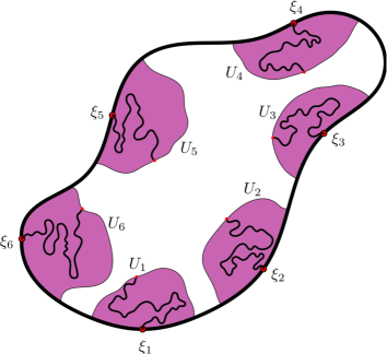
Let $\Lambda\subsetneq\mathbb{C}$ be a simply connected domain, and let $\xi_{1},\ldots,\xi_{2N}\in\partial\Lambda$ be $2N$ distinct boundary points appearing in counterclockwise order along $\partial\Lambda$. Morally, we would like to associate to the domain and boundary points a probability measure $\mathsf{P}^{(\Lambda;\xi_{1},\ldots,\xi_{2N})}$ on a collection of $N$ curves, connecting the $2N$ marked boundary points. Instead, a local multiple $\mathrm{SLE}$ will describe $2N$ initial segments $\gamma^{(j)}$ of curves starting from the points $\xi_{j}$, up to exiting some neighborhoods $U_{j}\ni\xi_{j}$. The localization neighborhoods $U_{1},\ldots,U_{2N}$ are assumed to be closed subsets of $\overline{\Lambda}$ such that $\Lambda\setminus U_{j}$ are simply connected and $U_{j}\cap U_{k}=\emptyset$ for $j\neq k$. See Figure A.1 for an illustration of the localization.

The local $N$-$\mathrm{SLE}_{\kappa}$ in $\Lambda$, started from $(\xi_{1},\ldots,\xi_{2N})$ and localized in $(U_{1},\ldots,U_{2N})$, is a probability measure on $2N$-tuples of oriented unparametrized curves with parametrized representatives $(\gamma^{(1)},\ldots,\gamma^{(2N)})$, such that for each $j$, the curve $\gamma^{(j)}\colon[0,1]\to U_{j}$ starts at $\gamma^{(j)}(0)=\xi_{j}$ and ends at $\gamma^{(j)}(1)\in\partial(\Lambda\setminus U_{j})$ on the boundary of the localization neighborhood. The local $N$-$\mathrm{SLE}_{\kappa}$ itself is the indexed collection

$$\mathsf{P}=\left(\mathsf{P}^{(\Lambda;\xi_{1},\ldots,\xi_{2N})}_{(U_{1},\ldots,U_{2N})}\right)_{\Lambda;\xi_{1},\ldots,\xi_{2N};U_{1},\ldots,U_{2N}}.$$

This collection of probability measures is required to satisfy conformal invariance, domain Markov property, and absolute continuity of marginals with respect to the chordal $\mathrm{SLE}_{\kappa}$:

(CI):

If $\phi:\Lambda\rightarrow\Lambda^{\prime}$ is a conformal map, then the measures are related by pushforward,

$$\phi_{*}\mathsf{P}^{(\Lambda;\xi_{1},\ldots,\xi_{2N})}_{(U_{1},\ldots,U_{2N})}=\mathsf{P}^{(\phi(\Lambda);\phi(\xi_{1}),\ldots,\phi(\xi_{2N}))}_{(\phi(U_{1}),\ldots,\phi(U_{2N}))}.$$

(DMP):

Conditionally, given initial segments $\gamma^{(j)}|_{[0,\tau_{j}]}$ of the curves $(\gamma^{(1)},\ldots,\gamma^{(2N)})$ with law $\mathsf{P}^{(\Lambda;\xi_{1},\ldots,\xi_{2N})}_{(U_{1},\ldots,U_{2N})}$, the remaining parts $(\gamma^{(1)}|_{[\tau_{1},1]},\ldots,\gamma^{(2N)}|_{[\tau_{2N},1]})$ have the law $\mathsf{P}^{(\Lambda^{\prime};\xi_{1}^{\prime},\ldots,\xi_{2N}^{\prime})}_{(U^{\prime}_{1},\ldots,U^{\prime}_{2N})}$, where $\Lambda^{\prime}$ is the component of $\Lambda\setminus\bigcup_{j=1}^{2N}\gamma^{(j)}[0,\tau_{j}]$ containing all tips $\xi_{j}^{\prime}=\gamma^{(j)}(\tau_{j})$ on its boundary, and $U^{\prime}_{j}=U_{j}\cap\Lambda^{\prime}$.

(MARG):

There exist smooth functions $b^{(j)}:\mathfrak{X}_{2N}\to\mathbb{R}$, for $j=1,\ldots,2N$, such that for the domain $\Lambda=\mathbb{H}$, boundary points $x_{1}<\ldots<x_{2N}$, and their localization neighborhoods $U_{1},\ldots,U_{2N}$, the marginal on the $j$:th curve $\gamma^{(j)}$ under $\mathsf{P}^{(\mathbb{H};x_{1},\ldots,x_{2N})}_{(U_{1},\ldots,U_{2N})}$ is the following. Consider the Loewner equation (A.1) with driving process $(X_{t})_{t\in[0,\sigma)}$ that solves the system of Itô SDEs

(A.2) $$\mathrm{d}X_{t}= \;\sqrt{\kappa}\,\mathrm{d}B_{t}\,+\,b^{(j)}(X^{(1)}_{t},\ldots,X^{(j-1)}_{t},X_{t},X^{(j+1)}_{t}\ldots,X^{(2N)}_{t})\,\mathrm{d}t$$

$$\mathrm{d}X^{(i)}_{t}= \;\frac{2\,\mathrm{d}t}{X^{(i)}_{t}-X_{t}}\qquad\text{for}\;i\neq j,$$

where $X_{0}=x_{j}$ and $X^{(i)}_{0}=x_{i}$ for $i\neq j$. As in the case of the chordal $\mathrm{SLE}{}_{\kappa}$, the solution ${g_{t}\colon\mathbb{H}\setminus K_{t}\to\mathbb{H}}$ to (A.1) is a conformal map, and the growth process $(K_{t})_{t\in[0,\sigma)}$ is generated by a curve $\gamma\colon[0,\sigma)\to\overline{\mathbb{H}}$. The processes (A.2) are defined at least up to the stopping time $\sigma_{j}=\inf\left\{t\geq 0\;\big{|}\;\gamma\in\partial(\mathbb{H}\setminus U_{j})\right\}$. The marginal law of $\gamma^{(j)}$ is that of the random curve $\gamma|_{[0,\sigma_{j}]}$.

Figure A.1. Schematic illustration of a local multiple $\mathrm{SLE}$.

We will use the following result of Dubédat.

Proposition A.1 ([Dub07]).

If $\mathsf{P}=\big{(}\mathsf{P}^{(\Lambda;\xi_{1},\ldots,\xi_{2N})}_{(U_{1},\ldots,U_{2N})}\big{)}$ satisfies the conditions (CI), (DMP), and (MARG), then there exists a function $\mathcal{Z}\colon\mathfrak{X}_{2N}\to\mathbb{R}_{>0}$ satisfying the partial differential equations (1.2), such that the drift functions in (MARG) take the form

$$b^{(j)}=\kappa\,\frac{\partial_{j}\mathcal{Z}}{\mathcal{Z}}\qquad\text{for}\;j=1,\ldots,2N.$$

Proof.

Given the local multiple $\mathrm{SLE}_{\kappa}$ $\mathsf{P}$, we may take $\Lambda=\mathbb{H}$ and any $(x_{1},\ldots,x_{2N})\in\mathfrak{X}_{2N}$. It follows from [Dub07, Theorem 7 and the remark after it] that there exists a function $\mathcal{Z}$ satisfying (1.2) such that the drifts in (A.2) are $b^{(j)}=\kappa\,\frac{\partial_{j}\mathcal{Z}}{\mathcal{Z}}$. The solution $\mathcal{Z}$ is a priori defined in a neighborhood of the starting point $(x_{1},\ldots,x_{2N})$, and determined only up to a multiplicative constant. By considering different starting points, we see that such a function $\mathcal{Z}\colon\mathfrak{X}_{2N}\rightarrow\mathbb{R}_{>0}$ exists on the entire chamber. ∎

We note that the localizations satisfy the following consistency property under restriction to smaller localization neighborhoods. This consistency allows always continuing the curves by a little, but it is not sufficient for the definition of a global multiple $\mathrm{SLE}$.

Proposition A.2.

Suppose that both $(U_{1},\ldots,U_{2N})$ and $(V_{1},\ldots,V_{2N})$ are localization neighborhoods for $(\Lambda;\xi_{1},\ldots,\xi_{2N})$, and that $V_{j}\subset U_{j}$ for each $j$. Let $(\gamma^{(1)},\ldots,\gamma^{(2N)})$ be representatives of curves with law $\mathsf{P}^{(\Lambda;\xi_{1},\ldots,\xi_{2N})}_{(U_{1},\ldots,U_{2N})}$, and let $\sigma_{j}=\inf\left\{t\geq 0\;\big{|}\;\gamma^{(j)}(t)\in\partial(\Lambda\setminus V_{j})\right\}$ be their exit times from the smaller neighborhoods. Then $(\gamma^{(1)}|_{[0,\sigma_{1}]},\ldots,\gamma^{(2N)}|_{[0,\sigma_{2N}]})$ are representatives of curves with law $\mathsf{P}^{(\Lambda;\xi_{1},\ldots,\xi_{2N})}_{(V_{1},\ldots,V_{2N})}$.

Proof.

The marginal on the $j$:th curve described in (MARG) clearly satisfies such a restriction consistency. The consistency for all curves follows inductively by the domain Markov property (DMP). ∎

A.3. Sampling one by one from marginals

Property (MARG) describes the marginal law of one of the $2N$ curves, and property (DMP) gives the conditional law of the others, given one. One thus obtains a procedure for sampling a local multiple $\mathrm{SLE}_{\kappa}$. In this section, we first describe the marginal law of $\gamma^{(j)}$ by its Radon-Nikodym derivative with respect to the chordal $\mathrm{SLE}_{\kappa}$, explicitly expressed in terms of $\mathcal{Z}$. We then formalize the sampling procedure, which is now meaningful with just the knowledge of $\mathcal{Z}$.

Recall that by Proposition A.1, the drift functions $b^{(j)}$ are necessarily of the form $b^{(j)}=\kappa\,\frac{\partial_{j}\mathcal{Z}}{\mathcal{Z}}$. Let $(X_{t})_{t\in[0,\tau]}$ and $\big{(}X^{(i)}_{t}\big{)}_{t\in[0,\tau]}$ for $i\neq j$ solve the SDEs (A.2) with these drifts, and let $\gamma\colon[0,\tau]\rightarrow\overline{\mathbb{H}}$ be the random curve with the Loewner driving function $X_{t}$ as in (MARG), and $\tau$ any stopping time such that, for some $\varepsilon>0$ and all $0\leq t\leq\tau$, we have

(A.3) $$|X^{(i)}_{t}-X^{(k)}_{t}|\geq\varepsilon\qquad\text{for all}\quad i\neq k\qquad\text{ and }\qquad|X^{(i)}_{t}-X_{t}|\geq\varepsilon\qquad\text{for all}\quad i.$$

Then, the law $\mathsf{P}_{\gamma}$ of the curve $\gamma$ is absolutely continuous with respect to an initial segment of the chordal $\mathrm{SLE}_{\kappa}$, with Radon-Nikodym derivative

(A.4) $$\frac{\mathrm{d}\mathsf{P}_{\gamma}}{\mathrm{d}\mathsf{P}_{\oslash}^{(\mathbb{H};X_{0},\infty)}}=\,\prod_{i\neq j}(g^{\prime}(X^{(i)}_{0}))^{h}\;\times\;\frac{\mathcal{Z}\big{(}g(X^{(1)}_{0}),\ldots,g(X^{(j-1)}_{0}),g(\gamma(\tau)),g(X^{(j+1)}_{0}),\ldots,g(X^{(2N)}_{0})\big{)}}{\mathcal{Z}\big{(}X^{(1)}_{0},\ldots,X^{(j-1)}_{0},X_{0},X^{(j+1)}_{0},\ldots,X^{(2N)}_{0}\big{)}},$$

where $g:\mathbb{H}\setminus K\to\mathbb{H}$ is the conformal map such that $g(z)=z+\mathit{o}(1)$ as $z\to\infty$, $K$ is the hull of $\gamma$ and $h=\frac{6-\kappa}{2\kappa}$. In fact, $\gamma$ is obtained by Girsanov re-weighting of the chordal $\mathrm{SLE}_{\kappa}$ by the martingale

(A.5) $$t\;\mapsto \;M_{t}$$

$$= \prod_{i\neq j}(g_{t}^{\prime}(X^{(i)}_{0}))^{h}\;\times\;\mathcal{Z}\Big{(}g_{t}(X^{(1)}_{0}),\ldots,g_{t}(X^{(j-1)}_{0}),\sqrt{\kappa}B_{t}+X_{0},g_{t}(X^{(j+1)}_{0}),\ldots,g_{t}(X^{(2N)}_{0})\Big{)}$$

where $g_{t}$ is the solution to the Loewner equation (A.1) with the driving function $D_{t}=\sqrt{\kappa}B_{t}+X_{0}$.

In view of the above, given points $X^{(1)}_{0}<\cdots<X^{(j-1)}_{0}<X_{0}<X^{(j+1)}_{0}<\cdots<X^{(2N)}_{0}$, a neighborhood $U$ of $X_{0}$ not containing the points $X^{(i)}_{0}$, and a positive function $\mathcal{Z}$, we construct a random curve $\gamma$ by the weighting (A.4) of an initial segment of the chordal $\mathrm{SLE}_{\kappa}$ up to the stopping time

$$\tau=\sigma^{(U)}=\inf\left\{t>0\;\big{|}\;\gamma(t)\in\partial(\mathbb{H}\setminus U)\right\}.$$

Note that this stopping time satisfies the condition (A.3), by standard harmonic measure estimates.

Sampling procedure A.3.

Given a positive function $\mathcal{Z}\colon\mathfrak{X}_{2N}\rightarrow\mathbb{R}_{>0}$, a random $2N$-tuple $(\gamma^{(1)},\ldots,\gamma^{(2N)})$ of curves in $\mathbb{H}$ starting from $(x_{1},\ldots,x_{2N})$ with localization neighborhoods $(U_{1},\ldots,U_{2N})$ can be sampled according to the following procedure.

• Select an order in which the curves will be sampled, encoded in a permutation $p\in\mathfrak{S}_{2N}$.

• Sample the first curve in the selected order, $\gamma^{(j)}$ for $j=p(1)$, from the measure (A.4) with $X_{0}=x_{j}$ and $X_{0}^{(i)}=x_{i}$ for $i\neq j$, and with the stopping time $\tau=\sigma^{(U_{j})}$.

• Suppose the first $k-1$ curves $\gamma^{(p(1))},\ldots,\gamma^{(p(k-1))}$ in the selected order have been sampled, and let $j=p(k)$. Let $K$ be the hull of $\gamma^{(p(1))}\cup\cdots\cup\gamma^{(p(k-1))}$, and $G\colon\mathbb{H}\setminus K\to\mathbb{H}$ the conformal map such that $G(z)=z+\mathit{o}(1)$ as $z\to\infty$. Let $X_{0}=G(x_{j})$, $X^{(p(i))}_{0}=G(x_{i})$ for $i=k+1,\ldots,2N$, and let $X^{(p(l))}_{0}$ be the image of the tip of $\gamma^{(p(l))}$ for $l=1,\ldots,k-1$. Construct the $k$:th curve as $\gamma^{(j)}=G^{-1}\circ\gamma$ using the curve $\gamma$ sampled from the measure (A.4) with the stopping time $\tau=\sigma^{(G(U_{j}))}$.

By the local commutation of Dubédat, [Dub07], this procedure results in the same law of $(\gamma^{(1)},\ldots,\gamma^{(2N)})$ independently of the sampling order $p$, provided that $\mathcal{Z}$ is a solution to the system (1.2).

A.4. Partition function and PDEs

We will next state the main theorem towards a construction of multiple $\mathrm{SLE}$ processes. The most profound parts of the proof rely on Dubédat’s commutation of $\mathrm{SLE}$s [Dub07]. In summary, the theorem states that multiple $\mathrm{SLE}_{\kappa}$ partition functions $\mathcal{Z}$ correspond to local multiple $\mathrm{SLE}_{\kappa}$ processes, via the sampling procedure A.3, and two partition functions correspond to the same local multiple $\mathrm{SLE}_{\kappa}$ if and only if they are proportional to each other. More precisely, the set

$$\left\{\mathcal{Z}(x_{1},\ldots,x_{2N})\;|\;\mathcal{Z}\colon\mathfrak{X}_{2N}\rightarrow\mathbb{R}_{>0}\;\text{is a positive solution to \eqref{eq: multiple SLE PDEs}\leavevmode\nobreak\ --\leavevmode\nobreak\ \eqref{eq: multiple SLE Mobius covariance}}\;\right\}\;\big{/}\;\mathbb{R}_{>0}$$

corresponds one-to-one with the set of local multiple $\mathrm{SLE}$s $\mathsf{P}$. Moreover, convex combinations of partition functions correspond to convex combinations of localizations of multiple $\mathrm{SLE}$s as probability measures.

Theorem A.4.

(a):

Suppose $\mathcal{Z}\colon\mathfrak{X}_{2N}\rightarrow\mathbb{R}_{>0}$ is a positive solution to the system (1.2) – (1.3). Then the random collection of curves obtained by Procedure A.3 is a local multiple $\mathrm{SLE}_{\kappa}$. Two functions $\mathcal{Z},\tilde{\mathcal{Z}}$ give rise to the same local multiple $\mathrm{SLE}_{\kappa}$ if and only if $\mathcal{Z}=\mathrm{const.}\times\tilde{\mathcal{Z}}$.

(b):

Suppose $\mathsf{P}$ is a local multiple $\mathrm{SLE}_{\kappa}$. Then there exists a positive solution $\mathcal{Z}\colon\mathfrak{X}_{2N}\rightarrow\mathbb{R}_{>0}$ to the system (1.2) – (1.3), such that for any $j=1,\ldots,2N$, the drift in (A.2) is given by $b^{(j)}=\kappa\,\frac{\partial_{j}\mathcal{Z}}{\mathcal{Z}}$. Such a function $\mathcal{Z}$ is determined up to a multiplicative constant.

(c):

Suppose that $\mathcal{Z}_{1}$ and $\mathcal{Z}_{2}$ are positive solutions to the system (1.2) – (1.3) and

$$\mathcal{Z}=r\,\mathcal{Z}_{1}+(1-r)\,\mathcal{Z}_{2},$$

with $0\leq r\leq 1$. Denote by $\;\mathsf{P}=\left(\mathsf{P}^{(\Lambda;\xi_{1},\ldots,\xi_{2N})}_{(U_{1},\ldots,U_{2N})}\right)$, $\mathsf{P}_{1}=\left((\mathsf{P}_{1})^{(\Lambda;\xi_{1},\ldots,\xi_{2N})}_{(U_{1},\ldots,U_{2N})}\right)$ and $\mathsf{P}_{2}=\left((\mathsf{P}_{2})^{(\Lambda;\xi_{1},\ldots,\xi_{2N})}_{(U_{1},\ldots,U_{2N})}\right)$ the local multiple $\mathrm{SLE}$s associated to $\mathcal{Z}$, $\mathcal{Z}_{1}$ and $\mathcal{Z}_{2}$, respectively. Fix the domain $\Lambda$ and the marked points $(\xi_{1},\ldots,\xi_{2N})$, and let $(U_{1},\ldots,U_{2N})$ be any localization neighborhoods. Then the probability measure associated to $\mathcal{Z}$ is obtained as the following convex combination

(A.6) $$\mathsf{P}^{(\Lambda;\xi_{1},\ldots,\xi_{2N})}_{(U_{1},\ldots,U_{2N})}\;= \;r\,\frac{\mathcal{Z}_{1}(\phi(\xi_{1}),\ldots,\phi(\xi_{2N}))}{\mathcal{Z}(\phi(\xi_{1}),\ldots,\phi(\xi_{2N}))}\;(\mathsf{P}_{1})^{(\Lambda;\xi_{1},\ldots,\xi_{2N})}_{(U_{1},\ldots,U_{2N})}\,$$

$$+\,(1-r)\,\frac{\mathcal{Z}_{2}(\phi(\xi_{1}),\ldots,\phi(\xi_{2N}))}{\mathcal{Z}(\phi(\xi_{1}),\ldots,\phi(\xi_{2N}))}\;(\mathsf{P}_{2})^{(\Lambda;\xi_{1},\ldots,\xi_{2N})}_{(U_{1},\ldots,U_{2N})},$$

where $\phi\colon\Lambda\rightarrow\mathbb{H}$ is any conformal map such that $\phi^{-1}(\infty)$ belongs to the positively oriented boundary segment between $\xi_{2N}$ and $\xi_{1}$.

Proof.

(a):

In $\mathbb{H}$, for any marked points $(x_{1},\ldots,x_{2N})$ and localization neighborhoods $(U_{1},\ldots,U_{2N})$, Procedure A.3 defines a random $2N$-tuple $(\gamma^{(1)},\ldots,\gamma^{(2N)})$ of curves. From the assumption (1.2) and the local commutation of [Dub07, Lemma 6 & Theorem 7] it follows that the law of $(\gamma^{(1)},\ldots,\gamma^{(2N)})$ is independent of the chosen sampling order $p$. From the assumption (1.3) and a standard coordinate change [Kyt07, Proposition 6.1] it follows that the result of the sampling is Möbius invariant, that is, (CI) holds for any $\phi\colon\mathbb{H}\rightarrow\mathbb{H}$ which preserves the order of the marked points. Thus, we may use (CI) to define the laws of the random $2N$-tuples of curves in any other simply connected domain. The condition (MARG) follows directly from Procedure A.3, by choosing the $j$:th curve to be sampled first to obtain (A.2). Finally, the condition (DMP) follows from the local commutation of [Dub07, Proposition 5 & Lemma 6].

(b):

Given the local multiple $\mathrm{SLE}_{\kappa}$ $\mathsf{P}$, the infinitesimal commutation of [Dub07] summarized in Proposition A.1 implies the existence of a positive solution $\mathcal{Z}$ to (1.2) which determines the drifts $b^{(j)}=\kappa\,\frac{\partial_{j}\mathcal{Z}}{\mathcal{Z}}$ in (A.2). The function $\mathcal{Z}$ is determined up to a multiplicative constant. By (CI) for Möbius transformations $\phi\colon\mathbb{H}\rightarrow\mathbb{H}$ and a standard $\mathrm{SLE}$ calculation — see [Kyt07, Proposition 6.1] and [Gra07] — the function $\mathcal{Z}$ also satisfies Möbius covariance (1.3).

(c):

It suffices to show the convex combination property (A.6) for the marginal of a single curve $\gamma^{(j)}$, by (DMP), (CI), and the independence of Procedure A.3 of the sampling order. To describe that marginal, we compare the conformal image $\gamma=\phi\circ\gamma^{(j)}$ with the chordal $\mathrm{SLE}_{\kappa}$ in $\mathbb{H}$. The law of $\gamma$ under the localization $\mathsf{P}^{(\Lambda;\xi_{1},\ldots,\xi_{2N})}_{(U_{1},\ldots,U_{2N})}$ of $\mathsf{P}$ has Radon-Nikodym derivative of type (A.4) with respect to an initial segment of the chordal $\mathrm{SLE}_{\kappa}$.

Denote by $t\mapsto M_{t}$, $M_{t}^{(1)}$ and $M_{t}^{(2)}$ the chordal $\mathrm{SLE}_{\kappa}$ martingales (A.5) associated to the partition functions $\mathcal{Z}$, $\mathcal{Z}_{1}$ and $\mathcal{Z}_{2}$, respectively, where the starting points are $X_{0}=\phi(\xi_{j})$ and $X^{(i)}_{0}=\phi(\xi_{i})$, for $i\neq j$. The Radon-Nikodym derivative (A.4) of the law of $\gamma$ can be written in terms of the martingales at a certain stopping time $\tau$ as

$$\frac{M_{\tau}}{M_{0}}=r\,\frac{\mathcal{Z}_{1}(X^{(1)}_{0},\ldots,X^{(2N)}_{0})}{\mathcal{Z}(X^{(1)}_{0},\ldots,X^{(2N)}_{0})}\times\frac{M^{(1)}_{\tau}}{M^{(1)}_{0}}+(1-r)\,\frac{\mathcal{Z}_{2}(X^{(1)}_{0},\ldots,X^{(2N)}_{0})}{\mathcal{Z}(X^{(1)}_{0},\ldots,X^{(2N)}_{0})}\times\frac{M^{(2)}_{\tau}}{M^{(2)}_{0}}.$$

The ratios $M^{(1)}_{\tau}/M^{(1)}_{0}$ and $M^{(2)}_{\tau}/M^{(2)}_{0}$ are the corresponding Radon-Nikodym derivatives of $\gamma$ under the localizations of $\mathsf{P}_{1}$ and $\mathsf{P}_{2}$, respectively. The convex combination property (A.6) follows.

∎

A.5. Asymptotics of the partition functions

Theorem A.4 explains the requirements (1.2) and (1.3) for the multiple $\mathrm{SLE}$ partition functions $\mathcal{Z}$. Our objective is to construct the partition functions corresponding to the extremal multiple $\mathrm{SLE}$s with deterministic connectivities described by link patterns $\alpha$. All $\mathcal{Z}_{\alpha}$, for $\alpha\in\mathrm{LP}_{N}$, are required to satisfy the same partial differential equations (1.2) and covariance (1.3), but the boundary conditions depend on $\alpha$, as formulated in the asymptotics requirements (1.4). This section pertains to the probabilistic justification of these asymptotics requirements.

For the pure geometries of multiple $\mathrm{SLE}$s, we want the curves to meet pairwise according to a given connectivity $\alpha$. For a local multiple $\mathrm{SLE}$, meeting of curves is not meaningful, but it suggests clear requirements for the processes. Indeed, in terms of the processes $X^{(1)}_{t},\ldots,X^{(j-1)}_{t},X_{t},X^{(j+1)}_{t},\ldots,X^{(2N)}_{t}$, the differences $|X_{t}-X^{(i)}_{t}|$ quantify suitable conformal distances of the tip $\gamma^{(j)}(t)$ of the $j$:th curve to the marked points $X^{(i)}_{0}$ — the difference is a renormalized limit of the harmonic measure of the boundary segment between the tip and the marked point, seen from infinity. Therefore, the connectivity $\alpha$ should determine whether or not it is possible for the difference process $|X_{t}-X^{(i)}_{t}|$ to hit zero. As the drift $b^{(j)}$ of the process $X_{t}$ depends on $\mathcal{Z}$ (Proposition A.1), the possibility of hitting zero is in fact encoded in the asymptotics of $\mathcal{Z}$.

Concerning the possible asymptotics, recall from Theorem 2.6 that for the solutions $\mathcal{Z}=\mathcal{F}[v]$, the limit

(A.7) $$\lim_{x_{j},x_{j+1}\to\xi}\frac{\mathcal{Z}(x_{1},\ldots,x_{2N})}{(x_{j+1}-x_{j})^{\frac{\kappa-6}{\kappa}}}$$

always exists. If $\hat{\pi}_{j}(v)\neq 0$, then this limit is non-zero. If $\hat{\pi}_{j}(v)=0$, then the above limit vanishes, but a slightly more precise formulation of the “spin chain – Coulomb gas correspondence” of [KP14] shows that in that case the limit

(A.8) $$\lim_{x_{j},x_{j+1}\to\xi}\frac{\mathcal{Z}(x_{1},\ldots,x_{2N})}{(x_{j+1}-x_{j})^{\frac{2}{\kappa}}}$$

exists. In fact, if $v\neq 0$, then exactly one of the limits above exists and is non-zero. This property can also be derived directly from the partial differential equations (1.2), see [FK15d, Theorem 2, part 1].

Morally, in the two possible cases, the difference $|X_{t}-X^{(j+1)}_{t}|$ is locally absolutely continuous with respect to a Bessel process. The dimension of the Bessel process is different depending on which of the limits (A.7) or (A.8) is non-zero, so that hitting zero is possible in the former case and impossible in the latter — see Proposition A.5 below. Conditions (1.4) express that the former case should happen if $[\wideparen{j,j+1}]\in\alpha$, and the latter if $[\wideparen{j,j+1}]\notin\alpha$. Moreover, in the former case the conditions (1.4) specify the form of the limit (A.7). To motivate this requirement, in Proposition A.6 we show that it implies a cascade property for the behavior of the other curves in the limit of collapsing the marked points $x_{j}$ and $x_{j+1}$.

Consider now the SDE defining the $j$:th curve, and the process of the distance of its tip to the next marked points $X^{(j-1)}_{0}$ and $X^{(j+1)}_{0}$ on the left and right, respectively.

Proposition A.5.

Fix $j,j\pm 1\in\left\{1,\ldots,2N\right\}$, and suppose that $\mathcal{Z}$ is a positive solution to (1.2) for which the limit of $|x_{j}-x_{j\pm 1}|^{-\Delta}\times\mathcal{Z}(x_{1},\ldots,x_{2N})$ as $x_{j},x_{j\pm 1}\to\xi$ exists and is non-zero, for all choices of $(x_{k})_{k\neq j,j\pm 1}$ and $\xi\in(x_{j-\frac{3}{2}\pm\frac{1}{2}},x_{j+\frac{3}{2}\pm\frac{1}{2}})$. Let $\left(X^{(1)}_{t},\ldots,X^{(j-1)}_{t},X_{t},X^{(j+1)}_{t},\ldots,X^{(2N)}_{t}\right)_{t\in[0,\tau]}$ be a solution to the SDE (A.2), where $b^{(j)}=\kappa\,\frac{\partial_{j}\mathcal{Z}}{\mathcal{Z}}$, and $\tau$ is any stopping time such that for some $\varepsilon>0,R>0$ and for all $t\leq\tau$, we have $|X^{(k)}_{t}-X^{(l)}_{t}|\geq\varepsilon$ for all $k\neq l$, and $|X^{(k)}_{t}-X_{t}|\geq\varepsilon$ for all $k\neq j\pm 1$, and $|X^{(k)}_{t}|\leq R$ for all $k$, and $|X_{t}|\leq R$. Then the law of the difference process $Y_{t}=|X_{t}-X^{(j\pm 1)}_{t}|$, $t\in[0,\tau]$, is absolutely continuous with respect to the law of a linear time change of a Bessel process of dimension $\delta=1+2\Delta+\frac{4}{\kappa}$. According to the two possible cases, we have the following:

• If the limit (A.7) is non-zero, then $\Delta=\frac{\kappa-6}{\kappa}$ and $\delta=3-\frac{8}{\kappa}<2$, and solutions to the SDE (A.2) exist up to stopping times $\tau$ at which we have $Y_{\tau}=0$ with positive probability.

• If the limit (A.7) vanishes, then the limit (A.8) exists and is non-zero, and we have $\Delta=\frac{2}{\kappa}$ and $\delta=1+\frac{8}{\kappa}>2$, so the distance $Y_{t}$ remains positive for all $t\in[0,\tau]$, almost surely.

Proof.

We prove the case where the sign $\pm$ is $-\,$; the other is similar. We consider three probability measures $\mathsf{P}$, $\mathsf{P}_{\oslash}$, and $\tilde{\mathsf{P}}$ on $2N$-component stochastic processes $\left(X^{(1)}_{t},\ldots,X^{(j-1)}_{t},X_{t},X^{(j+1)}_{t},\ldots,X^{(2N)}_{t}\right)_{t\in[0,\tau]}$. For each of the three, the path of the $j$:th component up to time $t$ is taken to determine the other components at time $t$ by $X^{(i)}_{t}=g_{t}(X^{(i)}_{0})$, where $(g_{s})_{s\in[0,t]}$ is the solution to the Loewner equation (A.1) with driving process $D_{s}=X_{s}$. The measures $\mathsf{P}$, $\mathsf{P}_{\oslash}$ and $\tilde{\mathsf{P}}$ thus essentially only differ by the law they assign to $(X_{t})_{t\in[0,\tau]}$.

The statement of the proposition concerns the measure $\mathsf{P}$ defined by the SDE (A.2). The second measure $\mathsf{P}_{\oslash}$ is taken to be the chordal $\mathrm{SLE}_{\kappa}$ measure, under which the driving process is $X_{t}=\sqrt{\kappa}\,B_{t}+X_{0}$. Note that there exists a sequence $(\tau_{n})_{n\in\mathbb{N}}$ of stopping times increasing to $\tau$, such that up to $\tau_{n}$ the measure $\mathsf{P}$ is absolutely continuous with respect to $\mathsf{P}_{\oslash}$, with Radon-Nikodym derivative $M_{\tau_{n}}/M_{0}$ given in terms of the $\mathsf{P}_{\oslash}$-martingale

$$M_{t}=\prod_{i\neq j}(g_{t}^{\prime}(X^{(i)}_{0}))^{\frac{6-\kappa}{2\kappa}}\;\times\;\mathcal{Z}(X^{(1)}_{t},\ldots,X^{(2N)}_{t}).$$

Finally, the third measure $\tilde{\mathsf{P}}$ is defined up to time $\tau_{n}$ by its Radon-Nikodym derivative $\tilde{M}_{\tau_{n}}/\tilde{M}_{0}$ with respect to $\mathsf{P}_{\oslash}$, where

$$\tilde{M}_{t}=(g_{t}^{\prime}(X^{(j-1)}_{0}))^{\frac{6-\kappa}{2\kappa}}\;\times\;(X_{t}-X^{(j-1)}_{t})^{\Delta}.$$

By the assumption on $\mathcal{Z}$, the ratio $M_{t}/\tilde{M}_{t}$ is bounded away from $0$ and $\infty$ for all $t\leq\tau$, so we see that the probability measures $\mathsf{P}$ and $\tilde{\mathsf{P}}$ are mutually absolutely continuous. Under $\tilde{\mathsf{P}}$, we have, by Girsanov’s theorem,

$$\mathrm{d}X_{t}=\sqrt{\kappa}\,\mathrm{d}\tilde{B}_{t}\,+\frac{\kappa\Delta}{X_{t}-X^{(j-1)}_{t}}\,\mathrm{d}t,$$

where $\tilde{B}_{t}$ is a $\tilde{\mathsf{P}}$-Brownian motion. Consequently, the difference $Y_{t}=X_{t}-X^{(j-1)}_{t}$ satisfies the SDE

$$\mathrm{d}Y_{t}=\sqrt{\kappa}\,\mathrm{d}\tilde{B}_{t}\,+\frac{\kappa\Delta+2}{Y_{t}}\,\mathrm{d}t.$$

By this SDE, under the measure $\tilde{\mathsf{P}}$, which is absolutely continuous with respect to the original measure $\mathsf{P}$, the process $Y_{t}$ is a linear time change of a Bessel process of dimension $\delta=1+2\Delta+\frac{4}{\kappa}$. The last part of the statement is essentially routine in view of the fact that if $\Delta=\frac{2}{\kappa}$, then the dimension is $\delta=1+\frac{8}{\kappa}>2$, and if $\Delta=\frac{\kappa-6}{\kappa}$, then $\delta=3-\frac{8}{\kappa}<2$. ∎

Proposition A.6.

Suppose $\mathcal{Z}$ is a positive solution to (1.2) such that the limit

(A.9) $$\lim_{x_{j},x_{j+1}\to\xi}\frac{\mathcal{Z}(x_{1},\ldots,x_{2N})}{|x_{j+1}-x_{j}|^{\frac{\kappa-6}{\kappa}}}=:\tilde{\mathcal{Z}}(x_{1},\ldots,x_{j-1},x_{j+2},\ldots,x_{2N})$$

exists for any $\xi\in(x_{j-1},x_{j+2})$, and assume that the limit function $\tilde{\mathcal{Z}}$ is continuous and positive. Fix the points $(x_{1},\ldots,x_{j-1},x_{j+2},\ldots,x_{2N})$ and the localization neighborhoods $(U_{1},\ldots,U_{j-1},U_{j+2},\ldots,U_{2N})$ so that they do not contain a chosen point ${\xi\in(x_{j-1},x_{j+2})}$. Then, as $x_{j+1},x_{j}\to\xi$, the marginal law of the curves $(\gamma^{(1)},\ldots,\gamma^{(j-1)},\gamma^{(j+2)},\ldots,\gamma^{(2N)})$ under $\mathsf{P}^{(\mathbb{H};x_{1},\ldots,x_{2N})}_{(U_{1},\ldots,U_{2N})}$ converges weakly to the measure $\mathsf{P}^{(\mathbb{H};x_{1},\ldots,x_{j-1},x_{j+2},\ldots,x_{2N})}_{(U_{1},\ldots,U_{j-1},U_{j+2},\ldots,U_{2N})}$ obtained by the sampling procedure A.3 with the function $\tilde{\mathcal{Z}}$.

Proof.

First note that the limit (A.9) is uniform on compact subsets of the positions of the variables $(x_{1},\ldots,x_{j-1},\xi,x_{j+2},\ldots,x_{2N})$. Namely, let $\mathfrak{X}_{2N}\subset\mathbb{R}^{2N}$ be the domain of definition of $\mathcal{Z}$, and interpret a compact subset $K$ of the positions of these variables as a subset of its boundary $K\subset\partial\mathfrak{X}_{2N}$, by using $\xi$ as the value for both variables $x_{j},x_{j+1}$. In the closure $\overline{\mathfrak{X}_{2N}}$ we can take a compact $K^{\prime}$ which contains a small open neighborhood $G$ of $K$, i.e. $K\subset G\subset K^{\prime}$. Now because $\tilde{\mathcal{Z}}$ is continuous, the limit (A.9) can be used to extend the ratio $\mathcal{Z}\,\big{/}\,|x_{j+1}-x_{j}|^{\frac{\kappa-6}{\kappa}}$ continuously to $\partial\mathfrak{X}_{2N}\cap K^{\prime}$. This extension is uniformly continuous on $K$, so the limit (A.9) is uniform over all choices of $(x_{1},\ldots,x_{j-1},\xi,x_{j+2},\ldots,x_{2N})\in K$.

Consider the law of the $k$:th curve $\gamma^{(k)}$, $k\neq j,j+1$. Its Radon-Nikodym derivative with respect to the chordal $\mathrm{SLE}_{\kappa}$ is given by (A.4). But the expression (A.4) is uniformly close to the corresponding one with $\tilde{\mathcal{Z}}$, by the uniformity on compacts of the limits $g^{\prime}(x_{j})^{h}\,g^{\prime}(x_{j+1})^{h}\;\big{(}\frac{x_{j+1}-x_{j}}{g(x_{j+1})-g(x_{j})}\big{)}^{2h}\to 1$ and (A.9). Since the Radon-Nikodym derivatives are uniformly close, the marginal laws of the $k$:th curve are close in the topology of weak convergence. To handle the the joint law of all curves other than $\gamma^{(j)}$, $\gamma^{(j+1)}$, apply the same argument also in further steps of the sampling procedure A.3. ∎

References

- [BBH05] M. Bauer, D. Bernard, and J. Houdayer. Dipolar stochastic Loewner evolutions. J. Stat. Mech., P03001, 2005.
- [BBK05] M. Bauer, D. Bernard, and K. Kytölä. Multiple Schramm-Loewner evolutions and statistical mechanics martingales. J. Stat. Phys., 120(5-6):1125–1163, 2005.
- [BPZ84] A. A. Belavin, A. M. Polyakov, and A. B. Zamolodchikov. Infinite conformal symmetry of critical fluctuations in two dimensions. J. Stat. Phys., 34(5-6):763–774, 1984.
- [CN07] F. Camia and C. M. Newman. Critical percolation exploration path and SLE6: a proof of convergence. Probab. Theory Related Fields, 139(3-4):473–519, 2007.
- [CS11] L. Cantini and A. Sportiello. Proof of the Razumov-Stroganov conjecture. J. Combin. Th., Ser. A, 118(5):1549–1574, 2011.
- [Car88] J. Cardy Conformal invariance and statistical mechanics. In Fields, Strings and Critical Phenomena (Les Houches 1988), Eds. E. Brézin and J. Zinn-Justin. Elsevier Science Publishers BV, 1988.
- [Car92] J. Cardy. Critical percolation in finite geometries. J. Phys. A, 25:L201-206, 1992.
- [CDCH+14] D. Chelkak, H. Duminil-Copin, C. Hongler, A. Kemppainen, and S. Smirnov. Convergence of Ising interfaces to SLE. C. R. Acad. Sci. Paris Ser. I, 352(2):157–161, 2014.
- [CHI15] D. Chelkak, C. Hongler, and K. Izyurov. Conformal invariance of spin correlations in the planar Ising model. Ann. Math., 181(3):1087–1138, 2015.
- [CI13] D. Chelkak and K. Izyurov. Holomorphic spinor observables in the critical Ising model. Comm. Math. Phys., 322(2):303–332, 2013.
- [CS12] D. Chelkak and S. Smirnov. Universality in the 2D Ising model and conformal invariance of fermionic observables. Invent. Math., 189(3):515–580, 2012.
- [DF84] V. S. Dotsenko and V. A. Fateev. Conformal algebra and multipoint correlation functions in 2D statistical models. Nucl. Phys., B240(3):312–348, 1984.
- [Dub06] J. Dubédat. Euler integrals for commuting SLEs. J. Stat. Phys., 123(6):1183–1218, 2006.
- [Dub07] J. Dubédat. Commutation relations for SLE. Comm. Pure Appl. Math., 60(12):1792–1847, 2007.
- [Dub09] J. Dubédat. and the free field: Partition functions and couplings. J. Amer. Math. Soc., 22:995–1054, 2009.
- [EO05] B. Eynard and N. Orantin. Mixed correlation functions in the 2-matrix model, and the Bethe ansatz. Journal of High Energy Physics, 0508:028, 2005.
- [FK15a] S. M. Flores and P. Kleban. A solution space for a system of null-state partial differential equations, Part I. Comm. Math. Phys., 333(1):389–434, 2015.
- [FK15b] S. M. Flores and P. Kleban. A solution space for a system of null-state partial differential equations, Part II. Comm. Math. Phys., 333(1):435–481, 2015.
- [FK15c] S. M. Flores and P. Kleban. A solution space for a system of null-state partial differential equations, Part III. Comm. Math. Phys., 333(2):597–667, 2015.
- [FK15d] S. M. Flores and P. Kleban. A solution space for a system of null-state partial differential equations, Part IV. Comm. Math. Phys., 333(2):669–715, 2015.
- [FSK15] S. M. Flores, J. J. H. Simmons, and P. Kleban. Multiple-SLE connectivity weights for rectangles, hexagons, and octagons. Preprint, http://arxiv.org/abs/1505.07756, 2015.
- [FZS15] S. M. Flores, R. M. Ziff, and J. J. H. Simmons. Percolation crossing probabilities in hexagons: a numerical study. J. Phys. A: Math. Theor., 48:025001, 2015.
- [Gra07] K. Graham. On multiple Schramm-Loewner evolutions. J. Stat. Mech.: Theory and Exp., P03008, 2007.
- [Gri99] G. Grimmett. Percolation. Springer, 1999.
- [Hon10] C. Hongler. Conformal invariance of Ising model correlations. Ph.D. thesis, Université de Genève, 2010.
- [HK13] C. Hongler, and K. Kytölä. Ising interfaces and free boundary conditions J. Amer. Math. Soc., 26(4):1107–1189, 2013.
- [HS13] C. Hongler and S. Smirnov. The energy density in the 2d Ising model. Acta Math., 211(2):191–225, 2013.
- [Izy11] K. Izyurov. Holomorphic spinor observables and interfaces in the critical Ising model. Ph.D. thesis, Université de Genève, 2011.
- [Izy15] K. Izyurov. Smirnov’s observable for free boundary conditions, interfaces and crossing probabilities. Comm. Math. Phys., 337(1):225–252, 2015.
- [Izy16] K. Izyurov. Critical Ising interfaces in multiply-connected domains Probab. Theory Related Fields, to appear, 2016.
- [IK13] K. Izyurov and K. Kytölä. Hadamard’s formula and couplings of s with free field. Probab. Theory Related Fields, 155(1):35–69, 2013.
- [JJK16] N. Jokela, M. Järvinen, and K. Kytölä. SLE boundary visits. Ann. Henri Poincaré, to appear, 2016.
- [Ken00] R. Kenyon. Conformal invariance of domino tiling. Ann. Probab., 28(2):759–795, 2000.
- [KW11] R. W. Kenyon and D. B. Wilson. Boundary partitions in trees and dimers. Trans. Amer. Math. Soc., 363(3):1325–1364, 2011.
- [KL07] M. J. Kozdron and G. F. Lawler. The configurational measure on mutually avoiding SLE paths. In Universality and Renormalization: From Stochastic Evolution to Renormalization of Quantum Fields, Fields Inst. Commun. Amer. Math. Soc., 2007.
- [Kyt07] K. Kytölä. Virasoro module structure of local martingales of SLE variants. Rev. Math. Phys., 19(5):455–509, 2007.
- [KP14] K. Kytölä and E. Peltola. Conformally covariant boundary correlation functions with a quantum group. Preprint, http://arxiv.org/abs/1408.1384, 2014.
- [LSW04] G. F. Lawler, O. Schramm, and W. Werner. Conformal invariance of planar loop-erased random walks and uniform spanning trees. Ann. Probab., 32(1B):939–995, 2004.
- [MW73] B. M. McCoy and T. T. Wu. The two-dimensional Ising model. Harvard Univ. Press, 1973.
- [MS12a] J. Miller and S. Sheffield. Imaginary Geometry I: Interacting s. Preprint, http://arxiv.org/abs/1201.1496, 2012.
- [MS12b] J. Miller and S. Sheffield. Imaginary Geometry III: Reversibility of for . Preprint, http://arxiv.org/abs/1201.1498, 2012.
- [RS04] A. V. Razumov and Y. G. Stroganov. Combinatorial nature of ground state vector of loop model. Theor. Math. Phys., 138(3):333–337, 2004.
- [RS05] S. Rohde and O. Schramm. Basic properties of . Ann. Math., 161(2):883–924, 2005.
- [Sch00] O. Schramm. Scaling limits of loop-erased random walks and uniform spanning trees. Israel J. Math., 118(1):221–288, 2000.
- [SS09] O. Schramm and S. Sheffield. Contour lines of the two-dimensional discrete Gaussian free field. Acta Math., 202(1):21–137, 2009.
- [SS13] O. Schramm and S. Sheffield. A contour line of the continuum Gaussian free field. Probab. Theory Related Fields, 157(1):47–80, 2013.
- [She07] S. Sheffield. Gaussian free field for mathematicians. Probab. Theory Related Fields, 139(3):521–541, 2007.
- [Sim13] J. J. H. Simmons. Logarithmic operator intervals in the boundary theory of critical percolation. J. Phys. A: Math. Theor., 46:494015, 2013.
- [Smi01] S. Smirnov. Critical percolation in the plane: conformal invariance, Cardy’s formula, scaling limits. C. R. Acad. Sci. Paris, 333(3):239–244, 2001. See also http://arxiv.org/abs/0909.4499.
- [Smi06] S. Smirnov. Towards conformal invariance of 2d lattice models. Proceedings of the International Congress of Mathematicians, 2006.
- [Wer14] W. Werner. Topics on the two-dimensional Gaussian Free Field. Lecture notes, http://people.math.ethz.ch/~wewerner/GFFln.pdf, 2014.
- [Zha04] D. Zhan. Random Loewner chains in Riemann surfaces. Ph.D. thesis, California Institute of Technology, 2004.
- [Zha08a] D. Zhan. The scaling limits of planar LERW in finitely connected domains. Ann. Probab., 36(2):467–529, 2008.
- [Zha08b] D. Zhan. Reversibility of chordal . Ann. Probab., 36(4):1472–1494, 2008.