Classification and regression using an outer approximation projection-gradient method

Abstract

This paper deals with sparse feature selection and grouping for classification and regression. The classification or regression problems under consideration consists in minimizing a convex empirical risk function subject to an $\ell^{1}$ constraint, a pairwise $\ell^{\infty}$ constraint, or a pairwise $\ell^{1}$ constraint. Existing work, such as the Lasso formulation, has focused mainly on Lagrangian penalty approximations, which often require ad hoc or computationally expensive procedures to determine the penalization parameter. We depart from this approach and address the constrained problem directly via a splitting method. The structure of the method is that of the classical gradient-projection algorithm, which alternates a gradient step on the objective and a projection step onto the lower level set modeling the constraint. The novelty of our approach is that the projection step is implemented via an outer approximation scheme in which the constraint set is approximated by a sequence of simple convex sets consisting of the intersection of two half-spaces. Convergence of the iterates generated by the algorithm is established for a general smooth convex minimization problem with inequality constraints. Experiments on both synthetic and biological data show that our method outperforms penalty methods.

I Introduction

In many classification and regression problems, the objective is to select a sparse vector of relevant features. For example in biological applications, DNA microarray and new RNA-seq devices provide high dimensional gene expression (typically 20,000 genes). The challenge is to select the smallest number of genes (the so-called biomarkers) which are necessary to achieve accurate biological classification and prediction. A popular approach to recover sparse feature vectors (under a condition of mutual incoherence) is to solve a convex optimization problem involving a data fidelity term $\Phi$ and the $\ell^{1}$ norm [6, 17, 19, 34]. Recent Lasso penalty regularization methods take into account correlated data using either the pairwise $\ell^{1}$ penalty [24, 27, 35] or the pairwise $\ell^{\infty}$ penalty [5] (see also [20] for further developments). The sparsity or grouping constrained classification problem can be cast as the minimization of a smooth convex loss subject to an $\ell^{1}$ or a pairwise $\ell^{\infty}$ constraint, say $\varphi(w)\leqslant\eta$. Most of the existing work has focused on Lagrangian penalty methods, which aim at solving the unconstrained problem of minimizing $\Phi+\lambda\varphi$. Although, under proper qualification conditions, there is a formal equivalence between constrained and unconstrained Lagrangian formulations [3, Chapter 19], the exact Lagrange multiplier $\lambda$ can seldom be computed easily, which leaves the properties of the resulting solutions loosely defined. The main contribution of the present paper is to propose an efficient splitting algorithm to solve the constrained formulation

$$\underset{\begin{subarray}{c}{\varphi(w)\leqslant\eta}\end{subarray}}{\text{\rm minimize}}\;\;\Phi(w)$$ (1)

directly. As discussed in [11], the bound $\eta$ defining the constraint can often be determined from prior information on the type of problem at hand. Our splitting algorithm proceeds by alternating a gradient step on the smooth classification risk function $\Phi$ and a projection onto the lower level set $\big{\{}{w\in\mathbb{R}^{d}}~{}\big{|}~{}{\varphi(w)\leqslant\eta}\big{\}}$. The main focus is when $\varphi$ models the $\ell^{1}$, pairwise $\ell^{1}$ constraint, or pairwise $\ell^{\infty}$ constraint. The projection onto the lower level set is implemented via an outer projection procedure which consists of successive projections onto the intersection of two simple half-spaces. The remainder of the paper is organized as follows. Section II introduces the constrained optimization model. Section III presents our new splitting algorithm, which applies to any constrained smooth convex optimization problem. In particular we also discuss the application to regression problems. Section IV presents experiments on both synthetic and real classical biological and genomics data base.

II Classification risk and convex constraints

II-A Risk minimization

We assume that $m$ samples $(x_{i})_{1\leqslant i\leqslant m}$ in $\mathbb{R}^{d}$ are available. Typically $m<d$, where $d$ is the dimension of the feature vector. Each sample $x_{i}$ is annotated with a label $\mathsf{y}_{i}$ taking its value in $\{-1,+1\}$. The classification risk associated with a linear classifier parameterized by a vector $w\in\mathbb{R}^{d}$ is given by

$$\Phi\colon\mathbb{R}^{d}\to\mathbb{R}\colon w\mapsto\dfrac{1}{m}\displaystyle\sum_{i=1}^{m}\phi\big{(}\mathsf{y}_{i}{\left\langle{{x_{i}}\mid{w}}\right\rangle}\big{)}.$$ (2)

We restrict our investigation to convex losses $\phi$ which satisfy the following assumption.

Assumption 1

Let $f\colon\mathbb{R}\to[0,1]$ be an increasing Lipschitz-continuous function which is antisymmetric with respect to the point $(0,f(0))=(0,{1}/{2})$, integrable, and differentiable at $0$ with $f^{\prime}(0)=\max f^{\prime}$. The loss $\phi\colon\mathbb{R}\to\mathbb{R}$ is defined by

$$(\forall t\in\mathbb{R})\quad\phi(t)=-t+\int_{-\infty}^{t}f(s)ds.$$ (3)

The main advantage of this class of smooth losses is that it allows us to compute the posterior estimation [4]. The function $f$ relates a prediction ${\left\langle{{x_{i}}\mid{w}}\right\rangle}$ of a sample $x_{i}$ to the posteriori probability for the class $+1$ via

$$\widehat{{\mathsf{P}}}\big{[}\mathsf{Y}_{i}=+1~{}|~{}x_{i}\big{]}=f({\left\langle{{x_{i}}\mid{w}}\right\rangle}).$$ (4)

This property will be used in Section IV to compute without any approximation the area under the ROC curve (AUC). The loss $\phi$ in Assumption 1 is convex, everywhere differentiable with a Lipschitz-continuous derivative, and it is twice differentiable at $0$ with $\phi^{\prime\prime}(0)=\max\phi^{\prime\prime}$. In turn, the function $\Phi$ of (2) is convex and differentiable, and its gradient

$$\nabla\Phi\colon w\mapsto\frac{1}{m}\sum_{i=1}^{m}f\big{(}{\left\langle{{x_{i}}\mid{w}}\right\rangle}\big{)}x_{i}$$ (5)

has Lipschitz constant

$$\beta=\frac{f^{\prime}(0)\sum_{i=1}^{m}\|x_{i}\|^{2}}{m}=\frac{\phi^{\prime\prime}(0)\sum_{i=1}^{m}\|x_{i}\|^{2}}{m}.$$ (6)

Applications to classification often involve normalized features. In this case, (6) reduces to $\beta=f^{\prime}(0)=\phi^{\prime\prime}(0)$. Examples of functions which satisfy Assumption 1 include that induced by the function $f\colon t\mapsto 1/(1+\exp(-t))$, which leads to the logistic loss $\phi\colon t\mapsto\ln(1+\exp(-t))$, for which $\phi^{\prime\prime}(0)=1/4$. Another example is the Matsusita loss [29]

$$\phi\colon t\mapsto\frac{1}{2}\Big{(}-t+\sqrt{1+t^{2}}\Big{)},$$ (7)

which is induced by $f\colon t\mapsto\big{(}t/\sqrt{1+t^{2}}+1\big{)}/2$.

II-B Sparsity model

In many applications, collecting a sufficient amount of features to perform prediction is a costly process. The challenge is therefore to select the smallest number of features (genes or biomarkers) necessary for an efficient classification and prediction. The problem can be cast as a constrained optimization problem, namely,

$$\underset{\begin{subarray}{c}{\begin{subarray}{c}w\in\mathbb{R}^{d}\\ \|w\|_{0}\leqslant\delta\end{subarray}}\end{subarray}}{\text{\rm minimize}}\;\;\Phi(w),$$ (8)

where $\|w\|_{0}$ is the number of nonzero entries of $w$. Since $\|\cdot\|_{0}$ is not convex, (8) is usually intractable and an alternative approach is to use the norm $\|\cdot\|_{1}$ as a surrogate, which yields the Lasso formulation [34]

$$\underset{\begin{subarray}{c}{\begin{subarray}{c}w\in\mathbb{R}^{d}\\ \|w\|_{1}\leqslant\eta\end{subarray}}\end{subarray}}{\text{\rm minimize}}\;\;\Phi(w).$$ (9)

It has been shown in the context of compressed sensing that under a so-called restricted isometry property, minimizing with the $\|\cdot\|_{1}$ norm is tantamount to minimizing with the $\|\cdot\|_{0}$ penalty in a sense made precise in [6].

II-C Grouping model

Let us consider the graph $\mathsf{S}$ of connected features $(i,j)$. The basic idea is to introduce constraints on the coefficients for features $\omega_{i}$ and $\omega_{j}$ connected by an edge in the graph. In this paper we consider two approaches: directed acyclic graph and undirected graph. Fused Lasso [35] encourages the coefficients $\omega_{i}$ and $\omega_{j}$ of features $i$ and $j$ connected by an edge in the graph to be similar. We define the problem of minimizing under the directed acyclic graph constraint as

$$\underset{\begin{subarray}{c}{\begin{subarray}{c}w\in\mathbb{R}^{d}\\ \sum_{(i,j)\in\mathsf{S}}{|\omega_{i}-\omega_{j}|}\leqslant\eta\end{subarray}}\end{subarray}}{\text{\rm minimize}}\;\;\Phi(w),$$ (10)

for some suitable parameters $\eta\geqslant 0$. In the second, undirected graph, approach [5] one constrains the coefficients of features $\omega_{i}$ and $\omega_{j}$ connected by an edge using a pairwise $\ell^{\infty}$ constraint. The problem is to

$$\underset{\begin{subarray}{c}{\begin{subarray}{c}w\in\mathbb{R}^{d}\\ \sum_{(i,j)\in\mathsf{S}}\max({|\omega_{i}|,|\omega_{j}|})\leqslant\eta\end{subarray}}\end{subarray}}{\text{\rm minimize}}\;\;\Phi(w).$$ (11)

To approach the constrained problems (9) and (10), state of the art methods employ a penalized variant [18, 19, 21, 34]. In these Lagrangian approaches the objective is to minimize $\Phi+\lambda\varphi$, where $\lambda>0$ aims at controlling sparsity and grouping, and where the constraints are defined by one of the following (see (9), (10), and (11))

$$\begin{cases}\varphi_{1}=\|\cdot\|_{1}\\ \varphi_{2}\colon w\mapsto\sum_{(i,j)\in\mathsf{S}}\max({|\omega_{i}|,|\omega_{j}|})\\ \varphi_{3}\colon w\mapsto\sum_{(i,j)\in\mathsf{S}}{|\omega_{i}-\omega_{j}|}.\end{cases}$$ (12)

The main drawback of current penalty formulations resides in the cost associated with the reliable computation of the Lagrange multiplier $\lambda$ using homotopy algorithms [18, 21, 22, 28]. The worst complexity case is $O(3^{d})$ [28], which is usually intractable on real data. Although experiments using homotopy algorithms suggest that the actual complexity is $O(d)$ [28], the underlying path algorithm remains computationally expensive for high-dimensional data sets such as the genomic data set. To circumvent this computational issue, we propose a new general algorithm to solve either the sparse  (9) or the grouping (10) constrained convex optimization problems directly.

II-D Optimization model

Our classification minimization problem is formally cast as follows.

Problem 1

Suppose that $\phi$ satisfies Assumption 1 and let $\varphi\colon\mathbb{R}^{d}\to\mathbb{R}$ be convex. Set

$$\Phi\colon\mathbb{R}^{d}\to\mathbb{R}\colon w\mapsto\dfrac{1}{m}\displaystyle\sum_{i=1}^{m}\phi\big{(}\mathsf{y}_{i}{\left\langle{{x_{i}}\mid{w}}\right\rangle}\big{)}$$ (13)

and

$$C=\bigg{\{}{w\in\mathbb{R}^{d}}~{}\Big{|}~{}{{\varphi(w)}\leqslant\eta}\bigg{\}},$$ (14)

and let $\beta$ be the Lipschitz constant of $\nabla\Phi$, as defined in (6). The problem is to

$$\underset{\begin{subarray}{c}{w\in C}\end{subarray}}{\text{\rm minimize}}\;\;\Phi(w).$$ (15)

In Section IV, we shall focus on the three instances of the function $\varphi$ defined in (12). We assume throughout that there exists some $\rho\in\mathbb{R}$ such that $\big{\{}{x\in C}~{}\big{|}~{}{\Phi(x)\leqslant\rho}\big{\}}$ is nonempty and bounded, which guarantees that (13) has at least one solution. In particular, this is true if $\Phi$ or $\varphi$ is coercive.

III Splitting algorithm

In this section, we propose an algorithm for solving constrained classification problem (15). This algorithm fits in the general category of forward-backward splitting methods, which have been popular since their introduction in data processing problem in [14]; see also [12, 13, 30, 32, 33]. These methods offer flexible implementations with guaranteed convergence of the sequence of iterates they generate, a key property to ensure the reliability of our variational classification scheme.

III-A General framework

As noted in Section II, $\Phi$ is a differentiable convex function and its gradient has Lipschitz constant $\beta$, where $\beta$ is given by (6). Likewise, since $\varphi$ is convex and continuous, $C$ is a closed convex set as a lower level set of $\varphi$. The principle of a splitting method is to use the constituents of the problems, here $\Phi$ and $C$, separately. In the problem at hand, it is natural to use the projection-gradient method to solve (15). This method, which is an instance of the proximal forward-backward algorithm [14], alternates a gradient step on the objective $\Phi$ and a projection step onto the constraint set $C$. It is applicable in the following setting, which captures Problem 1.

Problem 2

Let $\Phi\colon\mathbb{R}^{d}\to\mathbb{R}$ be a differentiable convex function such that $\nabla\Phi$ is Lipschitz-continuous with constant $\beta\in\left]0,+\infty\right[$, let $\varphi\colon\mathbb{R}^{d}\to\mathbb{R}$ be a convex function, let $\eta\in\mathbb{R}$, and set $C=\big{\{}{w\in\mathbb{R}^{d}}~{}\big{|}~{}{\varphi(w)\leqslant\eta}\big{\}}$. The problem is to

$$\underset{\begin{subarray}{c}{w\in C}\end{subarray}}{\text{\rm minimize}}\;\;\Phi(w).$$ (16)

Let $P_{C}$ denote the projection operator onto the closed convex set $C$. Given $w_{0}\in\mathbb{R}^{d}$, a sequence $(\gamma_{n})_{n\in\mathbb{N}}$ of strictly positive parameters, and a sequence $(a_{n})_{n\in\mathbb{N}}$ in $\mathbb{R}^{d}$ modeling computational errors in the implementation of the projection operator $P_{C}$, the projection-gradient algorithm for solving Problem 2 assumes the form

$$\begin{array}[]{l}\text{for}\;n=0,1,\ldots\\ \left\lfloor\begin{array}[]{l}v_{n}=w_{n}-\gamma_{n}\nabla\Phi(w_{n})\\ w_{n+1}=P_{C}(v_{n})+a_{n}.\end{array}\right.\\[5.69054pt] \end{array}$$ (17)

We derive at once from [14, Theorem 3.4(i)] the following convergence result, which guarantees the convergence of the iterates.

Theorem 1

Suppose that Problem 2 has at least one solution, let $w_{0}\in\mathbb{R}^{d}$, let $(\gamma_{n})_{n\in\mathbb{N}}$ be a sequence in $\left]0,{+\infty}\right[$, and let $(a_{n})_{n\in\mathbb{N}}$ be a sequence in $\mathbb{R}^{d}$ such that

$$\sum_{n\in\mathbb{N}}\|a_{n}\|<{+\infty},\;\;\inf_{n\in\mathbb{N}}\gamma_{n}>0,\quad\text{and}\quad\sup_{n\in\mathbb{N}}\gamma_{n}<\dfrac{2}{\beta}.$$ (18)

Then the sequence $(w_{n})_{n\in\mathbb{N}}$ generated by (17) converges to a solution to Problem 2.

Theorem 1 states that the whole sequence of iterates converges to a solution. Using classical results on the asymptotic behavior of the projection-gradient method [25], we can complement this result with the following upper bound on the rate of convergence of the objective value.

Proposition 1

In Theorem 1 suppose that $(\forall n\in\mathbb{N})$ $a_{n}=0$. Then $\Phi(w_{n+1})-\inf\Phi(C)\leqslant\vartheta/{n+1}$ for some $\vartheta>0$.

The implementation of (17) is straightforward except for the computation of $P_{C}(v_{n})$. Indeed, $C$ is defined in (14) as the lower level set of a convex function, and no explicit formula exists for computing the projection onto such a set in general [3, Section 29.5]. Fortunately, Theorem 1 asserts that $P_{C}(v_{n})$ need not be computed exactly. Next, we provide an efficient algorithm to compute an approximate projection onto $C$.

III-B Projection onto a lower level set

Let $p_{0}\in\mathbb{R}^{d}$, let $\varphi\colon\mathbb{R}^{d}\to\mathbb{R}$ be a convex function, and let $\eta\in\mathbb{R}$ be such that

$$C=\big{\{}{p\in\mathbb{R}^{d}}~{}\big{|}~{}{\varphi(p)\leqslant\eta}\big{\}}\neq\varnothing.$$ (19)

The objective is to compute iteratively the projection $P_{C}(p_{0})$ of $p_{0}$ onto $C$. The principle of the algorithm is to replace this (usually intractable) projection by a sequence of projections onto simple outer approximations to $C$ consisting of the intersection of two affine half-spaces [10].

Figure 1: A generic iteration for computing the projection of $p_{0}$ onto $C$. At iteration $k$, the current iterate is $p_{k}$ and $C$ is contained in the half-space $H(p_{0},p_{k})$, onto which $p_{k}$ is the projection of $p_{0}$ (see (22)). If $\varphi(p_{k})>\eta$, a subgradient vector $s_{k}\in\partial\varphi(p_{k})$ is in the normal cone to the lower level set $\big{\{}{p\in\mathbb{R}^{d}}~{}\big{|}~{}{\varphi(p)\leqslant\varphi(p_{k})}\big{\}}$ at $p_{k}$, and the subgradient projection $p_{k+1/2}$ of $p_{k}$ is defined by (23); it is the projection of $p_{k}$ onto the half-space $H(p_{k},p_{k+1/2})$ which contains $C$. The update $p_{k+1}$ is the projection of $p_{0}$ onto $H(p_{0},p_{k})\cap H(p_{k},p_{k+1/2})$.

We first recall that $s\in\mathbb{R}^{d}$ is called a subgradient of $\varphi$ at $p\in\mathbb{R}^{d}$ if [3, Chapter 16]

$$(\forall y\in\mathbb{R}^{d})\quad{\left\langle{{y-p}\mid{s}}\right\rangle}+\varphi(p)\leqslant\varphi(y).$$ (20)

The set of all subgradients of $\varphi$ at $p$ is denoted by $\partial\varphi(p)$. If $\varphi$ is differentiable at $p$, this set reduces to a single vector, namely the gradient $\nabla\varphi(p)$. The projection $P_{C}(p_{0})$ of $p_{0}$ onto $C$ is characterized by

$$\begin{cases}P_{C}(p_{0})\in C\\ (\forall p\in C)\;{\left\langle{{p-P_{C}(p_{0})}\mid{p_{0}-P_{C}(p_{0})}}\right\rangle}\leqslant 0.\end{cases}$$ (21)

Given $x$ and $y$ in $\mathbb{R}^{d}$, define a closed affine half-space $H(x,y)$ by

$$H(x,y)=\big{\{}{p\in\mathbb{R}^{d}}~{}\big{|}~{}{{\left\langle{{p-y}\mid{x-y}}\right\rangle}\leqslant 0}\big{\}}.$$ (22)

Note that $H(x,x)=\mathbb{R}^{d}$ and, if $x\neq y$, $H(x,y)$ is the closed affine half-space onto which the projection of $x$ is $y$. According to (21), $C\subset H(p_{0},P_{C}(p_{0}))$. The principle of the algorithm is as follows (see Fig. 1). At iteration $k$, if $\varphi(p_{k})\leqslant\eta$, then $p_{k}\in C$ and the algorithm terminates with $p_{k}=P_{C}(p_{0})$. Indeed, since $C\subset H(p_{0},p_{k})$ [10, Section 5.2] and $p_{k}$ is the projection of $p_{0}$ onto $H(p_{0},p_{k})$, we have $\|p_{0}-p_{k}\|\leqslant\|p_{0}-P_{C}(p_{0})\|$. Hence $p_{k}\in C$ $\Leftrightarrow$ $p_{k}=P_{C}(p_{0})$, i.e., $\varphi(p_{k})\leqslant\eta$ $\Leftrightarrow$ $p_{k}=P_{C}(p_{0})$. Otherwise, one first computes the so-called subgradient projection of $p_{k}$ onto $C$. Recall that, given $s_{k}\in\partial\varphi(p_{k})$, the subgradient projection of $p_{k}$ onto $C$ is [3, 7, 9]

$$p_{k+1/2}=\begin{cases}p_{k}+\displaystyle{\frac{\eta-\varphi(p_{k})}{\|s_{k}\|^{2}}}s_{k}&\text{if}\;\;\varphi(p_{k})>\eta\\ p_{k}&\text{if}\;\;\varphi(p_{k})\leqslant\eta.\end{cases}$$ (23)

As noted in [9], the closed half-space $H(p_{k},p_{k+1/2})$ serves as an outer approximation to $C$ at iteration $k$, i.e., $C\subset H(p_{k},p_{k+1/2})$; moreover $p_{k}\notin C$ $\Rightarrow$ $p_{k}\notin H(p_{k},p_{k+1/2})$. Thus, since we have also seen that $C\subset H(p_{0},p_{k})$, we have

$$C\subset C_{k},\quad\text{where}\quad C_{k}=H(p_{0},p_{k})\cap H(p_{k},p_{k+1/2}).$$ (24)

The update $p_{k+1}$ is computed as the projection of $p_{0}$ onto the outer approximation $C_{k}$. As the following lemma from [23] (see also [3, Corollary 29.25]) shows, this computation is straightforward.

Lemma 1

Let $x$, $y$, and $z$ be points in $\mathbb{R}^{d}$ such that

$$H(x,y)\cap H(y,z)\neq\varnothing.$$ (25)

Moreover, set $a=x-y$, $b=y-z$, $\chi={\left\langle{{a}\mid{b}}\right\rangle}$, $\mu=\|a\|^{2}$, $\nu=\|b\|^{2}$, and $\rho=\mu\nu-\chi^{2}$. Then the projection of $x$ onto $H(x,y)\cap H(y,z)$ is

$$Q(x,y,z)=\begin{cases}z\!\!&\>\text{if}\;\rho=0\;\text{and}\;\chi\!\geqslant\!0\\[8.53581pt] \displaystyle x-\bigg{(}1+\frac{\chi}{\nu}\bigg{)}b\!\!&\>\text{if}\;\rho\!>\!0\;\text{and}\;\chi\nu\geqslant\rho\\[11.38109pt] \displaystyle y+\frac{\nu}{\rho}\big{(}\chi a-\mu b\big{)}\!\!&\>\text{if}\;\rho\!>\!0\;\text{and}\;\chi\nu\!<\!\rho.\end{cases}$$ (26)

To sum up, the projection of $p_{0}$ onto the set $C$ of (19) will be performed by executing the following routine.

$$\begin{array}[]{l}\text{for}\;k=0,1,\ldots\\ \left\lfloor\begin{array}[]{l}\text{if}\;\varphi(p_{k})\leqslant\eta\\ \!\!\begin{array}[]{l}\left\lfloor\text{terminate.}\right.\\ \end{array}\\ \zeta_{k}=\eta-\varphi(p_{k})\\ s_{k}\in\partial\varphi(p_{k})\\ p_{k+1/2}=p_{k}+\zeta_{k}s_{k}/\|s_{k}\|^{2}\\ p_{k+1}=Q(p_{0},p_{k},p_{k+1/2}).\end{array}\right.\\[5.69054pt] \end{array}$$ (27)

The next result from [10, Section 6.5] guarantees the convergence of the sequence $(p_{k})_{k\in\mathbb{N}}$ generated by (27) to the desired point.

Proposition 2

Let $p_{0}\in\mathbb{R}^{d}$, let $\varphi\colon\mathbb{R}^{d}\to\mathbb{R}$ be a convex function, and let $\eta\in\mathbb{R}$ be such that $C=\big{\{}{p\in\mathbb{R}^{d}}~{}\big{|}~{}{\varphi(p)\leqslant\eta}\big{\}}\neq\varnothing$. Then either (27) terminates in a finite number of iterations at $P_{C}(p_{0})$ or it generates an infinite sequence $(p_{k})_{k\in\mathbb{N}}$ such that $p_{k}\to P_{C}(p_{0})$.

To obtain an implementable version of the conceptual algorithm (17), consider its $n$th iteration and the computation of the approximate projection $w_{n+1}$ of $v_{n}$ onto $C$ using (27). We first initialize (27) with $p_{0}=v_{n}$, and then execute only $K_{n}$ iterations of it. In doing so, we approximate the exact projection onto $C$ by the projection $p_{K_{n}}$ onto $C_{K_{n}-1}$. The resulting error is $a_{n}=P_{C}(p_{0})-p_{K_{n}}$. According to Theorem 1, this error must be controlled so as to yield overall a summable process. First, since $P_{C}$ is nonexpansive [3, Proposition 4.16], we have

$$\|P_{C}(p_{0})-P_{C}(p_{K_{n}})\|\leqslant\|p_{0}-p_{K_{n}}\|\to 0.$$ (28)

Now suppose that $\varphi(p_{K_{n}})>\eta$ (otherwise we are done). By convexity, $\varphi$ is Lipschitz-continuous relative to compact sets [3, Corollary 8.41]. Therefore there exists $\zeta>0$ such that $0<\varphi(p_{K_{n}})-\eta=\varphi(p_{K_{n}})-\varphi(P_{C}(p_{0}))\leqslant\zeta\|p_{K_{n}}-P_{C}(p_{0})\|\to 0$. In addition, assuming that $\text{int}(C)\neq\varnothing$, using standard error bounds on convex inequalities [26], there exists a constant $\xi>0$ such that

$$\|p_{K_{n}}-P_{C}(p_{K_{n}})\|\leqslant\xi\big{(}\varphi(p_{K_{n}})-\eta\big{)}\to 0.$$ (29)

Thus,

$$\|a_{n}\| =\|P_{C}(p_{0})-p_{K_{n}}\|$$

$$\leqslant\|P_{C}(p_{0})-P_{C}(p_{K_{n}})\|+\|P_{C}(p_{K_{n}})-p_{K_{n}}\|$$

$$\leqslant\|p_{0}-p_{K_{n}}\|+\xi\big{(}\varphi(p_{K_{n}})-\eta\big{)}.$$ (30)

Thus, is suffices to take $K_{n}$ large enough so that, for instance, we have $\|p_{0}-p_{K_{n}}\|\leqslant\xi_{1}/n^{1+\epsilon}$ and $\varphi(p_{K_{n}})-\eta\leqslant\xi_{2}/n^{1+\epsilon}$ for some $\xi_{1}>0$, $\xi_{2}>0$, and $\epsilon>0$. This will guarantee that $\sum_{n\in\mathbb{N}}\|a_{n}\|<{+\infty}$ and therefore, by Theorem 1, the convergence of the sequence $(w_{n})_{n\in\mathbb{N}}$ generated by the following algorithm to a solution to Problem 2.

$$\begin{array}[]{l}\text{for}\;n=0,1,\ldots\\ \left\lfloor\begin{array}[]{l}v_{n}=w_{n}-\gamma_{n}\nabla\Phi(w_{n})\\ p_{0}=v_{n}\\ \begin{array}[]{l}\hskip-5.69054pt\text{for}\;k=0,1,\ldots,K_{n}-1\\ \left\lfloor\begin{array}[]{l}\zeta_{k}=\eta-\varphi(p_{k})\\ \text{if}\;\zeta_{k}\geqslant 0\\ \begin{array}[]{l}\left\lfloor\text{terminate.}\right.\\ \end{array}\\ s_{k}\in\partial\varphi(p_{k})\\ p_{k+1/2}=p_{k}+\zeta_{k}s_{k}/\|s_{k}\|^{2}\\ p_{k+1}=Q(p_{0},p_{k},p_{k+1/2})\end{array}\right.\\[5.69054pt] \end{array}\\ w_{n+1}=p_{K_{n}}.\end{array}\right.\\[5.69054pt] \end{array}$$ (31)

Let us observe that, from a practical standpoint, we have found the above error analysis not to be required in our experiments since an almost exact projection is actually obtainable with a few iterations of (27). For instance, numerical simulations (see Fig. 2) on the synthetic data set described in Section IV-A show that (27) yields in about $K_{n}\approx 7$ iterations a point very close to the exact projection of $p_{0}$ onto $C$. Note that the number of iterations of (27) does not depend on the dimension $d$.

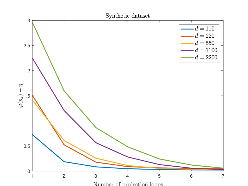
Figure 2: Convergence of the projection loop (7 iterations).

Remark 1 (multiple constraints)

We have presented above the case of a single constraint, since it is the setting employed in subsequent sections. However, the results of [10, Section 6.5] enable us to extend this approach to problems with $p$ constraints, see Appendix A.

III-C Application to Problem 1

It follows from (5), (26), and (27), that (31) for the classification problem can be written explicitly as follows, where $\varepsilon$ is an arbitrarily small number in $\left]0,1\right[$ and where $\beta$ is given by (6).

$$\begin{array}[]{l}\text{for}\;n=0,1,\ldots\\ \left\lfloor\hskip-2.84526pt\begin{array}[]{l}\gamma_{n}\in[\varepsilon,(2-\varepsilon)/\beta]\\ v_{n}=w_{n}-\dfrac{\gamma_{n}}{m}\displaystyle\sum_{i=1}^{m}\mathsf{y}_{i}\phi^{\prime}\big{(}\mathsf{y}_{i}{\left\langle{{x_{i}}\mid{w_{n}}}\right\rangle}\big{)}x_{i}\\[-2.84526pt] p_{0}=v_{n}\\ \begin{array}[]{l}\hskip-5.69054pt\text{for}\;k=0,1,\ldots,K_{n}-1\\ \hskip-2.84526pt\left\lfloor\hskip-2.84526pt\begin{array}[]{l}\zeta_{k}=\eta-\varphi(p_{k})\\ \text{if}\;\zeta_{k}\geqslant 0\\ \!\!\begin{array}[]{l}\left\lfloor\text{terminate.}\right.\\ \end{array}\\ s_{k}\in\partial\varphi(p_{k})\\ p_{k+1/2}=p_{k}+\zeta_{k}s_{k}/\|s_{k}\|^{2}\\ \chi_{k}={\left\langle{{p_{0}-p_{k}}\mid{p_{k}-p_{k+1/2}}}\right\rangle}\\ \mu_{k}=\|p_{0}-p_{k}\|^{2}\\ \nu_{k}=\|p_{k}-p_{k+1/2}\|^{2}\\ \rho_{k}=\mu_{k}\nu_{k}-\chi_{k}^{2}\\ \text{if}\;\rho_{k}=0\;\text{and}\;\chi_{k}\geqslant 0\\ \!\!\begin{array}[]{l}\left\lfloor p_{k+1}=p_{k+1/2}\right.\\[5.69054pt] \end{array}\\ \text{if}\;\rho_{k}>0\;\text{and}\;\chi_{k}\nu_{k}\geqslant\rho_{k}\\ \!\!\begin{array}[]{l}\left\lfloor p_{k+1}=\displaystyle p_{0}+\bigg{(}1+\frac{\chi_{k}}{\nu_{k}}\bigg{)}\big{(}p_{k+1/2}-p_{k}\big{)}\right.\\[5.69054pt] \end{array}\\[11.38109pt] \text{if}\;\rho_{k}>0\;\text{and}\;\chi_{k}\nu_{k}<\rho_{k}\\ \!\!\begin{array}[]{l}\left\lfloor\!\!\begin{array}[]{l}p_{k+1}\!=\!\displaystyle p_{k}\!+\!\frac{\nu_{k}}{\rho_{k}}\Big{(}\chi_{k}\big{(}p_{0}\!-\!p_{k}\big{)}\!+\!\mu_{k}\big{(}p_{k+1/2}\!-\!p_{k}\big{)}\Big{)}\end{array}\right.\\[5.69054pt] \end{array}\end{array}\right.\\[5.69054pt] \end{array}\\ w_{n+1}=p_{K_{n}}.\end{array}\right.\\[5.69054pt] \end{array}$$ (32)

A subgradient of $\varphi_{1}$ at $(\xi_{i})_{1\leqslant i\leqslant d}\in\mathbb{R}^{d}$ is $s=(\operatorname{sign}(\xi_{i}))_{1\leqslant i\leqslant d}$, where

$$\operatorname{sign}\colon\xi\mapsto\begin{cases}1&\text{if}\;\;\xi>0\\ 0&\text{if}\;\;\xi=0\\ -1&\text{if}\;\;\xi<0.\end{cases}$$ (33)

The $i$th component of a subgradient of $\varphi_{2}$ at $(\xi_{i})_{1\leqslant i\leqslant d}\in\mathbb{R}^{d}$ is given by

$$\sum_{(i,j)\in\mathsf{S}}\begin{cases}\operatorname{sign}(\xi_{i})&\text{if}\;\;|\xi_{i}|\geqslant|\xi_{j}|\\ 0&\text{otherwise}.\end{cases}$$ (34)

The $i$th component of a subgradient of $\varphi_{3}$ at $(\xi_{i})_{1\leqslant i\leqslant d}\in\mathbb{R}^{d}$ is given by

$$\sum_{(i,j)\in\mathsf{S}}\begin{cases}\operatorname{sign}(\xi_{i}-\xi_{j})&\text{if}\;\;\xi_{i}\neq\xi_{j}\\ 0&\text{otherwise}.\end{cases}$$ (35)

III-D Application to regression

A common approach in regression is to learn $w\in\mathbb{R}^{d}$ by employing the quadratic loss

$$\Psi\colon\mathbb{R}^{d}\to\mathbb{R}\colon w\mapsto\dfrac{1}{2m}\displaystyle\sum_{i=1}^{m}\big{|}{\left\langle{{x_{i}}\mid{w}}\right\rangle}-\mathsf{y}_{i}\big{|}^{2}$$ (36)

instead of the function $\Phi$ of (13) in Problem 2. Since $\Psi$ is convex and has a Lipschitz-continuous gradient with constant $\beta=\sigma_{1}^{2}$, where $\sigma_{1}$ is the largest singular value of the matrix $[x_{1}|\cdots|x_{m}]$, it suffices to change the definition of $v_{n}$ in (32) by

$$v_{n}=w_{n}-\dfrac{\gamma_{n}}{m}\displaystyle\sum_{i=1}^{m}({\left\langle{{x_{i}}\mid{w_{n}}}\right\rangle}-\mathsf{y}_{i}\big{)}x_{i}.$$ (37)

IV Experimental evaluation

We illustrate the performance of the proposed constrained splitting method on both synthetic and real data sets.

IV-A Synthetic data set

We first simulate a simple regulatory network in genomic described in [27]. A genomic network is composed of regulators (transcription factors, cytokines, kinase, growth factors, etc.) and the genes they regulate. Our notation is as follows:

• $m$: number of samples.

• $N_{\text{reg}}$: number of regulators.

• $N_{\text{g}}$: number of genes per regulator.

• $d=N_{\text{reg}}(N_{\text{g}}+1)$.

The entry $\xi_{i,j}$ of the matrix $X=[x_{1}|\cdots|x_{m}]^{\top}$, composed of $m$ rows and $d$ columns, is as follows.

1. The $r$th regulator of the $i$th sample is

   $$\xi_{i,\text{reg}_{r}}=\xi_{i,N_{\text{g}}(r-1)+r}=\xi_{i,r(N_{\text{g}}+1)-N_{\text{g}}}\sim\mathcal{N}(0,1).$$

   This defines $\xi_{i,j}$ for $j$ of the form $r(N_{\text{g}}+1)-N_{\text{g}}$.

2. The genes associated with $\xi_{i,\text{reg}_{r}}$ have a joint bivariate normal distribution with a correlation of $\rho=0.7$

   $$\xi_{i,r(N_{\text{g}}+1)-N_{\text{g}}+k}\sim\mathcal{N}\big{(}\varrho\,\xi_{i,\text{reg}_{r}},1-\varrho^{2}\big{)}.$$

   This defines $\xi_{i,j}\neq r(N_{\text{g}}+1)-N_{\text{g}}$.

The regression response $\mathsf{Y}$ is given by $\mathsf{Y}=Xw+\varepsilon$, where $\varepsilon\sim\mathcal{N}(0,\sigma^{2})$ with $\sigma=2$.

Example 1

In this example, we consider that $9$ genes regulated by the same regulators are activated and $1$ gene is inhibited. The true regressor is defined as

$$\begin{array}[]{l}w=\Bigg{(}5,\underbrace{\frac{5}{\sqrt{10}},\ldots}_{9},\underbrace{\frac{-5}{\sqrt{10}},\ldots}_{1},-5,\underbrace{\frac{-5}{\sqrt{10}},\ldots}_{9},\underbrace{\frac{5}{\sqrt{10}},\ldots}_{1},3,\\ \underbrace{\frac{3}{\sqrt{10}},\ldots}_{9},\underbrace{\frac{-3}{\sqrt{10}},\ldots}_{1},-3,\underbrace{\frac{-3}{\sqrt{10}},\ldots}_{9},\underbrace{\frac{3}{\sqrt{10}},\ldots}_{1},0,\ldots\!,0\Bigg{)}.\end{array}$$

Example 2

We consider that $8$ genes regulated by the same regulators are activated and $2$ genes are inhibited. The true regressor is defined as

$$\begin{array}[]{l}w=\Bigg{(}5,\underbrace{\frac{5}{\sqrt{10}},\ldots}_{8},\underbrace{\frac{-5}{\sqrt{10}},\ldots}_{2},-5,\underbrace{\frac{-5}{\sqrt{10}},\ldots}_{8},\underbrace{\frac{5}{\sqrt{10}},\ldots}_{2},3,\\ \underbrace{\frac{3}{\sqrt{10}},\ldots}_{8},\underbrace{\frac{-3}{\sqrt{10}},\ldots}_{2},-3,\underbrace{\frac{-3}{\sqrt{10}},\ldots}_{8},\underbrace{\frac{3}{\sqrt{10}},\ldots}_{2},0,\ldots\!,0\Bigg{)}.\end{array}$$

Example 3

This example is similar to Example 1, but we consider that $7$ genes regulated by the same regulators are activated and $3$ genes are inhibited. The true regressor is

$$\begin{array}[]{l}w=\Bigg{(}5,\underbrace{\frac{5}{\sqrt{10}},\ldots}_{7},\underbrace{\frac{-5}{\sqrt{10}},\ldots}_{3},-5,\underbrace{\frac{-5}{\sqrt{10}},\ldots}_{7},\underbrace{\frac{5}{\sqrt{10}},\ldots}_{3},3,\\ \underbrace{\frac{3}{\sqrt{10}},\ldots}_{7},\underbrace{\frac{-3}{\sqrt{10}},\ldots}_{3},-3,\underbrace{\frac{-3}{\sqrt{10}},\ldots}_{7},\underbrace{\frac{3}{\sqrt{10}},\ldots}_{3},0,\ldots\!,0\Bigg{)}.\end{array}$$

IV-B Breast cancer data set

We use the breast cancer data set [36], which consists of gene expression data for 8,141 genes in 295 breast cancer tumors (78 metastatic and 217 non-metastatic). In the time comparison evaluation, we select a subset of the 8141 genes (range 3000 to 7000) using a threshold on the mean of the genes. We use the network provided in [8] with $p=639$ pathways as graph constraints in our classifier. In biological applications, pathways are genes grouped according to their biological functions [8, 27]. Two genes are connected if they belong to the same pathway. Let $\mathsf{S_{i}}$ be the subset of genes that are connected to gene $i$. In this case, we have a subset of only 40,000 connected genes in $\mathsf{S_{i}}$. Note that we compute the subgradient (34) only on the subset $\mathsf{S_{i}}$ of connected genes.

IV-C Comparison between penalty method and our $\ell^{1}$ constrained method for classification

First, we compare with the penalty approach using glmnet MATLAB software [31] on the breast cancer data set described in Section IV-B. We tuned the number of path iterations $n_{\lambda}$ for glmnet for different values of the feature dimension. The number of nonzero coefficients $\|w\|_{0}$ increases with $n_{\lambda}$. The glmnet method requires typically 200 path iterations or more (see Fig. 3).

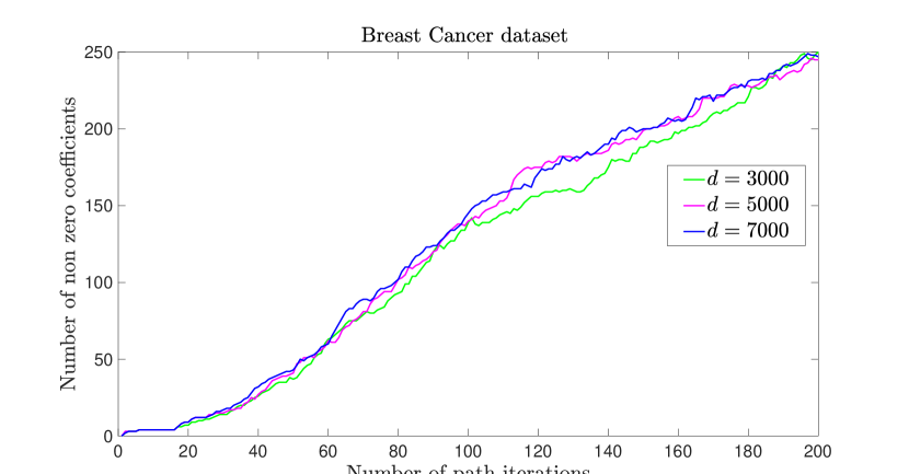
Figure 3: Glmnet: Number of nonzero coefficients as a function of $n_{\lambda}$.

Our classification implementation uses the logistic loss. Let $\|w\|_{1}\leqslant\eta$ be the surrogate sparsity constraint. Fig. 4 shows for different values of the feature dimension that the number of nonzero coefficients $\|w\|_{0}$ decreases monotonically with the number of iterations. Consequently, the sweep search over $\eta$ consists in stopping the iterations of the algorithm when $\|w\|_{0}$ reaches value specified a priori.

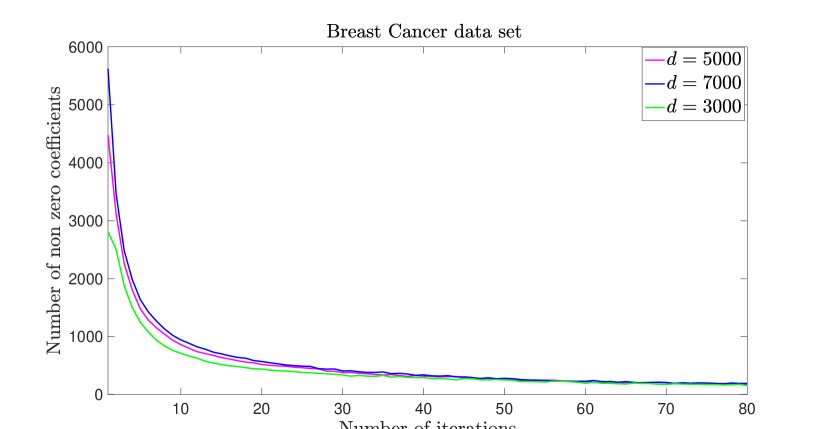
Figure 4: Number of nonzero coefficients as a function of the number of iterations.

Our direct constrained strategy does not require the often heuristic search for meaningful and interpretable Lagrange multipliers. Moreover, we can improve processing time using sparse computing. Namely, at each iteration we compute scalar products using only the sparse sub-vector of nonzero values. We compare time processing using the breast cancer data set ($n=295$ samples, $d=3022$) described in Section IV-B. We provide time comparison using a 2.5 GHz Macbook Pro with an i7 processor and Matlab software. We report time processing in Table I using glmnet software [31] and our method using either Matlab $\ell^{1}$ or a standard mex $\ell^{1}$ file. Moreover, since the vector $w$ is sparse, we provide mex-sparse and matlb-sparse times using sparse computing.

TABLE I: Time comparison (Matlab and mex) versus glmnet [31].

	mex-sparse	mex	Matlab	Matlab-sparse	mex [31]
Time(s)	0.0230	0.0559	0.169	0.0729	0.198

Fig. 5 shows that our constrained method is ten times faster than glmnet [31]. A numerical experiment is available in [1].

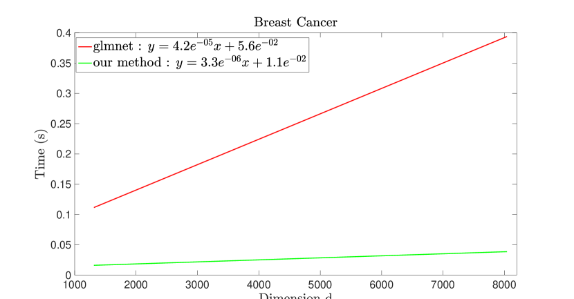
Figure 5: Computing time as a function of the dimension.

A potentially competitive alternative $\ell^{1}$ constrained optimization algorithms for solving the projection part of our constrained classification splitting algorithm is that described in [15]. We plug the specific projection onto the ball algorithm into our splitting algorithm. We provide time comparison (in seconds) in Table II for classification for the breast cancer data set ($d=3022$) described in Section IV-B.

TABLE II: Time comparison(s) with projection onto the ball [15] for dimension $d=3022$ using Matlab.

	Matlab	Matlab sparse	ball [15]
Time (s)	0.169	0.0729	0.149

Note that the most expensive part of our algorithm in terms of computation is the evaluation of the gradient. Although the projection onto the ball [15] is faster than our projection, our method is basically $12\%$ slower than the specific $\varphi_{1}$ constrained method for dimension $d=3022$. However, our sparse implementation of scalar products is twice as fast. Moreover, since the complexity of our method relies on the computation of scalar products, it can be easily speed up using multicore CPU or Graphics Processing Unit (GPU) devices, while the speed up of the projection on the ball [15] using CPU or GPU is currently an open issue. In addition our method is more flexible since it can take into account more sophisticated constraints such as $\varphi_{2}$, $\varphi_{3}$, or any convex constraint. We evaluate classification performance using area under the ROC curve (AUC). The result of Table III show that our $\varphi_{1}$ constrained method outperforms the $\varphi_{1}$ penalty method by $5.8\%$. Our $\varphi_{2}$ constraint improves slightly the AUC by $1\%$ over the $\varphi_{1}$ constrained method. We also observe a significant improvement of our constrained $\varphi_{2}$ method over the penalty group Lasso approach discussed in [24]. In addition, the main benefit of the $\varphi_{2}$ constraint is to provide a set of connected genes which is more relevant for biological analysis than the individual genes selected by the $\varphi_{1}$ constraint.

TABLE III: Breast cancer AUC comparisons.

	glmnet [31]	Group Lasso [24]	$\varphi_{1}$	$\varphi_{2}$
AUC ($\%$)	64.5	66.7	71.3	72.3

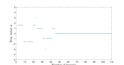
(a)

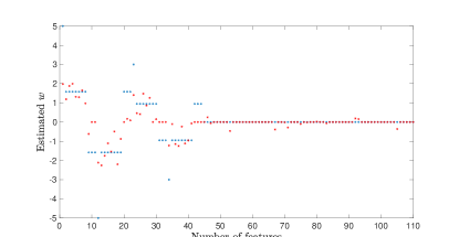
(b)

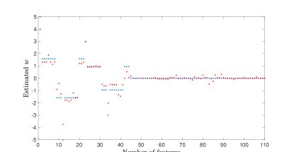
(c)

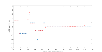
(d)

Figure 6: Example 3: (a): True vector $w$. (b): Estimation with the $\varphi_{1}$ constraint. (c): Estimation with the $\varphi_{2}$ constraint. (d): Estimation with the $\varphi_{4}$ constraint.

IV-D Comparison of various constraints for regression

In biological applications, gene activation or inhibition are well known and summarized in the ingenuity pathway analysis (IPA) database [2]. We introduce this biological a priori knowledge by replacing the $\varphi_{3}$ constraint by

$$\varphi_{4}\colon w\mapsto\sum_{(i,j)\in\mathsf{S}}{|\omega_{i}-a_{ij}\omega_{j}|},$$ (38)

where $a_{ij}=1$ if genes $i$ and $j$ are both activated or inhibited, and $a_{ij}=-1$ if gene $i$ is activated and gene $j$ inhibited. We compare the estimation of $w$ for Example 3 using $\varphi_{1}$ versus the $\varphi_{2}$ and $\varphi_{4}$ constraint. For each fold, we estimate the regression vector $w$ on $100$ training samples. Then we evaluate on new $100$ testing samples. We evaluate regression using the mean square error (MSE) in the training set and the predictive mean square error (PMSE) in the test set. We use randomly half of the data for training and half for testing, and then we average the accuracy over 50 random folds.

We show in Fig. 6a the true regression vector and, in Fig. 6b, the estimation using the $\varphi_{1}$ constraint for Example 3. In Fig. 6c we show the results of the estimation with the $\varphi_{2}$ constraint, and in Fig. 6d with the $\varphi_{4}$ constraint. We provide for the three examples the mean square error as a function of $\eta$ for $\varphi_{1}$ (Fig. 7), $\varphi_{2}$ (Fig. 8), and $\varphi_{4}$ (Fig. 9).

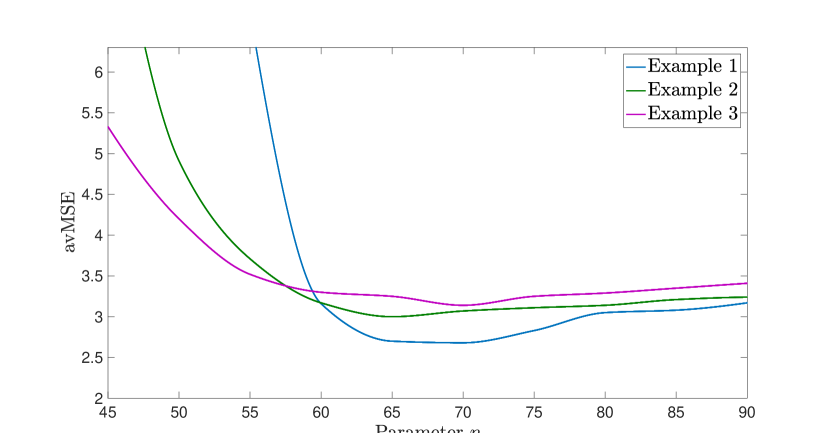
Figure 7: $\varphi_{1}$ constraint for Examples 1, 2, and 3. Mean square error as a function of the parameter $\eta$.

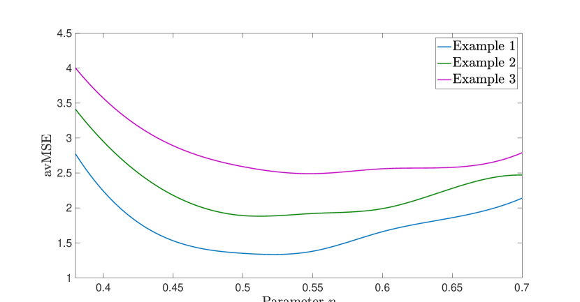
Figure 8: $\varphi_{2}$ constraint for Examples 1, 2, and 3. Mean square error as a function of the parameter $\eta$.

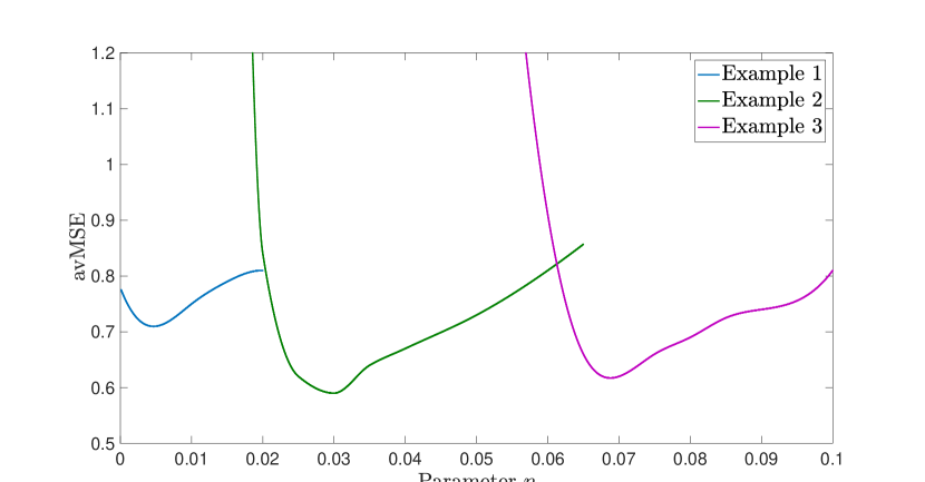
Figure 9: $\varphi_{4}$ constraint for Examples 1, 2, and 3. Mean square error as a function of the parameter $\eta$.

We report for Example 2 in Fig. 10 the estimation of the mean square error in the training set as a function of the number of training samples for the $\varphi_{1}$, $\varphi_{2}$, and $\varphi_{4}$ constraint.

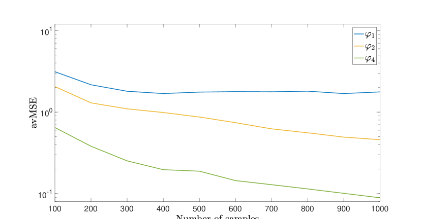
Figure 10: MSE as a function of the number of samples $m$ for Example 2.

The $\varphi_{4}$ constraint outperforms both the $\varphi_{2}$ and the $\varphi_{1}$ constrained method. However, the selection of the parameter $\eta$ for constraint $\varphi_{4}$ is more challenging.

V Conclusion

We have used constrained optimization approaches to promote sparsity and feature grouping in classification and regression problems. To solve these problems, we have proposed a new efficient algorithm which alternates a gradient step on the data fidelity term and an approximate projection step onto the constraint set. We have also discussed the generalization to multiple constraints. Experiments on both synthetic and biological data show that our constrained approach outperforms penalty methods. Moreover, the formulation using the $\varphi_{4}$ constraint outperforms those using the pairwise $\varphi_{2}$ and the $\varphi_{1}$ constraint.

Appendix A – The case of multiple constraints

Let $\Phi$ be as in Problem 2 and, for every $j\in\{1,\ldots,p\}$, let $\varphi_{j}\colon\mathbb{R}^{d}\to\mathbb{R}$ be convex, let $\eta_{j}\in\mathbb{R}$, and let $\omega_{j}\in\left]0,1\right]$ be such that $\sum_{j=1}^{p}\omega_{j}=1$. Consider the problem

$$\underset{\begin{subarray}{c}{\begin{subarray}{c}\varphi_{1}(w)\leqslant\eta_{1}\\[-2.84526pt] ~{}~{}~{}~{}\vdots\\[2.84526pt] \varphi_{p}(w)\leqslant\eta_{p}\end{subarray}}\end{subarray}}{\text{\rm minimize}}\;\;\Phi(w).$$ (A1)

In other words, $C=\bigcap_{j=1}^{p}\big{\{}{w\in\mathbb{R}^{d}}~{}\big{|}~{}{\varphi_{j}(w)\leqslant\eta_{j}}\big{\}}$ in (16). Let $k\in\mathbb{N}$. For every $j\in\{1,\ldots,p\}$, let $s_{j,k}\in\partial\varphi_{j}(p_{k})$ and set

$$p_{j,k}=\begin{cases}p_{k}+\displaystyle{\frac{\eta_{j}-\varphi_{j}(p_{k})}{\|s_{j,k}\|^{2}}}s_{j,k}&\text{if}\;\;\varphi_{j}(p_{k})>\eta_{j}\\ p_{k}&\text{if}\;\;\varphi_{j}(p_{k})\leqslant\eta_{j}.\end{cases}$$ (A2)

Now define

$$p_{k+1/2}=p_{k}+L_{k}\Bigg{(}\displaystyle\sum_{j=1}^{p}\omega_{j}p_{j,k}-p_{k}\Bigg{)},$$ (A3)

where

$$L_{k}=\frac{\displaystyle\sum_{j=1}^{p}\omega_{j}\|p_{j,k}-p_{k}\|^{2}}{\Bigg{\|}\displaystyle\sum_{j=1}^{p}\omega_{j}p_{j,k}-p_{k}\Bigg{\|}^{2}}.$$ (A4)

Then $p_{k+1}=Q(p_{0},p_{k},p_{k+1/2})\to P_{C}(p_{0})$ [10, Theorem 6.4] and therefore the generalization

$$\begin{array}[]{l}\text{for}\;n=0,1,\ldots\\ \left\lfloor\begin{array}[]{l}v_{n}=w_{n}-\gamma_{n}\nabla\Phi(w_{n})\\ p_{0}=v_{n}\\ \begin{array}[]{l}\hskip-5.69054pt\text{for}\;k=0,1,\ldots,K_{n}-1\\ \left\lfloor\begin{array}[]{l}\zeta_{k}=\min_{1\leqslant j\leqslant p}\big{(}\eta_{j}-\varphi_{j}(p_{k})\big{)}\\ \text{if}\;\zeta_{k}\geqslant 0\\ \begin{array}[]{l}\left\lfloor\text{terminate.}\right.\\ \end{array}\\ \text{for}\;j=1,\ldots,p\\ \begin{array}[]{l}\left\lfloor s_{j,k}\in\partial\varphi_{j}(p_{k})\right.\\ \end{array}\\ \text{compute}\>p_{k+1/2}\;\text{as in \eqref{e:e-radigue0}--\eqref{e:e-radigue2}}\end{array}\right.\\[5.69054pt] \end{array}\\ w_{n+1}=p_{K_{n}}.\end{array}\right.\\[5.69054pt] \end{array}$$ (A5)

of (31) solves (A1).

References

- [1] http://www.i3s.unice.fr/~barlaud/code.html
- [2] http://www.ingenuity.com/products/ipal
- [3] H. H. Bauschke and P. L. Combettes, Convex Analysis and Monotone Operator Theory in Hilbert Spaces, 2nd ed. Springer, New York, 2017.
- [4] W. Belhajali, R. Nock, and M. Barlaud, “Boosting stochastic Newton with entropy constraint for large-scale image classification,” in Proc. 22nd Int. Conf. Pattern Recognit. (ICPR-14), 2014, pp. 232–237.
- [5] H. D. Bondell and B. J. Reich, “Simultaneous regression shrinkage, variable selection, and supervised clustering of predictors with OSCAR,” Biometrics, vol. 64, pp. 115–123, 2008.
- [6] E. J. Candès, “The restricted isometry property and its implications for compressed sensing,” C. R. Acad. Sci. Paris Sér. I, vol. 346, pp. 589–592, 2008.
- [7] Y. Censor and A. Lent, “Cyclic subgradient projections,” Math. Programming, vol. 24, pp. 233–235, 1982.
- [8] H.-Y. Chuang, E. Lee, Y.-T. Liu, D. Lee, and T. Ideker, “Network-based classification of breast cancer metastasis,” Mol. Syst. Biol., vol. 3, pp. 1175–1182, 2007.
- [9] P. L. Combettes, “Convex set theoretic image recovery by extrapolated iterations of parallel subgradient projections," IEEE Trans. Image Processing, vol. 6, pp. 493–506, 1997.
- [10] P. L. Combettes, “Strong convergence of block-iterative outer approximation methods for convex optimization,” SIAM J. Control Optim., vol. 38, pp. 538–565, 2000.
- [11] P. L. Combettes and J. C. Pesquet, “Image restoration subject to a total variation constraint," IEEE Trans. Image Process., vol. 13, pp. 1213–1222, 2004.
- [12] P. L. Combettes and J.-C. Pesquet, “Proximal thresholding algorithm for minimization over orthonormal bases,” SIAM J. Optim., vol. 18, pp. 1351-1376, 2007.
- [13] P. L. Combettes and J.-C. Pesquet, “Proximal splitting methods in signal processing,” in Fixed-Point Algorithms for Inverse Problems in Science and Engineering. Springer, 2011, pp. 185–212.
- [14] P. L. Combettes and V. R. Wajs, “Signal recovery by proximal forward-backward splitting,” Multiscale Model. Simul., vol. 4, pp. 1168–1200, 2005.
- [15] L. Condat, “Fast projection onto the simplex and the ball,” Math. Programming, vol. A158, pp. 575–585, 2016.
- [16] I. Daubechies, R. DeVore, M. Fornasier, and C. S. Güntürk, “Iteratively reweighted least squares minimization for sparse recovery,” Comm. Pure Appl. Math., vol. 63, pp. 1–38, 2010.
- [17] D. L. Donoho and M. Elad, “Optimally sparse representation in general (nonorthogonal) dictionaries via minimization,” Proc. Natl. Acad. Sci. USA, vol. 100, pp. 2197–2202, 2003.
- [18] D. L. Donoho and B. F. Logan, “Signal recovery and the large sieve,” SIAM J. Appl. Math., vol. 52, pp. 577–591, 1992.
- [19] D. L. Donoho and P. B. Stark, “Uncertainty principles and signal recovery,” SIAM J. Appl. Math., vol. 49, pp. 906–931, 1989.
- [20] M. A. T. Figueiredo and R. D. Nowak, “Ordered weighted regularized regression with strongly correlated covariates: Theoretical aspects,” Proc. 19th Int. Conf. Artif. Intell. Stat. (AISTATS), Cadiz, Spain, 2016.
- [21] J. Friedman, T. Hastie, and R. Tibshirani, “Regularization paths for generalized linear models via coordinate descent,” J. Stat. Software, vol. 33, pp. 1–22, 2010.
- [22] T. Hastie, S. Rosset, R. Tibshirani, and J. Zhu, “The entire regularization path for the support vector machine,” J. Mach. Learn. Res., vol. 5, pp. 1391–1415, 2004.
- [23] Y. Haugazeau, Sur les Inéquations Variationnelles et la Minimisation de Fonctionnelles Convexes. Thèse de doctorat, Université de Paris, 1968.
- [24] L. Jacob, G. Obozinski, and J.-P. Vert, “Group lasso with overlap and graph lasso,” in Proc. 26th Int. Conf. Mach. Learn. (ICML-09), 2009, pp. 353–360.
- [25] E. S. Levitin and B. T. Polyak, “Constrained minimization methods," USSR Comput. Math. Math. Phys., vol. 6, pp. 1–50, 1966.
- [26] A. S. Lewis and J.-S. Pang, “Error bounds for convex inequality systems,” in Generalized Convexity, Generalized Monotonicity: Recent Results. Springer, 1998, pp. 75–110.
- [27] C. Li and H. Li, “Network-constrained regularization and variable selection for analysis of genomic data,” Bioinformatics, vol. 24, pp. 1175–1182, 2008.
- [28] J. Mairal and B. Yu, “Complexity analysis of the lasso regularization path,” in Proc. 29th Int. Conf. Mach. Learn. (ICML-12), 2012, pp. 353–360.
- [29] K. Matusita, “Distance and decision rules,” Ann. Inst. Statist. Math., vol. 16, pp. 305–315, 1964.
- [30] S. Mosci, L. Rosasco, M. Santoro, A. Verri, and S. Villa, “Solving structured sparsity regularization with proximal methods,”in Machine Learning and Knowledge Discovery in Databases. Springer, 2010, pp. 418–433.
- [31] J. Qian, T. Hastie, J. Friedman, R. Tibshirani, and N. Simon, “Glmnet for matlab,” http://web.stanford.edu/~hastie/glmnet_matlab/, 2013.
- [32] M. Schmidt, N. L. Roux, and F. R. Bach, “Convergence rates of inexact proximal-gradient methods for convex optimization,” in Advances in Neural Information Processing Systems, 2011, pp. 1458–1466.
- [33] S. Sra, S. Nowozin, and S. J. Wright, Optimization for Machine Learning. MIT Press, Cambridge, MA, 2012.
- [34] R. Tibshirani, Regression shrinkage and selection via the lasso, J. Roy. Stat. Soc., vol. B58, pp. 267–288, 1996.
- [35] R. Tibshirani, M. Saunders, S. Rosset, J. Zhu, and K. Knight, “Sparsity and smoothness via the fused lasso,” J. Roy. Stat. Soc., vol. B67, pp. 91–108, 2005.
- [36] M. J. van De Vijver et al., “A gene-expression signature as a predictor of survival in breast cancer,” New Engl. J. Med., vol. 347, pp. 1999–2009, 2002.