On the robustness of the $q$–Gaussian family

Abstract

We introduce three deformations, called $\alpha$–, $\beta$– and $\gamma$–deformation respectively, of a $N$–body probabilistic model, first proposed by Rodríguez et al. (2008), having $q$–Gaussians as $N\to\infty$ limiting probability distributions. The proposed $\alpha$– and $\beta$–deformations are asymptotically scale–invariant, whereas the $\gamma$–deformation is not. We prove that, for both $\alpha$– and $\beta$–deformations, the resulting deformed triangles still have $q$–Gaussians as limiting distributions, with a value of $q$ independent (dependent) on the deformation parameter in the $\alpha$–case ($\beta$–case). In contrast, the $\gamma$–case, where we have used the celebrated $Q$–numbers and the Gauss binomial coefficients, yields other limiting probability distribution functions, outside the $q$–Gaussian family. These results suggest that scale–invariance might play an important role regarding the robustness of the $q$–Gaussian family.

I Introduction

It is well known that the (properly centered and rescaled) sum of $N$ independent (or weakly dependent) random variables with finite variance approaches a Gaussian distribution in the $N\to\infty$ limit Feller (1971). This fundamental classical result, known as the Central Limit Theorem (CLT), is at the basis of the ubiquity of Gaussian distributions in Nature. The classical CLT, however, cannot be applied to a set of strongly correlated random variables. Therefore, in the context of nonextensive statistical mechanics Tsallis (2009a), it has been argued the existence of a generalized CLT for random variables correlated in a specific way Umarov et al. (2008, 2010), called $q$–independence. Alternative CLTs, based on a different kind of correlations Vignat and Plastino (2007) or on exchangeability Hahn et al. (2010), have also been proposed in the literature. In all these theorems, the (properly centered and rescaled) sum of $N$ correlated random variable has, in the $N\to\infty$ limit, a $q$–Gaussian distribution $P_{q}(x)$,

$$P_{q}(x)\coloneqq\begin{cases}\sqrt{\frac{q-1}{\pi}}\frac{\Gamma\left(\frac{1}{q-1}\right)}{\Gamma\left(\frac{3-q}{2q-2}\right)}e_{q}^{-x^{2}}&q\in(1,3),\\ \frac{1}{\sqrt{\pi}}e^{-x^{2}}&q=1,\\ \sqrt{\frac{1-q}{\pi}}\frac{3-q}{2}\frac{\Gamma\left(\frac{3-q}{2-2q}\right)}{\Gamma\left(\frac{1}{1-q}\right)}e_{q}^{-x^{2}}&q\in(-\infty,1),\end{cases}$$ (1)

where $q$ is a real parameter depending on the nature of the correlations, and the $q$–exponential function is defined as follows:

$$e_{q}^{x}\coloneqq\begin{cases}e^{x}&q=1,\\ \left[1+(1-q)x\right]_{+}^{\frac{1}{1-q}}&q\neq 1,\end{cases}$$ (2)

with $[x]_{+}\coloneqq x\,\theta(x)$, $\theta(x)$ Heaviside function. In what follows, we will use also the inverse function of the $q$–exponential, the $q$–logarithm, defined as

$$\log_{q}(x)\coloneqq\begin{cases}\ln(x)&q=1,\\ \frac{x^{1-q}-1}{1-q}&q\neq 1,\end{cases}\qquad x>0.$$ (3)

Like Gaussian distributions, $q$–Gaussians also are ubiquitous in Nature. Indeed, analytical, experimental and numerical investigations in biology Upadhyaya et al. (2001), economics Tsallis et al. (2003); Borland (2002), high energy physics Wong and Wilk (2013), anomalous diffusion processes Tsallis and Bukman (1996); Andrade Jr et al. (2010), dynamics of many-body classical Hamiltonian systems Anteneodo and Tsallis (1998); Leo et al. (2012); Cirto et al. (2014); Pluchino et al. (2007), cold atoms Douglas et al. (2006); Lutz (2003); Lutz and Renzoni (2013), dissipative and conservative low dimensional maps Tirnakli et al. (2007); Tirnakli and Borges (2015), turbulence Boghosian (1996) among others, have shown that $q$–Gaussian distributions appear in the probabilistic analysis of many systems in which long–range interactions are present, or ergodicity lacks. These evidences strongly support the existence of a generalized CLT involving $q$–Gaussians.

To investigate the conditions under which such a generalized CLT holds, analytically solvable probabilistic models yielding $q$–Gaussian limiting distributions are of paramount importance. In particular, in Rodríguez et al. (2008) a probabilistic model for $N$ correlated binary random variables was introduced, generalizing the celebrated Leibniz triangle Polya (1962). The proposed model preserves the scale–invariance property (see Ref. Rodríguez et al. (2008) and below for a definition) of the Leibniz triangle and it can be rigorously proved that this model has $q$–Gaussians with $q\in[0,1]$ as limiting distributions for $N\to\infty$. Subsequently, it was shown Rodríguez and Tsallis (2012, 2014) that particular $d$–dimensional scale–invariant probabilistic models with $d\geq 1$ have, as limiting distributions, Dirichlet distributions for $d>1$, whereas for $d=1$ $q$–Gaussians were obtained. The ultimate relationship between scale–invariance and $q$–Gaussianity, i.e. the appearance of $q$–Gaussians as probability distributions for statistical models in the thermodynamic limit, is not yet completely clear. In Refs. Rodríguez et al. (2008); Tsallis et al. (2005) it was already conjectured that (asymptotic) scale invariance could be possibly a necessary but not sufficient condition, for the emergence of $q$-Gaussians. Indeed, in Hilhorst and Schehr (2007) two scale–invariant probabilistic models which are different from the one analyzed here, are analytically studied, showing a limiting distribution different from a $q$–Gaussian.

With the aim of shedding further light on this problem, we address here the robustness under small perturbations of the general one–parameter family of scale–invariant probabilistic models introduced in Rodríguez et al. (2008). In particular, we investigate the stability of the $q$–Gaussian family in the space of probability distributions: this property is indeed fundamental for the existence of a generalized CLT yielding $q$–Gaussian distributions in Nature. In this context, exactly solvable probabilistic models are essential tools for a rigorous study of the type of correlations and the properties required for such generalized theorem.

We consider two new families of asymptotically scale–invariant triangles, namely the $\alpha$–triangles and $\beta$–triangles, which generalize the aforementioned family. These deformations are based on the introduction of two classes of real numbers, the $\alpha$–numbers and $\beta$–numbers respectively, in the same spirit of the $Q$–numbers, typical of the $Q$–deformations of Lie groups and algebras Kac and Cheung (2002). As we shall see, despite the deformation, the limiting distributions remain $q$–Gaussians, but with a value of $q$ which might depend on the perturbation strength.

To the best of our knowledge, this is the first article addressing, for specific probabilistic models, the important problem of the robustness of $q$–Gaussians as attractors, a fundamental property involved in the existence of a generalized CLT.

The aforementioned deformations may be considered as nontrivial ones, since there is no a priori guarantee that an arbitrary deformation should preserve the same $q$–Gaussian behavior for large values of $N$. As a counterexample, we introduce and study here an alternative deformation, that we call $\gamma$–deformation, based on the classical definition of $Q$–number Kac and Cheung (2002) used in combinatorics. This deformation does not generically preserve $q$–Gaussian forms for the limiting distributions. Since scale–invariance is violated by the $\gamma$–deformation, in contrast with the $\alpha$– and $\beta$– ones, a possible conjecture might emerge on the necessity of (at least asymptotic) scale-invariance for $q$–Gaussianity (see also Tsallis et al. (2005)).

II Preliminaries: Leibniz-like triangles as probability models

Let us consider a system with $N$ identical elements, whose states are characterized by binary variables $x_{i}\in\{0,1\}$, $i=1,\,\dots,N$. Let us introduce also the probability $r_{N,n}$ of having a given configuration $\{x_{1},\dots,x_{N}\}$ with $\sum_{i=1}^{N}x_{i}=n$. The probability $p_{N,n}$ of having any configuration such that $\sum_{i=1}^{N}x_{i}=n$ is obtained taking into account the proper degeneracy

$$p_{N,n}\coloneqq\binom{N}{n}r_{N,n}.$$ (4)

The set of values $r_{N,n}$ can be organized in a triangle, in such a way that the element $r_{N,n}$ is the $n$th element of the $N$th row. We require that the following Leibniz triangle rule (or scale–invariance property) holds:

$$r_{N,n+1}+r_{N,n}=r_{N-1,n}.$$ (5)

The Leibniz triangle $r^{(1)}_{N,n}$ Polya (1962) can be constructed using the Leibniz rule and defining $r_{N,0}^{(1)}$ as follows:

$$r^{(1)}_{N,0}\coloneqq\frac{1}{N+1}\Rightarrow r^{(1)}_{N,n}=\frac{1}{\binom{N}{n}}\frac{1}{N+1}.$$ (6)

The $N\to\infty$ limiting distribution is the uniform distribution. Considering instead $r_{N,0}=p^{N}$, $p\in(0,1)$, the $N\to\infty$ limiting distribution is a Gaussian distribution, being in this case $p_{N,n}=\binom{N}{n}p^{n}(1-p)^{N-n}$, i.e., the binomial distribution.

The aforementioned Leibniz triangle has been generalized in Rodríguez et al. (2008): for $\nu\in\mathds{N}$,

$$r^{(\nu)}_{N,0}\coloneqq\frac{\Gamma(2\nu)\Gamma(N+\nu)}{\Gamma(\nu)\Gamma(N+2\nu)}\Rightarrow r^{(\nu)}_{N,n}=\frac{r^{(1)}_{N+2(\nu-1),n+\nu-1}}{r^{(1)}_{2(\nu-1),\nu-1}}.$$ (7)

The triangle (6) is recovered as the $\nu=1$ particular case. Remarkably, it has been proved Rodríguez et al. (2008) that, for $N\to\infty$ and $\nu=2,3,\dots$, we have

$$p^{(\nu)}_{N,n}\coloneqq\binom{N}{n}r^{(\nu)}_{N,n}\mathbin{\overset{N\gg 1}{\kern 0.0pt\leavevmode\resizebox{22.44292pt}{3.66875pt}{$\sim$}}}\frac{2\sqrt{\nu-1}}{N}P_{q_{1}(\nu)}(x),\\ x\coloneqq 2\sqrt{\nu-1}\left(\frac{n}{N}-\frac{1}{2}\right),$$ (8)

where $P_{q_{1}(\nu)}(x)$ is a $q$–Gaussian with $q\equiv q_{1}(\nu)$,

$$q_{1}(\nu)=1-\frac{1}{\nu-1}<1\,;$$ (9)

the subindex 1 will become transparent later on. In the $\nu\to\infty$ limit, $r^{(\nu)}_{N,0}\to 2^{-N}$ and $q_{1}(\nu)\to 1$ as expected from the CLT.

III Asymptotically scale–invariant deformations of the generalized Leibniz triangle

In this Section, we introduce two asymptotically scale–invariant deformations of the probabilistic model analyzed in Rodríguez et al. (2008).

III.1 The $\alpha$–numbers and the $\alpha$–triangles

The basis of our construction is the notion of $\alpha$–number.

Definition III.1.

Given $n\in\mathds{N}\cup{0}$, and $\alpha>0$, $\alpha\neq 1$, an $\alpha$–number is the real number defined as follows:

$$\{n\}_{\alpha}\coloneqq(n+1)\left(1-\frac{1-\alpha}{1-{\alpha}^{n+1}}\right)=\begin{cases}na_{n}(\alpha)&n\geq 1\,,\\ 0&n=0\,,\end{cases}$$ (10)

where we have introduced ($n\geq 1$)

$$a_{n}(\alpha)\coloneqq\frac{n+1}{n}\left(1-\frac{1-\alpha}{1-{\alpha}^{n+1}}\right)\xrightarrow{\alpha\to 1}1\,.$$ (11)

The previous definition is such that

$$\{n\}_{1}\equiv\lim_{\alpha\to 1}\{n\}_{\alpha}=n\,,$$ (12)

so in the $\alpha\to 1$ limit we recover the ordinary numbers.

The following is a generalization of the factorial of a natural number.

Definition III.2.

Given $n\in\mathds{N}\cup 0$, we shall call $\alpha$–factorial the number defined as

$$\{0\}_{\alpha}!\coloneqq 1\text{ and }\{n\}_{\alpha}!\coloneqq\prod_{k=1}^{n}\{k\}_{\alpha}=n!\prod_{k=1}^{n}a_{k}(\alpha),\ n\in\mathds{N}.$$ (13)

The ordinary factorial is recovered in the $\alpha\to 1$ limit, $\{n\}_{1}!\equiv\lim_{\alpha\to 1}\{n\}_{\alpha}!=n!$. We define now an extension of the binomial coefficients.

Definition III.3.

Given the nonnegative integers $N$ and $n\leq N$, the $\alpha$–binomial coefficient is defined as

$$\left\{\begin{matrix}N\\ n\end{matrix}\right\}_{\alpha}\coloneqq\frac{\{N\}_{\alpha}!}{\{n\}_{\alpha}!\{N-n\}_{\alpha}!}\\ =\begin{cases}1&\text{if $n=0$ or $n=N$},\\ \binom{N}{n}\prod_{k=1}^{N-n}\frac{a_{k+n}(\alpha)}{a_{k}(\alpha)}&1\leq n\leq N-1.\end{cases}$$ (14)

The $\alpha$–binomial coefficients share with the Pascal coefficients the property $\left\{\begin{smallmatrix}N\\ n\end{smallmatrix}\right\}_{\alpha}=\left\{\begin{smallmatrix}N\\ N-n\end{smallmatrix}\right\}_{\alpha}$, $\forall\alpha$. Again, we recover the ordinary binomial coefficients in the $\alpha\to 1$ limit. In the same fashion as the Pascal triangle, the $\alpha$–binomial coefficients can be displayed forming a Pascal $\alpha$–triangle:

Deformation of the Leibniz–like triangles using the $\alpha$–numbers

We want now to deform the family of triangles obtained in Rodríguez et al. (2008) using the aforementioned $\alpha$–numbers. Let us start introducing the Leibniz–like $\alpha$–triangle as

$$r^{(1)}_{N,n,\alpha}\coloneqq\frac{1}{\{N+1\}_{\alpha}\left\{\begin{smallmatrix}N\\ n\end{smallmatrix}\right\}_{\alpha}},\quad n=0,\dots,N,$$ (15)

which is related to the original Leibniz triangle as

$$r^{(1)}_{N,n,\alpha}=\mu^{(1)}_{N,n,\alpha}r^{(1)}_{N,n},$$ (16)

with

$$\mu^{(1)}_{N,n,\alpha}\coloneqq\\ \begin{cases}1&\text{for $N=0$,}\\ \dfrac{1}{a_{N+1}(\alpha)}&\text{for $N>0$ and $n=0$ or $n=N$,}\\ \displaystyle\frac{\prod_{k=1}^{N-n}\frac{a_{k}(\alpha)}{a_{k+n}(\alpha)}}{a_{N+1}(\alpha)}&\text{for $N>0$ and $n=1,\dots,N-1$}.\end{cases}$$ (17)

In addition, $\lim_{\alpha\to 1}\mu^{(1)}_{N,n,\alpha}=1$. As an illustration, the $\alpha=\frac{1}{2}$ instance of family (15) is given by

The product of the Leibniz $\alpha$–triangle by the Pascal triangle (which takes into account the degeneracies) does not generically yield a set of probabilities, since

$$\sum_{n=0}^{N}\binom{N}{n}r^{(1)}_{N,n,\alpha}\neq 1.$$

Nevertheless we can circumvent this difficulty by properly renormalizing the triangle to get a new one with coefficients

$$\hat{r}^{(1)}_{N,n,\alpha}\coloneqq\dfrac{r^{(1)}_{N,n,\alpha}}{\sum_{k=0}^{N}\binom{N}{k}r^{(1)}_{N,k,\alpha}},$$ (18)

and associated probabilities

$$\hat{p}^{(1)}_{N,n,\alpha}\coloneqq\binom{N}{n}\hat{r}^{(1)}_{N,n,\alpha}.$$ (19)

The normalized Leibniz $\alpha$–triangle for $\alpha=\frac{1}{2}$ looks like

Following Ref. Rodríguez et al. (2008), we can define a two–parametric family of triangles from the Leibniz $\alpha$–triangle (15) for $\alpha>0$ and $\nu\in\mathds{N}$:

$$r^{(\nu)}_{N,n,\alpha}\coloneqq\frac{r^{(1)}_{N+2(\nu-1),n+\nu-1,\alpha}}{r^{(1)}_{2(\nu-1),\nu-1,\alpha}}=\mu^{(\nu)}_{N,n,\alpha}r^{(\nu)}_{N,n},$$ (20)

where, for $\nu>1$, we have

$$\mu^{(\nu)}_{N,n,\alpha}\coloneqq\\ \frac{a_{2\nu-1}(\alpha)}{a_{N+2\nu-1}(\alpha)}\prod_{k=1}^{N-n+\nu-1}\frac{a_{k}(\alpha)}{a_{k+n+\nu-1}(\alpha)}\prod_{k=1}^{\nu-1}\frac{a_{k+\nu-1}(\alpha)}{a_{k}(\alpha)}\\ =\frac{a_{2\nu-1}(\alpha)(\alpha-1)\left(\alpha^{N+2\nu}-1\right)}{\alpha(\alpha^{N-n+\nu}-1)(\alpha^{n+\nu}-1)}\cdot\\ \cdot\frac{(N-n+\nu)(n+\nu)}{N+2\nu}\prod_{k=1}^{\nu-1}\frac{a_{k+\nu-1}(\alpha)}{a_{k}(\alpha)}.$$ (22)

As before, normalization is needed to obtain the family

$$\hat{r}_{N,n,\alpha}^{(\nu)}\coloneqq\frac{r_{N,n,\alpha}^{(\nu)}}{\sum_{k=0}^{N}\binom{N}{k}r_{N,k,\alpha}^{(\nu)}},$$ (23)

with associated probabilities

$$\hat{p}_{N,n,\alpha}^{(\nu)}\coloneqq\binom{N}{n}\hat{r}_{N,n,\alpha}^{(\nu)}$$ (24)

trivially satisfying $\sum_{n=0}^{N}\hat{p}_{N,n,\alpha}^{(\nu)}=1$.

Observe that triangle (23) does not generically fulfill the scale–invariance condition (5). Nevertheless, it is asymptotically scale–invariant, i.e.,

$$\lim_{\begin{subarray}{c}N\to\infty\\ \frac{n}{N}\equiv\eta\text{ fixed}\end{subarray}}\frac{\hat{r}^{(\nu)}_{N-1,n,\alpha}}{\hat{r}^{(\nu)}_{N,n,\alpha}+\hat{r}^{(\nu)}_{N,n+1,\alpha}}=1.$$ (25)

This follows from the fact that the normalization $\sum_{n=0}^{N}\binom{N}{n}r_{N,n,\alpha}^{(\nu)}$ has a power–law scaling behavior (as we will see later by evaluating $\binom{N}{n}r^{(\nu)}_{N,n,\beta}$ for large $N$), and from the limit

$$\frac{r^{(1)}_{N-1+2(\nu-1),n+\nu-1,\alpha}}{r^{(1)}_{N+2(\nu-1),n+\nu-1,\alpha}+r^{(1)}_{N+2(\nu-1),n+\nu,\alpha}}\xrightarrow{N\to\infty}1,$$ (26)

obtained using the limit $a_{N}\xrightarrow{N\to\infty}\min\{1,\alpha\}$.

A theorem on the robustness of Leibniz–like $\alpha$–triangles

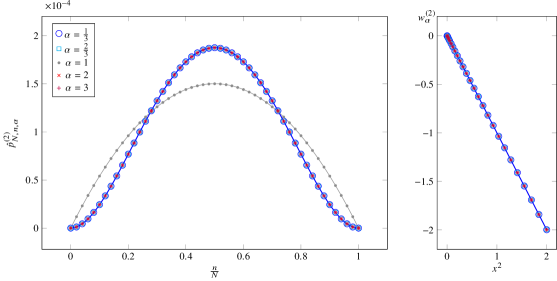
Figure 1: Probability distributions (24) and $w^{(\nu)}_{\alpha}(x)\coloneqq\log_{q_{\alpha}(\nu)}\frac{P_{q_{\alpha}(\nu)}(x)}{P_{q_{\alpha}(\nu)}(0)}$ for $\nu=2$, $N=10^{4}$ and different values of $\alpha$; the derived asymptotic behavior is also depicted as continuous line for $\alpha\neq 1$. The corresponding values of $q_{\alpha}(2)$ are given by Eq. (29).

In this Section, we prove that the family of deformed triangles (23) still possesses a $q$–Gaussian as limiting distribution for $N\rightarrow\infty$, after proper centering and rescaling. However, the limiting value of $q$ is different from $q_{1}(\nu)$, although not dependent on $\alpha$.

Theorem III.1.

The family of triangles (20) with $\nu\in(1,+\infty)$ and $\alpha\in\mathds{R}^{+}\setminus\{0\}$ satisfies the property

$$\frac{N}{2\sqrt{\nu-\delta_{\alpha,1}}}\hat{p}_{N,n,\alpha}^{(\nu)}\mathbin{\overset{N\gg 1}{\kern 0.0pt\leavevmode\resizebox{22.44292pt}{3.66875pt}{$\sim$}}}P_{q_{\alpha}(\nu)}(x),$$ (27)

where we have introduced the properly centered and rescaled variable

$$x\coloneqq 2\sqrt{\nu-\delta_{\alpha,1}}\left(\frac{n}{N}-\frac{1}{2}\right).$$ (28)

In Eq. (27), $P_{q_{\alpha}(\nu)}(x)$ is a $q$–Gaussian with

$$q_{\alpha}(\nu)\coloneqq 1-\frac{1}{\nu-\delta_{\alpha,1}}=\begin{cases}1-\frac{1}{\nu}&\text{for $\alpha\neq 1$},\\ 1-\frac{1}{\nu-1}&\text{for $\alpha=1$.}\end{cases}$$ (29)

See Appendix A for the proof.

In Fig. 1 we plot some numerical results both for $\hat{p}^{(\nu)}_{N,n,\alpha}$ and for the $q$–logarithm

$$w^{(\nu)}_{\alpha}(x)\coloneqq\log_{q_{\alpha}(\nu)}\frac{P_{q_{\alpha}(\nu)}(x)}{P_{q_{\alpha}(\nu)}(0)}=-x^{2},$$ (30)

comparing with the theoretical predictions. Observe that the following relation between $q_{\alpha}(\nu)$ and $q_{1}(\nu)$ holds:

$$\frac{1}{1-q_{\alpha}(\nu)}=\frac{1}{1-q_{1}(\nu)}+1.$$ (31)

Entropy

Let us now focus on which entropic functional is extensive for the above model. A natural candidate is in principle the nonadditive entropy Tsallis (1988)

$$S_{q_{\text{ent}}}^{(\nu,\alpha)}\coloneqq\frac{1-\sum_{n=0}^{N}\binom{N}{n}\left(\hat{r}^{(\nu)}_{N,n,\alpha}\right)^{q_{\text{ent}}}}{1-q_{\text{ent}}}.$$ (32)

Using a generalized entropic form Hanel and Thurner (2011a); Tempesta (2011, 2014), including the nonadditive entropy as particular case, in Hanel and Thurner (2011b) it has been shown that for a wide class of triangles, the number of microstates $\Omega$, as a function of the system size $N$, increases according to the law $\Omega(N)=2^{N}$. This leads to a scenario in which the only possible value of $q_{\text{ent}}$ making the entropy (32) extensive for $\alpha=1$ is $q_{\text{ent}}=1$, which corresponds to the Boltzmann–Gibbs entropy. Similar arguments, based on the Laplace–de Finetti theorem, also yield $q_{\text{ent}}=1$ Hanel et al. (2009).

The same kind of reasoning of Hanel and Thurner (2011b); Hanel et al. (2009) applies for the class of models we address here, and, therefore, also here we expect $q_{\text{ent}}=1$. This has been confirmed by a numerical analysis. In Fig. 2, the $q$–entropy (32) is plotted as a function of $N$ for the particular case $\nu=2$ and $\alpha=\frac{1}{2}$. In agreement with the above, we find that the value of $q_{\text{ent}}$ which makes the entropy $S_{q_{\text{ent}}}^{(\nu,\alpha)}$ extensive is indeed $q_{\text{ent}}=1$.

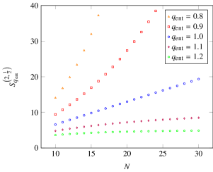
Figure 2: Values of the $S^{\left(2,\alpha\right)}_{q_{\text{ent}}}$ entropy (32) for $\alpha=\frac{1}{2}$ versus $N$ for different values of $q_{\text{ent}}$.

III.2 The $\beta$–numbers and the $\beta$–triangles

Let us consider another deformation of the generalized Leibniz triangles introduced in Section II.

Definition III.4.

Given $n\in\mathds{N}\cup{0}$, and $\beta>0$, $\beta\neq 1$, we shall call $\beta$–numbers the real numbers defined as follows:

$$[n]_{\beta}\coloneqq\begin{cases}0&\text{if $n=0$},\\ n\left(1-\frac{1-\beta}{1-{\beta}^{n}}\right)+1\equiv n\,b_{n}(\beta)&\text{if $n\geq 1$},\end{cases}$$ (33)

where we introduced

$$b_{n}(\beta)\coloneqq 1+\frac{1}{n}-\frac{1-\beta}{1-{\beta}^{n}}.$$ (34)

Note that, so defined, the $\beta$–numbers are related to the $\alpha$–numbers as

$$[n]_{\beta}=\{n-1\}_{\beta}+1.$$ (35)

It follows that $[n]_{1}\coloneqq\lim_{\beta\to 1}[n]_{\beta}=n$, hence the $\beta\to 1$ limit recovers the ordinary numbers. The $\beta$–factorial can now be defined as

$$[0]_{\beta}!\coloneqq 1,\quad[n]_{\beta}!\coloneqq\prod_{k=1}^{n}[k]_{\beta}=n!\prod_{k=1}^{n}b_{k}(\beta),\quad n\geq 1.$$ (36)

The factorial number is recovered as $[n]_{1}!\coloneqq\lim_{\beta\to 1}[n]_{\beta}!=n!$. We can further define the $\beta$–binomial coefficient as

$$\begin{bmatrix}N\\ n\end{bmatrix}_{\beta}\coloneqq\frac{[N]_{\beta}!}{[n]_{\beta}![N-n]_{\beta}!}\\ =\begin{cases}1&\text{if $n=0$ or $n=N$},\\ \binom{N}{n}\prod_{k=1}^{N-n}\frac{b_{k+n}(\beta)}{b_{k}(\beta)}&\text{if $1\leq n\leq N-1$}.\end{cases}$$ (37)

where, as expected, $\lim_{\beta\to 1}\left[\begin{smallmatrix}N\\ n\end{smallmatrix}\right]_{\beta}=\binom{N}{n}$.

We can introduce therefore the Leibniz–like $\beta$–triangle as

$$r^{(1)}_{N,n,\beta}\coloneqq\dfrac{1}{[N+1]_{\beta}}\dfrac{1}{\left[\begin{smallmatrix}N\\ n\end{smallmatrix}\right]_{\beta}},\quad n=0,\dots,N.$$ (38)

The Leibniz triangle (6) is obtained in the $\beta\to 1$ limit, $\lim_{\beta\to 1}r_{N,n,\beta}^{(1)}\equiv r_{N,n}^{(1)}$. As before, in order to get a set of probabilities we have to normalize the triangles, obtaining

$$\hat{r}^{(1)}_{N,n,\beta}\coloneqq\dfrac{r^{(1)}_{N,n,\beta}}{\sum_{k=0}^{N}\binom{N}{k}r^{(1)}_{N,k,\beta}},$$ (39)

whose associated probabilities

$$\hat{p}^{(1)}_{N,n,\beta}\coloneqq\binom{N}{n}\hat{r}^{(1)}_{N,n,\beta}$$ (40)

satisfy by construction the normalization condition $\sum_{n=0}^{N}\hat{p}^{(1)}_{N,n,\beta}=1$.

We will now generalize the Leibniz $\beta$–triangle by properly substracting subtriangles of it. In analogy with the previous deformation, let us now introduce a two–parameter family of triangles

$$r^{(\nu)}_{N,n,\beta}\coloneqq\frac{r^{(1)}_{N+2(\nu-1),n+\nu-1,\beta}}{r^{(1)}_{2(\nu-1),\nu-1,\beta}}\equiv\mu^{(\nu)}_{N,n,\beta}r^{(\nu)}_{N,n},$$ (41)

where $\nu\in\mathds{N}$ and

$$\mu^{(\nu)}_{N,n,\beta}\coloneqq\frac{b_{2\nu-1}(\beta)}{b_{N+2\nu-1}(\beta)}\prod_{k=1}^{\nu-1}\frac{b_{k+\nu-1}(\beta)}{b_{k}(\beta)}\prod_{k=1}^{N-n+\nu-1}\frac{b_{k}(\beta)}{b_{k+n+\nu-1}(\beta)}.$$ (42)

The $\beta\to 1$ limit of the two–parameters family of triangles (41) yields the undeformed family (7), $\lim_{\beta\to 1}r^{(\nu)}_{N,n,\beta}\equiv r^{(\nu)}_{N,n}$. After the needed normalization, we obtain the family $\hat{r}_{N,n,\beta}^{(\nu)}$ and the corresponding probabilities

$$\hat{r}_{N,n,\beta}^{(\nu)} \coloneqq\frac{r_{N,n,\beta}^{(\nu)}}{\sum_{k=0}^{N}\binom{N}{k}r_{N,k,\beta}^{(\nu)}},$$ (43a)

$$\hat{p}_{N,n,\beta}^{(\nu)} \coloneqq\binom{N}{n}\hat{r}_{N,n,\beta}^{(\nu)}.$$ (43b)

It can be proved that the triangle (43a) is asymptotically scale–invariant,

$$\lim_{\begin{subarray}{c}N\to\infty\\ \frac{n}{N}\equiv\eta\ \text{fixed}\end{subarray}}\frac{\hat{r}^{(\nu)}_{N-1,n,\beta}}{\hat{r}^{(\nu)}_{N,n,\beta}+\hat{r}^{(\nu)}_{N,n+1,\beta}}=1.$$ (44)

The $\beta$–numbers appear as a variation of $\alpha$–numbers and, moreover, they have the same asymptotic behavior, $\lim_{n\to\infty}\frac{[n]_{\alpha}}{\{n\}_{\alpha}}=1$. Therefore, it could be expected that the behavior of $\hat{p}^{(\nu)}_{N,n,\alpha}$ is the same of $\hat{p}^{(\nu)}_{N,n,\beta}$ for $N\to\infty$ with respect to the parameters of the deformation. However this is true only when we consider values of the parameters greater than one. Indeed, for $\beta$–triangles, the following theorem holds:

Theorem III.2.

The family of triangles (43) with $\nu\in\mathds{N}$ and $\beta>0$ satisfies the property

$$\frac{N}{2\sqrt{\nu-\chi(\beta)}}\hat{p}_{N,n,\beta}^{(\nu)}\mathbin{\overset{N\gg 1}{\kern 0.0pt\leavevmode\resizebox{22.44292pt}{3.66875pt}{$\sim$}}}P_{q_{\beta}(\nu)}(x),$$ (45)

where we have introduced the function

$$\chi(\beta)\coloneqq 1+\delta_{\beta,1}-\max\left\{1,\frac{1}{\beta}\right\}=\begin{cases}0&\text{for $\beta>1$},\\ 1&\text{for $\beta=1$},\\ 1-\frac{1}{\beta}&\text{for $0<\beta<1$,}\end{cases}$$ (46)

and the properly centered and rescaled variable

$$x\coloneqq 2\sqrt{\nu-\chi(\beta)}\left(\frac{n}{N}-\frac{1}{2}\right).$$ (47)

In Eq. (45), $P_{q_{\beta}(\nu)}(x)$ is a $q$–Gaussian with

$$q_{\beta}(\nu)=1-\frac{1}{\nu-\chi(\beta)}=\begin{cases}1-\frac{1}{\nu}&\text{for $\beta>1$},\\ 1-\frac{1}{\nu-1}&\text{for $\beta=1$},\\ 1-\frac{\beta}{\beta\nu+1-\beta}&\text{for $0<\beta<1$.}\end{cases}$$ (48)

See Appendix B for the proof.

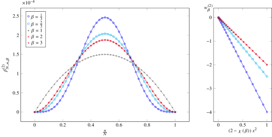
Figure 3: Probability distributions (43b) and $w_{\beta}^{(\nu)}(x)\coloneqq\log_{q_{\beta}(\nu)}\frac{P_{q_{\beta}(\nu)}(x)}{P_{q_{\beta}(\nu)}(0)}$ for $\nu=2$, $N=10^{4}$ and different values of $\beta$; the derived asymptotic behavior is also depicted as continuous line for each value of $\beta$: for the sake of clarity not all data are plotted. The corresponding values of $q_{\beta}(2)$ are given by Eq. (48).

In Fig. 3 we present some numerical results for $\beta$–triangles for different values of $\beta$. We plot also

$$w_{\beta}^{(\nu)}(x)\coloneqq\log_{q_{\beta}(\nu)}\frac{P_{q_{\beta}(\nu)}(x)}{P_{q_{\beta}(\nu)}(0)}$$ (49)

for $\nu=2$ and different values of $\beta$.

Observe that $q_{\alpha}(\nu)=q_{\beta}(\nu)$ when $\alpha>1$ and $\beta>1$; moreover we can write the following relation between the limiting value $q_{\beta}(\nu)$ for the deformed triangles ($\beta\neq 1$) and the limiting value $q_{1}(\nu)$ for the undeformed triangle:

$$\frac{1}{1-q_{\beta}(\nu)}=\frac{1}{1-q_{1}(\nu)}+1-\chi(\beta).$$ (50)

In particular

$$\lim_{\beta\to 1^{\pm}}\frac{1}{1-q_{\beta}(\nu)}=\frac{1}{1-q_{1}(\nu)}+1.$$ (51)

Eq. (50) can be written, for $\beta\neq 1$, as

$$\frac{\min\{\beta,1\}}{1-q_{\beta}(\nu)}=\frac{\min\{\beta,1\}}{1-q_{1}(\nu)}+1.$$ (52)

Finally, following the same arguments adopted for the $\alpha$–triangles, it can be easily verified that also in this case we have $q_{\text{ent}}=1$.

IV A non asymptotically scale–invariant deformation

Inspired by the $Q$–calculus Kac and Cheung (2002), we shall consider an alternative deformation of the Leibniz triangle based on the so called $Q$–numbers, defined as:

$$\llbracket n\rrbracket_{\gamma}\coloneqq\frac{1-\gamma^{n}}{1-\gamma},\quad\gamma\in(0,\infty)\setminus\{1\},$$ (53)

where we have used the notations $\gamma$ and $\llbracket n\rrbracket_{\gamma}$ instead of the usual ones in order to avoid confusion with the entropic index $q$ in nonextensive statistical mechanics and the previously introduced $\alpha$–numbers and $\beta$–numbers. For this reason, in the remainder of the paper we will refer to the $Q$–numbers as the $\gamma$–numbers.

Note that $\gamma$–numbers (53), $\alpha$–numbers (10) and $\beta$–numbers (33) are related as follows:

$$[n]_{\gamma}=\{n-1\}_{\gamma}+1=n\left(1-\frac{1}{\llbracket n\rrbracket_{\gamma}}\right)+1.$$ (54)

In the limit $\gamma\to 1$ the $\gamma$–numbers reduce to the ordinary numbers, $\lim_{\gamma\to 1}[\![n]\!]_{\gamma}=n$. Moreover, a $\gamma$–factorial can be defined as

$$\llbracket 0\rrbracket_{\gamma}!\coloneqq 1,\qquad\llbracket n\rrbracket_{\gamma}!\coloneqq\prod_{k=1}^{n}\llbracket k\rrbracket_{\gamma},\quad\lim_{\gamma\to 1}\llbracket n\rrbracket_{\gamma}!=n!,\quad n\geq 1,$$ (55)

as well as the standard Gauss binomial coefficients

$$\left\llbracket\begin{matrix}N\\ n\end{matrix}\right\rrbracket_{\gamma}\coloneqq\frac{\llbracket N\rrbracket_{\gamma}!}{\llbracket n\rrbracket_{\gamma}!\llbracket N-n\rrbracket_{\gamma}!}\\ =\begin{cases}1&\text{if $n=0$ or $n=N$,}\\ \prod_{k=1}^{N-n}\frac{1-\gamma^{k+n}}{1-\gamma^{k}}&\text{if $0<n<N$},\end{cases}$$ (56)

with $\lim_{\gamma\to 1}\left\llbracket\begin{smallmatrix}N\\ n\end{smallmatrix}\right\rrbracket_{\gamma}=\binom{N}{n}$. The Gauss binomial coefficients can be arranged in a Pascal $\gamma$–triangle:

which reduces to the Pascal triangle for $\gamma\to 1$. We define the Leibniz–like $\gamma$–triangle as:

$$r^{(1)}_{N,n,\gamma}\coloneqq\dfrac{1}{\llbracket N+1\rrbracket_{\gamma}}\dfrac{1}{{\left\llbracket\begin{smallmatrix}N\\ n\end{smallmatrix}\right\rrbracket}_{\gamma}},$$ (57)

with corresponding normalized triangle

$$\hat{r}^{(1)}_{N,n,\gamma}\coloneqq\dfrac{r^{(1)}_{N,n,\gamma}}{\sum_{k=0}^{N}\binom{N}{k}r^{(1)}_{N,k,\gamma}},$$ (58)

and associated probabilities

$$\hat{p}^{(1)}_{N,n,\gamma}\coloneqq\binom{N}{n}\hat{r}^{(1)}_{N,n,\gamma}.$$ (59)

In the limit $\gamma\to 1$, triangles (57) and (58) reduce to the Leibniz triangle.

Proceeding as in the previous Section, we can introduce the family

$$r^{(\nu)}_{N,n,\gamma}\coloneqq\frac{r^{(1)}_{N+2(\nu-1),n+\nu-1,\gamma}}{r^{(1)}_{2(\nu-1),\nu-1,\gamma}},$$ (60)

deformation of the family (7), and the corresponding normalized version and its associated probability

$$\hat{r}^{(\nu)}_{N,n,\gamma} \coloneqq\frac{r^{(\nu)}_{N,n,\gamma}}{\sum_{k=0}^{N}\binom{N}{k}r^{(\nu)}_{N,k,\gamma}},$$ (61a)

$$\hat{p}^{(\nu)}_{N,n,\gamma} \coloneqq\binom{N}{n}\hat{r}^{(\nu)}_{N,n,\gamma}.$$ (61b)

Remarkably, the $\gamma$–triangles (61a) are neither strictly nor asymptotically scale–invariant since

$$\lim_{\begin{subarray}{c}N\to\infty\\ \frac{n}{N}\equiv\eta\text{ fixed}\end{subarray}}\frac{\hat{r}^{(\nu)}_{N-1,n,\gamma}}{\hat{r}^{(\nu)}_{N,n,\gamma}+\hat{r}^{(\nu)}_{N,n+1,\gamma}}=\begin{cases}\frac{1}{2}&\text{for $\gamma<1$,}\\ 0&\text{for $\gamma>1$.}\end{cases}$$ (62)

In addition, probabilities (59) do not approach $q$–Gaussians with $q\neq 1$, as limiting distributions for large values of $N$.

Indeed, let us start from $\gamma\in(0,1)$: for $N\gg 1$, $\nu>1$ and $\frac{n}{N}\equiv\eta$ fixed. Then

$$r^{(\nu)}_{N,n,\gamma}=\frac{1}{r^{(1)}_{2(\nu-1),\nu-1,\gamma}}\frac{1-\gamma}{1-\gamma^{N+2\nu-1}}\cdot\\ \cdot\prod_{k=1}^{N(1-\eta)+\nu-1}\frac{1-\gamma^{k}}{1-\gamma^{k+N\eta+\nu-1}}\\ \sim\frac{(1-\gamma)\prod_{k=1}^{\infty}\left(1-\gamma^{k}\right)}{r^{(1)}_{2(\nu-1),\nu-1,\gamma}}\sim O(1).$$ (63)

The relevant contribution in the probability distribution shape is therefore simply given by the binomial coefficient, and therefore, for $N\gg 1$, we recover the Gaussian distribution (see Fig. 4a) for all values of $\gamma\in(0,1)$:

$$\hat{p}^{(\nu)}_{N,n,\gamma}\mathbin{\overset{N\gg 1}{\kern 0.0pt\leavevmode\resizebox{22.44292pt}{3.66875pt}{$\sim$}}}\sqrt{\frac{2}{\pi N}}e^{-2N\left(\eta-\frac{1}{2}\right)^{2}}.$$ (64)

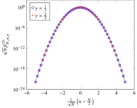
(a) Probability distribution $\hat{p}^{(\nu)}_{N,n,\gamma}$ for $\nu=2$ and different values of $\gamma$ and theoretical prediction for $N=10^{4}$: not all data are represented for sake of clarity.

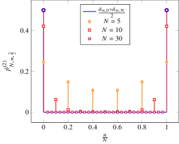
(b) Probability distribution $\hat{p}^{(2)}_{N,n,\frac{3}{2}}$ for different values of $N$.

Figure 4: Numerical results for $\gamma$–triangles.

For $\gamma>1$ we can evaluate the asymptotic distribution as well. We can write

$$\frac{1}{\hat{p}^{(\nu)}_{N,n,\gamma}}=\frac{1}{\binom{N}{n}}\sum_{k=0}^{N}h_{k}(n,N;\gamma)\,,$$ (65)

where

$$\textstyle h_{k}(n,N;\gamma)\coloneqq\begin{cases}\binom{N}{k}\prod^{k-n}_{j=1}\frac{1-\gamma^{n+\nu-1+j}}{1-\gamma^{N-k+\nu-1+j}}&\text{for $k>n$,}\\ \binom{N}{n}&\text{for $k=n$,}\\ \binom{N}{k}\prod^{n-k}_{j=1}\frac{1-\gamma^{N-n+\nu-1+j}}{1-\gamma^{k+\nu-1+j}}&\text{for $k<n$.}\end{cases}$$ (66)

For $N\gg 1$, $\frac{n}{N}\equiv\eta$, and denoting by $\frac{k}{N}\equiv\kappa$, we have that

$$\textstyle h_{N\kappa}(N\eta,N;\gamma)\sim\binom{N}{N\kappa}\gamma^{N^{2}\left(\eta-\kappa\right)\left(1-\eta-\kappa\right)}.$$ (67)

It is easily seen that the quantity $\sum_{N\kappa}\frac{h_{N\kappa}}{\binom{N}{n}}$ can be finite only for $\eta=0$ or $\eta=1$, otherwise at least one of its addends diverges and $\hat{p}_{N,n,\gamma}^{(\nu)}\xrightarrow{N\to\infty}0$, $n=1,\dots,N-1$. Finally we get (see Fig. 4b for a numerical comparison)

$$\hat{p}_{N,n,\gamma}^{(\nu)}\mathbin{\overset{N\gg 1}{\kern 0.0pt\leavevmode\resizebox{22.44292pt}{3.66875pt}{$\sim$}}}\frac{\delta_{n,0}+\delta_{n,N}}{2}.$$ (68)

V Final remarks

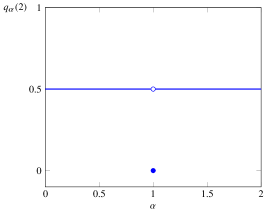
(a) Function $q_{\alpha}(2)$ and its discontinuity for $\alpha=1$, see Eq. (29).

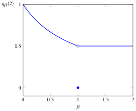
(b) Function $q_{\beta}(2)$ and its discontinuity for $\beta=1$, see Eq. (48).

Figure 5: Functions $q_{\alpha}(\nu)$ and $q_{\beta}(\nu)$ evaluated for $\nu=2$ and different values of $\alpha$ and $\beta$ respectively.

We introduced three deformations — the $\alpha$–, the $\beta$– and the $\gamma$–triangles — of the family of triangles proposed in Rodríguez et al. (2008), in order to analyze the robustness of the $q$–Gaussian family as attractors. Each one of the three proposed deformations depends on a single parameter in such a way that the undeformed family is recovered when the value of that parameter equals $1$. We observed that, in all considered cases, the limiting distribution changes abruptly with respect to the undeformed case when a deformed triangle is considered. Moreover, asymptotically equivalent deformations of natural numbers (the $\alpha$–deformation and the $\beta$–deformation) exhibit different limiting behaviors, thus illustrating the high sensitivity of the limiting distribution with respect to the exact form of the deformation. However, for the considered asymptotically scale–invariant deformations, the limiting distribution of the deformed triangles is still a $q$–Gaussian, with a different value of $q$ generically depending on the parameter of the deformation. Moreover, a discontinuity appears in $q$ as function of the parameters $\alpha,\beta$ of the deformations, in correspondence of the undeformed case $\alpha=\beta=1$ (see Fig. 5). In particular

$$\lim_{\alpha\to 1}\frac{1}{1-q_{\alpha}(\nu)}=\lim_{\beta\to 1}\frac{1}{1-q_{\beta}(\nu)}=\frac{1}{1-q_{1}(\nu)}+1.$$ (69)

Remarkably, this discontinuity appears when we switch from a scale–invariant triangle to an asymptotically scale–invariant triangle. For $\beta$–triangles, and similarly for $\alpha$–triangles, this discontinuity expresses the fact that

$$\lim_{\beta\to 1}\lim_{N\to\infty}N\hat{p}^{(\nu)}_{N,n,\beta}\neq\lim_{N\to\infty}\lim_{\beta\to 1}N\hat{p}^{(\nu)}_{N,n,\beta}.$$ (70)

To exemplify this, let us introduce the following function:

$$\Delta_{N}^{(\nu)}(\beta)\coloneqq\sqrt{N\sum_{n=0}^{N}\left|\hat{p}_{N,n,\beta}^{(\nu)}-p_{N,n}^{(\nu)}\right|^{2}}.$$ (71)

The quantity $\Delta_{N}^{(\nu)}(\beta)$ is defined in such a way that, for $N\to\infty$, it remains finite. Indeed, $N\hat{p}_{N,n,\beta}^{(\nu)}=O(1)$ in the $N\to\infty$ limit, and therefore $\sum_{n=0}^{N}|\hat{p}_{N,n,\beta}^{(\nu)}-p_{N,n}^{(\nu)}|^{2}=O\left(\frac{1}{N}\right)$. In Fig. (6) it can be seen that the convergence of $\Delta_{N}^{(\nu)}(\beta)$ to $\Delta_{\infty}^{(\nu)}(\beta)\coloneqq\lim_{N\to\infty}\Delta_{N}^{(\nu)}(\beta)$ is not uniform and that a discontinuity for $\beta=1$ appears in the $N\to\infty$ limit.

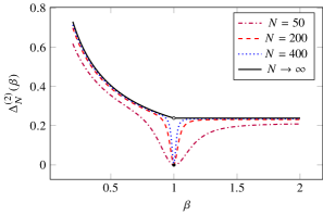
Figure 6: Values of $\Delta_{N}^{(\nu)}(\beta)$ for $\nu=2$ and different values of $N$: the limiting function $\lim_{N\to\infty}\Delta_{N}^{(2)}(\beta)$ is also represented, including its discontinuity for $\beta=1$.

The $\alpha$–triangle is strictly stable under the action of the $\alpha$–deformation for $\alpha\neq 1$, whereas a dependence of the limiting value of $q$ on $\beta$ (for $\beta<1$) appears when the $\beta$–deformation is considered, although the limiting distribution is still a $q$–Gaussian (Marsh et al. (2006) analyzed a probabilistic model in which $q_{\text{ent}}$ has a similar behavior with respect to a certain parameter of the model). The structure of relations (31) and (52) is quite common in the literature: it has been observed, indeed, that for many systems characterized by a set of values of $q$, $\{q_{m}\}_{m\in M}$, $M\coloneqq\{0,1,\dots\}\subseteq\mathds{Z}$, a permutation of the indices $m$ can be found such that $\forall m\in M$ and $\bar{\alpha}\in(0,2]$ Tsallis (2009b)

$$\frac{\bar{\alpha}}{1-q_{m}}=\frac{\bar{\alpha}}{1-q_{0}}+m.$$ (72)

Finally, using the $\gamma$–deformation, that is not an asymptotically scale–invariant deformation, for $\gamma>1$ we obtain a limiting distribution that is not a $q$–Gaussian distribution, and for $\gamma<1$ we always obtain a Gaussian. This fact suggests that the (asymptotic) scale–invariance property plays a central role in the robustness of the set of $q$–Gaussian distributions as limiting distributions. More specifically, the set of $q$–Gaussians appears to be robust under asymptotically scale–invariant deformations. It may be interesting to investigate further the role of asymptotically scale–invariant deformations in the stability of the $q$–Gaussian limiting distributions, to properly identify the conditions under which the basin of $q$–Gaussians is an attractor for these probabilistic models. This line of research could ultimately provide a deeper understanding of why there are so many $q$–Gaussians and $q$–exponentials in Nature.

Appendix A Asymptotic behavior of $\alpha$–triangles

In this Appendix we prove Theorem III.1 on the asymptotic distribution of $\alpha$–triangles. We restate the theorem here for the reader’s convenience.

Theorem.

The family of triangles (20) with $\nu\in(1,+\infty)$ and $\alpha\in\mathds{R}^{+}\setminus\{0\}$ satisfies the property

$$\frac{N}{2\sqrt{\nu-\delta_{\alpha,1}}}\hat{p}_{N,n,\alpha}^{(\nu)}\mathbin{\overset{N\gg 1}{\kern 0.0pt\leavevmode\resizebox{22.44292pt}{3.66875pt}{$\sim$}}}P_{q_{\alpha}(\nu)}(x),$$ (73)

where we have introduced the properly centered and rescaled variable

$$x\coloneqq 2\sqrt{\nu-\delta_{\alpha,1}}\left(\frac{n}{N}-\frac{1}{2}\right).$$ (74)

In Eq. (73), $P_{q_{\alpha}(\nu)}(x)$ is a $q$–Gaussian with

$$q_{\alpha}(\nu)\coloneqq 1-\frac{1}{\nu-\delta_{\alpha,1}}=\begin{cases}1-\frac{1}{\nu}&\text{for $\alpha\neq 1$},\\ 1-\frac{1}{\nu-1}&\text{for $\alpha=1$.}\end{cases}$$ (75)

Proof.

The strategy of the first part of the proof consists in a generalization of the argument in Rodríguez et al. (2008). We want to evaluate the asymptotic behavior, for $N\gg 1$, of

$$\binom{N}{n}r^{(\nu)}_{N,n,\alpha}$$ (76)

with $\eta\coloneqq\frac{n}{N}$ fixed. Let us firstly observe that

$$r^{(\nu)}_{N,0}=\frac{\Gamma(2\nu)\Gamma(N+\nu)}{\Gamma(\nu)\Gamma(N+2\nu)}=\frac{\Gamma(2\nu)}{\Gamma^{2}(\nu)}\sum_{k=0}^{\infty}\frac{(1-\nu)_{k}}{k!(N+\nu+k)},$$ (77)

where we used the formula for the beta function

$$\mathrm{B}(a,b)\coloneqq\frac{\Gamma(a)\Gamma(b)}{\Gamma(a+b)}=\int_{0}^{1}t^{a-1}(1-t)^{b-1}dt=\sum_{k=0}^{\infty}\frac{(1-b)_{k}}{k!(a+k)},$$ (78)

and $(a)_{k}\coloneqq a(a+1)\dots(a+k-1)$ is the rising factorial. The previous formula allows us to write down a general expression for the element $r^{(\nu)}_{N,n}$ as follows:

$$r^{(\nu)}_{N,n}=\sum_{i=0}^{n}(-1)^{n-i}\binom{n}{i}r^{(\nu)}_{N-i,0}\\ =\frac{\Gamma(2\nu)}{\Gamma^{2}(\nu)}\sum_{i=0}^{n}\sum_{k=0}^{\infty}\frac{(-1)^{n-i}(1-\nu)_{k}}{k!}\binom{n}{i}\frac{1}{N+\nu-i+k}.$$ (79)

To evaluate the large $N$ behavior, we use the saddle point approximation,

$$\sum_{i=0}^{n}(-1)^{n-i}\binom{n}{i}\frac{1}{N+\nu-i+k}\\ =\int_{0}^{\infty}\left(e^{\xi}-1\right)^{n}e^{-(N+\nu+k)\xi}d\xi\\ \sim\sqrt{\frac{2\pi}{N}}\left(1-\eta\right)^{\nu+k+N(1-\eta)-\frac{1}{2}}\eta^{N\eta+\frac{1}{2}},$$ (80)

where $\eta\coloneqq\frac{n}{N}$. Inserting the previous term in the complete expression we have

$$r_{N,n}^{(\nu)}\sim\frac{\Gamma(2\nu)}{\Gamma^{2}(\nu)}\sqrt{\frac{2\pi}{N}}\left(1-\eta\right)^{\nu+N(1-\eta)-\frac{1}{2}}\eta^{\nu+N\eta-\frac{1}{2}}$$ (81)

Moreover, using the Stirling formula,

$$N\binom{N}{n}\mathbin{\overset{N\gg 1}{\kern 0.0pt\leavevmode\resizebox{22.44292pt}{3.66875pt}{$\sim$}}}\sqrt{\frac{N}{2\pi}}(1-\eta)^{-N(1-\eta)-\frac{1}{2}}\eta^{-N\eta-\frac{1}{2}}\\ \Rightarrow N\binom{N}{n}r^{(\nu)}_{N,n}\mathbin{\overset{N\gg 1}{\kern 0.0pt\leavevmode\resizebox{22.44292pt}{3.66875pt}{$\sim$}}}\frac{\Gamma(2\nu)}{\Gamma^{2}(\nu)}\left[\left(1-\eta\right)\eta\right]^{\nu-1}.$$ (82)

To complete the proof, we only need to evaluate the asymptotic behavior of $\mu^{(\nu)}_{N,n,\alpha}$ for large $N$ at fixed $\eta$. Obviously, $\lim_{\alpha\to 1}\mu^{(\nu)}_{N,n,\alpha}=1$. For $\alpha\neq 1$ we have that, by direct computation on the expression (22)

$$\mu^{(\nu)}_{N,n,\alpha}\mathbin{\overset{N\gg 1}{\kern 0.0pt\leavevmode\resizebox{22.44292pt}{3.66875pt}{$\sim$}}}N\eta(1-\eta)$$ (83)

up to a multiplicative constant depending on $\alpha$ and $\nu$. The thesis follows straightforwardly after a proper change of variable, $\eta\mapsto\frac{x}{2\sqrt{\nu-\delta_{\alpha,1}}}+\frac{1}{2}$, and normalization. Observe also that the thesis holds for all real values $\nu>1$. ∎

Appendix B Asymptotic behavior of $\beta$–triangles

In this Appendix we prove Theorem III.2 on the asymptotic distribution of $\beta$–triangles. We restate the theorem here for the reader’s convenience.

Theorem.

The family of triangles (43b) with $\nu\in\mathds{N}$ and $\beta>0$ satisfies the property

$$\frac{N}{2\sqrt{\nu-\chi(\beta)}}\hat{p}_{N,n,\beta}^{(\nu)}\mathbin{\overset{N\gg 1}{\kern 0.0pt\leavevmode\resizebox{22.44292pt}{3.66875pt}{$\sim$}}}P_{q_{\beta}(\nu)}(x),$$ (84)

where we have introduced the function

$$\chi(\beta)\coloneqq 1+\delta_{\beta,1}-\max\left\{1,\frac{1}{\beta}\right\}=\begin{cases}0&\text{for $\beta>1$},\\ 1&\text{for $\beta=1$},\\ 1-\frac{1}{\beta}&\text{for $0<\beta<1$,}\end{cases}$$ (85)

and the properly centered and rescaled variable

$$x\coloneqq 2\sqrt{\nu-\chi(\beta)}\left(\frac{n}{N}-\frac{1}{2}\right).$$ (86)

In Eq. (84), $P_{q_{\beta}(\nu)}(x)$ is a $q$–Gaussian with

$$q_{\beta}(\nu)=1-\frac{1}{\nu-\chi(\beta)}=\begin{cases}1-\frac{1}{\nu}&\text{for $\beta>1$},\\ 1-\frac{1}{\nu-1}&\text{for $\beta=1$},\\ 1-\frac{\beta}{\beta\nu+1-\beta}&\text{for $0<\beta<1$.}\end{cases}$$ (87)

Proof.

The proof of the Theorem strictly follows the proof of Theorem III.1 in A, the only difference being the evaluation of the asymptotic behavior of the $\mu^{(\nu)}_{N,n,\beta}$ coefficient for large $N$ at fixed $\frac{n}{N}$.

For $\beta=1$, we have simply $\mu^{(\nu)}_{N,n,1}=1$ so there is nothing to do.

For $\beta\neq 1$ and $\nu=2,3,\dots$, denoting $N-n\eqqcolon N\eta$, we can write

$$\mu^{(\nu)}_{N,n,\beta}=\prod_{k=0}^{\nu-1}b_{k+\nu}(\beta)\frac{\prod_{k=0}^{N\eta-1}b_{k+\nu}(\beta)}{\prod_{k=0}^{N\eta-1+\nu}b_{k+\nu+N(1-\eta)}(\beta)}.$$ (88)

Observe that the first product

$$B_{0}\coloneqq\prod_{k=0}^{\nu-1}b_{k+\nu}(\beta)$$ (89)

is only a global factor not depending on $N,n$. We need to perform our asymptotic analysis only on the fraction

$$\frac{\prod_{k=0}^{N\eta-1}b_{k+\nu}(\beta)}{\prod_{k=0}^{N\eta-1+\nu}b_{k+\nu+N(1-\eta)}(\beta)}.$$ (90)

We distinguish the two cases, $0<\beta<1$ and $\beta>1$.

For $0<\beta<1$

$$\mu^{(\nu)}_{N,n,\beta}\mathbin{\overset{N\gg 1}{\kern 0.0pt\leavevmode\resizebox{22.44292pt}{3.66875pt}{$\sim$}}}B_{-}N^{\frac{1}{\beta}}\left[\eta(1-\eta)\right]^{\frac{1}{\beta}},$$ (91)

where $B_{-}$ is a certain constant. Indeed we have that the asymptotic behavior of the denominator of the fraction (90) can be evaluated as

$$\frac{1}{\prod_{k=0}^{N\eta-1+\nu}b_{k+\nu+N(1-\eta)}(\beta)}\\ \sim\frac{1}{\beta^{N\eta+\nu}}\prod_{k=0}^{N\eta-1+\nu}\left(1-\frac{1}{\beta}\frac{1}{k+\nu+N(1-\eta)}\right)\\ \textstyle\\ =\frac{\Gamma\left(N+2\nu-\frac{1}{\beta}\right)}{\beta^{N\eta+\nu}\Gamma(N+2\nu)}\frac{\Gamma\left(N(1-\eta)+\nu\right)}{\Gamma\left(N(1-\eta)+\nu-\frac{1}{\beta}\right)}\sim\frac{(1-\eta)^{\frac{1}{\beta}}}{\beta^{N\eta+\nu}}.$$ (92)

Moreover, we have also

$$\prod_{k=0}^{N\eta-1}b_{k+\nu}(\beta)=\\ =\beta^{N\eta}\prod_{k=0}^{N\eta-1}\frac{b_{k+\nu}(\beta)}{\beta}=\beta^{N\eta}\prod_{k=1}^{\infty}\frac{b_{k+\nu}(\beta)}{\beta b^{\prime}_{k+\nu}(\beta)}.$$ (93)

In the previous expression we introduced

$$b^{\prime}_{k+\nu}(\beta)\coloneqq\begin{cases}1&\text{for $1\leq k\leq N\eta-1$,}\\ \frac{b_{k+\nu}(\beta)}{\beta}&\text{for $k\geq N\eta$.}\end{cases}$$ (94)

In the large $N$ limit we have that

$$\prod_{k=0}^{N\eta-1}b_{k+\nu}(\beta)=\beta^{N\eta}\prod_{k=1}^{\infty}\frac{b_{k+\nu}(\beta)}{\beta b^{\prime}_{k+\nu}(\beta)}\\ \mathbin{\overset{N\gg 1}{\kern 0.0pt\leavevmode\resizebox{22.44292pt}{3.66875pt}{$\sim$}}}\beta^{N\eta}\prod_{k=1}^{\infty}\frac{b_{k+\nu}(\beta)}{\beta b^{\prime\prime}_{k+\nu}(\beta)}=\beta^{N\eta}B_{1}(\beta)\prod_{k=1}^{N\eta-1}\left(1+\frac{1}{\beta(k+\nu)}\right)\\ =B_{1}(\beta)\beta^{N\eta}\frac{\Gamma(\nu)}{\Gamma\left(\nu+\frac{1}{\beta}\right)}\frac{\Gamma\left(N\eta+\nu+\frac{1}{\beta}\right)}{\Gamma\left(N\eta+\nu\right)}\\ \sim B_{1}(\beta)B_{2}(\beta)\beta^{N\eta}N^{\frac{1}{\beta}}\eta^{\frac{1}{\beta}},$$ (95)

where we have introduced

$$b^{\prime\prime}_{k+\nu}(\beta)\coloneqq\begin{cases}1&\text{for $1\leq k\leq N\eta-1$,}\\ 1+\frac{1}{\beta(k+\nu)}&\text{for $k\geq N\eta$,}\end{cases}$$ (96)

and the constants

$$B_{1}(\beta) \coloneqq\prod_{k=0}^{\infty}\frac{1+\frac{1}{k+\nu}-\frac{1-\beta}{1-\beta^{k+\nu}}}{\min\{\beta,1\}+\frac{1}{k+\nu}},$$ (97a)

$$B_{2}(\beta) \coloneqq\frac{\Gamma(\nu)}{\Gamma\left(\nu+\frac{1}{\beta}\right)e^{\frac{1}{\beta}}}.$$ (97b)

Eq. (91) follows directly identifying $B_{-}\equiv B_{1}(\beta)B_{2}(\beta)$.

For $\beta>1$ we have instead that

$$\mu^{(\nu)}_{N,n,\beta}\mathbin{\overset{N\gg 1}{\kern 0.0pt\leavevmode\resizebox{22.44292pt}{3.66875pt}{$\sim$}}}B_{+}N\eta(1-\eta),$$ (98)

where $B_{+}$ is a certain constant depending on $\beta$. Indeed, in Eq. (88) we can write

$$\frac{\prod_{k=0}^{N\eta-1}b_{k+\nu}(\beta)}{\prod_{k=0}^{N\eta-1+\nu}b_{k+\nu+N(1-\eta)}(\beta)}\\ \sim\prod_{k=0}^{N\eta-1}b_{k+\nu}(\beta)\prod_{k=0}^{N\eta-1+\nu}\left(1-\frac{1}{k+\nu+N(1-\eta)}\right)\\ =\frac{N(1-\eta)+\nu-1}{N+2\nu-1}\prod_{k=0}^{N\eta-1}b_{k+\nu}(\beta)\sim(1-\eta)\prod_{k=0}^{N\eta-1}b_{k+\nu}(\beta).$$ (99)

The remaining product can be written similarly as

$$\prod_{k=0}^{N\eta-1}b_{k+\nu}(\beta)\sim B_{1}(\beta)\prod_{k=0}^{N\eta-1}\left(1+\frac{1}{k+\nu}\right)\sim B_{1}(\beta)B_{2}(1)N\eta,$$ (100)

where we used the definitions (97). Eq. (98) follows directly imposing $B_{+}\equiv B_{1}(\beta)B_{2}(1)$.

Summarizing, for $\beta>0$, $\beta\neq 1$, up to a global multiplicative constant,

$$\mu^{(\nu)}_{N,n,\beta}\mathbin{\overset{N\gg 1}{\kern 0.0pt\leavevmode\resizebox{22.44292pt}{3.66875pt}{$\sim$}}}\left[N\eta(1-\eta)\right]^{\max\left\{1,\frac{1}{\beta}\right\}-\delta_{\beta,1}}.$$ (101)

Defining the function $\chi(\beta)$ as in (85), we have

$$N^{\chi(\beta)}\binom{N}{n}r^{(\nu)}_{N,n,\beta}\mathbin{\overset{N\gg 1}{\kern 0.0pt\leavevmode\resizebox{22.44292pt}{3.66875pt}{$\sim$}}}\left[\eta(1-\eta)\right]^{\nu-\chi(\beta)}.$$ (102)

Introducing now the variable

$$x\coloneqq 2\sqrt{\nu-\chi(\beta)}\left(\eta-\frac{1}{2}\right)$$ (103)

and properly normalizing we obtain the thesis. ∎

References

- Andrade Jr et al. (2010) Andrade Jr, J., Da Silva, G., Moreira, A., Nobre, F., Curado, E., 2010. Thermostatistics of overdamped motion of interacting particles. Physical Review Letters 105 (26), 260601.
- Anteneodo and Tsallis (1998) Anteneodo, C., Tsallis, C., 1998. Breakdown of exponential sensitivity to initial conditions: Role of the range of interactions. Physical Review Letters 80 (24), 5313.
- Boghosian (1996) Boghosian, B. M., 1996. Thermodynamic description of the relaxation of two-dimensional turbulence using Tsallis statistics. Physical Review E 53 (5), 4754.
- Borland (2002) Borland, L., 2002. Option pricing formulas based on a non–Gaussian stock price model. Physical Review Letters 89 (9), 098701.
- Cirto et al. (2014) Cirto, L. J., Assis, V. R., Tsallis, C., 2014. Influence of the interaction range on the thermostatistics of a classical many–body system. Physica A: Statistical Mechanics and its Applications 393, 286–296.
- Douglas et al. (2006) Douglas, P., Bergamini, S., Renzoni, F., 2006. Tunable tsallis distributions in dissipative optical lattices. Physical review letters 96 (11), 110601.
- Feller (1971) Feller, W., 1971. An Introduction to Probability Theory and Its Applications. Vol. 2. John Wiley and Sons, New York.
- Hahn et al. (2010) Hahn, M. G., Jiang, X., Umarov, S., 2010. On –Gaussians and exchangeability. Journal of Physics A: Mathematical and Theoretical 43 (16), 165208.
- Hanel and Thurner (2011a) Hanel, R., Thurner, S., 2011a. A comprehensive classification of complex statistical systems and an axiomatic derivation of their entropy and distribution functions. Europhysics Letters 93 (2), 20006.
- Hanel and Thurner (2011b) Hanel, R., Thurner, S., 2011b. When do generalized entropies apply? How phase space volume determines entropy. Europhysics Letters 96 (5), 50003.
- Hanel et al. (2009) Hanel, R., Thurner, S., Tsallis, C., 2009. Limit distributions of scale–invariant probabilistic models of correlated random variables with the –Gaussian as an explicit example. The European Physical Journal B – Condensed Matter and Complex Systems 72 (2), 263–268.
- Hilhorst and Schehr (2007) Hilhorst, H., Schehr, G., 2007. A note on –Gaussians and non–Gaussians in statistical mechanics. Journal of Statistical Mechanics: Theory and Experiment 2007 (06), P06003.
- Kac and Cheung (2002) Kac, V., Cheung, P., 2002. Quantum Calculus. Springer Science & Business Media.
- Leo et al. (2012) Leo, M., Leo, R., Tempesta, P., Tsallis, C., 2012. Non-maxwellian behavior and quasistationary regimes near the modal solutions of the fermi-pasta-ulam system. Physical Review E 85 (3), 031149.
- Lutz (2003) Lutz, E., 2003. Anomalous diffusion and tsallis statistics in an optical lattice. Physical Review A 67 (5), 051402.
- Lutz and Renzoni (2013) Lutz, E., Renzoni, F., 2013. Beyond Boltzmann-Gibbs statistical mechanics in optical lattices. Nature Physics 9 (10), 615–619.
- Marsh et al. (2006) Marsh, J. A., Fuentes, M. A., Moyano, L. G., Tsallis, C., 2006. Influence of global correlations on central limit theorems and entropic extensivity. Physica A: Statistical Mechanics and its Applications 372 (2), 183–202.
- Pluchino et al. (2007) Pluchino, A., Rapisarda, A., Tsallis, C., 2007. Nonergodicity and central–limit behavior for long–range Hamiltonians. Europhysics Letters 80 (2), 26002.
- Polya (1962) Polya, G., 1962. Mathematical Discovery. Vol. 1. John Wiley and Sons, New York.
- Rodríguez et al. (2008) Rodríguez, A., Schwämmle, V., Tsallis, C., 2008. Strictly and asymptotically scale invariant probabilistic models of correlated binary random variables having –Gaussians as limiting distributions. Journal of Statistical Mechanics: Theory and Experiment 2008 (09), P09006.
- Rodríguez and Tsallis (2012) Rodríguez, A., Tsallis, C., 2012. A dimension scale–invariant probabilistic model based on Leibniz–like pyramids. Journal of Mathematical Physics 53 (2), 023302.
- Rodríguez and Tsallis (2014) Rodríguez, A., Tsallis, C., 2014. Connection between Dirichlet distributions and a scale–invariant probabilistic model based on Leibniz–like pyramids. Journal of Statistical Mechanics: Theory and Experiment 2014 (12), P12027.
- Tempesta (2011) Tempesta, P., 2011. Group entropies, correlation laws, and zeta functions. Physical Review E 84 (2), 021121.
- Tempesta (2014) Tempesta, P., 2014. Beyond the Shannon–Khinchin formulation: The composability axiom and the universal–group entropy. arXiv preprint arXiv:1407.3807.
- Tirnakli et al. (2007) Tirnakli, U., Beck, C., Tsallis, C., 2007. Central limit behavior of deterministic dynamical systems. Physical Review E 75 (4), 040106.
- Tirnakli and Borges (2015) Tirnakli, U., Borges, E. P., 2015. The standard map: From Boltzmann–Gibbs statistics to Tsallis statistics. arXiv:1501.02459.
- Tsallis (1988) Tsallis, C., 1988. Possible generalization of Boltzmann–Gibbs statistics. Journal of Statistical Physics 52 (1-2), 479–487.
- Tsallis (2009a) Tsallis, C., 2009a. Introduction to Nonextensive Statistical Mechanics. Springer.
- Tsallis (2009b) Tsallis, C., 2009b. Nonadditive entropy and nonextensive statistical mechanics – An overview after 20 years. Brazilian Journal of Physics 39 (2A), 337–356.
- Tsallis et al. (2003) Tsallis, C., Anteneodo, C., Borland, L., Osorio, R., 2003. Nonextensive statistical mechanics and economics. Physica A: Statistical Mechanics and its Applications 324 (1), 89–100.
- Tsallis and Bukman (1996) Tsallis, C., Bukman, D. J., 1996. Anomalous diffusion in the presence of external forces: Exact time-dependent solutions and their thermostatistical basis. Physical Review E 54 (3), R2197.
- Tsallis et al. (2005) Tsallis, C., Gell-Mann, M., Sato, Y., 2005. Asymptotically scale–invariant occupancy of phase space makes the entropy extensive. Proceedings of the National Academy of Sciences of the United States of America 102 (43), 15377–15382.
- Umarov et al. (2010) Umarov, S., Tsallis, C., Gell-Mann, M., Steinberg, S., 2010. Generalization of symmetric –stable Lévy distributions for . Journal of Mathematical Physics 51 (3), 033502.
- Umarov et al. (2008) Umarov, S., Tsallis, C., Steinberg, S., 2008. On a –central limit theorem consistent with nonextensive statistical mechanics. Milan Journal of Mathematics 76 (1), 307–328.
- Upadhyaya et al. (2001) Upadhyaya, A., Rieu, J.-P., Glazier, J. A., Sawada, Y., 2001. Anomalous diffusion and non-Gaussian velocity distribution of Hydra cells in cellular aggregates. Physica A: Statistical Mechanics and its Applications 293 (3), 549–558.
- Vignat and Plastino (2007) Vignat, C., Plastino, A., 2007. Central limit theorem and deformed exponentials. Journal of Physics A: Mathematical and Theoretical 40 (45), F969.
- Wong and Wilk (2013) Wong, C.-Y., Wilk, G., 2013. Tsallis fits to spectra and multiple hard scattering in collisions at the LHC. Physical Review D 87 (11), 114007.