A kinetic theory for age-structured stochastic birth-death processes

Abstract

Classical age-structured mass-action models such as the McKendrick-von Foerster equation have been extensively studied but they are structurally unable to describe stochastic fluctuations or population-size-dependent birth and death rates. Stochastic theories that treat semi-Markov age-dependent processes using e.g., the Bellman-Harris equation, do not resolve a population’s age-structure and are unable to quantify population-size dependencies. Conversely, current theories that include size-dependent population dynamics (e.g., mathematical models that include carrying capacity such as the Logistic equation) cannot be easily extended to take into account age-dependent birth and death rates. In this paper, we present a systematic derivation of a new fully stochastic kinetic theory for interacting age-structured populations. By defining multiparticle probability density functions, we derive a hierarchy of kinetic equations for the stochastic evolution of an ageing population undergoing birth and death. We show that the fully stochastic age-dependent birth-death process precludes factorization of the corresponding probability densities, which then must be solved by using a BBGKY-like hierarchy. However, explicit solutions are derived in two simple limits and compared with their corresponding mean-field results. Our results generalize both deterministic models and existing master equation approaches by providing an intuitive and efficient way to simultaneously model age- and population-dependent stochastic dynamics applicable to the study of demography, stem cell dynamics, and disease evolution.

I Introduction

Age is an important controlling feature in populations of living organisms. Processes such as birth, death, and mutation are typically highly dependent upon an organism’s chronological age. Age-dependent population dynamics, where birth and death probabilities depend on an organism’s age, arise across diverse research areas such as demography Keyfitz and Caswell (2005), biofilm formation Ayati (2007), and stem cell proliferation and differentiation Stukalin et al. (2013); Roshan et al. (2014). In this latter application, not only does a the cell cycle give rise to age-dependent processes Qu et al. (2003); Weber et al. (2014), but the often small number of cells requires a stochastic interpretation of the population. Despite the importance of age structure (such as that arising in the study of cell cycles Qu et al. (2003); Weber et al. (2014); Oh et al. (2014)), there exists no theoretical method to fully quantify the stochastic dynamics of aging and population-dependent processes.

Past work on age-structured populations has focussed on deterministic models through the analysis of the so-called McKendrick-von Foerster equation, first studied by McKendrick McKendrick (1926); Keyfitz and Keyfitz (1997) and subsequently von Foerster von Foerster (1959), Gurtin and MacCamy Gurtin and MacCamy (1974, 1979), and others Iannelli (1995); Webb (2008). In these classic treatments, $\rho(a,t)\mbox{d}a$ is used to define, at time $t$, the density of noninteracting agents with age between $a$ and $a+\mbox{d}a$. The total number of particles in the system at time $t$ is thus $n(t)=\int_{0}^{\infty}\rho(a,t)\mbox{d}a$. If $\mu(a;n(t))$ is the death rate for individuals of age $a$, the McKendrick-von Foerster equations are Gurtin and MacCamy (1974, 1979)

$${\partial\rho(a,t)\over\partial t}+{\partial\rho(a,t)\over\partial a}=-\mu(a;n(t))\rho(a,t),$$ (1)

with $\rho(a,t=0)=g(a)$ and

$$\rho(a=0,t)=\int_{0}^{\infty}\beta(a;n(t))\rho(a,t)\mbox{d}a$$ (2)

for initial and boundary conditions, respectively. The boundary condition (Eq. 2) reflects the fact that birth gives rise to age-zero individuals. Note that the birth and death rates $\beta$ and $\mu$ are usually simply assumed to be functions of the total population $n(t)$.

The population dependence of $\beta(a;n(t))$ and $\mu(a;n(t))$ in Eqs. 1 and 2 are assumed without explicit derivation and it is not clear whether such simple expressions are self-consistent. Moreover, the McKendrick-von Foerster equation is expected to be accurate exact only when the dynamics of each individual are not correlated with those of any other. Therefore, a formal derivation will allow a deeper understanding of how population dependence and correlations arise in a fully stochastic age-structured framework.

Two approaches that have been used for describing stochastic populations include Master equations Kampen (2011); Chou and D’Orsogna (2014) and evolution equations for age-dependent branching process such as the Bellman-Harris process Bellman and Harris (1948); Reid (1953); Jagers (1968); Shonkwiler (1980); Chou and Wang (2015). Master-equation approaches can be used to describe population-dependent birth or death rates Kendall (1948); Gurtin and MacCamy (1974, 1979); Allen (2003) but implicitly assume exponentially distributed waiting times between events Chou and D’Orsogna (2014). On the other hand, age-dependent models such as the Bellman-Harris branching process Bellman and Harris (1948) allow for arbitrary distributions of times between birth/death events but they cannot resolve age-structure of the entirte population nor describe population-dependent dynamics that arise from e.g., regulation or environmental carrying capacities.

A number of approaches attempt to incorporate ideas of stochasticity and noise into age-dependent population models, Stukalin et al. (2013); Reid (1953); Chowdhury (1998); Li et al. (2009); Getz (1984); Cohen et al. (1983); Leslie (1945, 1948). For example, stochasticity can be implemented by assuming a random rate of advancing to the next age window (by e.g., stochastic harvesting Getz (1984); Cohen et al. (1983) or a fluctuating environment Lande and Orzack (1988); Engen et al. (2005)). However, such models do not account for the intrinsic stochasticity of the underlying birth-death process that acts differently on individuals at each different age. One alternative approach might be to extend the mean-field, age-structured McKendrick-von Foerster theory into the stochastic domain by considering the evolution of $P(n(a);t)$, the probability density that there are $n$ individuals within age window $[a,a+\mbox{d}a]$ at time $t$ Stukalin et al. (2013); Pollard (1966). This approach is meaningful only if a large number of individuals exist in each age window, in which case a large system size van Kampen expansion within each age window can be applied Kampen (2011). However, such an assumption is inconsistent with the desired small-number stochastic description of the system.

A mathematical theory that addresses the age-dependent problem of constrained stochastic populations would provide an important tool for quantitatively investigating problems in demography, bacterial growth, population biology, and stem cell differentiation and proliferation. In this paper, we develop a new kinetic equation that intuitively integrates population stochasticity, age-dependent effects (such as cell cycle), and population regulation into a unified theory. Our equations form a hierarchy analogous to that derived for the BBGKY (Bogoliubov-Born-Green-Kirkwood-Yvon) hierarchy in kinetic theory McQuarrie (2000); Zanette (1990), allowing for a fully stochastic treatment of age-dependent process undergoing population-dependent birth and death.

II Kinetic equations for aging populations

To develop a fully stochastic theory for age-structured populations that can naturally describe both age- and population size-dependent birth and death rates, we invoke multiple-particle distribution functions such as those used in kinetic theories of gases Zanette (1990). Our analysis builds on the Boltzmann kinetic theory of D. Zanette and yields a BBGKY-like hierarchy of equations. Here, the positions of ballistic particles will represent the ages of individuals.

Changes in the total population require that we consider a family of multiparticle distribution functions, each with different dimensionality corresponding to the number of individuals. In this picture, birth and death are represented by transitions between the different distribution functions residing on different fixed particle-number “manifolds.” Processes that generate newborns (particles of age zero) manifest themselves mathematically through boundary conditions on higher dimensional distribution functions.

To begin, we define

$$f_{n}(x_{1},x_{2},x_{3},\ldots,x_{n};t)\mbox{d}x_{1}\mbox{d}x_{2}\ldots\mbox{d}x_{n}$$ (3)

as the probability that at time $t$, one observes $n$ distinguishable (by virtue of their order of birth) individuals, such that the youngest one has age within $(x_{1},x_{1}+\mbox{d}x_{1})$, the second youngest has age within $(x_{2},x_{2}+\mbox{d}x_{2})$, and so on. If the individuals are identical (except for their ages) and one does not distinguish which are in each age window, one can define $\rho_{n}(x_{1},x_{2},x_{3},\ldots,x_{n};t)\mbox{d}x_{1}\mbox{d}x_{2}\ldots\mbox{d}x_{n}$ as the probability that after randomly selecting individuals, the first one chosen has age in $(x_{1},x_{1}+\mbox{d}x_{1})$, the second has age in $(x_{2},x_{2}+\mbox{d}x_{2})$, and so on. For example, if there are three individuals with ordered ages $x_{1}<x_{2}<x_{3}$, the probability of making any specific random selection, such as choosing the individual with age $x_{2}$ first, the one with age $x_{1}$ second, and the one with age $x_{3}$ third, is $\frac{1}{3!}$. More generally, when the ages ${\bf x}_{1,n}\equiv{\bf x}_{n}=(x_{1},x_{2},\ldots,x_{n})$ are unordered, the associated probability density is

$$\rho_{n}({\bf x}_{n};t)=\frac{1}{n!}f_{n}({\cal T}(\{x_{i}\});t),$$ (4)

in which ${\cal T}$ is the time-ordering permutation operator such that, for example, ${\cal T}(x_{2},x_{1},x_{3})=(x_{1},x_{2},x_{3})$. Note that in this formulation, $\rho_{n}({\bf x}_{n};t)$ is invariant under interchange of the elements of ${\bf x}_{n}$.

To derive kinetic equations for $\rho_{n}({\bf x}_{n};t)$, we first define an ordered cumulative probability distribution

$$Q_{n}({\bf a}_{n};t)=\int_{0}^{a_{1}}\mbox{d}x_{1}\int_{x_{1}}^{a_{2}}\mbox{d}x_{2}\cdots\int_{x_{n-1}}^{a_{n}}\!\!\!\mbox{d}x_{n}f_{n}({\bf x}_{n};t),$$ (5)

where ${\bf a}_{n}=a_{1,n}=(a_{1},\ldots,a_{n})$. $Q_{n}({\bf a}_{n};t)$ describes the probability that there are $n$ existing individuals at time $t$ and that the youngest individual has age $x_{1}$ less than or equal to $a_{1}$, the second youngest individual has age $x_{1}\leq x_{2}<a_{2}$, and so on. The oldest individual has age $x_{n-1}\leq x_{n}\leq a_{n}$.

We now compute the change in $Q_{n}({\bf a}_{n};t)$ over a small time increment $\varepsilon$: $Q_{n}({\bf a}_{n}+\varepsilon;t+\varepsilon)=Q_{n}({\bf a}_{n};t)+\int_{t}^{t+\varepsilon}J({\bf a}_{n};t^{\prime})\mbox{d}t^{\prime}$, where $J({\bf a}_{n};t^{\prime})=J^{+}({\bf a}_{n};t^{\prime})-J^{-}({\bf a}_{n};t^{\prime})$ is the net probability flux at time $t^{\prime}$. The probability flux which increases the cumulative probability is denoted $J^{+}$ while that which decrease the cumulative probability is labelled $J^{-}$. Each of the $J^{\pm}$ include contributions from different processes that remove or add individuals. A schematic of our birth-death process, starting from a single parent, is depicted in Fig. 1A.

In the $\varepsilon\to 0$ limit, we find the conservation equation

$${\partial Q_{n}({\bf a}_{n};t)\over\partial t}+\sum_{i=1}^{n}{\partial Q_{n}({\bf a}_{n};t)\over\partial a_{i}}=J^{+}({\bf a}_{n};t)-J^{-}({\bf a}_{n};t).$$ (6)

Eq. 6 is a “weak form” integral equation for the probability density which allows us to systematically derive an evolution equation and the associated boundary conditions for $f_{n}({\bf x}_{n};t)$. The probability fluxes can be decomposed into components representing age-dependent birth and death

$$J^{\pm}({\bf a}_{n};t)=J^{\pm}_{\beta}({\bf a}_{n};t)+J^{\pm}_{\mu}({\bf a}_{n};t),$$ (7)

where the birth and death that reduce probability can be expressed as

$$\displaystyle J^{-}_{\beta}({\bf a}_{n};t)=\displaystyle\int_{0}^{a_{1}}\!\!\mbox{d}x_{1}\int_{x_{1}}^{a_{2}}\!\!\mbox{d}x_{2}\cdots\!\int_{x_{n-1}}^{a_{n}}\!\!\!\!\!\mbox{d}x_{n}f_{n}({\bf x}_{n};t)\sum_{i=1}^{n}\beta_{n}(x_{i}),$$ (8)

$$\displaystyle J^{-}_{\mu}({\bf a}_{n};t)=\displaystyle\int_{0}^{a_{1}}\!\!\mbox{d}x_{1}\int_{x_{1}}^{a_{2}}\!\!\mbox{d}x_{2}\cdots\!\int_{x_{n-1}}^{a_{n}}\!\!\!\!\!\mbox{d}x_{n}f_{n}({\bf x}_{n};t)\sum_{i=1}^{n}\mu_{n}(x_{i}).$$ (9)

Similarly, the probability fluxes that increase probability are

$$\displaystyle J^{+}_{\beta}({\bf a}_{n};t)= \int_{0}^{a_{2}}\!\!\mbox{d}x_{1}\cdots\!\int_{x_{j-1}}^{a_{j+1}}\!\!\!\mbox{d}x_{j}\cdots\!\int_{x_{n-2}}^{a_{n}}\!\!\!\!\mbox{d}x_{n-1}f_{n-1}({\bf x}_{n-1};t)\sum_{i=1}^{n-1}\beta_{n-1}(x_{i}),$$ (10)

$$\displaystyle J^{+}_{\mu}({\bf a}_{n};t)\displaystyle= \sum_{i=0}^{n}\int_{0}^{a_{1}}\!\!\mbox{d}x_{1}\cdots\!\int_{x_{i-1}}^{a_{i}}\!\!\mbox{d}x_{i}\int_{x_{i}}^{a_{i+1}}\!\!\!\mbox{d}y\int_{y}^{a_{i+1}}\!\!\!\!\mbox{d}x_{i+1}\cdots\!\int_{x_{n-1}}^{a_{n}}\!\!\!\mbox{d}x_{n}\,\mu_{n+1}(y)f_{n+1}({\bf x}_{i},y,{\bf x}_{i+1,n};t),$$ (11)

in which ${\bf x}_{i,j}\equiv(x_{i},x_{i+1},\ldots,x_{j}),x_{0}\equiv 0$, $a_{n+1}\equiv\infty$, and the age- and population-dependent birth and death rates for individual $i$ are denoted $\beta_{n}(x_{i})$ and $\mu_{n}(x_{i})$, respectively. The probability flux into $Q_{n}({\bf a}_{n};t)$ arising from birth of the $n-1$ individuals of age ${\bf a}_{2,n}\equiv(a_{2},a_{3},\ldots,a_{n})$ generates an individual of age zero. Hence, a key feature of $J_{\beta}^{+}({\bf a}_{n};t)$ is that it does not depend on $a_{1}$.

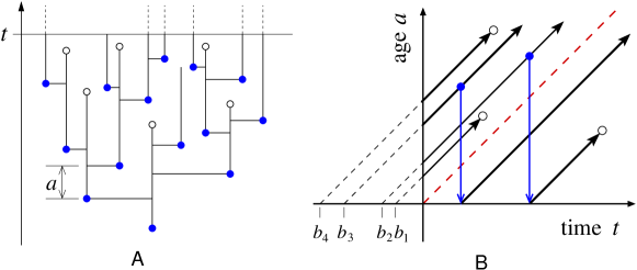
Figure 1: (A) A simple age-dependent birth-death process. Each parent gives birth with an age-dependent rate $\beta_{n}(a)$, which may also depend on the total population size $n$. Individuals can also die (open circles) at an age- and population-dependent rate $\mu_{n}(a)$. (B) Age trajectories in the upper ($a>t$) octant are connected to those in the lower one ($a<t$) through the birth processes. Individuals that exist at time $t=0$ can be traced back and defined by their time of birth $b_{i}$. Here, the labeling ordered according to increasing age. The pictured trajectories define characteristics $a_{i}(t)$ that can be used to solve Eq. 12.

We can now describe the fully stochastic aging process in terms of the ordered distribution function $f_{n}({\bf x}_{n};t)$ by using Eqs. 7-11 in Eq. 6 and applying the operator ${\partial\over\partial a_{n}}\cdots{\partial\over\partial a_{2}}{\partial\over\partial a_{1}}$ to find

$$\begin{array}[]{l}\displaystyle{\partial f_{n}({\bf a}_{n};t)\over\partial t}+\sum_{j=1}^{n}{\partial f_{n}({\bf a}_{n};t)\over\partial a_{j}}=-f_{n}({\bf a}_{n};t)\sum_{i=1}^{n}\gamma_{n}(a_{i})+\sum_{i=0}^{n}\int_{a_{i}}^{a_{i+1}}\!\!\!\!\mu_{n+1}(y)f_{n+1}({\bf a}_{i},y,{\bf a}_{i+1,n};t)\mbox{d}y,\end{array}$$ (12)

where $a_{0}\equiv 0$, $a_{n+1}\equiv\infty$, and the total age-dependent transition rate is

$$\gamma_{n}(a_{i})=\beta_{n}(a_{i})+\mu_{n}(a_{i}).$$ (13)

Note that the $a_{1}-$independent source term $J^{+}_{\beta}$ that had contributed to the ordered cumulative (Eq. 6) does not contribute to the bulk equation for $f_{n}({\bf a}_{n};t)$. Rather, it arises in the boundary condition for $f_{n}$, which can be found by setting $a_{1}=0$ in Eq. 6. Since $Q(0,a_{2},\ldots,a_{n};t)=0$ and $J_{\beta}^{+}({\bf a}_{n};t)$ are independent of $a_{1}$, the remaining terms are

$$\int_{0}^{a_{2}}\!\!\mbox{d}x_{2}\cdots\int_{x_{n-1}}^{a_{n}}\!\!\!\!\mbox{d}x_{n}f_{n}(x_{1}=0,{\bf x}_{2,n};t)=J^{+}_{\beta}({\bf a}_{n};t).$$ (14)

Further taking the derivatives ${\partial\over\partial a_{n}}\cdots{\partial\over\partial a_{2}}$ of Eq. 14, we find the boundary condition

$$f_{n}(a_{1}=0,{\bf a}_{2,n};t)=f_{n-1}({\bf a}_{2,n};t)\sum_{i=2}^{n}\beta_{n-1}(a_{i}).$$ (15)

We now consider indistinguishable individuals as described by the density defined in Eq. 4. Equation 12 can then be expressed in terms of $\rho_{n}({\bf a}_{n};t)$: the probability density that if we randomly label individuals, the first one has age between $a_{1}$ and $a_{1}+\mbox{d}a_{1}$, the second has age between $a_{2}$ and $a_{2}+\mbox{d}a_{2}$, and so on. The kinetic equation for $\rho_{n}$ can then be expressed in the form

$$\displaystyle{\partial\rho_{n}({\bf a}_{n};t)\over\partial t}+ \sum_{j=1}^{n}{\partial\rho_{n}({\bf a}_{n};t)\over\partial a_{j}}=-\rho_{n}({\bf a}_{n};t)\sum_{i=1}^{n}\gamma_{n}(a_{i})+(n+1)\!\int_{0}^{\infty}\!\!\mu_{n+1}(y)\rho_{n+1}({\bf a}_{n},y;t)\mbox{d}y,$$ (16)

and the boundary condition becomes

$$\begin{array}[]{l}n\rho_{n}(a_{1},\ldots,a_{\ell}=0,\ldots,a_{n};t)=\rho_{n-1}(a_{1},\ldots,\hat{a}_{\ell},\ldots,a_{n};t)\sum_{i(\neq\ell)=1}^{n}\beta_{n-1}(a_{i}),\end{array}$$ (17)

where the sum precludes the $i=\ell$ term and $\hat{a}_{\ell}$ indicates that the variable $a_{\ell}$ is omitted from the sequence of arguments Zanette (1990). Equation 16 and the boundary conditions of Eq. 17, along with an initial condition $\rho_{n}({\bf a}_{n};t=0)$, fully define the stochastic age-structured birth-death process and is one of our main results. Eq. 16 is analogous to a generalized Boltzmann equation for $n$ particles Zanette (1990); Peters (1998). The evolution operator corresponds to that of free ballistic motion in one dimension corresponding to age. However, instead of particle collisions typically studied in traditional applications of the Boltzmann equation, our problem couples density functions for $n$ particles to those of $n+1$ and $n-1$ (through the boundary condition).

III Solutions and equation hierarchies

Equation 16 defines a set of coupled linear integro-differential equations. We would like to find solutions for $\rho_{n}({\bf a}_{n};t)$ expressed in terms of an initial condition $g_{n}({\bf a}_{n}-t;t=0)$. However, we will see below that the presence of births during the time interval $[0,t]$ prevents a simple solution to Eq. 16 due to interference from the boundary condition in Eq. 17. Instead, we will obtain a solution for $\rho_{n}({\bf a}_{n};t)$ at time $t$ in terms of the distribution $\rho_{n}({\bf a}_{n}-(t-t_{0});t_{0})$ at an earlier time $t_{0}$ selected such that no births occur during the time interval $(t_{0},t]$. That is, if $b_{i}=t-a_{i}$ represents the time of birth of the $i^{\rm th}$ individual (see Fig. 1B), we have the condition $t_{0}\geq b_{i}\,\forall\,i$. The dynamics described by Eq. 16 are then unaffected by the boundary condition (Eq. 17) and can be solved using the characteristics $a_{i}=t-b_{i}$ indexed by individual times of birth $b_{i}$. Note that any individual initially present (at time $t=0$) has a projected negative time of birth. We can then solve $\rho_{n}(t-{\bf b}_{n};t)$ explicitly along each characteristic and then re-express them in terms of ${\bf a}_{n}$, to obtain

$$\rho_{n}({\bf a}_{n};t) =U_{n}({\bf a}_{n};t_{0};t)\rho_{n}({\bf a}_{n}-(t-t_{0});t_{0})+(n+1)\int_{t_{0}}^{t}U_{n}({\bf a}_{n};t^{\prime};t)\left[\int_{0}^{\infty}\!\!\!\mu_{n+1}(y)\rho_{n+1}\mbox{d}y\right]\mbox{d}t^{\prime},$$ (18)

where $\rho_{n+1}\equiv\rho_{n+1}({\bf a}_{n}-(t-t^{\prime}),y;t^{\prime})$ above, and

$$U_{n}({\bf a}_{m};t^{\prime};t) =\exp\left[-\sum_{i=1}^{m}\int_{t^{\prime}}^{t}\!\gamma_{n}(a_{i}-(t-s))\mbox{d}s\right]\equiv U_{n}^{-1}({\bf a}_{m};t_{0};t^{\prime})U_{n}({\bf a}_{m};t_{0};t)$$ (19)

is the propagator for any set of $m\leq n$ individuals from time $t^{\prime}$ to $t$.

In the case of a pure death process where no births occur ($\beta_{n}=0$), allowing us to set $t_{0}=0$. A complete solution can be found through successive iteration of Eq. 18. We further simplify matters by assuming an initial condition that factorizes into an initial total number distribution $\rho(n)$ and common initial age probability densities $g(a)$: $\rho_{n}({\bf a}_{n}-t;0)=\rho(n)\prod\limits_{i=1}^{n}g(a_{i}-t)$. If we further assume a death rate $\mu_{n}(a)=\mu(a)$ that is independent of population size, Eq. 18 can be solved, after some algebra, to yield

$$\rho_{n}({\bf a}_{n};t)= U({\bf a}_{n};0;t)\prod\limits_{i=1}^{n}g(a_{i}-t)\displaystyle\sum\limits_{k=0}^{\infty}{n+k\choose k}\rho(n+k)\left[\int\limits_{0}^{t}g(y-s)\int\limits_{s}^{\infty}U(y;0;s)\mu(y)\mbox{d}y\mbox{d}s\right]^{k}.$$ (20)

For a pure birth process where $\mu_{n}=0$, the second integral term in Eq. 18 disappears. In this case, we must use the boundary condition (Eq. 17) to successively bootstrap the solution by applying the propagator $U$ between birth times. Assume a starting time $t=0$ with an initial condition consisting of $m$ individuals with corresponding ages $a>t$. The symmetry of $\rho_{n}({\bf a}_{n};t)$ and $U_{n}({\bf a}_{n};t^{\prime};t)$ implies that, without loss of generality, ages can be arranged in decreasing order: $a_{1}>a_{2}>\ldots>a_{m}>t>a_{m+1}>\ldots>a_{n}$, where the youngest was born most recently at time $t-a_{n}>0$. If we select $t_{0}$ to be the moment of birth at time $b_{n}=t-a_{n}$ of the most recently born ($n^{\rm th}$) individual, the density over all individuals is propagated forward according to

$$\rho_{n}({\bf a}_{n};t)=U_{n}({\bf a}_{n};b_{n};t)\rho_{n}(\{{\bf a}_{n-1}-a_{n},0\};t-a_{n}),$$ (21)

where $\rho_{n}(\{{\bf a}_{n-1}-a_{n},0\};t-a_{n})$ is the initial condition immediately after the birth of the $n^{\rm th}$ individual and can be related to $\rho_{n-1}$ through the boundary condition in Eq. 17. The density function thus obeys

$$\rho_{n}({\bf a}_{n};t)= \frac{1}{n}U_{n}({\bf a}_{n};b_{n};t)\rho_{n-1}({\bf a}_{n-1}-a_{n};t-a_{n})\sum_{i=1}^{n-1}\beta_{n-1}(a_{i}-a_{n}).$$ (22)

Eq. 22 can then be iterated back to $t=0$ to find the solution for randomly selected individuals. For the case in which $\gamma_{n}=\gamma$ is independent of the population size, the propagator can be separated into a product across individuals. If $\beta_{n}=\beta$ is also independent of $n$, the solution takes the simple form

$$\rho_{n}({\bf a}_{n};t)= g_{m}({\bf a}_{m}-t)U({\bf a}_{m};0;t){m!\over n!}\!\!\!\prod_{k=m+1}^{n}U(a_{k};b_{k};t)\sum_{\ell=1}^{k-1}\beta(a_{\ell}-a_{k}),$$ (23)

where $b_{k}=t-a_{k}$ and $g_{m}$ is the initial distribution of ages for the $m$ individuals born before $t=0$.

The above solutions for $\rho_{n}({\bf a}_{n};t)$ allow us to explicitly compare differences between the fully stochastic theory and the deterministic McKendrick-von Foerster model. As an example, consider the expected number of individuals at time $t$ that have age between $0$ and $a$,

$$P(a,t)=\int_{0}^{a}\!\!\rho(y,t)\mbox{d}y,$$ (24)

where $\rho(y,t)$ is found from Eqs. 1 and 2. We wish to compare this quantity with the probability $P_{m}(a,t)$ that there are $m$ individuals at time $t$ with age between $0$ and $a$. The probability $P_{m}(n,a,t)$ that there are $n$ total individuals of which exactly $m$ have age between $0$ and $a$ can be constructed from our fully stochastic theory via

$$P_{m}(n,a,t)={n\choose m}\prod_{j=1}^{m}\int_{0}^{a}\mbox{d}a_{j}\!\!\!\prod_{\ell=m+1}^{n}\!\!\!\int_{a}^{\infty}\!\!\!\!\mbox{d}a_{\ell}\,\rho_{n}({\bf a}_{n};t).$$ (25)

The marginal probability $P_{m}(a,t)$ is then found by summing over $n\geq m$:

$$P_{m}(a,t)=\sum_{n=m}^{\infty}P_{m}(n,a,t).$$ (26)

The comparison can be made more explicit by considering simple cases such as an age-independent birth-only process with fixed birth rate $\beta$. If the process starts with precisely $N$ individuals, standard methods Iannelli (1995); Webb (2008) yields a simple solution of the McKendrick-von Foerster equation which when used in Eq. 24 gives $P(a<t;t)=Ne^{\beta t}\left(1-e^{-\beta a}\right)$. Substituting the pure birth solution of Eq. 23 into Eqs. 25 and 26 yields

$$P_{m}(a,t)={m+N-1\choose m}\frac{e^{-N\beta t}\left(1-e^{-\beta a}\right)^{m}}{\left(1-e^{-\beta a}+e^{-\beta t}\right)^{m+N}}.$$ (27)

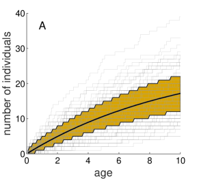
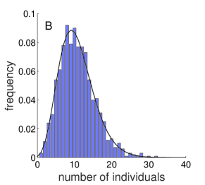
Figure 2: Comparison of $P(a,t)$ (Eq. 24) derived from the McKendrick-von Foerster equation with $P_{m}(a,t)$ of a fully stochastic pure birth process with constant $\beta=0.1$. We start with $N=10$ individuals and analyze our quantities at time $t=10$ for ages $a<t$. (A) Each of the 100 grey lines count the number of individuals younger than age $a$ in one simulation. The solid black curve indicates the deterministic (McKendrick-von Foerster) solution $P(a,t)=\int_{0}^{a}\rho(y,t)\mbox{d}y$, which can also be obtained through $P(a,t)=\sum_{m=1}^{\infty}mP_{m}(a,t)$. The shaded region represents the inter-quartile range of $P_{m}(a,t)$. (B) Distribution constructed from 1000 simulations (bars) and theoretical distribution $P_{m}(a=5,t=10)$ (black curve).

In Fig. 2A we compare the expected value $P(a,t)$ derived from solutions to the McKendrick-von Foerster equation with stochastic simulations that sample the stochastic result $P_{m}(a,t)$. The fully stochastic nature of the process is clearly shown by the spread of the population about the expected value. Fig. 2B plots the corresponding number distribution $P_{m}(5,10)$.

Finally, to connect our general kinetic theory with statistically-reduced (and deterministic) descriptions, we consider reduced $k-$dimensional distribution functions defined by integrating $\rho_{n}({\bf a}_{n};t)$ over $n-k$ age variables:

$$\rho_{n}^{(k)}({\bf a}_{k};t)\equiv\int_{0}^{\infty}\!\mbox{d}a_{k+1}\ldots\int_{0}^{\infty}\!\mbox{d}a_{n}\,\rho_{n}({\bf a}_{n};t).$$ (28)

The symmetry properties of $\rho_{n}({\bf a}_{n};t)$ indicate that it is immaterial which of the $n-k$ age variables are integrated out. If we integrate Eq. 16 over all ages ($k=0$), and assume $\rho_{n}^{(1)}(a=\infty;t)=0$, we find

$${\partial\rho_{n}^{(0)}(t)\over\partial t}= n\rho_{n}^{(1)}(a=0;t)-n\int_{0}^{\infty}\!\!\!\gamma_{n}(y)\rho_{n}^{(1)}(y;t)\mbox{d}y+(n+1)\int_{0}^{\infty}\!\!\!\mu_{n+1}(y)\rho_{n+1}^{(1)}(y;t)\mbox{d}y.$$ (29)

Furthermore, integrating Eq. 17 over $a_{i\neq\ell}$ yields $n\rho_{n}^{(1)}(a=0;t)=(n-1)\int_{0}^{\infty}\beta_{n-1}(y)\rho_{n-1}^{(1)}(y;t)\mbox{d}y$. Thus, Eq. 29 can be written in the form

$$\displaystyle{\partial\rho_{n}^{(0)}(t)\over\partial t}= (n-1)\int_{0}^{\infty}\beta_{n-1}(y)\rho_{n-1}^{(1)}(y;t)\mbox{d}y-n\int_{0}^{\infty}(\beta_{n}(y)+\mu_{n}(y))\rho_{n}^{(1)}(y;t)\mbox{d}y+(n+1)\int_{0}^{\infty}\!\mu_{n+1}(y)\rho_{n+1}^{(1)}(y;t)\mbox{d}y.$$ (30)

Eq. 30 describes the evolution of the probability $\rho_{n}^{(0)}(t)$ that the system contains $n$ individuals at time $t$ and it contains the single-particle marginal density $\rho_{n}^{(1)}(y;t)$. Upon deriving equations for $\rho_{n}^{(1)}(y;t)$, one would find that they depend on $\rho_{n}^{(2)}(y_{1},y_{2};t)$, and so on. Therefore, the marginal probability densities form a hierarchy of equations, as is typically seen in classic settings such as the kinetic theory of gases McQuarrie (2000) and the statistical theory of turbulence Frisch (1995). Note that if the birth and death rates $\beta_{n}$ and $\mu_{n}$ are age-independent, they are constants with respect to the integral and Eq. 30 reduces to the familiar constant birth and death rate master equation for the simple birth-death process:

$${\partial\rho_{n}^{(0)}(t)\over\partial t}= (n-1)\beta_{n-1}\rho_{n-1}^{(0)}(t)-n(\beta_{n}+\mu_{n})\rho_{n}^{(0)}(t)+(n+1)\mu_{n+1}\rho_{n+1}^{(0)}(t),$$ (31)

where $\rho_{n}^{(0)}(t)$ is the probability the system contains $n$ individuals at time $t$, regardless of their ages.

In general, integration of Eq. 16 over $n-k\geq 0$ age variables leaves $k$ remaining independent age variables. The resulting kinetic equation for $\rho_{n}^{(k)}({\bf a}_{k};t)$ involves both $\rho_{n+1}^{(k+1)}({\bf a}_{k},y;t)$ and boundary terms $\rho_{n}^{(k+1)}({\bf a}_{k},a_{k+1}=0;t)$. These boundary terms can be eliminated by using the result obtained from integration of the boundary condition (Eq. 17) over $n-k-1$ age variables. By exploiting the symmetry properties of the marginals $\rho_{n}^{(k)}$, we find

$$\displaystyle{\partial\rho_{n}^{(k)}(t)\over\partial t}+\sum_{i=1}^{k}{\partial\rho_{n}^{(k)}({\bf a}_{k};t)\over\partial a_{i}}= +\left({n-k\over n}\right)\rho_{n-1}^{(k)}({\bf a}_{k};t)\sum_{i=1}^{k}\beta_{n-1}(a_{i})+{(n-k)(n-k-1)\over n}\int_{0}^{\infty}\beta_{n-1}(y)\rho_{n-1}^{(k+1)}({\bf a}_{k},y;t)\mbox{d}y$$

$$\displaystyle-\rho_{n}^{(k)}({\bf a}_{k};t)\sum_{i=1}^{k}\gamma_{n}(a_{i})-(n-k)\int_{0}^{\infty}\gamma_{n}(y)\rho_{n}^{(k+1)}({\bf a}_{k},y;t)\mbox{d}y$$ (32)

$$\displaystyle+(n+1)\int_{0}^{\infty}\mu_{n+1}(y)\rho_{n+1}^{(k+1)}({\bf a}_{k},y;t)\mbox{d}y.$$

Each function $\rho_{n}^{(k)}$ in the hierarchy not only depends on the functions in the $n\pm 1$ subspace, but is connected to functions with $k+1$ and $k-1$ variables. The latter coupling arises through the boundary condition for $\rho_{n}^{(k)}$ which involves densities $\rho_{n}^{(k-1)}$. As with similar equations in physics, the hierarchy of equations cannot be generally solved, and either factorization approximations or truncation (such as moment closure) must be used.

We now show that the $k=1$ equation explicitly leads to the classic McKendrick-von Foerster equation and its associated boundary condition. For $k=1$, $\rho_{n}^{(1)}(a;t)\mbox{d}a$ is the probability that there are $n$ individuals and that if one is randomly chosen, it will have age between $a$ and $a+\mbox{d}a$. Therefore, the probability that we have $n$ individuals of which any one has age between $a$ and $a+\mbox{d}a$ is $n\rho_{n}^{(1)}(a;t)\mbox{d}a$. Summing over all possible population sizes $n\geq 1$ gives us the probability $\rho(a,t)\mbox{d}a$ that the system contains an individual with age between $a$ and $a+\mbox{d}a$:

$$\rho(a,t)\equiv\sum_{n=0}^{\infty}n\rho_{n}^{(1)}(a;t).$$ (33)

Multiplying Eq. III (with $k=1$) by $n$ and summing over all positive integers $n$, we find after carefully cancelling like terms

$${\partial\rho(a,t)\over\partial t}+{\partial\rho(a,t)\over\partial a}=-\sum_{n=1}^{\infty}n\mu_{n}(a)\rho_{n}^{(1)}(a;t).$$ (34)

Equation 34 generalizes the McKendrick-von Foerster model to allow for population-dependent death rates, but does not reduce to the simple form shown in Eq. 1. Population-dependent effects in equation for $\rho(a,t)$ requires requires knowing the “single-particle” density function $\rho_{n}^{(1)}(a;t)$ and subsequently all higher order distribution functions.

A boundary condition is naturally recovered by integrating over all ages but $a_{\ell}$ in Eq. 17 and summing over all $n$:

$$\sum_{n=1}^{\infty}n\rho_{n}^{(1)}(a=0;t) \equiv\rho(a=0,t)=\sum_{n=2}^{\infty}(n-1)\!\int_{0}^{\infty}\!\!\!\beta_{n-1}(y)\rho_{n-1}^{(1)}(y;t)\mbox{d}y.$$ (35)

These equations show that the McKendrick-von Foerster equation is recovered only if both $\mu_{n}(a)=\mu(a)$ and $\beta_{n}(a)=\beta(a)$ are independent of population size. In this case, $\mu(a)$ can be pulled out of the sum in Eq. 34 and $\sum_{n=1}^{\infty}n\mu_{n}(a)\rho_{n}^{(1)}(a;t)=\mu(a)\rho(a,t)$. Similarly, $\int_{0}^{\infty}\beta(y)\left[\sum_{n=2}^{\infty}(n-1)\rho_{n-1}^{(1)}(y;t)\right]\mbox{d}y=\int_{0}^{\infty}\beta(y)\rho(y,t)\mbox{d}y$, which is the simple boundary condition associated with the classic McKendrick-von Foerster model. This derivation clearly shows that population-dependent birth and death rates cannot be readily incorporated into an age-dependent model, even one that is deterministic, without considering the hierarchy of population densities.

IV Discussion and conclusions

We have developed a complete kinetic theory for age-structured birth-death processes. To stochastically describe the age structure of a population requires a higher dimensional probability density. The evolution of this high-dimensional probability density mirrors that found in the Boltzmann equation for one-dimensional, ballistic, noninteracting gas dynamics. However, one crucial difference is that the number of individuals can increase or decrease according to the age-dependent birth and death rates. Thus, the dynamics are determined by a phase-space-conserving Liouville operator so long as the number of individuals does not change McQuarrie (2000). Once an individual is born or dies, the system jumps to another manifold in a higher or lower dimensional phase-space, immediately after which conserved dynamics resume until the next birth or death event. Such variable number dynamics share similarities with the kinetic theory of chemically reacting gases Rossani and Spiga (1999).

Our main mathematical results are Eqs. 16 and 17. These equations show that birth-death dynamics couple densities associated with different numbers $n$ and describes the process in terms of ballistically moving particles all moving with unit velocity in the age “direction.” The individual particles can die at rates that depend on their distance from their origin (birth). Particles can also give birth at rates dependent on their age. The injection of newborns at the origin (zero age) is described by the boundary condition (Eq. 17).

One important advantage of our approach is that it provides a natural framework for incorporating both age- and population-dependent birth and death rates into a stochastic description, which has thus far not been possible with other approaches. In general, our kinetic equations need to be solved numerically; however, we found analytic expressions for $\rho_{n}({\bf a}_{n};t)$ when either birth or death vanishes and the other is independent of population. Furthermore, we define marginal density functions and develop a hierarchy of equations analogous to the BBGKY hierarchy (Eq. III). These equations for the marginal densities allow one to construct any desired statistical measure of the process and are also part of our main results. We explicitly showed how a zeroth order equation leads to the equation for the marginal probability of observing $n$ individuals in the standard age-independent birth-death processes (Eq. 31) Allen (2003). The first-order equation is also used to derive a hybrid equation for the mean density $\rho(a,t)$ that involves the single-particle density function $\rho_{n}^{(1)}(a;t)$ (which ultimately depends on higher-dimensional densities $\rho_{n}^{(k>1)}({\bf a}_{k};t)$ through the hierarchy). Only when death is independent of population does the theory reduce to the deterministic McKendrick-von Foerster equation (Eq. 34) and the associated boundary condition (Eq. 35).

Extensions of our high-dimensional age-structured kinetic theory to more complex birth-death mechanisms such as sexual reproduction and renewal/branching processes can be straightforwardly investigated. The simple birth-death process we analyzed allows for the birth of only a single age-zero daughter from a parent at a time. We note that the Bellman-Harris process described via generating functions Jagers (1968); Shonkwiler (1980) (which can describe age-dependent death and branching, but cannot be used to model population-dependent dynamics) assumes self-renewal at each branching event. That is, two (or more) daughters of zero age are simultaneously produced from a parent. Such differences in the underlying birth process can lead to qualitative differences in important statistical measures beyond mean-field, such as first passage times Chou and Wang (2015). The branching/renewal process, as well as sexual reproduction, requires nontrivial extensions of our kinetic theory and will be explored in a future investigation.

V Acknowledgements

This research was supported in part at KITP by the National Science Foundation under Grant No. PHY11-25915. TC is also supported by the NIH through grant R56 HL126544 and the Army Research Office through grant W911NF-14-1-0472.

References

- Keyfitz and Caswell (2005) N. Keyfitz and H. Caswell, Applied Mathematical Demography, 3rd Ed. (Springer, New York, NY, 2005).
- Ayati (2007) B. P. Ayati, Appl. Math. Lett. 20, 913 (2007).
- Stukalin et al. (2013) E. B. Stukalin, I. Aifuwa, J. S. Kim, D. Wirtz, and S. X. Sun, Interface 10, 20130325 (2013).
- Roshan et al. (2014) A. Roshan, P. H. Jones, and C. D. Greenman, J. Roy. Soc. Interface 11, 20140654 (2014).
- Qu et al. (2003) Z. Qu, W. R. MacLellan, and J. N. Weiss, Biophysical Journal 85, 3600 (2003).
- Weber et al. (2014) T. S. Weber, I. Jaehnert, C. Schichor, M. Or-Guil, and J. Carneiro, PLoS Comput. Biol. 10, e1003616 (2014).
- Oh et al. (2014) J. Oh, Y. D. Lee, and A. J. Wagers, Nature Medicine 20, 870 (2014).
- McKendrick (1926) A. G. McKendrick, Proc. Edinburgh Math. Soc. 44, 98 (1926).
- Keyfitz and Keyfitz (1997) B. L. Keyfitz and N. Keyfitz, Mathl. Comput. Modelling 26, 1 (1997).
- von Foerster (1959) H. von Foerster, Some remarks on changing populations in The Kinetics of Cell Proliferation (Springer, 1959).
- Gurtin and MacCamy (1974) M. E. Gurtin and R. C. MacCamy, Arch. Rational Mech. Anal pp. 281–300 (1974).
- Gurtin and MacCamy (1979) M. E. Gurtin and R. C. MacCamy, Math. Biosci pp. 199–211 (1979).
- Iannelli (1995) M. Iannelli, Mathematical theory of age-structured population dynamics, Applied Mathematics Monographs (Giardini editori e stampatori, 1995).
- Webb (2008) G. F. Webb, in Structured population models in biology and epidemiology, edited by P. Magal and S. Ruan (Springer, Berlin, Heidelberg, 2008), pp. 1–49.
- Kampen (2011) N. G. V. Kampen, Stochastic Processes in Physics and Chemistry, North-Holland Personal Library (Elsevier Science, 2011).
- Chou and D’Orsogna (2014) T. Chou and M. R. D’Orsogna, in First-Passage Phenomena and Their Applications, edited by R. Metzler, G. Oshanin, and S. Redner (World Scientific, Singapore, 2014), pp. 306–345.
- Bellman and Harris (1948) R. Bellman and T. E. Harris, Proc. Natl. Acad. Sci. USA 34, 601 (1948).
- Reid (1953) A. T. Reid, Bull. Math. Biophysics 15, 361 (1953).
- Jagers (1968) P. Jagers, Theory of Probability and its Applications 13, 225 (1968).
- Shonkwiler (1980) R. Shonkwiler, Comp. & Maths. with Appls. 6, 289 (1980).
- Chou and Wang (2015) T. Chou and Y. Wang, J. Theor. Biol. 372, 65 (2015).
- Kendall (1948) D. G. Kendall, Ann. Math. Statist. 19, 1 (1948).
- Allen (2003) L. J. S. Allen, An introduction to Stochastic Processes with Application to Biology (Pearson Prentice Hall, 2003).
- Chowdhury (1998) M. Chowdhury, A stochastic age-structured population model, Master’s thesis, Texas Tech University, Lubbock, TX (1998).
- Li et al. (2009) R. Li, P.-K. Leung, and W.-K. Pang, J. Comp. Appl. Math. 233, 1046 (2009).
- Getz (1984) W. M. Getz, Mathematical Biosci. 69, 11 (1984).
- Cohen et al. (1983) J. E. Cohen, S. W. Christensen, and C. P. Goodyear, Can. J. Fish. Aquat. Sci. 40, 2170 (1983).
- Leslie (1945) P. H. Leslie, Biometrika 33, 183 (1945).
- Leslie (1948) P. H. Leslie, Biometrika 35, 213 (1948).
- Lande and Orzack (1988) R. Lande and S. H. Orzack, Proc. Natl. Acad. Sci. USA 85, 7418 (1988).
- Engen et al. (2005) S. Engen, R. Lande, and B.-E. Saether, Genetics 170, 941 (2005).
- Pollard (1966) J. H. Pollard, Biometrika 53, 397 (1966).
- McQuarrie (2000) D. A. McQuarrie, Statistical Mechanics (University Science Books, 2000).
- Zanette (1990) D. H. Zanette, Physica A 162, 414 (1990).
- Peters (1998) M. H. Peters, arXiv:physics/9809039v2 (1998).
- Frisch (1995) U. Frisch, Turbulence (Cambridge University Press, Cambridge, UK, 1995).
- Rossani and Spiga (1999) A. Rossani and G. Spiga, Physica A: Statistical Mechanics and its Applications 272(3-4), 563 (1999).