Frequency-Domain Analysis of Nonlinear and Linear Integrators

Abstract

In this paper, frequency-domain analysis based on frequency sweep method is presented for a nonlinear double integrator and a new linear integrator. All the two types of integrators can estimate the onefold and double integrals of a signal synchronously. With respect to the linear double integrator, the nonlinear integrator has better estimation performance and stronger robustness. Importantly, the integrator parameters can be regulated from the frequency-domain analysis.

I Introduction

This paper focuses on the frequency-domain analysis of two types of integrators, which can estimate the onefold and double integrals of a signal synchronously.

Integrals are important components in almost all engineering applications. The problem of double integral is that of estimating the number $I_{2}\left(a\right)=\int_{0}^{t}\int_{0}^{s}a\left(\sigma\right)d\sigma d\tau$ with $\left[0,t\right]$ a finite time interval. Obtaining the double integral of a signal is crucial for many kinds of systems, especially for Inertial Navigation System (INS).

The usual observers or differentiators [1]-[4] can estimate the derivatives of the signal, but not its multiple integrals. There are several linear approximated methods to estimate onefold integral [5-8]: Romberg integration, Gaussian quadrature, extended Simpson’s rule, fractional-order integrator. In all of the aforementioned studies, there is no stability analysis. Furthermore, they are easily disturbed by stochastic noise (especially non-white noise), and the drift phenomena occur in such systems. In [9], a fractional-order integrator is proposed to approximate the irrational fractional-order integrator $1/s^{m}$. However, the condition of $0<m<1$ limits the application of the fractional-order integrator. Recently years, Kalman filter is used to handle the separation of probabilistic noise and to estimate the position and velocity from the acceleration measurement [10]-[12]. However, for Kalman filter, it is assumed that the process noise covariance and measurement noise covariance are zero-mean Gaussian distributed, and the process noise covariance is uncorrelated to the estimation error. These assumptions are different from the real noise in signal. The inaccurate noise information in sensed accelerations may lead to the estimate drifts of position and velocity.

In [13], a nonlinear double integrator was presented based on finite-time stability [14, 15]. The proposed double integrator can estimate the onefold and double integrals of a signal synchronously, and the stability and robustness in time domain were analyzed. The merits of the presented double integrator include its finite-time stability, ease of parameters selection, sufficient stochastic noise rejection and almost no drift phenomenon. The theoretical results are confirmed by an experiment on a quadrotor aircraft to estimate the position and velocity from the acceleration measurement. The nonlinear double integrator leads to perform rejection of low-level persistent disturbances. However, no robustness for high-frequency noise is analyzed, i.e., no frequency-domain analysis on the effect of high-frequency noise is considered. In fact, stochastic high-frequency noise exist in almost all signals. Therefore, with respect to the ability of rejecting of low-level persistent disturbances, the strong robustness of reducing high-frequency noise is also necessary. And the parameters selection based on frequency-domain analysis is required.

In this paper, based on singular perturbation technique [16, 17], a linear double integrator is presented to estimate the onefold and double integrals of a signal synchronously. Moreover, using frequency sweep method, frequency-domain analysis is presented for the nonlinear double integrator in [13] and the linear integrator. From the frequency-domain analysis, comparing to the linear double integrator, the nonlinear integrator has the better estimation performance and stronger robustness. Also the observer parameters are more easily to be chosen from the frequency-domain analysis with respect to the analysis in time domain.

II Nonlinear and linear double integrators

II-A Nonlinear double integrator

A nonlinear double integrator has been presented in [13], i.e., for system

$$\dot{x}_{1} = x_{2};\dot{x}_{2}=x_{3};$$

$$\varepsilon^{4}\dot{x}_{3} = -\sum\limits_{{i=1}}^{{2}}k_{i}\left|\varepsilon^{i}x_{i}\right|^{\alpha_{i}}sign\left(x_{i}\right)$$ (1)

$$-k_{3}\left|x_{3}-a\left(t\right)\right|^{\alpha_{3}}sign\left(x_{3}-a\left(t\right)\right)$$

if input signal $a\left(t\right)$ is the continuous and first-order derivable, then there exist $\gamma>1$ and $\Gamma>0$, such that, for $t\geq\varepsilon\Gamma\left(\Xi(\varepsilon)e\left({0}\right)\right)$,

$$\left|x_{i}-a_{i}\left(t\right)\right|\leq L\varepsilon^{\alpha_{1}\gamma-i},i=1,2,3$$ (2)

where $a_{1}\left(t\right)=\int_{0}^{t}\int_{0}^{\sigma_{2}}a\left(\sigma_{1}\right)d\sigma_{1}d\sigma_{2}$, $a_{2}\left(t\right)=\int_{0}^{t}a\left(\sigma_{1}\right)d\sigma_{1}$; $x_{1}\left(0\right)=a_{1}\left(0\right)$, $x_{2}\left(0\right)=a_{2}\left(0\right)$, $x_{3}\left(0\right)=a_{3}\left(0\right)$; $\varepsilon\in\left(0,1\right)$ is the perturbation parameter; $L$ is some positive constant; $\gamma=(1-\beta)/\beta>1$, and $\beta\in\left(0,\alpha_{1}/(\alpha_{1}+4)\right)$; $\alpha_{1},\alpha_{2},\alpha_{3}$ satisfy:

$$\alpha_{3}\in(0,1),\alpha_{2}=\frac{\alpha_{3}}{2-\alpha_{3}},\alpha_{1}=\frac{\alpha_{3}}{3-2\alpha_{3}}$$ (3)

$k_{1},k_{2},k_{3}>0$ are selected such that

$$k_{1}>0,k_{3}>0,k_{2}>\varepsilon^{3\alpha_{3}}\frac{k_{1}}{k_{3}}$$ (4)

$e_{i}=x_{i}-a_{i}\left(t\right)$, $i=1,2,3$; $e=[\begin{array}[]{ccc}e_{1}&e_{2}&e_{3}\end{array}]^{{T}}$; $\Xi(\varepsilon)=diag\{\varepsilon,\varepsilon^{2},\varepsilon^{3}\}$.

In nonlinear double integrator (1), $x_{3}$ tracks the input signal $a(t)$, $x_{2}$ and $x_{1}$ estimate the onefold and double integrals of signal $a(t)$, respectively. From Theorem 1 in [13], nonlinear double integrator (1) leads to perform rejection of low-level persistent disturbances. However, no frequency-domain analysis on the effect of high-frequency noise is considered. In fact, high-frequency noise exist in almost all signals. Therefore, the frequency-domain analysis for the nonlinear double integrator is inevitable.

As we know, a linear system is easy to perform frequency-domain analysis with respect to nonlinear one. In the following, based on the design of nonlinear double integrator, a simple linear double integrator will be designed (when $\alpha_{3}=1$), and Theorem 1 is presented as follow.

II-B Linear double integrator

Theorem 1: For system

$$\dot{x}_{1} = x_{2};\dot{x}_{2}=x_{3};$$

$$\varepsilon^{4}\dot{x}_{3} = -k_{1}\varepsilon x_{1}-k_{2}\varepsilon^{2}x_{2}-k_{3}\left(x_{3}-a\left(t\right)\right)$$ (5)

if input signal $a\left(t\right)$ is continuous, integrable and first-order derivable, then

$$\underset{\varepsilon\rightarrow 0}{\lim}x_{i}=a_{i}\left(t\right),i=1,2,3$$ (6)

where $a_{1}\left(t\right)=\int_{0}^{t}\int_{0}^{\tau}a\left(s\right)dsd\tau$, $a_{2}\left(t\right)=\int_{0}^{t}a\left(\tau\right)$, $a_{3}\left(t\right)=a\left(t\right)$; $x_{i}\left(0\right)=a_{i}\left(0\right)$, $i=1,2$; $\varepsilon\in\left(0,1\right)$ is the perturbation parameter; $k_{1},k_{2},k_{3}>0$ are selected such that

$$k_{1}>0,k_{3}>0,k_{2}>\varepsilon^{3}\frac{k_{1}}{k_{3}}$$ (7)

In linear double integrator (5), $x_{3}$ tracks the input signal $a(t)$, $x_{2}$ and $x_{1}$ estimate the onefold and double integrals of signal $a(t)$, respectively.

Proof of Theorem 1: The Laplace transformation of Eq. (5) can be obtained as follow:

$$sX_{1}\left(s\right) = X_{2}\left(s\right);sX_{2}\left(s\right)=X_{3}\left(s\right);$$

$$s\varepsilon^{4}X_{3}\left(s\right) = -\sum\limits_{{i=1}}^{{2}}k_{i}\varepsilon^{i}X_{i}\left(s\right)$$ (8)

$$-k_{3}\left(X_{3}\left(s\right)-A\left(s\right)\right)$$

where $X_{i}\left(s\right)$ and $A\left(s\right)$ denote the Laplace transformations of $x_{i}$ and $a\left(t\right)$, respectively, and $s$ denotes Laplace operator. From (8), we obtain

$$X_{i}\left(s\right)=\frac{X_{j}\left(s\right)}{s^{j-i}},i=1,2,3,j\in\left\{1,2,3\right\}$$ (9)

Therefore, Eq. (8) can be written as

$$s^{3-j+1}\varepsilon^{4}X_{j}\left(s\right) = -\sum\limits_{{i=1}}^{{2}}k_{i}\varepsilon^{i}\frac{X_{j}\left(s\right)}{s^{j-i}}$$ (10)

$$-k_{3}\left(\frac{X_{j}\left(s\right)}{s^{j-3}}-A\left(s\right)\right)$$

Then, it follows that

$$\frac{X_{j}\left(s\right)}{A\left(s\right)}=\frac{k_{3}}{s^{3-j+1}\varepsilon^{4}+\sum\limits_{{i=1}}^{{2}}\frac{k_{i}\varepsilon^{i}}{s^{j-i}}+\frac{k_{3}}{s^{j-3}}}$$ (11)

i.e.,

$$\frac{X_{j}\left(s\right)}{A\left(s\right)}=\frac{s^{j-1}k_{3}}{s^{3}\varepsilon^{4}+\sum\limits_{{i=1}}^{{2}}s^{i-1}k_{i}\varepsilon^{i}+s^{2}k_{3}}$$ (12)

Therefore, we obtain

$$\underset{\varepsilon\rightarrow 0}{\lim}\frac{X_{j}\left(s\right)}{A\left(s\right)}=s^{j-3}$$ (13)

where $j\in\left\{1,2,3\right\}$. It means that $x_{i}$ approximates $a_{i}\left(t\right)$ for $1\leq i\leq 3$.

Furthermore, the denominator of Equation (12) is required to be Hurwitz, i.e., polynomial $s^{3}+\frac{k_{3}/\varepsilon^{3}}{\varepsilon}s^{2}+\frac{k_{2}}{\varepsilon^{2}}s+\frac{k_{1}}{\varepsilon^{3}}$ is Hurwitz. It is equivalent that $s^{3}+\frac{k_{3}}{\varepsilon^{3}}s^{2}+k_{2}s+k_{1}$ should be Hurwitz. For arbitrary $\varepsilon\in\left(0,1\right)$, from the Routh-Hurwitz Stability Criterion, polynomial $s^{3}+\frac{k_{3}}{\varepsilon^{3}}s^{2}+k_{2}s+k_{1}$ is Hurwitz if $k_{1}>0,k_{3}>0,k_{2}>\varepsilon^{3}k_{1}/k_{3}$. This concludes the proof. $\blacksquare$

From Theorem 1, the presented linear double integrator can’t guarantee to perform rejection of high-frequency noise. In fact, the robustness for the effect of high-frequency noise exist. With respect to nonlinear double integrator (1), the advantage of linear double integrator (5) is its simple implementation.

In the next section, the frequency-domain analysis will be presented for the nonlinear and linear double integrators.

III Frequency-domain analysis based on frequency sweep

In a practical problem, high-frequency noises exist in measurement signal $a(t)$. The following analysis concerns the robustness behaviors of the nonlinear and linear double integrators under high-frequency noises.

For the nonlinear double integrator, an extended version of the frequency response method, frequency-sweep method [18, 19], can be used to approximately analyze and predict the nonlinear behaviors of the nonlinear integrator. Even though it is only an approximation method, the desirable properties it inherits from the frequency response method, and the shortage of other, systematic tools for nonlinear integrator analysis, make it an indispensable component of the bag of tools of practicing control engineers. By frequency-sweep method, we can find that the nonlinear double integrator leads to perform precise estimation of integrals and strong rejection of high-frequency noise.

The test of frequency characteristic can be implemented by Bode plot fitting. For linear or nonlinear double integrators (1) or (5), let the input signal be

$$a(t)=A_{m}\sin(\omega t)$$ (14)

where $A_{m}$ and $\omega$ are the amplitude and angular rate of the input signal, respectively. Suppose the output of the double integrator can be expressed as

$$y(t) = A_{f}\sin(\omega t+\varphi)$$ (18)

$$= \left[\begin{array}[]{cc}\sin(\omega t)&\cos(\omega t)\end{array}\right]\left[\begin{array}[]{c}A_{f}\cos\varphi\\ A_{f}\sin\varphi\end{array}\right]$$

where $A_{f}$, $\omega$ and $\varphi$ are the amplitude, angular rate and phase of the output signal, respectively. Let $t=0$, $h$, $2h$, $\cdots$, $nh$, and

$$Y^{T} = \left[\begin{array}[]{cccc}y(0)&y(h)&\cdots&y(nh)\end{array}\right]$$ (20)

$$\Psi^{T} = \left[\begin{array}[]{cccc}\sin(\omega 0)&\sin(\omega h)&\cdots&\sin(\omega nh)\\ \cos(\omega 0)&\cos(\omega h)&\cdots&\cos(\omega nh)\end{array}\right]$$ (23)

$$c_{1} = A_{f}\cos\varphi,c_{2}=A_{f}\sin\varphi$$ (24)

where $h$ is the step size. From (15) and (16), it follows that

$$Y=\Psi\left[\begin{array}[]{cc}c_{1}&c_{2}\end{array}\right]^{T}$$ (25)

From the least square method, $c_{1}$ and $c_{2}$ can be obtained as follow:

$$\left[\begin{array}[]{cc}\hat{c}_{1}&\hat{c}_{2}\end{array}\right]^{T}=(\Psi^{T}\Psi)^{-1}\Psi^{T}Y$$ (26)

For the angular rate $\omega$, the amplitude and phase of the output signal are, respectively, written as

$$\hat{A}_{f}=\sqrt{\hat{c}_{1}^{2}+\hat{c}_{2}^{2}},\hat{\varphi}=\arctan(\hat{c}_{2}/\hat{c}_{1})$$ (27)

Therefore, the amplitude frequency characteristic can be described as

$$\hat{M}=20\lg(\hat{A}_{f}/A_{m})=20\lg(\sqrt{\hat{c}_{1}^{2}+\hat{c}_{2}^{2}}/A_{m})$$ (28)

and the phase frequency characteristic is the phase error between the output and input, and it can be described as

$$\varphi_{e}=\varphi_{out}-\varphi_{in}=\arctan(\hat{c}_{2}/\hat{c}_{1})$$ (29)

The angular frequency sequence $\{\omega_{k}\}$, where $k=1,\cdots,n$, is selected in the interested frequency bandwidth. For each angular frequency the frequency bandwidth, the above frequency-sweep method is adopted to obtain the values of amplitude and phase, respectively. Accordingly, the Bode plots of the frequency-domain characteristic can be described.

In this frequency-domain analysis, $\omega=2\pi f$, where $f=0.1:0.5:100$; $h=0.001$; $k=1:1:50000$. Then input signal is $a(k)=A_{m}\sin(2\pi fkh)$.

In the following, using frequency-sweep method, we will analyze the effects of the observer parameters on the estimate performances and robustness.

III-A Frequency characteristics with different $\varepsilon$ and $\alpha_{3}$

For the nonlinear and linear double integrators (1) and (5), the parameters are selected as follows: $k_{1}=0.1$, $k_{2}=0.1$, $k_{3}=1$; $A_{m}=1$; $\alpha_{3}=\alpha=0.3,0.5,1$, respectively; $R=1/\varepsilon=3,4,5$, respectively. The Bode plots of the frequency-domain characteristics with different $\varepsilon$ and $\alpha_{3}=\alpha$ are described in Figs. 1(a), 1(b) and 1(c), respectively: Fig. 1(a) presents the frequency characteristic of signal tracking; Figs. 1(b) and 1(c) present the frequency characteristics of onefold and double integral estimations, respectively. We can find that high-frequency noise can be reduced sufficiently. Moreover, decreasing parameter $\varepsilon$, the cut-off frequency become larger. The smaller $\varepsilon$ is, the signal in wider frequency bandwidth can be estimated. However, much noise will pass through the observer. On the other hand, increasing parameter $\varepsilon$, the cut-off frequency become smaller, much noise will be rejected.

Importantly, from Figs. 1(a), 1(b) and 1(c), changing parameter $\alpha_{3}\in(0,1]$, the amplitude frequency characteristics almost don’t be affected, but the phase frequency characteristics are affected obviously: when $\alpha_{3}$ approaches to $1$, the phase frequency characteristic curves decay slowly near the cut-off frequency, and phase delay and chattering exist. On the other hand, decreasing parameter $\alpha_{3}\in(0,1)$, the phase frequency characteristic curves decay rapidly at the cut-off frequency. Relatively smaller $\alpha_{3}\in(0,1)$ can obtain more precise estimations and stronger robustness.

III-B Frequency characteristics with the change of $A_{m}$

For nonlinear double integrator (1), the parameters are selected as follows: $\alpha_{3}=0.3$; $R=1/\varepsilon=3$; $k_{1}=0.1$, $k_{2}=0.1$, $k_{3}=1$; $A_{m}=5,1,0.5$, respectively. The Bode plots of the frequency-domain characteristics with the change of $A_{m}$ are described in Figs. 2(a), 2(b) and 2(c), respectively: Fig. 2(a) presents the frequency characteristic of signal tracking; Figs. 2(b) and 2(c) present the frequency characteristics of onefold and double integral estimations, respectively. It is found that, when the magnitude of input signal $A_{m}$ is larger, the cut-off frequency is relatively smaller, and much noise is reduced sufficiently; when the magnitude $A_{m}$ is smaller, the cut-off frequency is relatively larger, and the signal in wider frequency bandwidth can be estimated.

Remark 1: Comparing with ideal integral operators $1/s$ and $1/s^{2}$, not only the double integrators can obtain their estimations precisely, but also the high-frequency noise is reduced sufficiently. Parameter $\varepsilon$ affects the low-pass frequency bandwidth: Decreasing the perturbation parameter $\varepsilon$, the low-pass frequency bandwidth is larger, the estimation precision becomes better, and relatively higher frequency noise can be reduced; on the other hand, increasing perturbation parameter $\varepsilon$, the low-pass frequency bandwidth is smaller, much noise can be reduced sufficiently (See the cases of $R=1/\varepsilon=3,4,5$ in Figure 1, respectively). Parameter $\alpha_{3}\in(0,1]$ affects the decay speed of frequency characteristic curves near the cut-off frequency (See the cases of $\alpha_{3}=\alpha=0.3,0.5,1$ in Figure 1, respectively): Smaller $\alpha_{3}\in(0,1]$ can obtain more precise estimations; Larger $\alpha_{3}\in(0,1]$ can restrain much noise, however, estimation delay phenomena exist.

IV Computational analysis and simulations

In this section, simulation results are presented in order to observe the performances of the nonlinear and linear double integrators. We consider the simulations of the following case: Double integrators for a input signal with high-frequency noise. In the simulations, the function of $-0.1\times 3.14^{2}\times\sin(3.14t)$ is selected as reference signal $a_{03}(t)$. Therefore, $a_{02}=\int_{0}^{t}a_{03}(\sigma)d\sigma=0.1\times 3.14\times\cos(3.14t)$, and $a_{01}=\int_{0}^{t}\int_{0}^{s}a_{03}\left(\sigma\right)d\sigma d\tau=0.1\sin(3.14t)$.

Here, the following high-frequency noise $\delta(t)$ is selected (See the noise in Fig. 3(a)): $0.1\sin(10t)+0.1\cos(10t)+0.05\sin(50t)+0.05\cos(50t)$.

Therefore, the input signal $a(t)=a_{03}(t)+\delta(t)$. From the frequency-domain analysis, the observer parameters can be selected as follows: $R=1/\varepsilon=5$, $k_{1}=0.1$, $k_{2}=0.1$, $k_{3}=1$, $\alpha_{3}=\alpha=0.3$, $\alpha_{2}=\frac{\alpha}{2-\alpha},\alpha_{1}=\frac{\alpha}{3-2\alpha}$; the initial value of the observer is ($x_{1}\left(0\right)=0,x_{2}\left(0\right)=1,x_{3}\left(0\right)=0$). In the double integrators (1) or (5), $x_{3}$ tracks signal $a_{03}(t)$, $x_{2}$ and $x_{1}$ estimate the onefold and double integrals of signal $a_{03}(t)$, respectively.

Signal $a_{03}(t)$ tracking, the onefold and double integral estimations in 20 seconds are presented in Fig. 3. Fig. 3(a) provides signal $a_{03}\left(t\right)$ with stochastic noise. Fig. 3(b) describes $a_{03}(t)$ tracking. Figs. 3(c) and 3(d) present the onefold and double integral estimations, respectively. Figs. 4(a)-4(d) describe the onefold and double integral estimations in 2000 seconds.

From the above simulations, despite the existence of the intensive high-frequency noise, the nonlinear double integrator showed the promising estimation ability and robustness. Furthermore, from Figs. 4(a)-4(d), no drift phenomenon happened in the long-time estimations.

Figs. 5 and 6 describe the estimations of onefold and double integrals by the linear double integrator (5) (when $\alpha_{3}=1$), in 20s and 2000s, respectively. From Figs. 5 and 6, the obvious estimation delay and slow convergence of double integral exist.

V Conclusions

Based on frequency sweep method, frequency-domain analysis is proposed for the nonlinear double integrator and the linear integrator. All the two types of integrators have the strong robustness for the effect of high-frequency noise. Comparing to the linear double integrator, the nonlinear integrator has the better estimation performance and stronger robustness. Importantly, the integrator parameters are easily to be chosen from the frequency-domain analysis with respect to the analysis in time domain.

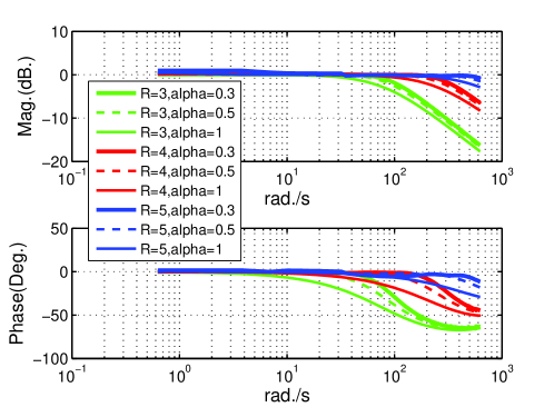
1(a)

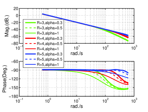
1(b)

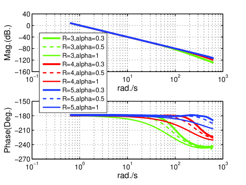
1(c)

Figure 1: Frequency-domain characteristics with different $\varepsilon$ and $\alpha$. 1(a) Signal tracking. 1(b) Onefold integral estimate. 1(c) Double integral estimate.

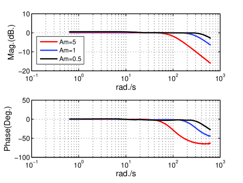
2(a)

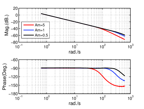
2(b)

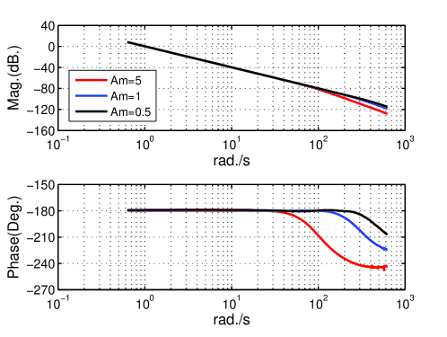
2(c)

Figure 2: Frequency-domain characteristics with the change of $A_{m}$. 2(a) Signal tracking. 2(b) Onefold integral estimate. 2(c) Double integral estimate.

3(a)

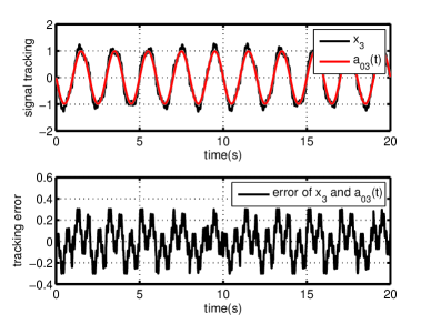
3(b)

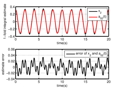
3(c)

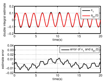
3(d)

Figure 3: Integral estimations in 20s ($\alpha_{3}=0.3$). 3(a) Input signal with noise. 3(b) Signal tracking. 3(c) Onefold integral estimate. 3(d) Double integral estimate.

4(a)

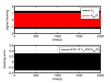
4(b)

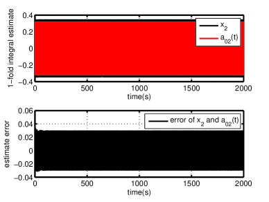
4(c)

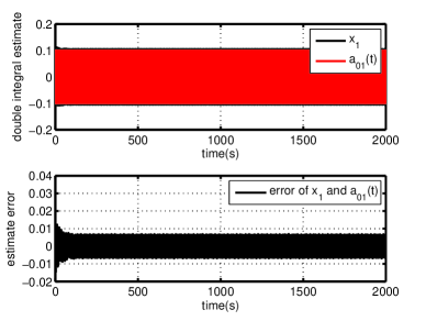
4(d)

Figure 4: Integral estimations in 2000s ($\alpha_{3}=0.3$). 4(a) Input signal with noise. 4(b) Signal tracking. 4(c) Onefold integral estimate. 4(d) Double integral estimate.

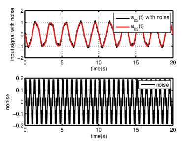
5(a)

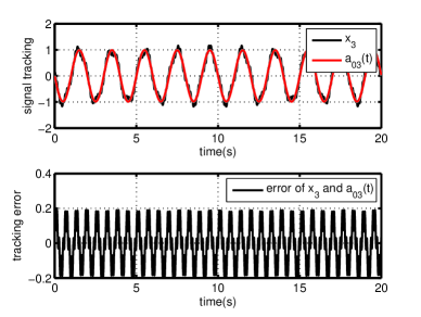
5(b)

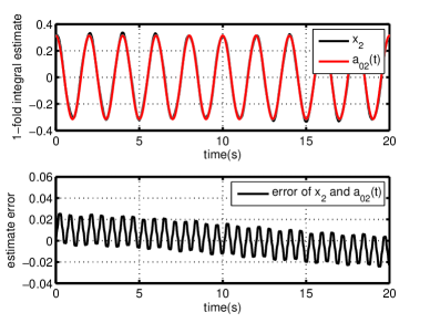
5(c)

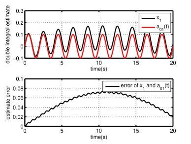
5(d)

Figure 5: Integral estimations in 20s ($\alpha_{3}=1$). 5(a) Input signal with noise. 5(b) Signal tracking. 5(c) Onefold integral estimate. 5(d) Double integral estimate.

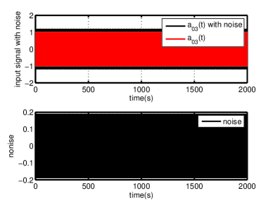
6(a)

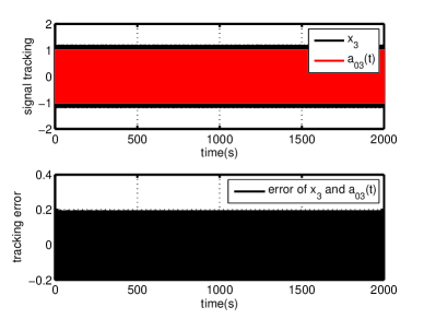
6(b)

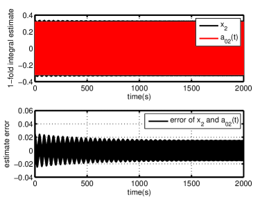
6(c)

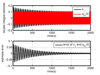
6(d)

Figure 6: Integral estimations in 2000s ($\alpha_{3}=1$). 6(a) Input signal with noise. 6(b) Signal tracking. 6(c) Onefold integral estimate. 6(d) Double integral estimate.