Sentence Directed Video Object Codetection

Abstract

We tackle the problem of video object codetection by leveraging the weak semantic constraint implied by sentences that describe the video content. Unlike most existing work that focuses on codetecting large objects which are usually salient both in size and appearance, we can codetect objects that are small or medium sized. Our method assumes no human pose or depth information such as is required by the most recent state-of-the-art method. We employ weak semantic constraint on the codetection process by pairing the video with sentences. Although the semantic information is usually simple and weak, it can greatly boost the performance of our codetection framework by reducing the search space of the hypothesized object detections. Our experiment demonstrates an average IoU score of 0.423 on a new challenging dataset which contains 15 object classes and 150 videos with 12,509 frames in total, and an average IoU score of 0.373 on a subset of an existing dataset, originally intended for activity recognition, which contains 5 object classes and 75 videos with 8,854 frames in total.

1 Introduction

In this paper, we address the problem of codetecting objects with bounding boxes from a set of videos, without any pretrained object detectors. The codetection problem is typically approached by selecting one out of many object proposals per image or frame that maximizes a combination of the confidence scores associated with the selected proposals and the similarity scores between proposal pairs. While much prior work focuses on codetecting objects in still images (e.g., [7, 25, 39, 42]), little prior work [34, 40, 22, 41, 35] attempts to codetect objects in video. In both lines of work, most [7, 25, 39, 42, 34, 22] assume that the objects to be codetected are salient, both in size and appearance, and located in the center of the field of view. Thus they easily “pop out.” As a result, prior methods succeed with a small number of object proposals in each image or frame. Tang et al. [42] and Joulin et al. [22] used approximately 10 to 20 proposals per image, while Lee and Grauman [25] used 50 proposals per image. Limiting codetection to objects in the center of the field of view allowed Prest et al. [34] to prune the search space by penalizing proposals in contact with the image perimeter. Moreover, under these constraints, the confidence score associated with proposals is a reliable measure of salience and a good indicator of which image regions constitute potential objects [39]. In prior work, the proposal confidence dominates the overall scoring process and the similarity measure only serves to refine the confidence. In contrast, Srikantha and Gall [41] attempt to codetect small to medium sized objects in video, without the above simplifying assumptions. However, in order to search through the larger resulting object proposal space, they avail themselves of human pose and depth information to prune the search space. It should also be noted that all these codetection methods, whether for images or video, codetect only one common object at a time: different object classes are codetected independently.

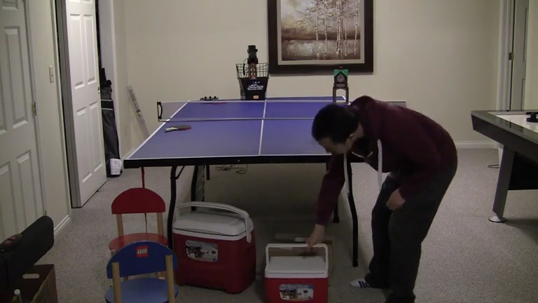
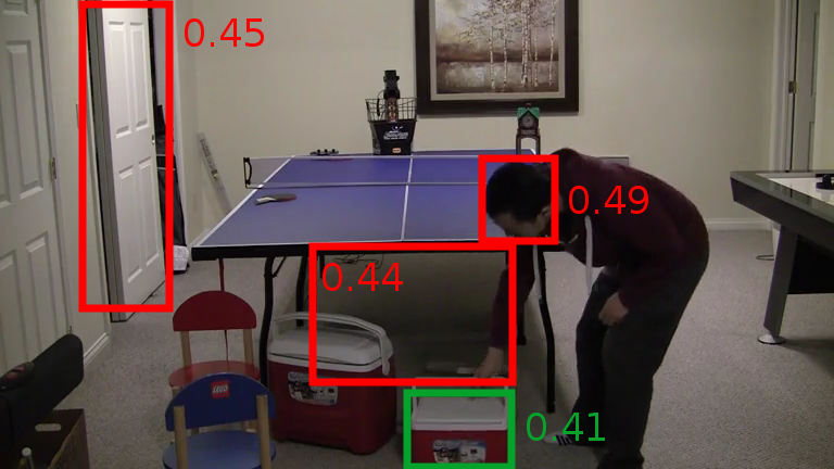
Figure 1: Object proposal confidence scores and saliency scores for a sample frame from our new dataset. Left: the original input video frame. Middle: several proposals and associated confidence scores produced by the method of Arbelaez et al. [4]. Note that the red boxes, which do not correspond to objects, let alone salient ones, all have higher scores than the green box, which does denote a salient object. Right: the saliency map output by the saliency detection method of Jiang et al. [21], currently the highest ranking method on the MIT saliency benchmark [10]. Note that the cooler is not highlighted as salient. Using these scores as part of the scoring function can drive the codetection process to produce undesired results.

The confidence score of a proposal can be a poor indicator of whether a proposal denotes a salient object, especially when objects are occluded, the lighting is poor, or motion blur exists (e.g., see Figure 1). Salient objects can have low confidence score while nonsalient objects or image regions that do not correspond to objects can have high confidence score. Thus our scoring function does not use the confidence scores produced by the proposal generation mechanism. Moreover, our method does not rely on human pose and depth information, which is not always available. Human pose can be difficult to estimate reliably when a person is only partially visible or is self-occluded [3], as is the case with most of our videos.

We avail ourselves of a different source of constraint on the codetection problem. In videos depicting human interaction with objects to be codetected, descriptions of such activity can impart weak spatial or motion constraint either on a single object or among multiple objects of interest. For example, if the video depicts a “pick up” event, some object should have an upward displacement during this process, which should be detectable even if it is small. This motion constraint will reliably differentiate the object which is being picked up from other stationary background objects. It is weak because it might not totally resolve the ambiguity; other image regions might satisfy this constraint, perhaps due to noise. Similarly, if we know object $A$ is on the left of object $B$, then the detection search for object $A$ will weakly affect the detection search for object $B$, and vice versa. To this end, we extract spatio-temporal constraints from sentences that describe the videos and then impose these constraints on the codetection process to find the most salient collections of objects that satisfy these constraints. Even though the constraints implied by a single sentence are usually weak, when accumulated across a set of videos and sentences, they together will greatly prune the detection search space. We call this process sentence directed video object codetection. It can be viewed as the inverse of video captioning/description [5, 14, 17] where object evidence (detections or other visual features) is first produced by pretrained detectors and then sentences are generated given the object appearance and movement.

Generally speaking, we extract a set of predicates from each sentence and formulate each predicate around a set of primitive functions. The predicates may be verbs (e.g., carried and rotated), spatial-relation prepositions (e.g., toTheLeftOf and above), motion prepositions (e.g., awayFrom and towards), or adverbs (e.g., quickly and slowly). The sentential predicates are applied to the candidate object proposals as arguments, allowing an overall predicate score to be computed that indicates how well these candidate object proposals satisfy the sentence semantics. We add this predicate score into the codetection framework, on top of the original similarity score, to guide the optimization. To the best of our knowledge, this is the first work that uses sentences to guide generic video object codetection. To summarize, our approach differs from the indicated prior work in the following ways:

1. Our method can codetect small or medium sized non-salient objects which can be located anywhere in the field of view.

2. Our method does not require or assume human pose or depth information.

3. Our method can codetect multiple objects simultaneously. These objects can be either moving in the foreground or stationary in the background.

4. Our method allows fast object movement and motion blur. Such is not exhibited in prior work.

5. Our method leverages sentence semantics to help codetection.

We evaluate our approach on two different datasets. The first is a new dataset that contains 15 distinct object classes and 150 video clips with a total of 12,509 frames. The second is a subset of CAD-120 [24], a dataset originally intended for activity recognition, that contains 5 distinct object classes and 75 video clips with a total of 8,854 frames. Our approach achieves an average IoU (Intersection-over-Union) score of 0.423 on the former and 0.373 on the latter. It yields an average detection accuracy of 0.7 to 0.8 on the former (when the IoU threshold is 0.4 to 0.3) and 0.5 to 0.6 on the latter (when the IoU threshold is 0.4 to 0.3).

2 Related Work

Corecognition is a simpler variant of codetection [44], where the objects of interest are sufficiently prominent in the field of view that the problem does not require object localization. Thus corecognition operates like unsupervised clustering, using feature extraction and the similarity measure. Codetection [7, 25, 42] additionally requires localization, often by putting bounding boxes around the objects. This can require combinatorial search over a large space of possible object locations. One way to remedy this is to limit the space of possible object locations to those produced by an object proposal method [1, 4, 46, 11]. These methods typically associate a confidence score with each proposal which can be used to prune or prioritize the search. Codetection is typically formulated as the process of selecting one proposal per image or frame, out of the many produced by the proposal mechanism, that maximizes the collective confidence of and similarity between the selected proposals. This optimization is usually performed with Belief Propagation [32] or with nonlinear programming. Recently, the codetection problem has been extended to video [40, 34, 22, 41, 35]. Like Srikantha and Gall [41], we codetect small and medium objects, but do so without using human pose or a depth map. Like Schulter et al. [40], we codetect both moving and stationary objects, but do so with a larger set of object classes and a larger video corpus. Also, like Ramanathan et al. [35], we use sentences to guide video codetection, but do so for a vocabulary that goes beyond pronouns, nominals, and names that are used to codetect only human face tracks.

Another line of work learns visual structures or models from image captions [30, 20, 19, 28, 6, 18], treating the input as a parallel image-text dataset. Since this work focuses on images and not video, the sentential captions only contain static concepts, such as the names of people or the spatial relations between objects in the images. In contrast, our approach models the motion and changing spatial relations that are present only in video as described by verbs and motion prepositions in the sentential annotation.

3 Sentence Directed Codetection

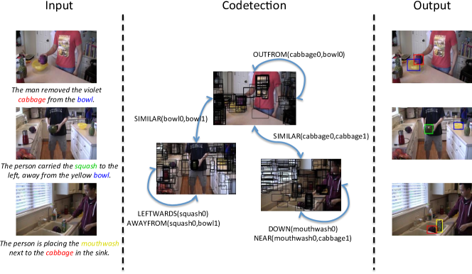
Figure 2: An overview of our codetection process. Left: input a set of videos paired with sentences. Middle: sentence directed codetection, where black bounding boxes represent object proposals. Right: output original videos with objects codetected. Note that no pretrained object detectors are used in this whole process. Also note how sentence semantics plays an important role in this process: it provides both unary scores, e.g., $\textsc{leftwards}(\textit{squash0})$ and $\textsc{down}(\textit{mouthwash0})$, for proposal confidence, and binary scores, e.g., $\textsc{outFrom}(\textit{cabbage0},\textit{bowl0})$ and $\textsc{near}(\textit{mouthwash0},\textit{cabbage1})$, for relating multiple objects in the same video. (Best viewed in color.)

Our sentence-directed codetection approach is illustrated in Figure 2. The input is a set of videos paired with human-elicited sentences, one sentence per video. A collection of object-candidate generators and video-tracking methods are applied to each video to obtain a pool of object proposals. Object instances and predicates are extracted from the paired sentence. Given multiple such video-sentence pairs, a graph is formed where object instances serve as vertices and similarities between object instances and predicates linking object instances in a sentence serve as edges. Finally, Belief Propagation is applied to this graph to jointly infer object codetections.

3.1 Sentence Semantics

Our main contribution is exploiting sentence semantics to help the codetection process. We use a conjunction of predicates to represent (a portion of) the semantics of a sentence. Object instances in a sentence fill the arguments of the predicates in that sentence. An object instance that fills the arguments of multiple predicates is said to be coreferenced. For a coreferenced object instance, only one track is codetected. For example, a sentence like “the person put the mouthwash into the sink near the cabbage” implies the following conjunction of predicates:

$$\textsc{down}(\textit{mouthwash})\wedge\textsc{near}(\textit{mouthwash},\textit{cabbage})$$

In this case, mouthwash is coreferenced by the predicates down (fills the sole argument) and near (fills the first argument). Thus only one mouthwash track will be produced, simultaneously constrained by the two predicates (Figure 2, blue track).

In principle, one could map sentences to conjunctions of our predicates using standard semantic parsing techniques [45, 12]. However, modern semantic parsers are domain specific, and employ machine-learning methods to train a semantic parser for a specific domain. No existing semantic parser has been trained on our domain. Training a new semantic parser requires a parallel corpus of sentences paired with intended semantic representations. Modern semantic parsers are trained with corpora like PropBank [31] that have tens of thousands of manually annotated sentences. Gathering such a large training corpus would be overkill for our experiments that involve only a few hundred sentences, especially since such is not our focus or contribution. Thus like Lin et al. [26], Kong et al. [23], and Plummer et al. [33], we employ simpler handwritten rules to fully automate the semantic parsing process for our limited corpus. Nothing, in principle, precludes using a machine-trained semantic parser in its place.

Our semantic parser employs seven steps.

1. Spelling errors are corrected with Ispell.

2. The NLTK parser is used to obtain the POS tags for each word in the sentence.

3. POS tagging errors are corrected by a postprocessing step with a small set of rules (Table Ia).

4. Words with a specified set of POS tags are eliminated.

5. NLTK is used to lemmatize all nouns and verbs.

6. Synonyms are conflated by mapping phrases to a smaller set of nouns and verbs using a small set of rules (Table Ib).

7. A small set of rules map the resulting word strings to predicates (Table Ic).

The entire process is fully automatic and implemented in less than two pages of Python code.

towards/IN ice chest/NN watering can/NN vegetable/NN watering pot/NN gas can/NN poured/VBD pineapple/NN box/NN blue/JJ violet/JJ pours/VBZ underneath/IN off/IN inside/IN place/VB	$\{\emph{gas can},\emph{gasoline can},\emph{gasoline tank}\}$ $\{\emph{put},\emph{set},\emph{place}\}$ $\{\emph{pick up},\emph{lift}\}$ $\{\emph{milk},\emph{almond milk},\emph{carton}\}$ $\{\emph{cooler},\emph{ice chest}\}$ $\{\emph{table},\emph{tennis table},\emph{ping pong table}\}$ $\{\emph{ground},\emph{driveway},\emph{floor}\}$ $\{\emph{bowl},\emph{dish},\emph{plate}\}$ $\{\emph{bucket},\emph{pail}\}$ $\{\emph{cabbage},\emph{vegetable}\}$ $\{\emph{box},\emph{cardboard box}\}$ $\{\emph{person},\emph{man},\emph{boy}\}$ $\{\emph{leftwards},\emph{leftward}\}$ $\{\emph{out},\emph{outside}\}$ $\{\emph{into},\emph{inside of},\emph{inside}\}$ $\{\emph{towards},\emph{toward}\}$ $\{\emph{on},\emph{onto}\}$	$\left.\begin{array}[]{l}\emph{person carry}\;x\;\emph{rightwards put it near}\;y\\ \emph{person carry}\;x\;\emph{leftwards put it near}\;y\\ \emph{person carry}\;x\;\emph{to right near}\;y\\ \emph{person carry}\;x\;\emph{to left near}\;y\\ \emph{person put}\;x\;\emph{on right near}\;y\\ \emph{person move}\;x\;\emph{from left to right near}\;y\\ \emph{person carry}\;x\;\emph{to left put it near}\;y\end{array}\right\}\leadsto\textsc{moveHorizontal}(x)\wedge\textsc{nearEnd}(x,y)$ $\left.\begin{array}[]{l}\emph{person move}\;x\;\emph{out of}\;y\\ \emph{person take}\;x\;\emph{out of}\;y\;\emph{put it to right}\\ \emph{person take}\;x\;\emph{out of}\;y\\ \emph{person take}\;x\;\emph{from}\;y\;\emph{put it on counter}\end{array}\right\}\leadsto\textsc{inStart}(x,y)\wedge\textsc{awayFrom}(x,y)$
up/RB down/RB blue/JJ drank/VBD pours/VBZ poured/VBD places/VBZ reaches/VBZ bowl/NN	$\{\emph{put},\emph{set},\emph{stack},\emph{place}\}$ $\{\emph{pick up},\emph{raise},\emph{lift}\}$ $\{\emph{drink},\emph{take drink},\emph{pick up drink}\}$ $\{\emph{take},\emph{remove}\}$ $\{\emph{cup},\emph{container},\emph{mug},\emph{tin}\}$ $\{\emph{cereal},\emph{cereal box},\emph{box}\}$ $\{\emph{water},\emph{liquid}\}$ $\{\emph{ground},\emph{floor}\}$ $\{\emph{on},\emph{onto}\}$	$\left.\begin{array}[]{l}\emph{person put}\;x\;\emph{into table}\\ \emph{person put}\;x\;\emph{on table}\\ \emph{person put down}\;x\\ \emph{person put}\;x\;\emph{down on table}\\ \emph{person put}\;x\;\emph{down}\end{array}\right\}\leadsto\textsc{moveDown}(x)$ $\left.\begin{array}[]{l}\emph{person pour}\;x\;\emph{into}\;y\\ \emph{person pick up}\;x\;\emph{pour it into}\;y\\ \emph{person pick up pour}\;x\;\emph{into}\;y\end{array}\right\}\leadsto\textsc{rotate}(x)\wedge\textsc{over}(x,y)$
(a)	(b)	(c)

TABLE I: Sample rules from (a) step 3, (b) step 6, and (c) step 7 of our semantic parser. (top) For our new dataset. (bottom) For the subset of CAD-120.

The rules employed by the last step of the above process generate a weak semantic representation, containing only those predicates that are relevant to our codetection process. For example, for the phrase “into the sink” in the above sentence, it is beyond our interest to detect the object sink. Thus our predefined rules generate $\textsc{down}(\textit{mouthwash})$ instead of $\textsc{into}(\textit{mouthwash},\textit{sink})$. Also, although a more detailed semantic representation for this sentence would include $\textsc{put}(\textit{person},\textit{mouthwash})$, we simplify this two-argument predicate to a one-argument predicate $\textsc{move}(\textit{mouthwash})$, since we do not attempt to codetect people. To ensure that we do not introduce surplus semantics, the generated predicates always implies a weaker constraint than the original sentence.

Each predicate is formulated around a set of primitive functions on the arguments of the predicate. The primitive functions produce scores indicating how well the arguments satisfy the constraint. The aggregate score over the functions constitutes the predicate score. Table II shows the complete list of our 24 predicates and the scores they compute. The function $\textsf{medFlMg}(p)$ computes the median of the average optical flow magnitude within the detections for the proposal $p$. The functions $\textsf{x}(p^{(t)})$ and $\textsf{y}(p^{(t)})$ return the $x$- and $y$-coordinates of the center of $p^{(t)}$, normalized by the frame width and height, respectively. The function distLessThan$(x,a)$ is defined as $\log[1/(1+\exp(-b(x-a)))]$, where we set $b=-20$ in the experiment. Similarly, the function $\textsf{distGreaterThan}(x,a)$ is defined as $\textsf{distLessThan}(-x,-a)$. The function $\textsf{dist}(p_{1}^{(t)},p_{2}^{(t)})$ computes the distance between the centers of $p_{1}^{(t)}$ and $p_{2}^{(t)}$, also normalized by the frame size. The function $\textsf{smaller}(p_{1}^{(t)},p_{2}^{(t)})$ returns 0 if the size of $p_{1}^{(t)}$ is smaller than that of $p_{2}^{(t)}$, and $-\infty$ otherwise. The function $\textsf{tempCoher}(p)$ evaluates whether the position of proposal $p$ changes during the video, by checking the position offsets between every two frames. A higher tempCoher score indicates that $p$ is more likely to be stationary in the video. The function $\textsf{rotAngle}(p^{(t)})$ computes the current rotated angle of the object inside $p^{(t)}$ by looking back 1 second (30 frames). We extract SIFT features [27] for both $p^{(t)}$ and $p^{(t-30)}$ and match them to estimate the similarity transformation matrix, from which the angle can be computed. Finally the function $\textsf{hasRotation}(\alpha,\beta)$ computes the rotation log-likelihood given angle $\alpha$ through the von Mises distribution for which we set the location $\mu=\beta$ and the concentration $\kappa=4$.

$\begin{array}[t]{c@{\hspace*{30pt}}c@{\hspace*{30pt}}c}\Delta\textsc{distLarge}\>{\scriptstyle\stackrel{{\scriptstyle\triangle}}{{=}}}\>0.25\hfil\hskip 30.&\Delta\textsc{distSmall}\>{\scriptstyle\stackrel{{\scriptstyle\triangle}}{{=}}}\>0.05\hfil\hskip 30.&\Delta\textsc{angle}\>{\scriptstyle\stackrel{{\scriptstyle\triangle}}{{=}}}\>\pi/2\end{array}$

$\begin{array}[t]{r@{\;\define\;}l}\textsc{move}(p)\;\>{\scriptstyle\stackrel{{\scriptstyle\triangle}}{{=}}}\>&\textsf{medFlMg}(p)\\ \textsc{moveUp}(p)\;\>{\scriptstyle\stackrel{{\scriptstyle\triangle}}{{=}}}\>&\textsc{move}(p)+\textsf{distLessThan}\left(\textsf{y}(p^{(T)})-\textsf{y}(p^{(1)}),-\Delta\textsc{distLarge}\right)\\ \textsc{moveDown}(p)\;\>{\scriptstyle\stackrel{{\scriptstyle\triangle}}{{=}}}\>&\textsc{move}(p)+\textsf{distGreaterThan}\left(\textsf{y}(p^{(T)})-\textsf{y}(p^{(1)}),\Delta\textsc{distLarge}\right)\\ \textsc{moveVertical}(p)\;\>{\scriptstyle\stackrel{{\scriptstyle\triangle}}{{=}}}\>&\textsc{move}(p)+\textsf{distGreaterThan}\left(\mathinner{\!\left\lvert\textsf{y}(p^{(T)})-\textsf{y}(p^{(1)})\right\rvert},\Delta\textsc{distLarge}\right)\\ \textsc{moveLeftwards}(p)\;\>{\scriptstyle\stackrel{{\scriptstyle\triangle}}{{=}}}\>&\textsc{move}(p)+\textsf{distLessThan}\left(\textsf{x}(p^{(T)})-\textsf{x}(p^{(1)}),-\Delta\textsc{distLarge}\right)\\ \textsc{moveRightwards}(p)\;\>{\scriptstyle\stackrel{{\scriptstyle\triangle}}{{=}}}\>&\textsc{move}(p)+\textsf{distGreaterThan}\left(\textsf{x}(p^{(T)})-\textsf{x}(p^{(1)}),\Delta\textsc{distLarge}\right)\\ \textsc{moveHorizontal}(p)\;\>{\scriptstyle\stackrel{{\scriptstyle\triangle}}{{=}}}\>&\textsc{move}(p)+\textsf{distGreaterThan}\left(\mathinner{\!\left\lvert\textsf{x}(p^{(T)})-\textsf{x}(p^{(1)})\right\rvert},\Delta\textsc{distLarge}\right)\\ \textsc{rotate}(p)\;\>{\scriptstyle\stackrel{{\scriptstyle\triangle}}{{=}}}\>&\textsc{move}(p)+\max\limits_{t}\textsf{hasRotation}\left(\textsf{rotAngle}(p^{(t)}),\Delta\textsc{angle}\right)\\ \textsc{towards}(p_{1},p_{2})\;\>{\scriptstyle\stackrel{{\scriptstyle\triangle}}{{=}}}\>&\textsc{move}(p_{1})+\textsf{distLessThan}\left(\textsf{dist}(p_{1}^{(T)},p_{2}^{(T)})-\textsf{dist}(p_{1}^{(1)},p_{2}^{(1)}),-\Delta\textsc{distLarge}\right)\\ \textsc{awayFrom}(p_{1},p_{2})\;\>{\scriptstyle\stackrel{{\scriptstyle\triangle}}{{=}}}\>&\textsc{move}(p_{1})+\textsf{distGreaterThan}\left(\textsf{dist}(p_{1}^{(T)},p_{2}^{(T)})-\textsf{dist}(p_{1}^{(1)},p_{2}^{(1)}),\Delta\textsc{distLarge}\right)\\ \textsc{leftOfStart}(p_{1},p_{2})\;\>{\scriptstyle\stackrel{{\scriptstyle\triangle}}{{=}}}\>&\textsf{tempCoher}(p_{2})+\textsf{distLessThan}\left(\textsf{x}(p_{1}^{(1)})-\textsf{x}(p_{2}^{(1)}),-\Delta\textsc{distSmall}\right)\\ \textsc{leftOfEnd}(p_{1},p_{2})\;\>{\scriptstyle\stackrel{{\scriptstyle\triangle}}{{=}}}\>&\textsf{tempCoher}(p_{2})+\textsf{distLessThan}\left(\textsf{x}(p_{1}^{(T)})-\textsf{x}(p_{2}^{(T)}),-\Delta\textsc{distSmall}\right)\\ \textsc{rightOfStart}(p_{1},p_{2})\;\>{\scriptstyle\stackrel{{\scriptstyle\triangle}}{{=}}}\>&\textsf{tempCoher}(p_{2})+\textsf{distGreaterThan}\left(\textsf{x}(p_{1}^{(1)})-\textsf{x}(p_{2}^{(1)}),\Delta\textsc{distSmall}\right)\\ \textsc{rightOfEnd}(p_{1},p_{2})\;\>{\scriptstyle\stackrel{{\scriptstyle\triangle}}{{=}}}\>&\textsf{tempCoher}(p_{2})+\textsf{distGreaterThan}\left(\textsf{x}(p_{1}^{(T)})-\textsf{x}(p_{2}^{(T)}),\Delta\textsc{distSmall}\right)\\ \textsc{onTopOfStart}(p_{1},p_{2})\;\>{\scriptstyle\stackrel{{\scriptstyle\triangle}}{{=}}}\>&\begin{array}[t]{@{}l@{}}\textsf{tempCoher}(p_{2})\\ +\textsf{distGreaterThan}\left(\textsf{y}(p_{1}^{(1)})-\textsf{y}(p_{2}^{(1)}),-2\Delta\textsc{distLarge}\right)\\ +\textsf{distLessThan}\left(\textsf{y}(p_{1}^{(1)})-\textsf{y}(p_{2}^{(1)}),0\right)\\ +\textsf{distLessThan}\left(\mathinner{\!\left\lvert\textsf{x}(p_{1}^{(1)})-\textsf{x}(p_{2}^{(1)})\right\rvert},2\Delta\textsc{distSmall}\right)\\ \end{array}\\ \textsc{onTopOfEnd}(p_{1},p_{2})\;\>{\scriptstyle\stackrel{{\scriptstyle\triangle}}{{=}}}\>&\begin{array}[t]{@{}l@{}}\textsf{tempCoher}(p_{2})\\ +\textsf{distGreaterThan}\left(\textsf{y}(p_{1}^{(T)})-\textsf{y}(p_{2}^{(T)}),-2\Delta\textsc{distLarge}\right)\\ +\textsf{distLessThan}\left(\textsf{y}(p_{1}^{(T)})-\textsf{y}(p_{2}^{(T)}),0\right)\\ +\textsf{distLessThan}\left(\mathinner{\!\left\lvert\textsf{x}(p_{1}^{(T)})-\textsf{x}(p_{2}^{(T)})\right\rvert},2\Delta\textsc{distSmall}\right)\\ \end{array}\\ \textsc{nearStart}(p_{1},p_{2})\;\>{\scriptstyle\stackrel{{\scriptstyle\triangle}}{{=}}}\>&\textsf{tempCoher}(p_{2})+\textsf{distLessThan}\left(\textsf{dist}(p_{1}^{(1)},p_{2}^{(1)}),2\Delta\textsc{distSmall}\right)\\ \textsc{nearEnd}(p_{1},p_{2})\;\>{\scriptstyle\stackrel{{\scriptstyle\triangle}}{{=}}}\>&\textsf{tempCoher}(p_{2})+\textsf{distLessThan}\left(\textsf{dist}(p_{1}^{(T)},p_{2}^{(T)}),2\Delta\textsc{distSmall}\right)\\ \textsc{inStart}(p_{1},p_{2})\;\>{\scriptstyle\stackrel{{\scriptstyle\triangle}}{{=}}}\>&\textsf{tempCoher}(p_{2})+\textsc{nearStart}(p_{1},p_{2})+\textsf{smaller}(p_{1}^{(1)},p_{2}^{(1)})\\ \textsc{inEnd}(p_{1},p_{2})\;\>{\scriptstyle\stackrel{{\scriptstyle\triangle}}{{=}}}\>&\textsf{tempCoher}(p_{2})+\textsc{nearEnd}(p_{1},p_{2})+\textsf{smaller}(p_{1}^{(T)},p_{2}^{(T)})\\ \textsc{belowStart}(p_{1},p_{2})\;\>{\scriptstyle\stackrel{{\scriptstyle\triangle}}{{=}}}\>&\textsf{tempCoher}(p_{2})+\textsf{distGreaterThan}\left(\textsf{y}(p_{1}^{(1)})-\textsf{y}(p_{2}^{(1)}),\Delta\textsc{distSmall}\right)\\ \textsc{belowEnd}(p_{1},p_{2})\;\>{\scriptstyle\stackrel{{\scriptstyle\triangle}}{{=}}}\>&\textsf{tempCoher}(p_{2})+\textsf{distGreaterThan}\left(\textsf{y}(p_{1}^{(T)})-\textsf{y}(p_{2}^{(T)}),\Delta\textsc{distSmall}\right)\\ \textsc{aboveStart}(p_{1},p_{2})\;\>{\scriptstyle\stackrel{{\scriptstyle\triangle}}{{=}}}\>&\textsf{tempCoher}(p_{2})+\textsf{distLessThan}\left(\textsf{y}(p_{1}^{(1)})-\textsf{y}(p_{2}^{(1)}),-\Delta\textsc{distSmall}\right)\\ \textsc{aboveEnd}(p_{1},p_{2})\;\>{\scriptstyle\stackrel{{\scriptstyle\triangle}}{{=}}}\>&\textsf{tempCoher}(p_{2})+\textsf{distLessThan}\left(\textsf{y}(p_{1}^{(T)})-\textsf{y}(p_{2}^{(T)}),-\Delta\textsc{distSmall}\right)\\ \textsc{over}(p_{1},p_{2})\;\>{\scriptstyle\stackrel{{\scriptstyle\triangle}}{{=}}}\>&\begin{array}[t]{@{}l@{}}\textsf{tempCoher}(p_{2})\\ +\max\limits_{t}\left(\begin{array}[]{@{}l@{}}\textsf{distLessThan}\left(\textsf{y}(p_{1}^{(t)})-\textsf{y}(p_{2}^{(t)}),-\Delta\textsc{distSmall}\right)\\ \textsf{distLessThan}\left(\mathinner{\!\left\lvert\textsf{x}(p_{1}^{(t)})-\textsf{x}(p_{2}^{(t)})\right\rvert},\Delta\textsc{distLarge}\right)\\ \end{array}\right)\\ \end{array}\\ \end{array}$

TABLE II: Our predicates and their semantics. For simplicity, we show the computation on only a single first frame $p^{(1)}$ or last frame $p^{(T)}$ of a proposal. In practice, to reduce noise, all of the scores are averaged over the first or last $L$ frames.

3.2 Generating Object Proposals

We first generate $N$ object candidates for each video frame. We use EdgeBoxes [46] to obtain the $\frac{N}{2}$ top-ranking object candidates and MCG [4] to obtain the other half, filtering out candidates larger than $\frac{1}{20}$ of the video-frame size to focus on small and medium-sized objects. This yields $NT$ object candidates for a video with $T$ frames. We then generate $K$ object proposals from these $NT$ candidates. To obtain object proposals with object candidates of consistent appearance and spatial location, one would nominally require that $K\ll N^{T}$. To circumvent this, we first randomly sample a frame $t$ from the video with probability proportional to the averaged magnitude of optical flow [15] within that frame. Then, we sample an object candidate from the $N$ candidates in frame $t$. To decide whether the object is moving or not, we sample from {moving,stationary} with distribution $\{\frac{1}{3},\frac{2}{3}\}$. We sample a moving object candidate with probability proportional to the average flow magnitude within the candidate. Similarly, we sample a stationary object candidate with probability inversely proportional to the average flow magnitude within the candidate. The sampled candidate is then propagated (tracked) bidirectionally to the start and the end of the video. We use the CamShift algorithm [9] to track both moving and stationary objects, allowing the size of moving objects to change during the process, but requiring the size of stationary objects to remain constant. Stationary objects are tracked to account for noise or occlusion that manifests as small motion or change in size. We track moving objects in HSV color space and stationary objects in RGB color space. We do not use optical-flow-based tracking methods since these methods suffer from drift when objects move quickly. We repeat this sampling and propagation process $K$ times to obtain $K$ object proposals $\{p_{k}\}$ for each video. Examples of the sampled proposals ($K=240$) are shown in the middle column of Figure 2.

3.3 Similarity between Object Proposals

We compute the appearance similarity of two object proposals as follows. We first uniformly sample $M$ detections $\{b^{m}\}$ from each proposal along its temporal extent. For each sampled detection, we extract PHOW [8] and HOG [13] features to represent its appearance and shape. We also do so after we rotate this detection by 90^∘, 180^∘, and 270^∘. Then, we measure the similarity $g$ between a pair of detections $b_{1}^{m}$ and $b_{2}^{m}$ with:

$$\begin{array}[]{r}g(b_{1}^{m},b_{2}^{m})=\max\limits_{i,j\in\{0,1,2,3\}}\frac{1}{2}\left(\begin{array}[]{l}g_{\chi^{2}}(\textrm{rot}_{i}(b_{1}^{m}),\textrm{rot}_{j}(b_{2}^{m}))\\ {}+g_{L_{2}}(\textrm{rot}_{i}(b_{1}^{m}),\textrm{rot}_{j}(b_{2}^{m}))\end{array}\right)\\ \end{array}$$

where $\textrm{rot}_{i}\;i=0,1,2,3$ represents rotation by 0^∘, 90^∘, 180^∘, and 270^∘, respectively. We use $g_{\chi^{2}}$ to compute the $\chi^{2}$ distance between the PHOW features and $g_{L_{2}}$ to compute the Euclidean distance between the HOG features, after which the distances are linearly scaled to $[0,1]$ and converted to log similarity scores. Finally, the similarity between two proposals $p_{1}$ and $p_{2}$ is taken to be:

$$g(p_{1},p_{2})=\mathop{\text{median}}\limits_{m}g(b_{1}^{m},b_{2}^{m})$$

	Our new dataset, codetection set #										Our subset of CAD-120, codetection set #
	1	2	3	4	5	6	7	8	9	10	1	2	3	4	5
Scene	k1	k2	k2,3	k4	b	b	g	k1,2,3	b&g	k1,2,3,4
Objects	box	bowl	bowl	cup	box	box	bucket	bowl	box	bowl	bowl	bowl	bowl	bowl	bowl
	cabbage	cabbage	cabbage	juice	cooler	cooler	gas can	cabbage	bucket	cabbage	cereal	cereal	cereal	cereal	cereal
	coffee grinder	coffee grinder	pineapple	ketchup			watering pot	pineapple	cooler	cup	cup	cup	cup	cup	cup
	mouthwash	mouthwash	squash	milk				squash	gas can	juice	jug	jug	jug	jug	jug
	pineapple	pineapple							watering pot	ketchup	microwave	microwave	microwave	microwave	microwave
	squash	squash								milk
										mouthwash
										pineapple
# of videos	26	27	17	21	19	17	23	17	25	24	15	15	15	15	15
# vertices in run 1	33	29	24	41	25	26	32	21	35	39	29	27	24	26	27
# vertices in run 2	34	37	32	46	24	22	27	26	32	41	25	27	24	22	27
# vertices in run 3	33	38	31	36	24	22	33	27	35	39	25	26	21	23	26

TABLE III: The experimental setup of the 10 codetection sets for our new dataset and the 5 codetection sets for our subset of CAD-120.

3.4 Joint Inference

We extract object instances (see all 15 classes for our new dataset and all 5 classes for our subset of CAD-120 in Section 4) from the sentences and model them as vertices in a graph. Each vertex $v$ can be assigned one of the $K$ proposals in the video that is paired with the sentence in which the vertex occurs. The score of assigning a proposal $k_{v}$ to a vertex $v$ is taken to be the unary predicate score $h_{v}(k_{v})$ computed from the sentence (if such exists, or otherwise 0). We construct an edge between every two vertices $v$ and $u$ that belong to the same object class. We denote this class membership relation as $(v,u)\in\mathcal{C}$. The score of this edge $(v,u)$, when the proposal $k_{v}$ is assigned to vertex $v$ and the proposal $k_{u}$ is assigned to vertex $u$, is taken to be the similarity score $g_{v,u}(k_{v},k_{u})$ between the two proposals, as described in Section 3.3. Similarly, we also construct an edge between two vertices $v$ and $u$ that are arguments of the same predicate. We denote this predicate membership relation as $(v,u)\in\mathcal{P}$. The score of this edge $(v,u)$, when the proposal $k_{v}$ is assigned to vertex $v$ and the proposal $k_{u}$ is assigned to vertex $u$, is taken to be the predicate score $h_{v,u}(k_{v},k_{u})$ between the two proposals, as described in Section 3.1. Our problem, then, is to select a proposal for each vertex that maximizes the joint score on this graph, i.e., solving the following optimization problem:

$$\max\limits_{\mathbf{k}}\sum_{v}h_{v}(k_{v})+\sum_{(v,u)\in\mathcal{C}}g_{v,u}(k_{v},k_{u})+\sum_{(v,u)\in\mathcal{P}}h_{v,u}(k_{v},k_{u})$$

where $\mathbf{k}$ is the collection of the selected proposals for all the vertices. Note that the unary and binary scores are equally weighted in the above objective function. This discrete inference problem on graphical models can be solved approximately by Belief Propagation [32]. In the experiment, we use the OpenGM [2] implementation to find the approximate solution.

4 Experiment

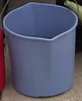
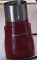
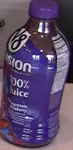
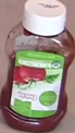
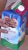
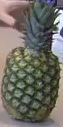
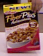
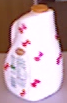
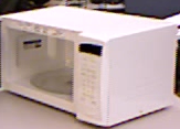
Figure 3: Examples of the 15 object classes to be codetected in our new dataset and the 5 object classes to be codetected in our subset of CAD-120. From left to right: the object classes in our new dataset, bowl, box, bucket, cabbage, coffee grinder, cooler, cup, gas can, juice, ketchup, milk, mouthwash, pineapple, squash, and watering pot, and the object classes in our subset of CAD-120, bowl, cereal, cup, jug, and microwave.

Our method can only be applied to datasets with the following properties:

1. It can only be applied to video that depicts motion and changing spatial relations between objects.

2. It can only be applied to video, not images, because it relies on such motion and changing spatial relations.

3. The video must be paired with sentences that describe that motion and those changing spatial relations. Some existing image and video corpora are paired with sentences that do not describe such.

4. The objects to be codetected must be detectable by existing object proposal methods.

5. There must be different clips that all involve different instances of the same object class participating in the described activity. This is necessary to support codetection.

Most existing datasets do not meet the above criteria and are thus ill suited to our approach. We evaluate on two specific datasets that are suited. Most existing methods require properties that our datasets lack. For example, Srikantha and Gall [41] require depth and human pose information. Others, such as Prest et al. [34], Schulter et al. [40], Joulin et al. [22], and Ramanathan et al. [35] do not make code available. Thus neither can one run our method on existing datasets or existing methods on our datasets.

It is not possible to compare our method to existing image codetection methods or evaluate on existing image codetection datasets, or any existing image captioning datasets, because they lack properties I, II, and III. Further, it is not possible to compare our method to existing video codetection methods or existing video codetection datasets. Schulter et al. [40] and Ramanathan et al. [35] address different problems with datasets that are highly specific to those problems and are thus incomparable. The dataset used by Prest et al. [34] and Joulin et al. [22] lacks properties I and III. Srikantha and Gall [41] evaluate on three datasets: ETHZ-activity [16], CAD-120, and MPII-cooking [38]. Two of the these, namely ETHZ-activity and MPII-cooking, lack properties III and IV. Srikantha and Gall [41] rely on depth and human pose information to overcome the lack of property IV. Moreover, the kinds of activity depicted in ETHZ-activity and MPII-cooking cannot easily be formulated in terms of descriptions of object motion and changing spatial relations. We do apply our method to a subset of CAD-120. However, because we do not use depth and human pose information, we only consider that subset of CAD-120 that satisfies property IV. Srikantha and Gall [41] apply their method to a different subject, rendering their results incomparable with ours. Moreover, we use incompatible sources of information: we use sentences but they do not; they use depth and human pose but we do not. This it is impossible to perform an apples-to-apples comparison, even on the common subset.

There exist a large number of video datasets that are not used for codetection but rather are used for others purposes like activity recognition and video captioning. Sentential annotation is available for some of these, like MPII-cooking, M-VAD [43], and MPII-MD [37]. However, the vast majority of the clips in M-VAD (48,986 clips annotated with sentences) and MPII-MD (68,337 clips annotated with sentences) do not satisfy properties I and IV. We searched the sentential annotations from each of these two corpora for all instances of twelve common English verbs that represent the kinds of verbs whose that describe motion and changing spatial relations between object.

	M-VAD		MPII-MD
add	89	0/10	120	0/10
carry	74	1/10	273	2/10
lift	435	1/10	374	0/10
load	48	0/10	89	0/10
move	332	0/10	1106	0/10
pick	366	1/10	703	1/10
pour	95	0/10	207	1/10
put	294	1/10	921	0/10
rotate	27	0/10	13	0/10
stack	91	0/10	56	0/10
take	1058	0/10	1786	0/10
unload	1	0/10	11	2/10

We further examined ten sentences for each verb from each corpus, together with the corresponding video clips, and found that only ten out of the 240 examined satisfied properties I and IV. Moreover, none of these ten suitable video clips satisfied property V. Further, of the twelve classes (AnswerPhone, DriveCar, Eat, FightPerson, GetOutCar, HandShake, HugPerson, Kiss, Run, SitDown, SitUp, and StandUp) in the Hollywood 2 dataset [29], only four (AnswerPhone, DriveCar, GetOutCar, and Eat) satisfy property I. Of these, three classes (AnswerPhone, DriveCar, and GetOutCar) always depict a single object class, and thus are ill suited for codetecting anything but the two fixed classes phone and car. The one remaining class (Eat) fails to satisfy property V. This same situation occurs with essentially all standard datasets used for activity recognition, like UCF Sports [36].

The standard sources of naturally occurring video for corpora used within the computer-vision community are Hollywood movies and YouTube video clips. However, Hollywood movies, in general, mostly involve dialog among actors, or generic scenery and backgrounds. At best, only small portions of most Hollywood movies satisfy property I, and such rarely is reflected in the dialog or script, thus failing to satisfy property III. We attempted to gather a codetection corpus from YouTube. But again, about a dozen students searching YouTube for depictions of about a dozen common English verbs, examining hundreds of hits, found that fewer than 1% satisfied property I and non satisfied property V. Thus it is only feasible to evaluate our method on video that has been filmed to expressly satisfy properties I–V.

While existing datasets within the computer-vision community do not satisfy properties I–V, we believe that these properties are nonetheless reflective of the real natural world. In the real world, people interact with everyday objects (in their kitchen, basement, driveway, and many similar location) all of the time. It is just that people don’t usually record such video, let alone make Hollywood movies about it or post it on YouTube. Further, people rarely describe such in naturally occurring text in movie scripts or in text uploaded to YouTube. Yet, children—and even adults—probably learn names of newly observed objects by observing people in their environment interacting with those objects in the context of dialog about such. Thus we believe that our problem, and our datasets, are a natural reflection of the kinds of learning that people employ to learn to recognize newly named objects.

4.1 Datasets

We evaluate our method on two datasets that do satisfy these properties. The first is a newly collected dataset, filmed to expressly satisfy properties I–V. This dataset was filmed in 6 different scenes (four in the kitchen, one in the basement, and one outside the garage) of a house. The lighting conditions vary greatly across the different scenes, with the basement scene the darkest, the kitchen scene exhibiting modest lighting, and the garage scene the brightest. Within each scene, the lighting often varies across different video regions. We assigned 5 actors (four adults and one child) with 15 distinct everyday objects (bowl, box, bucket, cabbage, coffee grinder, cooler, cup, gas can, juice, ketchup, milk, mouthwash, pineapple, squash, and watering pot, see Figure 3), and had them perform different actions which involve interaction with these objects. No special instructions were given requiring that the actors move slowly or the that objects not be occluded. The actors often are partially outside the field of view. Note that the dataset used by Srikantha and Gall [41] does not exhibit this property. Indeed, their method employs human pose which requires that the human be sufficiently visible to estimate such. The filming was performed using a normal consumer camera that introduces motion blur on the objects when the actors move quickly. We downsampled the filmed videos to $\text{768}\times\text{432}$ and divided them into 150 short video clips, each clip depicting a specific event lasting between 2 and 6 seconds at 30 fps. The 150 video clips constitute a total of 12,509 frames.

The second dataset is a subset of of CAD-120. Many of the 120 clips in CAD-120 depict sequences of actions. We divide those clips into subclips, each containing one action. We discard those that fail to satisfy any of the properties I, IV, or V, leaving 75 clips. These clips have spatial resolution $\text{640}\times\text{480}$, each clip depicting a specific event lasting between 3 and 5 seconds at 30 fps. The 75 video clips constitute a total of 8,854 frames, and contain 5 distinct object classes, namely bowl, cereal, cup, jug, and microwave.

4.2 Experimental Setup

We employed Amazon Mechanical Turk (AMT) to obtain three distinct sentences, by three different workers, for each video clip in each dataset, resulting in 450 sentences for the our new dataset and 225 sentences for our subset of CAD-120. AMT annotators were simply instructed to provide a single sentence for each video clip that described the primary activity depicted taking place with objects from a common list of object classes that occur in the entire dataset. The collected sentences were all converted to the predicates in Table II using the methods of Section 3.1. We processed each of the two datasets three times, each time using a different set of sentences produced by different workers; each sentence was used in exactly one run of the experiment. Furthermore, we divided each corpus into codetection set, each set containing a small subset of the video-sentence pairs. (For our new dataset, some pairs were reused in different codetection sets. For CAD-120, each pair was used in exactly one codetection set.) Some codetection sets contained only videos filmed in the same background, while others contained a mix of videos filmed in different backgrounds. (The backgrounds in each codetection set for our new dataset are summarized in Table III, where k, b, and g denote kitchen, basement, and garage, respectively.) This rules out the possibility of codetecting objects by simple background modeling (e.g., background subtraction). Codetection sets were processed independently, each with a distinct graphical model. Table III contains the number of video-sentence pairs and the number of vertices in the resulting graphical model for each codetection set of each corpus.

We compared the resulting codetections against human annotation. Human-annotated boxes around objects are provided with CAD-120. For our new dataset, these were obtained with AMT. We obtained five bounding-box annotations for each target object in each video frame. We asked annotators to annotate the referent of a specific highlighted word in the sentence associated with the video containing that frame. Thus the annotation reflects the semantic constraint implied by the sentences. This resulted in $\text{5}\times\text{289}=\text{1445}$ human annotated tracks. To measure how well codetections match human annotation, we use the IoU, namely the ratio of the area of the intersection of two bounding boxes to the area of their union. The object codetection problem exhibits inherent ambiguity: different annotators tend to annotate different parts of an object or make different decisions whether to include surrounding background regions when the object is partially occluded. To quantify such ambiguity, we computed intercoder agreement between the human annotators for our datasets. We computed $\frac{\text{5}\times{4}}{2}=\text{10}$ IoU scores for all box pairs produced by the 5 annotators in every frame and averaged them over the entire dataset, obtaining an overall human-human IoU of 0.72..

We found no publicly available implementations of existing video object codetection methods [34, 40, 22, 41, 35], thus for comparison we employ four variants of our method that alternatively disable different scores in our codetection framework. These variants help one understand the relative importance of different components of the framework. Together with our full method, they are summarized below:

	SIM	FLOW	SENT	SIM+FLOW	SIM+SENT
					(our full method)
Flow score?	no	yes	yes	yes	yes
Similarity score?	yes	no	no	yes	yes
Sentence score?	no	partial	yes	partial	yes

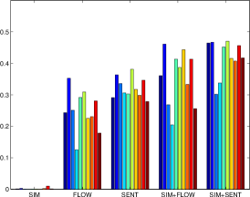
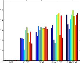
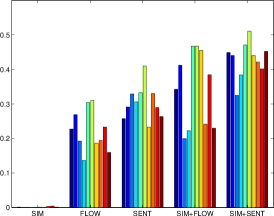
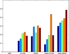
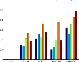
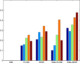
Run 1	Run 2	Run 3

Figure 4: IoU scores for different variants on different runs of different codetection sets on each dataset. (top) Our new dataset, codetection sets   1,   2,   3,   4,   5,   6,   7,   8,   9, and   10. (bottom) Our subset of CAD-120, codetection sets   1,   2,   3,   4, and   5.

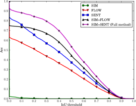
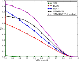
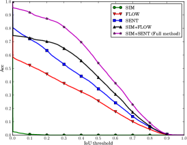
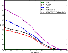
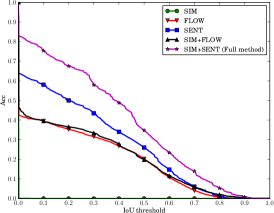
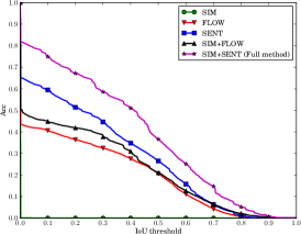
Run 1	Run 2	Run 3

Figure 5: The codetection accuracy curves of all five methods on our datasets. (top) Our new dataset. (bottom) Our subset of CAD-120.

Note that SIM uses the similarity measure but no sentential information. This method is similar to prior video codetection methods that employ similarity and the proposal confidence score output by proposal generation methods to perform codetection. When the proposal confidence score is not discriminative, as is the case with our datasets, the prior methods degrade to SIM. FLOW exploits only binary movement information from the sentence indicating which objects are probably moving and which are probably not (i.e., using only the functions medFlMg and tempCoher in Table II), without similarity or any other sentence semantics (thus “partial” in the table). SIM+FLOW adds the similarity score on top of FLOW. SENT uses all possible sentence semantics but no similarity measure. SIM+SENT is our full method that employs all scores. All the above variants were applied to each run of each codetection set of each dataset. Except for the changes indicated in the above table, all other parameters were kept constant across all such runs, thus resulting in an apples-to-apples comparison of the results. In particular, $N=500$, $K=240$, $M=20$, and $L=15$ (see Section 3 for details).

4.3 Results

We quantitatively evaluate our full method and all of the variants by computing $\text{IoU}_{\text{frame}}$, $\text{IoU}_{\text{object}}$, $\text{IoU}_{\text{set}}$, and $\text{IoU}_{\text{dataset}}$ for each dataset as follows. Given an output box for an object in a video frame, and the corresponding set of annotated bounding boxes (five boxes for our new dataset and a single box for CAD-120), we compute IoU scores between the output box and the annotated ones, and take the averaged IoU score as $\text{IoU}_{\text{frame}}$. Then $\text{IoU}_{\text{object}}$ is computed as the average of $\text{IoU}_{\text{frame}}$ over the output object track. Then, $\text{IoU}_{\text{set}}$ is computed as the average of $\text{IoU}_{\text{object}}$ over all the object instances in a codetection set. Then, $\text{IoU}_{\text{set}}$ is computed as the average of $\text{IoU}_{\text{object}}$ over all the object instances in a codetection set. Finally $\text{IoU}_{\text{dataset}}$ is computed as the average of $\text{IoU}_{\text{object}}$ over all runs of all codetection sets for a dataset.

We compute $\text{IoU}_{\text{set}}$ for each variant on each run of each codetection set in each dataset as shown in Figure 4. The first variant, SIM, using only the similarity measure, completely fails on this task as expected. However, combining SIM with either FLOW or SENT improves their performance. Moreover, SENT generally outperforms FLOW, both with and without the addition of SIM. Weak information obtained from the sentential annotation that indicates whether the object is moving or stationary, but no more, i.e., the distinction between FLOW and SENT, is helpful in reducing the object proposal search space, but without the similarity measure, the performance is still quite poor (FLOW). Thus one can get moderate results by combining just SIM and FLOW. But to further boost performance, more sentence semantics is needed, i.e., replacing FLOW with SENT. Further note that for our new dataset, SIM+FLOW ourperforms SENT, but for CAD-120, the reverse is true. This seems to be the case because CAD-120 has greater within-class variance so sentential information better supports codetection than image similarity. However, over-constrained semantics can, at times, hinder the codetection process rather than help, especially given the generality of our datasets. This is exhibited, for example, with codetection set 4 ( ) on run 1 of the CAD-120 dataset, where SIM+FLOW outperforms SIM+SENT. Thus it is important to only impose weak semantics on the codetection process.

Also note that there is little variation in $\text{IoU}_{\text{set}}$ across different runs within a dataset. Recall that the different runs were performed with different sentential annotations produced by different workers on AMT. This indicates that our approach is largely insensitive to the precise sentential annotation.

To evaluate the performance of our method in simply finding objects, we define codetection accuracy $\text{Acc}_{\text{frame}}$, $\text{Acc}_{\text{object}}$, $\text{Acc}_{\text{set}}$, and $\text{Acc}_{\text{dataset}}$ for each dataset as follows. Given an IoU threshold, we compute IoU scores between an output box and the corresponding annotated boxes, and binarize the scores according to a specified threshold. Then $\text{Acc}_{\text{frame}}$ is set to the maximum of the binarized scores, $\text{Acc}_{\text{object}}$ is computed as the average of $\text{Acc}_{\text{frame}}$ over the output object track, and $\text{Acc}_{\text{set}}$ is computed as the average of $\text{Acc}_{\text{object}}$ over all the object instances in a codetection set. Finally, we average $\text{Acc}_{\text{set}}$ scores over all runs of all codetection sets for a dataset to obtain $\text{Acc}_{\text{dataset}}$. By adjusting the IoU threshold from 0 to 1, we get an Acc-vs-threshold curve for each of the methods (Figure 5). It can be seen that the codetection accuracies of our full method under different IoU thresholds consistently outperform those of the variants. Our method yields an average detection accuracy (i.e., $\text{Acc}_{\text{dataset}}$) of 0.7 to 0.8 on the former (when the IoU threshold is 0.4 to 0.3) and 0.5 to 0.6 on the latter (when the IoU threshold is 0.4 to 0.3). Finally, we demonstrate some codetected object examples in Figure 6. For more examples, we refer the readers to our project page.

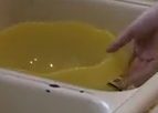
bowl

box

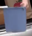
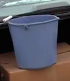
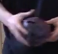
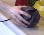
bucket

cabbage

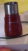
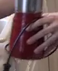
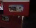
coffee grinder

cooler

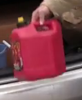
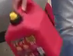
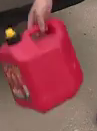
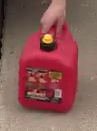
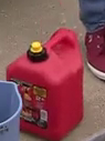
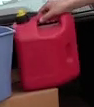
cup

gas can

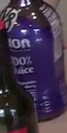
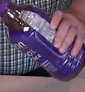
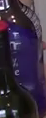
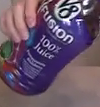
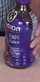
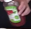
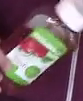
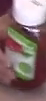
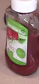
juice

ketchup

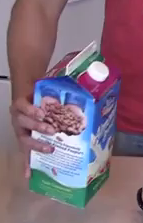
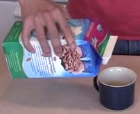
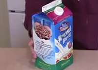
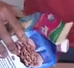
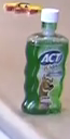
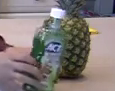
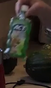
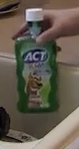
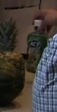
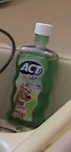
milk

mouthwash

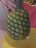
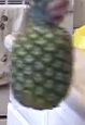
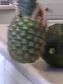
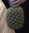
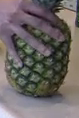
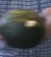
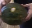
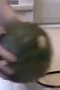
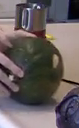
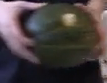
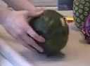
pineapple

squash

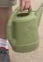
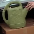
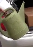
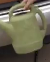
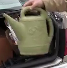
watering pot

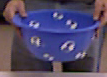
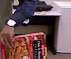
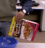
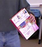
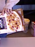
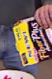
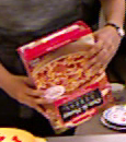
bowl

cereal

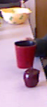
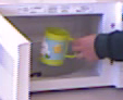
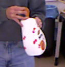
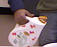
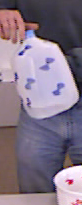
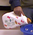
cup

jug

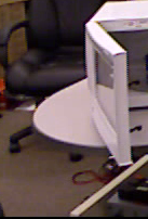
microwave

Figure 6: Examples of the 15 codetected object classes in our new dataset (top) and the 5 codetected object classes in our subset of CAD-120 (bottom). Note that in some examples the objects are occluded, rotated, poorly lit, or blurred due to motion, but they are still successfully codetected. (For demonstration purposes, the original output detections are slightly enlarged to include the surrounding context; zoom in on the screen for the best view).

5 Conclusion

We have developed a new framework for object codetection in video, namely, using natural language to guide codetection. Our experiments indicate that weak sentential information can significantly improve the results. This demonstrates that natural language, when combined with typical computer-vision problems, could provide the capability of high-level reasoning that yields better solutions to these problems.

Haonan Yu is currently a PhD student in the school of Electrical and Computer Engineering at Purdue University. He received the B.S. degree in Computer Science from Peking University, China, in 2011. His research interests are Computer Vision and Natural-Language Processing, especially combining video and language. He was the recipient of the Best Paper Award of ACL 2013.

Jeffrey Mark Siskind received the B.A. degree in computer science from the Technion, Israel Institute of Technology in 1979, the S.M. degree in computer science from MIT in 1989, and the Ph.D. degree in computer science from MIT in 1992. He did a postdoctoral fellowship at the University of Pennsylvania Institute for Research in Cognitive Science from 1992 to 1993. He was an assistant professor at the University of Toronto Department of Computer Science from 1993 to 1995, a senior lecturer at the Technion Department of Electrical Engineering in 1996, a visiting assistant professor at the University of Vermont Department of Computer Science and Electrical Engineering from 1996 to 1997, and a research scientist at NEC Research Institute, Inc. from 1997 to 2001. He joined the Purdue University School of Electrical and Computer Engineering in 2002 where he is currently an associate professor.

References

- Alexe et al. [2010] B. Alexe, T. Deselaers, and V. Ferrari. What is an object? In Proceedings of the IEEE Conference on Computer Vision and Pattern Recognition, pages 73–80, 2010.
- Andres et al. [2012] B. Andres, T. Beier, and J. H. Kappes. OpenGM: A C++ library for discrete graphical models. CoRR, abs/1206.0111, 2012.
- Andriluka et al. [2014] M. Andriluka, L. Pishchulin, P. Gehler, and B. Schiele. 2D human pose estimation: New benchmark and state of the art analysis. In Proceedings of the IEEE Conference on Computer Vision and Pattern Recognition, pages 3686–3693, 2014.
- Arbelaez et al. [2014] P. Arbelaez, J. Pont-Tuset, J. Barron, F. Marqués, and J. Malik. Multiscale combinatorial grouping. In Proceedings of the IEEE Conference on Computer Vision and Pattern Recognition, pages 328–335, 2014.
- Barbu et al. [2012] A. Barbu, A. Bridge, Z. Burchill, D. Coroian, S. Dickinson, S. Fidler, A. Michaux, S. Mussman, N. Siddharth, D. Salvi, L. Schmidt, J. Shangguan, J. M. Siskind, J. Waggoner, S. Wang, J. Wei, Y. Yin, and Z. Zhang. Video in sentences out. In Proceedings of the Conference on Uncertainty in Artificial Intelligence, pages 102–12, 2012.
- Berg et al. [2004] T. L. Berg, A. C. Berg, J. Edwards, M. Maire, R. White, Y. W. Teh, E. G. Learned-Miller, and D. A. Forsyth. Names and faces in the news. In Proceedings of the IEEE Conference on Computer Vision and Pattern Recognition, pages 848–854, 2004.
- Blaschko et al. [2010] M. Blaschko, A. Vedaldi, and A. Zisserman. Simultaneous object detection and ranking with weak supervision. In Advances in Neural Information Processing Systems, pages 235–243, 2010.
- Bosch et al. [2007] A. Bosch, A. Zisserman, and X. Munoz. Image classification using random forests and ferns. In Proceedings of the IEEE International Conference on Computer Vision, pages 1–8, 2007.
- Bradski [1998] G. R. Bradski. Computer vision face tracking for use in a perceptual user interface, 1998.
- Bylinskii et al. [2012] Z. Bylinskii, T. Judd, A. Borji, L. Itti, F. Durand, A. Oliva, and A. Torralba. MIT saliency benchmark, 2012.
- Cheng et al. [2014] M.-M. Cheng, Z. Zhang, W.-Y. Lin, and P. Torr. BING: Binarized normed gradients for objectness estimation at 300fps. In Proceedings of the IEEE Conference on Computer Vision and Pattern Recognition, pages 3286–3293, 2014.
- Clarke et al. [2010] J. Clarke, D. Goldwasser, M.-W. Chang, and D. Roth. Driving semantic parsing from the world’s response. In Proceedings of the Conference on Computational Natural Language Learning, pages 18–27, 2010.
- Dalal and Triggs [2005] N. Dalal and B. Triggs. Histograms of oriented gradients for human detection. In Proceedings of the IEEE Conference on Computer Vision and Pattern Recognition, pages 886–893, 2005.
- Das et al. [2013] P. Das, C. Xu, R. F. Doell, and J. J. Corso. A thousand frames in just a few words: Lingual description of videos through latent topics and sparse object stitching. In Proceedings of the IEEE Conference on Computer Vision and Pattern Recognition, pages 2634–2641, 2013.
- Farnebäck [2003] G. Farnebäck. Two-frame motion estimation based on polynomial expansion. In Proceedings of the Scandinavian Conference on Image Analysis, pages 363–370, 2003.
- Fossati et al. [2013] A. Fossati, J. Gall, H. Grabner, X. Ren, and K. Konolige. Consumer Depth Cameras for Computer Vision, chapter Human Body Analysis. Springer, 2013.
- Guadarrama et al. [2013] S. Guadarrama, N. Krishnamoorthy, G. Malkarnenkar, S. Venugopalan, R. Mooney, T. Darrell, and K. Saenko. YouTube2Text: Recognizing and describing arbitrary activities using semantic hierarchies and zero-shot recognition. In Proceedings of the IEEE International Conference on Computer Vision, pages 2712–2719, 2013.
- Gupta and Davis [2008] A. Gupta and L. S. Davis. Beyond nouns: Exploiting prepositions and comparative adjectives for learning visual classifiers. In Proceedings of the European Conference on Computer Vision, pages 16–29, 2008.
- Jamieson et al. [2010a] M. Jamieson, Y. Eskin, A. Fazly, S. Stevenson, and S. Dickinson. Discovering multipart appearance models from captioned images. In Proceedings of the European Conference on Computer Vision, pages 183–196, 2010a.
- Jamieson et al. [2010b] M. Jamieson, A. Fazly, S. Stevenson, S. J. Dickinson, and S. Wachsmuth. Using language to learn structured appearance models for image annotation. IEEE Transactions on Pattern Analysis and Machine Intelligence, 32(1):148–164, 2010b.
- Jiang et al. [2015] M. Jiang, S. Huang, J. Duan, and Q. Zhao. SALICON: Saliency in context. In Proceedings of the IEEE Conference on Computer Vision and Pattern Recognition, 2015.
- Joulin et al. [2014] A. Joulin, K. Tang, and L. Fei-Fei. Efficient image and video co-localization with Frank-Wolfe algorithm. In Proceedings of the European Conference on Computer Vision, pages 253–268, 2014.
- Kong et al. [2014] C. Kong, D. Lin, M. Bansal, R. Urtasun, and S. Fidler. What are you talking about? text-to-image coreference. In Proceedings of the IEEE Conference on Computer Vision and Pattern Recognition, pages 3558–3565, 2014.
- Koppula et al. [2013] H. S. Koppula, R. Gupta, and A. Saxena. Learning human activities and object affordances from RGB-D videos. International Journal of Robotics Research, 32(8):951–970, 2013.
- Lee and Grauman [2011] Y. J. Lee and K. Grauman. Learning the easy things first: Self-paced visual category discovery. In Proceedings of the IEEE Conference on Computer Vision and Pattern Recognition, pages 1721–1728, 2011.
- Lin et al. [2014] D. Lin, S. Fidler, C. Kong, and R. Urtasun. Visual semantic search: Retrieving videos via complex textual queries. In Proceedings of the IEEE Conference on Computer Vision and Pattern Recognition, pages 2657–2664, 2014.
- Lowe [2004] D. G. Lowe. Distinctive image features from scale-invariant keypoints. International Journal of Computer Vision, 60(2):91–110, 2004.
- Luo et al. [2009] J. Luo, B. Caputo, and V. Ferrari. Who’s doing what: Joint modeling of names and verbs for simultaneous face and pose annotation. In Advances in Neural Information Processing Systems, pages 1168–1176, 2009.
- Marszałek et al. [2009] M. Marszałek, I. Laptev, and C. Schmid. Actions in context. In Proceedings of the IEEE Conference on Computer Vision and Pattern Recognition, pages 2929–2936, 2009.
- Moringen et al. [2008] J. Moringen, S. Wachsmuth, S. Dickinson, and S. Stevenson. Learning visual compound models from parallel image-text datasets. Pattern Recognition, 5096:486–496, 2008.
- Palmer et al. [2005] M. Palmer, D. Gildea, and P. Kingsbury. The proposition bank: An annotated corpus of semantic roles. Computational linguistics, 31(1):71–106, 2005.
- Pearl [1982] J. Pearl. Reverend Bayes on inference engines: a distributed hierarchical approach. In Proceedings of the Conference on Artificial Intelligence, pages 133–136, 1982.
- Plummer et al. [2015] B. Plummer, L. Wang, C. Cervantes, J. Caicedo, J. Hockenmaier, and S. Lazebnik. Flickr30k entities: Collecting region-to-phrase correspondences for richer image-to-sentence models. In Proceedings of the IEEE International Conference on Computer Vision, 2015.
- Prest et al. [2012] A. Prest, C. Leistner, J. Civera, C. Schmid, and V. Ferrari. Learning object class detectors from weakly annotated video. In Proceedings of the IEEE Conference on Computer Vision and Pattern Recognition, pages 3282–3289, 2012.
- Ramanathan et al. [2014] V. Ramanathan, A. Joulin, P. Liang, and L. Fei-Fei. Linking people with “their” names using coreference resolution. In Proceedings of the European Conference on Computer Vision, pages 95–110, 2014.
- Rodriguez et al. [2008] M. D. Rodriguez, J. Ahmed, and M. Shah. Action MACH: A spatio-temporal maximum average correlation height filter for action recognition. In Proceedings of the IEEE Conference on Computer Vision and Pattern Recognition, pages 1–8, 2008.
- Rohrbach et al. [2015] A. Rohrbach, M. Rohrbach, N. Tandon, and B. Schiele. A dataset for movie description. In Proceedings of the IEEE Conference on Computer Vision and Pattern Recognition, 2015.
- Rohrbach et al. [2012] M. Rohrbach, S. Amin, M. Andriluka, and B. Schiele. A database for fine grained activity detection of cooking activities. In Proceedings of the IEEE Conference on Computer Vision and Pattern Recognition, pages 1194–1201, 2012.
- Rubinstein et al. [2013] M. Rubinstein, A. Joulin, J. Kopf, and C. Liu. Unsupervised joint object discovery and segmentation in internet images. In Proceedings of the IEEE Conference on Computer Vision and Pattern Recognition, pages 1939–1946, 2013.
- Schulter et al. [2013] S. Schulter, C. Leistner, P. M. Roth, and H. Bischof. Unsupervised object discovery and segmentation in videos. In Proceedings of the British Machine Vision Conference, pages 53.1–53.12, 2013.
- Srikantha and Gall [2014] A. Srikantha and J. Gall. Discovering object classes from activities. In Proceedings of the European Conference on Computer Vision, pages 415–430, 2014.
- Tang et al. [2014] K. Tang, A. Joulin, J. Li, and L. Fei-Fei. Co-localization in real-world images. In Proceedings of the IEEE Conference on Computer Vision and Pattern Recognition, pages 1464–1471, 2014.
- Torabi et al. [2015] A. Torabi, P. Chris, L. Hugo, and C. Aaron. Using descriptive video services to create a large data source for video annotation research. CoRR, abs/1503.01070, 2015.
- Tuytelaars et al. [2010] T. Tuytelaars, C. H. Lampert, M. B. Blaschko, and W. L. Buntine. Unsupervised object discovery: A comparison. International Journal of Computer Vision, 88(2):284–302, 2010.
- Wong and Mooney [2007] Y. W. Wong and R. J. Mooney. Learning synchronous grammars for semantic parsing with lambda calculus. In Proceedings of the Annual Meeting of the Association for Computational Linguistics, pages 960–967, 2007.
- Zitnick and Dollár [2014] C. L. Zitnick and P. Dollár. Edge boxes: Locating object proposals from edges. In Proceedings of the European Conference on Computer Vision, pages 391–405, 2014.