Moments of the inverse participation ratio for the Laplacian on finite regular graphs

Abstract

We investigate the first and second moments of the inverse participation ratio (IPR) for all eigenvectors of the Laplacian on finite random regular graphs with $n$ vertices and degree $z$. By exactly diagonalizing a large set of $z$-regular graphs, we find that as $n$ becomes large, the mean of the inverse participation ratio on each graph, when averaged over a large ensemble of graphs, approaches the numerical value $3$. This universal number is understood as the large-$n$ limit of the average of the quartic polynomial corresponding to the IPR over an appropriate $(n-2)$-dimensional hypersphere of $\mathbb{R}^{n}$. For a large, but not exhaustive ensemble of graphs, the mean variance of the inverse participation ratio for all graph Laplacian eigenvectors deviates from its continuous hypersphere average due to large graph-to-graph fluctuations that arise from the existence of highly localized modes.

1 Introduction

Much of condensed matter physics involves the study of either localized or itinerant degrees of freedom that exist on the sites of a Euclidean lattice, defined by a notion of physical distance between a site and some number of proximate or “neighboring” ones. The relationship between a site and its neighbors defines both the dimension of space, $d$ and a finite set of lattice vectors $a_{j}\in\mathbb{R}^{d}$, $j=1,\ldots,d$ that can be used in combination with a set of integers $\{\boldsymbol{m}\}$ with $\boldsymbol{m}_{i}\in\mathbb{Z}^{d}$ to index $n$ lattice sites via $\boldsymbol{R}_{i}=\sum_{j=1}^{d}m_{ij}a_{j}$. Examples include the fourteen Bravais lattices in three spatial dimensions. However, it is often instructive to consider the same physical degrees of freedom on a non-Euclidean lattice, or graph, where no distance metric exists. A finite lattice of $n$ sites is replaced by a graph $G$, consisting of a set of vertices $V=\{v_{i}\}$, each connected by $z_{i}$ undirected edges to its neighboring vertices. The quantity $z_{i}$ is known as the degree of the vertex $v_{i}$, and is equivalent to twice the spatial dimension for a hypercubic lattice.

Studying a given physical model on a graph offers many technical benefits including the ability to: (i) study arbitrarily long range interactions where exact mean-field solutions may be available, (ii) smoothly tune and control the local dimensionality and (iii) easily encode the randomness and disorder that often exists in real systems. Celebrated examples from statistical physics include the solution of the Ising model and its generalizations; graph coloring and random percolation problems (for a review see Ref. [1]). Anderson’s model of non-interacting electrons hopping on a disordered lattice [2] was first solved on the Cayley tree (Bethe lattice) [3], providing deep physical insights into the nature of localization in quantum mechanical systems. More recently, the ability to study graphs in the limit $z\to\infty$ has lead to the development of Dynamical Mean Field Theory [4], allowing for systematic investigations of candidate microscopic models of the high temperature superconductors [5].

The discrete Laplacian matrix $L$ plays a crucial role in defining any physical model on a graph, as it quantifies the energy cost of rapidly varying some local degree of freedom among a set of neighboring vertices. For example, it encodes the classical dynamics in random vibrational networks [6] as well the onset of ferromagnetism in the classical [7] and quantum $\mathrm{O}(n)$ model [8, 9] on graphs. It appears in models of non-interacting bosons hopping between graph vertices, where the existence of a Bose-Einstein condensation transition on complex networks can be rigorously proven [10].

In this paper, we are interested in the properties of the Laplacian defined on finite sized regular graphs, defined by the constraint that each of the $n$ vertices is connected to exactly $z$ neighbors. Examples with $n=100$ and $z=3,8$ are shown in Fig. 1.

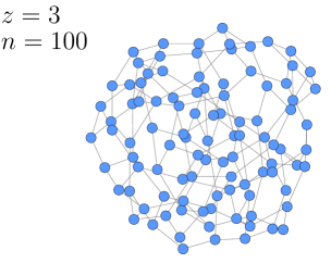
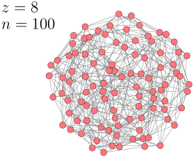
Figure 1: Regular graphs with $n=100$ vertices and degrees $z=3$ and $z=8$ constructed using NetworkX [11] via the Steger-Wormald algorithm [12, 13].

Such graphs possess many important mathematical properties [14] while still retaining similarities to the physically realizable Bravais lattices discussed above.

Much is known about the spectral properties of random regular graphs, both in the thermodynamic limit $n\to\infty$ [15, 16, 17] and more recently, at finite (but large) $n$ [18, 19, 20, 21]. The analyses of spectral statistics have yielded fruitful and universal connections [22] between random regular graphs and the Gaussian Orthogonal Ensemble of random matrix theory [23, 24, 25] known to be relevant in describing the fluctuations of energy levels in physical dynamical systems.

Substantially less is known about the eigenvectors of $L$ [26] with early work focusing on empirical analyses of nodal domains [27, 28] or specific vectors [29], as as it is not possible to apply many of the standard tools of analysis for Euclidean lattices, including the Fourier transform. Subsequently, a series of results [18, 30, 31, 21] have shown that for suitably large $n$, the eigenvectors of random regular graphs are delocalized – they have few non-zero entries. Very recently, the breakthrough works of Bourgade, Huang, and Yau [32] and Backhausz and Szegedy [33] have proven exiting new results that the eigenvector components are Gaussian independent and identically distributed for large $n$. To our knowledge, the physical implications of these new results for finite realizations of $z$ and $n$ amenable to direct numerical analysis have yet to be explored.

To address this gap, we systematically study the eigenvectors of the Laplacian matrix on a large class of finite size random regular graphs through brute-force numerical diagonalization. We investigate the statistics of the inverse participation ratio, a scalar proxy for localization, and numerically observe that its mean across all eigenvectors approaches a finite universal value equal to $3$, independent of graph degree. We quantify the second moment of the distribution and find a dependence both on degree $z$ and the number of vertices $n$.

The paper is organized as follows: we begin with a formal definition of the discrete Laplacian on graphs in Section 2 and describe our numerical results for the inverse participation ratio in Section 3. In Section 4, we analyze the inverse participation ratio as a polynomial function on an $(n-2)$-dimensional subsphere of $n$-dimensional real space. This perspective allows us to calculate exact values for the first and second moments of the inverse participation ratio over a continuous domain which contains the (terminal points of the) eigenvectors of the Laplacian. Section 5 compares the values of the theoretically derived moments to those numerically computed from a large set of finite size random regular graphs. We analyze the deviations from the theoretically derived second moment with a discussion of localized eigenvectors and highlight implications for their use in computing physical observables on finite random regular graphs.

2 The Graph Laplacian

The Laplacian matrix generalizes the continuous Laplace operator $\Delta\equiv\boldsymbol{\nabla}\cdot\boldsymbol{\nabla}$ to encode variations of any continuous function $\phi:V\to\mathbb{C}$ which can take a value $\phi_{i}$ on the vertex $v_{i}$. The physical importance of this matrix stems from the fact that solutions of $\Delta\phi=0$ correspond to the Dirichlet energy functional which is stationary in some spatial region. The particular extension of $\Delta$ to a graph that we employ arises from the discrete approximation to the second continuous derivative of $\phi$ on a hypercubic lattice in $d$ spatial dimensions with unit lattice spacing:

$$\Delta\phi(\boldsymbol{R}_{i})\approx\sum_{j=1}^{d}\left[\phi\left(\boldsymbol{R}_{i}+\boldsymbol{e}_{j}\right)+\phi\left(\boldsymbol{R}_{i}-\boldsymbol{e}_{j}\right)-2\phi\left(\boldsymbol{R}_{i}\right)\right]$$ (1)

where $\boldsymbol{e}_{j}$ are the Cartesian unit vectors with elements $e_{kj}=\delta_{kj}$ and $\delta_{kj}$ is the Kronecker $\delta$-function. On a regular graph $G$ consisting of $n$ vertices $v_{i}$, each with degree $z$, the local connectivity is encoded in an adjacency matrix $A_{ij}$ where

$$A_{ij}=\left\{\begin{array}[]{rcl}1&;&\mbox{if }v_{i}\mbox{ and }v_{j}\mbox{ share an edge},\\ 0&;&\mbox{otherwise}.\end{array}\right.\,$$ (2)

Comparing with Eq. (1), we can write the elements of the graph Laplacian matrix as the difference between the degree and adjacency matrices of $G$:

$$L_{ij}=z\delta_{ij}-A_{ij}$$ (3)

and observe that $z$ corresponds to twice the dimension on a hypercubic lattice. As mentioned in the introduction, $L$ may appear in the Hamiltonian of numerous physical systems defined on a graph in the form:

$$H=\frac{1}{2}\sum_{i,j=1}^{n}\phi^{\ast}_{i}L_{ij}\phi^{\phantom{\ast}}_{j}.$$ (4)

A spectral decomposition of $L$ provides a route to the determination of the equations of motion governing a classical system, or the nature of the wavefunctions and allowed energy eigenstates for a quantum mechanical one.

2.1 Exact diagonalization

We now focus on the spectral decomposition of Laplacian matrices drawn from an ensemble of random regular graphs with with $n$ vertices and degree $z$. These matrices are generated using the $\mathrm{O}(nz^{2})$ algorithm of Steger and Wormald [12]. From the vertex neighbor list of each graph, we construct the adjacency matrix $A$ and then exactly diagonalize the resulting $n\times n$ sparse Laplacian matrix $L$ given in Eq. (3). In this paper, we present results for graphs with

$$z \in\{3,4,5,10,15,20,25,30,35,40,45,50\}$$

$$n \in\{200,300,400,500,1000,2000,3000,4000,5000,10000\}$$

where $z$ and $n$ have been chosen with an eye towards exploring their interdependence for large graphs. All averages are performed over a set containing $N_{G}$ graph realizations, with $N_{G}=5000$ for $n<5000$ and $N_{G}=1000$ graphs for $n\geq 5000$. The exact number of unique graphs, $\mathcal{N}_{G}$ with a given $n$ and $z$ grows quickly with $n$ but is unknown in general. An asymptotic result for degrees satisfying $z\leq\sqrt{2\log n}-1$ was proved by Bollobás in Ref. [34]. Explicit counts for small $n$ and $z$ can be found at the Online Encyclopedia of Integer Sequences [35], e.g. for $z=3$ and $n=16$, $\mathcal{N}_{G}=4060$.

We begin our analysis by describing the eigenvalue distribution of $L$. For $n\gg 1$, the limiting form of the density of states $\rho(\varepsilon)$, the probability of an eigenvalue falling between $\varepsilon$ and $\varepsilon+d\varepsilon$, is given by the Kesten-McKay law [15, 16, 20]:

$$\rho(\varepsilon)=\frac{1}{n}\delta(\varepsilon)+\frac{z}{2\pi}\frac{\sqrt{4(z-1)-(\varepsilon-z)^{2}}}{z^{2}-(\varepsilon-z)^{2}}\quad;\quad|\varepsilon-z|\leq 2\sqrt{z-1}.$$ (5)

For finite values of $n$, Metz et al. have recently computed the $1/n$ corrections to this expression, originating from the contributions of loops of all possible lengths.

For a graph with $n$ vertices, the eigenvalues of the Laplacian matrix $\{\varepsilon_{i}\}$ are determined by exact diagonalization, and a comparison to Eq. (5) can be made by numerically constructing the histogram:

$$\expectationvalue{\rho(\varepsilon)}=\expectationvalue{\frac{1}{n}\sum_{i=1}^{n}\delta(\varepsilon-\varepsilon_{i})}$$ (6)

where an average over $N_{G}$ graph realizations is indicated by the angle brackets: $\langle\cdots\rangle\equiv(1/N_{G})\sum_{G}(\cdots)$. The results for $n=1000$, $z=3,4,5,10,20,50$ and $N_{G}=5000$ are shown in Fig. 2.

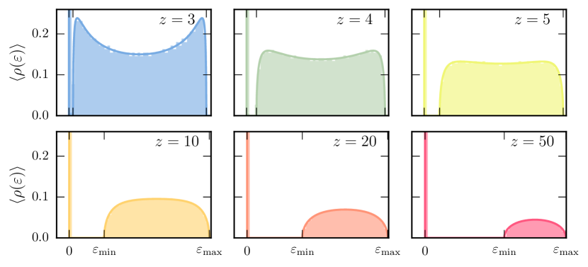
Figure 2: The probability of graph Laplacian eigenvalues for $n=1000$ vertices with degrees $z=3,4,5,10,20,50$ computed by diagonalizing numerically constructed graphs (shaded region) compared with the large-$n$ limit Kesten-McKay law defined in Eq. (5) (solid line). Eigenvalues in the continuum are bounded between $\varepsilon_{\mathrm{min}}=z-2\sqrt{z-1}$ and $\varepsilon_{\mathrm{max}}=z+2\sqrt{z-1}$, while the Perron-Frobenius mode with weight $1/n$ is shown as a spike at $\varepsilon=0$.

We observe only small graph-to-graph variations and find excellent agreement with the Kesten-McKay semi-circle law of Eq. (5) using $50$ eigenvalue bins (solid line). For $n>1000$ there is no visible discrepancy on this scale between the numerical results and the prediction for the large $n$ limit. For finite sized random regular graphs, the spectrum of the Laplacian consists of a single eigenvalue at $\varepsilon=0$ separated by a $z$-dependent gap [36] to a quasi-continuum of eigenvalues bounded between $\varepsilon_{\mathrm{min}}=z-2\sqrt{z-1}$ and $\varepsilon_{\mathrm{max}}=z+2\sqrt{z-1}$.

3 The Inverse Participation Ratio

Less is understood about the set of eigenvectors $E=\{\boldsymbol{x}\,:\,L\boldsymbol{x}=\varepsilon\boldsymbol{x}\}$ [27, 28, 17] although for certain classes of regular graphs with $z\sim\mathrm{O}(n)$, they are believed (with high probability [18]) to be delocalized – meaning they have many non-zero components. The eigenvalue $\varepsilon=0$ with weight $1/n$ in Eq. (5) and Fig. 3 corresponds to the special case of the Perron-Frobenius mode: $\wp\equiv(1/\sqrt{n},\ldots,1/\sqrt{n})$ and via orthogonality it follows that $\boldsymbol{x}\cdot\wp=\sum_{i}x_{i}=0$ for any eigenvector $\boldsymbol{x}\neq\wp$. We wish to develop an understanding of the properties of the remaining eigenvectors $\mathcal{E}\equiv E\setminus\{\wp\}$, and in particular, determine how the non-zero elements of an arbitrary $\boldsymbol{x}\in\mathcal{E}$ are distributed amongst its $n$ coordinates.

To this end, we study the notion of localization of an eigenvector using the inverse participation ratio. Historically, the participation ratio $p$ was introduced to aid in classifying the properties of atomic vibrations in disordered lattices [37]. It describes the fraction of the total number of sites which participate in a given normal mode vibration corresponding to the eigenvector $\boldsymbol{x}=(x_{1},\ldots,x_{n})\in\mathbb{R}^{n}$ and takes the value

$$p(\boldsymbol{x})=\frac{(\mu^{1})^{2}}{\mu^{0}\mu^{2}}$$ (7)

where $\mu^{r}=\sum_{i=1}^{n}|x_{i}|^{2r}$ can be thought of as the $r^{\mathrm{th}}$ moment of the kinetic energy of the mode. If a given normal mode only involves the motion of a single atom, it is characterized as localized and has $p=1/n$. A vibrational mode consisting of all atoms participating equally is called extended and has $p=1$. An equivalent measure was employed by Visscher [38] to study the degree of localization of electronic eigenstates in the Anderson model [2] with implications for the existence of a metal-insulator (delocalization-localization) transition in the presence of disorder.

When considering normalized eigenvectors $\boldsymbol{x}\cdot\boldsymbol{x}=||\boldsymbol{x}||=1$, it is often more convenient to consider the associated inverse participation ratio (IPR):

$$\frac{1}{p(\boldsymbol{x})}\equiv{IPR}(\boldsymbol{x})=n\sum_{i=1}^{n}x_{i}^{4}.$$ (8)

For the Laplacian matrix in Eq. (3) with $\boldsymbol{x}\in E$ we have

$$1\leq{IPR}(\boldsymbol{x})\leq\frac{n}{2}$$ (9)

with bounds corresponding to the extended Perron-Frobenius (lower bound) and localized (upper bound) modes, respectively. The finite size scaling of ${IPR}(\boldsymbol{x})/n$ as $n\to\infty$ provides information on the existence of a mobility edge, which defines the portion of the spectrum with robust delocalized states. This scaling has been extensively studied for a large class of random matrices [39, 40, 41, 42].

The inverse participation ratio thus provides a convenient single scalar value measuring the degree to which a particular eigenvector is localized ($p^{-1}\sim\mathrm{O}(n)$) or extended ($p^{-1}\sim\mathrm{O}(1)$). To obtain information on the reduced set of Laplacian eigenvectors $\mathcal{E}$ corresponding to non-zero eigenvalues, we construct a histogram of values in analogy with Eq. (6). The non-linear form of the IPR necessitates that the order of averaging is important, and we must compute

$$\rho(\mathrm{IPR})=\frac{1}{n-1}\sum_{\boldsymbol{x}\in\mathcal{E}}\delta(\mathrm{IPR}-{IPR}(\boldsymbol{x}))$$ (10)

for each graph realization separately before averaging over graphs. The resulting graph averaged distributions are shown in Fig. 3 for $n=1000$, $z=3,4,5,10,20,50$ and $N_{G}=5000$.

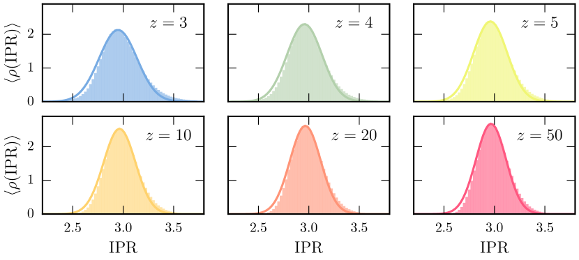
Figure 3: Histograms of IPR values for the Laplacian matrix on random regular graphs with $n=1000$ vertices and degrees $z={3,4,5,10,20,50}$. Solid lines represent fits to a Gaussian distribution.

The solid lines show the results of a fit to a Gaussian distribution for each $n$ and $z$ and there are clear deviations which skew to larger IPR values, most notably for small $z$. For fixed $n$, increasing $z$ decreases the width of the distribution, and slightly improves the residual of the Gaussian fit, but quite strikingly, the mean stays at a value that is numerically very close to $3$, with the result appearing to be exact as $n\to\infty$.

This empirical finding warrants an explanation, which we provide subsequently in Section 4. In order to motivate our approach, we appeal to progress in understanding the statistics of eigenvectors in the more general setting of random matrix theory. Recently, Bourgade, Huange, and Yau in [32] and Backhausz and Szegedy [33] undertook a systematic study of eigenvector statistics of sparse random matrices. They recovered specific information about the eigenvectors of adjacency matrices of random regular graphs whose degree $z$ is bounded by the number of vertices $n$. Mirroring the hypothesis in Ref. [32], let $\delta>0$ be an arbitrarily small constant. For a random $z$-regular graph which satisfies $n^{\delta}\leq z\leq n^{2/3-\delta}$ their main result, Theorem 1.1, implies that the entries of those eigenvectors of random regular graphs which are orthogonal to the Perron-Frobenius mode $\wp$ have asymptotically independent Gaussian distributed entries. Moreover, it is well-known that vectors whose entries are independently identically Gaussian distributed are uniformly distributed on the unit sphere. (C.f. the textbook of Cramér [43, Chapter 24] and the algorithmic implementation of this fact by Muller [44]). Together, these results suggest that the statistics of the inverse participation ratio can be directly investigated by computing moments of the IPR function using the uniform probability distribution on a subsphere which is orthogonal to $\wp$.

4 Analysis of the IPR on a Hypersphere

In the previous section we numerically investigated the distribution of IPR values for all non Perron-Frobenius eigenvectors of each graph Laplacian across a large ensemble of graphs and empirically observed that for $n\gg 1$:

$$\expectationvalue{\frac{1}{n-1}\sum_{\boldsymbol{x}\in\mathcal{E}}{IPR}(\boldsymbol{x})}\approx 3\,.$$ (11)

This result can be understood by exploiting the geometry of the set of eigenvectors $\mathcal{E}=E\smallsetminus\{\wp\}$ of each graph. Their terminal points lie on a hypersphere $S(\wp)$ which is orthogonal to the Perron-Frobenius mode $\wp$, and is a subsphere of the standard real unit sphere $S=\{\boldsymbol{u}\in\mathbb{R}^{n}\,:\ ||\boldsymbol{u}||=1\}$. In order to study the properties of the inverse participation ratio on a space containing $\mathcal{E}$, we observe that the function ${IPR}(\boldsymbol{x})$ is just a polynomial of $n$ variables $x_{i}$ composed from the sum of fourth order monomials ${IPR}(\boldsymbol{x})=n(x_{1}^{4}+\cdots+x_{n}^{4})$ which maps points $\boldsymbol{x}\in S(\wp)\subset\mathbb{R}^{n}$ to $\mathbb{R}$. As described above, for random regular graphs with large $n$, the $x_{i}$ can be taken to be independent and identically distributed according to the normal distribution [32, 33] and thus the vectors $\boldsymbol{x}\in\mathcal{E}$ tend towards being uniformly distributed on $S(\wp)$. Thus in the limit of large $n$, the eigenvector and graph averages in Eq. (11) can be approximated by the continuous expectation value:

$$\mu^{1}_{{IPR}}\equiv\expectationvalue{{IPR}}_{S(\wp)}=\int_{S(\wp)}{IPR}(\boldsymbol{x})P(\boldsymbol{x})d\sigma(\wp)$$ (12)

where $d\sigma(\wp)$ is the measure and $P(\boldsymbol{x})$ the uniform distribution on $S(\wp)$:

$$P(\boldsymbol{x})=\frac{1}{\int_{S(\wp)}d\sigma(\wp)}\,.$$ (13)

Similarly the second moment, $\mu_{{IPR}}^{2}$, corresponding to the variance of the IPR distributions in Fig. 3 can be investigated by averaging the eighth order polynomial $[{IPR}(\boldsymbol{x})]^{2}$ on $S(\wp)$ and employing the usual identity

$$\mu^{2}_{{IPR}}\equiv\expectationvalue{\left({IPR}\right)^{2}}_{S(\wp)}-\left(\mu^{1}_{{IPR}}\right)^{2}\ .$$ (14)

Using Eq. (13) in (12) and (14) thus allows us to compute the continuous first and second moments of the inverse participation ratio via the integration of fourth and eighth order polynomials on $S(\wp)$. This can be accomplished using the short note of Folland [45] which provides a formula for integrating a polynomial over a sphere. Folland’s formula is stated for a monomial $x^{\mathbf{a}}=x_{1}^{a_{1}}\cdots x_{n}^{a_{n}}$ and extends linearly to polynomials $\sum_{\mathbf{a}}c_{\mathbf{a}}\cdot x^{\mathbf{a}}$ with numerical coefficients $c_{\mathbf{a}}$. Furthermore, the integral of a monomial is dependent only on the Gamma function $\Gamma(b)=\int_{0}^{\infty}t^{b-1}e^{-t}\,dt$ where $b$ is a complex number with positive real part. To proceed, write $d\sigma$ for the surface measure on the unit sphere $S\subset\mathbb{R}^{n}$. Folland’s result is the following.

Theorem 15.

[45] Let $x^{\mathbf{a}}=x_{1}^{a_{1}}\cdots x_{n}^{a_{n}}$ be a monomial, so that $a_{j}\geq 0$ for all $1\leq j\leq n$. Setting $b_{j}=\frac{1}{2}(a_{j}+1)$,

$$\int_{S}x^{\mathbf{a}}\ d\sigma=\left\{\begin{array}[]{cl}0&\textup{if some }a_{j}\textup{ is odd,}\\ &\\ \displaystyle\frac{2\Gamma(b_{1})\Gamma(b_{2})\cdots\Gamma(b_{n})}{\Gamma(b_{1}+b_{2}+\cdots+b_{n})}&\textup{if all }a_{j}\textup{ are even.}\end{array}\right.$$

We wish to average the polynomial ${IPR}(\boldsymbol{x})$ over the subsphere $S(\wp)\subset S$ that is orthogonal to the Perron-Frobenius vector $\wp$. Thus, in order to use Theorem 15 we must first rotate our subsphere $S(\wp)$ around a $(n-2)$-dimensional subspace to coincide with the subsphere $S({\boldsymbol{e}}_{n})$ as depicted for the case $n=3$ in Fig. 4.

Figure 4: The rotation procedure for $n=3$ from an oriented to standard subsphere (circle) embedded in $\mathbb{R}^{3}$.

Note that although the target sphere $S({\boldsymbol{e}}_{n})$ is defined by coordinates in $\mathbb{R}^{n}$, the $n^{\mathrm{th}}$ coordinate of each of its points equals zero. Hence, $S({\boldsymbol{e}}_{n})$ is realized as the unit sphere of $\mathbb{R}^{n-1}$ which is embedded in $\mathbb{R}^{n}$ according to the rule $(y_{1},\ldots,y_{n-1})\mapsto(y_{1},\ldots,y_{n-1},0)$. Changing variables therefore allows the direct application of Theorem 15 to the unit sphere in $\mathbb{R}^{n-1}$ to achieve our result. The remainder of this section is devoted to these analytic calculations.

4.1 The rotation matrix $Q$

The required change of variables is performed via a rotation matrix $Q\in\mathrm{SO}(n)$ which has the property that for any $\boldsymbol{y}\in S({\boldsymbol{e}_{n}})$ there exists $\boldsymbol{x}\in S(\wp)$ such that

$$\boldsymbol{y}=Q\boldsymbol{x}.$$ (16)

We begin the construction of $Q$ by using the Gram-Schmidt process to find two orthonormal vectors in the plane defined by ${\boldsymbol{e}}_{n}$ and $\wp$:

$$\boldsymbol{v}_{1} =\wp=\frac{(1,\ldots,1)}{\sqrt{n}}$$ (17)

$$\boldsymbol{v}_{2} =\frac{\boldsymbol{e}_{n}-\left(\wp\cdot\boldsymbol{e_{n}}\right)\boldsymbol{e}_{n}}{||\boldsymbol{e}_{n}-\left(\wp\cdot\boldsymbol{e_{n}}\right)\boldsymbol{e}_{n}||}=-\frac{(1,\ldots,1,1-n)}{\sqrt{n(n-1)}}.$$ (18)

To align $\wp$ with $\boldsymbol{e}_{n}$, we need to perform a rotation by an angle $\theta$ defined by:

$$\cos\theta=\wp\cdot\boldsymbol{e}_{n}=\frac{1}{\sqrt{n}}$$ (19)

around the plane formed by $\boldsymbol{v}_{1}$ and $\boldsymbol{v}_{2}$ and the identity space spanned by the $(n-2)$-dimensional complement of the orthonormal basis. Hence, we have

$$Q=\mathbbm{1}+\sin\theta\left(\boldsymbol{v}_{2}\otimes\boldsymbol{v}_{1}-\boldsymbol{v}_{1}\otimes\boldsymbol{v}_{2}\right)+(\cos\theta-1)\left(\boldsymbol{v}_{1}\otimes\boldsymbol{v}_{1}+\boldsymbol{v}_{2}\otimes\boldsymbol{v}_{2}\right)$$ (20)

where $\mathbbm{1}$ is the $n\times n$ identity matrix and $\otimes$ represents the tensor product of vectors. Considering vector components: $v_{1i}=1/\sqrt{n}$ and $v_{2i}=(n\delta_{ni}-1)/\sqrt{n(n-1)}$ we express the rotation matrix in a form more useful for performing explicit calculations:

$$Q_{ij}=\delta_{ij}+\frac{1}{\sqrt{n}}\left[\frac{1-\sqrt{n}}{n-1}\left(1-\delta_{in}-\delta_{nj}+n\delta_{nj}\delta_{in}\right)+\delta_{in}-\delta_{nj}\right].$$ (21)

Using Eq. (21) it is therefore straightforward to confirm that:

$$(i)\,\, \sum_{j=1}^{n}Q_{ij}=\sqrt{n}\delta_{in},\,\,\text{and}$$

$$(ii)\,\, \forall\ \boldsymbol{x}\in\mathbb{R}^{n}\;\text{such that}\;||\boldsymbol{x}||=1\;\text{and}\;\boldsymbol{x}\cdot\wp=0,\;y_{n}=\sum_{j=1}^{n}Q_{nj}x_{j}=0\;.$$

4.2 Evaluation of the inverse participation ratio moments

Folland’s straightforward application of Theorem 15 shows that the $(n-2)$-dimensional measure of each of the spheres $S(\boldsymbol{e}_{n})$ and $S(\wp)$ is $2\pi^{(n-1)/2}/\Gamma(\frac{n-1}{2})$, whose reciprocal is $P(\boldsymbol{x})$, the probability of uniformly choosing a point from such a sphere. To proceed, write $d\sigma(\boldsymbol{e}_{n})$ for the $(n-2)$-dimensional surface measure of the sphere $S(\boldsymbol{e}_{n})$ and $d\sigma(\wp)$ for the $(n-2)$-dimensional surface measure of the sphere $S(\wp)$. Applying the multivariable change of basis formula for integrals to Eq. (12) therefore yields

$$\expectationvalue{{IPR}}_{S(\wp)} =\int_{S(\wp)}{IPR}(\boldsymbol{x})\ \frac{\Gamma\quantity(\frac{n-1}{2})}{2\pi^{(n-1)/2}}d\sigma(\wp)$$

$$=\frac{\Gamma\quantity(\frac{n-1}{2})}{2\pi^{(n-1)/2}}\ \int_{S(\boldsymbol{e}_{n})}{IPR}\left(Q^{-1}\boldsymbol{y}\right)\left|J\left(Q^{-1}\right)\right|d\sigma(\boldsymbol{e}_{n}).$$ (22)

Note that $Q$ is an orthonormal rotation matrix, so that the Jacobian $\lvert J(Q^{-1})\rvert=1$. As mentioned above, $y_{n}=0$ since $\boldsymbol{y}\cdot\boldsymbol{e}_{n}=0$, so that all our monomials have $(n-1)$ variables. Theorem 15 further guarantees that although the expansions of ${IPR}(Q^{-1}\boldsymbol{y})$ and $[{IPR}(Q^{-1}\boldsymbol{y})]^{2}$ have many monomial terms with odd exponents, our moment calculations give non-zero values for only those monomial terms having all their exponents even. Combining the structure of $Q^{-1}=Q^{\intercal}$, the multinomial theorem, the results of averaging relevant monomials $\langle y_{k}^{a_{k}}\cdots y_{k^{\prime}}^{a_{k^{\prime}}}\rangle_{S(\boldsymbol{e}_{n})}$ over the sphere found in A, and the expansions in B we now give closed forms for the first and second moments of the inverse participation ratio over $S(\wp)$. Applying Eq. (22), the first moment is

$$\expectationvalue{{IPR}}_{S(\wp)} =\frac{\Gamma\quantity(\frac{n-1}{2})}{2\pi^{(n-1)/2}}\int_{S(\boldsymbol{e}_{n})}{IPR}\left(Q^{-1}\boldsymbol{y}\right)\ d\sigma(\boldsymbol{e}_{n})$$

$$=n\sum_{i=1}^{n}\left(\sum_{k=1}^{n-1}\expectationvalue{y_{k}^{4}}_{S(\boldsymbol{e}_{n})}Q_{ki}^{4}+3\sideset{}{{}^{\prime}}{\sum}_{k,\ell}^{n-1}\expectationvalue{y_{k}^{2}y_{\ell}^{2}}_{S(\boldsymbol{e}_{n})}Q_{ki}^{2}Q_{\ell i}^{2}\right)$$

$$=\frac{3n}{4}\frac{\Gamma\quantity(\frac{n-1}{2})}{\Gamma\quantity(\frac{n+3}{2})}\sum_{i=1}^{n}\left(\sum_{k=1}^{n-1}Q_{ki}^{4}+\sideset{}{{}^{\prime}}{\sum}_{k,\ell}^{n-1}Q_{ki}^{2}Q_{\ell i}^{2}\right)$$ (23)

where we have used the notation that a prime on a multiply indexed sum enforces the constraint that no equal indices are included, i.e.

$$\sideset{}{{}^{\prime}}{\sum}_{k,\ell}^{n-1}(\cdots)\equiv\sum_{k\neq\ell}^{n-1}(\cdots)\equiv\sum_{k=1}^{n-1}\sum_{\ell=1}^{n-1}(\cdots)\left(1-\delta_{k\ell}\right)$$

and the monomial averages over the subsphere $\expectationvalue{y^{4}}_{S(\boldsymbol{e}_{n})}$ and $\expectationvalue{y^{2}y^{2}}_{S(\boldsymbol{e}_{n})}$ have been computed using Theorem 15 with the individual results given in Table 1. The double and triple summations over the components of the rotation matrix $Q$ are evaluated in B and substituting Eqs. (42) and (43) into Eq. (23) yields:

$$\mu_{{IPR}}^{1} =\frac{3n}{(n+1)(n-1)}\left[n-\frac{29+30\sqrt{n}+5n}{(1+\sqrt{n})^{2}}+\frac{24}{\sqrt{n}}-\frac{9}{n}\right.$$

$$\left.\qquad\qquad\qquad\quad+\;\frac{(\sqrt{n}-1)(3\sqrt{n}+5)(n-2)}{n(\sqrt{n}+1)^{2}}\right]$$

$$=3-\frac{6}{n+1}$$ (24)

which has the observed limiting value of $3$ for $n\gg 1$.

The calculation of the second central moment proceeds in a similar fashion by using Eq. (14) and applying the above general preliminaries to the square of the inverse participation ratio polynomial. We have

$$\expectationvalue{{IPR}^{2}}_{S(\wp)}$$

$$\;=\frac{\Gamma\quantity(\frac{n-1}{2})}{2\pi^{(n-1)/2}}\int_{S(\boldsymbol{e}_{n})}\left[{IPR}\left(Q^{-1}\boldsymbol{y}\right)\right]^{2}\ \ d\sigma(\boldsymbol{e}_{n})$$

$$\;=n^{2}\sum_{k=1}^{n-1}\expectationvalue{y_{k}^{8}}_{S(\boldsymbol{e}_{n})}\left[\sum_{i=1}^{n}Q_{ki}^{8}+\sideset{}{{}^{\prime}}{\sum}_{i,j}^{n}Q_{ki}^{4}Q_{kj}^{4}\right]$$

$$\;\;\;+n^{2}\sideset{}{{}^{\prime}}{\sum}_{k,\ell}^{n-1}\expectationvalue{y_{k}^{6}y_{\ell}^{2}}_{S(\boldsymbol{e}_{n})}\left[28\sum_{i=1}^{n}Q_{ki}^{6}Q_{\ell i}^{2}+\sideset{}{{}^{\prime}}{\sum}_{i,j}^{n}\left(12Q_{ki}^{4}Q_{\ell j}^{2}Q_{kj}^{2}+16Q_{ki}^{3}Q_{li}Q_{kj}^{3}Q_{\ell j}\right)\right]$$

$$\;\;\;+n^{2}\sideset{}{{}^{\prime}}{\sum}_{k,\ell}^{n-1}\expectationvalue{y_{k}^{4}y_{\ell}^{4}}_{S(\boldsymbol{e}_{n})}\left[35\sum_{i=1}^{n}Q_{ki}^{4}Q_{\ell i}^{4}+\sideset{}{{}^{\prime}}{\sum}_{i,j}^{n}\left(Q_{ki}^{4}Q_{\ell j}^{4}+18Q_{ki}^{2}Q_{\ell i}^{2}Q_{kj}^{2}Q_{\ell j}^{2}\right.\right.$$

$$\qquad\qquad\qquad\qquad\;\;\;\left.\phantom{\sum_{k}^{n}}\left.+\;16Q_{ki}^{3}Q_{\ell i}Q_{kj}Q_{\ell j}^{3}\right)\right]$$

$$\;\;\;+n^{2}\sideset{}{{}^{\prime}}{\sum}_{k,\ell,m}^{n-1}\expectationvalue{y_{k}^{4}y_{\ell}^{2}y_{m}^{2}}_{S(\boldsymbol{e}_{n})}\left[210\sum_{i=1}^{n}Q_{ki}^{3}Q_{\ell i}^{3}Q_{mi}^{3}+\sideset{}{{}^{\prime}}{\sum}_{i,j}^{n}\left(6Q_{ki}^{4}Q_{\ell j}^{2}Q_{mj}^{2}\right.\right.$$

$$\qquad\qquad\qquad\qquad\qquad\left.\vphantom{\sum_{1}^{2}}\left.+\;72Q_{ki}^{2}Q_{\ell i}Q_{mi}Q_{kj}^{2}Q_{\ell j}Q_{mj}+96Q_{ki}^{3}Q_{\ell i}Q_{kj}Q_{\ell j}Q_{mj}^{2}\right)\right]$$

$$\;\;\;+n^{2}\sideset{}{{}^{\prime}}{\sum}_{k,\ell,m,p}^{n-1}\expectationvalue{y_{k}^{2}y_{\ell}^{2}y_{m}^{2}y_{p}^{2}}_{S(\boldsymbol{e}_{n})}\left[105\sum_{i=1}^{n}Q_{ki}^{2}Q_{\ell i}^{2}Q_{mi}^{2}Q_{pi}^{2}+\sideset{}{{}^{\prime}}{\sum}_{i,j}^{n}\left(9Q_{ki}^{2}Q_{\ell i}^{2}Q_{mj}^{2}Q_{pj}^{2}\right.\right.$$

$$\qquad\;\qquad\qquad\left.\vphantom{\sum_{1}^{2}}\left.+\;72Q_{ki}^{2}Q_{\ell i}Q_{mi}Q_{pj}^{2}Q_{\ell j}Q_{mj}+24Q_{ki}Q_{\ell i}Q_{mi}Q_{pi}Q_{kj}Q_{\ell j}Q_{mj}Q_{pj}\right)\right]$$ (25)

and combining the results of Table 2 and B we find

$$\expectationvalue{{IPR}^{2}}_{S(\wp)}=9+\frac{48}{n+1}-\frac{270}{n+3}+\frac{210}{n+5}.$$ (26)

Subtracting the square of the first moment, we arrive at the final expression for the second moment of the inverse participation ratio on $S(\wp)$

$$\mu_{{IPR}}^{2}=\frac{24n(n-2)(n-3)}{(n+5)(n+3)(n+1)^{2}}$$ (27)

which indeed tends to zero as $n\to\infty$.

5 Comparison With Exact Diagonalization Results

Having uncovered the origin of the universal number $3$ as $\lim_{n\to\infty}\mu^{1}_{{IPR}}$ for the mean of the continuous IPR, we now undertake a systematic comparison of exact diagonalization results for the inverse participation ratio of the Laplacian on finite sized random regular graphs and the predictions on subspheres embedded in $\mathbb{R}^{n}$ as a function of $z$ and $n$.

5.1 1st IPR moment

The finite size scaling behavior of the first moment of the IPR can be quantified by explicitly computing the average of the IPR over all non-Perron-Frobenius eigenvectors $\boldsymbol{x}\in\mathcal{E}$, and then further averaging this quantity over graph realizations. In particular, we define the mode-averaged IPR (first IPR moment) for a given graph to be

$${p^{-1}}=\frac{1}{n-1}\sum_{\boldsymbol{x}\in\mathcal{E}}{IPR}(\boldsymbol{x}),$$ (28)

while $\expectationvalue{p^{-1}}$ includes an additional average over the graph ensemble. Fig. 5 depicts the $n$ dependence of this quantity for all graph degrees considered, where we have averaged over $N_{G}=5000$ random regular graphs for $n<5000$ and $N_{G}=1000$ graphs for $n\geq 5000$.

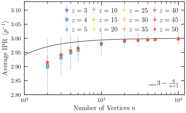
Figure 5: Graph and mode averaged inverse participation ratio vs. the number of vertices $n$ for different graph degrees $z$ (symbols). The solid line shows the finite size prediction for $\mu^{1}_{{IPR}}$ obtained by averaging over a sphere.

The solid line describes the function $\mu^{1}_{{IPR}}=3-6/(n+1)$ derived in Eq. (24) by averaging the IPR polynomial over the subsphere $S(\wp)$. There is good agreement for $n>1000$, seemingly independent of graph degree. The error bars are obtained by computing the standard deviation of ${p^{-1}}$ over all graphs in the generated set, with the largest uncertainties occurring for $z=3$. We postpone a discussion of the size and $z$-dependence of graph-to-graph fluctuations until the end of this section.

We may investigate deviations between $\expectationvalue{p^{-1}}$ and $\mu_{{IPR}}^{1}$ by defining a normalized residual

$$\Delta_{1}(z,n)=1-\frac{\expectationvalue{p^{-1}}}{\mu^{1}_{IPR}}$$ (29)

which is plotted in Fig. 6 (left) as a function of $n$ for different values of $z$.

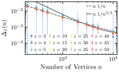
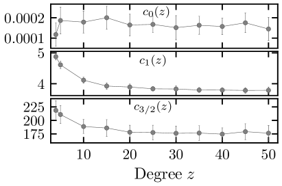
Figure 6: Left: Normalized deviation of the graph and mode averaged inverse participation ratio for the Laplacian on random regular graphs from the sphere averaged value of $\mu^{1}_{IPR}$, given in Eq. (29) in the text. Two fits to the residual data corresponding to $c_{0}+c_{1}/n$ (dashed) and $c_{3/2}/n^{3/2}$ (solid) are shown with the latter only using data with $n>1000$. Right: $z$-dependent fitting parameters are consistent with vanishing $O(1)$ corrections to to $\mu^{1}_{{IPR}}$.

The residual decays with increasing $z$ and $n$ with the correction being fit by an empirically determined function of the form $c_{0}(z)+c_{1}(z)/n$ (dashed line) where the extracted coefficients are shown in the right panel of Fig. 6. The exact diagonalization data is consistent with the absence of any $O(1)$ correction to Eq. (24) for large $z$ within errorbars, i.e. $c_{0}(z\to\infty)\to 0$. The coefficient $c_{1}(z)$ appears to decay only weakly with increasing $z$ and a $z$-dependent $1/n$ correction cannot be ruled out at the level of our statistical uncertainty for $n\leq 1000$. For $n\geq 1000$ the residual can also be described by a function of the form $c_{3/2}(z)/n^{3/2}$ as shown by the solid line in Fig. 6 (left) supporting the leading finite $n$ behavior of $\mu^{1}_{{IPR}}$.

5.2 2nd IPR moment

Next, we consider the prediction of Eq. (27) by studying the second moment of the distribution of IPR values on finite sized random regular graphs: $\expectationvalue{{(p^{-1})^{2}}}-\expectationvalue{p^{-1}}^{2}$ averaged over $N_{G}=5000$ unique graphs for $n<5000$ and $N_{G}=1000$ for $n\geq 5000$. The results are shown in Fig 7, where now deviations from the sphere-averaged value $\mu^{2}_{{IPR}}$ (included as a solid line) are observed for all values of $n$ and $z$ considered.

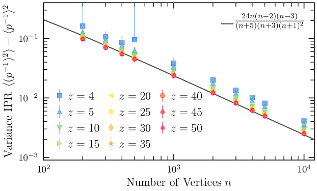
Figure 7: The graph averaged second moment of the mode averaged inverse participation ratio distribution for random regular graphs of varying degree vs. the number of vertices. The solid line shows the sphere averaged value, $\mu^{2}_{{IPR}}$.

The degree dependence is the most obvious: the exact diagonalization results are systematically larger than $\mu^{2}_{{IPR}}$ for small z, with the discrepancy decreasing as $z$ increases. We have not included data for $z=3$ in Fig. 7 as these points lie mostly off the scale and the peculiarities of this degree will be carefully investigated in the following subsection. Additionally, due to the logarithmic scale, we have only plotted errorbars showing the additive uncertainty across graphs. For $z>4$, the standard deviation is on the order of the symbol sizes.

We again define a normalized residual for the second moment:

$$\Delta_{2}(z,n)=1-\frac{\expectationvalue{(p^{-1})^{2}}-\expectationvalue{p^{-1}}^{2}}{\mu^{2}_{IPR}}$$ (30)

and the absolute value $|\Delta_{2}(z,n)|$ is plotted in Fig. 8.

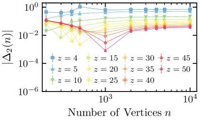
Figure 8: The normalized positive residual between the second moment of the inverse participation ratio distribution for large random regular graphs and the value obtained by averaging over a sphere. The left panel shows that the $z$ dependence of the correction can be fit via a second order polynomial in $1/z$ with an offset that persists in the $n\to\infty$ limit (right panel).

Here, the dominant deviations from the first sphere averaged value $\mu_{{IPR}}^{1}$ are degree dependent, and they can be described by a function of the form $c_{2}^{0}+c_{2}^{1}/z+c_{2}^{2}/z^{2}$. The values of the fitting constants $c_{2}^{k}$ depend on $n$, with the solid line in the left panel representing their average values for $n>1000$. Different fitting functions were investigated, including those with non-integer negative powers of $z$, but the resulting second order polynomial in $1/z$ provided the optimal value of the least square fitting $\chi^{2}$ value. The right panel of Fig. 8 shows the $n$ dependence of $\Delta_{2}$ and it appears that it remains non-zero even as $n\to\infty$. This is consistent with the fitting parameter $c^{2}_{0}$ which is finite within errorbars for all values of $z$ considered.

5.3 Effects of localized eigenvectors

We now address the issue of the large graph-to-graph variance observed around the first and second moments of the IPR distribution for small $z$. This data is displayed in Fig. 9 where the graph averaged first and second moments of the IPR distribution are shown as a function of $n$ for $z=3$.

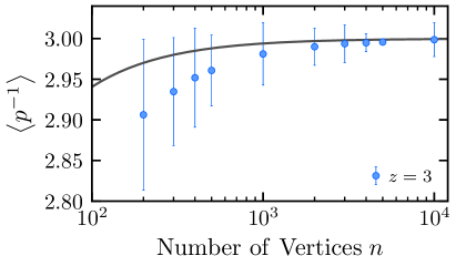
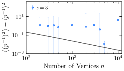
Figure 9: The first (left) and second (right) moments of the inverse participation ratio distribution vs. the number of vertices computed via exact diagonalization of $5000$ random regular graphs with degree $z=3$. The errorbars correspond to one standard deviation, and they are significantly larger than those observed for $z>3$. Solid gray lines are the predicted sphere averaged values of $\mu_{{IPR}}^{1}$ and $\mu_{{IPR}}^{2}$ defined in Eqs. (24) and (27) respectively.

The displayed errorbars correspond to one standard deviation and we observe that the effects are most pronounced for the variance of the IPR. Data points consistently fall above the sphere averaged value of $\mu_{{IPR}}^{2}$, and the mean value between graphs can vary by as much as $1000\%$. However, for both the first and second moments, the data is consistent with values of $\mu^{1}_{{IPR}}$ and $\mu^{2}_{{IPR}}$ computed using integration. The existence of a single outlying data point corresponding to $n=5000$ that is much closer to $\mu^{2}_{{IPR}}$ in the right panel of Fig. 9 is suggestive that the sample set of unique random regular graphs may not be large enough to capture the variation in the eigenvector components amongst graphs as measured by the inverse participation ratio.

To better understand the prevalence of this effect for graphs of small degree, we have exactly diagonalized the Laplacian for every one of the $\mathcal{N}_{G}=4060$ unique random regular graphs with $n=16$ and $z=3$ [46]. Analyzing the eigenvectors and computing the inverse participation ratio, we find:

$$\expectationvalue{p^{-1}} =2.4\pm 0.4$$ (31)

$$\expectationvalue{(p^{-1})^{2}}-\expectationvalue{p^{-1}}^{2} =0.95\pm 1.2\;.$$ (32)

The origin of these sizeable graph-to-graph variations is uncovered in the left panel of Fig. 10, which shows a histogram of all IPR values (excluding the Perron-Frobenius mode) for the complete graph set plotted against their corresponding eigenvalue.

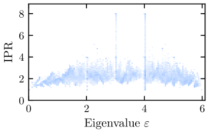
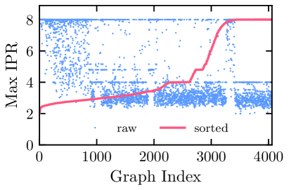
Figure 10: A histogram with shading on a logarithmic scale of the inverse participation ratio vs. eigenvalue for all 4060 random regular graphs with $n=16$ and $z=3$ (left). The right panel shows the maximum value of the inverse participation ratio across all modes for a given graph plotted as a function of a fictitious graph index. By relabeling the graph index we also include the maximum value sorted by size.

The frequency of IPR values is shown on a logarithmic color scale from light to dark, and we observe two spikes near $\varepsilon=z$ and $\varepsilon=z+1$ with the inverse participation ratio ranging up to its maximal value of $n/2=8$. In the right panel of Fig. 10 we show the maximum value of the IPR across all $n=16$ modes and find at least one value of $8$ for nearly $15\%$ of graphs in the set.

These graph realizations contain special eigenvectors $\{\boldsymbol{v}\}\subset\mathcal{E}$ of the Laplacian, with ${IPR}(\boldsymbol{{v}})=n/2$. More generally, a vector with exactly $k$ equal non-zero sites is of the form

$$v_{i}=\frac{(-1)^{q_{i}}}{\sqrt{k}}\delta_{i,i(k)}$$ (33)

where $i(k)\in\{i_{1},i_{2},\cdots,i_{k-1},i_{k}\}$ and $q_{i}\in\{0,1\}$ such that $\sum_{i(k)}(-1)^{q_{i}}=0$. Clearly this is only possible for $k=2m$ where $m\in\{1,\cdots,\lfloor n/2\rfloor\}$, with the total number of such vectors given by the multinomial coefficient

$${n\choose{m,\ m,\ n-2m}}=\frac{n!}{m!\ m!\ (n-2m)!}\;.$$

For vectors of this form, the inverse participation ratio is given by

$${IPR}(\boldsymbol{{v}})=n\sum_{i=1}^{n}|{v}_{i}|^{4}=\frac{n}{k^{2}}k=\frac{n}{k}$$ (34)

which is exactly what we observe for $k=2$. This maximal value for the IPR occurs for the most localized mode that is still compatible with orthonormality to the Perron-Frobenius eigenvector and consists of exactly two non-zero values with opposite sign. We have confirmed that such eigenvectors indeed appear in our large-$n$ graph ensembles for $z=3$. Such vectors have a maximal nodal domain count of unity [28] and we observe that almost all eigenvectors with ${IPR}(\boldsymbol{v})=n/2$ have non-zero components of opposite sign situated in vector components with consecutive indices.

The large graph-to-graph variations displayed in Fig. 9 can thus be traced back to these localized eigenvectors in combination with the prefactor of $n$ in the definition of the IPR given in Eq. (8). By averaging over the sphere, we found in Eq. (24) that $\mu_{{IPR}}^{1}\sim 3$ for $n\gg 1$. However as just demonstrated, localized eigenvectors can contribute IPR values of $\mathrm{O}(n)$ to the first moment. This implies that the variance around the mean could contain dominant terms scaling like $n^{2}$ which will always have an effect when averaging over a finite number of large graphs.

6 Discussion

In this paper we have investigated the first and second moments of the distribution of the inverse participation ratio for all eigenvectors of the discrete Laplacian on finite size random regular graphs. By exactly diagonalizing large ensembles of graphs of up to $n=10000$ vertices we find that the first moment of the inverse participation ratio approaches a constant of order unity $\lim_{n\to\infty}\expectationvalue{p^{-1}}=3$ for all values of $z$. This result can be understood in terms of an analytically determined value for the average inverse participation ratio $\mu_{{IPR}}^{1}=3-6/(n+1)$ obtained by averaging a fourth order polynomial corresponding to the IPR over the sphere $S(\wp)$ with uniform probability measure. We take this agreement as additional evidence that that the average eigenvector of the Laplacian on random regular graphs is delocalized, with its components tending towards being independent and identically distributed Gaussian random variables. For smaller values of $n$ that do not necessarily satisfy the constraint $n^{\delta}\leq z\leq n^{2/3-\delta}$ for $\delta>0$ [32], we observe deviations from $\mu_{{IPR}}^{1}$ at $O(1/n)$ that could be potentially useful when quantifying the distance from uniformity for a given set of random regular graph eigenvectors. The methodology used here to average the IPR polynomial over the hypersphere with constant probability could be employed to study other observables of physical interest on random graphs when $n$ is large.

For the variance of the inverse participation ratio computed over all modes, we have again compared our exact random regular graph eigenvectors with an analytical result from continuous averaging over $S(\wp)$ with uniform measure where we find $\mu_{{IPR}}^{2}=24n(n-2)(n-3)/[(n+5)(n+3)(n+1)^{2}]$. Here we observe weaker agreement that now strongly depends on the graph degree. This discrepancy appears to persist even in the limits $z,n\to\infty$. When computing the standard deviation of the IPR over an ensemble of up to $5000$ random regular graphs, we find that for small values of the graph degree $z$, large fluctuations between graph eigenvectors can cause variations in the first and second moments as large as $1000\%$. By analyzing the complete set of graphs for $z=3$ and $n=16$ we have shown that such deviations may arise from graphs where the Laplacian has localized eigenvectors consisting of only a few non-zero elements and thus IPR values of $n/2$. Although we have no proof that these vectors appear as eigenvectors of the Laplacian for finite size random regular graphs in general, we have demonstrated that there are factorially many such eigenvectors that are orthonormal to the Perron-Frobenius mode.

In general, the large but finite ensemble size of random regular graphs we analyze is much smaller than the total number of random regular graphs, which is known [34] to asymptotically grow exponentially with $n$. Hence, the fact that the standard deviation in the mean and variance of the inverse participation ratio for large $n$ and $z$ appear to be small is likely due to our samples of random regular graphs not being fully representative of the eigenvector variation which exists.

As $z$ and $n$ increase, extremely large ensembles of graphs need to be studied in order to to balance the dominant effects of localized modes, especially for non-linear observables. Thus, any observed deviation of the 2nd moment of the IPR from its uniform value for a given set of finite size graphs could be employed as a proxy for the representative suitability of the sampled set when $n$ is large. This may may have practical implications for studying physical models with observables computed on regular graphs.

It would be interesting to explore this issue further, although considerable computational resources would have to be employed to diagonalize large numbers of graph Laplacians for $n\gg 1$. Determining the combinatorial, physical, and theoretical significance of these localized eigenvectors is thus left as a topic of future work.

7 Acknowledgements

The authors thank R. Bauerschmidt for help clarifying current results on the distribution of eigenvector components of random regular graphs. A.D. is deeply indebted to Z. Tešanović, for diverse and stimulating discussions that ultimately spawned my interest in graph theory and lead to this collaborative work. A.D. also thanks T. Lakoba for his insights into high dimensional coordinate transformations. T.C. is grateful to M. Shah, for lively and informative numerical linear algebra conversations and to B. H. Lee for clarification of key statistical notions. This research was supported in part by the National Science Foundation (NSF) under award No. DMR-1553991 (A.D.). All computations were performed on the Vermont Advanced Computing Core supported in part by NSF award No. OAC-1827314.

Appendix A Averages of Monomials on the Sphere

This appendix contains results of averaging monomials over the uniform distribution on $S(\boldsymbol{e}_{n})$ necessary for the integral calculations of Section 4. Note that in our case, the polynomial ${IPR}(Q^{-1}\boldsymbol{y})$ consists of monomials in the variables $y_{1},\ldots,y_{n-1}$ since $y_{n}=0$. Theorem 15 guarantees that the integral of a monomial is non-zero precisely when its variables have even exponents, and as such, we give values in only this case.

When performing the first moment calculations we apply Theorem 15 to two distinct monomial types. The monomial $y_{i}^{4}$ has $a_{i}=4$ for a fixed $i$ and $a_{j}=0$ for all $j\neq i$, while the monomial $y_{i}^{2}y_{j}^{2}$ has $a_{i}=a_{j}=2$ and $a_{k}=0$ for $k\neq i,j$. In the first case, we therefore have $b_{i}=5/2$ for a single $i$ and $b_{j}=1/2$ for $j\neq i$. In the second case, $b_{i}=b_{j}=3/2$ and $b_{k}=1/2$ for $k\neq i,j$. For $y_{k}^{4}$ we average over $S(\boldsymbol{e}_{n})$ and find:

$$\expectationvalue{y_{k}^{4}}_{S(\boldsymbol{e}_{n})} =\int_{S(\boldsymbol{e}_{n})}y_{k}^{4}\,P(\boldsymbol{y})\,d\sigma(\boldsymbol{e}_{n})$$

$$=\frac{\Gamma\quantity(\frac{n-1}{2})}{2\pi^{(n-1)/2}}\frac{2\Gamma\quantity(\frac{5}{2})\left[\Gamma\quantity(\frac{1}{2})\right]^{n-2}}{\Gamma\quantity(\frac{n+3}{2})}$$

$$=\frac{3}{4}\frac{\Gamma\quantity(\frac{n-1}{2})}{\Gamma\quantity(\frac{n+3}{2})}$$ (35)

This result along with the similarly computed $\expectationvalue{y^{2}y^{2}}$ term are gathered in Table 1.

Average:	$\expectationvalue{y_{k}^{4}}_{S(\boldsymbol{e}_{n})}$	$\expectationvalue{y_{k}^{2}y_{\ell}^{2}}_{S(\boldsymbol{e}_{n})}$
Value:	$\displaystyle\frac{3}{4}\frac{\Gamma\quantity(\frac{n-1}{2})}{\Gamma\quantity(\frac{n+3}{2})}$	$\displaystyle\frac{1}{4}\frac{\Gamma\quantity(\frac{n-1}{2})}{\Gamma\quantity(\frac{n+3}{2})}$

Table 1: The average values of the degree four monomials with even exponents in $y_{1},\ldots,y_{n-1}$ taken over the domain $S(\boldsymbol{e}_{n})$ with uniform probability.

A similar analysis of the five monomial types appearing in the second moment’s polynomial $[{IPR}(Q^{-1}\boldsymbol{y})]^{2}$ yields non-zero averages for those monomials of total degree eight which we list in Table 2.

Average:	$\expectationvalue{y_{k}^{8}}_{S(\boldsymbol{e}_{n})}$	$\expectationvalue{y_{k}^{6}y_{\ell}^{2}}_{S(\boldsymbol{e}_{n})}$	$\expectationvalue{y_{k}^{4}y_{\ell}^{4}}_{S(\boldsymbol{e}_{n})}$	$\expectationvalue{y_{k}^{4}y_{\ell}^{2}y_{m}^{2}}_{S(\boldsymbol{e}_{n})}$	$\expectationvalue{y_{k}^{2}y_{\ell}^{2}y_{m}^{2}y_{p}^{2}}_{S(\boldsymbol{e}_{n})}$
Value:	$\displaystyle\frac{105}{16}\frac{\Gamma\quantity(\frac{n-1}{2})}{\Gamma\quantity(\frac{n+7}{2})}$	$\displaystyle\frac{15}{16}\frac{\Gamma\quantity(\frac{n-1}{2})}{\Gamma\quantity(\frac{n+7}{2})}$	$\displaystyle\frac{9}{16}\frac{\Gamma\quantity(\frac{n-1}{2})}{\Gamma\quantity(\frac{n+7}{2})}$	$\displaystyle\frac{3}{16}\frac{\Gamma\quantity(\frac{n-1}{2})}{\Gamma\quantity(\frac{n+7}{2})}$	$\displaystyle\frac{1}{16}\frac{\Gamma\quantity(\frac{n-1}{2})}{\Gamma\quantity(\frac{n+7}{2})}$

Table 2: The average values of the degree eight monomials with even exponents in $y_{1},\ldots,y_{n-1}$ taken over the domain $S(\boldsymbol{e}_{n})$ with uniform probability.

We now discuss each of the denominators appearing in these monomial integral calculations, and do so taking the value $\Gamma\quantity(\frac{n-1}{2})$ into account. This quantity is the numerator of the probability $P(\boldsymbol{x})$ of choosing points uniformly from the sphere and is a prefactor of each moment calculation. A closed form for the first and second IPR moments therefore depends on our ability to simplify several $n$-dependent ratios.

For the first moment, the total degree of the monomials is four, giving the denominator of Theorem 15 a value of $\Gamma(\frac{n+3}{2})$. Hence, we seek a closed form for ${\Gamma(\frac{n-1}{2})}/{\Gamma(\frac{n+3}{2})}$. For a positive integer $k$, the Gamma function takes the values $\Gamma(k)=(k-1)!$ and $\Gamma(k+\frac{1}{2})=(k-\frac{1}{2})\cdots(\frac{1}{2})\sqrt{\pi}$ so that we have the following derivations:

If $n-1=2k$ is even, then

$$\frac{\Gamma(\frac{n-1}{2})}{\Gamma(\frac{n+3}{2})}=\frac{(k-1)!}{(k+1)!}=\frac{1}{(\frac{n+1}{2})(\frac{n-1}{2})}=\frac{4}{(n+1)(n-1)}.$$ (36)

On the other hand, if $n-1$ is odd, then $n-1=2k+1$ for some $k$ and

$$\frac{\Gamma(\frac{n-1}{2})}{\Gamma(\frac{n+3}{2})}=\frac{(k-\frac{1}{2})\cdots(\frac{1}{2})\sqrt{\pi}}{(k+\frac{3}{2})(k+\frac{1}{2})\cdots(\frac{1}{2})\sqrt{\pi}}=\frac{4}{(2k+3)(2k+1)}=\frac{4}{(n+1)(n-1)}.$$ (37)

The second moment calculation contains only monomials of total degree eight, so that the denominator of Theorem 15 is $\Gamma(\frac{n+7}{2})$. In a fashion similar to the derivation above, we give an alternate form for the fraction ${\Gamma(\frac{n-1}{2})}/{\Gamma(\frac{n+7}{2})}$.

When $n-1=2k$ is even, we have

$$\frac{\Gamma(\frac{n-1}{2})}{\Gamma(\frac{n+7}{2})}=\frac{(k-1)!}{(k+3)!}=\frac{1}{(k+3)(k+2)(k+1)(k)}=\frac{16}{(n+5)(n+3)(n+1)(n-1)}.$$ (38)

On the other hand, for odd $n-1=2k+1$,

$$\frac{\Gamma(\frac{n-1}{2})}{\Gamma(\frac{n+7}{2})}=\frac{\left(k-\frac{1}{2}\right)\left(k-\frac{3}{2}\right)\cdots\left(\frac{1}{2}\right)\sqrt{\pi}}{\left(k+\frac{7}{2}\right)\left(k+\frac{5}{2}\right)\left(k+\frac{3}{2}\right)\cdots\left(\frac{1}{2}\right)\sqrt{\pi}}=\frac{16}{(n+5)(n+3)(n+1)(n-1)}.$$ (39)

Appendix B Evaluation of $Q$ Summations

In this appendix we provide details on the evaluation of the summations over the components of the rotation matrix $Q$ given in Eq. (21) that appear in the expressions for the first (Eq. (23)) and second (Eq. (25)) moments of the of the inverse participation ratio. These evaluations are performed by first noting that all such powers of $Q$ only appear with the first index smaller than $n$ and in this restricted case we can write:

$$\left(Q_{ij}\right)^{s}=\frac{1}{(n+\sqrt{n})^{s}}\left[(-1)^{s}+\alpha_{s}(n)\delta_{nj}+\beta_{s}(n)\delta_{ij}\right]$$ (40)

where $\alpha_{s}(n)$ and $\beta_{s}(n)$ are power dependent functions of $n$ that are listed in Table 3 and we have used the fact that $\delta_{ij}^{s}=\delta_{ij}$ and $\delta_{ij}^{s}\delta_{n,j}^{s^{\prime}}=0$ $\forall s,s^{\prime}\geq 1$ since $i<n$.

$s$	$\alpha_{s}(n)$	$\beta_{s}(n)$
1	$-\sqrt{n}$	$n+\sqrt{n}$
2	$n+2\sqrt{n}$	$(n-1)(n+2\sqrt{n})$
3	$-\sqrt{n}\left(3+3\sqrt{n}+n\right)$	$(n+\sqrt{n})(3-3\sqrt{n}-2n+2n^{3/2}+n^{2})$
4	$(n+2\sqrt{n})(2+2\sqrt{n}+n)$	$\!\begin{aligned} &(n-1)(n+2\sqrt{n})\\ &\;\times(n^{2}+2n^{3/2}-n-2\sqrt{n}+2)\end{aligned}$
6	$\!\begin{aligned} &(n+2\sqrt{n})(1+\sqrt{n}+n)\\ &\;\times(3+3\sqrt{n}+n)\end{aligned}$	$\!\begin{aligned} &(n+2\sqrt{n})(n-1)(1-\sqrt{n}+2n^{3/2}+n^{2})\\ &\;\times(3-3\sqrt{n}-2n+2n^{3/2}+n^{2})\end{aligned}$
8	$\!\begin{aligned} &(n+2\sqrt{n})(2+2\sqrt{n}+n)\\ &\;\times(2+4\sqrt{n}+6n+4n^{3/2}+n^{2})\end{aligned}$	$\!\begin{aligned} &(n+2\sqrt{n})(n-1)\\ &\;\times(2-2\sqrt{n}-n+2n^{3/2}+n^{2})\\ &\;\times(2-4\sqrt{n}+2n+8n^{3/2}-5n^{2}\\ &\qquad\;-\ 8n^{5/2}+2n^{3}+4n^{7/2}+n^{4})\end{aligned}$

Table 3: Expressions for $\alpha_{s}(n)$ and $\beta_{s}(n)$ appearing as coefficients of Kronecker $\delta$-functions when evaluating powers of the components of the rotation matrix $(Q_{ij})^{s}$ where $i<n$ in Eq. (40).

B.1 1st IPR moment

We begin by using Eq. (40) to perform the double and triple summations appearing in the expression for the first moment of the inverse participation ratio in Eq. (23).

$$\sum_{i=1}^{n}\sum_{k=1}^{n-1}Q_{ki}^{4} =\frac{1}{(n+\sqrt{n})^{4}}\sum_{i=1}^{n}\sum_{k=1}^{n-1}\left[1+\alpha_{4}(n)\delta_{ni}+\beta_{4}(n)\delta_{ki}\right]$$

$$=\frac{1}{(n+\sqrt{n})^{4}}\left[n(n-1)+\alpha_{4}(n)(n-1)+\beta_{4}(n)(n-1)\right]$$

$$=\frac{n-1}{(n+\sqrt{n})^{4}}\left[n+\alpha_{4}(n)+\beta_{4}(n)\right]$$ (41)

and using the values of $\alpha_{4}(n)$ and $\beta_{4}(n)$ in Table 3 we find

$$\sum_{i=1}^{n}\sum_{k=1}^{n-1}Q_{ki}^{4}=n-\frac{29+30\sqrt{n}+5n}{(1+\sqrt{n})^{2}}+\frac{24}{\sqrt{n}}-\frac{9}{n}.$$ (42)

Now, dropping the explicit $n$ dependence of the $\alpha_{s}$ and $\beta_{s}$ functions for simplicity, the triple summation may be performed in a similar manner:

$$\sum_{i=1}^{n}\sideset{}{{}^{\prime}}{\sum}_{k,\ell}^{n-1}Q_{ki}^{2}Q_{\ell i}^{2} =\frac{1}{(n+\sqrt{n})^{4}}\sum_{i=1}^{n}\sum_{k\neq\ell}^{n-1}\left(1+\alpha_{2}\delta_{ni}+\beta_{2}\delta_{ki}\right)\left(1+\alpha_{2}\delta_{ni}+\beta_{2}\delta_{\ell i}\right)$$

$$=\frac{1}{(n+\sqrt{n})^{4}}\sum_{k\neq\ell}^{n-1}\left[(1+\alpha_{2})^{2}+\sum_{i=1}^{n-1}(1+\beta_{2}\delta_{ki})(1+\beta_{2}\delta_{\ell i})\right]$$

$$=\frac{1}{(n+\sqrt{n})^{4}}\sum_{k\neq\ell}^{n-1}\left[(1+\alpha_{2})^{2}+n-1+2\beta_{2}\right]$$

$$=\frac{(n-1)(n-2)}{(n+\sqrt{n})^{4}}\left[(1+\alpha_{2})^{2}+n-1+2\beta_{2}\right]$$

$$=\frac{(\sqrt{n}-1)(3\sqrt{n}+5)(n-2)}{n(\sqrt{n}+1)^{2}},$$ (43)

where we have used $\alpha_{2}(n)$ and $\beta_{2}(n)$ from Table 3.

B.2 2nd IPR moment

There are seventeen individual summations appearing in the expression for the average of the square of the inverse participation ratio over the sphere given in Eq. (25) and we will include the details of only a representative sample here. All can be performed using similar techniques employing Eq. (40) and Table 3 and we begin with the sum over the components of $Q^{8}$ which can be evaluated in exact analogy with Eq. (41):

$$\sum_{k=1}^{n-1}\sum_{i=1}^{n}Q_{ki}^{8} =\frac{1}{(n+\sqrt{n})^{8}}\sum_{k=1}^{n-1}\sum_{i=1}^{n}\left[1+\alpha_{8}\delta_{ni}+\beta_{8}\delta_{ki}\right]$$

$$=\frac{\sqrt{n}-1}{(1+\sqrt{n})^{6}n^{3}}\left(49+7\sqrt{n}-7n+119n^{3/2}+21n^{2}-133n^{5/2}+9n^{3}\right.$$

$$\left.\qquad\qquad\quad+\ 111n^{7/2}+n^{4}-57n^{9/2}-13n^{5}+13n^{11/2}+7n^{6}+n^{13/2}\right).$$

The next novel term includes $Q^{6}$ which appears as the third summation and is evaluated in a similar method as in Eq. (43) albeit with the modification that it involves the product of two different powers of $Q$:

$$\sideset{}{{}^{\prime}}{\sum}_{k,\ell}^{n-1}\sum_{i=1}^{n}Q_{ki}^{6}Q_{\ell i}^{2} =\frac{1}{(n+\sqrt{n})^{8}}\sum_{k\neq\ell}^{n-1}\sum_{i=1}^{n}\left(1+\alpha_{6}\delta_{ni}+\beta_{6}\delta_{ki}\right)\left(1+\alpha_{2}\delta_{ni}+\beta_{2}\delta_{\ell i}\right)$$

$$=\frac{1}{(n+\sqrt{n})^{8}}\sum_{k\neq\ell}^{n-1}\left[(1+\alpha_{6})(1+\alpha_{2})+\sum_{i=1}^{n-1}(1+\beta_{6}\delta_{ki})(1+\beta_{2}\delta_{\ell i})\right]$$

$$=\frac{(n-1)(n-2)}{(n+\sqrt{n})^{8}}\left[(1+\alpha_{6})(1+\alpha_{2})+n-1+\beta_{6}+\beta_{2}\right]$$

$$=\frac{\left(\sqrt{n}-1\right)(-2+n)}{\left(1+\sqrt{n}\right)^{6}n^{3}}\left(37+31\sqrt{n}+10n+40n^{3/2}+29n^{2}-15n^{5/2}\right.$$

$$\left.\qquad\qquad\qquad\qquad-14n^{3}+4n^{7/2}+5n^{4}+n^{9/2}\right).$$

The final type of term contains mixed second indices between the different rotation matrix powers and we consider the thirteenth sum in Eq. (25) as a representative of this set. The strategy is the same for all such terms and involves performing the inner summation by extracting the terms with $i=n$ and $j=n$ and performing the summations over $j$ and $i$, then breaking the remaining restricted sum over $i\neq j\leq n-1$ into the difference of an unrestricted sum over all values of $i,j\leq n-1$ and one with $i=j\leq n-1$. We have

$$(n+\sqrt{n})^{8}\sum_{i\neq j}^{n}Q_{ki}^{3}Q_{\ell i}Q_{kj}Q_{\ell j}Q_{mj}^{2}$$

$$\;\;=\left(-1+\alpha_{3}\right)\left(-1+\alpha_{1}\right)\sum_{j=1}^{n-1}\left(-1+\beta_{1}\delta_{kj}\right)\left(-1+\beta_{1}\delta_{\ell j}\right)\left(1+\beta_{2}\delta_{mj}\right)$$

$$\;\;\quad+\;\left(-1+\alpha_{1}\right)^{2}\left(1+\alpha_{2}\right)\sum_{i=1}^{n-1}\left(-1+\beta_{3}\delta_{ki}\right)\left(-1+\beta_{3}\delta_{\ell i}\right)$$

$$\;\;\quad+\;\sum_{i=1}^{n-1}\left(-1+\beta_{3}\delta_{ki}\right)\left(-1+\beta_{1}\delta_{\ell i}\right)\sum_{j=1}^{n-1}\left(-1+\beta_{1}\delta_{kj}\right)\left(-1+\beta_{1}\delta_{\ell j}\right)\left(1+\beta_{2}\delta_{mj}\right)$$

$$\;\;\quad-\;\sum_{i=1}^{n-1}\left(-1+\beta_{3}\delta_{ki}\right)\left(-1+\beta_{3}\delta_{\ell i}\right)^{2}\left(-1+\beta_{1}\delta_{ki}\right)\left(1+\beta_{2}\delta_{mi}\right)$$

$$\;\;=\left[(-1+\alpha_{1})(-1+\alpha_{3})(n-1-2\beta_{1}+\beta_{2})+(1+\alpha_{2})(-1+\alpha_{1})^{2}(n-1-\beta_{1}-\beta_{3})\right.$$

$$\;\;\;\;\quad\left.+\;(n-1-\beta_{1}-\beta_{3})(n-1-2\beta_{1}+\beta_{2})-(n-1-3\beta_{1}+\beta_{2}-\beta_{3}+\beta_{1}\beta_{2}+\beta_{1}^{2})\right]$$

and putting everything together:

$$\sideset{}{{}^{\prime}}{\sum}_{k,\ell,m}^{n-1}\sideset{}{{}^{\prime}}{\sum}_{i,j}^{n}Q_{ki}^{3}Q_{\ell i}Q_{kj}Q_{\ell j}Q_{mj}^{2} =\frac{(1-\sqrt{n})(n-2)(n-3)}{\left(1+\sqrt{n}\right)^{6}n^{3}}\left(29+39\sqrt{n}+4n-28n^{3/2}\right.$$

$$\;\;\quad\qquad\qquad\qquad\left.-\ 12n^{2}+12n^{5/2}+10n^{3}+2n^{7/2}\right).$$

References

- [1] Essam J W 1971 Dis. Math. 1 83
- [2] Anderson P W 1958 Phys. Rev. 109 1492
- [3] Abou-Chacra R, Thouless D J and Anderson P W 1973 J. Phys. C: Solid State 6 1734
- [4] Georges A, Kotliar G, Krauth W and Rozenberg M J 1996 Rev. Mod. Phys. 68 13
- [5] Lichtenstein A I and Katsnelson M I 2000 Phys. Rev. B 62 R9283
- [6] Hastings M 2003 Phys. Rev. Lett. 90 148702
- [7] Burioni R, Cassi D and Destri C 2000 Phys. Rev. Lett. 85 1496
- [8] Laumann C R, Parameswaran S A and Sondhi S L 2009 Phys. Rev. B 80 144415
- [9] Murray J, Del Maestro A and Tešanović Z 2012 Phys. Rev. B 85
- [10] Burioni R, Cassi D, Rasetti M, Sodano P and Vezzani A 2001 J. Phys. B: Atom., Mol. Opt. Phys. 34 4697
- [11] Hagberg A A, Schult D A and Swart P J 2008 Exploring network structure, dynamics, and function using NetworkX Proceedings of the 7th Python in Science Conference (SciPy2008) ed Varoquaux G, Vaught T and Millman J p 11
- [12] Steger A and Wormald N 1999 Comb. Prob. Comput. 8 377
- [13] Kim J H and Vu V H 2003 Proceedings of the thirty-fifth ACM symposium on Theory of computing
- [14] Hoory S, Linial N and Wigderson A 2006 B. Am. Math. Soc. 43 439
- [15] Kesten H 1959 Trans. Am. Math. Soc. 92 336
- [16] McKay B D 1981 Lin. Alg. Appl. 40 IS - 203
- [17] Tran L V, Vu V H and Wang K 2013 Ran. Struct. Alg. 42 110
- [18] Dumitriu I and Pal S 2012 Ann. Probab. 40 2197
- [19] Metz F L, Parisi G and Leuzzi L 2014 Phys. Rev. E 90 052109
- [20] Bauerschmidt R, Huang J and Yau H T 2016 arXiv (Preprint 1609.09052)
- [21] Bauerschmidt R, Knowles A and Yau H T 2017 Commun. Pure Appl. Math 70 1898
- [22] Deift P 2007 Universality for mathematical and physical systems International Congress of Mathematicians. Vol. I (Eur. Math. Soc., Zürich) p 125
- [23] Jakobson D, Miller S D, Rivin I and Rudnick Z 1999 Eigenvalue Spacings for Regular Graphs Emerging Applications of Number Theory (New York, NY: Springer) pp 317–327
- [24] Oren I and Smilansky U 2010 J. Phys. A: Math. Theor. 43 225205
- [25] Bauerschmidt R, Huang J, Knowles A and Yau H T 2017 Ann. Probab. 45 3626–3663
- [26] Friedman J 1993 Duke Math. J. 69 487
- [27] Elon Y 2008 J. Phys. A: Math. Theor. 41 435203
- [28] Dekel Y, Lee J R, Linial N and Linial N 2010 Ran. Struct. Alg. 39 39
- [29] Kabashima Y and Takahashi H 2012 J. Phys. A: Math. Theor. 45 325001
- [30] Brooks S and Lindenstrauss E 2012 Isr. J. Math. 193 1
- [31] Geisinger L 2015 J. Spectr. Theor. 5 783
- [32] Bourgade P, Huang J and Yau H T 2017 Electron. J. Probab. 22 64
- [33] Backhausz A and Szegedy B 2016 arXiv (Preprint 1607.04785)
- [34] Bollobás B 1980 Euro. J. Comb. 1 311
- [35] 2018 OEIS Foundation Inc., The On-Line Encyclopedia of Integer Sequences, http://oeis.org/A002851
- [36] Füredi Z and Komlós J 1981 Combinatorica 1 233
- [37] Bell R J and Dean P 1970 Discuss. Faraday Soc. 50 55
- [38] Visscher W M 1972 J. Non-Cryst. Sol. 8-10 477
- [39] Cizeau P and Bouchaud J 1994 Phys. Rev. E 50 1810
- [40] Cavagna A, Giardina I and Parisi G 1999 Phys. Rev. Lett. 83 108
- [41] Metz F L, Neri I and Bollé D 2010 Phys. Rev. E 82 031135
- [42] Slanina F 2012 Euro. Phys. J. B 85 1
- [43] Cramér H 1999 Mathematical methods of statistics Princeton Landmarks in Mathematics (Princeton University Press, Princeton, NJ) ISBN 0-691-00547-8 reprint of the 1946 original
- [44] Muller M E 1959 Commun. ACM 2 19–20
- [45] Folland G B 2001 Am. Math. Mon. 108 446
- [46] Meringer M 1999 J. Graph Th. 30 137