The Neutral Hydrogen Cosmological Mass Density at $\mathbf{z=5}$

Abstract

We present the largest homogeneous survey of $z>4.4$ damped $\rm Ly\alpha$ systems (DLAs) using the spectra of 163 QSOs that comprise the Giant Gemini GMOS (GGG) survey. With this survey we make the most precise high-redshift measurement of the cosmological mass density of neutral hydrogen, $\rm\Omega_{\rm HI}$. At such high redshift important systematic uncertainties in the identification of DLAs are produced by strong intergalactic medium absorption and QSO continuum placement. These can cause spurious DLA detections, result in real DLAs being missed, or bias the inferred DLA column density distribution. We correct for these effects using a combination of mock and higher-resolution spectra, and show that for the GGG DLA sample the uncertainties introduced are smaller than the statistical errors on $\rm\Omega_{\rm HI}$. We find $\rm\Omega_{\rm HI}=0.98^{+0.20}_{-0.18}\times 10^{-3}$ at $\langle z\rangle=4.9$, assuming a 20% contribution from lower column density systems below the DLA threshold. By comparing to literature measurements at lower redshifts, we show that $\rm\Omega_{\rm HI}$ can be described by the functional form $\Omega_{\rm HI}(z)\propto(1+z)^{0.4}$. This gradual decrease from $z=5$ to $0$ is consistent with the bulk of H i gas being a transitory phase fuelling star formation, which is continually replenished by more highly-ionized gas from the intergalactic medium, and from recycled galactic winds.

1 Introduction

The neutral hydrogen mass density of the universe, $\rm\Omega_{\rm HI}$, is an important cosmological observable. It determines the precision with which cosmological parameters can be constrained by observations of the H i intensity power spectrum (e.g. Barkana & Loeb, 2007; Chang et al., 2008; Wyithe & Loeb, 2008; Padmanabhan et al., 2015), and we expect its evolution to be linked to the cosmic star formation history. The main contributor to $\rm\Omega_{\rm HI}$ is high column density, predominantly neutral gas clouds (e.g. O’Meara et al., 2007; Zafar et al., 2013), self-shielded from ionizing radiation and therefore likely fuel for future star formation (e.g. Wolfe et al., 2005). Thus tracing the evolution of $\rm\Omega_{\rm HI}$ from the end of reionization, through the epoch of the cosmic star formation peak at $z\sim 2$ to the present day is of central importance to our understanding of galaxy formation. It also provides an excellent integral constraint against which theoretical models of galaxy formation can be tested.

At redshift $<0.3$, H i 21 cm emission can be used to measure $\rm\Omega_{\rm HI}$ either directly or by stacking analyses (e.g. Zwaan et al., 2005; Martin et al., 2010). At higher redshifts, where emission is too weak to be detected with current facilities, $\rm\Omega_{\rm HI}$ can instead be inferred from the incidence rate of damped $\rm Ly\alpha$ systems (DLAs, defined as absorption systems with ${\it N}_{\mathrm{HI}}\geq 20.3$ cm^-2), which trace the bulk of neutral gas in the universe (Prochaska et al., 2005). These systems are detected in absorption in the spectra of background QSOs, and their characteristic damping wings allow column densities to be measured even at low spectral resolution.

Early DLA surveys at $2<z<4$, which were typically comprised of a few hundred QSOs and assumed a cosmological deceleration parameter $q_{0}=0.5$ or $0$, suggested that the gas mass density in DLAs may have been sufficient to produce most of the stars seen in the local universe (Lanzetta et al., 1991; Wolfe et al., 1995; Storrie-Lombardi et al., 1996). However, a change to a modern concordance cosmology revealed that DLAs at $z\sim 3$ contain $<50$ percent of the present day mass density in stars (e.g. Storrie-Lombardi & Wolfe, 2000; Péroux et al., 2005, see also Section 5.2). In addition, recent DLA surveys at $2<z<4$ using more than 10,000 QSOs assembled from the Sloan Digital Sky Survey (SDSS) (Prochaska & Herbert-Fort, 2004; Prochaska et al., 2005; Prochaska & Wolfe, 2009; Noterdaeme et al., 2009, 2012) have shown that there is very little evolution in the H i mass density from $z=3$ to the present day. This is starkly at odds with the strong evolution in the star formation rate over the same period (e.g. Madau & Dickinson, 2014). One view is that H i represents a transitory phase fuelling star formation (e.g. Prochaska et al., 2005; Davé et al., 2013), which is continually replenished by more highly ionized gas from either the intergalactic medium (IGM) or recycled galactic outflows.

While it is important to constrain $\rm\Omega_{\rm HI}$ across the whole of cosmic history, it is of particular interest at the highest redshifts. Rafelski et al. (2014) report a decrease in the metal mass density in damped $\rm Ly\alpha$ systems from $z=5$ to $4.5$, hinting at an abrupt change in the enrichment of H i gas past $z=5$. This may be caused by a change in the population of objects containing neutral hydrogen, which could be accompanied by a similarly abrupt evolution in $\rm\Omega_{\rm HI}$. Moreover, since massive stars in galaxies are believed to have reionized the Universe (e.g. Bouwens et al., 2012), it is important to track the evolution of the fuel for star formation up to the epoch of reionization. However, it is a challenge to assemble the large sample of high-redshift QSO spectra necessary for a $z>4.5$ DLA survey. The decline in the QSO space density at $z>3$ means that relatively few redshift $>4.4$ QSOs were observed by the SDSS, and those that were typically have too low a S/N to reliably identify DLAs. For example, Rafelski et al. (2012, 2014) find a misidentification rate of 26% for DLA candidates from SDSS DR5 at $z>4$, and of 97% for candidates from DR9 at $z>4.7$. For this reason smaller DLA surveys have been performed at higher redshift, often using higher resolution spectra to make robust identifications of DLAs. Péroux et al. (2003), Guimarães et al. (2009) and Songaila & Cowie (2010) have all presented measurements of $\rm\Omega_{\rm HI}$ at $z>4.5$. Songaila & Cowie (2010, hereafter S10) give a cumulative result including data from all these previous studies, and this represents the highest redshift measurement of $\rm\Omega_{\rm HI}$ to date. They use a sample of 19 QSOs with emission redshifts $>4.5$, and their measurement hints at a possible downturn in $\rm\Omega_{\rm HI}$ at $z\geq 4$, but the uncertainties from sample variance at $z>4.3$ are large.

Here we measure $\rm\Omega_{\rm HI}$ as traced by DLAs at $3.5<z<5.4$ using a homogeneous sample of 163 QSOs with emission redshifts between 4.4 and 5.4. This represents an increase in redshift path of a factor of eight over S10 at $z>4.5$. Identifying DLAs becomes increasingly difficult at higher redshift, as H i absorption from the highly-ionized intergalactic medium (IGM) becomes more severe, and blending with strong systems below the DLA threshold can cause misidentification of DLAs. Therefore we carefully check for systematic misidentifications in our sample using both mock spectra and higher resolution spectra of DLA candidates. More than 70% of our DLA candidates (and $>85\%$ at $z>4.5$) have been observed at higher resolution (Rafelski et al., 2012, 2014), allowing us to confirm their ${\it N}_{\mathrm{HI}}$ despite the increased IGM blending at high redshift.

This paper is structured as follows. In Section 2 we describe the QSO spectra used for the analysis. Section 3 describes the formalism used to derive $\rm\Omega_{\rm HI}$ from our observations and Section 4 describes our method for measuring the DLA incidence rate, accounting for systematic effects. Section 5 describes our main result, a measurement of the neutral hydrogen mass density at $z=5$, and discusses its implications. Section 6 summarises our conclusions. We assume a flat $\Lambda$CDM cosmology, with H${}_{0}=70\,\rm km\,s^{-1}$Mpc^-1, $\Omega_{m,0}=0.3$ and $\Omega_{\Lambda,0}=0.7$. All distances are comoving unless stated otherwise. The data and code used for this paper are available at https://github.com/nhmc/GGG_DLA.

2 Data

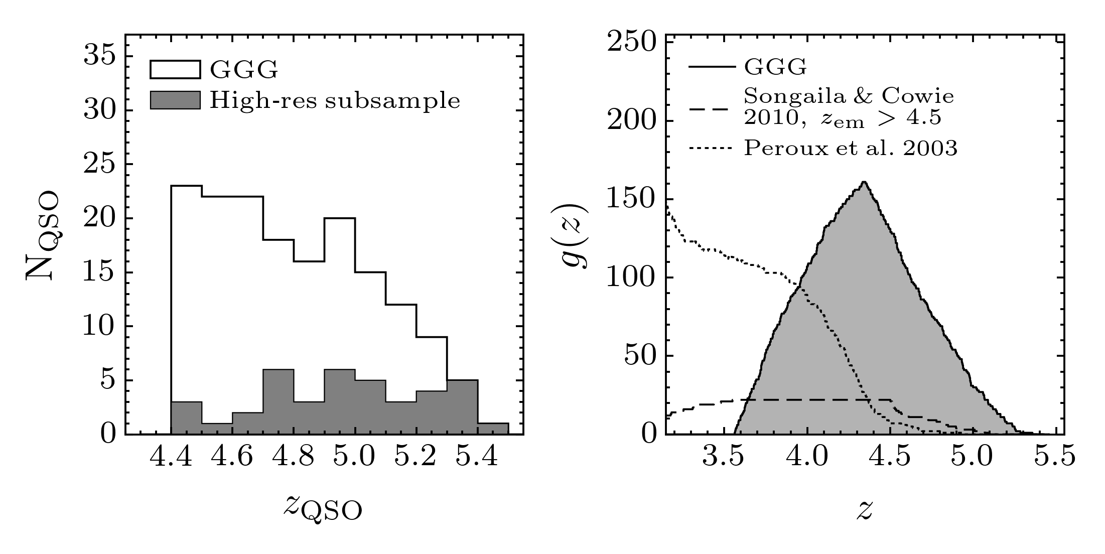
Our main data sample consists of GMOS spectra for the 163 QSOs which comprise the Giant Gemini GMOS (GGG) survey (Worseck et al., 2014). The QSOs were taken from the SDSS and all have emission redshifts $4.4<z<5.4$. At these emission redshifts, the QSO sightlines are likely unbiased regarding the number density of DLAs, unlike sightlines with $2.7<z_{\mathrm{em}}<3.6$ (Prochaska et al., 2009; Worseck & Prochaska, 2011; Fumagalli et al., 2013). We also use a smaller sample of 59 QSOs with higher resolution spectra, listed in Table 3. In contrast to the GGG sample, most of these QSOs were targeted because of a known DLA candidate towards the QSO. One of these higher resolution spectra was taken with the Magellan Echellette Spectrograph on the Magellan Clay Telescope (Jorgenson et al., 2013) and the remainder were taken with Echellette Spectrograph and Imager on the Keck II Telescope (Rafelski et al., 2012, 2014). 39 of these QSOs are also in the GGG sample, and the remaining 20 have a similar emission redshift to the GGG QSOs. We use these higher resolution spectra to assess the reliability of our DLA identifications and to estimate the importance of systematic effects, but they are not included in the statistical sample used to measure $\rm\Omega_{\rm HI}$. Figure 1 shows the QSO emission redshift distribution for our sample and the redshift path, $g(z)$, where DLAs can be detected in comparison to previous high-redshift surveys. We define

$$g(z)=\sum H(z^{\rm max}_{i}-z)H(z-z^{\rm min}_{i})$$ (1)

where $H$ is the heaviside step function, and $z^{\rm min}_{i}$ and $z^{\rm max}_{i}$ are redshift limits for detecting DLAs in each QSO spectrum (e.g. Zafar et al., 2013).

For a detailed description of the GGG spectra and the procedure used to reduce them, see Worseck et al. (2014). In brief, they were observed with the Gemini Multi Object Spectrometers on the Gemini telescopes, yielding a typical S/N $\sim 20$ per 1.85 Å pixel in the $\rm Ly\alpha$ forest at a resolution of $\sim 5.5$ Å (full width at half maximum, FWHM). The spectral coverage was tuned to be roughly constant in the quasar rest frame (typically 850–1450 Å). The high-resolution ESI spectra we use have a typical S/N of 15 per 10 $\rm km\,s^{-1}$ pixel and a resolution FWHM of $31$ $\rm km\,s^{-1}$ (see Table 3). The single MagE spectrum has a similar S/N but a resolution of $56$ $\rm km\,s^{-1}$.

Figure 1: The left panel shows the emission redshift distribution for QSOs in the low-resolution GGG sample (open histogram), and for the subsample of these QSOs targeted with higher resolution spectra. The right panel shows the redshift path, $g(z)$, for detecting DLAs for the GGG sample. $g(z)$ is defined as the number of QSOs where a DLA can be detected as a function of DLA redshift. For comparison, $g(z)$ for previous high-redshift DLA surveys are also shown; for Péroux et al. (2003) and for $z>4.5$ QSOs from S10. We do not show $g(z)$ for the SDSS DLA surveys (e.g. Noterdaeme et al., 2012). Their $g(z)$ formally extends to $z>4$, but Prochaska et al. (2005) warn this high redshift sensitivity should be viewed conservatively and Noterdaeme et al. (2012) do not include DLAs with $z>3.5$ in their statistical sample.

3 Formalism

Our aim is to measure the cosmic H i mass density at $3.5<z<5.4$. The bulk of the neutral gas at $2<z<5$ is in DLAs, with a $\sim 15\%$ contribution from sub-damped $\rm Ly\alpha$ systems (which have $10^{19}<{\it N}_{\mathrm{HI}}/(\rm cm^{-2})<10^{20.3}$) and more highly ionized Lyman limit and $\rm Ly\alpha$ forest absorbers with ${\it N}_{\mathrm{HI}}<10^{19}\rm cm^{-2}$ (Péroux et al., 2005; Prochaska et al., 2005; O’Meara et al., 2007; Zafar et al., 2013). There are several ways to express the comoving mass density of neutral hydrogen used in the literature. For measurements at low redshift using radio emission, authors typically quote $\Omega_{\mathrm{HI}}$, which is the mass of neutral hydrogen alone, excluding any mass in molecules and helium. For DLA absorption studies, authors generally quote the gas mass in DLAs, $\Omega^{\mathrm{DLA}}_{g}$ (sometimes the $g$ subscript is omitted) including a factor $\mu$ to account for helium. Prochaska et al. (2005) advocate using the quantity $\Omega^{\mathrm{neut}}_{g}$, which is the mass in predominantly neutral gas, which can be different from $\Omega^{\mathrm{DLA}}_{g}$. In this work we quote the mass density from H i alone, $\rm\Omega_{\rm HI}$, and exclude any mass contribution from helium or molecules. Due to contamination and the low resolution of the GMOS spectra, we only measure H i in DLAs, $\rm\Omega^{\rm DLA}_{\rm HI}$. To convert to $\rm\Omega_{\rm HI}$ we apply a correction derived from measurements of lower ${\it N}_{\mathrm{HI}}$ systems in previous work.

We measure $\rm\Omega^{\rm DLA}_{\rm HI}$ by counting the incidence rate of DLAs in the spectra, and measuring ${\it N}_{\mathrm{HI}}$ from their strong damping wings. Below is a summary of the formalism used to derive $\rm\Omega^{\rm DLA}_{\rm HI}$ from the DLA incidence rate. See section 4.1 of Prochaska et al. (2005) and the review by Wolfe et al. (2005) for a more detailed description.

The number of DLAs in the intervals $({\it N}_{\mathrm{HI}},{\it N}_{\mathrm{HI}}+d{\it N}_{\mathrm{HI}})$ and $(X,X+dX)$ is defined as the frequency distribution, $f_{\mathrm{DLA}}({\it N}_{\mathrm{HI}},X)d{\it N}_{\mathrm{HI}}dX$. Here $X$ is the ‘absorption distance’, defined such that a non-evolving population has a constant absorption frequency:

$$dX\equiv\frac{H_{0}}{H(z)}(1+z)^{2}\ dz$$ (2)

where $H$ is the Hubble parameter. The DLA incidence rate is then

$$\ell_{\mathrm{DLA}}(X)dX=\int^{\infty}_{N_{\mathrm{HI,min}}}f_{\mathrm{DLA}}({\it N}_{\mathrm{HI}},X)d{\it N}_{\mathrm{HI}}dX.$$ (3)

It is related to the comoving number density of DLAs, $n_{\mathrm{DLA}}(X)$, and the proper absorption cross section, $A(X)$, by

$$\ell_{\mathrm{DLA}}(X)=\frac{c}{H_{0}}n_{\mathrm{DLA}}(X)A(X).$$ (4)

Since DLAs are mostly neutral, the H i mass per DLA is $m_{\mathrm{H}}{\it N}_{\mathrm{HI}}A(X)$, where $m_{\mathrm{H}}$ is the hydrogen atom mass. Combining this with equation 4 gives

$$\begin{split}\Omega^{\mathrm{DLA}}_{\mathrm{HI}}(X)dX&=\frac{H_{0}}{c}\frac{m_{\mathrm{H}}}{\rho_{\mathrm{crit,0}}}\int^{\infty}_{N_{\mathrm{HI,min}}}{\it N}_{\mathrm{HI}}f_{\mathrm{DLA}}({\it N}_{\mathrm{HI}},X)d{\it N}_{\mathrm{HI}}dX\\ &=\frac{8\pi G}{3H_{0}}\frac{m_{\mathrm{H}}}{c}\int^{\infty}_{N_{\mathrm{HI,min}}}{\it N}_{\mathrm{HI}}f_{\mathrm{DLA}}({\it N}_{\mathrm{HI}},X)d{\it N}_{\mathrm{HI}}dX.\end{split}$$ (5)

$N_{\mathrm{HI,min}}=10^{20.3}\rm cm^{-2}$, so this expression does not include the contribution from lower ${\it N}_{\mathrm{HI}}$ systems to $\rm\Omega_{\rm HI}$. We discuss how we include this contribution in section 3.2.

Due to the low resolution of the GMOS spectra, confusion from the strong $\rm Ly\alpha$ forest absorption at $z>4$, uncertainty in the continuum level, and systematics affecting sky subtraction, the measured frequency of DLAs, $f_{\mathrm{meas}}({\it N}_{\mathrm{HI}})$, may differ from the true $f_{\mathrm{DLA}}$. Therefore we introduce a correction factor $k({\it N}_{\mathrm{HI}})$ such that

$$f_{\mathrm{DLA}}({\it N}_{\mathrm{HI}})=f_{\mathrm{meas}}({\it N}_{\mathrm{HI}})k({\it N}_{\mathrm{HI}}).$$ (6)

$k({\it N}_{\mathrm{HI}})$ is the result of at least two effects. First, some systems flagged as DLAs will actually be spurious (false positives), and some real DLAs will be missed (false negatives). We estimate $k({\it N}_{\mathrm{HI}})$ in the following way. Let $N_{\mathrm{cand}}$ be the number of DLA candidates flagged in our QSO survey. $N_{\mathrm{cand,true}}$ of these candidates will be real DLAs, and the remainder will be spurious. If $N_{\mathrm{true}}$ is the true number of DLAs in the spectra, then we can denote the fraction of DLA candidates which are not spurious as $k_{\mathrm{real}}=N_{\mathrm{cand,true}}/N_{\rm cand}$, and the fraction of true DLAs that are correctly identified as $k_{\mathrm{found}}=N_{\mathrm{cand,true}}/N_{\mathrm{true}}$. This gives

$$f_{\mathrm{DLA}}({\it N}_{\mathrm{HI}})=f_{\mathrm{meas}}({\it N}_{\mathrm{HI}})\frac{k_{\mathrm{real}}}{k_{\mathrm{found}}}$$ (7)

and thus $k({\it N}_{\mathrm{HI}})=k_{\mathrm{real}}/k_{\mathrm{found}}$. In the following sections we describe how we measure $f_{\mathrm{meas}}$, and how high-resolution and mock spectra are used to estimate $k_{\mathrm{real}}$ and $k_{\mathrm{found}}$.

3.1 Other systematic effects contributing to $k({\it N}_{\mathrm{HI}})$

In measuring $k({\it N}_{\mathrm{HI}})$ we explicitly take into account the rate of spurious DLAs (false positives) and missed DLAs (false negatives). There are several other systematic effects which could also contribute to $k({\it N}_{\mathrm{HI}})$, which we discuss here.

The first of these is any uncertainty in the ${\it N}_{\mathrm{HI}}$ measurements. If there are large uncertainties in ${\it N}_{\mathrm{HI}}$, or systematic offsets in the ${\it N}_{\mathrm{HI}}$ estimated from the spectra as a function of ${\it N}_{\mathrm{HI}}$, this may change the inferred $f({\it N}_{\mathrm{HI}})$. However, in section 4.3 we show that the ${\it N}_{\mathrm{HI}}$ error from the GMOS spectra ($0.2$ dex) does not have a detectable systematic bias, and section 5 shows that any errors it introduces to $\rm\Omega_{\rm HI}$ are negligible compared to other uncertainties. A related effect is for ${\it N}_{\mathrm{HI}}$ measurements at the DLA threshold of ${\it N}_{\mathrm{HI}}$$=10^{20.3}$ cm^-2, where the more numerous lower column density systems may be counted as DLAs through ${\it N}_{\mathrm{HI}}$ uncertainties. This bias is a net source of false positives, and so should be taken into account by our procedure for estimating $k_{\mathrm{real}}$.

A second possibility is the presence of dust in DLAs. If DLAs contain large amounts of dust they are able to extinguish the light from a background QSO, removing these sightlines from our survey. In this case we would measure a lower incidence of high metallicity, high ${\it N}_{\mathrm{HI}}$ DLAs, which presumably contain the most dust. However, several studies have shown that most DLAs are not associated with significant amounts of dust (e.g. Murphy & Liske 2004, Vladilo et al. 2008), and DLAs towards radio-selected QSOs, which are insensitive to the presence of dust, have a similar ${\it N}_{\mathrm{HI}}$ distribution to those in optically-selected QSOs (Ellison et al., 2001; Jorgenson et al., 2006). Pontzen & Pettini (2009) find that the cosmic H i mass density may be underestimated by $3$–$23\%$ at $z\sim 3$ due to selection biases from dust. We do not include this relatively small effect in our analysis, but note where its inclusion would affect our conclusions.

Gravitational lensing may also introduce a bias. DLA host galaxies may lens background QSOs, making them more likely to be found in our survey. This would result in brighter QSOs being more likely to show foreground DLA absorption compared to fainter QSOs. At $z\sim 3$, Murphy & Liske (2004) found evidence at the $\sim 2\sigma$ level that DLAs tend to be found towards brighter QSOs. Prochaska et al. (2005) found a higher incidence rate of high ${\it N}_{\mathrm{HI}}$ DLAs towards brighter QSOs compared to fainter QSOs over a redshift range 2–4.5, that resulted in a significant ($>95$ percent) difference in $\rm\Omega_{\rm HI}$ between the two samples. They attributed this effect to gravitational lensing. We confirm that this effect is also present in our sample (which has some overlap with the Prochaska et al. sample): there is a $25\pm 15$ percent higher incidence rate of DLAs towards QSOs with $z$-band magnitude $\leq 19.2$ compared to QSOs with $z>19.2$ mag. DLAs towards bright QSOs also tend to have high ${\it N}_{\mathrm{HI}}$, resulting in a 30 percent increase in $\rm\Omega_{\rm HI}$ for the brighter compared to the fainter QSO sample. The significance of the excesses we measure is modest ($1.7\sigma$), and a Kolmogorov-Smirnov test between the ${\it N}_{\mathrm{HI}}$ distributions towards $z\leq 19.2$ and $z>19.2$ mag quasars yields $D=0.3$ and a probability of 22% that the two samples are drawn from the same underlying distribution. Therefore, while this difference hints at a selection effect related to the background QSO brightness, we cannot yet rule out a simple statistical fluctuation. We further discuss how this possible bias may affect our $\rm\Omega_{\rm HI}$ measurement in Section 5.1.1.

3.2 Conversion from $\rm\Omega^{\rm DLA}_{\rm HI}$ to $\rm\Omega_{\rm HI}$

Previous absorption studies have shown that the dominant contribution to $\rm\Omega_{\rm HI}$ is from DLAs. Lower column density systems also contribute an appreciable fraction of $\rm\Omega_{\rm HI}$, however. This fraction is $15$–$30$% at $z=3$, depending on the assumed ${\it N}_{\mathrm{HI}}$ distribution (e.g. O’Meara et al., 2007; Noterdaeme et al., 2009; Prochaska et al., 2010; Zafar et al., 2013). To parametrize this uncertainty, we introduce a correction factor $\delta_{\rm HI}\equiv\rm\Omega_{\rm HI}/\rm\Omega^{\rm DLA}_{\rm HI}$ to convert between $\rm\Omega^{\rm DLA}_{\rm HI}$, which we measure, and $\rm\Omega_{\rm HI}$. We assume the ${\it N}_{\mathrm{HI}}$ distribution at $z>4$ is not dramatically different from that at $z\sim 3$ and take $\delta=1.2$, which implies a 20% contribution from lower column density systems. Zafar et al. find the contribution of sub-damped systems to $\rm\Omega_{\rm HI}$ increases with redshift, possibly due to a weakening of the UV background as the number density of QSOs drops at high redshift. Therefore a goal of future surveys should be to measure the contribution of these sub-damped systems at $z>4$.

4 Method

4.1 Procedure for identifying DLAs

We measure the frequency of DLAs, $f_{\mathrm{meas}}$, by identifying DLA candidates by eye in the GMOS spectra, and then correcting for any biases in identification using mock spectra. To identify candidates we performed the following steps for each QSO spectrum:

1. Estimate the continuum as a spline, placing the spline knot points by hand. We used the low-$z$ composite QSO spectrum from Shull et al. (2012) to indicate the position of likely QSO emission lines which fall inside the $\rm Ly\alpha$ forest.

2. Look for a possible damped $\rm Ly\alpha$ line in the $\rm Ly\alpha$ forest between the QSO $\rm Ly\alpha$ and Ly$\beta$ emission lines. Estimate its redshift and ${\it N}_{\mathrm{HI}}$ by plotting a single component Voigt profile with $b=30$ $\rm km\,s^{-1}$ over the spectrum, and varying ${\it N}_{\mathrm{HI}}$ and $z$ until it matches the data by eye. If necessary the continuum was varied at the same time ${\it N}_{\mathrm{HI}}$ was estimated to obtain a plausible fit. At higher redshifts, blending with IGM absorption can make estimating ${\it N}_{\mathrm{HI}}$ challenging, as the damping wings can be very heavily blended with IGM absorption. In this case the best constraint on ${\it N}_{\mathrm{HI}}$ is not from the shape of the damping wings, but instead from the extent of the $\rm Ly\alpha$ trough consistent with zero flux, and from any higher-order Lyman transitions.

3. If a candidate DLA is found based on the $\rm Ly\alpha$ profile, use its higher-order Lyman series (if available in the spectrum) to refine its redshift and ${\it N}_{\mathrm{HI}}$.

4. Repeat steps (ii) & (iii) for all DLA candidates in the $\rm Ly\alpha$ forest.

DLA absorption can also be detected bluewards of the QSO Ly$\beta$ emission line. However, we chose to search only between $\rm Ly\alpha$ and Ly$\beta$ emission in our sample to maximise the chance of having useful Lyman series lines in addition to $\rm Ly\alpha$, and to avoid any additional systematic effects caused by further blending with the Ly$\beta$ forest. While most DLAs also have associated metal lines detected by the GMOS spectra, we did not use any metal line information when measuring the DLA candidate redshift or ${\it N}_{\mathrm{HI}}$. This was done to avoid any bias against finding low metallicity systems, which may not have detectable metals in the GMOS spectra.

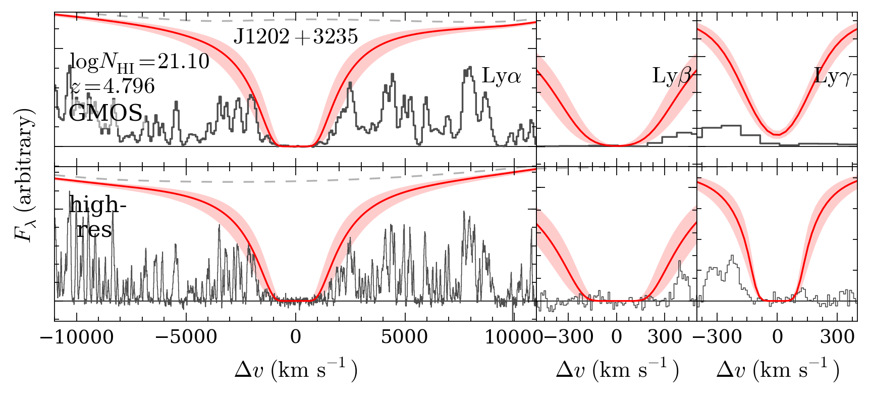
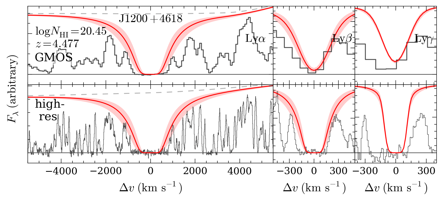
Two of the authors (NHMC and JXP) searched the spectra for DLAs independently. The above steps were done either using custom-written Python code, or with x_fitdla from xidl, depending on which author performed the search. For each QSO we also noted any properties of the spectrum which might complicate the identification of DLAs, such as the presence of broad absorption lines associated with the background QSO, or of possible problems with the sky background subtraction. Two example DLA candidates are shown in Figure 2. In these two cases, higher resolution spectra confirm that both candidates are indeed DLAs. The ${\it N}_{\mathrm{HI}}$ and redshift estimated from the GMOS spectra differ slightly from the values inferred from the higher resolution spectra – we discuss this issue further in Section 4.3. Once we assembled a list of DLA candidates, we selected only those within a redshift path limit defined by:

$$\begin{split}z_{\mathrm{min}}&=(1+z_{\mathrm{qso}})\frac{\lambda_{\mathrm{Ly\beta}}}{\lambda_{\mathrm{Ly\alpha}}}-1\\ z_{\mathrm{max}}&=(1+z_{\mathrm{qso}})(1-\delta v/c)-1\end{split}$$ (8)

where $\lambda_{\mathrm{Ly\alpha}}=1215.6701$ Å, $\lambda_{\mathrm{Ly\beta}}=1025.72$ Å and $\delta v=5000\,\rm km\,s^{-1}$. This $\delta v$ was chosen to exclude ‘proximate’ DLAs, whose incidence rate is likely affected by a combination of ionizing radiation from the background QSO, and by the overdensity associated with the QSO host galaxy halo (e.g. Ellison et al., 2002; Russell et al., 2006; Prochaska et al., 2008; Ellison et al., 2010). Table 5 lists the redshift path limits used for each QSO in the GGG sample. We then convert the redshift path for each QSO to an absorption distance path using equation (2).

Figure 2: DLAs identified in the GMOS spectra (resolution FWHM $\sim 230$ $\rm km\,s^{-1}$) which are confirmed in higher resolution ESI spectra (resolution FWHM $\sim 30$ $\rm km\,s^{-1}$). In each case the top panels show the GMOS spectrum and the bottom panels the ESI spectrum of the same QSO. The model shows the ${\it N}_{\mathrm{HI}}$ and redshift estimated from the ESI spectra with the redshift fixed by low-ion metal absorption. The shaded region shows an uncertainty in $\log{\it N}_{\mathrm{HI}}$ of 0.2. The ${\it N}_{\mathrm{HI}}$ and redshift estimated from the GMOS spectra are given in Table 4.

With these DLA candidate lists we can derive the measured incidence rate of DLAs, $f_{\mathrm{meas}}$. However, despite our attempt to take continuum uncertainties and IGM absorption into account when measuring ${\it N}_{\mathrm{HI}}$ for each DLA, large systematic uncertainties may remain. The following sections describe how we quantify these uncertainties using the correction factors $k_{\mathrm{real}}$ and $k_{\mathrm{found}}$ to $f_{\mathrm{meas}}$.

4.2 Estimation of $k_{\mathrm{real}}$ and $k_{\mathrm{found}}$

We expect $k_{\mathrm{real}}$ to be less than unity, meaning that there are some spurious DLA candidates. The rate of these spurious candidates is estimated in two ways. First, we use the sample of higher-resolution spectra to identify DLAs, and compare these with the DLA candidates found in the low-resolution sample. Second, we create mock low-resolution spectra which closely match the GMOS spectra and contain DLAs generated from a distribution at $z=3$, and then search these spectra for DLAs in the same way as the real spectra.

$k_{\mathrm{found}}$ is also expected to be less than unity, which means some true DLAs exist which we do not flag as DLA candidates in the low resolution spectra. Again we estimate the fraction of true DLAs recovered in two independent ways, using higher resolution spectra and mocks. In the first case DLAs identified in the higher resolution QSO spectra were used as a reference list of true DLAs, and compared to the candidate DLAs found in the lower resolution spectra of the same QSOs. In the second case we used mock GMOS spectra, which allow us to directly compare known DLAs in the spectra to the DLA candidates.

Our motivation for using two different ways to estimate the correction factors (mocks and high resolution spectra) is to test different systematic effects. The main advantage of the mocks is that the true DLA properties are known precisely. However, while we attempt to reproduce the real spectra as closely as possible, including $\rm Ly\alpha$ forest clustering, QSO redshift and signal-to-noise distribution, it is still possible that the mocks may differ from the real GMOS spectra. Metal absorption (not included in the mocks) or clustering of strong absorbers that is different to the mocks may cause more spurious DLAs. Alternatively, non-Gaussian noise in the real spectra at low fluxes may mean that true DLAs are more likely to be missed in the real spectra. Conversely, for the high-resolution sample the true DLA properties are not known with complete certainty, but the correct clustering, IGM blending, noise and metal absorption are all included. Therefore these two approaches provide complementary estimates of $k_{\mathrm{found}}$ and $k_{\mathrm{real}}$. The following sections describe these approaches in more detail.

4.2.1 Corrections using high resolution spectra

DLAs can be found more easily in our sample of high resolution spectra, and their ${\it N}_{\mathrm{HI}}$ and redshift are more accurately measured, in comparison to the lower resolution GMOS spectra. Therefore we independently identify DLAs in these spectra for the purpose of deriving the correction factors $k_{\mathrm{real}}$ and $k_{\mathrm{found}}$, and to test for any systematics in estimating ${\it N}_{\mathrm{HI}}$ and $z$ for each DLA. When identifying the DLAs in the 59 high-resolution spectra we follow the same process outlined for the lower-resolution spectra in Section 4.1, using the Lyman series to estimate the redshift and ${\it N}_{\mathrm{HI}}$. However, we also refine the redshift and ${\it N}_{\mathrm{HI}}$ using the position of low-ionization metal lines (O i, Si ii, C ii and Al ii) where possible. For the 20 QSOs with high-resolution spectra which are not in the GGG sample, we created low-resolution spectra by convolving the high-resolution spectra to the same FWHM resolution, and rebinning to the same pixel size as the GMOS spectra. The same noise array was used for these spectra as for the GGG QSO with a redshift closest to each QSO, normalising such that the median S/N within rest-frame wavelengths $1260$–$1280$ Å match. These low resolution spectra were searched for DLAs in the same way as the GMOS spectra.

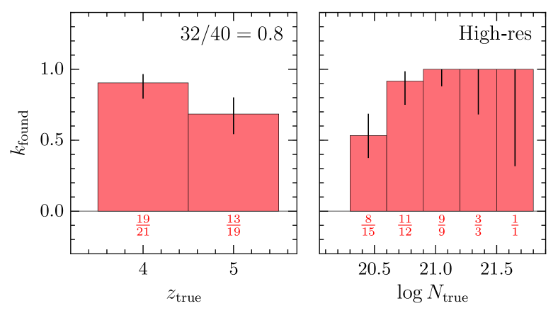
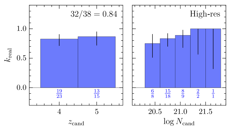
In this way we made two lists of DLAs, one from the high resolution spectra, and another from low-resolution spectra of the same QSOs. The DLAs identified in the higher resolution sample are listed in columns 5 and 6 of Table 4. We then estimated $k_{\mathrm{real}}$ as $N_{\mathrm{cand,true}}/N_{\mathrm{cand}}$, where $N_{\mathrm{cand}}$ is the number of DLA candidates from the low-resolution spectra, and $N_{\mathrm{cand,true}}$ is the number of those candidates confirmed to be DLAs by the high resolution spectra. $k_{\mathrm{found}}$ is estimated as $N_{\mathrm{cand,true}}/N_{\mathrm{true}}$, where $N_{\mathrm{true}}$ is the number of DLAs found in the high-resolution spectra and $N_{\mathrm{cand,true}}$ is the number of those also flagged as DLA candidates in the low resolution spectra. We calculate the binomial confidence intervals on $k_{\mathrm{real}}$ and $k_{\mathrm{found}}$ using the method described by Cameron (2011).

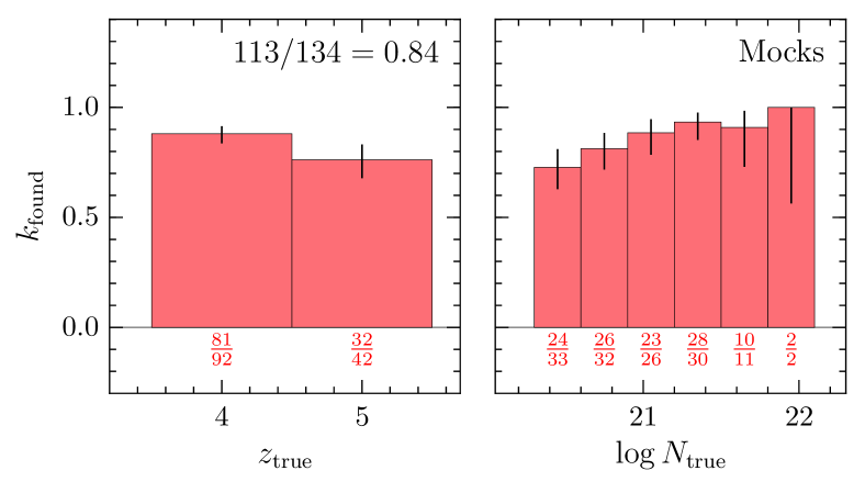
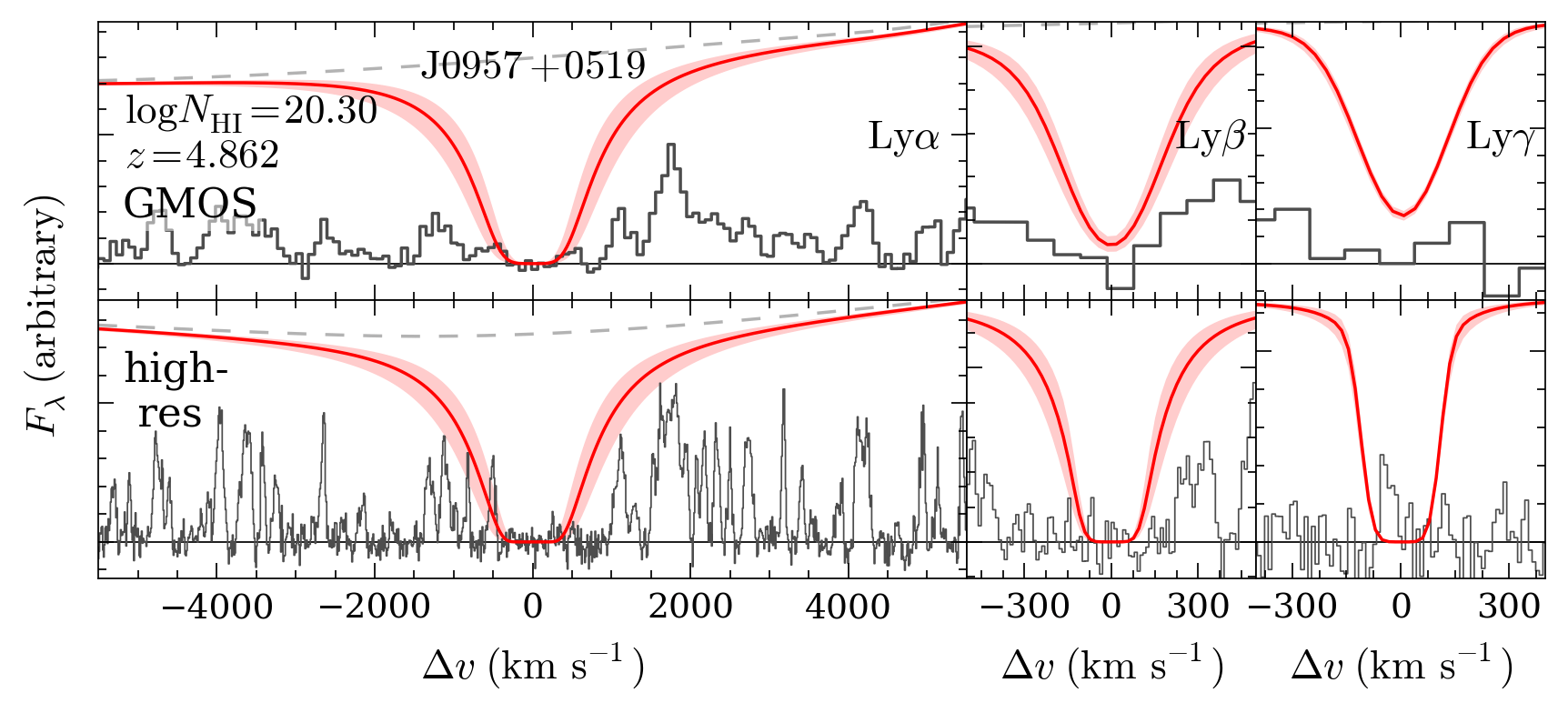
With this procedure we find $k_{\mathrm{real}}=0.80_{-0.08}^{+0.07}$ and $k_{\mathrm{found}}=0.84^{+0.06}_{-0.08}$ using DLAs identified by JXP (see Figures 5, 6) with similar values found by NHMC. Both are below unity, and so there are both spurious DLA candidates, and real DLAs missed. Spurious DLAs usually occur when flux spikes are smoothed away at GMOS resolution, making a lower ${\it N}_{\mathrm{HI}}$ system appear to have strong damping wings. An example spurious DLA is shown in Figure 3.

Figure 3: Example of a spurious DLA candidate. This was identified as a DLA with ${\it N}_{\mathrm{HI}}=10^{20.4\pm 0.2}$ cm^-2 in the GMOS spectrum shown in the top panels. However, the residual flux spikes at $\rm Ly\alpha$ and Ly$\gamma$ in the higher resolution (FWHM $\sim 30$ $\rm km\,s^{-1}$) ESI spectrum in the bottom panels show this system must have ${\it N}_{\mathrm{HI}}<10^{20.3}$ cm^-2.

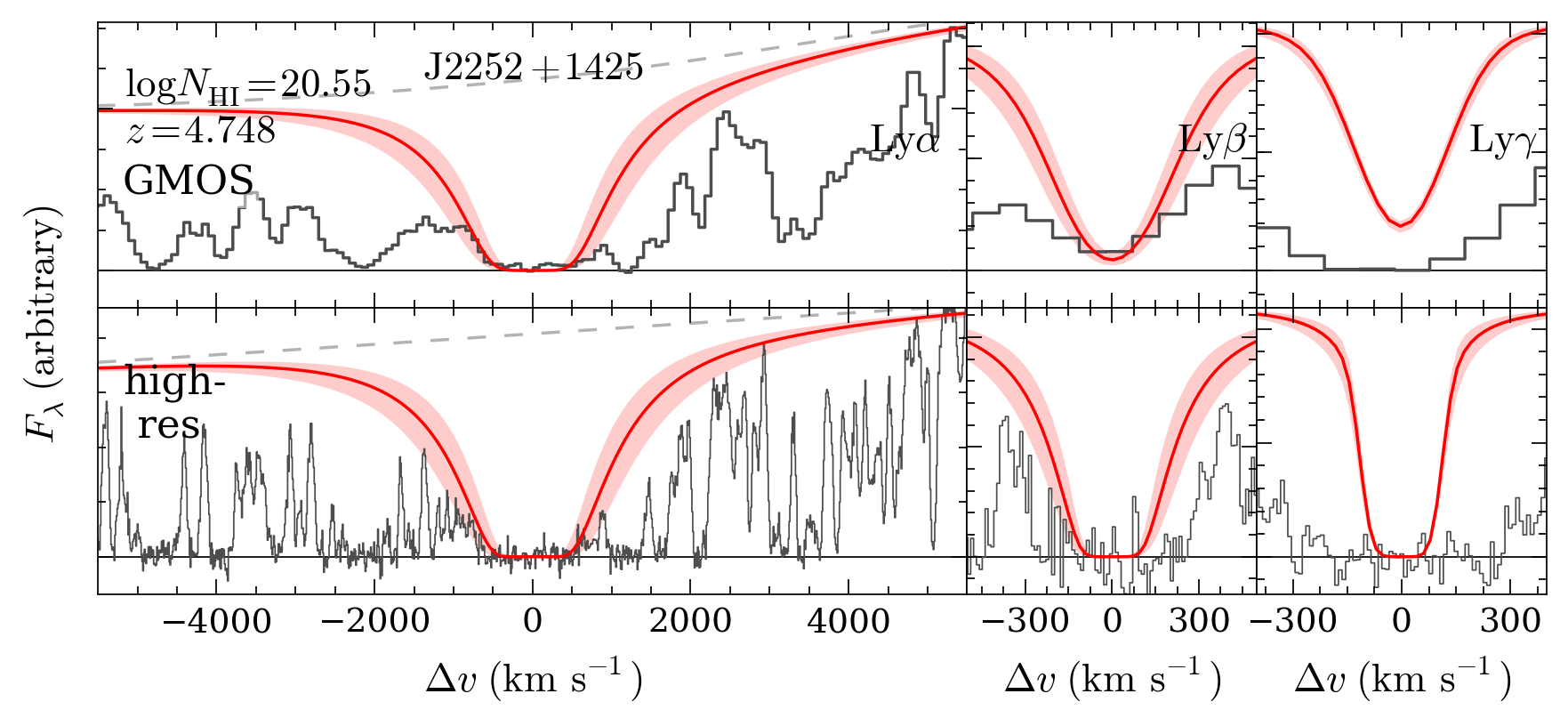
Real DLAs are generally missed due to flux fluctuations in the core of the $\rm Ly\alpha$ line: an example is shown in Figure 4.

Figure 4: A DLA that was not correctly identified in the GMOS spectra. Lower panels show the DLA in the ESI spectrum, with ${\it N}_{\mathrm{HI}}=10^{20.55\pm 0.2}$ cm^-2. The residual flux in the core of the $\rm Ly\alpha$ line in the GMOS spectrum, however (top left panel), meant this system was missed. This residual flux around velocities $\Delta v\sim 0$ $\rm km\,s^{-1}$ may be caused by either statistical fluctuations or systematics associated with sky background level.

4.2.2 Corrections using mock spectra

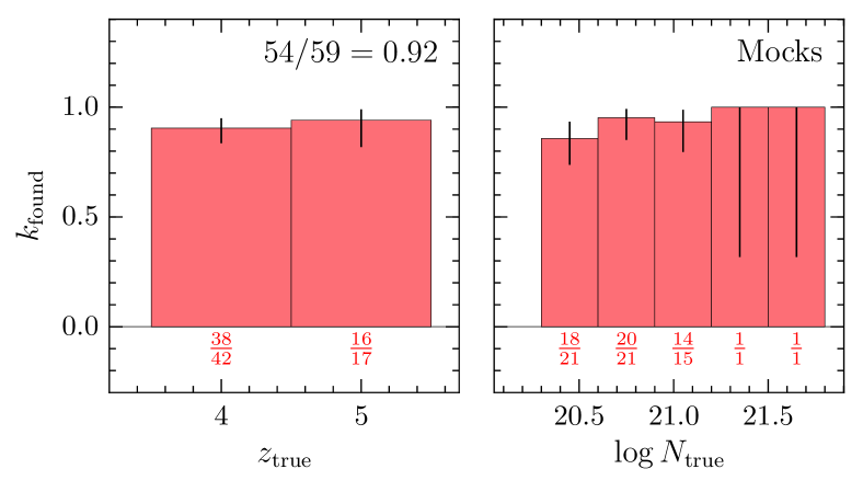
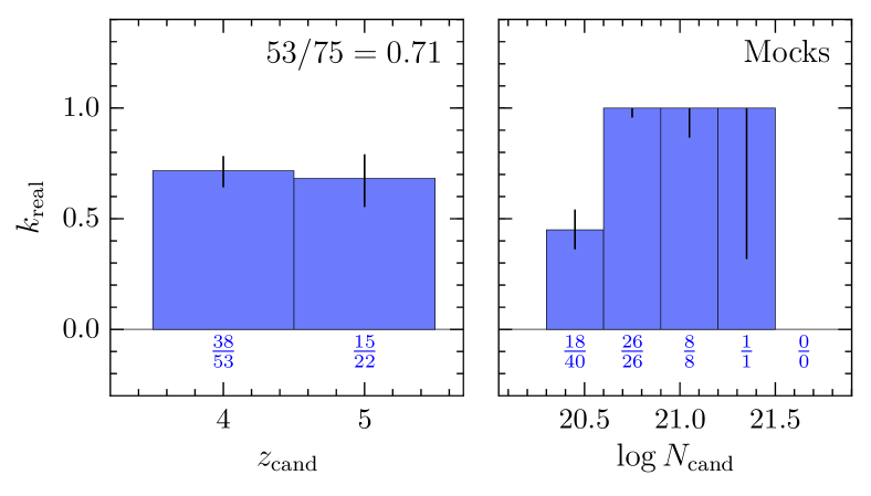
Our method for generating mock spectra is described in Appendix A. In this case the ${\it N}_{\mathrm{HI}}$ for each DLA is known, and so can be directly compared to the candidates identified in the low-resolution mocks. Again $k_{\mathrm{real}}$ is estimated as $N_{\mathrm{cand,true}}/N_{\mathrm{cand}}$, where $N_{\mathrm{cand}}$ is the number of DLA candidates from the low-resolution mock spectra, and $N_{\mathrm{cand,true}}$ is the number of those candidates that are DLAs. $k_{\mathrm{found}}$ is estimated as $N_{\mathrm{cand,true}}/N_{\mathrm{true}}$, where $N_{\mathrm{true}}$ is the true number of DLAs in the mocks and $N_{\mathrm{cand,true}}$ is the number of those recovered as DLA candidates. Again we calculate the errors on $k_{\mathrm{real}}$ and $k_{\mathrm{found}}$ assuming a binomial confidence interval. For the mocks we find $k_{\mathrm{real}}=0.71\pm 0.06$ and $k_{\mathrm{found}}=0.92^{+0.04}_{-0.07}$ using DLAs identified by JXP (see Figures 5, 6). Similar values are found by NHMC (see Figures 16, 17).

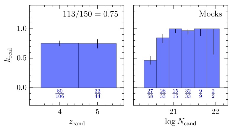
4.2.3 Comparison of correction factors and their dependence on redshift and column density

We expect $k_{\mathrm{real}}$ and $k_{\mathrm{found}}$ to be a function of a DLA’s ${\it N}_{\mathrm{HI}}$ (high ${\it N}_{\mathrm{HI}}$ candidates should be more reliable), spectral S/N (low S/N spectra will produce more spurious candidates) and redshift (more spurious DLAs will be found at high redshift where there is more IGM absorption). The most important of these for our measurement of $\rm\Omega_{\rm HI}$ is any redshift or ${\it N}_{\mathrm{HI}}$ dependence. Noterdaeme et al. (2009) and Noterdaeme et al. (2012) show that at $z\sim 2.5$, systems with ${\it N}_{\mathrm{HI}}=10^{20.6-21.5}~{}\rm cm^{-2}$ make the largest contribution to $\rm\Omega_{\rm HI}$. Thus we expect completeness corrections in this column density range to have the largest effect on the final derived $\rm\Omega_{\rm HI}$.

The top panels of Figure 5 show the correction factor $k_{\mathrm{found}}$ from the high-resolution spectra binned by the true DLA redshift and ${\it N}_{\mathrm{HI}}$, and the bottom panels show the same correction factor estimated from the mocks. Figure 6 shows the correction factor $k_{\mathrm{real}}$ binned by the candidate DLA redshift and ${\it N}_{\mathrm{HI}}$, again for the high-resolution spectra and mocks. These are derived from DLAs identified by one of the authors (JXP) who search the spectra for DLAs, but values for the other author (NHMC) are similar. There is no evidence for a strong dependence of $k_{\mathrm{real}}$ or $k_{\mathrm{found}}$ on redshift, using either the high-resolution spectra or the mocks. However, there is a weak dependence of $k_{\mathrm{real}}$ and $k_{\mathrm{found}}$ on ${\it N}_{\mathrm{HI}}$, with the lowest ${\it N}_{\mathrm{HI}}$ bin having a significantly lower $k_{\mathrm{real}}$ than for higher ${\it N}_{\mathrm{HI}}$ bins. This matches our expectations: weaker candidate DLAs are more likely to be spurious, and true DLAs that are weak are more likely to be missed. We take this ${\it N}_{\mathrm{HI}}$ dependence into account when applying the correction factors as described in Section 5. We find no strong dependence of the correction factors on S/N in either the mocks or the high-resolution sample for the range of S/N the GMOS spectra cover.

Figures 5 and 6 also show that corrections derived from the mocks and high-resolution spectra are in reasonable agreement. The main difference is in the number of spurious systems with ${\it N}_{\mathrm{HI}}\sim 10^{20.3-20.6}$ cm^-2. The right hand panels of Figure 6 show that there are more weak, spurious DLAs found in the mocks compared to the real GMOS spectra. However, we show in the following section that the correction factor in this ${\it N}_{\mathrm{HI}}$ range is not important for estimating $\rm\Omega_{\rm HI}$, and for the remaining bins the mocks and high-resolution corrections match to within $20$ per cent. As we discussed earlier, the high-resolution sample and mocks test different systematic uncertainties which may affect $\rm\Omega_{\rm HI}$. Therefore the consistency of the correction factors between these two methods suggests the mocks reproduce the true GMOS spectra well, and that DLAs have been identified correctly in the higher-resolution spectra.

Figure 5: The fraction of true DLAs that were correctly identified by one of the authors (JXP), $k_{\mathrm{found}}$, as a function of the true redshift and ${\it N}_{\mathrm{HI}}$. Top panels are for the high-resolution sample, bottom panels are for mocks. The upper row of numbers under each histogram gives the number of DLA candidates that are correct per bin, the lower row the total number of candidates. The total numbers for all bins are given at the top in the left panels. Vertical lines show the binomial $68\%$ uncertainties.

Figure 6: The fraction of non-spurious DLA candidates, $k_{\mathrm{real}}$ by one of the authors (JXP), as a function of the candidate redshift and ${\it N}_{\mathrm{HI}}$. Top panels are for the high-resolution sample, bottom panels are for mocks. The upper row of numbers under each histogram gives the number of true DLAs that are recovered per bin, the lower row the total number of true DLAs. The total numbers for all bins are given at the top of the left panels. Vertical lines show the binomial $68\%$ uncertainties.

4.3 Uncertainties in ${\it N}_{\mathrm{HI}}$ and redshift

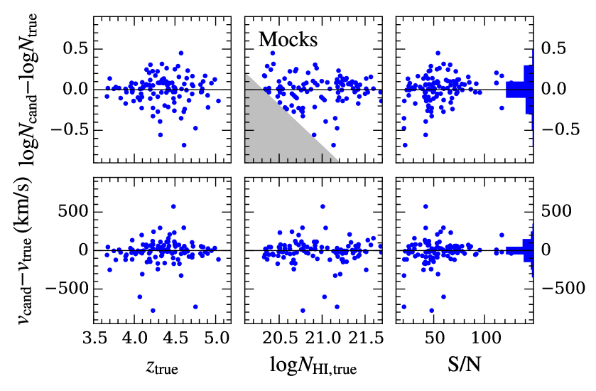
If DLA column densities estimated from the GMOS spectra are systematically in error, our measurement of $\rm\Omega_{\rm HI}$ may be biased. Such a systematic could occur because of incorrect placement of the continuum, or blending of damping wings with the $\rm Ly\alpha$ forest. This is an additional effect not accounted for by the correction factor, $k$, to $f_{\mathrm{meas}}$. Therefore, we search for any systematic offset in ${\it N}_{\mathrm{HI}}$ by matching DLA candidates from the low-resolution spectra to known DLAs in the high-resolution sample and mocks.

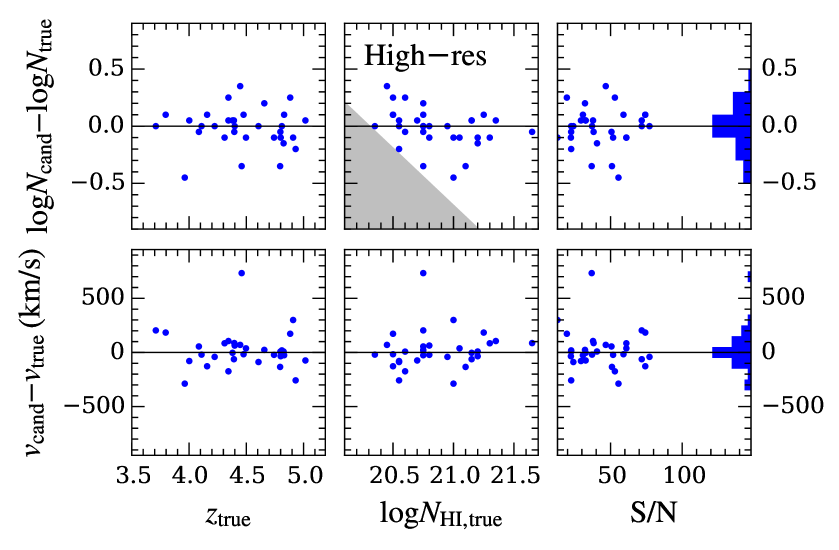
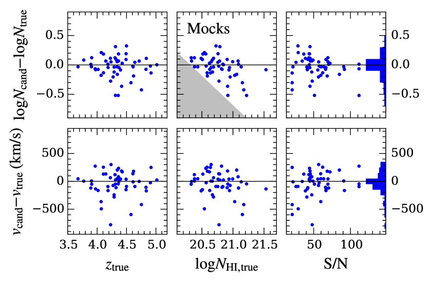
The results of this test are shown in Figure 7. The log ${\it N}_{\mathrm{HI}}$ difference is plotted as a function of redshift, the true ${\it N}_{\mathrm{HI}}$, and S/N for the high-resolution sample (top panels) and mocks (bottom panels). For both the mocks and high-resolution samples, both $\Delta\log{\it N}_{\mathrm{HI}}$ and $\Delta v$ are centred on 0. The standard deviation of the velocity and $\log{\it N}_{\mathrm{HI}}$ offsets are 184/216 $\rm km\,s^{-1}$ and 0.165/0.196 for the high-resolution sample and mocks, respectively. We therefore adopt 0.2 dex as our uncertainty in ${\it N}_{\mathrm{HI}}$. There is no trend seen with redshift or S/N. There may be a trend with ${\it N}_{\mathrm{HI}}$, but above $N=10^{20.3}~{}\rm cm^{-2}$ it is too weak to significantly affect $\rm\Omega_{\rm HI}$. We conclude that there is no systematic bias in ${\it N}_{\mathrm{HI}}$ which might adversely affect the $\rm\Omega_{\rm HI}$ measurement.

Figure 7 also shows the redshift difference between matched DLAs expressed as a velocity difference. DLAs identified in the higher resolution spectra use low-ionization metal lines to set a precise DLA redshift with an error a few $\rm km\,s^{-1}$. Both the mocks and high resolution sample show that an uncertainty of $\sim 200$ $\rm km\,s^{-1}$ results from estimating redshifts using Lyman series absorption alone (without reference to metal absorption) in the low-resolution spectra.

Figure 7: The difference between ${\it N}_{\mathrm{HI}}$ estimated for DLA candidates in low resolution spectra ($N_{\mathrm{HI,cand}}$) and $N_{\mathrm{HI,true}}$ measured from high resolution spectra (top) or known from mock linelists (bottom), and similarly for the velocity offset from the true DLA redshift. This is for one of the authors (JXP), but the results for NHMC are similar. These show there is no strong systematic offset in the estimated ${\it N}_{\mathrm{HI}}$ as a function of redshift, S/N or ${\it N}_{\mathrm{HI}}$ which might systematically bias $\rm\Omega_{\rm HI}$ significantly. Grey shading shows regions that cannot be populated due to the requirement that both $N_{\mathrm{HI,cand}}$ and $N_{\mathrm{HI,true}}$ are $>10^{20.3}$ cm^-2.

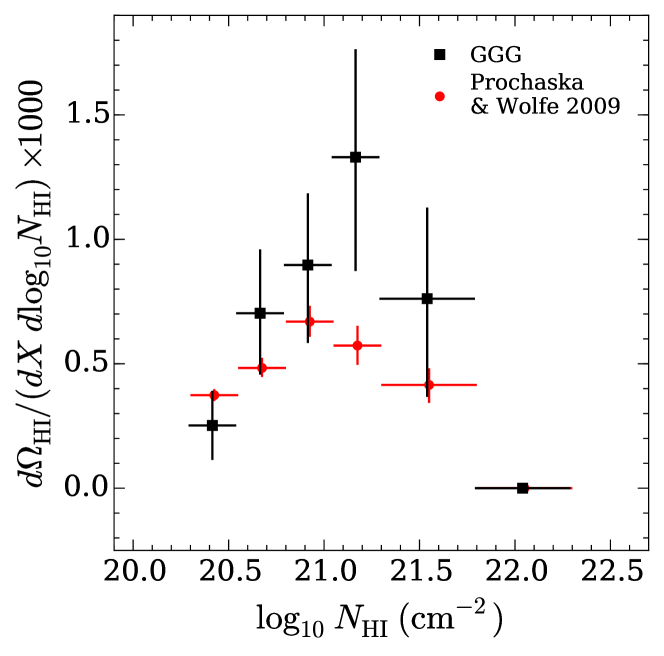
4.4 DLA incidence rate and differential ${\it N}_{\mathrm{HI}}$ distribution

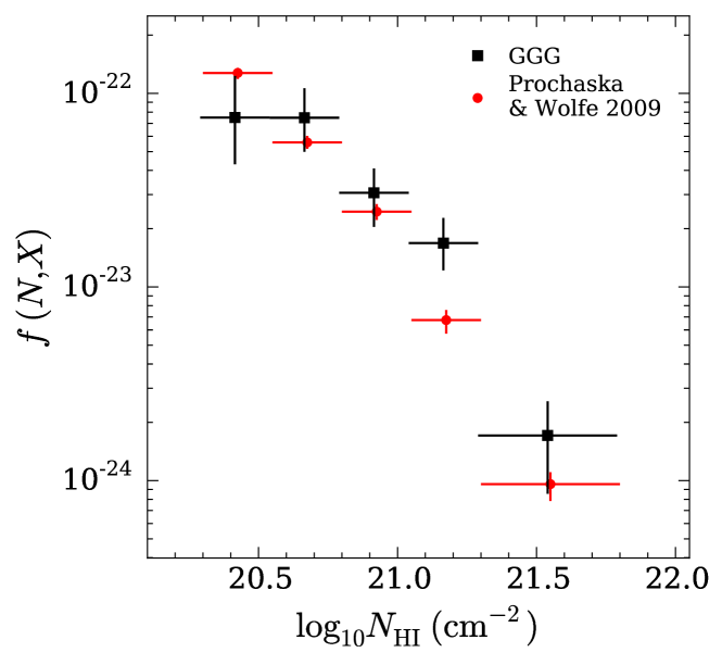
Figure 8 shows the differential ${\it N}_{\mathrm{HI}}$ distribution from the GGG sample compared to that from the SDSS sample from Prochaska & Wolfe (2009), which is consistent with the more recent estimate from Noterdaeme et al. 2012. We have four different measurements of the correction factor $k({\it N}_{\mathrm{HI}})$, from two different authors using the mocks and high-resolution spectra, so there are four different estimates of $f({\it N}_{\mathrm{HI}},X)$. We find the final $f({\it N}_{\mathrm{HI}},X)$ by averaging these four estimates. The uncertainties on this value include a statistical and systematic component. The statistical uncertainty is found by bootstrap resampling, using 1000 samples from the observed DLA distribution, and averaging these uncertainties for the four different estimates. The systematic uncertainty is then assumed to be the standard deviation in the four estimates. These systematic and statistical components are added in quadrature to give the errors shown in figure 8. The two distributions are similar overall, although there is a clear discrepancy between the GGG and $z=3$ $f({\it N}_{\mathrm{HI}},X)$ for the bin at $\log{\it N}_{\mathrm{HI}}\sim 21.2$, which hints at evolution in the shape of $f({\it N}_{\mathrm{HI}},X)$ at high redshift. However, a simple change in the normalization is also consistent with the data.

The DLA incidence rate, $\ell(X)$, is shown in Figure 9. This observable is more sensitive to the lowest ${\it N}_{\mathrm{HI}}$ DLAs than $\rm\Omega_{\rm HI}$. Since the correction factors we derive are strongest for low ${\it N}_{\mathrm{HI}}$ DLAs and these DLAs have a strong effect on $\ell(X)$, we expect $\ell(X)$ to be sensitive to the particular choices of correction factors. This is indeed the case – there are systematic differences at least as large as the statistical errors, and they depend on whether the mocks or the high resolution spectra are used to estimate the correction factor. Similarly large differences are found between $\ell(X)$ by each of the two authors who searched for DLAs. The $\ell(X)$ values we measure are consistent with a smooth increase from $z=2$ to $z=5$. However, since we do not know which $k({\it N}_{\mathrm{HI}})$ correction factors are best, we do not attempt to present a definitive $\ell(X)$ measurement here. A large sample of higher-resolution spectra, where low column density DLAs can be identified with more certainty, will be necessary to robustly measure $\ell(X)$ at $z>4$.

We can still make a more robust measurement of $\rm\Omega_{\rm HI}$, however, regardless of the uncertainty in $\ell(X)$, as Figure 10 illustrates. DLAs with the largest contribution to $\rm\Omega_{\rm HI}$ have ${\it N}_{\mathrm{HI}}$ in the range $10^{20.8}$–$10^{21.6}$ cm^-2, and DLAs with lower ${\it N}_{\mathrm{HI}}$ make a substantially smaller contribution. Therefore, while systematic effects may give rise to a large uncertainty in the number of low column density systems (and thus $\ell(X)$), $\rm\Omega_{\rm HI}$ can still be measured accurately. This point is discussed further in Section 5.

Figure 8: The column density distribution, $f({\it N}_{\mathrm{HI}})$, for the GGG sample of DLAs. Black points show the measurements with correction $k({\it N}_{\mathrm{HI}})$ applied. Both are slightly offset in ${\it N}_{\mathrm{HI}}$ for clarity. Red points show the SDSS DR5 measurements from Prochaska & Wolfe (2009) after applying the correction to the redshift search path recommended by Noterdaeme et al. (2009). The errors are $1\sigma$, and include statistical and systematic errors (see section 4.4 for more details).

Figure 9: The DLA incidence rate $\ell(X)$. This observable is more sensitive to the lowest ${\it N}_{\mathrm{HI}}$ DLAs than $\rm\Omega_{\rm HI}$. Grey points show the uncorrected GGG measurement, and black squares with the corrections applied. Each panel shows a different correction, using either mock or high-resolution spectra for two different authors. There are systematic differences comparable to the statistical errors, and they depend on whether the mocks or the high resolution spectra are used to estimate correction factors. Similar differences are also found between the two different authors who searched for DLAs. These illustrate that significant systematic uncertainties affect the measurement of $\ell(X)$.

Figure 10: The differential $\rm\Omega_{\rm HI}$ distribution, $d\rm\Omega_{\rm HI}/(dXd\log{\it N}_{\mathrm{HI}})$. DLAs with the largest contribution to $\rm\Omega_{\rm HI}$ have ${\it N}_{\mathrm{HI}}$ in the range $10^{20.8}$–$10^{21.6}$ cm^-2; DLAs with lower ${\it N}_{\mathrm{HI}}$ are less important. Therefore, while there is uncertainty in the number of low column density systems (and thus $\ell(X)$), $\rm\Omega_{\rm HI}$ can still be measured accurately. This is also illustrated by Figure 11.

5 Results and discussion

5.1 $\rm\Omega_{\rm HI}$ measurement

We can now use the ${\it N}_{\mathrm{HI}}$-dependent correction factor $k$ estimated in the previous section to find $f_{\mathrm{DLA}}$ and thus $\rm\Omega_{\rm HI}$. For the GGG sample we count the number of DLAs in a given absorption path, giving each DLA a weight $k({\it N}_{\mathrm{HI}})$, where $k({\it N}_{\mathrm{HI}})=k_{\mathrm{found}}({\it N}_{\mathrm{HI}})/k_{\mathrm{real}}({\it N}_{\mathrm{HI}})$. $k({\it N}_{\mathrm{HI}})$ is then estimated as the ratio of the $\log{\it N}_{\mathrm{HI}}$ histograms shown in Figures 5 and 6, with the uncertainty on each bin given by the uncertainties in $k_{\mathrm{found}}$ and $k_{\mathrm{real}}$ added in quadrature.

There are two main contributions to the final error on $\rm\Omega_{\rm HI}$. The dominant contribution is the statistical error due to the finite sampling of DLAs: there are $25$–$30$ DLA candidates in each redshift bin, dependent on whether NHMC or JXP’s results are used. We estimate this error using 1000 bootstrap samples from the DLA sample. The second is the systematic uncertainty in the correction factor, $k({\it N}_{\mathrm{HI}})$. We estimate the effect of this uncertainty using a Monte Carlo technique. $\rm\Omega_{\rm HI}$ is calculated 1000 times, each time drawing $k({\it N}_{\mathrm{HI}})$ from a normal distribution with a mean given by the $k({\it N}_{\mathrm{HI}})$ histogram bin value and $\sigma$ determined by the uncertainty on that bin, assuming no correlation between uncertainties in adjacent bins. Then the final error in $\rm\Omega_{\rm HI}$ is given by adding these two uncertainties in quadrature. We confirmed that ${\it N}_{\mathrm{HI}}$ error of each DLA (0.2 dex, see Section 4.3), has a negligible contribution compared to these statistical and systematic uncertainties. We also check that using ${\it N}_{\mathrm{HI}}$ measurements from the high-resolution spectra, where available, does not significantly change $\rm\Omega_{\rm HI}$.

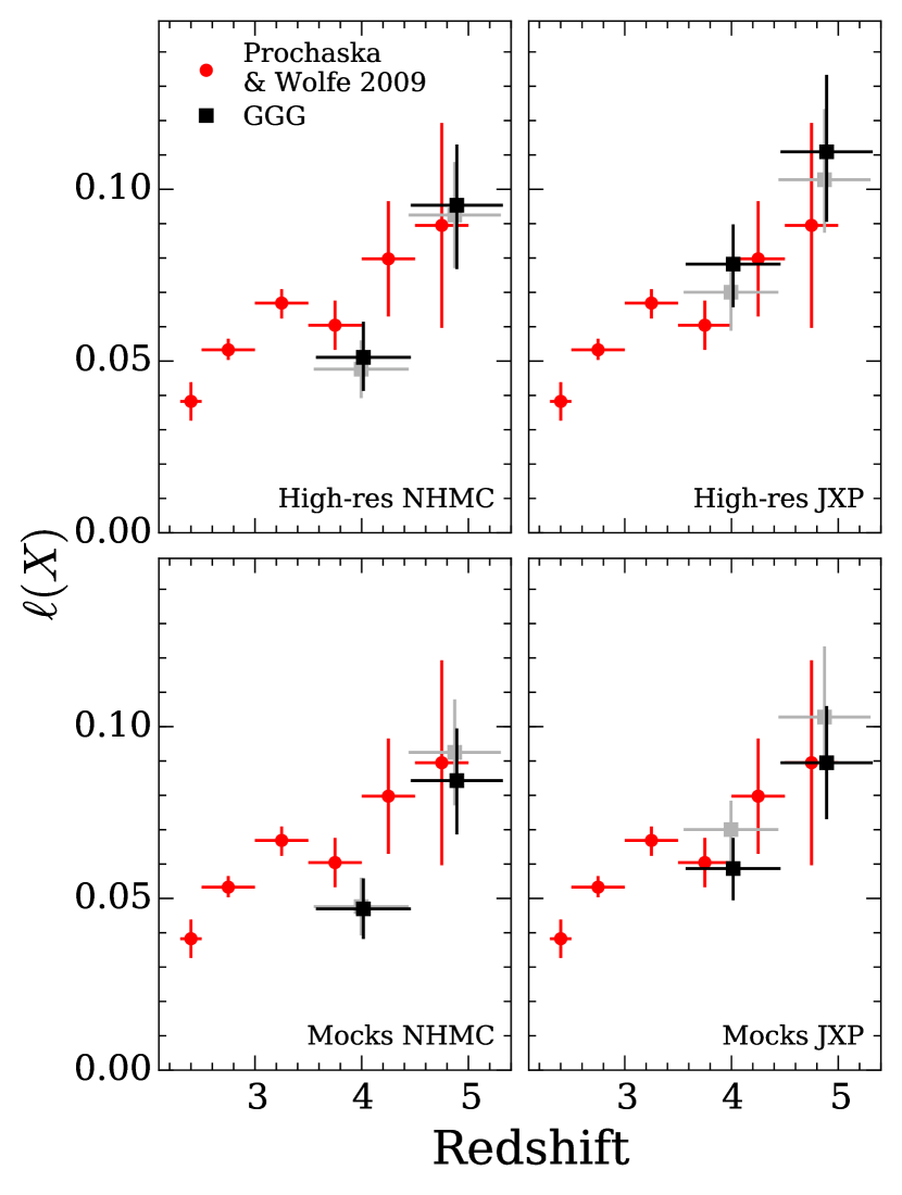
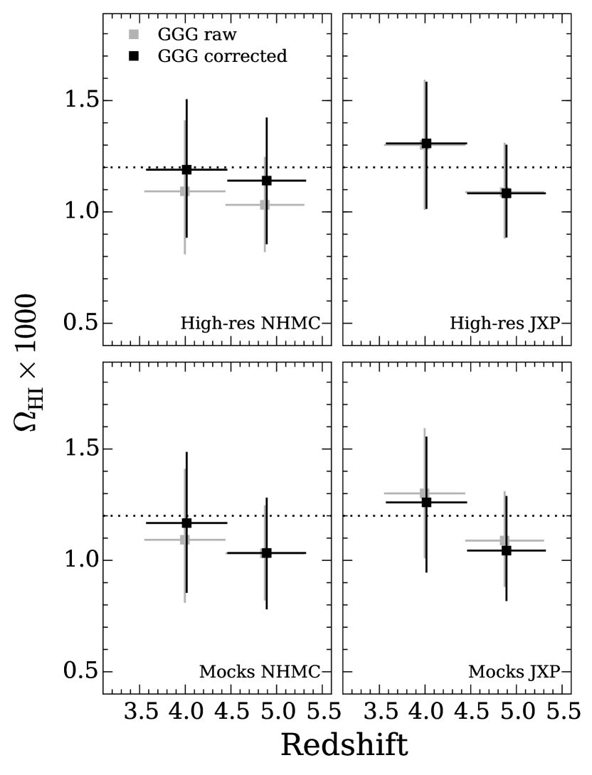
Since we have separate estimates of $k({\it N}_{\mathrm{HI}})$ from the mocks and high resolution sample, and two authors performed these estimates, we can make 4 different measurements of $\rm\Omega_{\rm HI}$. We use these to gauge the effect on $\rm\Omega_{\rm HI}$ of estimating corrections from the mocks versus the high-resolution sample, or of any differences in the way the two authors identified DLAs. The results are shown in Figure 11. The differences between the mocks compared to the high-resolution sample, and between the two authors, are significantly smaller than the uncertainty on any individual $\rm\Omega_{\rm HI}$ measurement. Therefore we conclude that neither the methods we use to estimate $k({\it N}_{\mathrm{HI}})$, nor any differences in DLA detection between methods, contribute a significant uncertainty to the final $\rm\Omega_{\rm HI}$. We caution that this conclusion only holds for the sample of spectra we analyse. New tests of systematic effects may be required for measurements of $\rm\Omega_{\rm HI}$ using larger samples of DLAs, or using different resolution or S/N QSO spectra.

For the remainder of the paper we use the measurement of $\rm\Omega_{\rm HI}$ derived using $k$ from the higher-resolution sample and measured by author JXP, which is shown in the top-right panel of Figure 11. This measurement and the 68% confidence interval is given in Table 1. We assume a 20% contribution to $\rm\Omega_{\rm HI}$ from systems below the DLA threshold, as described in Section3.2.

Figure 11: $\rm\Omega_{\rm HI}$ measured by the two authors using the high-resolution sample (top) and mocks (bottom). The uncertainties on $\rm\Omega_{\rm HI}$ introduced by any differences in selecting DLA candidates between the authors, or between using mocks or the high-resolution sample, are much smaller than the errors shown, which are a combination of the statistical error and uncertainty in the correction factor (see section 5).

$z$	$10^{3}\,\rm\Omega_{\rm HI}$	$10^{3}\,\rm\Omega_{\rm HI}$ $(1\sigma)$	$\Delta X$
3.56-4.45	1.18	0.92-1.44	356.9
4.45-5.31	0.98	0.80-1.18	194.6

Table 1: $\rm\Omega_{\rm HI}$ for the GGG sample, assuming a flat cosmology with $H_{0}=70$ $\rm km\,s^{-1}\,Mpc^{-1}$ and $\Omega_{m,0}=0.3$. The redshift bins were chosen to cover roughly equal redshift widths, and to yield approximately equal numbers of DLAs in each bin. To convert between $\rm\Omega_{\rm HI}$ and $\rm\Omega^{\rm DLA}_{g}$, which is often quoted by other DLA studies, use $\rm\Omega_{\rm HI}=\delta_{\rm HI}\rm\Omega^{\rm DLA}_{g}/\mu$, where $\mu=1.3$ accounts for the mass of helium and $\delta_{\rm HI}=1.2$ estimates the contribution from systems below the DLA threshold of $10^{20.3}$ cm^-2.

5.1.1 Is there a bias from gravitational lensing?

There is a $30\pm 20$% increase in $\rm\Omega_{\rm HI}$ for sightlines towards the brighter half of our QSO sample ($z\leq 19.2$ mag) relative to $\rm\Omega_{\rm HI}$ towards the fainter QSOs ($z>19.2$ mag). If this effect is caused by gravitational lensing of a background QSO by a galaxy associated with a foreground DLA, then our measured $\rm\Omega_{\rm HI}$ will be artificially enhanced. A detailed lensing analysis is beyond the scope of this work. However, if we follow Ménard & Fukugita (2012) and assume the lensing DLA galaxies are isothermal spheres, we can estimate their Einstein radius as

$$\zeta_{0}=4\pi\left(\frac{\sigma_{v}}{c}\right)^{2}\frac{D_{l}D_{ls}}{D_{s}}$$ (9)

where $\sigma_{v}$ is the velocity dispersion, $c$ is the speed of light and $D_{l,s,ls}$ are the angular diameter distances from the observer to the lens and to the source, and from the lens to the source. Assuming a typical dispersion of $100$ $\rm km\,s^{-1}$ we find the effective radius for lensing is very small, $0.1$ kpc for a $z=4.5$ DLA towards a $z=5$ QSO. This is half the radius for a DLA at $z=2.5$ towards a QSO at $z=3.5$. Since the magnitude of the increase in $\rm\Omega_{\rm HI}$ due to the putative lensing at $z\sim 3$ is relatively small ($\sim 20\pm 10$ per cent, Prochaska et al. 2005) we do not expect it to have a large effect at higher redshifts. We conclude that it is more likely the difference in $\rm\Omega_{\rm HI}$ between the bright and faint QSO samples is caused by a statistical fluctuation, rather than a lensing bias.

5.2 Comparison with previous measurements

Several groups have made measurements of $\rm\Omega_{\rm HI}$ at $z>4.5$ using DLA surveys (Péroux et al. 2003, Guimarães et al. 2009, S10). These are cumulative results – $\rm\Omega_{\rm HI}$ measurements from each new QSO sample are combined with older $\rm\Omega_{\rm HI}$ measurements which used a different DLA survey. While combining results in this way maximizes the statistical S/N of the final result, it results in a heterogeneous sample of quasar spectra with different data quality and different DLA identification methods. As shown in sections 4 and 5.1, at $z>4.4$ different identification methods can produce a systematic uncertainty in $\rm\Omega_{\rm HI}$ which, although smaller than the statistical uncertainties for our current DLA sample, may still be considerable. Since these analyses did not use mock spectra to explore systematic effects, it is difficult to estimate the true uncertainty in $\rm\Omega_{\rm HI}$ when combining heterogeneous quasar samples with different selection criteria. In contrast, our sample has homogeneous data quality, QSO selection method and DLA identification procedure, and we use mock spectra to test any systematic effects.

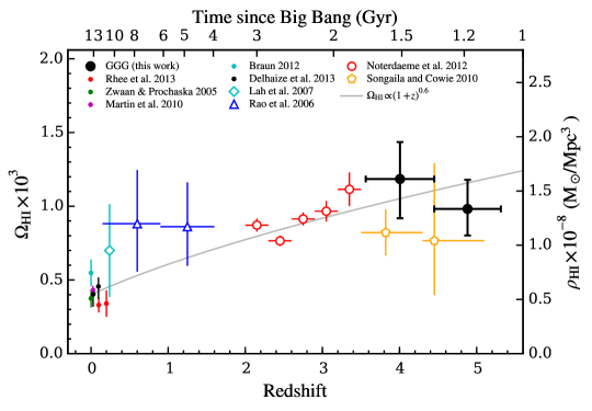
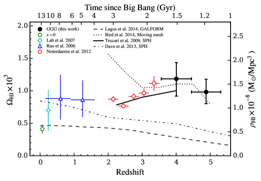
Figure 12 shows our new results together with previous measurements of $\rm\Omega_{\rm HI}$, converted to our adopted cosmology. When multiple measurements of $\rm\Omega_{\rm HI}$ have been made using overlapping QSO samples and the most recent measurement uses a superset of previous QSO samples, only the most recent measurement is shown. For example, the results of S10 include most of the quasars used by Péroux et al. (2003) and Guimarães et al. (2009), so we show only the S10 result. In all such cases the most recent measurement is consistent with earlier results. Where previous DLA surveys have quoted $\rm\Omega^{\rm DLA}_{\rm HI}$, we convert to $\rm\Omega_{\rm HI}$ using the relationship $\rm\Omega_{\rm HI}=1.2\rm\Omega^{\rm DLA}_{\rm HI}/1.3$. Our measurement at $\langle z\rangle=4$ is higher than, but consistent with earlier measurements by S10. As such and because we find a possible systematic increase in $\rm\Omega_{\rm HI}$ towards bright QSOs, we checked whether the magnitude distribution of the S10 QSOs was lower than the GGG sample. $z$ band data was not available for the whole S10 sample, but the eight QSOs which overlap between their sample and ours have a similar fraction of QSOs with $z\leq 19.2$ and $z>19.2$ mag. Therefore a difference in QSO magnitudes is unlikely to cause a difference between our result and the S10 result, and it seems more likely that the difference is caused by a statistical fluctuation.

Our results at $\langle z\rangle=4.9$ give the most robust indication to date that there is no strong evolution in $\rm\Omega_{\rm HI}$ over the $\sim 1$ Gyr period from $z=5$ to $z=3$. We see a slight drop in $\rm\Omega_{\rm HI}$ between our $z\sim 4$ and $z\sim 4.9$ $\rm\Omega_{\rm HI}$ measurements, but this difference is not statistically significant. If the metal content of DLAs does change suddenly at $z=4.7$, as suggested by Rafelski et al. (2014), there is no evidence it is accompanied by a concomitant change in $\rm\Omega_{\rm HI}$. However, the uncertainties remain large and future observations should continue to test this possibility.

Figure 12 also shows a power law with the form $\Omega_{\rm HI}=A(1+z)^{\gamma}$ fitted to the binned data. This simple function provides a reasonable fit ($\chi^{2}$ per degree of freedom $=1.44$) across the full redshift range, with best-fitting parameters $A=(4.00\pm 0.24)\times 10^{-4}$ and $\gamma=0.60\pm 0.05$. There is no obvious physical motivation for this relation, nor any expectation that it should apply at redshifts $>5$. Nevertheless, it may provide a useful fiducial model to compare to simulations and future observations.

Figure 12: Measurements of $\rm\Omega_{\rm HI}$ at different redshift, from Zwaan et al. (2005); Rao et al. (2006); Lah et al. (2007); Braun (2012); Martin et al. (2010); Noterdaeme et al. (2012); Rhee et al. (2013); Delhaize et al. (2013) and S10 (see Table 2). We do not show the measurement using SDSS QSOs by Prochaska & Wolfe (2009), it is consistent with the measurement by Noterdaeme et al. (2012), who use a superset of SDSS QSOs. We also do not show the Péroux et al. (2003) and Guimarães et al. (2009) results, which have a large overlap with the QSO sample used by S10 and are consistent with that measurement. Finally, for clarity we do not show the measurements at lower redshift from Freudling et al. (2011) and Meiring et al. (2011); they are consistent with the plotted values. All measurements have been converted to the same cosmology ($h=0.7$, $\Omega_{m}=0.3$, $\Omega_{\Lambda}=0.7$) and include H i mass only, with no contribution from helium or molecular hydrogen.

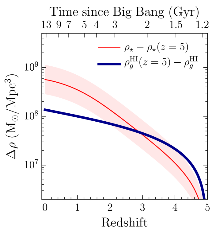
We also compare our new high-redshift value to lower redshift $\rm\Omega_{\rm HI}$ measurements. As previous authors have noted (e.g. Prochaska et al., 2005; Prochaska & Wolfe, 2009; Noterdaeme et al., 2009), $\rm\Omega_{\rm HI}$ evolves from $z=3$ to $z=0$ by factor of $\lesssim 2$, at odds with the very strong evolution in the star formation rate over the same period. Moreover, the drop in $\rm\Omega_{\rm HI}$ is much smaller than the increase in stellar mass over this period. Figure 13 demonstrates this point by showing the increase in comoving mass density in stars from $z=5$, $\rho_{\star}-\rho_{\star}(z=5)$ and the contemporaneous decrease in H i comoving gas mass density, $\rho^{\mathrm{HI}}_{g}(z=5)-\rho^{\mathrm{HI}}_{g}$ using the power law fit from Figure 12. The mass in stars is calculated using the expression from Madau & Dickinson (2014), and the range shows an uncertainty of $50\%$, indicative of the scatter in observations around this curve. While the evolution of $\rm\Omega_{\rm HI}$ from $z=5$ to $z=3$ remains uncertain, the H i phase at $z=5$ contains ample mass density to form all the stars observed at $z\sim 3$, and the evolution predicted by the simple power law function is consistent with this scenario. From $z\sim 3$ to $z\sim 0$, however, there is a factor of $5$–$6$ shortfall in H i mass density compared to amount needed to produce stars over the same period. This underscores that at $z\lesssim 3$, the H i phase must be continually replenished by more highly ionized gas, presumably through a combination of cold-mode accretion (e.g. Dekel et al., 2009) and recycled winds (e.g. Oppenheimer et al., 2010). The more highly ionized Lyman limit systems and sub-DLAs should then be important tracers of the interface between this H i phase and more highly ionized gas (e.g. Fumagalli et al., 2011).

Figure 13: The increase in comoving stellar mass density from $z=5$ to $0$ (from Madau & Dickinson, 2014, thin line and shading) and the corresponding decrease in H i gas mass density over the same period (thick line) using the fitting formula from section 5.2. Before $z\sim 3$, the H i gas phase contains ample mass density to fuel all the observed star formation. However, from $z\sim 3$ to the present it contributes less than $\sim 20\%$ of the mass necessary to form stars, and so must be continually replenished by more highly ionized gas.

There are several reasons to expect the neutral fraction of the universe to evolve at $z>3$. As we approach the epoch of reionization, the filling factor of neutral hydrogen in the universe should increase, as large pockets of the universe are no longer ionized. This is reflected in the decrease in the mean free path for H-ionizing photons (Fumagalli et al., 2013; Worseck et al., 2014) towards higher redshifts. While the bulk of reionization is thought to occur at $z>6$, large neutral regions may persist to lower redshifts (e.g. Becker et al., 2015). Our results suggest that while regions of this kind may exist, they do not change the total neutral gas mass density appreciably from that observed at $z\sim 3$. This is consistent with the conclusions of Becker et al., who find that by $z=5$ the bulk of IGM absorption is due to density fluctuations instead of large, neutral regions yet to be reionized.

This is perhaps not surprising. The distribution of these neutral pockets depends on the nature of reionization, which may progress from low-density regions to high-density regions (‘outside–in’) or the reverse (‘inside–out’), or some combination of the two (e.g. Finlator et al., 2012). However, favoured scenarios see the highest density regions with $\Delta\equiv\rho/\langle\rho\rangle\gg 100$ reionized first, as they are populated by galaxies, believed to be the dominant source of ionizing photons. In this case neutral pockets will persist only in underdense regions such as filaments or voids, with $\Delta<100$. At $z\sim 2.5$ clustering measurements suggest most DLAs are found inside haloes with masses $10^{10}$–$10^{12}$ ${\it M}_{\odot}$(Cooke et al., 2006; Font-Ribera et al., 2012), which have a mean $\Delta>100$. Therefore even if large neutral regions do persist to $z=5$, they may not occur at cosmic densities high enough to produce strong DLA absorption. The remnants of such regions may be observable as Lyman limit systems however, and so one might expect an increase in their incidence rate towards $z\sim 5$, which observations already hint may be the case (Prochaska et al., 2010; Fumagalli et al., 2013). The GGG sample can also be used to measure the LLS incidence rate at $z>4$, which we will present in a future work.

$z$	$10^{3}\,\rm\Omega_{\rm HI}$	Reference
0	$0.375\pm 0.061$	Zwaan et al. (2005)
0	$0.548\pm 0.091$	Braun (2012)
0.026	$0.430\pm 0.030$	Martin et al. (2010)
0.028	$0.403^{+0.043}_{-0.084}$	Delhaize et al. (2013)
0.096	$0.456^{+0.061}_{-0.084}$	Delhaize et al. (2013)
0.1	$0.33\pm 0.05$	Rhee et al. (2013)
0.2	$0.34\pm 0.09$	Rhee et al. (2013)
0.24	$0.70\pm 0.31$	Lah et al. (2007)
0.15-0.90	$0.88^{+0.36}_{-0.33}$	Rao et al. (2006)
0.9-1.6	$0.86^{+0.30}_{-0.27}$	Rao et al. (2006)
2.0-2.3	$0.872\pm 0.044$	Noterdaeme et al. (2012)
2.3-2.6	$0.765\pm 0.035$	Noterdaeme et al. (2012)
2.6-2.9	$0.914\pm 0.044$	Noterdaeme et al. (2012)
2.9-3.2	$0.966\pm 0.070$	Noterdaeme et al. (2012)
3.2-3.5	$1.11\pm 0.11$	Noterdaeme et al. (2012)
3.5-4.3	$0.82^{+0.30}_{-0.27}$	Songaila (2010)
4.3-5.1	$0.77^{+0.30}_{-0.27}$	Songaila (2010)

Table 2: $\rm\Omega_{\rm HI}$ measurements from the literature shown in Figure 12. Each has been converted to a flat cosmology with $H_{0}=70$ $\rm km\,s^{-1}\,Mpc^{-1}$ and $\Omega_{m,0}=0.3$, and represent the mass density from H i gas alone, without any contribution from helium or molecules. For previous analyses which quote the gas mass in DLAs, $\rm\Omega^{\rm DLA}_{g}$, we have converted to $\rm\Omega_{\rm HI}$ using $\rm\Omega_{\rm HI}=\delta_{\rm HI}\rm\Omega^{\rm DLA}_{g}/\mu$, where $\mu=1.3$ accounts for the mass of helium and $\delta_{\rm HI}=1.2$ estimates the contribution from systems below the DLA threshold of $10^{20.3}$ cm^-2 (see section 3.2).

5.3 Comparison with theory

In Figure 14 we show $\rm\Omega_{\rm HI}$ in comparison to some recent theoretical predictions for its evolution. These are by Lagos et al. (2014) using the semianalytic GALFORM model, by Bird et al. (2014) from a simulation using the moving-mesh code AREPO, and by Tescari et al. (2009, see also Duffy et al. 2012) and Davé et al. (2013) using smoothed particle hydrodynamics (SPH) simulations. While these models broadly match the slow evolution of $\rm\Omega_{\rm HI}$ since $z\sim 4$, most struggle to reproduce the trend of decreasing $\rm\Omega_{\rm HI}$ with time (with Tescari et al. being a notable exception). Lagos et al. suggest that their model’s underestimation of $\rm\Omega_{\rm HI}$ at high redshift may be due to more neutral gas being found outside galaxy discs in the early universe. If this interpretation is correct, then our observations suggest that more than half the neutral gas mass (and more than half of DLAs) are found outside galaxies at $z\sim 5$. Alternatively, Davé et al. (2013) show that agreement between their simulations and observations can be improved by assuming that a population of low mass galaxies, unresolved by current SPH simulations, make a significant contribution to the DLA absorption cross-section at high redshift.

Figure 14: Measurements of $\rm\Omega_{\rm HI}$ compared to recent theoretical predictions. For clarity, the mean of measurements at $z<0.2$ (the errorbar shows the standard deviation) is shown. Lines show predictions from a recent semi-analytic model (Lagos et al., 2014), along with SPH (Tescari et al., 2009; Davé et al., 2013) and moving-mesh (Bird et al., 2014) simulations. All the models have been converted to our adopted cosmology. While they do reproduce the roughly flat evolution of $\rm\Omega_{\rm HI}$ from $z=5$ to $0$ (in comparison to the cosmic star formation rate density), they do not match the data across the full redshift range.

It is evident that further improvements are needed to theoretical models to reproduce the evolution of $\rm\Omega_{\rm HI}$ across the full redshift range. If much of the neutral gas is found in galactic outflows or recycled winds, the sub-grid prescription for outflows in SPH simulations may have a strong influence on the predicted $\rm\Omega_{\rm HI}$ (e.g. Bird et al., 2014). Furthermore, given the small sizes of DLAs ($\sim 5$ kpc, Cooke et al. 2010) it may also be important to correct for any smoothing over small-scale density peaks where DLAs are produced, and account for hydrodynamic instabilities which are not resolved by current cosmological simulations (e.g. Crighton et al., 2015).

6 Summary

We have measured $\rm\Omega_{\rm HI}$ at $3.5<z<5.3$ using the Giant Gemini GMOS Survey, a homogeneous sample of 163 QSO spectra with emission redshifts $>4.4$. All the QSOs were colour-selected from the SDSS survey and so have a well-understood selection function which is independent of any strong absorption in the QSO spectra. Using a combination of higher-resolution spectra of DLA candidates and mock spectra, we explore systematic uncertainties in identifying DLAs due to strong IGM absorption at high redshift and the low spectral resolution of the GMOS spectra. The main conclusions from our analysis are:

• We derive the most precise measurement of $\rm\Omega_{\rm HI}$ at $\langle z\rangle=4.9$ to date, with a redshift path length at $z>4.5$ a factor of eight larger than previous analyses. $\rm\Omega_{\rm HI}$ at $z=4.5$ is consistent with the value measured at $z=3$–$3.5$, and there is no evidence that $\rm\Omega_{\rm HI}$ evolves strongly over the Gyr period from redshift 5 to 3. There is also no evidence for an abrupt change in $\rm\Omega_{\rm HI}$ between $z=4$ and $z=5$, which may be associated with a sudden change in metallicity reported at a similar redshift (Rafelski et al., 2014). However, such a change is not strictly ruled out by the data.

• We quantify and correct for the fraction of spurious DLA candidates, and for any DLAs missed in the low-resolution spectra, using higher resolution and mock spectra. We also estimate the uncertainty in the DLA column densities. For this DLA sample, the uncertainty introduced by these systematic effects on the $\rm\Omega_{\rm HI}$ measurement is smaller than the statistical uncertainties.

• Using the higher resolution spectra and mocks we show that the typical uncertainty on the DLA ${\it N}_{\mathrm{HI}}$ and redshift is 0.2 dex and 200 $\rm km\,s^{-1}$, respectively. Despite the increased IGM absorption at higher redshifts and the low spectral resolution, we find no strong systematic offset in the estimated ${\it N}_{\mathrm{HI}}$ for DLAs either as a function of redshift, or ${\it N}_{\mathrm{HI}}$.

• We find an excess in $\rm\Omega_{\rm HI}$ ($30\pm 20$ per cent) from the brighter half of our QSO sample compared to the fainter half. This is consistent with similar effects found in previous analyses at $z\sim 2.5$, which posited gravitational lensing as a possible explanation. Given the smaller Einstein radius at $z=4.5$ compared to $z=2.5$, for our sample this effect seems more likely to be caused by a statistical fluctuation. As such it should not significantly bias our result.

• Recent theoretical models do not match the data across their full redshift range ($z=5$ to $0$). A simple power law model of the form $\Omega_{\mathrm{HI}}=A(1+z)^{\gamma}$ with $A=(4.00\pm 0.24)\times 10^{-4}$ and $\gamma=0.60\pm 0.05$, while not physically motivated, does describe the observations over the entire redshift range.

QSO name	$z_{\mathrm{em}}$	Origin	S/N	GGG?
SDSS J000749.16$+$004119.6	4.78	ESI	9.7	no
SDSS J001115.23$+$144601.8	4.97	MAGE	31.4	yes
SDSS J005421.42$-$010921.6	5.02	ESI	16.7	no
SDSS J021043.16$-$001818.4	4.77	ESI	7.9	yes
SDSS J023137.65$-$072854.4	5.42	ESI	26.2	yes
SDSS J033119.66$-$074143.1	4.73	ESI	17.8	yes
SDSS J075618.10$+$410409.0	5.06	ESI	10.8	no
SDSS J075907.57$+$180054.7	4.82	ESI	18.3	yes
SDSS J081333.30$+$350811.0	4.92	ESI	16.5	no
SDSS J082454.02$+$130217.0	5.21	ESI	22.5	yes
SDSS J083122.60$+$404623.0	4.89	ESI	19.6	no
SDSS J083429.40$+$214025.0	4.50	ESI	21.0	no
SDSS J083920.53$+$352459.3	4.78	ESI	13.9	yes
SDSS J095707.67$+$061059.5	5.18	ESI	18.1	no
SDSS J100449.58$+$404553.9	4.87	ESI	11.4	no
SDSS J100416.12$+$434739.0	4.87	ESI	19.7	yes
SDSS J101336.30$+$424027.0	5.04	ESI	22.7	no
SDSS J102833.46$+$074618.9	5.15	ESI	12.4	no
SDSS J104242.40$+$310713.0	4.69	ESI	24.8	no
SDSS J105445.43$+$163337.4	5.15	ESI	21.5	yes
SDSS J110045.23$+$112239.1	4.73	ESI	23.4	yes
SDSS J110134.36$+$053133.8	5.04	ESI	22.3	yes
SDSS J113246.50$+$120901.6	5.18	ESI	32.7	yes
SDSS J114657.79$+$403708.6	5.00	ESI	25.7	yes
SDSS J120036.72$+$461850.2	4.74	ESI	19.0	yes
SDSS J120110.31$+$211758.5	4.58	ESI	31.8	yes
SDSS J120207.78$+$323538.8	5.30	ESI	25.6	yes
SDSS J120441.73$-$002149.6	5.09	ESI	15.6	yes
SDSS J122042.00$+$444218.0	4.66	ESI	11.3	no
SDSS J122146.42$+$444528.0	5.20	ESI	15.5	yes
SDSS J123333.47$+$062234.2	5.30	ESI	14.1	yes
SDSS J124515.46$+$382247.5	4.96	ESI	16.4	yes
SDSS J125353.35$+$104603.1	4.92	ESI	23.8	yes
SDSS J130215.71$+$550553.5	4.46	ESI	24.0	yes
SDSS J131234.08$+$230716.3	4.96	ESI	19.2	yes
SDSS J133412.56$+$122020.7	5.13	ESI	10.8	yes
SDSS J134040.24$+$281328.1	5.35	ESI	23.0	yes
SDSS J134015.03$+$392630.7	5.05	ESI	17.7	yes
SDSS J141209.96$+$062406.9	4.41	ESI	25.6	yes
SDSS J141839.99$+$314244.0	4.85	ESI	15.3	no
SDSS J142103.83$+$343332.0	4.96	ESI	24.1	no
SDSS J143751.82$+$232313.3	5.32	ESI	24.4	yes
SDSS J143835.95$+$431459.2	4.69	ESI	27.0	yes
SDSS J144352.94$+$060533.1	4.89	ESI	5.6	no
SDSS J144331.17$+$272436.7	4.42	ESI	24.4	yes
SDSS J151320.89$+$105807.3	4.62	ESI	8.3	yes
SDSS J152345.69$+$334759.3	5.33	ESI	8.6	no
SDSS J153459.75$+$132701.4	5.04	ESI	4.9	yes
SDSS J153627.09$+$143717.1	4.88	ESI	8.2	no
SDSS J160734.22$+$160417.4	4.79	ESI	17.9	yes
SDSS J161425.13$+$464028.9	5.31	ESI	13.1	yes
SDSS J162626.50$+$275132.4	5.26	ESI	33.9	yes
SDSS J162629.19$+$285857.5	5.04	ESI	12.0	yes
SDSS J165436.80$+$222733.0	4.68	ESI	33.6	no
SDSS J165902.12$+$270935.1	5.32	ESI	23.1	yes
SDSS J173744.87$+$582829.6	4.91	ESI	12.9	yes
SDSS J221644.00$+$001348.0	5.01	ESI	8.2	no
SDSS J225246.43$+$142525.8	4.88	ESI	14.8	yes
SDSS J231216.40$+$010051.4	5.07	ESI	4.8	no

Table 3: Higher resolution spectra used in our analysis. Columns list the QSO name, R.A. and Dec. (J2000), emission redshift, the instrument used to take the spectrum, the median S/N per pixel over rest-frame wavelengths 1240–1280 Å, and whether the QSO is in the GGG sample.

$z_{\rm JXP}$	$\log_{10}N_{\rm JXP}$	$z_{\rm NC}$	$\log_{10}N_{\rm NC}$	$z_{\rm hires}$	$\log_{10}N_{\rm hires}$	$z_{\rm best}$	$\log_{10}N_{\rm best}$	Label	Hi-res exists?	GGG?
4.740	20.25	4.739	20.40	4.7395	20.30	4.7395	20.30	J0040-0915	y	y
4.187	20.50	-	-	-	-	4.1888	20.60	J0125-1043	n	y
4.887	20.75	4.886	20.70	4.8836	20.50	4.8836	20.50	J0231-0728	y	y
4.658	20.95	4.657	21.00	4.6576	20.75	4.6576	20.75	J0759+1800	y	y
4.098	21.05	4.096	21.05	-	-	4.0985	21.05	J0800+3051	n	y
-	-	4.472	20.40	4.4720	20.30	4.4720	20.30	J0824+1302	y	y
4.830	20.85	4.830	20.90	4.8305	20.75	4.8305	20.75	J0824+1302	y	y
4.341	20.85	4.343	20.90	4.3441	20.60	4.3441	20.60	J0831+4046	y	n
3.713	20.75	3.712	20.95	3.7100	20.75	3.7100	20.75	J0834+2140	y	n
4.391	21.20	4.391	21.30	4.3920	21.15	4.3920	21.15	J0834+2140	y	n
4.424	21.05	4.425	21.02	-	-	4.4227	21.05	J0854+2056	n	y
4.795	20.45	4.794	20.45	-	-	4.7945	20.45	J0913+5919	n	y
3.979	20.35	-	-	-	-	3.9790	20.35	J0941+5947	n	y
-	-	4.862	20.40	-	-	-	-	J0957+0519	y	n
4.473	20.40	4.472	20.55	-	-	-	-	J1004+4347	y	y
-	-	-	-	4.4596	20.75	4.4596	20.75	J1004+4347	y	y
4.798	20.55	4.805	20.50	4.7979	20.60	4.7979	20.60	J1013+4240	y	n
4.257	20.70	4.259	20.30	-	-	4.2580	20.50	J1023+6335	n	y
4.087	20.70	4.086	20.90	4.0861	20.75	4.0861	20.75	J1042+3107	y	n
-	-	-	-	4.8165	20.70	4.8165	20.70	J1054+1633	y	y
-	-	-	-	4.8233	20.50	4.8233	20.50	J1054+1633	y	y
4.429	20.85	-	-	-	-	-	-	J1100+1122	y	y
4.397	21.60	4.395	21.55	4.3954	21.65	4.3954	21.65	J1100+1122	y	y
4.346	21.40	4.347	21.35	4.3441	21.35	4.3441	21.35	J1101+0531	y	y
4.380	21.20	-	-	4.3801	21.15	4.3801	21.15	J1132+1209	y	y
5.015	20.75	5.015	20.60	5.0165	20.70	5.0165	20.70	J1132+1209	y	y
4.476	20.60	4.476	20.65	4.4767	20.45	4.4767	20.45	J1200+4618	y	y
3.799	21.35	3.807	21.20	3.7961	21.25	3.7961	21.25	J1201+2117	y	y
4.156	20.60	-	-	4.1579	20.50	4.1579	20.50	J1201+2117	y	y
4.793	20.75	4.798	20.75	4.7956	21.10	4.7956	21.10	J1202+3235	y	y
4.811	20.75	-	-	4.8106	20.75	4.8106	20.75	J1221+4445	y	y
4.926	20.35	4.931	20.70	4.9311	20.55	4.9311	20.55	J1221+4445	y	y
4.711	20.50	-	-	-	-	-	-	J1233+0622	y	y
4.448	20.80	4.447	20.70	4.4467	20.45	4.4467	20.45	J1245+3822	y	y
4.213	20.50	4.213	20.40	-	-	4.2130	20.45	J1301+2210	n	y
3.937	21.10	3.937	21.10	-	-	3.9387	21.10	J1309+1657	n	y
4.303	20.55	4.303	20.50	-	-	4.3027	20.52	J1332+4651	n	y
-	-	-	-	4.7636	20.35	4.7636	20.35	J1334+1220	y	y
4.348	20.55	4.348	20.50	-	-	4.3480	20.52	J1337+4155	n	y
5.003	20.85	-	-	-	-	-	-	J1340+2813	y	y
-	-	5.096	20.30	-	-	-	-	J1340+2813	y	y
4.826	21.05	4.827	21.05	4.8258	21.20	4.8258	21.20	J1340+3926	y	y
4.109	20.35	-	-	4.1093	20.35	4.1093	20.35	J1412+0624	y	y
-	-	4.322	20.40	-	-	-	-	J1418+3142	y	n
3.958	20.55	-	-	-	-	3.9628	21.00	J1418+3142	y	n
4.453	20.35	4.453	20.45	-	-	-	-	J1418+3142	y	n
4.114	20.60	4.112	20.70	-	-	4.1140	20.65	J1420+6155	n	y
-	-	4.665	20.35	4.6644	20.30	4.6644	20.30	J1421+3433	y	n
4.093	20.30	-	-	-	-	4.0929	20.30	J1427+3308	n	y
4.526	20.60	4.527	20.60	-	-	4.5218	20.60	J1436+2132	n	y
4.800	21.10	4.801	21.10	4.8007	21.20	4.8007	21.20	J1437+2323	y	y
4.400	20.80	4.398	20.85	4.3989	20.80	4.3989	20.80	J1438+4314	y	y
-	-	4.355	20.35	-	-	-	-	J1443+0605	y	n
4.223	20.95	4.222	21.05	4.2237	20.95	4.2237	20.95	J1443+2724	y	y
4.088	21.45	4.089	21.57	-	-	4.0885	21.51	J1511+0408	n	y
4.304	21.05	4.305	21.10	-	-	4.3043	21.08	J1524+1344	n	y
3.818	20.45	3.817	20.30	-	-	3.8175	20.38	J1532+2237	n	y
-	-	4.466	20.30	4.4740	20.40	4.4740	20.40	J1607+1604	y	y
4.915	20.90	4.912	21.00	4.9091	21.00	4.9091	21.00	J1614+4640	y	y
4.462	20.70	4.462	20.85	-	-	-	-	J1626+2751	y	y
4.312	21.20	4.313	21.30	4.3105	21.30	4.3105	21.30	J1626+2751	y	y
4.498	20.95	4.498	21.00	4.4973	21.05	4.4973	21.05	J1626+2751	y	y
4.605	20.55	-	-	4.6067	20.55	4.6067	20.55	J1626+2858	y	y
4.083	20.60	4.082	20.50	-	-	4.0825	20.55	J1634+2153	n	y
-	-	4.101	20.60	-	-	-	-	J1654+2227	y	n
4.001	20.60	4.003	20.75	4.0023	20.55	4.0023	20.55	J1654+2227	y	n
4.742	20.70	4.740	20.60	4.7424	20.80	4.7424	20.80	J1737+5828	y	y
-	-	-	-	4.7475	20.55	4.7475	20.55	J2252+1425	y	y
4.257	21.10	4.256	20.80	-	-	-	-	J2312+0100	y	n

Table 4: DLAs identified in the GGG spectra and and other higher-resolution spectra. The first four columns list the redshift and ${\it N}_{\mathrm{HI}}$ estimate in the GMOS-resolution spectra by two of us (JXP and NHMC). The fifth and sixth columns give measurements from a high-resolution spectrum of the QSO, if one exists. The seventh and eight columns give the ‘best’ estimate of for the DLA redshift and ${\it N}_{\mathrm{HI}}$. This is value from the high-resolution spectrum if one exists, otherwise it is the mean of the estimates from JXP and NHMC. In the first eight columns, a dash means no DLA was identified. The ninth column gives the QSO name, and the tenth column lists whether the QSO has high-resolution spectrum. The last column lists whether the QSO is part of the GGG sample used to measure $\rm\Omega_{\rm HI}$.

Name	$z_{\mathrm{min}}$	$z_{\mathrm{max}}$	$z_{\mathrm{qso}}$
SDSS J001115.23+144601.8	4.037	4.870	4.970
SDSS J004054.65-091526.8	4.046	4.880	4.980
SDSS J010619.24+004823.3	3.598	4.358	4.449
SDSS J012509.42-104300.8	3.639	4.406	4.498
SDSS J021043.16-001818.4	3.868	4.674	4.770
SDSS J023137.65-072854.4	4.417	5.313	5.420
SDSS J033119.66-074143.1	3.838	4.638	4.734
SDSS J033829.30+002156.2	4.096	4.939	5.040
SDSS J073103.12+445949.4	4.061	4.898	4.998
SDSS J075907.57+180054.7	3.911	4.723	4.820
SDSS J080023.01+305101.1	3.789	4.581	4.676
SDSS J080715.11+132805.1	3.961	4.782	4.880
SDSS J081806.87+071920.2	3.746	4.531	4.625
SDSS J082212.34+160436.9	3.649	4.418	4.510
SDSS J082454.02+130217.0	4.237	5.103	5.207

Table 5: The start and end redshifts for each QSO used to calculate the redshift search path for DLAs. This is a stub; the full table is available online.

Appendix A Mock spectra

We generated a set of mock spectra to quantify the reliability and completeness of our DLA candidates in the low-resolution GMOS spectra. Here we describe how these mocks were produced.

One mock spectrum was generated for each real GMOS spectrum, assuming the same noise properties and the same QSO redshift. Therefore the sample of mocks has the same redshift and S/N distribution to the real GGG spectra. We model the forest absorption by a distribution of Voigt profiles. Due the difficulty of profile-fitting the strongly absorbed $\rm Ly\alpha$ forest at high redshifts, the ${\it N}_{\mathrm{HI}}$, $b$ and $z$ distribution of $\rm Ly\alpha$ forest lines at $z>4$ is not well known. However the distribution at $z\sim 2.5$ has been measured (e.g. Kim et al., 2013; Rudie et al., 2013). Therefore we assume the shape of $f({\it N}_{\mathrm{HI}})$ at $z\sim 4$–$5$ is the same as that used by Prochaska et al. (2014) at $z\sim 2.5$, and increase its normalisation until the mean flux of the mock spectra at $z=4.5$ matches the value from Becker et al. (2013). DLAs were generated using $f({\it N}_{\mathrm{HI}},X)$ from O’Meara et al. (2013), and we assume $f({\it N}_{\mathrm{HI}})$ is redshift-independent, whereas $f({\it N}_{\mathrm{HI}},X)$ evolves as $(1+z)^{1.5}$.

We initially did not include any line clustering in the $\rm Ly\alpha$ forest, but found that this produced spectra which were markedly different to the real spectra: there were too few regions with very strong absorption and also too few regions with low absorption. To address this we introduced line clustering, similar to that used by Liske et al. (2008) to model the $\rm Ly\alpha$ forest at $z\sim 3$. This involves generating absorption at ‘clump’ positions rather than individual lines. For each clump, 0, 1 or more lines are produced, with the number taken from a Borel distribution (Saslaw, 1989) with $\beta=0.6$. Each line in a clump is offset from the clump redshift by a velocity drawn from a Gaussian distribution with $\sigma=250$ $\rm km\,s^{-1}$. These values of $\beta$ and $\sigma$ were chosen by a parameter grid search, varying each until values were found which produce in mock spectra with a $\rm Ly\alpha$ forest which match the flux distribution of the real GMOS spectra. The number of clumps was set such that the mean transmission in the $\rm Ly\alpha$ forest matches the effective optical depth at $z=4.5$ derived by Becker et al. (2013).

We then generated a QSO continuum from the PCA components presented by Suzuki et al. (2005), derived using a sample of low redshift QSOs observed with the UV Faint Object Spectrograph. We set the QSO redshift to that of the matching GMOS QSO, and added noise to the mock using the same noise array as the GMOS spectrum, normalised so that the median S/N of the mock and the real spectra in the range $7600$–$7800$ Å matches. Using the noise array from the real spectra for the mocks is an approximation, as the noise properties vary with the QSO spectrum (strong absorbers and strong emission lines affect the noise level). However, the variations in noise due to these effects is small in the $\rm Ly\alpha$ forest, so we believe this is a good approximation.

Figure 15 shows three example mock spectra and their corresponding real spectra, selected at random from our sample. The $\rm Ly\alpha$ forest distribution in the mocks matches closely the distribution seen in the real spectra. We do not expect these mocks to correctly reproduce the mean optical depth at the Lyman limit or the power spectrum of $\rm Ly\alpha$ flux absorption. However, our aim is not to reproduce all properties of the real spectra. Instead we aim to create mock spectra which match by eye the $\rm Ly\alpha$ forest at GMOS resolution, the most important characteristic for DLA identification.

Figure 15: Three mock GMOS spectra, selected at random, with their corresponding real spectra. The real and mock spectra are normalised in the rest frame wavelength region $940$–$1200$ Å and offset for clarity. The flux distribution in the $\rm Ly\alpha$ forest (between the two dotted vertical lines), where we search for DLAs, is very similar. The thin green lines show the $1\sigma$ error array.

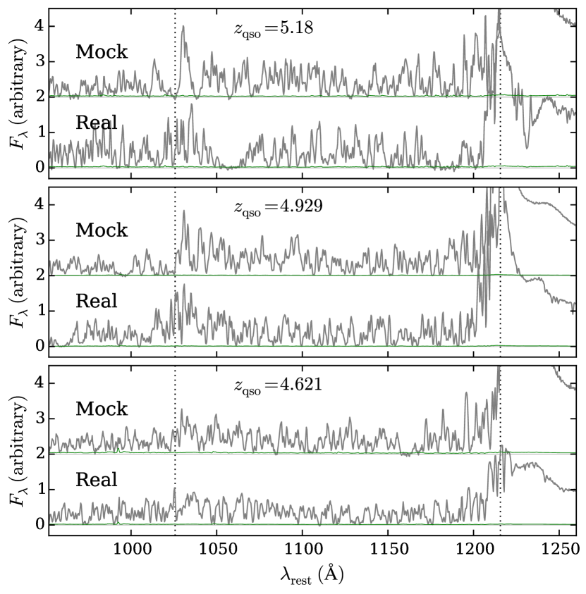
We did not include metal absorption in the mocks. The similarity between the mocks and the real spectra, and the agreement between the correction factors $k_{\mathrm{real}}$ and $k_{\mathrm{found}}$ derived from the mocks and high-resolution spectra suggest their inclusion is unnecessary.

A.1 High ${\it N}_{\mathrm{HI}}$ DLAs

DLAs in the column density range ${\it N}_{\mathrm{HI}}=10^{21-21.8}$ cm^-2 make the dominant contribution to $\rm\Omega_{\rm HI}$, and it is thus important to correctly measure the uncertainty in $k_{\mathrm{real}}$ and $k_{\mathrm{found}}$ for this ${\it N}_{\mathrm{HI}}$ range. There are only $\sim 10$ DLAs in this column density range in both the mocks and the high-resolution sample, so the uncertainties in this correction are large. Therefore we generated further mocks with an enhanced incidence rate of high ${\it N}_{\mathrm{HI}}$ systems. We did this by generating 10 times more mocks than were used above, using the same line distribution. Due to time constraints, we were unable to search by eye every one of these mocks. Instead we selected just 100 spectra: the 50 containing the highest ${\it N}_{\mathrm{HI}}$ DLAs, and a further 50 selected at random from the remainder. This formed a sample of 100 new mock spectra which we searched for high ${\it N}_{\mathrm{HI}}$ systems. 50 were included without requiring a DLA to present so that when scanning the spectra by eye, the searcher would not be certain that every spectrum contains a DLA. The $k_{\mathrm{found}}$, $k_{\mathrm{real}}$ values found by including these extra sightlines into our mock sample are shown in Figures 16 and 17. These show that the probability of a spurious DLA at ${\it N}_{\mathrm{HI}}>10^{21}$ cm^-2 is just 1%–5%, using binomial statistics with

The $\log{\it N}_{\mathrm{HI}}$ and velocity differences between the candidate and true values are shown in Figure 18. This shows that even at high ${\it N}_{\mathrm{HI}}$, there is no strong systematic offset from the true value.

Figure 16: The fraction of true DLAs that were correctly identified by one of the authors (NHMC), $k_{\mathrm{found}}$, as a function of the true redshift and ${\it N}_{\mathrm{HI}}$ found using the mock spectra. This includes the mock sightlines with additional strong ${\it N}_{\mathrm{HI}}$ DLAs.

Figure 17: The fraction of non-spurious DLA candidates, $k_{\mathrm{real}}$ by one of the authors (NHMC), as a function of the candidate redshift and ${\it N}_{\mathrm{HI}}$ for the mock spectra. This includes the mock sightlines with additional strong ${\it N}_{\mathrm{HI}}$ DLAs.

Figure 18: The difference between ${\it N}_{\mathrm{HI}}$ estimated for DLA candidates in low resolution spectra ($N_{\mathrm{HI,cand}}$) and $N_{\mathrm{HI,true}}$ measured from mock linelists by one of the authors (NHMC), including the extra sightlines with additional strong ${\it N}_{\mathrm{HI}}$ DLAs. This shows there is no strong systematic offset in the estimated ${\it N}_{\mathrm{HI}}$ as a function of redshift, even for ${\it N}_{\mathrm{HI}}\sim 10^{21.5}$ cm^-2 DLAs.

References

- Astropy Collaboration et al. (2013) Astropy Collaboration et al., 2013, A&A, 558, A33
- Barkana & Loeb (2007) Barkana R., Loeb A., 2007, Reports on Progress in Physics, 70, 627
- Becker et al. (2013) Becker G. D., Hewett P. C., Worseck G., Prochaska J. X., 2013, MNRAS, 430, 2067
- Becker et al. (2015) Becker G. D., Bolton J. S., Madau P., Pettini M., Ryan-Weber E. V., Venemans B. P., 2015, MNRAS, 447, 3402
- Bird et al. (2014) Bird S., Vogelsberger M., Haehnelt M., Sijacki D., Genel S., Torrey P., Springel V., Hernquist L., 2014, MNRAS, 445, 2313
- Bouwens et al. (2012) Bouwens R. J. et al., 2012, ApJ, 752, L5
- Braun (2012) Braun R., 2012, ApJ, 749, 87
- Cameron (2011) Cameron E., 2011, Publ. Astron. Soc. Austral., 28, 128
- Chang et al. (2008) Chang T. C., Pen U. L., Peterson J. B., McDonald P., 2008, Physical Review Letters, 100, 091303
- Cooke et al. (2006) Cooke J., Wolfe A. M., Gawiser E., Prochaska J. X., 2006, ApJ, 652, 994
- Cooke et al. (2010) Cooke R., Pettini M., Steidel C. C., King L. J., Rudie G. C., Rakic O., 2010, MNRAS, 409, 679
- Crighton et al. (2015) Crighton N. H. M., Hennawi J. F., Simcoe R. A., Cooksey K. L., Murphy M. T., Fumagalli M., Prochaska J. X., Shanks T., 2015, MNRAS, 446, 18
- Davé et al. (2013) Davé R., Katz N., Oppenheimer B. D., Kollmeier J. A., Weinberg D. H., 2013, MNRAS, 434, 2645
- Dekel et al. (2009) Dekel A. et al., 2009, Nat, 457, 451
- Delhaize et al. (2013) Delhaize J., Meyer M. J., Staveley-Smith L., Boyle B. J., 2013, MNRAS, 433, 1398
- Duffy et al. (2012) Duffy A. R., Kay S. T., Battye R. A., Booth C. M., Dalla Vecchia C., Schaye J., 2012, MNRAS, 420, 2799
- Ellison et al. (2001) Ellison S. L., Yan L., Hook I. M., Pettini M., Wall J. V., Shaver P., 2001, A&A, 379, 393
- Ellison et al. (2002) Ellison S. L., Yan L., Hook I. M., Pettini M., Wall J. V., Shaver P., 2002, A&A, 383, 91
- Ellison et al. (2010) Ellison S. L., Prochaska J. X., Hennawi J., Lopez S., Usher C., Wolfe A. M., Russell D. M., Benn C. R., 2010, MNRAS, 406, 1435
- Finlator et al. (2012) Finlator K., Oh S. P., Özel F., Davé R., 2012, MNRAS, 427, 2464
- Font-Ribera et al. (2012) Font-Ribera A. et al., 2012, J. Cos. Ast. Phys., 11, 059
- Freudling et al. (2011) Freudling W. et al., 2011, ApJ, 727, 40
- Fumagalli et al. (2011) Fumagalli M., Prochaska J. X., Kasen D., Dekel A., Ceverino D., Primack J. R., 2011, MNRAS, 418, 1796
- Fumagalli et al. (2013) Fumagalli M., O’Meara J. M., Prochaska J. X., Worseck G., 2013, ApJ, 775, 78
- Guimarães et al. (2009) Guimarães R., Petitjean P., de Carvalho R. R., Djorgovski S. G., Noterdaeme P., Castro S., Poppe P. C. D. R., Aghaee A., 2009, A&A, 508, 133
- Hunter (2007) Hunter J. D., 2007, Computing in Science and Engineering, 9, 90
- Jorgenson et al. (2013) Jorgenson R. A., Murphy M. T., Thompson R., 2013, MNRAS, 435, 482
- Jorgenson et al. (2006) Jorgenson R. A., Wolfe A. M., Prochaska J. X., Lu L., Howk J. C., Cooke J., Gawiser E., Gelino D. M., 2006, ApJ, 646, 730
- Kim et al. (2013) Kim T. S., Partl A. M., Carswell R. F., Müller V., 2013, A&A, 552, A77
- Lagos et al. (2014) Lagos C. D. P., Baugh C. M., Zwaan M. A., Lacey C. G., Gonzalez-Perez V., Power C., Swinbank A. M., van Kampen E., 2014, MNRAS, 440, 920
- Lah et al. (2007) Lah P. et al., 2007, MNRAS, 376, 1357
- Lanzetta et al. (1991) Lanzetta K. M., Wolfe A. M., Turnshek D. A., Lu L., McMahon R. G., Hazard C., 1991, ApJS, 77, 1
- Liske et al. (2008) Liske J. et al., 2008, MNRAS, 386, 1192
- Madau & Dickinson (2014) Madau P., Dickinson M., 2014, ARA&A, 52, 415
- Martin et al. (2010) Martin A. M., Papastergis E., Giovanelli R., Haynes M. P., Springob C. M., Stierwalt S., 2010, ApJ, 723, 1359
- Meiring et al. (2011) Meiring J. D. et al., 2011, ApJ, 732, 35
- Ménard & Fukugita (2012) Ménard B., Fukugita M., 2012, ApJ, 754, 116
- Murphy & Liske (2004) Murphy M. T., Liske J., 2004, MNRAS, 354, L31
- Noterdaeme et al. (2009) Noterdaeme P., Petitjean P., Ledoux C., Srianand R., 2009, A&A, 505, 1087
- Noterdaeme et al. (2012) Noterdaeme P. et al., 2012, A&A, 547, L1
- O’Meara et al. (2007) O’Meara J. M., Prochaska J. X., Burles S., Prochter G., Bernstein R. A., Burgess K. M., 2007, ApJ, 656, 666
- O’Meara et al. (2013) O’Meara J. M., Prochaska J. X., Worseck G., Chen H. W., Madau P., 2013, ApJ, 765, 137
- Oppenheimer et al. (2010) Oppenheimer B. D., Davé R., Kereš D., Fardal M., Katz N., Kollmeier J. A., Weinberg D. H., 2010, MNRAS, 406, 2325
- Padmanabhan et al. (2015) Padmanabhan H., Choudhury T. R., Refregier A., 2015, MNRAS, 447, 3745
- Péroux et al. (2003) Péroux C., McMahon R. G., Storrie-Lombardi L. J., Irwin M. J., 2003, MNRAS, 346, 1103
- Péroux et al. (2005) Péroux C., Dessauges-Zavadsky M., D’Odorico S., Sun Kim T., McMahon R. G., 2005, MNRAS, 363, 479
- Pontzen & Pettini (2009) Pontzen A., Pettini M., 2009, MNRAS, 393, 557
- Prochaska & Herbert-Fort (2004) Prochaska J. X., Herbert-Fort S., 2004, PASP, 116, 622
- Prochaska & Wolfe (2009) Prochaska J. X., Wolfe A. M., 2009, ApJ, 696, 1543
- Prochaska et al. (2005) Prochaska J. X., Herbert-Fort S., Wolfe A. M., 2005, ApJ, 635, 123
- Prochaska et al. (2008) Prochaska J. X., Hennawi J. F., Herbert-Fort S., 2008, ApJ, 675, 1002
- Prochaska et al. (2009) Prochaska J. X., Worseck G., O’Meara J. M., 2009, ApJ, 705, L113
- Prochaska et al. (2010) Prochaska J. X., O’Meara J. M., Worseck G., 2010, ApJ, 718, 392
- Prochaska et al. (2014) Prochaska J. X., Madau P., O’Meara J. M., Fumagalli M., 2014, MNRAS, 438, 476
- Rafelski et al. (2012) Rafelski M., Wolfe A. M., Prochaska J. X., Neeleman M., Mendez A. J., 2012, ApJ, 755, 89
- Rafelski et al. (2014) Rafelski M., Neeleman M., Fumagalli M., Wolfe A. M., Prochaska J. X., 2014, ApJ, 782, L29
- Rao et al. (2006) Rao S. M., Turnshek D. A., Nestor D. B., 2006, ApJ, 636, 610
- Rhee et al. (2013) Rhee J., Zwaan M. A., Briggs F. H., Chengalur J. N., Lah P., Oosterloo T., Hulst T. v. d., 2013, MNRAS, 435, 2693
- Rudie et al. (2013) Rudie G. C., Steidel C. C., Shapley A. E., Pettini M., 2013, ApJ, 769, 146
- Russell et al. (2006) Russell D. M., Ellison S. L., Benn C. R., 2006, MNRAS, 367, 412
- Saslaw (1989) Saslaw W. C., 1989, ApJ, 341, 588
- Shull et al. (2012) Shull J. M., Stevans M., Danforth C. W., 2012, ApJ, 752, 162
- Songaila & Cowie (2010) Songaila A., Cowie L. L., 2010, ApJ, 721, 1448
- Storrie-Lombardi & Wolfe (2000) Storrie-Lombardi L. J., Wolfe A. M., 2000, ApJ, 543, 552
- Storrie-Lombardi et al. (1996) Storrie-Lombardi L. J., McMahon R. G., Irwin M. J., 1996, MNRAS, 283, L79
- Suzuki et al. (2005) Suzuki N., Tytler D., Kirkman D., O’Meara J. M., Lubin D., 2005, ApJ, 618, 592
- Tescari et al. (2009) Tescari E., Viel M., Tornatore L., Borgani S., 2009, MNRAS, 397, 411
- Vladilo et al. (2008) Vladilo G., Prochaska J. X., Wolfe A. M., 2008, A&A, 478, 701
- Wolfe et al. (1995) Wolfe A. M., Lanzetta K. M., Foltz C. B., Chaffee F. H., 1995, ApJ, 454, 698
- Wolfe et al. (2005) Wolfe A. M., Gawiser E., Prochaska J. X., 2005, ARA&A, 43, 861
- Worseck & Prochaska (2011) Worseck G., Prochaska J. X., 2011, ApJ, 728, 23
- Worseck et al. (2014) Worseck G. et al., 2014, MNRAS, 445, 1745
- Wyithe & Loeb (2008) Wyithe J. S. B., Loeb A., 2008, MNRAS, 383, 606
- Zafar et al. (2013) Zafar T., Péroux C., Popping A., Milliard B., Deharveng J. M., Frank S., 2013, A&A, 556, A141
- Zwaan et al. (2005) Zwaan M. A., Meyer M. J., Staveley-Smith L., Webster R. L., 2005, MNRAS, 359, L30