Emergent geometry of membranes
Mathias Hudoba de Badyn, Joanna L. Karczmarek, Philippe Sabella-Garnier and Ken Huai-Che Yeh
Department of Physics and Astronomy
University of British Columbia
Vancouver, Canada

In work [1], a surface embedded in flat $\mathbb{R}^{3}$ is associated to any three hermitian matrices. We study this emergent surface when the matrices are large, by constructing coherent states corresponding to points in the emergent geometry. We find the original matrices determine not only shape of the emergent surface, but also a unique Poisson structure. We prove that commutators of matrix operators correspond to Poisson brackets. Through our construction, we can realize arbitrary noncommutative membranes: for example, we examine a round sphere with a non-spherically symmetric Poisson structure. We also give a natural construction for a noncommutative torus embedded in $\mathbb{R}^{3}$. Finally, we make remarks about area and find matrix equations for minimal area surfaces.

1 Introduction

String theory contains many hints that spacetime might be a more complicated object—possibly even an emergent one—than a manifold. Most of our understanding about non-perturbative string theory comes from the study of D-branes, extended objects that strings are allowed to end on. When $N$ identical D-branes are considered, their coordinate positions are described by $N\times N$ hermitian matrices. If these matrix coordinates are simultaneously diagonalizable, their eigenvalues are easily interpreted as the positions of the D-branes. When they are not, as is the situation generically, the D-brane positions are not well defined, even in the classical $\hbar\rightarrow 0$ limit. Thus, D-branes do not ‘view’ spacetime in the same way that ordinary point particles do. The standard string theoretic interpretation of such ‘fuzzy’ configurations through the so-called dielectric effect [2], where lower dimensional D-branes ‘blow up’ to form higher dimensional D-brane. Lack of locality is related to the lower dimensional D-branes being ‘smeared’ over the worldvolume of a higher dimensional emergent object.

In most previous work, explicit geometric interpretation of the matrix coordinates as a higher dimensional object has been limited to simple and highly symmetric geometries, such as planes, tori and spheres. In their paper, [1], take this one step further: using the BFSS model they found a geometric interpretation of three matrix coordinates as a co-dimension one surface embedded in three dimension. The argument was to consider a stack of D0-branes at an orbifold point, and then introduce an extra probe brane into the system. By considering a fermionic string stretching between the stack and the probe brane, the emergent surface was defined as the locus of possible positions for the probe brane where the stretched string has a massless mode (indicating that the string has zero length). This lead to the following effective Hamiltonian:

$$H_{\mathrm{eff}}(x_{i})=\sum_{i=1,2,3}\sigma^{i}\otimes\left(X_{i}-x_{i}\right)~{},$$ (1)

where $X_{i}$ for $i=1,2,3$ are Hermitian, $N\times N$, matrices corresponding to the positions of the stack of D0-branes in a three dimensional flat transverse space, and $x_{i}$ are the positions of the probe brane. The fermionic mode is massless when $H_{\mathrm{eff}}$ has a zero eigenvalue. Thus, the surface corresponding to the three matrices $X_{i}$ is given by the polynomial equation $\det(H_{\mathrm{eff}}(x_{i}))=0$. This defines a co-dimension one surface in flat $\mathbb{R}^{3}$ space parametrized by $(x_{1},x_{2},x_{3})$.

We use equation (1) as the starting point for a concrete and explicit study of geometry of the emergent surface, identifying zero eigenvectors of $H_{\mathrm{eff}}$ with coherent states underlying noncommutative geometry of the emergent surface [9]. We focus on configurations where a smooth and well-defined surface arises from matrices with a large size $N$. Rather than assume it a priori, we prove a correspondence principle between matrix commutators and a unique Poisson bracket on the emergent surface arising from the matrix configuration $(X_{1},X_{2},X_{3})$. This explicit correspondence makes the usual procedure of going from matrix models to surfaces much less ad hoc, which might be of use when quantizing membrane actions by replacing them with a matrix model. We demostrate how easy it is to construct surfaces with desired properties using our approach on several nontrivial examples, including the torus.

Our approach is most similar to that espoused in [4] (see also [5] and references therein), but with an explicit construction for the coherent states associated with points on the surface. The results can also be thought of as a concrete realization of the abstract idea in the classic work by Kontsevich, [6]. Other work includes [7, 8], though our construction appears more general as it allows us to vary the local noncommutativity independent of the shape of the surface.

For most of the paper, we focus on the following question: under what conditions would a sequence of noncommutative geometries, each arising from a matrix configuration $(X_{1},X_{2},X_{3})$ and labeled by an increasing matrix size $N$, converge to a smooth limit? which quantities characterize the surface in this limit?

Since the polynomial equation $\det(H_{\mathrm{eff}}(x_{i}))=0$ has degree $2N$, generically, the locus of its solutions does not need to be smooth in the large $N$ limit. When some generic matrices $X_{i}$ are scaled so that the range of their eigenvalue distributions remains finite at large $N$, the resulting surface is generically quite complicated and does not have a large $N$ limit. As a simple (but not generic) example, let $X_{i}=\mathrm{diag}(\sigma_{i}+a_{i}^{1},\ldots,\sigma_{i}+a_{i}^{N})$, where $\sigma_{i}$ are the Pauli matrices and $a_{i}^{k}$ are real numbers. The resulting surface is a union of $N$ spheres of radius 1 each centered at $(a_{1}^{k},a_{2}^{k},a_{3}^{k})$ for $k$ from 1 to $N$. There is no sense in which the surface achieves a well-defined large $N$ limit. In the degenerate case where all $a_{i}^{k}$ are zero, the surface is a single sphere of radius one centered at the origin. However, it still does not correspond to a smooth geometry, rather, it is a very fuzzy sphere with SU(N) symmetry. To obtain a smooth geometry, we can instead consider $X_{i}=L_{i}/J$, with $L_{i}$ forming the irreducible representation of SU(2) with spin $J$ (this is the standard construction of the noncommutative sphere, see section 3.2 for details). This sphere has radius $1$ independent of $J$. As $N=2J+1\rightarrow\infty$, the noncommutative sphere reproduces the ordinary one.

When the the large $N$ limit exists and is smooth, the emergent surface will be characterized by its geometry (the embedding into flat $\mathbb{R}^{3}$ space) and by a Poisson structure defining (together with $N$) a noncommutative geometry in the large $N$ limit. In section 2, we will make some definitions and introduce our approach. In section 3, we will analyze, analytically and numerically, a series of examples from which a general picture will emerge. In section 4 we will prove the correspondence principle and discuss smoothness conditions which determine how large $N$ has to be for a given noncommutative surface to be well described by the corresponding matrices. In section 5, we will discuss the issue of area and derive the matrix equation for minimal area surfaces. In section 6, we construct a smooth torus embedded in $\mathbb{R}3$. Finally, in section 7 we discuss topics for future work.

2 Basic setup

Since our emergent surface is given by the locus of points where the effective Hamiltonian $H_{\mathrm{eff}}$ in equation (1) has a zero eigenvalue, for each point $p$ on the surface $H_{\mathrm{eff}}$ has (properly normalized) zero eigenvector $|\Lambda_{p}\rangle$:

$$H_{\mathrm{eff}}|\Lambda_{p}\rangle=0~{}.$$ (2)

The above equation defines (in non-degenerate cases) a two dimensional surface embedded in three dimensional space. We will take the three dimensional space to be flat; the metric on the emergent two dimensional surface will then just be the pullback from the flat three dimensional metric.

It is instructive to rewrite the above equation in a slightly different way:

$$\sum_{i=1,2,3}\left(\sigma^{i}\otimes X_{i}\right)|\Lambda_{p}\rangle=\sum_{i=1,2,3}\left(\sigma^{i}\otimes x_{i}\right)|\Lambda_{p}\rangle~{}.$$ (3)

This equation can be thought of as an analogue of an eigenvalue equation: while the three matrices $X_{i}$ cannot be simultaneously diagonalized, the above equation says that if we double the dimensionality of the space under consideration, there are special vectors $|\Lambda_{p}\rangle$ on which the action of $X_{i}$ is described by only three parameters. In analogy with the Berezin approach to noncommutative geometry [9], we would like to think of these states as coherent states corresponding to points on the noncommutative surface.. In the Berezin approach, every point $p$ is associated with a coherent state $|\alpha_{p}\rangle$. One then defines a map from any $\hat{A}$ to a function on the noncommutative surface via $s(\hat{A})=\langle\alpha_{p}|\hat{A}|\alpha_{p}\rangle$. This function is usually called the symbol map. From it one can find the corresponding star-product and the rest of the usual machinery of noncommutative geometry.

The first difficulty we see with $\Lambda_{p}$ being the coherent state is that our operators $X_{i}$ (and their functions) cannot be seen as acting on $|\Lambda_{p}\rangle$ due to dimension mismatch. We can simply ‘double’ these operators by using $\boldsymbol{1}_{2}\otimes X_{i}$ instead ($\boldsymbol{1}_{k}$ will denote the $k\times k$ identity matrix). However, while it is true that

$$\langle\Lambda_{y}|~{}\boldsymbol{1}_{2}\otimes X_{i}~{}|\Lambda_{p}\rangle=x_{i}(\sigma)~{},$$ (4)

this approach is somewhat artificial. We will see that there is a more natural solution: for large $N$, when the emergent noncommutative surface is smooth in the sense discussed in the Introduction, the eigenvector $|\Lambda_{p}\rangle$ is approximately a product, $|\Lambda_{p}\rangle=|a\rangle\otimes|\alpha_{p}\rangle$, where $|\alpha_{p}\rangle$ is $N$-dimensional and $|a\rangle$ is 2-dimensional. In the next section, we will examine examples in which the zero eigenvectors of $H_{\mathrm{eff}}$ do factorize in this manner when $N$ is large. A way to measure the extent of the factorization is to write any (2$N$)-dimensional vector as

$$|\Lambda_{p}\rangle=\left[\begin{array}[]{c}|\alpha_{1}\rangle\\ \hline\cr|\alpha_{2}\rangle\end{array}\right]~{},$$ (5)

with $||\alpha_{1}||^{2}+||\alpha_{2}||^{2}=1$, and to define

$$A_{p}=\sqrt{||\alpha_{1}||^{2}||\alpha_{2}||^{2}-|\langle\alpha_{1}|\alpha_{2}\rangle|^{2}}~{},$$ (6)

which can be thought of as the area of the parallelogram defined by the two vectors $|\alpha_{1}\rangle$ and $|\alpha_{2}\rangle$. We will be arguing that, in the large $N$ limit, $A_{p}$ is of order $N^{-1/2}$, implying that $|\alpha_{1}\rangle$ and $|\alpha_{2}\rangle$ are indeed approximately parallel and we can write

$$|\Lambda_{p}\rangle=\left[\begin{array}[]{c}a|\alpha_{p}\rangle\\ \hline\cr b|\alpha_{p}\rangle\end{array}\right]+\mathcal{O}(1/\sqrt{N})~{}.$$ (7)

(By $\mathcal{O}(1/N^{-1/2})$ we mean that the norm of the correction vector decreases with increasing $N$ like $1/N^{-1/2}$.) It will then be the $N$-dimensional vector $|\alpha_{p}\rangle$ that will play the role of a coherent state corresponding to point $p$.

The complex coefficients $(a,b)$ of the 2-vector $|a\rangle$ determine the direction of the normal vector $n$ at point $p$ given by $(x_{1},x_{2},x_{3})$. To see this, consider moving $p$ slightly to $(x_{1}+dx_{1},x_{2}+dx_{2},x_{2}+dx_{3})$, where $(dx_{1},dx_{2},dx_{3})$ is an infinitesimal tangent to the surface. First order perturbation theory implies that to maintain the condition that $H_{\mathrm{eff}}$ has a zero eigenvalue, we must have $\langle\Lambda_{p}|dH_{\mathrm{eff}}|\Lambda_{p}\rangle=\langle\Lambda_{p}|\sigma^{i}\otimes(-dx_{i})|\Lambda_{p}\rangle=0$. Thus $dx_{i}~{}\langle\Lambda_{p}|\sigma^{i}\otimes{\mathbf{1}}_{N}|\Lambda_{p}\rangle=0$, implying that

$$n_{i}:=\langle\Lambda_{p}|~{}\sigma^{i}\otimes{\mathbf{1}}_{N}~{}|\Lambda_{p}\rangle$$ (8)

is a vector normal to the surface at a point $p$. This is an exact statement and does not rely on our factorization assumption. Incidentally, we have the formula $|n|^{2}=1-4A_{p}^{2}$, so the normal vector is close to being a unit normal when the factorization condition holds. When we use equation (7), we obtain that the normal vector is $(\bar{a}b+a\bar{b},i(a\bar{b}-\bar{a}b),\bar{a}a-\bar{b}b)$. Thus, the coefficients $(a,b)$ fix the direction of the normal vector. Conversely, the normal vector fixes the coefficients $(a,b)$ up to an overall irrelevant phase.

Next, we will try to define local noncommutativity on the surface. The local noncommutativity can be thought of in two different ways: the size of ‘fuzziness’ (or uncertainty) of the operators $X_{i}$ in the state $|\Lambda_{p}\rangle$, or the size of the commutators of the $X_{i}$s when acting on $|\Lambda_{p}\rangle$. In a coherent state, these two notions should be equal, and they turn out to be equal here, strengthening our case that $|\Lambda_{p}\rangle$ can be thought of as a coherent state. Using $\sigma^{i}\sigma^{j}=i\epsilon^{ijk}\sigma^{k}=-\sigma^{j}\sigma^{i}$ for $i\neq j$ and $\sigma_{i}^{2}=1$, we have a nice little identity

$$(H_{\mathrm{eff}})^{2}=\boldsymbol{1}_{2}\otimes\sum_{i}(X_{i}-x_{i})^{2}~{}+~{}{{1\over 2}}i\epsilon_{ijk}\sigma_{i}\otimes[X_{j},X_{k}]~{}.$$ (9)

Then, since $\langle\Lambda_{p}|(H_{\mathrm{eff}})^{2}|\Lambda_{p}\rangle=0$, we have

$$\langle\Lambda_{p}|\boldsymbol{1}_{2}\otimes\sum_{i}(X_{i}-x_{i})^{2}|\Lambda_{p}\rangle=-{{1\over 2}}i\epsilon_{ijk}~{}\langle\Lambda_{p}|\sigma_{i}\otimes[X_{j},X_{k}]|\Lambda_{p}\rangle~{}.$$ (10)

When the vector $|\Lambda\rangle$ is indeed a product, we can use equation (7) to make the following definition: the local noncommutativity on the noncommutative surface is

$$\theta=\langle\alpha_{p}|\sum_{i}(X_{i}-x_{i})^{2}|\alpha_{p}\rangle={{1\over 2}}\epsilon_{ijk}~{}\theta_{ij}~{}n^{k}~{},$$ (11)

where

$$\theta_{ij}:=\langle\alpha_{p}|-i[X_{i},X_{j}]|\alpha_{p}\rangle~{}.$$ (12)

The LHS of expression (11) is a sum of squares of uncertainties in the operators $X_{i}$, while the RHS depends on the commutators. The particular combination of commutators is of interest: with our factorization assumption, the commutator term picks up only the contributions that are transverse to the normal, for example, if the normal vector $n$ is pointing in the $x_{3}$ direction, only $[X_{1},X_{2}]$ contribute to $\theta$. In fact, it will turn out that, in the large $N$ limit, $\epsilon_{ijk}\theta_{ij}$ is nearly parallel to $n_{k}$. Thus, we can also write $\theta$ as

$$\theta=\langle\alpha_{p}|~{}\sqrt{\sum_{i\neq j}-[X_{i},X_{j}]^{2}}~{}|\alpha_{p}\rangle~{}.$$ (13)

As for the first expression in equation (11), it will turn out that if we take the normal vector to point along the $x_{3}$ direction, we have $\langle\alpha|(X_{1}-x_{1})^{2}|\alpha\rangle\approx\langle\alpha|(X_{2}-x_{2})^{2}|\alpha\rangle\gg\langle\alpha|(X_{3}-x_{3})^{2}|\alpha\rangle$, so the coherent state is ‘flattened’ to lie predominantly in the 1-2-plane and balanced (‘round’).

To flesh out these ideas, we will examine a series of increasingly complex examples. In the process, we will construct the approximate eigenvector $|\alpha_{p}\rangle$ and study corrections to the large $N$ limit described above.

3 Coherent state and its properties

We will make the following choice for the Pauli matrices $\sigma_{i}$

$$\sigma^{1}=\begin{bmatrix}0&1\\ 1&0\end{bmatrix}~{},~{}~{}~{}\sigma^{2}=\begin{bmatrix}0&-i\\ i&0\end{bmatrix}~{},~{}~{}~{}\sigma^{3}=\begin{bmatrix}1&0\\ 0&-1\end{bmatrix}~{}.$$ (14)

In this convention, we can write $H_{\mathrm{eff}}$ in a natural way in terms of $N\times N$ blocks

$$H_{\mathrm{eff}}=\left[\begin{array}[]{c|c}X_{3}-x_{3}&(X_{1}-iX_{2})-(x_{1}-ix_{2})\\ \hline\cr(X_{1}+iX_{2})-(x_{1}+ix_{2})&-(X_{3}-x_{3})\end{array}\right]~{},$$ (15)

We will now examine a series of examples of increasing complexity, always focusing on a point where the normal vector to the surface is pointing straight up (in the $x_{3}$ direction).

Our final conclusion will be that at such a point, the zero-eigenvector of $H_{\mathrm{eff}}$ has the form given in equation (7):

$$|\Lambda\rangle=\left[\begin{array}[]{c}|\alpha\rangle\\ \hline\cr 0\end{array}\right]~{}+~{}{\cal O}\left(N^{-1/2}\right).$$ (16)

$|\alpha\rangle$ with $\langle\alpha|\alpha\rangle=1$ will be the coherent state associated with this particular point on the surface, $-i\langle\alpha|[X_{1},X_{2}]|\alpha\rangle$ will correspond to the local value of noncommutativity at this point. This result is easily generalizable to any orientation of the surface using an SU(2) rotation of the Pauli matrices.

3.1 Example: noncommutative plane

Consider the example of a noncommutative plane: let $X_{3}=0$, and let $[X_{1},X_{2}]=i\theta$. Out of necessity, $X_{1}$ and $X_{2}$ are infinite dimensional operators. This will not be the case when we are considering compact noncommutative surfaces. We have

$$H_{\mathrm{eff}}=\left[\begin{array}[]{c|c}-x_{3}&A^{\dagger}-\bar{\alpha}\\ \hline\cr A-\alpha&x_{3}\end{array}\right]~{},$$ (17)

where $A=X_{1}+iX_{2}$, $A$ and $A^{\dagger}$ are the lowering and raising operators of a harmonic oscillator with $[A,A^{\dagger}]=2\theta$, and $\alpha=x_{1}+ix_{2}$. The lowering operator $A$ has eigenstates $|\alpha\rangle$, called the coherent states, corresponding to every complex number $\alpha$: $A|\alpha\rangle=\alpha|\alpha\rangle$. We thus have a zero eigenvector for $H_{\mathrm{eff}}$ with $x_{3}=0$:

$$|\Lambda(\alpha)\rangle=\left[\begin{array}[]{c}|\alpha\rangle\\ \hline\cr 0\end{array}\right]~{}.$$ (18)

The noncommutative plane is flat and has constant noncommutativity. The normal vector is $\langle\Lambda|\sigma^{i}\otimes{\mathbf{1}}|\Lambda\rangle=(0,0,1)$ and we have $-i\langle\alpha[X_{1},X_{2}]\alpha\rangle=\theta$.

The importance of this example is that, locally and in the large $N$ limit, any noncommutative surface should look like the noncommutative plane. This is the observation that will allow us to write our definition of a large $N$ (smooth) limit.

3.2 Example: noncommutative sphere

Here we have $X_{i}=L_{i}/J$ where $L_{i}$ form the $N$-dimensional irrep of SU(2): $[L_{i},L_{j}]=i\epsilon_{ijk}L_{k}$ and where $J=(N-1)/2$ is the spin. It is useful to consider the usual raising and lowering operators, $L_{\pm}=L_{1}\pm iL_{2}$. Without loss of generality, consider that point on the noncommutative surface which lies on the $x_{3}$ axis. With $x_{1}=x_{2}=0$, $H_{\mathrm{eff}}$ is

$$H_{\mathrm{eff}}=\left[\begin{array}[]{c|c}L_{3}/J-x_{3}&L_{-}/J\\ \hline\cr L_{+}/J&-(L_{3}/J-x_{3})\end{array}\right]~{}.$$ (19)

We will use as a basis the eigenvectors of the $L_{3}$ angular momentum, $|m\rangle$:

$$L_{3}|m\rangle=m|m\rangle~{},~{}~{}m=-J\ldots J~{},~{}~{}\langle m|m\rangle=1~{},~{}~{}J=\frac{N-1}{2}~{}.$$ (20)

It is easy to see that

$$|\Lambda\rangle=\left[\begin{array}[]{c}|J\rangle\\ \hline\cr 0\end{array}\right]$$ (21)

is a zero eigenvector of $H_{\mathrm{eff}}$ if $x_{3}=1$. Thus, the noncommutative sphere has radius 1.

3.3 Looking ahead: polynomial maps from the sphere

A large class of surfaces that can be studied using our tools are surfaces that are generated from polynomials of the normalized SU(2) generators considered above:

$$X_{i}=\mathrm{polynomial}(L_{1}/J,L_{2}/J,L_{3}/J)~{},$$ (22)

where the polynomials in three variables have degrees and coefficients that are independent of $N$. In this case, we expect that at large $N$ the noncommutative surface will approach an algebraic variety given by the image of the unit sphere under the polynomial maps used to construct $X_{i}$.

Concretely, consider a surface $\cal{S}$ in $\mathbb{R}^{3}$ constructed as follows: let $p_{1}$, $p_{2}$ and $p_{3}$ be three polynomials discussed, in three variables $w_{1}$, $w_{2}$ and $w_{3}$. Then, consider the image in $\mathbb{R}^{3}$ under these three polynomial maps of the surface $\sum_{i}(w_{i})^{2}=1$, ie

$${\cal S}=\left\{(x_{1},x_{2},x_{3})~{}|~{}x_{i}=p_{i}(w_{1},w_{2},w_{3})~{}\mathrm{and}~{}\sum_{i}(w_{i})^{2}=1\right\}~{}.$$ (23)

We will restrict our considerations to surfaces which are non-self-intersecting, meaning that the polynomial map is one-to-one. The corresponding noncommutative surface is specified by three $N\times N$ matrices $X_{i}$ which can be written as corresponding polynomial expressions in $L_{i}$:

$$X_{i}=\mathrm{sym}\left(p_{i}(L_{1}/J,L_{2}/J,L_{3}/J)\right)~{},$$ (24)

where, to avoid ambiguity, the ‘sym’ map completely symmetrizes any products of the three non-commuting matrices $L_{i}$. This symmetrization will turn out to play little role in what follows: re-ordering the terms of order $k$ leads to small—suppressed by a power of $J$—corrections in the coefficients of the polynomials of order less than $k$.

Now, consider an arbitrary point $p=(y_{1},y_{2},y_{3})$ on the surface $\cal{S}$. Acting with SO(3) on the space $(x_{1},x_{2},x_{3})$, arrange for the normal vector to $\cal{S}$ at the point $p$ to point along the positive $x_{3}$-direction, and acting with SO(3) on the space $(w_{1},w_{2},w_{3})$, arrange for the pre-image of the point $p$ to be the north pole. It is then necessary that the polynomial maps take a form

$$x_{1} ~{}=~{}y_{1}+c_{1}w_{1}+c_{2}w_{2} +~{}a(w_{3}-1)~{}+~{}p_{1}^{(2)}(w_{1},w_{2},w_{3}-1)~{},$$

$$x_{2} ~{}=~{}y_{2}+c_{3}w_{1}+c_{4}w_{2} +~{}b(w_{3}-1)~{}+~{}p_{2}^{(2)}(w_{1},w_{2},w_{3}-1)~{},$$ (25)

$$x_{3} ~{}=~{}y_{3} +~{}c(w_{3}-1)~{}+~{}p_{3}^{(2)}(w_{1},w_{2},w_{3}-1)~{},$$

where $c_{i}$, $a$, $b$ and $c$ are real numbers and where $p_{i}^{(2)}(\cdot)$ are polynomials of degree at least 2. To avoid a coordinate singularity, we should have $c_{1}c_{4}-c_{2}c_{3}\neq 0$. Then, using a rotation of $w_{1}$ and $w_{2}$ (in other words, rotating the unit sphere around the north pole), we can set $c_{3}$ zero and $c_{4}>0$. Finally we can take $c_{1}>0$ by adjusting the sign of $w_{1}$ if necessary.

The four coefficients $c_{1},\ldots,c_{4}$ determine the metric on the surface in terms of the metric on the sphere. If the metric on the sphere is $g_{S^{2}}$, then the induced metric on the surface is

$$g_{ab}:=\left({\mathbf{C}}^{T}g_{S^{2}}{\mathbf{C}}\right)_{ab}~{},~{}\mathrm{where}~{}{\mathbf{C}}=\left[\begin{array}[]{cc}c_{1}&c_{2}\\ c_{3}&c_{4}\end{array}\right]~{}.$$ (26)

This implies that $\sqrt{\det g}/\sqrt{\det g_{S^{2}}}=\det{\mathbf{C}}$, which is a useful fact to keep in mind.

Without loss of generality, we are interested in the eigenvector of $H_{\mathrm{eff}}$ at a point such that the normal to the surface is pointing along the 3-direction. We now want to show that the corresponding zero-eigenvector of $H_{\mathrm{eff}}$ has the form shown in equation (16).

Before we plunge into analyzing this rather general setup, we will narrow the example down to a simpler one which nonetheless contains most of the salient features of our general approach.

3.4 Example: noncommutative ellipsoid

Here, we will consider a stretched noncommutative sphere. The most generic closed quadratic surface in three dimensions is an ellipsoid, with three orthogonal major axes positioned at some arbitrary position in the three dimensional space under consideration. In other words, we will allow $X_{i}$ to be arbitrary linear combinations of $L_{1}/J$, $L_{2}/J$ and $L_{3}/J$. Under the general framework described above, this amounts to setting the higher degree polynomials $p_{i}^{(2)}$ to zero:

$$X_{i}=\mathbf{A}_{ij}L_{j}/J,~{}~{}\mathrm{where~{}~{}}\mathbf{A}=\left[\begin{array}[]{ccc}c_{1}&c_{2}&a\\ 0&c_{4}&b\\ 0&0&c\end{array}\right]~{}.$$ (27)

The classical, or infinite $N$, surface is given by $x_{i}=\mathbf{A}_{ij}w_{j}$ with $\sum_{i}(w_{i})^{2}=1$. It is easy to check that at a point $x=(a,b,c)$, this surface has a normal vector which is pointing along the positive $x_{3}$-direction. We will therefore consider finding the exact location of the surface at a point with $x=(a,b,x_{3})$ where we expect $z_{3}$ to be close to c. We have

$$H_{\mathrm{eff}}(x_{3})=\left[\begin{array}[]{c|c}c\frac{L_{3}}{J}-x_{3}&A^{\dagger}~{}+~{}(a-ib)(L_{3}/J-1)\\ \hline\cr A~{}+~{}(a+ib)(L_{3}/J-1)&-\left(c\frac{L_{3}}{J}-x_{3}\right)\end{array}\right]~{},$$ (28)

where

$$A=\frac{(c_{1}+c_{4})-ic_{2}}{2J}L_{+}+\frac{(c_{1}-c_{4})+ic_{2}}{2J}L_{-}~{}.$$ (29)

What we need to do is find a good approximation to the zero eigenvector of $H_{\mathrm{eff}}(x_{3})$, together with an estimate for the (hopefully small) difference $x_{3}-c$. We conjecture that such a vector is in some way similar to that in equation (21): the ‘top part’ is large compared with the ‘bottom part’ and is dominated by components with the largest eigenvalues of $J_{3}$. To achieve this, write $H_{\mathrm{eff}}$ as a sum of two parts:

$$H_{\mathrm{eff}}(x_{3})=\left[\begin{array}[]{c|c}0&A^{\dagger}\\ \hline\cr A&0\end{array}\right]~{}+~{}\left[\begin{array}[]{c|c}c\frac{L_{3}}{J}-x_{3}&(a-ib)\left(\frac{L_{3}}{J}-1\right)\\ \hline\cr(a+ib)\left(\frac{L_{3}}{J}-1\right)&-\left(c\frac{L_{3}}{J}-x_{3}\right)\end{array}\right]~{}.$$ (30)

If we focus on vectors whose $N$-dimensional sub-vectors are dominated by components with large $L_{3}$ eigenvalues, then the first part can be thought of as being of order $N^{-1/2}$ while the second part is of order $N^{-1}$. Our attempt to find an approximate eigenvector of $H_{\mathrm{eff}}(x_{3})$ will treat the second part as a small perturbation on the first part, suppressed by $N^{-1/2}$.

Consider now a vector—which we will show to be either a zero eigenvector of $A$ or very close to such, and which will thus be an approximate zero-eigenvector of $H_{\mathrm{eff}}(x_{3})$—given by

$$\left[\begin{array}[]{c}|\alpha\rangle\\ \hline\cr 0\end{array}\right]~{},$$ (31)

where

$$|\alpha\rangle=\frac{1}{\sqrt{K}}\sum_{m=0}^{\lfloor J\rfloor}~{}\left(\xi^{m}~{}\sqrt{\prod_{k=1}^{m}\frac{(2k-1)(2J-2k+2)}{(2k)(2J-2k+1)}}\right)~{}|J-2m\rangle~{},$$ (32)

with $\xi$ is given by

$$\xi=-\frac{c_{1}-c_{4}+ic_{2}}{c_{1}+c_{4}-ic_{2}}~{}.$$ (33)

The normalization constant, for which $\langle\alpha|\alpha\rangle=1$, can be computed in the large $J$ limit as

$$K = \sum_{m=0}^{\lfloor J\rfloor}~{}\left(\left|\xi\right|^{2m}~{}\prod_{k=1}^{m}\frac{(2k-1)(2J-2k+2)}{(2k)(2J-2k+1)}\right)$$ (34)

$$\approx 1+\sum_{m=1}^{\infty}~{}\left(\left|\xi\right|^{2m}~{}\frac{(2m-1)!!}{(2m)!!}\right)~{}~{}=~{}~{}1+2\sum_{m=1}^{\infty}|\xi/2|^{2m}\frac{(2m-1)!}{m!(m-1)!}$$ (35)

$$= 1+\frac{|\xi|^{2}}{1-|\xi|^{2}+\sqrt{1-|\xi|^{2}}}~{}~{}=~{}\frac{1}{\sqrt{1-|\xi|^{2}}}~{},$$ (36)

where it is important that $|\xi|<1$, which can be seen from the explicit form in equation (33). For completeness, let us state that

$$1-|\xi|^{2}=\frac{4\det{\mathbf{C}}}{\|{\mathbf{C}}\|^{2}+2\det{\mathbf{C}}}~{},$$ (37)

or

$$\frac{1-|\xi|^{2}}{1+|\xi|^{2}}=\frac{2\det{\mathbf{C}}}{\|{\mathbf{C}}\|^{2}}~{}.$$ (38)

Writing $|\xi|$ in terms of rotational invariants of the matrix $\mathbf{C}$ gives a clear geometric interpretation this is quantity: it is a measure of how much the map in equation (27) distorts the aspect ratio at the point we are interested in.

With a short calculation we see that $A|\alpha\rangle=0$ for integer spin $J$, and that for half-integer spin $J$, we have

$$A|\alpha\rangle = -\frac{c_{1}-c_{4}+ic_{2}}{2J\sqrt{K}}\left(\xi^{J+1/2}\sqrt{\prod_{k=1}^{J-1/2}\frac{(2k-1)(2J-2k+2)}{(2k)(2J-2k+1)}}\right)\sqrt{2J}~{}|-J\rangle$$ (40)

$$= K^{-1/2}(c_{1}-c_{4}+ic_{2})~{}\xi^{J+1/2}~{}\frac{(2J-2)!!}{(2J-1)!!}~{}|-J\rangle~{}.$$ (41)

This is very small: the norm-squared of $A|\alpha\rangle$ is bounded above by

$$b(J):=\left((c_{1}-c_{4})^{2}+(c_{2})^{2}\right)\left|\xi\right|^{2J+1}~{}.$$ (42)

Since $|\xi|<1$, the above quantity goes to zero like $\exp(-(2\ln|\xi|)J)$ for large $J$. Further,

$$\left(\frac{L^{3}}{J}-1\right)|\alpha\rangle=-\frac{1}{\sqrt{K}}\sum_{m=0}^{\lfloor J\rfloor}~{}\frac{2m}{J}~{}\left(\xi^{m}~{}\sqrt{\prod_{k=1}^{m}\frac{(2k-1)(2J-2k+2)}{(2k)(2J-2k+1)}}\right)~{}|J-2m\rangle$$ (43)

and the norm-squared of this vector is equal to

$$\frac{1}{K}\sum_{m=0}^{\lfloor J\rfloor}~{}\left(\frac{2m}{J}\right)^{2}~{}\left(\left|\xi\right|^{2m}~{}\prod_{k=1}^{m}\frac{(2k-1)(2J-2k+2)}{(2k)(2J-2k+1)}\right)~{},$$ (44)

which is bounded above by

$$\sum_{m=0}^{\lfloor J\rfloor}~{}\left(\frac{2m}{J}\right)^{2}~{}\left(\left|\xi\right|^{2m}\right)<J^{-2}\sum_{m=0}^{\infty}~{}\left({2m}\right)^{2}~{}\left(\left|\xi\right|^{2m}\right):=u(J)~{}.$$ (48)

Thus, the bound has the form $u(J)=(\mathrm{function~{}of~{}}\xi)\cdot J^{-2}$.

When $H_{\mathrm{eff}}(x_{3}=c)$ acts on the normalized vector $\left[\begin{array}[]{c}|\alpha\rangle\\ \hline\cr 0\end{array}\right]$, the resulting vector’s norm is, in the large $J$ limit, bounded by $\sqrt{(a^{2}+b^{2}+c^{2})u(J)+b(J)}$, which is itself bounded by a constant times $J^{-1}$. To summarize,

$$\left\|H_{\mathrm{eff}}(c)\left[\begin{array}[]{c}|\alpha\rangle\\ \hline\cr 0\end{array}\right]\right\|~{}<~{}\frac{C(c_{i})}{J}~{},$$ (49)

where $C(c_{i})$ does not depend on $J$ and therefore on $N$.

It follows that $\left[\begin{array}[]{c}|\alpha\rangle\\ \hline\cr 0\end{array}\right]$ is an approximate eigenvector of $H_{\mathrm{eff}}(c)$ and we can place a bound on the corresponding eigenvalue: there exists a vector $\tilde{\Lambda}$ such that

$$H_{\mathrm{eff}}(c)~{}\tilde{\Lambda}=\epsilon\tilde{\Lambda}~{},~{}~{}\mathrm{with}~{}~{}|\epsilon|<\frac{C(c_{i})}{J}~{}.$$ (50)

One can ask the following question: is $\tilde{\Lambda}$ close to $\left[\begin{array}[]{c}|\alpha\rangle\\ \hline\cr 0\end{array}\right]$? To answer this question, we examine the argument that guarantees the existence of $\tilde{\Lambda}$ as above: consider the length squared of $H_{\mathrm{eff}}\left[\begin{array}[]{c}|\alpha\rangle\\ \hline\cr 0\end{array}\right]$ as expanded in eigenvectors of $H_{\mathrm{eff}}$:

$$H_{\mathrm{eff}}\Lambda_{i}=\lambda_{i}\Lambda_{i}~{},~{}~{}~{}~{}H_{\mathrm{eff}}(c)\left[\begin{array}[]{c}|\alpha\rangle\\ \hline\cr 0\end{array}\right]=\sum_{i=1}^{2N}~{}c_{i}\Lambda_{i}~{},~{}~{}~{}~{}\left\|H_{\mathrm{eff}}(c)\left[\begin{array}[]{c}|\alpha\rangle\\ \hline\cr 0\end{array}\right]\right\|^{2}=\sum_{i=1}^{2N}~{}|c_{i}|^{2}|\lambda_{i}|^{2}~{}.$$ (51)

With the bound in equation (49), it is clear that at least one of the eigenvalues $\lambda_{i}$ must be less than $C(c_{i})/J$. Further, if none of the other eigenvalues are small enough, then the eigenvector corresponding to the unique small eigenvalue (which we denoted with $\tilde{\Lambda}$) is very close to $\left[\begin{array}[]{c}|\alpha\rangle\\ \hline\cr 0\end{array}\right]$ itself. For example, if the next smallest eigenvalue $\lambda_{j}$ of $H_{\mathrm{eff}}$ is of order $N^{-1/2}$ (as numerical studies suggest), then the corresponding coefficient $c_{j}$ must be of order $N^{-1/2}$ as well. Therefore, the difference between $\tilde{\Lambda}$ and $\left[\begin{array}[]{c}|\alpha\rangle\\ \hline\cr 0\end{array}\right]$ has length of order $N^{-1/2}$.

Further, we would like to conclude that there exists a third vector $\Lambda$, such that

$$H_{\mathrm{eff}}(c-\zeta)~{}\Lambda=0~{},~{}~{}\mathrm{with}~{}~{}|\zeta|~{}\mathrm{of~{}order}~{}1/J~{},$$ (52)

with $\Lambda$ close to $\tilde{\Lambda}$ and therefore $\left[\begin{array}[]{c}|\alpha\rangle\\ \hline\cr 0\end{array}\right]$. It is possible to argue for this in first order perturbation theory: as we deform $x_{3}$ from $c$ to $c-\zeta$, the eigenvalue of interest changes from $\epsilon$ (in equation (50)) to 0, while the eigenvector changes from $\tilde{\Lambda}$ to $\Lambda$. Since $\epsilon$ is of order $N^{-1}$, $\zeta$ should also be of order $N^{-1}$. Making this analysis rigorous is difficult because, effectively, we are trying to do perturbation theory in $1/N$ while taking a large $N$ limit. Since any sums we take would be over $N$ components, these sums can easily overwhelm any $1/N$ suppression factors. For example, to show that $\Lambda$ is close to $\tilde{\Lambda}$, it is again necessary to bound the remaining spectrum of $H_{\mathrm{eff}}(c)$ away from zero. This is the same bound as was necessary above: the remaining eigenvalues must be bounded away from zero by at least const$/\sqrt{N}$, which seems to be the case when examined numerically.

Instead of attempting a rigorous proof, we will obtain some analytic estimates based on the assumption that the $1/N$ expansion is valid and then confirm these estimates with numerical analysis.

Our idea will be to obtain an analytic result for the leading order contribution to $x_{3}-c$ (which will turn out to be of order $1/N$ as predicted above) and confirm its correctness by comparing with with numerical results. We will also confirm that our approximate eigenvector $\left[\begin{array}[]{c}|\alpha\rangle\\ \hline\cr 0\end{array}\right]$ is a good approximation to the exact zero eigenvector of $H_{\mathrm{eff}}(x_{3})$. Crucial to this approach are two facts: that the eigenvector $|\alpha\rangle$ has components which fall off exponentially with $m$, so that only those components with spin close to the maximum spin $J$ are appreciable, and that the second term in equation (30) is small (of order $1/N$) when acting on these components. Further analysis will then reveal that when the first order correction to the approximate eigenstate is included: $\left[\begin{array}[]{c}|\alpha\rangle\\ \hline\cr|\beta\rangle\end{array}\right]$, the vector $|\beta\rangle$ also has components which fall off exponentially with $m$. We will interpret this as a ‘quasi-locality’ feature of the noncommutative surface.

Now, return to our way of writing $H_{\mathrm{eff}}$ as a sum of two parts in equation (30). Our special vector $\left[\begin{array}[]{c}|\alpha\rangle\\ \hline\cr 0\end{array}\right]$ is an approximate zero eigenvector of the first of these two operators (and an exact zero eigenvector for odd N). Thinking of the second term in equation (30) as a small perturbation in first order perturbation theory, we obtain, to first order, that the change in the eigenvalue is equal to

$$\left[\begin{array}[]{c|c}\langle\alpha|&0\end{array}\right]\left[\begin{array}[]{c|c}c\frac{L_{3}}{J}-x_{3}&(a-ib)\left(\frac{L_{3}}{J}-1\right)\\ \hline\cr(a+ib)\left(\frac{L_{3}}{J}-1\right)&-\left(c\frac{L_{3}}{J}-x_{3}\right)\end{array}\right]\left[\begin{array}[]{c}|\alpha\rangle\\ \hline\cr 0\end{array}\right]$$

$$= \langle\alpha|\frac{L_{3}}{J}c-x_{3}|\alpha\rangle$$

$$= \langle\alpha|\frac{L_{3}}{J}-1|\alpha\rangle c~{}+~{}\langle\alpha|\alpha\rangle(c-x_{3})$$

$$= -\frac{c}{K}\sum_{m=0}^{\lfloor J\rfloor}~{}\frac{2m}{J}~{}\left(\left|\xi\right|^{2m}~{}\prod_{k=1}^{m}\frac{(2k-1)(2J-2k+2)}{(2k)(2J-2k+1)}\right)~{}+~{}(c-x^{3})$$

$$= -\frac{F(\xi,J)}{KJ}~{}+~{}(c-x_{3})~{}.$$

On the last line, we can make an approximation by adding an exponentially small ‘tail’ to the sum, so that the function $F(\xi,J)$ will no longer depend on $J$, making $c-x_{3}$ be of order $J^{-1}$. Explicitly, we have

$$F(\xi,J) :=c\sum_{m=0}^{\lfloor J\rfloor}~{}2m~{}\left(\left|\xi\right|^{2m}~{}\prod_{k=1}^{m}\frac{(2k-1)(2J-2k+2)}{(2k)(2J-2k+1)}\right)$$ (59)

$$\approx c\sum_{m=1}^{\infty}~{}2m~{}\left(\left|\xi\right|^{2m}~{}\frac{(2m-1)!!}{(2m)!!}\right)~{}=~{}c|\xi|\frac{dK}{d|\xi|}~{}.$$ (60)

Taking the change in the eigenvalue to be zero, we get that

$$c-x_{3}~{}=~{}cJ^{-1}\xi\frac{d(\ln K)}{d\xi}~{}=~{}cJ^{-1}\frac{|\xi|^{2}}{1-|\xi|^{2}}~{}=~{}J^{-1}c\frac{(c_{1}-c_{4})^{2}+c_{2}^{2}}{4c_{1}c_{4}}~{}.$$ (61)

We have tested the correctness of this formula numerically, as can be seen in figure 1.

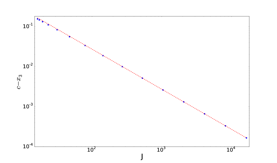
Figure 1: Difference between $x_{3}$ at finite $N$ (obtained numerically) and $c$ (its large $N$ asymptotics), as a function of $N$. The line represents equation (61), which has no free parameters and appears to be an excellent match to the numerical data. In this figure, $(a,b,c)=(1.5,0.5,3)$, $c_{1}=2$, $c_{2}=5$ and $c_{4}=4$. For these values, equation (61) implies that $c-x_{3}=2.71875/J$.

Further, we have checked that $\left[\begin{array}[]{c}|\alpha\rangle\\ \hline\cr 0\end{array}\right]$ is a good approximation to the exact eigenvector. As can be seen in figure 2, the magnitude of the difference decreases as $N^{-1/2}$.

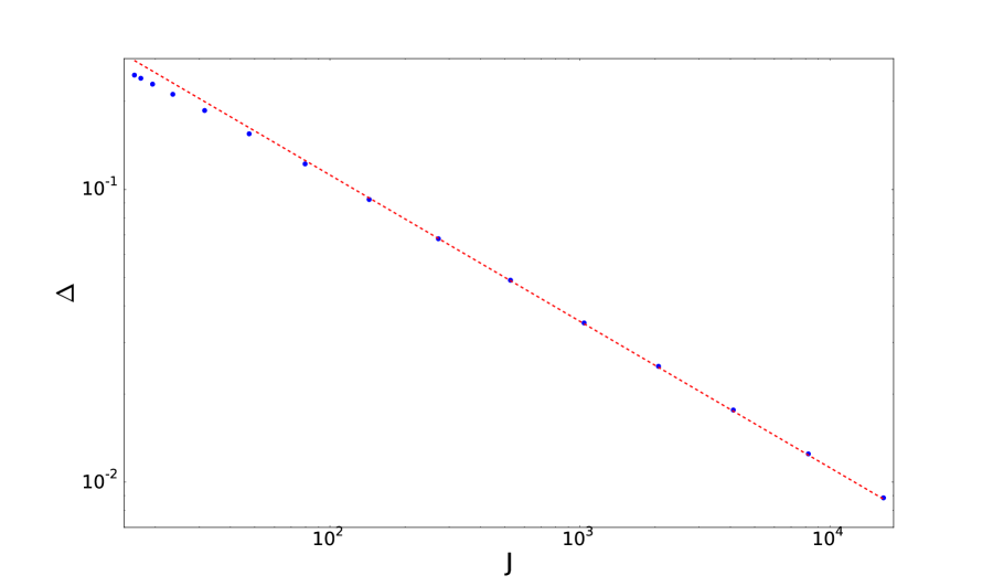
Figure 2: Magnitude, $\Delta$, of the difference between the approximate eigenvector and the exact eigenvector as obtained numerically, for the ellipsoid in figure 1. The straight line, shown to guide the eye, is a best fit to the last few points and corresponds to $\Delta=\frac{1.12}{\sqrt{J}}$.

Once we understand $|\alpha\rangle$, we can ask about the leading correction to the exact eigenvector of $H_{\mathrm{eff}}$. To next order, the eigenvector has a form $\left[\begin{array}[]{c}|\alpha\rangle+|\Delta\alpha\rangle\\ \hline\cr|\beta\rangle\end{array}\right]$, with corrections $|\beta\rangle$ and $|\Delta\alpha\rangle$ that have magnitudes of order no larger than $N^{-1/2}$. Because we are working at a point where the normal vector points ‘up’, we have $\langle\alpha|\beta\rangle=0$. However, generically $\langle\Delta\alpha|\beta\rangle\neq 0$, so the actual normal vector will show a small deviation from this assumed direction. Finally, $A_{p}\approx\sqrt{||\beta||^{2}-|\langle\Delta\alpha|\beta\rangle|^{2}}$.

It is difficult to obtain a closed-form formula for $|\beta\rangle$, and even harder to obtain one for $|\Delta\alpha\rangle$. We should proceed by finding a complete eigenbasis for the first part of $H_{\mathrm{eff}}$ as written in equation (30), and then use standard perturbation theory to obtain the desired result. This is beyond the scope of this paper, so we will resort to less complete methods to obtain some insight into the structure.

The formal expression for $|\beta\rangle$ is

$$|\beta\rangle~{}=~{}(A^{\dagger})^{-1}~{}\left(c\frac{L_{3}}{J}-x_{3}~{}+~{}p^{(2)}_{3}\right)|\alpha\rangle~{}.$$ (62)

This expression is formal because $A^{\dagger}$ might not have an inverse when acting on the above operator. However, we notice that since we already know $x_{3}$, we are able to find, to leading order in $N$, the first nonzero coefficient of $|\beta\rangle$ (which is the coefficient of $|J-1\rangle$). To do so, we take our already computed value of $x_{3}$ and solve this equation:

$$A^{\dagger}|\beta\rangle=-\left(c\frac{L_{3}}{J}-x_{3}\right)|\alpha\rangle~{}.$$ (63)

Once we have the first coefficient, we can substitute it back into the above equation and solve for the next coefficient. Repeating this will in principle yield nearly all components of $|\beta\rangle$ (with exception of the component with the most negative $L_{3}$ eigenvalue).

Explicitly, we obtain that the coefficient of $|J-1\rangle$ in $|\beta\rangle$ is

$$\frac{c-x_{3}}{\sqrt{K}}\frac{\sqrt{2J}}{c_{1}-c_{4}-ic_{2}}~{}.$$ (64)

The magnitude squared of this expression is

$$\frac{c^{2}}{2J}\frac{1}{\det{\mathbf{C}}}\frac{|\xi|^{2}}{(1-|\xi|^{2})^{1/2}}~{}.$$ (65)

We need this expression to be small (compared to 1), since we would like $\|\beta\|\ll\|\alpha\|$. Thus, for nonzero $|\xi|$, how large $J$ needs to be for our analysis to be applicable depends, for example, on $c$. Numerical study confirms equation (65); further, it shows that the ratio of the expression in equation (65) and the total magnitude squared of $|\beta\rangle$ goes to a constant value at large $N$. Thus, $\|\beta\|^{2}$ is proportional to $c^{2}$ and decreases with large $J$ like $J^{-1}$.

We will see in section 4 that corrections shown in equations (61) and (65) are large when $N$ is too small to describe the portion of a given surface with a high curvature.

At the same order, we also get a correction to $|\alpha\rangle$, $|\Delta\alpha\rangle$. A formal expression, similar to the one for $|\beta\rangle$ above,

$$|\Delta\alpha\rangle~{}=~{}A^{-1}\left((a+ib)\left(\frac{L_{3}}{J}-1\right)\right)|\alpha\rangle~{},$$ (66)

does not have a well defined meaning as $\left((a+ib)\left(\frac{L_{3}}{J}-1\right)\right)|\alpha\rangle$ generically has a significant component parallel to $|\alpha\rangle$. It is not possible to solve for coefficients of $|\Delta\alpha\rangle$ in the same way that we solved for those of $|\beta\rangle$; we need a complete perturbation theory treatment. However, using the above expression as a guide to structure at least, we see that the correction $|\Delta\alpha\rangle$ is of order ${\cal O}(N^{-1/2})$, and that it would grow with $a$ and $b$. While the coefficient $c$ determines the local curvature of the surface, the coefficients $a$ and $b$ control how fast the noncommutativity is changing, as we will see in section 3.6.

As we already mentioned, $|\Delta\alpha\rangle$ is not necessarily orthogonal to $|\beta\rangle$, so we will now have a correction to the angle of the normal vector,

$$n_{i}\approx(2\Re\langle\Delta\alpha|\beta\rangle,2\Im\langle\Delta\alpha|\beta\rangle,1)~{}.$$ (67)

Numerical work confirms that the angle between the expected normal vector to the surface (which here points in the $x_{3}$-direction) and the actual normal vector to the surface scales like $N^{-1}$ and grows linearly with the coefficients $a$ and $b$. We will return to this point in section 4.

3.5 Polynomial maps from the sphere

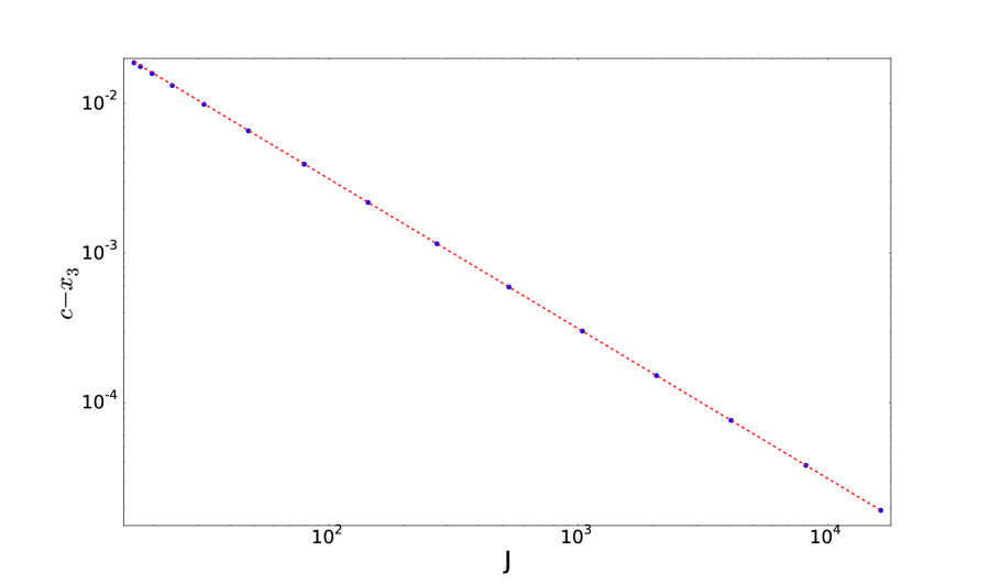
Figure 3: The difference between the actual eigenvalue $x_{3}$ and the classical (large $N$) position $c$ for a generic surface given by $x_{1}=1+w_{1}+0.5w_{3}$, $x_{2}=2w_{2}$, $x_{3}=w_{3}+0.2w_{1}w_{2}$, at a point given by $(w_{1},w_{2},w_{3})=(1/2,1/4,\sqrt{11}/4)$. The line shows equation (80).

Our analysis of a generic polynomial surface will build on the analysis of an ellipsoid. Consider a point of interest such that the normal at this point is pointing in the positive $x_{3}$ direction. Let this point lie at $x_{1}=x_{2}=0$, setting $y_{1}=y_{2}=0$. Without loss of generality, set $y_{3}$ equal to zero as well. This allows us to write $H_{\mathrm{eff}}$ as a sum of two pieces as before:

$$H_{\mathrm{eff}}(x_{3}) = \left[\begin{array}[]{c|c}0&A^{\dagger}\\ \hline\cr A&0\end{array}\right]$$ (70)

$$+ \left[\begin{array}[]{c|c}c\frac{L_{3}}{J}-x_{3}~{}+~{}p^{(2)}_{3}&(a-ib)\left(\frac{L_{3}}{J}-1\right)~{}+~{}p^{(2)}_{1}-ip^{(2)}_{2}\\ \hline\cr(a+ib)\left(\frac{L_{3}}{J}-1\right)~{}+~{}p^{(2)}_{1}+ip^{(2)}_{2}&-\left(c\frac{L_{3}}{J}-x_{3}\right)~{}-~{}p^{(2)}_{3}\end{array}\right]~{}.$$ (73)

$p^{(2)}$ are the polynomials introduced in section 3.3: to leading order, they can be written as

$$p^{(2)}_{k} = d_{k,1}\left(\frac{L_{+}}{J}\right)^{2}+d_{k,2}\left(\frac{L_{-}}{J}\right)^{2}+d_{k,3}\,\frac{L_{+}L_{-}+L_{-}L_{+}}{2J^{2}}$$ (74)

$$= e_{k,1}\left(\frac{L_{1}}{J}\right)^{2}+e_{k,2}\left(\frac{L_{2}}{J}\right)^{2}+e_{k,3}\,\frac{L_{1}L_{2}+L_{2}L_{1}}{2J^{2}}$$ (75)

where $e_{k,1}=d_{k,1}+d_{k,2}+d_{k,3}$, $e_{k,2}=-d_{k,1}-d_{k,2}+d_{k,3}$ and $e_{k,3}=2i(d_{k,1}-d_{k,2})$. Second or higher order polynomials containing at least one power of $L_{3}/J-1$ are either equivalent to polynomials in $L_{1}/J$ and $L_{2}/J$ (from $L_{1}^{2}+L_{2}^{2}+L_{3}^{2}=N^{2}-1$), or subleading, as we will see in a moment.

The vector defined in equation (31) together with $|\alpha\rangle$ given in equation (32) is an approximate zero eigenvector of this more general $H_{\mathrm{eff}}$ as well, as we have confirmed numerically. Generically, $A_{p}$ decreases with large $N$ like $N^{-1/2}$.

Analytically, we first compute the following quantities

$$\langle\alpha|\frac{L_{-}L_{+}}{J^{2}}|\alpha\rangle \approx\frac{2}{J}\frac{|\xi|^{2}}{1-|\xi|^{2}}$$ (76)

$$\langle\alpha|\frac{L_{+}L_{-}}{J^{2}}|\alpha\rangle \approx\frac{2}{J}\frac{1}{1-|\xi|^{2}}$$ (77)

$$\langle\alpha|\frac{L_{+}L_{+}}{J^{2}}|\alpha\rangle \approx\frac{2}{J}\frac{\xi}{1-|\xi|^{2}}$$ (78)

$$\langle\alpha|\frac{L_{-}L_{-}}{J^{2}}|\alpha\rangle \approx\frac{2}{J}\frac{\bar{\xi}}{1-|\xi|^{2}}~{}.$$ (79)

These imply that corrections to $x_{3}$ due to the polynomials $p^{(2)}_{k}$ in equation (75) are of order $J^{-1}$, same as correction in equation (61). In fact, we can compute the new corrections to the eigenvalue $x_{3}$ in this case:

$$c-x_{3}=\frac{1}{J}~{}\left(c\,\frac{|\xi|^{2}}{1-|\xi|^{2}}~{}-~{}\frac{|1+\xi|^{2}e_{3,1}+|1-\xi|^{2}e_{3,2}+i(\xi-\bar{\xi})e_{3,3}}{2(1-|\xi|^{2})}\right)~{}.$$ (80)

Figure 3 shows comparison between this approximate result and the exact numerical values. The agreement is excellent.

To summarize the size of the various higher order corrections, we notice that

$$\left\|~{}(L_{3}/J-1)|\alpha\rangle~{}\right\| \sim {\cal O}(N^{-1})$$ (81)

$$\left\|~{}(L_{1}/J)|\alpha\rangle~{}\right\| \sim {\cal O}(N^{-1/2})~{}~{}~{}\mathrm{and}~{}~{}\left\|~{}(L_{1}/J)^{2}|\alpha\rangle~{}\right\|~{}\sim~{}{\cal O}(N^{-1})$$ (82)

$$\left\|~{}(L_{2}/J)|\alpha\rangle~{}\right\| \sim {\cal O}(N^{-1/2})~{}~{}~{}\mathrm{and}~{}~{}\left\|~{}(L_{2}/J)^{2}|\alpha\rangle~{}\right\|~{}\sim~{}{\cal O}(N^{-1})~{}.$$ (83)

To go further in our analysis, we could ask how introducing higher-order polynomials affects $|\beta\rangle$ and $|\Delta\alpha\rangle$ (and therefore $A_{p}$ as well as the angle the actual normal vector makes with its expected direction), or more generally, what is the effect of all these terms on the exact eigenvector. The analysis parallels one at the end of the previous subsection: coefficients of the quadratic terms in $p_{3}^{(3)}$ enter in the same way that $c$ does and coefficients of the quadratic terms in $p_{3}^{(2)}$ and $p_{3}^{(2)}$ enter in the same way that $a$ and $b$ do. Thus, again, having a larger curvature on the surface affects $\|\beta\|^{2}$ while having the noncommutativity vary quickly affects $\|\Delta\alpha\|^{2}$ (as we will see).

As before, formulas for the first few coefficients of $|\beta\rangle$ can be computed recursively. The results are too complicated to be illustrative, however, they are qualitatively similar to those for the ellipsoid: $\|\beta\|^{2}$ falls off like $1/J$, grows with $c^{2}$ and quadratically with the coefficients in $p^{(2)}_{3}$ and depends in a nontrivial way on $|\xi|$. In contrast to the ellipsoid case, it is possible for $\|\beta\|^{2}$ to be nonzero even with zero $|\xi|$.

Finally, even higher order polynomials are proportionately more suppressed. For example terms involving $(L_{3}/J-1)^{2}$ are suppressed by $N^{-2}$:

$$\langle\alpha|\left(L_{3}/J-1\right)^{2}|\alpha\rangle~{}\approx~{}\frac{1}{J^{2}}\frac{|\xi|^{2}(2+|\xi|^{2})}{(1-|\xi|^{2})^{2}}~{}.$$ (84)

3.6 Local noncommutativity

Consider $-i[X_{1},X_{2}]$, using the form in equation (25). We have

$$-i[X_{1},X_{2}]=(c_{1}c_{4}-c_{2}c_{3})(L_{3}/J^{2}) + \mathrm{terms~{}linear~{}in~{}}(L_{1}/J^{2})\mathrm{~{}and~{}}(L_{2}/J^{2})$$ (85)

$$+ \mathrm{terms~{}with~{}higher~{}powers~{}of~{}}L_{i}~{}.$$

From the formulas in section 3.5, the expectation value of this operator in the coherent state is just

$$\theta_{12}~{}=~{}\langle\alpha|-i[X_{1},X_{2}]|\alpha\rangle=(c_{1}c_{4}-c_{2}c_{3})/J~{},$$ (86)

since the corrections to $\langle\alpha|L_{3}/J|\alpha\rangle\approx 1$, as well as $\langle\alpha|L_{1}/J^{2}|\alpha\rangle$, $\langle\alpha|L_{2}/J^{2}|\alpha\rangle$ and those terms that are higher order (in $L_{i}$s), all lead to subleading contributions (of order $1/J^{2}$ or smaller). It is important to insist that $c_{1}c_{4}-c_{2}c_{3}$ is nonzero, so the leading contribution above does not vanish.

We can examine $\langle\alpha|-i[X_{1},X_{3}]|\alpha\rangle$ and $\langle\alpha|-i[X_{2},X_{2}]|\alpha\rangle$ in a similar way. In this case, only those sub-leading terms are nonzero and we obtain that

$$\theta_{i3}~{}=~{}\langle\alpha|-i[X_{i},X_{3}]|\alpha\rangle~{}\sim~{}1/J^{2}~{}~{}\mathrm{for}~{}i=1,2.$$ (87)

Therefore, we have that $\theta_{i3}/\theta_{12}$ is of order $1/J$, which is well supported by our numerical data (see Figure 4). We can then take $\theta=\theta_{12}$.

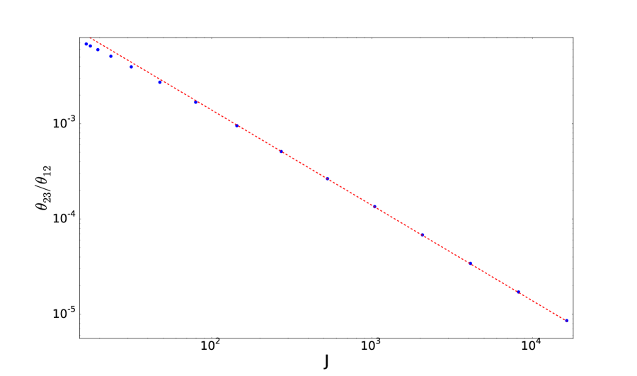
Figure 4: $\theta_{23}/\theta_{12}$ for the example in figure 3. This ratio appears to decrease like $J^{-1}$.

A more general, rotationally invariant equation is

$$\theta=\langle\alpha|~{}\Theta~{}|\alpha\rangle~{}~{},~{}~{}~{}\mathrm{where}~{}\Theta:=\sqrt{-\sum_{i\neq j}[X_{i},X_{j}]^{2}}~{}.$$ (88)

We have introduced a new operator, $\Theta$, which will play an important role in the next section.

Equation (86) has a simple geometric interpretation: the local noncommutativity on the round sphere is constant and equal to $1/J$. A single noncommutative ‘cell’ with this area is mapped to an ellipse with area $(\det\,\boldsymbol{C})/J$, which is just the noncommutativity in equation (86). In other words, the local noncommutativity is the volume form on the emergent surface divided by the volume form on the sphere, times $J^{-1}$.

The local noncommutativity is not constant on the surface. An explicit computation on the ellipsoid in equation (27) shows that its derivatives are

$$\frac{\partial\theta}{\partial x} =\frac{b(c_{1}c_{3}+c_{2}c_{4})-a(c_{3}^{2}+c_{4}^{2})}{(c_{1}c_{4}-c_{2}c_{3})J}~{}~{}~{}\mathrm{and}$$ (89)

$$\frac{\partial\theta}{\partial y} =\frac{a(c_{1}c_{3}+c_{2}c_{4})-b(c_{1}^{2}+c_{2}^{2})}{(c_{1}c_{4}-c_{2}c_{3})J}~{}.$$ (90)

If we include higher order polynomials, the appropriate coefficients in $p_{1}^{(2)}$ and $p_{2}^{(2)}$ enter in the same way as $a$ and $b$ above. Thus, we see that having these coefficients larger makes the noncommutativity vary faster, as we have mentioned before.

3.7 Coherent states overlaps, U(1) connection and $F_{\mu\nu}$ on a D2-brane

Since coherent states are associated with points, it is important that the overlap between coherent states corresponding to well-separated points be small.

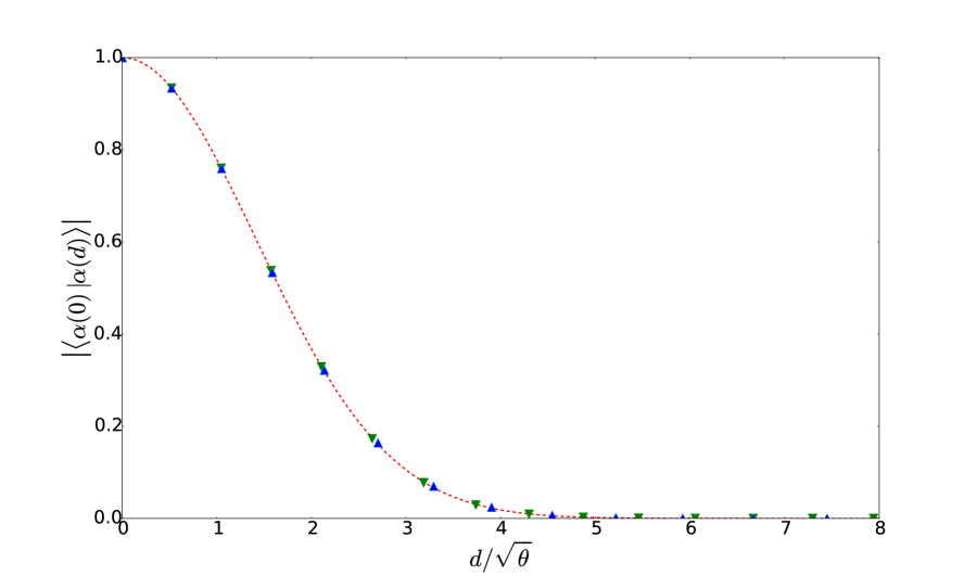
Figure 5: Magnitude of the overlap between the eigenstate corresponding to the point p at the north pole and the eigenstate corresponding to a point p’ a distance $|d|$ away. The green $\blacktriangledown$ corresponds to points p’ with $x_{2}=0$, while the blue $\blacktriangle$ corresponds to p’ with $x_{1}=0$. The dashed line corresponds to equation (93). Plotted for an ellipsoid with $c_{1}$=1, $c_{2}$=0.75, $c$=12, with $N$=16,384.

Consider two points p and p^′ on the emergent surface which are within a distance of order $1/\sqrt{N}$ of each other. For large $N$, the coefficients $c_{i}$, $a$, $b$, $c$ etc$\ldots$ that locally characterize the surface are approximately the same. However, the corresponding pre-images of p and p^′ on the unit sphere in $w$-space are sufficiently far apart that the basis in which equation (32) is written is completely different. Therefore, the approximate coherent state at the point p^′ can be obtained from the coherent state at the point p by an SU(2) rotation (in the $N$-dimensional representation). Explicitly,

$$|\alpha^{\prime}\rangle=e^{i(-D_{2}L_{1}+D_{1}L_{2})}~{}|\alpha\rangle~{},$$ (91)

where $D_{1}$ and $D_{2}$ are small displacements in $w$-space corresponding to moving from p to p^′. Since we have positioned p at the north pole of the unit sphere, there is no displacement in the 3-direction. $L_{1}$ and $L_{2}$ can be written in terms of $A$ and $A^{\dagger}$ via equation (29), and we get that

$$|\alpha^{\prime}\rangle=e^{\frac{i}{2\theta}(dA+\bar{d}A^{\dagger})}~{}|\alpha\rangle~{},$$ (92)

where $d=x^{\prime}_{2}-ix^{\prime}_{1}$, with $x^{\prime}_{1}$, $x^{\prime}_{2}$ being the coordinates of point p^′. To compute the overlap between $|\alpha\rangle$ and $|\alpha^{\prime}\rangle$, we use the Baker-Campbell-Hausdorff formula to leading order, together with $A|\alpha\rangle\approx 0$:

$$\langle\alpha|\alpha^{\prime}\rangle~{}=~{}\langle\alpha|~{}e^{-\frac{1}{8\theta^{2}}d\bar{d}[A,A^{\dagger}]}~{}|\alpha\rangle~{}\approx~{}e^{-\frac{|d|^{2}}{4\theta}}~{},$$ (93)

since $[A,A^{\dagger}]=2\theta(L_{3}/J)$. As can be seen in figure 5, the actual coherent states have exactly this expected behaviour.

Further, we can look at the connection defined (to within a factor of 2) in equation (28) of [1],

$$2v^{i}A_{i}=-iv^{i}\langle\alpha(x_{i})|\partial_{i}|\alpha(x_{i})\rangle~{},$$ (94)

where $v^{i}$ is a tangent vector on the emergent surface. To evaluate it, we rewrite equation (92) in terms of the small displacements $x_{1}$ and $x_{2}$:

$$|\alpha^{\prime}\rangle=e^{\frac{i}{\theta}(-x_{2}X_{1}+x_{1}X_{2})}~{}|\alpha\rangle~{}.$$ (95)

Thus, the connection is just $(A_{1},A_{2})=(-x_{1}/2\theta,x_{2}/2\theta)$ and the curvature is $F_{12}=\theta^{-1}$. This is exactly the expected result on an emergent D2-brane [11].

3.8 Nonpolynomial surfaces

Not surprisingly, our general conclusions are applicable even when the maps from the sphere to the surface of interest are not polynomial. As long as the maps are smooth enough to be approximated by a Taylor polynomial, the large $N$ limit behaviours should be similar. Examples with many desired properties can be relatively easily ‘cooked up’. Here we consider two of conceptual relevance.

Our first example using a non-polynomial map is designed to probe into the role of the parameter $\xi$. To this end, we examine

$$x_{1} =w_{3}w_{1}+\sqrt{1-w_{3}^{2}}~{}w_{2}~{},$$ (96)

$$x_{2} =-\sqrt{1-w_{3}^{2}}~{}w_{1}+w_{3}w_{2}~{}.$$ (97)

$$x_{3} =w_{3}~{}.$$ (98)

This example is designed produce a round sphere with a constant local noncommutativity $\theta$ by ‘shearing’ the original sphere (to preserve the volume form). We have checked explicitly that $\theta$ is constant over the surface and equal to $1/J$ in the large $N$ limit. The parameter $\xi$, however, is not constant, instead, we have $\xi=-i\sin(\phi)/(2-i\sin(\phi))$. This shows that $\xi$ does not play a role in the large $N$ limit of the surface: it can be changed by applying a volume preserving automorphism to the sphere. Another way to look at it is that the three matrices $X_{i}$ defined by equations (96)-(98) can be obtained from $L_{i}/J$ by a conjugation (up to some ordering ambiguities). $\xi$ can thus be viewed as a basis-dependent quantity.

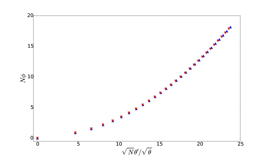
Figure 6: Angle $\phi$ between the normal vector $\vec{n}$ computed using equation (8) and the noncommutativity vector $\epsilon_{ijk}\theta_{jk}$, for the surface in equation (99) at a point given by $x=0.5$, $y=0$. The blue $\blacktriangle$ corresponds to N=3000 and the red $\blacktriangledown$ to N=12 000; the agreement between plots at different $N$ shows that the plotted quantities scale with $N$ in the expected way. On the horizontal axis we have a derivative of the noncommutativity along the surface scaled by $\sqrt{\theta}$, which increases as $\mu$ is increased in equation (99).

Another interesting example is given by

$$x_{1} =\frac{w_{1}}{\sqrt{w_{1}^{2}+w_{2}^{2}+\mu^{2}w_{3}^{2}}}~{},$$

$$x_{2} =\frac{w_{2}}{\sqrt{w_{1}^{2}+w_{2}^{2}+\mu^{2}w_{3}^{2}}}~{},$$ (99)

$$x_{3} =\frac{\mu w_{3}}{\sqrt{w_{1}^{2}+w_{2}^{2}+\mu^{2}w_{3}^{2}}}~{}.$$

In this example, we again get a round sphere, but the local noncommutativity is no longer constant. As we would expect, the actual surface at finite $N$ differs from a round sphere at order $1/N$; this corresponds to the normal vector deviating from the radial direction at the same order, as given by equation (67). Further, we can compute the noncommutativity vector $\epsilon_{ijk}\theta_{jk}$. Our assertion is that these two vectors should be nearly parallel. Figure 6 shows that, indeed, the angle between these two vectors decreases as $1/N$. This angle increases as the coefficient $\mu$ is increased, resulting in a more rapidly changing noncommutativity. Interestingly, $A_{p}$ turns out to be subleading, of order $1/N^{3/2}$ or smaller, instead of $1/N^{1/2}$, implying that $|\Delta\alpha\rangle$ is nearly parallel to $|\beta\rangle$.

The two examples in this subsection demonstrate that our approach works for surfaces which are not given by polynomial maps from the sphere. This is not surprising, as our approach should work for any surface which can be locally approximated by a polynomial map over the sphere. Relaxing the polynomial condition allows for just about any smooth surface which is topologically equivalent to a sphere to be studied with our approach.

4 Large $N$ limit and the Poisson bracket

In the previous section, we have provided a series of examples increasing in generality and all sharing the following common features: there existed a family of matrix triplets $X_{i}$ labeled by their size $N$. Each such triplet give rise to a surface $\mathcal{S}_{N}$ given by the locus of points where $H_{\mathrm{eff}}(x_{i})$ had a zero eigenvalue. The zero eigenvector of $H_{\mathrm{eff}}$ at a point on a surface such that the normal to this surface was pointing in the $x_{3}$ direction was, either exactly or approximately, of the form

$$\left[\begin{array}[]{c}|\alpha\rangle\\ \hline\cr 0\end{array}\right]~{}.$$ (100)

Where the zero eigenvector was not exactly of this form, the corrections were small, of order $N^{-1/2}$.

More generally, since a rotation of the coordinate system can be effected by an SU(2) rotation of the $\sigma_{i}$ matrices in $H_{\mathrm{eff}}$, the zero eigenvector at an arbitrary point $p$ has the form

$$|\Lambda_{p}\rangle~{}=~{}\left[\begin{array}[]{c}|\alpha_{1}\rangle\\ \hline\cr|\alpha_{2}\rangle\end{array}\right]~{}=~{}\left[\begin{array}[]{c}a|\alpha_{p}\rangle\\ \hline\cr b|\alpha_{p}\rangle\end{array}\right]~{}+~{}{\cal{O}}\left(N^{-1/2}\right)$$ (101)

where $|a|^{2}+|b|^{2}=1$ and where $|\alpha_{p}\rangle$ is a unit $N$-dimensional vector.

Given the two parts of a zero eigenvector of $H_{\mathrm{eff}}$, $|\alpha_{1}\rangle$ and $|\alpha_{2}\rangle$, at finite $N$, we compute $|\alpha_{p}\rangle$ as follows: find the normal vector to the surface, $n_{i}=\langle\Lambda_{p}|\sigma_{i}|\Lambda_{p}\rangle$. Then, find the SU(2) rotation that brings this vector to point in the positive $x_{3}$ direction and apply it to $\Lambda_{p}$. Then, the top component of of $|\Lambda_{p}\rangle$ is $|\alpha_{p}\rangle$. Explicitly,

$$|\alpha_{p}\rangle~{}~{}=~{}~{}\cos(\theta_{\hat{n}}/2)e^{i\phi_{\hat{n}}/2}|\alpha_{1}\rangle~{}+~{}\sin(\theta_{\hat{n}}/2)e^{-i\phi_{\hat{n}}/2}|\alpha_{2}\rangle~{},$$ (102)

where $\theta_{\hat{n}}$ and $\phi_{\hat{n}}$ are the polar angles of the unit normal vector $\hat{n}$.

Once the coherent state $|\alpha_{p}\rangle$ corresponding to a point is identified, we can define a correspondence between functions on the large-N surface $f$ and operators ($N\times N$ matrices) $M_{f}$ through

$$f(\tau)=\langle\alpha_{p}|M_{f}|\alpha_{p}\rangle~{},$$ (103)

where $\tau=(\tau_{1},\tau_{2})$ is a coordinate of some point $p$ on the surface.

The function $s:M_{f}\rightarrow f$ is usually called the symbol map; using a coherent state to define the symbol is an approach due to Berezin [9]. The implied noncommutative star product is

$$(f\star g)(\tau):=\langle\alpha_{p}|M_{f}\,M_{g}|\alpha_{p}\rangle~{}.$$ (104)

The star product is not unique, ie it is not fixed by the surface and the noncommutativity parameter $\theta$ alone. There are many different triplets of matrices that give the same surface and noncommutativity; different triplets would lead to different star products. Only the leading order of the commutator $f\star g-g\star f\approx\theta$ is universal. For example, the details of the star product depend on $\xi$ which we know to be arbitrary. However, the star product implies, in the large $N$ limit, a unique antisymmetric bracket,

$$\{f,g\}:=N\left(f\star g-g\star f\right)~{}.$$ (105)

We would like this bracket to give us a Poisson structure on our emergent surface. It is naturally skew-symmetric and satisfies the Jacobi identity, so it is a Lie bracket. To be a Poisson bracket, it also needs to satisfy the Leibniz Rule:

$$\{fg,h\}=f\{g,h\}+g\{f,h\}~{}.$$ (106)

(Notice that these are ordinary multiplications now, not star-products.)

Instead of directly proving that the Leibniz Rule holds, we will show that our definition of a star product is equivalent to

$$\{f,g\}=\frac{1}{\rho}\epsilon^{ab}\,\partial_{a}f\,\partial_{b}g$$ (107)

for some function $\rho$ on the surface. In particular, we will have

$$\rho=\frac{\sqrt{\det g}}{N\theta}~{},$$ (108)

where $g$ is the pullback metric on the noncommutative surface and $\theta$ is the local noncommutativity parameter defined in subsection 3.6.

Let’s follow our previous approach, and consider not only $X_{i}$ to be polynomials in $L_{1}/J$, $L_{2}/J$ and $L_{3}/J-1$, but also consider operators that are polynomials in $X_{i}$ (and therefore polynomials in $L_{1}/J$, $L_{2}/J$ and $L_{3}/J-1$). The degrees and coefficients of all the polynomials are fixed while $N\rightarrow\infty$. First, consider the expectation value $\langle\alpha_{p}|\,M\,|\alpha_{p}\rangle$ of some such operator $M=m(X_{1},X_{2},X_{3})$ in a coherent state, where $m(\cdot,\cdot,\cdot)$ is a polynomial function. We can compute $\langle\alpha_{p}|\,M\,|\alpha_{p}\rangle$ at a point $p$ where the normal points straight up by first writing $M$ as a polynomial in $L_{1}/J$, $L_{2}/J$, and $(L_{3}-1)/J$. Then, from equations (81), (82) and (83), we see that the leading order piece (which stays finite as $N\rightarrow\infty$) is simply the constant term. Thus,

$$\langle\alpha_{p}|\,M\,|\alpha_{p}\rangle=m(y_{1},y_{2},y_{3})~{},$$ (109)

where $y_{i}$ are the coordinates of the surface at point $p$ as defined in equations (25).

Now that we have shown that the expectation value in a coherent state at a point of any polynomial (in $X_{i}$) operator is exactly what we would expect, let’s think about the expectation value of the commutator of two such operators $M_{1}$ and $M_{2}$. Consider then two polynomials, $m_{1}$ and $m_{2}$ in $x_{1}$, $x_{2}$ and $x_{3}$, and the corresponding operators $M_{1}=m_{1}(X_{1},X_{2},X_{3})$ and $M_{2}=m_{2}(X_{1},X_{2},X_{3})$. We have already argued that $\theta_{12}$ is much larger than $\theta_{13}$ and $\theta_{23}$. A similar argument extended to functions of $X_{i}$ shows that, as long as $X_{i}$s are of the form (25), we have

$$\langle\alpha_{p}|\,-i[M_{1},M_{2}]\,|\alpha_{p}\rangle~{}=~{}\theta_{12}\left(\frac{\partial m_{1}(y_{1},y_{2},y_{3})}{\partial y_{1}}\frac{\partial m_{2}(y_{1},y_{2},y_{3})}{\partial y_{2}}-\frac{\partial m_{1}(y_{1},y_{2},y_{3})}{\partial y_{2}}\frac{\partial m_{2}(y_{1},y_{2},y_{3})}{\partial y_{1}}\right)~{}.$$ (110)

Thus, for the two functions on the noncommutative surface given as restrictions of the polynomials $m_{a}$: $f_{a}(\sigma)=m_{a}(x_{i}(\sigma))$, the bracket is

$$\{f_{1},f_{2}\} =N\langle\alpha_{p}|\,[M_{1},M_{2}]\,|\alpha_{p}\rangle$$ (111)

$$=N\theta~{}\left(\frac{\partial\sigma_{a}}{\partial x_{1}}\frac{\partial\sigma_{b}}{\partial x_{2}}-\frac{\partial\sigma_{a}}{\partial x_{2}}\frac{\partial\sigma_{b}}{\partial x_{1}}\right)\frac{\partial f_{1}}{\partial\sigma_{a}}\frac{\partial f_{2}}{\partial\sigma_{b}}=N\theta~{}\frac{\epsilon_{ab}}{\sqrt{\det g}}\frac{\partial f_{1}}{\partial\sigma_{a}}\frac{\partial f_{2}}{\partial\sigma_{b}}~{},$$

in agreement with equations (107) and (108).

To summarize, we have proven that our emergent surface is equipped with natural Poisson bracket which satisfies the correspondence principle

$$\{\cdot,\cdot\}~{}~{}\leftrightarrow~{}~{}-iN[\cdot,\cdot]~{}.$$ (112)

Essential for our argument to work was the noncommutativity vector $\epsilon_{ijk}\theta_{jk}$ being nearly parallel to the normal vector $n_{i}$, as shown in Figure 6. If this was not the case, the bracket we defined would fail to be a Poisson bracket.

For the remainder of this section, we will answer the following question: given a surface embedded in three dimensions and a Poisson structure on this surface, does there exist a matrix description that approximates this surface?

Our construction gives a positive answer to this question, and provides restrictions on the surface and on $N\theta$ for the approximation to be good. We focus on $N\theta$ (rather than $\theta$ itself) as this is a finite quantity in the large $N$ limit and determines the Poisson structure through equation (108). Given a surface and a function $N\theta$ on this surface, we can always define a map from the unit sphere to this surface such that the ratio of the volume form on the surface to the volume form on the sphere is $N\theta$ (see equation (26)). In fact, we can find many such functions. Which we pick will affect $\xi$ and the higher orders of the star product, but not the overall noncommutative structure. Note, however, that it is not possible to set $\xi$ to zero everywhere for a generic noncommutative surface. $\xi$ is zero if the metric on the emergent surface is proportional to the metric on the sphere, while the coefficient of this proportionality must be the noncommutativity $\theta$, which is fixed. These two requirements would fix (up to diffeomormisms) the metric on the emergent surface, which is already fixed by the embedding. To view this in a different way, the freedom in choosing a map from the sphere to the emergent surface is the freedom to pick two functions on the sphere. One of these functions is fixed by requiring a particular noncommutativity $\theta$. The remaining function can be used to change $\xi$. However, $\xi$ is a complex function, so requiring it to vanish over-constrains the problem.

Given a map from the sphere to the desired surface, we need only replace the rectilinear coordinates on the sphere with some SU(2) generators $L_{i}$ and we obtain a triplet of matrices $X_{i}$ which lead us to the appropriate noncommutative structure. Here, again, there is ambiguity in the ordering of the operators. Its effects are suppressed by powers of $1/N$ and it affects higher order terms in the star product (but not the leading order term).

For this construction to work, the surface we start with must be sufficiently smooth. Alternatively, we could say that we need to pick an irrep of SU(2) large enough to accommodate a rapidly varying surface. Two conditions seem necessary: that the curvature radii of the surface at any point be much larger than the diameter of a noncommutative ‘cell’ ($R_{\mathrm{curvature}}\gg\sqrt{\theta}~{}\sim~{}N^{-1/2}$) and that $\theta$ change slowly. Let $\theta^{\prime}$ be a derivative of $\theta$ in some tangent direction. Then, the change in noncommutativity over a single cell (which has an approximate diameter of $\sqrt{\theta}$), $\sqrt{\theta}\theta^{\prime}$, should be be small when compared with $\theta$ itself: $\theta^{\prime}/\sqrt{\theta}\ll 1$ ($\theta^{\prime}/\sqrt{\theta}\sim N^{-1/2}$). As we have already discussed, in equation (70)—which was was the basis for our perturbative definition of a general surface near some point—the coefficients in the two diagonal terms (such as $c$) control the curvature of the surface while the coefficients of the off-diagonal terms (such as $a$ and $b$) control $\theta^{\prime}/\theta$ (see equations (89) and (90)). Further, as we have discussed, large ‘curvature coefficients’ lead to large $|\beta\rangle$ while large ‘theta variability coefficients’ lead to large $|\Delta\alpha\rangle$. The larger these coefficients are, the larger $N$ must be to compensate, or higher order terms would spoil the correspondence with the classical limit we have built up. Generally speaking, the factorization of eigenstate property in equation (101) fails when curvatures are too large at a given $N$ (since $|\beta\rangle$ becomes large). On the other hand, when the noncommutativity varies too quickly, the Poisson brackets involving it (such as $\{N\theta,f\}$) will turn out to be too large.

5 Area and minimal area surfaces

In equation (88), we introduced an operator whose expectation value in a coherent state is the local noncommutativity $\theta$. The noncommutativity $\theta$ has units of length-squared, and it can be interpreted as the area of a single noncommutative ‘cell’. This is similar to thinking of phase space as made up of elementary cells whose area is $\hbar$. In string theory, where a noncommutative surface is made up of lower dimensional D-branes ‘dissolved’ in the surface, we can think of $\theta$ as the area occupied by a single D-brane, or, equivalently, the inverse of the D-brane density. If we divide the surface into $N$ noncommutative cells, adding up the areas of all these cells we should get the total area of the surface. This is in fact borne out here, as the operator $\Theta$ introduced in equation (88) has a second role: its trace seems to correspond to the area of the surface

$$A=2\pi~{}\mathrm{Tr}~{}\Theta=2\pi~{}\mathrm{Tr}~{}\sqrt{-\sum_{i,j}[X_{i},X_{j}]^{2}}~{}.$$ (113)

Numerical evidence that this formula holds in is shown in figure 7.

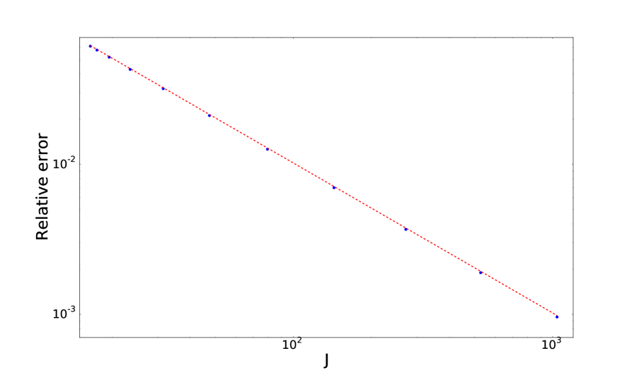
Figure 7: Relative error in the noncommutative area as given in equation (113) compared to the classical area, for an ellipsoid with major axes 6, 3 and 1. The error falls off with $J$ like $J^{-1}$; a best fit line, $1.02/J$, is shown to guide the eye.

Consider now minimal area surfaces. If we parametrize our emergent surface with coordinates $\sigma_{a}$ and define the pullback metric on this surface:

$$g_{ab}=\sum_{i=1}^{3}~{}\frac{\partial x_{i}}{\partial\sigma_{a}}~{}\frac{\partial x_{i}}{\partial\sigma_{b}}~{},$$ (114)

(locally) minimal surfaces are solutions to the equations

$$\Delta x_{k}(\sigma_{a})=0~{},~{}~{}~{}k=1\ldots 3~{},$$ (115)

where the Laplacian is, as usual

$$\Delta=\frac{1}{\sqrt{g}}~{}\frac{\partial}{\partial\sigma_{a}}~{}\sqrt{g}g^{ab}~{}\frac{\partial}{\partial\sigma_{b}}~{},$$ (116)

and where $g$ is the determinant of the metric $g_{ab}$.

It is easy to check that these minimal surface equations can be written in terms of the Poisson bracket (107) as

$$\sum_{i=1}^{3}\{x_{i},\{x_{i},x_{k}\}\}-\frac{1}{2}\sum_{i=1}^{3}~{}\frac{\rho^{2}}{g}\left\{x_{i},\frac{g}{\rho^{2}}\right\}\{x_{i},x_{k}\}=0~{}.$$ (117)

Let’s now rewrite this equation in terms of $\theta$ (using equation (108)):

$$\sum_{i=1}^{3}\{x_{i},\{x_{i},x_{k}\}\}-\frac{1}{2}\sum_{i=1}^{3}~{}\theta^{-2}\left\{x_{i},\theta^{2}\right\}\{x_{i},x_{k}\} =$$ (118)

$$\sum_{i=1}^{3}\{x_{i},\{x_{i},x_{k}\}\}+\sum_{i=1}^{3}~{}\theta\left\{x_{i},\theta^{-1}\right\}\{x_{i},x_{k}\} = 0~{},$$

or, in a more suggestive form (removing an overall factor of $\theta$),

$$\sum_{i=1}^{3}\{x_{i},\theta^{-1}\{x_{i},x_{k}\}\}=0~{}.$$ (119)

This should be compared with the variation of our expression for the area of the noncommutative surface (113):

$$\frac{\partial A}{\partial X_{1}}~{}=~{}\frac{1}{2}\left(~{}\left[X_{2},{\Theta}^{-1}[X_{2},X_{1}]+[X_{2},X_{1}]{\Theta}^{-1}\right]~{}+~{}(2\rightarrow 3)~{}\right)~{}=~{}0~{}.$$ (120)

Taking an expectation value of equation (120) w.r.t. a coherent state, we obtain equation (119), confirming that the area of the noncommutative surface is indeed given by equation (113).

Notice that this equation differs from that for a static configuration in a generic matrix model (such as BFSS or IKKT), which is

$$[X_{i},[X_{i},X_{k}]]=0~{}.$$ (121)

This is because the Lagrangian for these matrix models contain a term of the form $[X_{i},X_{j}]^{2}$ which is the square of our operator $\Theta$. When considering minimum area surfaces in matrix models, when the noncommutativity varies over the surface, the appropriate equation is not (121), but (120), or more generally

$$\Theta^{-1}[X_{i},[X_{i},X_{k}]]+[X_{i},[X_{i},X_{k}]]\Theta^{-1}+[X_{i},\Theta^{-1}][X_{i},X_{k}]+[X_{i},X_{k}][X_{i},\Theta^{-1}]=0~{},$$ (122)

which, in the large $N$ limit where ordering issues can be ignored, can be simplified to

$$[X_{i},[X_{i},X_{k}]]~{}+~{}\Theta[X_{i},\Theta^{-1}][X_{i},X_{k}]~{}=~{}0$$ (123)

or

$$[X_{i},[X_{i},X_{k}]]~{}-~{}\frac{1}{2}\Theta^{-2}[X_{i},\Theta^{2}][X_{i},X_{k}]~{}=~{}0~{}.$$ (124)

This last equation matches the original equation (117). It is important to notice that the second term in the above equation (124) has the same N-scaling as the first term: both are proportional to $N^{-2}$. Thus, this term cannot be neglected even in the large $N$ limit.

To gain more insight into the formula for the area of the surface, we can examine the formula for the area in terms of the Poisson bracket:

$$A=\int d^{2}\sigma\frac{\sqrt{g}}{N\theta}~{}\sqrt{\sum_{i,j}\{x^{i},x^{j}\}}~{}\rightarrow~{}\int d^{2}\sigma\frac{\sqrt{g}}{\theta}~{}\sqrt{-[X_{i},X_{j}]^{2}}~{}.$$ (125)

The formula in equation (125) is essentially the bosonic part of the Nambu-Goto action for a string worldsheet. This action is classically equivalent to the Schild action [13], whose quantization via matrix regularization gives the IKKT model [14]. Equivalence of these two actions is proven by the standard method involving an auxiliary field the inclusion of which removes the square root from the action [15] (for a review, see [16]). In the case of the correspondence between the Nambu-Goto and the Polyakov action, this auxiliary field is the worldsheet metric. Here, its role seems to be linked to the local noncommutativity $\theta$. This is not surprising: if the matrix model is to be viewed as a quantization of the surface, we should be free to pick any local noncommutativity we chose, so it can play the role of an auxiliary field. This point of view provides a physical interpretation to the quantum equivalence of the IKKT and the nonabelian Born-Infeld model.

Finally, our computation allows us to write down the noncommutative Laplacian on our emergent surface; it is, ignoring higher $1/N$-corrections

$$\Delta~{}=~{}\Theta^{-2}[X_{i},[X_{i},~{}\cdot~{}]]~{}-~{}\frac{1}{2}\Theta^{-4}[X_{i},\Theta^{2}][X_{i},~{}\cdot~{}]~{}.$$ (126)

This equation could be the starting point for a study of the effects of varying noncommutativity on noncommutative field theory.

6 The torus

Our construction has a natural extension to a toroidal surface embedded in flat three space. Just as surfaces topologically equivalent to a sphere were build by considering maps from the noncommutative sphere algebra, to make a torus we use maps from the appropriate algebra.

Consider a surface given by

$$x_{1} =(R+r\cos u)\cos v~{},$$ (127)

$$x_{2} =(R+r\cos u)\sin v~{},$$ (128)

$$x_{3} =r\sin u~{},$$ (129)

where $u,v\in[0,2\pi]$ and $r<R$. Now, consider the standard clock-and-shift matrices $U$ and $V$ that are usually used to define the noncommutative two-torus:

$$UV =e^{2\pi i/N}VU~{},$$ (130)

$$U_{kl} =\delta_{kl}e^{2\pi i(k/N)}~{},$$ (131)

$$V_{kl} =\delta_{k_{\mathrm{mod}N},(l+1)_{\mathrm{mod}N}}~{}.$$ (132)

In the noncommutative torus, operators of the form $U^{n}V^{m}$ are associated with functions on the torus of the form $e^{inu}e^{inv}$. To define the noncommutative torus embedded in $\mathbb{R}^{3}$ we thus simply substitute $e^{iu}\rightarrow U$ and $e^{iv}\rightarrow V$ in equations (127)-(129), symmetrizing when necessary to obtain hermitian matrices. Numerical analysis shows that the resulting toroidal surface is smooth and has the appropriate large $N$ limit (with $A_{p}$ decreasing for large $N$ as $N^{-1/2}$, the surface approaching the classical shape and the area of the surface well approximated by equation (113)).

Once we have obtained this particular toroidal surface, any other surface with this topology (including surfaces with the same shape but different local noncommutativity, for example uniform one) can be obtained by smooth maps in a way that parallels our discussion of spherical surfaces. It would be interesting to consider a deformation which connects the torus and the sphere and to examine what happens at the point of topological transition in detail.

7 Open questions and future work

There are many questions which our work does not address.

For example, one can ask if equation (113) can be proven analytically, starting with the definition of the surface from $H_{\mathrm{eff}}$. A reasonable start for such a proof might be equation (125). If we assume that

$$\frac{1}{N}~{}\mathrm{Tr}~{}~{}\cdot~{}=~{}\frac{1}{2\pi}\int d^{2}\sigma\frac{\sqrt{g}}{N\theta}~{}\langle\alpha(\sigma)|~{}~{}\cdot~{}~{}|\alpha(\sigma)\rangle~{},$$ (133)

we recover equation (113). Equation (133) is equivalent to

$$\frac{1}{2\pi}\int d^{2}\sigma\frac{\sqrt{g}}{\theta}~{}|\alpha(\sigma)\rangle\langle\alpha(\sigma)|~{}=~{}\boldsymbol{1}_{N}~{}.$$ (134)

Above equation implies a relationship between the trace and the integral of the noncommutative surface

$$\frac{1}{N}~{}\mathrm{Tr}~{}~{}\leftrightarrow~{}~{}\frac{1}{2\pi}\int d^{2}\sigma\frac{\sqrt{g}}{N\theta}~{}.$$ (135)

A completeness relationship such as (134) is necessary for the symbol map from operators to functions on the emergent surface to have a unique inverse, which in turn is necessary for the definition of the star product to make sense. In principle, it should be possible to prove such a completeness relationship starting with equation (1).

In subsection 3.7, we briefly addressed the question of the U(1) connection on the emergent D2-brane. Extending this approach should allow us to prove the equivalence of the nonabelian effective action for D0-branes and the abelian effective action for a D2-brane. More simply, it should be possible to show the equivalence of the BPS conditions in these two scenarios.

It would be interesting to see how our set up could be extended to surfaces which are not topologically equivalent to a sphere or a torus. It should be possible, for example, to find matrix triplets $X_{i}$ which correspond to emergent surfaces with a larger number of handles—and for which the large $N$ limit we describe holds. One could check, for example, whether the noncommutative surfaces given in [8] have a large $N$ limit in the sense in which we define it here. Further, it would be interesting to see how our toroidal construction in section 6 is related to that in [8].

Finally, there are many generalizations of equation (1) that would be interesting to explore, including generalizations to higher dimensions (both of the embedding space and the emergent surface) and those to curved embedding space. One could also consider Lorentzian signature models, which would be useful in the context of recent progress in cosmology arising from matrix models, as in [17].

References

- [1] D. Berenstein and E. Dzienkowski, Matrix embeddings on flat and the geometry of membranes, Phys.Rev. D86 (2012) 086001, [arXiv:1204.2788].
- [2] R. C. Myers, Dielectric branes, JHEP 9912 (1999) 022, [hep-th/9910053].
- [3] I. Ellwood, Relating branes and matrices, JHEP 0508 (2005) 078, [hep-th/0501086].
- [4] H. Steinacker, Non-commutative geometry and matrix models, PoS QGQGS2011 (2011) 004, [arXiv:1109.5521].
- [5] H. Steinacker, Emergent Geometry and Gravity from Matrix Models: an Introduction, Class.Quant.Grav. 27 (2010) 133001, [arXiv:1003.4134].
- [6] M. Kontsevich, Deformation quantization of poisson manifolds, Letters in Mathematical Physics 66 (2003), no. 3 157–216, [q-alg/9709040].
- [7] J. Arnlind, M. Bordemann, L. Hofer, J. Hoppe, and H. Shimada, Fuzzy Riemann surfaces, JHEP 0906 (2009) 047, [hep-th/0602290].
- [8] J. Arnlind, M. Bordemann, L. Hofer, J. Hoppe, and H. Shimada, Noncommutative Riemann Surfaces, ArXiv e-prints (Nov., 2007) [arXiv:0711.2588].
- [9] F. Berezin, General Concept of Quantization, Commun.Math.Phys. 40 (1975) 153–174.
- [10] G. Ishiki, Matrix Geometry and Coherent States, arXiv:1503.01230.
- [11] N. Seiberg and E. Witten, String theory and noncommutative geometry, JHEP 9909 (1999) 032, [hep-th/9908142].
- [12] J. Arnlind and J. Hoppe, The world as quantized minimal surfaces, Phys.Lett. B723 (2013) 397–400, [arXiv:1211.1202].
- [13] A. Schild, Classical Null Strings, Phys.Rev. D16 (1977) 1722.
- [14] N. Ishibashi, H. Kawai, Y. Kitazawa, and A. Tsuchiya, A Large N reduced model as superstring, Nucl.Phys. B498 (1997) 467–491, [hep-th/9612115].
- [15] A. Fayyazuddin, Y. Makeenko, P. Olesen, D. J. Smith, and K. Zarembo, Towards a nonperturbative formulation of IIB superstrings by matrix models, Nucl.Phys. B499 (1997) 159–182, [hep-th/9703038].
- [16] K. Zarembo and Y. Makeenko, An introduction to matrix superstring models, Phys.Usp. 41 (1998) 1–23.
- [17] S.-W. Kim, J. Nishimura, and A. Tsuchiya, Expanding (3+1)-dimensional universe from a Lorentzian matrix model for superstring theory in (9+1)-dimensions, Phys.Rev.Lett. 108 (2012) 011601, [arXiv:1108.1540].