From an array of quantum wires to three-dimensional fractional topological insulators

Abstract

The coupled-wires approach has been shown to be useful in describing two-dimensional strongly interacting topological phases. In this manuscript we extend this approach to three-dimensions, and construct a model for a fractional strong topological insulator. This topologically ordered phase has an exotic gapless state on the surface, called a fractional Dirac liquid, which cannot be described by the Dirac theory of free fermions. Like in non-interacting strong topological insulators, the surface is protected by the presence of time-reversal symmetry and charge conservation. We show that upon breaking these symmetries, the gapped fractional Dirac liquid presents unique features. In particular, the gapped phase that results from breaking time-reversal symmetry has a halved fractional Hall conductance of the form $\sigma_{xy}=\frac{1}{2}\frac{e^{2}}{mh}$ if the filling is $\nu=1/m$. On the other hand, if the surface is gapped by proximity coupling to an $s$-wave superconductor, we end up with an exotic topological superconductor. To reveal the topological nature of this superconducting phase, we partition the surface into two regions: one with broken time-reversal symmetry and another coupled to a superconductor. We find a fractional Majorana mode, which cannot be described by a free Majorana theory, on the boundary between the two regions. The density of states associated with tunneling into this one-dimensional channel is proportional to $\omega^{m-1}$, in analogy to the edge of the corresponding Laughlin state.

I Introduction

The theoretical predictions and consequent experimental discoveries of topological insulators in two and three dimensions Pankratov et al. (1987); Kane and Mele (2005); Bernevig et al. (2006); König et al. (2007); Liu et al. (2012); Roth et al. (2009); Nowack et al. (2013); Knez et al. (2012); Spanton et al. (2014); Fu et al. (2007); Fu and Kane (2007); Hsieh et al. (2008) have enriched our understanding of topological phases of matter. Importantly, it was demonstrated that topological states may be much more widespread than previously believed, and that in particular they can exist beyond the realms of two-dimensions (2D). Since then, many systems realizing various topological phases have been proposed, and a periodic table for topological phases of non-interacting fermions has been established Schnyder et al. (2008); Kitaev (2009). While this classification is limited to topological states protected by time-reversal symmetry, particle-hole symmetry, and chiral symmetry, the existing tools can be applied to other protecting symmetries. A particularly notable extension of the above classification are the topological crystalline insulators Fu (2011), protected by the crystal point group symmetries.

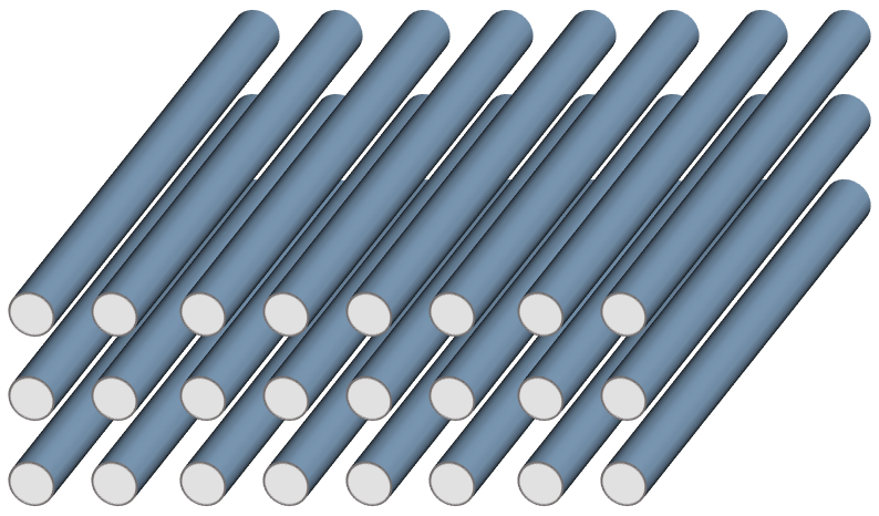
Figure 1: A schematic depiction of the array of wires studied in this manuscript. The coupled-wires approach allows us to treat interacting terms using the Abelian bosonization framework, making it very useful in constructing strongly interacting topological phases. Throughout this work, we focus on the construction of a fractional strong topological insulator.

The effects of strong interactions on topological materials, on the other hand, are much more subtle. Particularly interesting situations occur when interactions stabilize topologically ordered phases that cannot be realized in free-fermion systems. The excitations in these systems have fractional statistics, and usually carry fractional quantum numbers. Thus, topologically ordered systems are sometimes called fractional phases. The most famous example of such a phase is the fractional quantum Hall effect (FQHE).

While topological phases have conclusively been found to exist in three-dimensions (3D), fractional phases are still usually associated with 2D systems. This is a consequence of the well-known theorem stating that anyonic statistics between two point-particles cannot occur in 3D Doplicher et al. (1971, 1974).

A possible way to go around this theorem and realize topologically ordered phases in 3D is to consider loop excitations, which can have non-trivial braiding statistics with point-particles, as well as other loops.

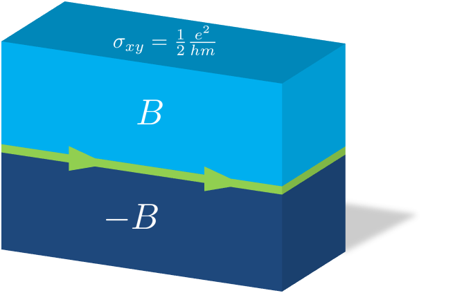
(a)

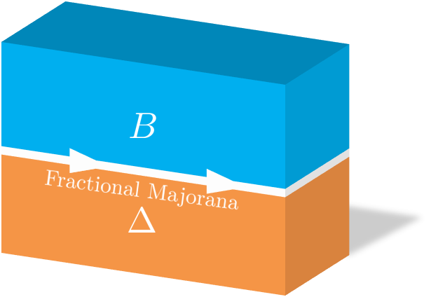
(b)

Figure 2: The fractional strong topological insulator phase we construct has an exotic fractional Dirac liquid on the surface. As in the non-interacting case, this gapless surface is protected by time reversal symmetry and charge conservation. Upon breaking any of these symmetries, we end up with a gapped surface displaying unique topological properties. For example, by breaking time-reversal symmetry, we get a halved fractional quantum Hall effect, characterized by a surface Hall conductance of the form $\sigma_{xy}=\frac{1}{2}\frac{e^{2}}{mh}$, where $m$ is an odd integer (in a state associated with the 2D Laughlin state at filling $\nu=1/m$). On the magnetic domain wall shown in (a), one therefore finds a chiral Luttinger liquid, similar to the edge mode of the corresponding 2D Laughlin-state. If the system is gapped by proximity to an $s$-wave superconductor (i.e., by breaking charge conservation), we get an exotic time-reversal invariant topological superconductor. It is interesting to study the boundary between a superconducting region and a magnetic region, as depicted in Fig (b). A fractional Majorana mode, which cannot be described by a free Majorana theory, is found on the interface between the two regions. The tunneling density of states associated with this 1D channel is proportional to $\omega^{m-1}$, in analogy to the edge of the corresponding Laughlin-state.

Indeed, a few recent works Maciejko et al. (2010); Hoyos et al. (2010); Levin et al. (2011); Swingle et al. (2011); Maciejko et al. (2012); Swingle (2012); Chan et al. (2013); Maciejko et al. (2014); Jian and Qi (2014) have used various non-perturbative approaches to discuss fractional topological insulators in 3D. These are the fractional counterparts of the well-studied non-interacting strong topological insulators.

In this work we construct a model for such systems from an array of weakly coupled wires, as illustrated in Fig. (1). The ability to introduce interactions, and treat them using the bosonization framework has made this approach successful in producing fractional phases in 2D Kane et al. (2002); Teo and Kane (2014); Klinovaja and Loss (2013); Neupert et al. (2014a); Sagi and Oreg (2014); Klinovaja and Tserkovnyak (2014); Meng and Sela (2014); Mross et al. (2015); Santos et al. (2015); Sagi et al. (2015); Gorohovsky et al. (2015); Meng et al. (2015). In addition to reproducing well-known FQHE states in the extremely anisotropic limit, it has been shown to be useful in producing new fractional states, which would otherwise be very hard to realize in terms of a microscopic model.

Here we show that the wires approach can be extended to 3D, and use it to construct a fractional strong topological insulator.

Since, by assumption, different wires are weakly coupled, we linearize their energy spectra around the Fermi-points, and treat inter-wire terms as perturbations within this linearized framework. Once the 1D spectra are linearized, we can fully describe the single and many body excitations using chiral bosonic fields. The only remnants of the original model are encoded in the values of the Fermi-momenta associated with the various wires (these are determined by the overall density, the spin-orbit coupling, the magnetic field, etc.). The Fermi-momenta determine, due to momentum conservation, the allowed inter-wire terms. To keep track of these terms, it proves useful to depict the Fermi-momenta diagrammatically. In 2D models, for example, we plot the Fermi-momenta as a function of an index enumerating the wires (see Figs. (9a)-(9b)). Importantly, the diagrams present the problem as a lattice model in a lower dimension. The task of calculating some topological properties of the full model is then reduced to the calculation of similar properties in the lower-dimensional non-interacting system. For example, the analysis of 2D topological insulators is reduced, in some aspects, to the analysis of a 1D topological system. Similarly, the analysis of a 3D strong topological insulator is reduced to the analysis of a 2D topological insulator. At integer fillings, this enables us to construct topological phases in two and three dimensions.

Upon varying the filling to a given fractional value, the pattern formed by the Fermi-momenta is modified, and we are forced to consider a different set of inter-wire terms, which in general need to involve multi-electron processes. At a specific set of filling factors, we find it useful to define new fields, associated with a new set of effective Fermi-momenta. The transformation to the new fields can be chosen such that the corresponding diagram is mapped onto the one describing a system at integer filling. Then, by repeating the analysis that led to the creation of the non-interacting topological phase in terms of the transformed fields, we get its fractional analog.

The resulting 3D topologically ordered phase studied here will be shown to have a novel gapless surface mode, which cannot be described by Dirac’s theory of free fermions. Throughout this work, we refer to the surface as a fractional Dirac liquid. In analogy to a strong topological insulator, the surface is protected by time reversal symmetry and charge conservation.

It is insightful to study what happens to the fractional Dirac theory once it is gapped by breaking any of these symmetries. We will see that if a time reversal breaking perturbation is introduced, the surface acquires a Hall conductance of the form $\sigma_{xy}=\frac{1}{2m}\frac{e^{2}}{h}$ in a state at filling $\nu=1/m$. This Hall conductance is half that of the associated 2D Laughlin FQH state, and we therefore refer to this effect as a halved fractional quantum Hall effect. This should be compared with the half-integer quantum Hall effect that occurs on the surface of a strong topological insulator, which corresponds to $m=1$ in our framework. As a result of the above, a magnetic domain wall of the type depicted in Fig. (2a) contains a gapless channel described by the chiral Luttinger-liquid theory, similar to the edge states of a Laughlin-state.

In addition, we will break charge conservation by proximity coupling the surface to an $s$-wave superconductor. The resulting superconducting state is found to be topologically non-trivial. On the surface of a non-interacting strong topological insulator, for example, one finds a phase that resembles a $p_{x}+ip_{y}$ superconductor, but has time reversal symmetry Fu and Kane (2008). One way to reveal the topological nature of the surface is to separate the surface into two domains: one with broken time-reversal symmetry, and another with broken charge conservation. It was shown in Ref. Fu and Kane (2008) that a chiral Majorana mode is localized near the boundary separating the two regions. Furthermore, it was shown in Ref. Neupert et al. (2014b) that this remains correct in the presence of interactions.

Repeating the same thought experiment in our fractional phase, we find a chiral self-Hermitian mode on the boundary, which cannot be described by a free Majorana theory, as illustrated in Fig. (2b). In particular, the tunneling density of states associated with this 1D channel is proportional to $\omega^{m-1}$, as opposed to the constant density of states characterizing free Majorana fermions. Throughout this paper, we refer to this mode as a fractional Majorana mode.

The structure of the paper is as follows: In Sec. II.1 we discuss the physics of fractional weak topological insulators. These are states constructed by stacking 2D fractional topological insulators Levin and Stern (2009). While these systems do not host anyonic excitations which are deconfined in the stacking direction, they possess interesting surface states, intimately related to those of the fractional strong topological insulator. Then, in Sec. III, we use an oversimplified yet intuitive model (with a modified time-reversal symmetry), derived from the surface of the fractional weak topological insulator, to describe the surface of the fractional strong topological insulator. The purpose of this discussion is to pedagogically derive the properties of the surface once it is gapped by breaking its protecting symmetries. We stress that these properties will be derived rigorously in Section IV without using the above oversimplified model.

In the sections that follow, we use a wire construction to create a fractional strong topological insulator. The analysis is done in a few stages. First, in Sec. IV.1 we review the construction of a 2D fractional topological insulator presented in Ref. Sagi and Oreg (2014). This model will be the starting point in our constructions of 3D states. In this section we also introduce the general approach and notations used throughout the rest of this work. Then, in Sec. IV.2-IV.3 we will show that by stacking copies of this 2D phase with a set of non-trivial inter-layer coupling terms, a fractional strong topological insulator can be stabilized. Finally, in Sec. IV.4, we will use the wires model to derive the properties of the resulting phase.

II Fractional weak topological insulators

II.1 Weak topological insulators

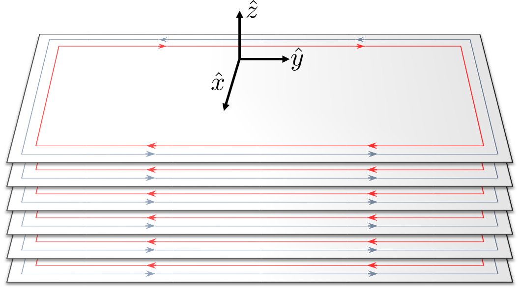
(a)

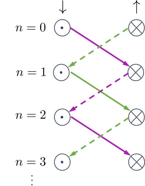
(b)

Figure 3: (a) The simplified model we use to describe a weak topological insulator. Each plane forms an $S_{z}$-conserving 2D topological insulator. The edge of each layer therefore contains counter-propagating spin-up and spin-down modes, represented by red and blue arrows. (b) A diagrammatic depiction of the surface of the simplified model. The vertical direction represents the layer index, and the horizontal direction represents spin. The symbol $\bigotimes$ ($\bigodot$) corresponds to a right (left) mover. We introduce nearest-layer coupling terms, represented by arrows connecting different chiral modes. Time reversal symmetry relates the amplitudes of the terms represented by the full arrows to the amplitudes of the terms represented by the dashed arrows. The above model can be decomposed into two decoupled gapless Hamiltonians, represented by the green and purple arrows.

Before discussing fractional weak topological insulators, we briefly review the physics of non-interacting weak topological insulators.

To construct a simple model for a weak topological insulator, we imagine stacking many 2D topological insulators (see Fig. (3a) for illustration).

For simplicity, we assume that the 2D topological insulators in the various layers conserve $S_{z}$. We can therefore describe their edge states as counter propagating spin-up and spin-down modes. In the limit where the layers are decoupled, the surface in the $xz$ direction, for example, is composed of these helical modes. The modes are represented diagrammatically in Fig. (3b), where the vertical direction represents the layer index, and the horizontal direction represents the spin. The symbol $\bigotimes$ ($\bigodot$) corresponds to a right (left) mover.

We now introduce coupling between adjacent layers. In doing so, we consider only the terms represented by the arrows in Fig. (3b), as these are the only terms capable of gapping the surface. Time reversal symmetry relates the amplitudes of the terms represented by the full arrows and those represented by the dashed arrows.

To be concrete, if we define the electron annihilation operators $\psi_{n,\uparrow}(x)$,$\psi_{n,\downarrow}(x)$ (where $n$ is the layer index), we can write the low energy surface Hamiltonian in the form

$$H=H_{z}+H_{x},$$ (1)

where

$$H_{x} =-iv\sum_{n}\int dx\left(\psi_{n,\uparrow}^{\dagger}(x)\partial_{x}\psi_{n,\uparrow}(x)\right.$$ (2)

$$\left.\hphantom{fffff}-\psi_{n,\downarrow}^{\dagger}(x)\partial_{x}\psi_{n,\downarrow}(x)\right)$$

represents the Hamiltonian of the decoupled helical edge modes, and

$$H_{z} =t\sum_{n}\int dx\left(\psi_{n,\uparrow}^{\dagger}(x)\psi_{n+1,\downarrow}(x)e^{i\alpha}\right.$$ (3)

$$\left.-\psi_{n,\downarrow}^{\dagger}(x)\psi_{n+1,\uparrow}(x)e^{-i\alpha}+h.c.\right)$$

represents their nearest-layer coupling. In the above, $\alpha$ is a fixed phase, which we set to be $0$ for simplicity.

If the system has periodic boundary conditions in the $x$ and $z$ directions, $k_{x}$ and $k_{z}$ are good quantum numbers. We can therefore write the Hamiltonian in $k$-space, where it takes the form $H=\sum_{k_{z}}\int dk_{x}\psi^{\dagger}(\vec{k})\mathcal{H}(\vec{k})\psi(\vec{k})$, with $\psi(\vec{k})=(\begin{array}[]{cc}\psi_{\uparrow}(\vec{k}),&\psi_{\downarrow}(\vec{k})\end{array})^{T}$ and

$$\mathcal{H}=-2t\sigma_{y}\sin\left(k_{z}a\right)+vk_{x}\sigma_{z}$$ (4)

(here the $\sigma_{i}$’s are Pauli matrices acting on the spin degrees of freedom). We see that we have two Dirac cones on the surface: one around $\left(k_{x}=0,k_{z}=0\right)$, and another around $\left(k_{x}=0,k_{z}=\pi\right)$. These are not protected by time-reversal symmetry, as time-reversal invariant terms can couple the two Dirac modes and gap them out. However, such terms necessarily involve a large momentum transfer. Therefore, if lattice translation invariance is also imposed, the two Dirac modes remain protected.

II.2 The surface of fractional weak topological insulators

In order to generalize the above simplified model to a fractional weak topological insulator, we imagine stacking layers of 2D fractional topological insulators. Again, we focus on the $S_{z}$ conserving case, where each 2D fractional topological insulator can be thought of as two decoupled FQHE layers. These two FQH states have equal densities, but opposite fillings $\pm\nu$ and spins.

For now, we keep the discussion general and do not provide a specific model for the 2D fractional topological insulators in the various layers. For such a concrete model, the reader is referred to Sec. IV.1, where we review the wire construction of a fractional topological insulator introduced in Ref. Sagi and Oreg (2014).

We focus on the time reversal invariant analog of a Laughlin state with filling $\nu=1/m$, where $m$ is an odd integer. Before introducing inter-layer coupling terms, the natural way to describe the edge modes of the various layers is in terms of two boson fields $\chi_{n}^{\uparrow}\text{ and }\chi_{n}^{\downarrow}$. These modes satisfy the commutation relations

$$\left[\chi_{n}^{\sigma}(x),\chi_{n^{\prime}}^{\sigma^{\prime}}(x^{\prime})\right]=\frac{1}{m}i\pi\sigma\delta_{n,n^{\prime}}\delta_{\sigma,\sigma^{\prime}}\text{{sign}}(x-x^{\prime})+\frac{1}{m^{2}}i\pi\text{{sign}}(n-n^{\prime})+\frac{1}{m^{2}}\pi\delta_{n,n^{\prime}}\sigma_{y}^{\sigma,\sigma^{\prime}},$$ (5)

where in the above $\sigma=1(-1)$ for spin $\uparrow(\downarrow)$. In terms of these, the chiral fermion operators take the form $\tilde{\psi}_{n,\sigma}\propto e^{im\chi_{n}^{\sigma}}$, and the Laughlin quasiparticle operators are given by $\tilde{\psi}_{n,\sigma}^{QP}\propto e^{i\chi_{n}^{\sigma}}$. If we introduce inter-layer coupling terms, the effective low energy Hamiltonian describing the surface is given by

$$\tilde{H}=\tilde{H}_{z}+\tilde{H}_{x},$$ (6)

where

$$\tilde{H}_{x}=\frac{mv}{4\pi}\sum_{n,\sigma}\int dx\left(\partial_{x}\chi_{n}^{\sigma}\right)^{2}$$ (7)

represents the decoupled chiral Luttinger liquids, and

$$\tilde{H}_{z} =\tilde{t}\sum_{n}\int dx\left(\tilde{\psi}_{n,\uparrow}^{\dagger}\tilde{\psi}_{n+1,\downarrow}\right.$$ (8)

$$\left.\hphantom{jmk}-\tilde{\psi}_{n,\downarrow}^{\dagger}\tilde{\psi}_{n+1,\uparrow}+h.c.\right)$$

represents their coupling. In what follows we assume that the amplitude $\tilde{t}$ is large enough such that these operators flow to the strong coupling limit (if they are considered separately). In the integer case, where $m=1$, $\tilde{H}$ reduces to the Hamiltonian $H$ defined in Eq. (1), as can be seen directly by rewriting $H$ using Abelian bosonization. In the fractional case, where $m>1$, $\tilde{H}$ cannot be mapped to a non-interacting fermionic Hamiltonian. However, the model can still be represented by the diagram shown in Fig. (3b). Notice that now the symbols $\bigotimes$ and $\bigodot$ represent right and left moving $\tilde{\psi}$ (or $\chi$) fields, respectively.

Each of the two terms in Eq. (8), if considered separately, can gap out the spectrum in the thermodynamic limit. However, the two gapped phases that result from these terms are topologically distinct. Noting that the two non-commuting operators have the same amplitude and scaling dimension, it is clear that the system must be in a critical point between the two gapped phases. We emphasize that the criticality of the surface is imposed by time reversal symmetry, and is not a result of fine-tuning the Hamiltonian. It is explicitly assumed that additional interacting terms do not destabilize the critical point. This crucial assumption must be checked for a given microscopic model.

Like in the integer case, this gapless model is represented by two decoupled gapless theories. This can be identified by writing the Hamiltonian in the form $\tilde{H}=\tilde{H}_{1}+\tilde{H}_{2},$ with

$$\tilde{H}_{1}=\frac{mv}{4\pi}\sum_{n,\sigma}\int dx\left(\partial_{x}\chi_{2n}^{\uparrow}\right)^{2}+\left(\partial_{x}\chi_{2n+1}^{\downarrow}\right)^{2}+\tilde{t}\sum_{n}\int dx\left(\tilde{\psi}_{2n,\uparrow}^{\dagger}\tilde{\psi}_{2n+1,\downarrow}-\tilde{\psi}_{2n+2,\uparrow}^{\dagger}\tilde{\psi}_{2n+1,\downarrow}+h.c.\right),$$ (9)

$$\tilde{H}_{2}=\frac{mv}{4\pi}\sum_{n,\sigma}\int dx\left(\partial_{x}\chi_{2n+1}^{\uparrow}\right)^{2}+\left(\partial_{x}\chi_{2n}^{\downarrow}\right)^{2}+\tilde{t}\sum_{n}\int dx\left(\tilde{\psi}_{2n+2,\downarrow}^{\dagger}\tilde{\psi}_{2n+1,\uparrow}-\tilde{\psi}_{2n,\downarrow}^{\dagger}\tilde{\psi}_{2n+1,\uparrow}+h.c.\right).$$ (10)

The green (purple) arrows in Fig. (3b) represent terms belonging to $\tilde{H}_{1}$ ($\tilde{H}_{2}$). In the integer case each of these Hamiltonians is described by a low energy Dirac theory, as can be seen by refermionizing the bosonic theories. Importantly, the Hamiltonians $\tilde{H}_{1}$ and $\tilde{H}_{2}$ remain gapless in the fractional case as well, as indicated by the argument we have used to show that $\tilde{H}$ is gapless. However, in the fractional case these Hamiltonians cannot be described by a low energy Dirac theory. In the future we refer to their low energy theories as fractional Dirac liquids.

III A simplified model for the surface of fractional strong topological insulators

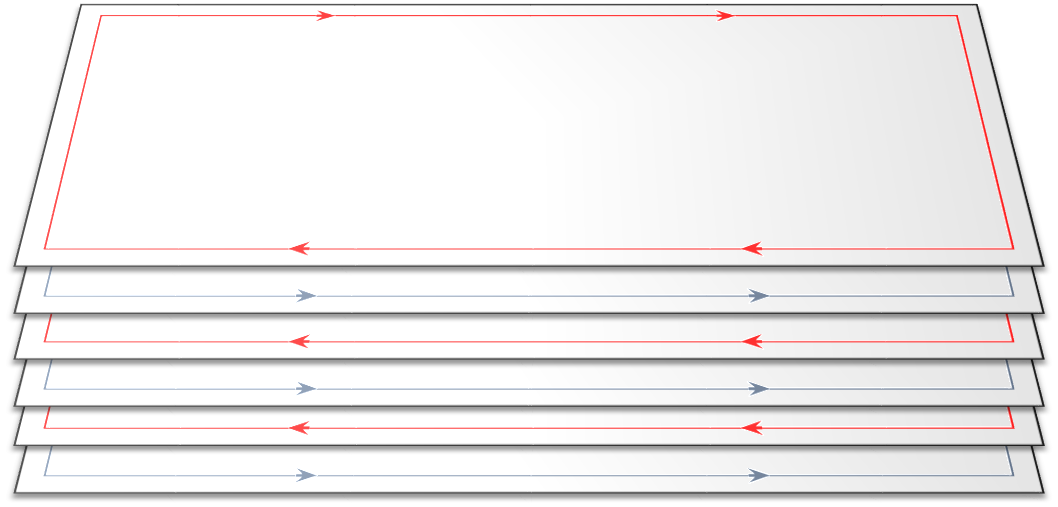
(a)

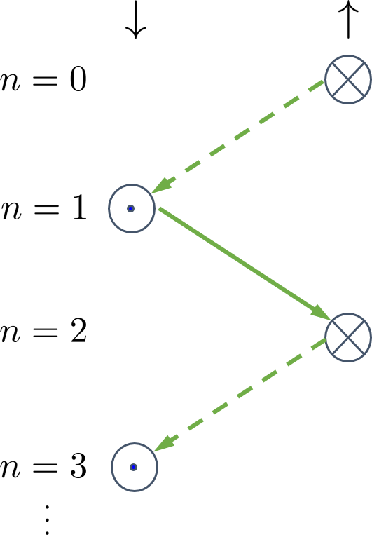
(b)

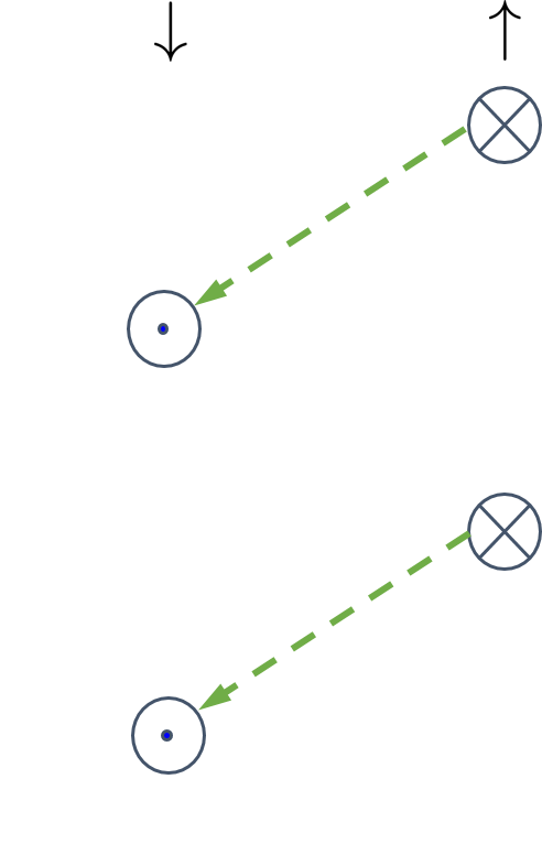
(c)

Figure 4: (a) The simplified model we use to describe an antiferromagnetic topological insulator and its fractional analog. Each layer can be thought of as a single-component QHE system at filling $\pm\nu$ (where $\nu=1$ in the integer case, and in the fractional case we consider $\nu=1/m$, where $m$ is an odd integer). Due to the existence of a modified time-reversal symmetry, given by the product of the original time-reversal operator and a translation by a unit cell, the $xz$ surface remains gapless even in the presence of inter-layer coupling terms. The surface can be described in terms of coupled 1D channels, which enables a simple derivation of universal surface properties. We argue that these properties remain true for a strong topological insulator and its fractional analog, where the surface is protected by the local time reversal symmetry. (b) A diagrammatic representation of $xz$ surface of the above model in terms of the coupled 1D chiral edge modes. (c) The diagram that corresponds to the situation where the modified time-reversal symmetry is explicitly broken by introducing a term of the form (11) with $\tilde{t}^{\prime}=\tilde{t}$.

We have seen above that the simple model for a fractional weak topological insulator can be decomposed into two decoupled gapless theories described by the Hamiltonians $\tilde{H}_{1}$ and $\tilde{H}_{2}$. In the integer case, weak topological insulators possess an even number of Dirac cones on the surface, while strong topological insulators necessarily have an odd number of Dirac cones Fu et al. (2007). By analogy, we naturally expect the low energy theory describing the surface of a fractional strong topological insulator to be related to the surface of a fractional weak topological insulator. We therefore ask whether a single decoupled surface Hamiltonian, say $\tilde{H}_{1}$, describing left movers on layers with even indices and right movers on layers with odd indices (see Fig. (4a)), can faithfully describe the surface of a fractional strong topological insulator.

Strictly speaking, this is clearly impossible since $\tilde{H}_{1}$ is not independently time reversal invariant. Nevertheless, we follow Ref. Mross et al. (2015) in noting that $\tilde{H}_{1}$ is invariant under a modified time reversal operation, defined as the product of the original time-reversal operator and a translation by a unit cell.

Such a symmetry characterizes antiferromagnetic topological insulators, which can be created, for example, by adding an antiferromagnetic order parameter to a strong topological insulator (without closing the gap). Remarkably, it was shown in Refs. Mong et al. (2010); Fang et al. (2013) that the introduction of such a time-reversal breaking perturbation does not destroy all the surface Dirac cones. Instead, the remaining Dirac cones are protected by the modified time-reversal operation described above.

This leads us to assume that $\tilde{H}_{1}$ faithfully describes the surface of the fractional analog of an antiferromagnetic topological insulator. The corresponding gapless surface is expected to be in the same universality class as the surface of a fractional strong topological insulator with a local time-reversal symmetry. We can therefore use $\tilde{H}_{1}$ to derive some of the universal properties expected to characterize the surface of a fractional strong topological insulator. Notice that the bulk excitations of the fractional antiferromagnetic topological insulator are generally different from the fractional excitations characterizing the 3D fractional strong topological insulator.

As noted in Ref. Mross et al. (2015), studying a system with the modified time-reversal symmetry, for which one can write an explicit model of the surface in terms of weakly coupled 1D channels, greatly simplifies the analysis. This is impossible in systems that have a local (unmodified) time-reversal symmetry. To study these using a set of weakly coupled 1D systems, we will be forced to explicitly construct the 3D bulk as well. This will be done in Sec. IV.

Again, we depict the surface model using diagrams representing the inter-layer terms coupling the various chiral modes. In particular, the diagram that represents the gapless surface Hamiltonian $\tilde{H}_{1}$ is shown in Fig. (4b).

Until now we have preserved the modified time-reversal symmetry and charge conservation of $\tilde{H}_{1}$, and thus the surface was found to be gapless. In what follows we focus on the properties of the surface once these protecting symmetries are explicitly broken. We will see below that the resulting gapped fractional Dirac mode has unique properties.

To break the modified time reversal symmetry, we add a perturbation of the form

$$\tilde{H}_{t} =\tilde{t}^{\prime}\sum_{n}\int dx\left(\tilde{\psi}_{2n,\uparrow}^{\dagger}\tilde{\psi}_{2n+1,\downarrow}\right.$$

$$\left.\hphantom{jmk}+\tilde{\psi}_{2n+2,\uparrow}^{\dagger}\tilde{\psi}_{2n+1,\downarrow}+h.c.\right)$$ (11)

The physics of the resulting phase becomes transparent at the points $\tilde{t}^{\prime}=\pm\tilde{t}$, where the Hamiltonian is decomposed into decoupled sine-Gordon models. For example, if $\tilde{t}^{\prime}=\tilde{t}$ the non-quadratic part of the Hamiltonian takes the form

$$2\tilde{t}^{\prime}\sum\int dx\left(\tilde{\psi}_{2n,\uparrow}^{\dagger}\tilde{\psi}_{2n+1,\downarrow}+h.c.\right)=$$

$$4\tilde{t}^{\prime}\sum\int dx\cos\left[m\left(\chi_{2n}^{\uparrow}-\chi_{2n+1}^{\downarrow}\right)\right].$$ (12)

Thus we end up with a set of mutually commuting cosine terms, which can be pinned in the ground state and fully gap the surface. This configuration is depicted diagrammatically in Fig. (4c).

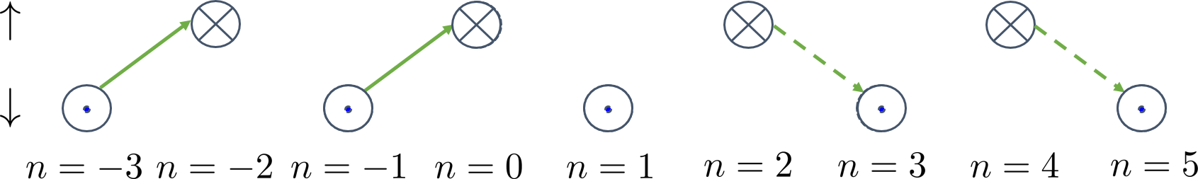
Figure 5: A diagrammatic representation, in terms of the $\tilde{\psi}$ (or $\chi$) modes defined at the beginning of Sec. II.2, of the situation where the coefficient $\tilde{t}^{\prime}$ of the time reversal breaking term changes abruptly from $-\tilde{t}$ to $\tilde{t}$ around $n=1$. A decoupled chiral $\tilde{\psi}$ mode is seen to be localized near the boundary at $n=1$, leading to the conclusion that the gapped surface has a halved fractional quantum Hall effect.

To identify the surface Hall conductance $\sigma_{xy}$ characterizing this gapped state, we change $\tilde{t}^{\prime}$ abruptly from $-\tilde{t}$ to $\tilde{t}$ around the point $n=1$, as demonstrated in Fig. (5). It can be seen that a chiral $\chi$-mode, localized on the boundary, remains decoupled. This mode is identical to the mode residing on the edge of a $\nu=1/m$ Laughlin FQHE state. By invoking the bulk-edge correspondence and noticing that this mode is a result of contributions from the two sides of the boundary, we find that the gapped surface has $\sigma_{xy}=\pm\frac{1}{2m}\frac{e^{2}}{h}.$ We note that since the perturbation defined in Eq. (11) is small compared to the bulk energy gap, the resulting gapless chiral mode and the associated value of $\sigma_{xy}$ must be interpreted as properties of the surface.

Thus, the gapped surface of the fractional strong topological insulator exhibits a halved fractional quantum Hall effect. We emphasize that the above result is not limited to the special choice of parameters, which were tuned to the so called “sweet point” Kitaev (2001); Seroussi et al. (2014), and is in fact true as long as the gap remains open. Physically, deviations from $\tilde{t}^{\prime}=\pm\tilde{t}$ in the two regions introduce a non-zero localization length for the boundary mode.

Alternatively, the fractional Dirac liquid can be gapped out by proximity-coupling to an $s$-wave superconductor, i.e., by breaking charge conservation. A superconducting term which does not violate the modified time-reversal symmetry is given by

$$\tilde{H}_{\varDelta} =\Delta\sum_{n}\int dx\left[\tilde{\psi}_{2n,\uparrow}\tilde{\psi}_{2n+1,\downarrow}\right.$$

$$\left.\phantom{}\phantom{}+\tilde{\psi}_{2n,\uparrow}\tilde{\psi}_{2n-1,\downarrow}+h.c.\right].$$ (13)

Again, the physics becomes simple at a sweet point given by $\Delta=\pm\tilde{t}$. Taking $\Delta=\tilde{t}$, for example, the non-quadratic part of the Hamiltonian can be written as

$$\tilde{H}_{\varDelta}=2i\tilde{t}\sum_{n}\left(-1\right)^{n}\int dx\gamma_{n}^{1}\gamma_{n+1}^{2},$$ (14)

with $\tilde{\psi}_{n,\sigma}=\gamma_{n}^{1}+i\gamma_{n}^{2},$ and $\left(\gamma_{n}^{i}\right)^{\dagger}=\gamma_{n}^{i}$ (notice that we have omitted the spin index, which is fully determined by $n$). The modes $\gamma_{n}^{i}$ are referred to as fractional Majorana modes. Indeed, in the integer case, these become chiral Majorana modes, described by a free Majorana theory. The structure of this Hamiltonian is depicted diagrammatically in Fig. (6b), where the dotted symbols represent the fractional Majorana modes $\gamma_{n}^{1}$ and $\gamma_{n}^{2}$. From the form of Eq. (14), it is clear that the system is gapped. Notice that Eq. (11), describing time-reversal symmetry breaking, can be expressed in terms of the fractional Majorana modes as well. In particular, the non-quadratic part of the Hamiltonian $\tilde{H}_{1}+\tilde{H}_{t}$ with $\tilde{t}^{\prime}=\tilde{t}$ takes the simple form $2i\tilde{t}\sum_{n}\int dx\left(\gamma_{2n+1}^{1}\gamma_{2n}^{2}-\gamma_{2n+1}^{2}\gamma_{2n}^{1}\right)$, which is depicted in Fig. (6a).

Once the surface is gapped by proximity to a superconductor, it forms an exotic time-reversal invariant topological superconductor. We leave the further investigation of such a novel superconducting state to future works.

However, it is illuminating to examine the boundary between a magnetic region with broken time-reversal symmetry, and a superconducting region. The physics is simplest if we gap the region with $n>1$ using a time reversal breaking term of the form (11) with $\tilde{t}^{\prime}=\tilde{t}$, and the region with $n<1$ using a proximity-coupling term of the form (13) with $\Delta=\tilde{t}$. This situation is depicted in Fig. (6c). We see that a decoupled chiral Majorana mode of the form $\gamma_{1}^{1}=\frac{1}{2}\left(e^{im\chi_{1}^{\downarrow}}+e^{-im\chi_{1}^{\downarrow}}\right)$ is localized on the boundary. The propagator describing this fractional Majorana field takes the form $\left\langle\gamma_{1}^{1}(x,t)\gamma_{1}^{1}(0,0)\right\rangle\propto(x+vt)^{-m}$, making it clear that this gapless channel cannot be described by a free Majorana theory. We point out the similarity to the edge mode of the 2D fractional topological superconductor discussed in Ref. Vaezi (2013).

One can generalize the construction to study hierarchical states, with $\nu$ different from $1/m$. Within the simplified model, each layer in Fig. (4a) now contains a FQHE state with a general $K$-matrix of dimension $d$, and therefore $d$ distinct edge modes $\chi_{n}^{j}$ (where $n$ is the layer index and $j=1,\cdots,d$ enumerates the edge modes in a given layer). Switching on terms that preserve the modified time reversal symmetry and couple only modes with the same $j$, we get a generalized fractional Dirac theory associated with any $K$-matrix. It is clear, however, that the generalized fractional Dirac theories are not necessarily protected by symmetries, as some modes can be gapped out by coupling fields with different $j$’s (without breaking time-reversal symmetry).

If we repeat the analysis presented in this section and break the modified time-reversal symmetry (still without coupling modes with different $j$’s), we get a halved fractional Hall conductance of the form $\sigma_{xy}=\frac{\nu e^{2}}{2h}$. Additional coupling between modes with different $j$’s has the potential of changing the Hall conductance. Therefore, if symmetry breaking perturbations are introduced, a number of topologically distinct gapped phases may arise on the surface.

The above analysis relied on a modified time reversal symmetry to directly model the surface using coupled 1D modes. In what follows we treat a 3D model with a local time reversal symmetry. As we will see, the analysis presented in the next sections reproduces the universal results derived here.

IV Fractional Strong topological insulators

IV.1 Construction of 2D fractional topological insulators

In Sec. IV.2-IV.3 we will construct a 3D model for a fractional strong topological insulator. Our starting point will be the 2D construction of a fractional topological insulator which was introduced in Ref. Sagi and Oreg (2014). In this section we review this construction, and introduce the general approach used throughout the rest of this work. Unlike the pervious section (Sec. III), where we used a simplified model with a modified time-reversal symmetry [see Fig. (4a)], here we have a local (unmodified) time reversal symmetry. To avoid confusion, we will use a different set of notations in the analysis that follows.

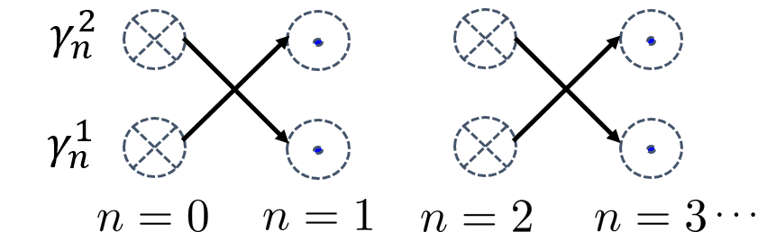
(a)

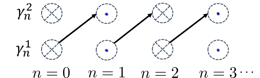
(b)

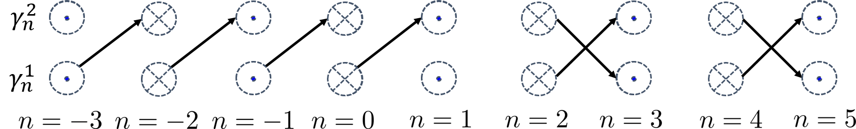
(c)

Figure 6: A diagrammatic representation of the surface model in terms of the fractional Majorana modes $\gamma_{n}^{i}$ (defined after Eq. (14)) in three situations: (a) The modified time reversal symmetry is broken by the perturbation (11) with $\tilde{t}^{\prime}=\tilde{t}$. (b) Charge conservation is broken by a superconducting term of the form (13) with $\Delta=\tilde{t}$. (c) The region with $n<1$ of the surface is gapped by a superconducting term, and the region with $n>1$ is gapped by a modified time-reversal symmetry breaking term. A chiral fractional Majorana mode is attached to the boundary at $n=1$. Here the vertical direction represents the index $i$, and the horizontal direction represents the layer index $n$. Dotted symbols represent the chiral fractional Majorana modes.

IV.1.1 Two-dimensional topological insulator from an array of quantum wires

The 2D model which is the focus of this section is made of $4N$ wires, as depicted in Fig. (7). The $j$’s unit cell is composed of four wires. We note that for convenience the unit cell is shifted by one wire with respect to the unit cell defined in Ref. Sagi and Oreg (2014).

The first and last wires in each unit cell contain electrons, i.e., their highest occupied states are close to the minimum of the conduction band. In a particle-hole symmetric fashion, the two other wires contain holes, i.e., their highest occupied states are close to the maximum of the band.

We describe the system in terms of a tight binding model, where each wire is composed of sites at positions $x=a\cdot i$ (see Fig. (7)). Here $a$ is the distance between adjacent sites, and $i$ is an integer enumerating the sites. Adjacent lattice points are coupled with a hopping amplitude $t_{x}$ ($-t_{x}$) in the electron (hole) wires, as depicted by the arrows in Fig. (7). We define the annihilation operator $\psi_{\alpha,s}^{\left(i,j\right)}$ for an electron with spin $s$ in wire number $\alpha$ ($\alpha=1\ldots 4$) of the unit cell labeled by $\left(i,j\right)$. The Hamiltonian that describes the decoupled wires takes the form $H_{0}=H_{m}+H_{x}$, where

$$H_{m} =m\sum_{i,j}\left(\sum_{\alpha=1,4}\psi_{\alpha,s}^{(i,j)\dagger}\psi_{\alpha,s}^{(i,j)}-\right.$$ (15)

$$\left.-\sum_{\alpha=2,3}\psi_{\alpha,s}^{(i,j)\dagger}\psi_{\alpha,s}^{(i,j)}+h.c.\right),$$

and

$$H_{x} =-t_{x}\sum_{i,j}\left(\sum_{\alpha=1,4}\psi_{\alpha,s}^{(i+1,j)\dagger}\psi_{\alpha,s}^{(i,j)}-\right.$$ (16)

$$\left.-\sum_{\alpha=2,3}\psi_{\alpha,s}^{(i+1,j)\dagger}\psi_{\alpha,s}^{(i,j)}+h.c.\right).$$

The term $H_{x}$ describes intra-wire hopping, and the term $H_{m}$ produces an opposite shift in energy for the electrons and the holes. We note that to have a particle-hole symmetry, the chemical potential is set to be zero. Going to $k$-space, we write $H=\sum_{\mathbf{k}\in BZ1}\vec{\psi}{}^{\dagger}(\mathbf{k})\mathcal{H}(\mathbf{k})\vec{\psi}(\mathbf{k}),$ with $\vec{\psi}=\left(\begin{array}[]{cccccccc}\psi_{1\uparrow}&\psi_{2\uparrow}&\psi_{3\uparrow}&\psi_{4\uparrow}&\psi_{1\downarrow}&\psi_{2\downarrow}&\psi_{3\downarrow}&\psi_{4\downarrow}\end{array}\right)^{T}$. In addition, we define the matrices $\tau_{i}$ ($i=1\ldots 3$) as the Pauli-matrices operating on the wires 1-2 (and 3-4) space. Similarly, the matrices $\sigma_{i}$ operate on the (1,2)-(3,4) blocks, and $s_{i}$ act on the spin degrees of freedom.

In terms of these, the Bloch Hamiltonian corresponding to Eqs. (15)-(16) takes the form

$$\mathcal{H}_{0}=\left[m-2t_{x}\cos\left(k_{x}a\right)\right]\sigma_{z}\tau_{z}.$$ (17)

Furthermore, we introduce Rashba spin-orbit interactions with an alternating coupling $\lambda_{\text{{so}}}\left(-1\right)^{\alpha}$. If the electric field is aligned in the $y$ direction, the resulting term is

$$\mathcal{H}_{\text{so}}=-\lambda_{\text{{so}}}s_{z}\tau_{z}\sin\left(k_{x}a\right).$$ (18)

It proves convenient to define new parameters: $\bar{t}_{x},k_{\text{so}},\text{ and }k_{F}^{0},$ satisfying

$$t_{x} =\bar{t}_{x}\cos\left(k_{\text{so}}a\right),$$ (19)

$$\lambda_{\text{so}} =2\bar{t}_{x}\sin\left(k_{\text{so}}a\right),$$

$$m =2\bar{t}_{x}\cos\left(k_{F}^{0}a\right).$$

In terms of these, it is simple to see that the energy spectra of the four decoupled wires in each unit cell take the form

$$E_{1,s} =2\bar{t}_{x}\left[\cos\left(k_{F}^{0}a\right)-\cos\left(\left(k_{x}-sk_{\text{so}}\right)a\right)\right],$$

$$E_{2,s} =-2\bar{t}_{x}\left[\cos\left(k_{F}^{0}a\right)-\cos\left(\left(k_{x}-sk_{\text{so}}\right)a\right)\right],$$

$$E_{3,s} =-2\bar{t}_{x}\left[\cos\left(k_{F}^{0}a\right)-\cos\left(\left(k_{x}+sk_{\text{so}}\right)a\right)\right],$$

$$E_{4,s} =2\bar{t}_{x}\left[\cos\left(k_{F}^{0}a\right)-\cos\left(\left(k_{x}+sk_{\text{so}}\right)a\right)\right].$$ (20)

If we define the filling factor as

$$\nu=\frac{k_{F}^{0}}{k_{\text{so}}},$$ (21)

the spectra corresponding to the spin-up sector are depicted in Fig. (8a) for the $\nu=1$ case, and in Fig. (8b) for the $\nu=1/3$ case. We now introduce small tunneling operators that couple adjacent wires, and write the inter-wire Hamiltonian in the form $H_{y}+H_{y}^{{}^{\prime}}$, where

$$H_{y} =-t_{y}\sum_{i,j}\left[\psi_{3,s}^{(i,j)\dagger}\psi_{2,s}^{(i,j)}+\psi_{1,s}^{(i,j+1)\dagger}\psi_{4,s}^{(i,j)}+h.c.\right],$$ (22)

$$H_{y}^{{}^{\prime}} =-t_{y}^{\prime}\sum_{i,j}\left[\psi_{2,s}^{(i,j)\dagger}\psi_{1,s}^{(i,j)}+\psi_{4,s}^{(i,j)\dagger}\psi_{3,s}^{(i,j)}+h.c.\right],$$ (23)

with $t_{y},t^{\prime}_{y}\ll\overline{t}_{x}$. The parameter $t_{y}$ describes hopping between two electron-wires or two hole-wires, whereas $t^{\prime}_{y}$ couples the electron and hole wires.

The Bloch Hamiltonian can now be written in the form

$$\mathcal{H} =2\overline{t}_{x}\left[\left(\cos\left(k_{F}^{0}a\right)-\cos\left(k_{x}a\right)\cos\left(k_{so}a\right)\right)\sigma_{z}\tau_{z}-s_{z}\tau_{z}\sin\left(k_{so}a\right)\sin\left(k_{x}a\right)\right]$$

$$\phantom{}\phantom{}-t^{\prime}_{y}\tau_{x}-\frac{t_{y}}{2}\left(\tau_{y}\sigma_{y}+\tau_{x}\sigma_{x}\right)-\frac{t_{y}}{2}\left(\tau_{x}\sigma_{x}-\tau_{y}\sigma_{y}\right)\cos\left(4k_{y}a\right)-\frac{t_{y}}{2}\left(\tau_{x}\sigma_{y}+\tau_{y}\sigma_{x}\right)\sin\left(4k_{y}a\right).$$ (24)

For simplicity, we treat the case where the lattice spacings are identical in the two directions: $a_{x}=a_{y}\equiv a$. This requirement can be lifted without affecting any of the topological properties. Notice that in these conventions, the first Brillouin zone is defined as $k_{y}\in\left(-\frac{\pi}{4a},\frac{\pi}{4a}\right],k_{x}\in\left(-\frac{\pi}{a},\frac{\pi}{a}\right].$

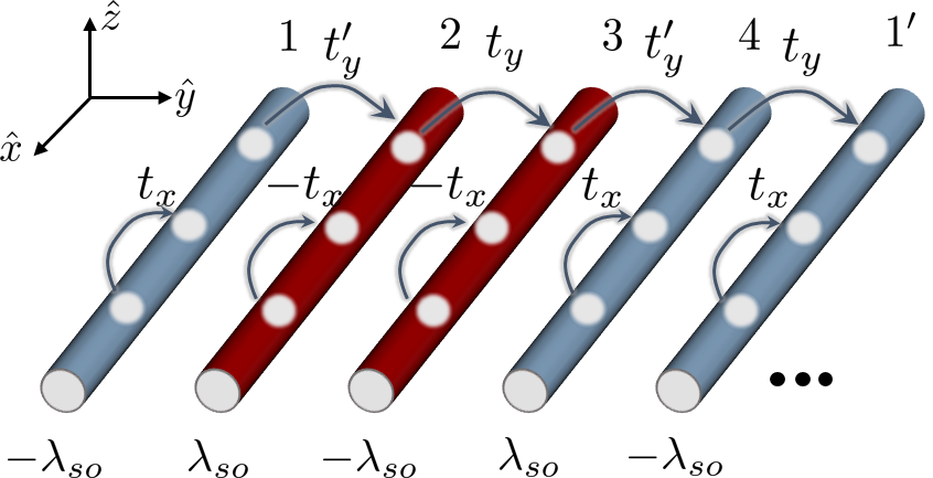
Figure 7: The wire construction we use as a realization of a 2D fractional topological insulator. This model is the starting point in our construction of a 3D fractional strong topological insulator (see Sec. IV.2-IV.3).

We first investigate the integer case, $\nu=1$, where it can be checked from Eq. (24) that as long as $t_{y}\neq t_{y}^{\prime}$ and $t_{y}^{\prime}\neq 0$, the system is completely gapped when periodic boundary conditions are employed. At $t_{y}=t_{y}^{\prime}$ the gap closes, indicating that there might be a phase transition between two topologically distinct phases. To understand the nature of the insulating phases for different values of $t_{y}\text{ and }t^{\prime}_{y}$, it is useful to linearize the spectrum around the Fermi-momenta.

Assuming that $t_{y},t_{y}^{\prime}\ll t_{x}$, the inter-wire terms can be treated as perturbations within the linearized theory. Once the spectrum has been linearized, the only remnants of the original model are the Fermi momenta of the various modes. If momentum conservation is imposed, the values of the Fermi momenta severely restrict the allowed inter-wire coupling terms for a given $\nu$. To keep track of these terms, it is convenient to present the Fermi-momenta as a function of the wire index ($i,\alpha$), as depicted in Fig. (9a) for the spin-up sector.

Again, the symbol $\bigotimes$ ($\bigodot$) represents a right (left) moving mode, and the arrows represent the coupling between different modes, generated by the terms defined in Eqs. (22)-(23).

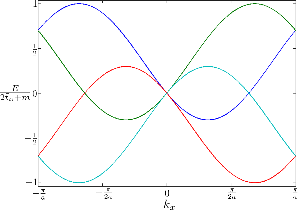
(a)

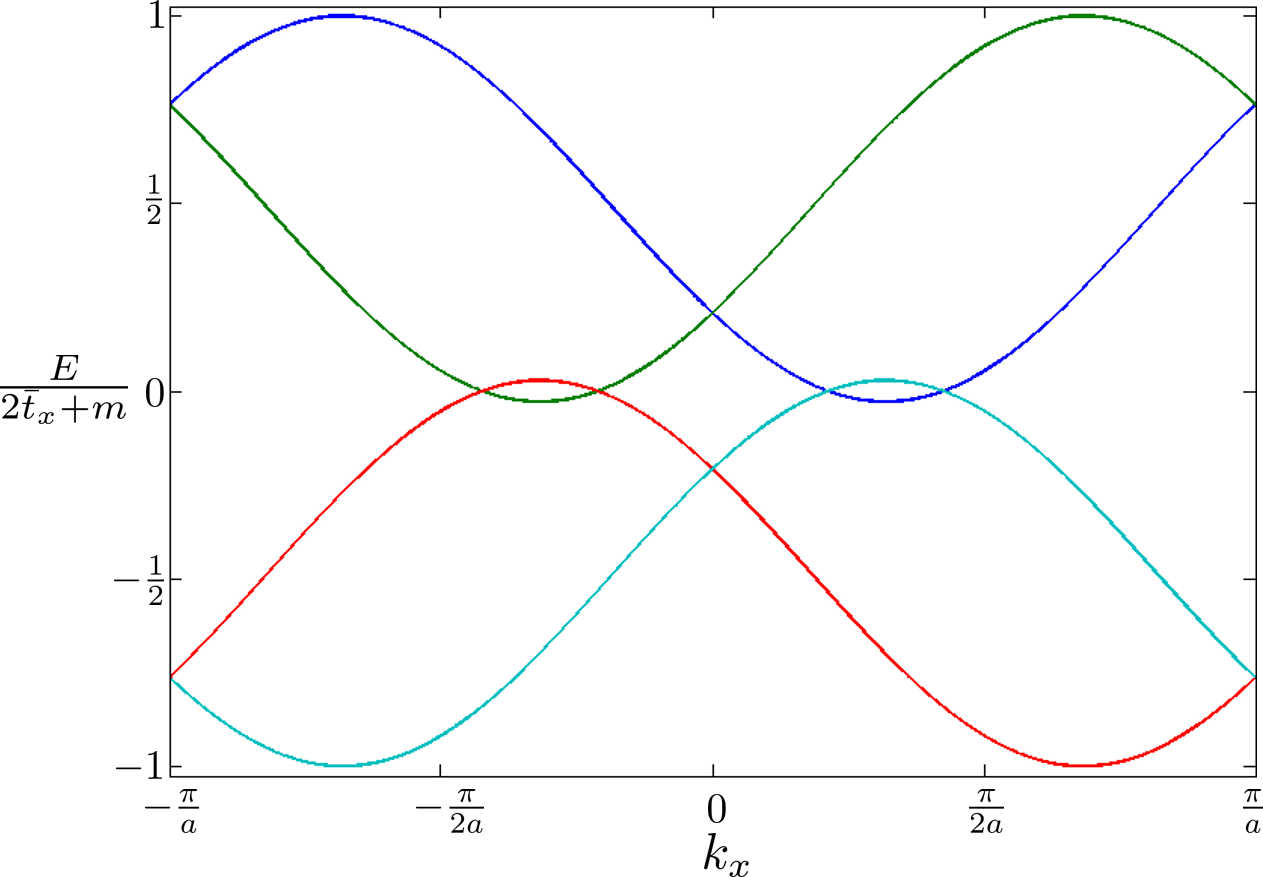
(b)

Figure 8: The spectrum of the system depicted in Fig. (7), when the inter-wire terms are switched off for (a) $\nu=1$, and (b) $\nu=1/3$. We note that only the spin-up sector is presented here. The energies in blue, cyan, red, and green correspond to wires number 1, 2, 3, and 4, respectively.

Since the system is fully gapped for $0<t^{\prime}_{y}<t_{y}$, any such state is adiabatically connected, and therefore topologically equivalent, to the state where $t^{\prime}_{y}$ is negligibly small compared to $t_{y}$. Therefore, it is simple to see that the terms $\psi_{2,\uparrow}^{i,R\dagger}\psi_{3,\uparrow}^{i,L}+h.c.$ and $\psi_{4\uparrow}^{i,R\dagger}\psi_{1,\uparrow}^{i+1,L}+h.c.$ (and in the same way, $\psi_{2,\downarrow}^{i,L\dagger}\psi_{3,\downarrow}^{i,R}+h.c.$ and $\psi_{4\downarrow}^{i,L\dagger}\psi_{1,\downarrow}^{i+1,R}+h.c.$ for the spin-down sector) dominate, and gap the modes near $k_{x}=0$. These terms, however, leave two gapless modes on each edge of the system - one for each spin. For the edge at $i=1$, these edge modes are $\psi_{1,\uparrow}^{1,L},\text{ and }\psi_{1,\downarrow}^{1,R}$. The terms $\psi_{1\uparrow}^{i,R\dagger}\psi_{2,\uparrow}^{i,L}+h.c.$ and $\psi_{3\uparrow}^{i,R\dagger}\psi_{4,\uparrow}^{i,L}+h.c.$ (and in the same way $\psi_{1\downarrow}^{i,L\dagger}\psi_{2,\downarrow}^{i,R}+h.c.$ and $\psi_{3\downarrow}^{i,L\dagger}\psi_{4,\downarrow}^{iR}+h.c.$) are responsible for gapping the modes with $k_{x}\neq 0$. We therefore have a fully gapped bulk with counter-propagating edge modes, protected by time reversal symmetry. Thus, the phase with $t^{\prime}_{y}<t_{y}$ is a topological insulator.

On the other hand, any state with $t^{\prime}_{y}>t_{y}$ is adiabatically connected to the state with $t_{y}=0$, where now the terms $\psi_{1,\uparrow}^{i,L\dagger}\psi_{2,\uparrow}^{i,R}+h.c.$ and $\psi_{3,\uparrow}^{i,L\dagger}\psi_{4,\uparrow}^{i,R}+h.c$. (and in the same way $\psi_{1,\downarrow}^{i,R\dagger}\psi_{2,\downarrow}^{i,L}+h.c.$ and $\psi_{3,\downarrow}^{i,R\dagger}\psi_{4,\downarrow}^{i,L}+h.c$) gap the modes near $k_{x}=0$. In this case we have a fully gapped bulk with no edge modes, indicating that the phase we discuss is topologically trivial.

IV.1.2 Two-dimensional fractional topological insulator from an array of quantum wires

Having found that the above model (defined in Eqs. (15)-(16) and (22)-(23)) can be a topological insulator in the $\nu=1$ case, we now turn to study fractional fillings. We restrict ourselves here to fillings of the form $\nu=1/m$, where $m$ is an odd integer. More general situations were discussed in Ref. Sagi and Oreg (2014).

The diagram that corresponds to the $\nu=1/3$ case is shown in Fig. (9b). It is evident that simple tunneling processes do not conserve momentum and are therefore incapable of gapping the system in this case. Since we are interested in a gapped phase, we have to introduce interactions and consider multi-electron processes.

Fortunately, interaction terms become manageable if we use the standard Abelian bosonization technique. We define the chiral boson fields $\phi_{\alpha,s}^{i,R/L}$, such that $\psi_{\alpha,s}^{i,R/L}\propto\exp\left[i\left(\phi_{\alpha,s}^{i,R/L}+k_{\alpha,s}^{i,R/L}x\right)\right]$, where $k_{\alpha,s}^{i,R/L}$ is the corresponding Fermi-momentum, and the boson fields satisfy the commutation relations

$$\left[\phi_{\alpha,s}^{n,\rho},\phi_{\alpha^{\prime},s^{\prime}}^{n^{\prime},\rho^{\prime}}\right] =i\rho\pi\delta_{s,s^{\prime}}\delta_{\alpha,\alpha^{\prime}}\delta_{\rho,\rho^{\prime}}\delta_{n,n^{\prime}}\text{sign}(x-x^{\prime})$$ (25)

$$\hphantom{d}+i\pi\left(\text{sign}(n-n^{\prime})+\delta_{n,n^{\prime}}\text{sign}(\alpha-\alpha^{\prime})\right)+\delta_{n,n^{\prime}}\delta_{\alpha,\alpha^{\prime}}\pi\left(\sigma_{y}^{s,s^{\prime}}+\delta_{s,s^{\prime}}\sigma_{y}^{\rho,\rho^{\prime}}\right),$$

define new chiral fermion operators according to

$$\tilde{\psi}_{\alpha,s}^{i,R/L} =\left[\psi_{\alpha,s}^{i,R/L}\right]^{\frac{m+1}{2}}\left[\left(\psi_{\alpha,s}^{i,L/R}\right)^{\dagger}\right]^{\frac{m-1}{2}}$$ (26)

$$\propto e^{i\left(\eta_{\alpha,s}^{i,R/L}+q_{\alpha,s}^{i,R/L}x\right)},$$

with

$$\eta_{\alpha,s}^{i,R/L} =\frac{m+1}{2}\phi_{\alpha,s}^{i,R/L}-\frac{m-1}{2}\phi_{\alpha,s}^{i,L/R},$$ (27)

$$q_{\alpha,s}^{i,R/L} =\frac{m+1}{2}k_{\alpha,s}^{i,R/L}-\frac{m-1}{2}k_{\alpha,s}^{i,L/R}.$$ (28)

We note that Eq. (26) makes sense only when the Fermionic operators of the same type are located at close but separate points in space. The commutation relations of the new bosonic $\eta$-fields are

$$\left[\eta_{\alpha,s}^{n,\rho},\eta_{\alpha^{\prime},s^{\prime}}^{n^{\prime},\rho^{\prime}}\right] =i\rho m\pi\delta_{s,s^{\prime}}\delta_{\alpha,\alpha^{\prime}}\delta_{\rho,\rho^{\prime}}\delta_{n,n^{\prime}}\text{sign}(x-x^{\prime})$$ (29)

$$\hphantom{d}+i\pi\left(\text{sign}(n-n^{\prime})+\delta_{n,n^{\prime}}\text{sign}(\alpha-\alpha^{\prime})\right)+\delta_{n,n^{\prime}}\delta_{\alpha,\alpha^{\prime}}\pi\left(\sigma_{y}^{s,s^{\prime}}+m\delta_{s,s^{\prime}}\sigma_{y}^{\rho,\rho^{\prime}}\right).$$

Plotting the diagrams corresponding to the $q$’s, we find that the picture is identical to the one associated with $\nu=1$ (Fig. (9a)). The transformation from the original Fermionic degrees of freedom to the composite $\tilde{\psi}$-fields, which takes a simple linear form in terms of the boson fields, can therefore be interpreted as a transformation from $\nu=1/m$ to $\nu=1$. Hence, in terms of the $\tilde{\psi}$-fields, we can repeat the analysis of the $\nu=1$ case, and write the terms used to obtain a topological insulator. Writing these terms using the $\eta$ bosonic fields, we have:

$$H_{t} =\sum_{i}\left[\int dx\tilde{t}_{y}\cos\left(\eta_{4,\uparrow}^{i,R}-\eta_{1,\uparrow}^{i+1,L}\right)+R\longleftrightarrow L,\uparrow\longleftrightarrow\downarrow\right.$$

$$+\int dx\tilde{t}_{y}\cos\left(\eta_{2,\uparrow}^{i,R}-\eta_{3,\uparrow}^{i,L}\right)+R\longleftrightarrow L,\uparrow\longleftrightarrow\downarrow$$

$$+\sum_{s}\sum_{\rho=R,L}\int dx\tilde{t^{\prime}}_{y}\cos\left(\eta_{1,s}^{i,\rho}-\eta_{2,s}^{i,\overline{\rho}}\right)$$

$$\left.+\sum_{s}\sum_{\rho=R,L}\int dx\tilde{t}^{\prime}_{y}\cos\left(\eta_{3,s}^{i,\rho}-\eta_{4,s}^{i,\overline{\rho}}\right)\right].$$ (30)

Notice that while these are simple tunneling operators in terms of the $\tilde{\psi}$-fields, they describe multi-electron processes of the type depicted by the arrows in Fig. (9b), in terms of the original $\psi$-fields. It was shown in Refs. Kane et al. (2002); Teo and Kane (2014); Oreg et al. (2014) that there is a large range of strong density-density interactions for which such terms flow to the strong coupling limit. Furthermore, for all density-density interactions, the terms $\tilde{t^{\prime}}_{y}$ and $\tilde{t}_{y}$ flow to the strong coupling limit if their bare values are large enough, as their flow diagram coincides with that of the Sine-Gordon model.

Similar to the integer case, if $\tilde{t}^{\prime}_{y}<\tilde{t}_{y}$ the first two terms in Eq. (30) dominate. Assuming they are made relevant, it is evident that the bulk becomes gapped and that the two modes $\eta_{1,\uparrow}^{i,L}\text{ and }\eta_{1,\downarrow}^{i,R}$ remain decoupled. Each of these modes is similar to the edge mode of a $\nu=1/m$ Laughlin QHE state. One can now follow Ref. Teo and Kane (2014) and show that the bulk excitations are fractionally charged and have fractional statistics.

The above analysis suggests that the fractional analog of a given integer topological phase can be realized if we manage to construct the integer phase from an array of coupled wires. Once this is done, we can obtain a fractional phase by considering an analogous system where the $\psi$-fields are replaced by the $\tilde{\psi}$-fields (or equivalently, $\phi$ is replaced by $\eta$), as demonstrated above.

This motivates us to use a similar approach in the construction of fractional phases in 3D. Toward this goal, in the next section we will construct a non-interacting strong topological insulator from an array of wires. Then, in Sec. IV.3 we will study the fractional phase obtained by reducing the filling to $\nu=1/m$, and constructing a strong topological insulator in terms of the composite $\tilde{\psi}$-fields.

IV.2 Strong topological insulators from weakly coupled wires

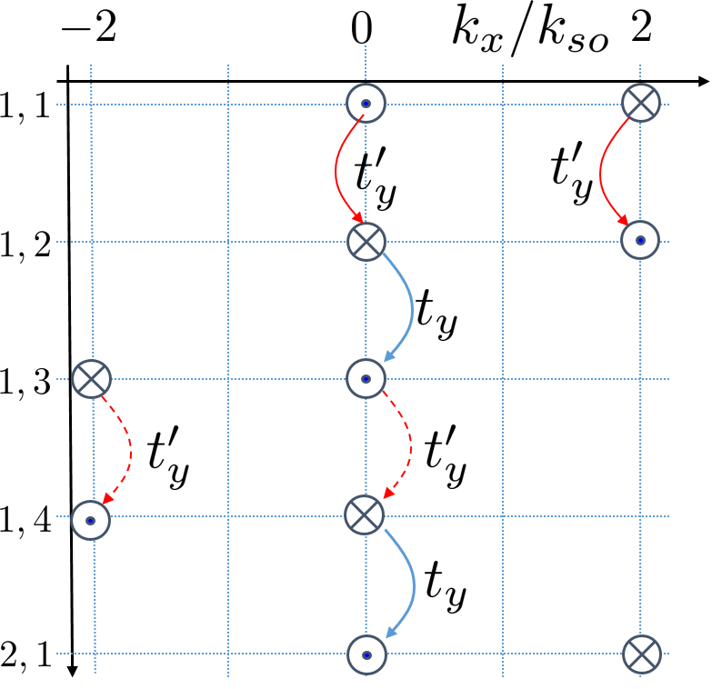
(a)

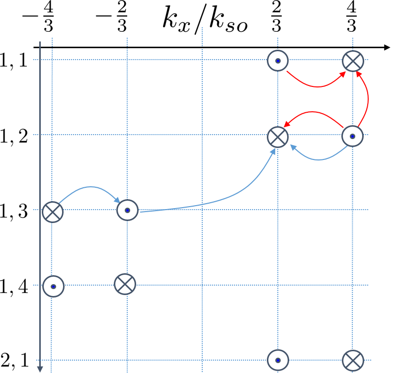
(b)

Figure 9: The diagrams which present the Fermi-momenta of the 2D model as a function of the wire index (labeled by $(i,\alpha)$, where $i$ and $\alpha$ are indices enumerating the unit cells and the position within the unit cell, respectively) for (a) $\nu=1$ , and (b) $\nu=1/3$. Notice that only the modes with spin-up are presented here.

In order to construct a strong topological insulator we stack 2D layers, each made of the wire construction presented in Sec. IV.1, and tune the system such that $\nu=1$. The resulting 3D system is made of an array of wires, as illustrated in Fig. (1). For simplicity, we assume that the distance between adjacent layers is $a$ as well. The goal of this section is to engineer a time-reversal invariant system with a single Dirac cone near the first and last layers.

To do so, we start by tuning each layer to the critical point between the topological and the trivial phase, such that the 2D bulk contains two Dirac modes. This can be achieved by taking $t_{y}=t^{\prime}_{y}$, in which case the Bloch Hamiltonian describing a single layer is given by

$$\mathcal{H} {}_{xy}=2\overline{t}_{x}\left[\left(\cos\left(k_{\text{so}}a\right)-\cos\left(k_{x}a\right)\cos\left(k_{\text{so}}a\right)\right)\sigma_{z}\tau_{z}-s_{z}\tau_{z}\sin\left(k_{\text{so}}a\right)\sin\left(k_{x}a\right)\right]$$

$$\phantom{}\phantom{}\phantom{}\phantom{}-t_{y}\tau_{x}-\frac{t_{y}}{2}\left(\tau_{y}\sigma_{y}+\tau_{x}\sigma_{x}\right)-\frac{t_{y}}{2}\left(\tau_{x}\sigma_{x}-\tau_{y}\sigma_{y}\right)\cos\left(4k_{y}a\right)-\frac{t_{y}}{2}\left(\tau_{x}\sigma_{y}+\tau_{y}\sigma_{x}\right)\sin\left(4k_{y}a\right).$$ (31)

To create a topologically non-trivial gapped 3D phase, we perturb the above gapless Hamiltonian by an inter-layer term of the form

$$\mathcal{H}_{z} =\frac{1}{2}\left[\left(m^{\prime}-2t_{z}\cos\left(k_{z}a\right)\right)\tau_{x}\right.$$ (32)

$$\hphantom{ddddd}\left.+2t^{\prime}_{z}\sin\left(k_{z}a\right)s_{y}\tau_{z}\right]\left(1-\sigma_{x}\right),$$

with $m^{\prime},t_{z},t^{\prime}_{z}\ll t_{y}\ll\bar{t}_{x}$. Unless otherwise noted, we implicitly assume that all the coupling constants are positive.

To see under which circumstances this model forms a strong topological insulator, we now show that if the system is cut at the $z=0$ plane, a single Dirac mode is localized near the resulting surface. It is clear that as long as the inter-layer coupling terms are small, the important degrees of freedom are those close to the Dirac points in each layer. We therefore project the Hamiltonian onto the low-energy subspace of the intra-layer Hamiltonian (Eq. (31)).

The two Dirac cones are located at $k_{x}=k_{y}=0$. Therefore, to identify this low-energy subspace we solve the equation

$$\mathcal{H}_{xy}(k_{x}=k_{y}=0)\psi_{0}=0$$ (33)

for the vectors $\psi_{0}$. The resulting subspace can be spanned by the four vectors $\left|\pm 1,s\right\rangle\equiv\left|\sigma_{x}=-1,\tau_{x}=\pm 1,s\right\rangle$, defined such that $\sigma_{x}\left|\pm 1,s\right\rangle=-\left|\pm 1,s\right\rangle,\tau_{x}\left|\pm 1,s\right\rangle=\pm\left|\pm 1,s\right\rangle,S_{z}\left|\pm 1,s\right\rangle=s\left|\pm 1,s\right\rangle$. In what follows, the basis vectors are ordered as $\{\left|1,\uparrow\right\rangle,\left|-1,\downarrow\right\rangle,\left|1,\downarrow\right\rangle\left|-1,\uparrow\right\rangle\}$. As expected, the $xy$ Hamiltonian, projected onto the low-energy subspace and expanded to first order in momenta, takes the form of two Dirac cones. To be specific, in the above basis the intra-layer Hamiltonian takes the form

$$\mathcal{H}_{xy}=\left(\begin{array}[]{cc}0&h_{\text{Dirac}}\\ h_{\text{Dirac}}^{\dagger}&0\end{array}\right),$$ (34)

where

$$h_{\text{Dirac}}=\left(\begin{array}[]{cc}0&-2\overline{t}_{x}\sin\left(k_{\text{so}}a\right)k_{x}a+2it_{y}k_{y}a\\ 2\overline{t}_{x}\sin\left(k_{\text{so}}a\right)k_{x}a-2it_{y}k_{y}a&0\end{array}\right).$$ (35)

Once the inter-layer part of the Hamiltonian is projected onto the same low energy subspace, it takes the form

$$\mathcal{H}_{z}=\left(\begin{array}[]{cc}h_{\text{1D}}(k_{z})&0\\ 0&h_{\text{1D}}^{*}(k_{z})\end{array}\right),$$ (36)

where $h_{\text{1D}}(k_{z})=\vec{d}\cdot\vec{\sigma}$, with $\vec{d}=\left(0,2t^{\prime}_{z}\sin\left(k_{z}a\right),m^{\prime}-2t_{z}\cos\left(k_{z}a\right)\right)$, can be thought of as the Hamiltonian a 1D model.

If $m^{\prime}<2t_{z}$, the planar vector $\vec{d}$ winds once around the origin as $k_{z}$ winds around the Brillouin zone, indicating that the 1D model is topologically non-trivial. Indeed, in this regime the model can be shown to have zero-energy end modes.

Since the $\hat{z}$ part of our 3D Hamiltonian consists of the two decoupled models $h_{1D}$ and $h_{1D}^{*}$, it produces two zero-energy modes on the $z=0$ surface. It is clear that the full low energy Hamiltonian, projected onto the subspace spanned by these two end modes, must be that of a single Dirac cone.

To see this explicitly, we need an analytic form for the two end modes. This becomes simple if we restrict ourselves to the regime where $2t_{z}$ is close to $m$ and the gap is small. In this limit, focusing again on the low energy properties, we can expand Eq. (36) in small $k_{z}$, and get a continuum model. The model $h_{1D}$ then takes the form

$$h_{1D}\approx\left(\begin{array}[]{cc}m^{\prime}-2t_{z}-t_{z}\partial_{z}^{2}&-2t^{\prime}_{z}a\partial_{z}\\ 2t^{\prime}_{z}a\partial_{z}&-\left(m^{\prime}-2t_{z}-t_{z}\partial_{z}^{2}\right)\end{array}\right)$$ (37)

in the position basis.

Assuming that the system ends at $z=0$, we look for localized zero-energy eigenstates of this Hamiltonian and its complex conjugate, which vanish at $z=0$. Plugging in an exponentially decaying function as an ansatz, we find two such solutions

$$\left|1\right\rangle=\frac{1}{\sqrt{2}}\left(\begin{array}[]{c}1\\ 1\\ 0\\ 0\end{array}\right)f(z),\left|2\right\rangle=\frac{1}{\sqrt{2}}\left(\begin{array}[]{c}0\\ 0\\ 1\\ -1\end{array}\right)f(z),$$ (38)

with $f(z)=\frac{\sqrt{2\lambda_{+}\lambda_{-}\left(\lambda_{+}+\lambda_{-}\right)}}{\lambda_{+}-\lambda_{-}}\left(e^{-\lambda_{+}z}-e^{-\lambda_{-}z}\right)$, and $\lambda_{\pm}=\frac{t^{\prime}_{z}\pm\sqrt{t^{\prime}{}_{z}^{2}+\left(m^{\prime}-2t_{z}\right)t_{z}}}{at_{z}}$.

Projecting the $xy$ part of the Hamiltonian (Eq. (34)), onto the subspace spanned by the two end modes (Eq. (38)), we find a single anisotropic Dirac cone on the surface. The corresponding Hamiltonian takes the form

$$\mathcal{H}_{xy\text{-surface}}=2a\left[k_{y}t_{y}\sigma_{y}+k_{x}t_{x}\sin\left(k_{\text{so}}a\right)\sigma_{x}\right].$$ (39)

Two remarks are in order: first, one can derive the topological nature of the model from the bulk wavefunctions. In fact, recognizing that the system has an inversion symmetry, generated by the operator $\sigma{}_{x}\tau_{x}$, we can implement the procedure introduced in Ref. Fu and Kane (2007) (relating the $\mathbb{Z}_{2}$ invariant to the parity of the occupied states at the time-reversal invariant points) and easily evaluate the $\mathbb{Z}_{2}$ invariant. We have verified that the results of this analysis are consistent with the above derivation, where the surface was studied directly.

Second, we note that since the system is guaranteed to preserve its topological nature as long the gap remains finite, the various parameters are not restricted to the values given above. In particular, the strict requirement $t_{y}=t_{y}^{\prime}$ can be relaxed.

In the next section we study the fractional analog of the model introduced in this section.

IV.3 Fractional strong topological insulators from weakly coupled wires

In Sec. IV.1, when constructing the Laughlin-like $\nu=1/m$ state in 2D, we saw that one can define the $\eta$-fields, in terms of which the problem is mapped to the simple $\nu=1$ case. Reversing the logic, we see that by taking a topological state with $\nu=1$, and replacing the $\phi$ fields by the $\eta$ fields, we expect to get a fractional state.

In this Section, we follow this approach in generalizing our strong topological insulator to its fractional analog. To do so, we start by writing the Hamiltonian of the $\nu=1$ case, discussed in the previous section, in terms of the bosonic $\phi$-fields. Then we write the same Hamiltonian with the $\eta$-fields, and tune the system to filling $\nu=1/m$, where such terms conserve momentum.

We note that all the fields which are not around $k_{x}=0$ are trivially gapped by the intra-layer terms, as seen most clearly in Fig. (9a). Consequently, the topological properties involve only the modes around $k_{x}=0$. In what follows, we therefore write only the operators acting on these fields. In addition, we omit the indices $R/L$, which are fully determined by the spin indices for the $k_{x}=0$ modes.

We define the vector

$$\tilde{\Psi}_{i,n} =\left(\begin{array}[t]{cccc}e{}^{i\eta_{1,\uparrow}^{i,n}}e&{}^{i\eta_{2,\uparrow}^{i,n}}&e^{i\eta_{3,\uparrow}^{i,n}}&e^{i\eta_{4,\uparrow}^{i,n}}\end{array}\right.$$ (41)

$$\hphantom{jijijjjj}\left.\begin{array}[t]{cccc}e^{i\eta_{1,\downarrow}^{i,n}}&e^{i\eta_{2,\downarrow}^{i,n}}&e^{i\eta_{3,\downarrow}^{i,n}}&e^{i\eta_{4,\downarrow}^{i,n}}\end{array}\right)^{T},$$ (43)

where $i$ represents the index enumerating the unit cells in each layer, and $n$ counts the layers. In these notations, the low energy Hamiltonian takes the form

$$H_{x}=\sum_{n,i,\alpha,s}\frac{v}{2\pi m}\int dx\left(\partial_{x}\eta_{\alpha,s}^{i,n}\right)^{2},$$ (44)

$$H_{y}=-t_{y}\sum_{n,i}\int dx\left[\tilde{\Psi}_{i,n}^{\dagger}\left(\tau_{x}+\frac{1}{2}\left(\tau_{y}\sigma_{y}+\tau_{x}\sigma_{x}\right)\right)\tilde{\Psi}_{i,n}+\left(\frac{1}{4}\tilde{\Psi}_{i+1,n}^{\dagger}\left(\tau_{x}+i\tau_{y}\right)\left(\sigma_{x}+i\sigma_{y}\right)\tilde{\Psi}_{i,n}+h.c.\right)\right],$$ (45)

$$H_{z} =\frac{1}{2}\sum_{n,i}\int dx\left[\left(\tilde{\Psi}_{i,n+1}^{\dagger}\left(-t_{z}\tau_{x}+it^{\prime}_{z}s_{y}\tau_{z}\right)\left(1-\sigma_{x}\right)\tilde{\Psi}_{i,n}+h.c\right)+\tilde{\Psi}_{i,n}^{\dagger}m^{\prime}\tau_{x}\left(1-\sigma_{x}\right)\tilde{\Psi}_{i,n}\right].$$ (46)

For simplicity, we do not consider the effects of density-density interactions between the various modes.

We emphasize that analyzing the problem directly in terms of the bosons is essential in the fractional case. Unfortunately, the bosonic form makes it difficult to see that the above set of non-commuting terms results in a gapped system with a gapless surface. In the $\nu=1$ case, we can of course refermionize the above Hamiltonian and repeat the analysis of Sec. IV.2 to show this explicitly. In the fractional case, where refermionization does not result in a solvable model, the situation is more subtle as the various inter-wire terms are irrelevant in the weak coupling limit. To avoid additional complications that arise from that, we work in the regime where the bare amplitudes are large enough such that the inter-wire terms flow to the strong coupling limit and successfully gap out the bulk.

Indeed, if the Hamiltonians $H_{y}$ and $H_{z}$ have very large bare amplitudes, we can neglect the intra-wire terms and the physics becomes practically independent of $m$ because the inter-wire Hamiltonian is quadratic in the fermionic $\tilde{\psi}$-fields. Since we know from the fermionic language that the system is gapped in the $m=1$ case, it is clear that in this limit the same is true for $m>1$. This result is expected to remain true for moderately large bare amplitudes as well.

In what follows, the topological nature of the Hamiltonian is revealed again with the aid of diagrammatic representations. We depict the $\eta$ modes which are not gapped by intra-layer terms (i.e., the modes near $k_{x}=0$) by diagrams of the form shown in Fig. (10).

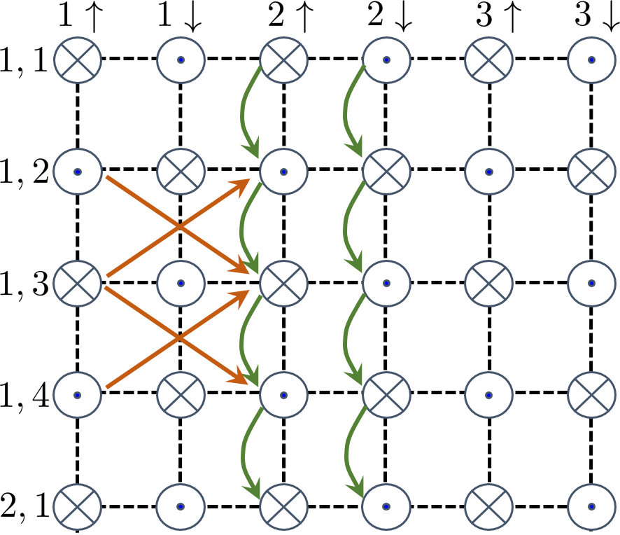
Figure 10: A diagrammatic representation of the reduced 2D tight binding model, describing the inter-wire part of the full 3D model. Here, each “lattice point” corresponds to a linearly dispersing mode in the $x$ direction, with a well defined $y$ and $z$ coordinates. The horizontal axis describes the layer and spin indices ($n,s$), and the vertical axis describes the position within each layer ($i,\alpha$). Again, the symbol $\bigotimes$ ($\bigodot)$ represents a right (left) mover. The green arrows represent the terms in the intra-layer Hamiltonian $H_{y}$, and the brown arrows represent inter-layer terms which couple the spin-up modes, and take the form $-2t_{z}\cos\left(k_{z}a\right)\tau_{x}$ in $k$-space. We emphasize that the reduced model defined in Eq. (45)-(46) contains additional terms which are not depicted here. If all the terms are considered, the full 3D model is topologically non-trivial if the reduced model forms a 2D topological insulator. Thus, the analysis of some aspects of the strongly interacting 3D phase is reduced to the analysis of the 2D non-interacting topological phase.

As before, the symbol $\bigotimes$ ($\bigodot)$ represents a right (left) mover, and colored arrows connecting two modes represent coupling between them. The horizontal axis represents the layer and spin indices ($n,s$), and the vertical axis represents the intra-layer position ($i,\alpha$).

Forgetting for a moment that the symbols represent dispersing 1D modes, if they are treated as states localized on the corresponding lattice points, the diagram presents the 3D problem as a 2D tight-binding model, defined in real space by Eqs. (45)-(46). The 2D lattice model describing the inter-wire coupling terms is referred to as the reduced 2D model. The usefulness of the reduced tight binding model description is revealed by noting that the full 3D model is topologically non-trivial if the reduced model forms a 2D topological insulator.

If the system is infinite (or periodic) in the $\hat{y}$ and $\hat{z}$ directions, the corresponding momenta are good quantum numbers. We therefore write the problem in terms of its Fourier components $k_{y}$ and $k_{z}$. We note that in order to take advantage of the bosonization description, we do not perform a Fourier transform in the $x$ direction. Consequently, the Hamiltonian takes the form

$$H=H_{x}+\sum_{\mathbf{k}}\int dx\tilde{\Psi}_{\mathbf{k}}^{\dagger}(x)\left(h_{y}\left(\mathbf{k}\right)+h_{z}\left(\mathbf{k}\right)\right)\tilde{\Psi}_{\mathbf{k}}(x),$$ (47)

with $\mathbf{k}=\left(k_{y},k_{z}\right)$, and

$$\tilde{\Psi}_{\mathbf{k}}(x)=\frac{1}{\sqrt{N_{y}N_{z}}}\sum_{j,n}e^{-i\left(4jk_{y}a+nk_{z}a\right)}\tilde{\Psi}_{j,n}(x),$$ (48)

$$h_{y}\left(\mathbf{k}\right) =-t_{y}\tau_{x}-\frac{t_{y}}{2}\left(\tau_{y}\sigma_{y}+\tau_{x}\sigma_{x}\right)$$ (49)

$$-\frac{t_{y}}{2}\left(\tau_{x}\sigma_{x}-\tau_{y}\sigma_{y}\right)\cos\left(4k_{y}a\right)$$

$$-\frac{t_{y}}{2}\left(\tau_{x}\sigma_{y}+\tau_{y}\sigma_{x}\right)\sin\left(4k_{y}a\right),$$

$$h_{z}\left(\mathbf{k}\right) =\frac{1}{2}\left[\left(m^{\prime}-2t_{z}\cos\left(k_{z}a\right)\right)\tau_{x}\right.$$ (50)

$$\hphantom{gfgg}+\left.2t^{\prime}_{z}\sin\left(k_{z}a\right)s_{y}\tau_{z}\right]\left(1-\sigma_{x}\right),$$ (51)

where $N_{y}$ is the number of wires in each layer, and $N_{z}$ is the number of layers (cf. Eqs. (31) and (32)).

If the 3D model is finite in the $\hat{y}$ or $\hat{z}$ direction, the reduced 2D model has an edge. For $m^{\prime}<2t_{z}$, it can be checked that the reduced model forms a 2D topological insulator, and has counter propagating edge modes. Recalling that each lattice point in the reduced model represents a linearly dispersing $\eta$-mode, we argue that these edge states correspond to the gapless surface modes of the original 3D model. Therefore, we can get the surface modes by diagonalizing the reduced tight binding model and finding the corresponding edge states.

In order to get an explicit analytic form, we focus again on the regime where $2t_{z}$ is close to $m^{\prime}$, and the gap becomes small. If the system terminates at the $z=0$ plane, the reduced model has two edge modes which take the form

$$\xi_{\beta}(x,k_{y})=\frac{1}{\sqrt{N_{y}}}\sum_{j,n}\sqrt{a}f(a\cdot n)e^{-ijk_{y}a}A_{\beta}\cdot\tilde{\Psi}_{j,n}(x),$$ (52)

where $\beta=1,2$ labels the two counter-propagating edge modes, $f(z)$ is the function defined after Eq. (38), and the vectors $A_{\beta}$ are

$$A_{1} =\frac{1}{4}\left(\begin{array}[t]{cccc}1+i&,1-i&,-i-1&,i-1\end{array}\right.,$$ (54)

$$\left.\begin{array}[t]{cccc}\phantom{,}\phantom{}\hphantom{}\hphantom{}-i+1&,-i-1&,-1+i&,1+i\end{array}\right)$$ (56)

$$A_{2} =A_{1}^{*}.$$ (57)

In the integer case, where $m=1$, Eq. (52) can be thought of as a bosonic description of the Dirac mode localized near the $z=0$ surface (we point out the similarity between the fields defined in Eqs. (52) and (38), up to a different choice of basis). In the fractional case, where $m>1$, the above gapless modes cannot be described by Dirac’s theory of free fermions. As before, we refer to these more general modes as fractional Dirac modes.

The part of the inter-wire Hamiltonian describing the edge modes of the reduced model (which correspond to the surface mode of the original 3D model) takes the form

$$H_{edge} =2t_{y}a\sum_{k_{y}}\int dxk_{y}\vec{\xi}^{\dagger}(x,k_{y})\bar{\tau}_{z}\vec{\xi}(x,k_{y})$$

$$=-2t_{y}i\int dxdy\vec{\xi}^{\dagger}(x,y)\bar{\tau}_{z}\partial_{y}\vec{\xi}(x,y),$$ (58)

where $\vec{\xi}=\left(\begin{array}[t]{cc}\xi_{1}&\xi_{2}\end{array}\right)^{T}$, and $\bar{\tau}_{z}$ is a Pauli matrix acting on this basis. To simplify the analysis presented in the next section, the second line of Eq. (58) was written in the continuum limit.

In the next section we will use the reduced 2D model formalism to study the properties of the surface once it is gapped by breaking its protecting symmetries. We will see that the resulting gapped fractional Dirac modes have unique properties which distinguish them from massive Dirac fermions.

IV.4 Gapping the surface

IV.4.1 Breaking time-reversal symmetry: Halved fractional quantum Hall effect on the surface

Having written a low energy effective surface Hamiltonian using the reduced model, we turn to study what happens when the surface is gapped by breaking time reversal symmetry.

Like in a non-interacting strong topological insulator, we expect the effective action describing the response of our system to the electromagnetic field to contain a $\theta$-term of the form $\frac{\theta}{2\pi}\frac{e^{2}}{2\pi}\int d^{3}xdt\vec{E}\cdot\vec{B}$. In general, time reversal symmetry severely restricts the possible values that the axion angle $\theta$ can take. Naively, one would expect $\theta$ to be either 0, corresponding to a trivial insulator, or $\pi$, corresponding to a topological insulator Qi et al. (2008). However, it was shown in Ref. Maciejko et al. (2010) that fractional axion angles may be consistent with time-reversal symmetry in topologically ordered systems. As we will see, our fractional strong topological insulator provides an example of such a scenario.

In general, the $\theta$-term in the effective action implies that breaking time-reversal symmetry on the surface results in a non-zero surface Hall conductance of the form $\sigma_{xy}=\pm\frac{\theta}{2\pi}\frac{e^{2}}{h}$. In what follows, we calculate $\sigma_{xy}$ directly and then use the above general result to determine the axion angle $\theta$ characterizing our system. To do so, we first break time-reversal symmetry by introducing a Zeeman field $B$ on the surface. We examine a configuration where $B$ changes sign as we cross the line $y=0$. By studying the properties of the gapless mode attached to the boundary, we will be able to deduce the surface Hall conductance.

Within the reduced 2D model formalism, the problem of finding the 1D channel attached to a magnetic domain wall on the surface is converted into that of finding the localized zero-energy mode associated with a similar domain wall on the edge of a 2D topological insulator. To be concrete, we use the continuum model described by Eq. (58) and add a space dependent perturbation of the form $B(y)\vec{\xi}^{\dagger}\bar{\tau}_{x}\vec{\xi}$, where $B(y)=B_{0}\text{sign}\left(y\right)$. This Hamiltonian, and hence the full inter-wire Hamiltonian, has a zero-energy solution of the form

$$\xi_{B}(x)=\sqrt{\lambda_{B}}a\sum_{j,n}f\left(n\cdot a\right)e^{-\lambda_{B}\left|j\right|a}\beta\cdot\tilde{\Psi}_{j,n}(x),$$ (59)

with

$$\beta=\frac{1}{2}\left(\begin{array}[t]{cccccccc}0&1&0&-1&1&0&-1&0\end{array}\right),$$ (60)

and $\lambda_{B}=\frac{B_{0}}{2t_{y}a}$.

Notice that this mode, being a combination of right movers, is a right moving mode. Furthermore, we argue that it is identical to the chiral mode that resides on the edge of a $\nu=1/m$ Laughlin QHE state.

To see this, we calculate the electron propagator characterizing this 1D channel, defined as $G_{B}(x-x^{\prime},t-t^{\prime})=\left\langle\tilde{\xi}_{B}(x^{\prime},t^{\prime})\tilde{\xi}_{B}^{\dagger}(x,t)\right\rangle$. Recall that $\xi_{B}(x)$ is an exact zero-energy solution of the Inter-wire Hamiltonian for any $x$. Therefore, neglecting the coupling to the gapped excitations of the inter-wire Hamiltonian, we can calculate the expectation value with respect to the quadratic intra-wire Hamiltonian shown in Eq. (44) . This results in the propagator

$$G_{B}(x,t)\propto\frac{1}{\left(x-vt\right)^{m}},$$ (61)

which is indeed identical the one characterizing the edge of a $\nu=1/m$ QHE edge state Wen (2007).

Invoking the bulk edge correspondence, we find that $\sigma_{xy}=\pm\frac{1}{2m}\frac{e^{2}}{h}$, in agreement with Sec. III. The halved fractional surface quantum Hall effect indicates that the system is characterized by a fractional axion angle $\theta=\pi/m$. A direct implication of the above is that the system has a fractional magneto-electric response.

We note that to get to Eq. (61) we have used the full intra-wire Hamiltonian, which includes contributions from modes which are already gapped by the inter-wire terms. In doing so, we implicitly assume that the intra-wire Hamiltonian does not couple $\tilde{\xi}_{B}$ to these gapped fields. This can be justified by calculating $\left\langle\left(\tilde{\xi}^{\prime}\right)^{\dagger}H_{x}\tilde{\xi}_{B}\right\rangle,$ where $\tilde{\xi}^{\prime}$ is one of the gapped modes and the average is taken with respect to the intra-wire Hamiltonian. Using the definitions of $\tilde{\xi_{B}}$ and $H_{x}$ [Eqs. (44) and (59)] and the fact that $\tilde{\xi}^{\prime}$ must be orthogonal to $\tilde{\xi_{B}}$, a straightforward calculation shows that this average indeed vanishes, justifying the above calculation.

IV.4.2 Coupling the surface to a superconductor: The emergence of a fractional Majorana mode

Next, we turn to ask what happens when the surface is gapped by breaking charge conservation. This is done by proximity coupling the surface to an $s$-wave superconductor. It was found in Ref. Fu and Kane (2008) that when the surface of a strong topological insulator is gapped in this fashion, the resulting phase resembles a spinless $p_{x}+ip_{y}$ superconductor, but has time-reversal symmetry.

In our model, this problem corresponds to understanding what happens to the edge of the reduced 2D topological insulator when it is coupled to an $s$-wave superconductor. This motivates us to write a proximity term of the form $\Delta\left(\xi_{1}^{\dagger}\xi_{2}^{\dagger}+h.c.\right)$, coupling the two edge modes of the reduced model. Using the enlarged basis, $\vec{\xi}_{N}=\left(\begin{array}[t]{cccc}\xi_{1}(x,y)&\xi_{2}(x,y)&\xi_{2}^{\dagger}(x,y)&\xi_{1}^{\dagger}(x,y)\end{array}\right)^{T}$, we rewrite the edge Hamiltonian in the form

$$\frac{1}{2}\int dxdy\vec{\xi}_{N}^{\dagger}\left(-2it_{y}\tau_{z}\sigma_{z}\partial_{y}+\frac{\Delta}{a}\tau_{z}\sigma_{x}\right)\vec{\xi}_{N}.$$ (62)

In order to reveal the topological nature of the superconducting phase, we consider the boundary between a region with a non-zero $B$ a region with a non-zero $\Delta$. Studying non-interacting strong topological insulators, the authors in Ref. Fu and Kane (2008) have found that such a boundary contains a chiral Majorana mode. We now examine what happens in the fractional case.

In the presence of time-reversal breaking and superconducting terms, the edge part of the reduced Hamiltonian takes the form

$$\frac{1}{2}\int dxdy\vec{\xi}_{N}^{\dagger}\left[-2it_{y}\tau_{z}\sigma_{z}\partial_{y}\right.$$ (63)

$$\left.+\frac{B(y)}{a}\tau_{x}\sigma_{z}+\frac{\Delta(y)}{a}\tau_{z}\sigma_{x}\right]\vec{\xi}_{N}.$$

We consider a simple situation, where $B(y)=B_{0}\Theta(y)$ and $\Delta=\Delta_{0}\Theta(-y)$ (to be concrete, we assume $\Delta_{0}>0,B_{0}>0$).

The Hamiltonian given by Eq. (63) has a zero energy solution of the form

$$\frac{1}{\sqrt{2}}\left(\xi_{B\Delta}+\xi_{B\Delta}^{\dagger}\right),$$ (64)

with

$$\xi_{B\Delta}=\sqrt{\frac{2\lambda_{B}\lambda_{\Delta}}{\lambda_{B}+\lambda_{\Delta}}}a\sum_{j,n}e^{-i\pi/4}f(n\cdot a)\beta\cdot\tilde{\Psi}_{j,n}(x)g(ja),$$ (65)

$$g(y)=\left\{\begin{array}[]{c}e^{-\lambda_{B}y},y>0\\ e^{\lambda_{\Delta}y},y<0\end{array}\right.,$$ (66)

$\lambda_{\Delta}=\frac{\Delta_{0}}{2t_{y}a}$ and $\lambda_{B}=\frac{B_{0}}{2t_{y}a}$. For $m=1$, we find a self-Hermitian combination of right moving fermions, making it a chiral Majorana mode, in agreement with Ref. Fu and Kane (2008). If $m>1$, we find again a self-Hermitian chiral mode. However, in this case it cannot be described by a free Majorana theory. In particular, the tunneling density of states associated with this mode is proportional to $\omega^{m-1}$, as opposed to the free Majorana case, where the density of states is constant. This is in fact similar to the tunneling density of states characterizing the edge of a $\nu=1/m$ Laughlin QHE states. To find this result, one can repeat the process that led to Eq. (61) and write the propagator of the above fractional Majorana mode. The above results are in agreement with Sec. III, where we have used a modified time-reversal symmetry to directly model the surface.

V Discussion

The effects of strong interactions on topological matter is a complex subject, and a very active field of study. The challenge becomes even larger in 3D due to the limited analytical tools, and the technical difficulties in applying the existing numerical methods. The coupled-wires approach has been shown to be useful in the theoretical study of such phases in 2D. Within this approach, the existing machinery for treating 1D interacting systems is used to produce various analytical results, which reflect the topological nature of the phase in question.

In this paper, we have demonstrated that the coupled-wires approach can be used to model and analyze 3D topological systems. We have focused on the fractional counterpart of the well known strong topological insulator, which demonstrates the remarkable physical properties of 3D topologically ordered phases. While it is not trivial to study the bulk excitations and the gapless surface in the current formulation, we were able to analyze the non-trivial characteristics of the surface once it is gapped. In particular, the coupled wires approach has been shown to be very effective in revealing the nature of 1D modes residing in the vicinity of domain walls between distinct gapped regions.

This allowed us to show that if the surface is gapped by breaking time-reversal symmetry, it is characterized by a halved fractional Hall conductivity of the form $\sigma_{xy}=\frac{1}{2m}\frac{e^{2}}{h}$. Furthermore, if the surface is partitioned into a magnetic region and a superconducting region, a novel fractional Majorana mode was shown to emerge on the boundary between them.

It would additionally be interesting to generalize the configuration discussed in Ref. Akhmerov et al. (2009), in which one can study and electrically detect the interferometry of Majorana fermions on the surface of a strong topological insulator, to our fractional case. Such an electronic Mach-Zehnder interferometer is expected to contain signatures that differentiate the fractional Majorana modes from free Majorana modes. This will be elaborated on elsewhere.

The current approach provides a path for constructing the fractional analogues of non-interacting topological phases. It would be interesting to systematically apply this formulation to the different classes found in the periodic table of topological phases Schnyder et al. (2008); Kitaev (2009), as was done for 2D systems in Ref. Neupert et al. (2014a). The current work provides the necessary tools for extensions to 3D phases.

Note added. We point out a recent related work (Ref. Meng (2015)), in which an extension of the coupled-wires approach to 3D was discussed. We note that the phases constructed in the above paper are composed of quantum Hall subsystems, and are therefore fundamentally different from the 3D fractional phases constructed in the current work.