Electronic and Nuclear Quantum Effects on the Ice XI/Ice Ih Phase Transition

Abstract

We study the isotope effect on the temperature of the proton order/disorder phase transition between ice XI and ice Ih, using the quasiharmonic approximation combined with ab initio density functional theory calculations. We show that this method is accurate enough to obtain a phase transition temperature difference between light ice (H₂O) and heavy ice (D₂O) of 6 K as compared to the experimental value of 4 K. More importantly, we are able to explain the origin of the isotope effect on the much debated large temperature difference observed in the phase transition. The source of the difference is directly linked to the physics behind the anomalous isotope effect on the volume of hexagonal ice that was recently explained in [Phys. Rev. Lett. 108, 193003 (2012)]. These results indicate that the same physics might be behind the isotope effects in transition temperatures between other ice phases.

I Introduction

The polymorphism of ice is revealed by its rich phase diagram Bartels-Rausch et al. (2012); Petrenko and Whitworth (2006). The availability of different proton configurations that satisfy Bernal-Fowler “ice-rules” Bernal and Fowler (1933) adds another dimension to this phase diagram, given that the same crystalline structure could exist in proton-ordered and disordered form. This leads to additional phases, separated by their corresponding order/disorder phase transitions, as in the case of ice XI/ice Ih, ice IX/ice III, and ice VIII/ice VII Petrenko and Whitworth (2006).

In this paper we focus on the phase transition between proton-ordered (ice XI) and proton-disordered (ice Ih) hexagonal ice. This phase transition has been subject of a large number of experimentalTajima et al. (1982, 1984); Matsuo et al. (1986); Wooldridge and Devlin (1988); Suga (1997) and theoretical studiesRick (2005); Báez and Clancy (1995); Arbuckle and Clancy (2002); Vlot et al. (1999); Nada and van der Eerden (2003); Sanz et al. (2004); Buch et al. (1998); Kuo et al. (2005); Pan et al. (2008, 2010); Singer et al. (2005); Knight et al. (2006); Schönherr et al. (2014). However, open questions remain about the mechanisms behind the phase transition and the importance of nuclear quantum effects in the temperature of the transition Suga (2005).

Experimentally, it is difficult to observe the phase transition from ice Ih to ice XI. A glass transition occurs at around 100-110 K Wooldridge and Devlin (1988); Suga (1997), diminishing the proton mobility and locking protons in their disordered positions, before they orient to form the proton-ordered ice XI structure. This is overcome by catalyzing ice Ih by KOH Tajima et al. (1982, 1984); Matsuo et al. (1986), which allows the lattice parameters of both proton-ordered ice XI Leadbetter et al. (1985); Howe and Whitworth (1989); Jackson and Whitworth (1995); Line and Whitworth (1996); Jackson et al. (1997); Jackson and Whitworth (1997) and disordered ice Ih Röttger et al. (1994, 2012); Line and Whitworth (1996) to be experimentally measured. The order/disorder phase transition is achieved at 72 K for light Tajima et al. (1982) and 76 K for heavy ice Matsuo et al. (1986). Although the isotope effect on the phase transition temperature is measured to be 4 K, a theoretical explanation for this difference is still missing. Ref. Chan, 1975; Johari and Jones, 1976 associated the origin of the isotope effect on the transition temperature to the difference in vibrational energies between the two phases estimating a $\sim 27$ K isotope effect on the transition temperature, while Ref. Matsuo et al., 1986 sought the explanation in the difference in reorientation of the dipole moments of heavy and light ices and predicted a much smaller $\sim 1$ K isotope effect. However, in both of these studies they assume no isotope effect on the volume of the two ices and they also did not take into account the competing anharmonicities between the intra-molecular covalent bonds and the inter-molecular hydrogen bonds. In this work, we reexamine the issue taking into account these two additional effects, extending a previous work on the anomalies in the isotope effect on the volume of ice Pamuk et al. (2012).

A large literature is devoted to the study of the order/disorder phase transition in hexagonal ice. Two main questions are discussed, (i) the ordering nature in the low temperature phase, and (ii) theory and simulation predictions for the phase transition temperature. Experiments such as neutron diffractionLine and Whitworth (1996); Jackson et al. (1997); Jackson and Whitworth (1997), as well as measurements performed under an electric field Jackson and Whitworth (1995) indicate that the ordered phase has ferroelectric order. However, among theory and simulation works there is a large dispersion of results and lack of agreement Rick (2005); Báez and Clancy (1995); Arbuckle and Clancy (2002); Vlot et al. (1999); Nada and van der Eerden (2003); Sanz et al. (2004); Buch et al. (1998); Kuo et al. (2005); Pan et al. (2008, 2010); Singer et al. (2005); Knight et al. (2006); Schönherr et al. (2014). The predicted low T stable phase depends strongly on the choice of boundary conditions, electrostatic multipoles, and treatment of long range interactions. Rick (2005); Báez and Clancy (1995); Arbuckle and Clancy (2002); Vlot et al. (1999); Nada and van der Eerden (2003); Sanz et al. (2004); Buch et al. (1998). In addition, semi-empirical force field models fitted to reproduce experimental data are not accurate enough to distinguish small energy differences between different proton orderings.

According to Ref. Rick, 2005, the TIP4P-FQ Rick et al. (1994) model predicts the proton-disordered phase to be stable, in agreement with Ref. Buch et al., 1998 where other less known models were studied. On the other hand popular water models like SPC/E Berendsen et al. (1987), TIP4P Jorgensen et al. (1983), TIP5P-E Mahoney and Jorgensen (2000) and NvdE Nada and van der Eerden (2003) models predict the proton ordered phases to be more stable in the low temperature limit. Among these studies, only the NvdE Nada and van der Eerden (2003) model predicts the ferroelectric-ordered phase as the lowest energy phase, in agreement with experiments, while the other three models predict the stable phase to be antiferroelectric-ordered. In this same study, it was also shown that modifying the polarizability of the KW-pol model was enough to favor ferroelectric ordering over disordered configurations at low T Buch et al. (1998). Therefore polarizability is an important factor in obtaining the correct potential energy surface.

The effect of proton disorder on the hexagonal ice structure has also been studied using ab initio density functional theory (DFT). DFT calculations correctly reproduce the lattice structure Kuo et al. (2005), and give the cohesive energy of ferroelectric-ordered ice to be larger than either antiferroelectric-ordered or disordered ices Pan et al. (2008, 2010). That is, ferroelectric-ordered ice is the stable ground state. A recent DFT study of ice slabs shows that contrary to the bulk case, the antiferroelectric-ordered ice is more stable in the case of thin films Parkkinen et al. (2014). DFT-based simulations have also been used to predict the phase transition temperature. A Monte Carlo study, where DFT calculations of hydrogen bond configuration energies are used to parametrize a model to perform Monte Carlo simulations, predicted ice XI as the most stable phase, with a transition temperature of 98 K. Singer et al. (2005); Knight et al. (2006) Another recent DFT-based Monte Carlo study of dielectric properties of ice, predicted the temperature of the order-disorder phase transition to be around 70-80 K Schönherr et al. (2014). The advantage of DFT-based Monte Carlo simulations is that they can explore the configurational entropy of the free energy surface in good detail. However, none of these calculations include zero point nuclear quantum effects, or thereby investigate the transition temperature difference between different isotopes. Our goal is to investigate the order/disorder transition from ferroelectric-ordered ice or antiferroelectric-ordered ice to disordered ice, with different isotopic compositions, from an ab initio perspective, including nuclear quantum effects.

In our study we will also compare a polarizable force field model, TTM3-F Fanourgakis and Xantheas (2008) to DFT calculations for the prediction of the most stable phase at low temperatures including zero point corrections.

II Theory

In a recent study, we explained the anomalous isotope effect on the volume of ice Röttger et al. (1994, 2012); Pamuk et al. (2012), by obtaining the free energy with ab initio DFT within the quasiharmonic approximation. We have shown that the anticorrelation between the intra-molecular OH covalent bonds and the inter-molecular hydrogen bonds makes the volume per molecule of D₂O ice larger than that of H₂O ice Pamuk et al. (2012).

In this work, we extend our study of nuclear quantum effects to analyze the contribution to the order/disorder phase transition using both ab initio DFT functionals and the TTM3-F Fanourgakis and Xantheas (2008) force field model. We investigate both ferroelectric-ordered/disordered and antiferroelectric-ordered/disordered phase transitions. In addition, we analyze the importance of van der Waals forces, by comparing a generalized gradient approximated functional, Perdew-Burke-Ernzerhof (PBE) Perdew et al. (1996), to a van der Waals functionalDion et al. (2004); Román-Pérez and Soler (2009), vdW-DF^PBE . We obtain the temperature dependence of the free energy for both ice phases using the quasiharmonic approximation (QHA), and we compare the phase transition temperature of different isotopes.

II.1 Free Energy within Quasiharmonic Approximation

To account for nuclear quantum effects, quantum harmonic eigenstates are needed as a function of volume $V$, at volumes near $V_{0}$, the “frozen lattice” zero pressure volume that minimizes the Born-Oppenheimer energy, $E_{0}(V)$. To lowest order in a Taylor series around $V_{0}$, we have

$$E_{0}(V)=E_{0}(V_{0})+\frac{B_{0}}{2V_{0}}(V-V_{0})^{2}$$ (1)

and

$$\omega_{k}(V)=\omega(V_{0})\left(1-\gamma_{k}\frac{V-V_{0}}{V_{0}}\right).$$ (2)

$B_{0}$ is the dominant part of the bulk modulus, omitting vibrational corrections which will be discussed in a later paper. The “mode Grüneisen parameters” $\gamma_{k}$ are defined as

$$\gamma_{k}=-\frac{\partial(\ln\omega_{k})}{\partial(\ln V)}=-\frac{V}{\omega_{k}}\frac{\partial\omega_{k}}{\partial V}.$$ (3)

The phonon frequencies, $\omega_{k}$ are calculated at three different volumes. The volume dependence of $\omega_{k}(V)$ is calculated to the linear order. Then the Helmholtz free energy $F(V,T)$  Ziman (1979)of independent harmonic oscillators acquires a volume-dependence through $\omega_{k}(V)$,

$$F(V,T) = E_{0}(V)+$$ (4)

$$\sum_{k}\left[\frac{\hbar\omega_{k}(V)}{2}+k_{B}T\ln\left(1-e^{-\hbar\omega_{k}(V)/k_{B}T}\right)\right]$$

$$-TS_{H}$$

The index $k$ runs over both phonon branches and phonon wave vectors within the Brillouin zone. This “quasiharmonic” approximation is correct to first order for volume derivatives like $P=-(\partial F/\partial V)_{T}$. Higher volume derivatives, such as $B(T)$, in general may require higher volume derivatives of $E_{0}$ and $\omega_{k}$. As shown in our recent contributions Pamuk et al. (2012); Ramírez et al. (2012), the first derivative in eq. 2 is a good approximation for hexagonal ice. The temperature dependence of volume $V_{F_{\rm min}}(T)$ is then found in the usual way by minimizing $F(V,T)$ at fixed $T$, the same as setting $P(T)=0$.

The last part of the free energy, $S_{H}$, is the entropy of the proton disorder. This term is zero for proton-ordered ice phases. For the proton-disordered phase, ice Ih, we use the estimation by Pauling, $S_{H}=Nk_{B}\ln(3/2)$, which was obtained by counting hydrogen orientations that obey the ice rules Pauling (1935), and experimentally confirmed for fully disordered cases Giauque and Stout (1936); Giauque and Ashley (1933). We assume that this term does not change with temperature.

Lastly, the classical limit of the free energy is obtained by taking the high temperature limit of the QHA:

$$F(V,T) = E_{0}(V)+$$ (5)

$$\sum_{k}\left[k_{B}T\ln\left(\frac{\hbar\omega_{k}(V(T))}{k_{B}T}\right)\right]-TS_{H}.$$

II.2 Cohesive Energy

To determine which structure is the most stable one at zero temperature, cohesive energies of ices are calculated without ($E_{c}^{0}$) and with ($E_{c}$) zero point effects. The cohesive energy is defined as the amount the energy of a molecule is lowered in a crystal relative to in vacuum:

$$E_{c}^{0}=\frac{E_{0}^{{\rm ice}}}{N_{{\rm molecules}}}-E_{0}^{{\rm monomer}}$$ (6)

$$E_{c}=\frac{F^{{\rm ice}}(V_{F_{\rm min}},0)}{N_{{\rm molecules}}}-E_{0}^{{\rm monomer}}-E_{vib}^{{\rm monomer}},$$ (7)

where the vibrational energy $\sum_{k}\hbar\omega_{k}/2$ of the three modes of the monomer is $E_{vib}^{\rm{monomer}}$. The classical cohesive energy, $E_{c}^{0}$ is defined in eq. 6 using the Kohn-Sham energies of the ice and monomer; and similarly, the quantum cohesive energy with zero point effects, $E_{c}$ is defined in eq. 7.

III Simulation Details

III.1 System Description

In order to predict the most stable phase of hexagonal ice in the zero temperature limit, we performed total energy calculations of three hexagonal ices with different proton configurations. (i) Ice XI. This is the ferroelectric-proton-ordered ice. Oxygen atoms are constrained to the hexagonal wurtzite lattice and hydrogen atoms are ordered such that ice XI has a net dipole moment along the $\hat{c}$ axis, shown in Fig. 1. Precise measurements of lattice structure of ice XI have shown ferroelectric ordering, with a net dipole moment along the $\hat{c}$-axis. Leadbetter et al. (1985); Howe and Whitworth (1989); Jackson and Whitworth (1995); Line and Whitworth (1996); Jackson et al. (1997); Jackson and Whitworth (1997) There are 4 molecules per formula unit. However, TTM3-F calculations were performed for a $3a\times 2\sqrt{3}a\times 2c$ supercell with 96 molecules, with the same cell size as disordered ice Ih.

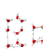
Figure 1: Unit cell of the ferroelectric proton-ordered ice XI structure. The 4 molecules in the unit cell are labeled with a star symbol next to it, and $a$, and $c$ lattice vectors are shown. The image on the left is the side view of the x-z plane; the image on the right is the top view of the x-y plane.

(ii) Ice aXI. We label the antiferroelectric-proton-ordered ice as ice aXI. Ice aXI has 8 molecules in the unit cell. The unit cell is doubled from the ferroelectric proton-ordered ice XI along the x-y plane, with dipole moments of the neighboring molecules pointing in opposite directions such that the system has no net dipole moment, as shown in Fig. 2. Similarly, we have used a unit cell of 8 molecules for the DFT, and 96 molecules for the TTM3-F calculations.

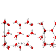
Figure 2: Antiferroelectric proton-ordered ice aXI structure. The 8 molecules in the unit cell are labeled with a star symbol next to it, and $a$, $b$, and $c$ lattice vectors are shown. The image on the left is the side view of the x-z plane; the image on the right is the top view of the x-y plane.

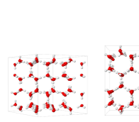
Figure 3: Proton-disordered ice Ih structure. The image on the left is the side view of the x-z plane; the image on the right is the top view of the x-y plane.

(iii) Ice Ih. Experimentally, the lattice structure of light(H₂O) and heavy(D₂O) proton-disordered hexagonal ice Ih have been measured using both syncrotron radiation Röttger et al. (1994, 2012) and neutron diffraction Line and Whitworth (1996), with good agreement. Oxygen atoms still have an underlying hexagonal lattice, while hydrogen atoms are disordered such that it has no net dipole moment. An example of this system is shown in Fig. 3. To accommodate different proton-disordered configurations in ice Ih, we have used a large cell of 96 molecules with dimension $3a\times 2\sqrt{3}a\times 2c$ in our DFT calculations.

We have computed five different 96 molecule configurations of ice Ih using the TTM3-F model. They are generated with an algorithm that goes over all possible allowed proton configurations and produces structures with no net dipole moment Buch et al. (1998).

III.2 Simulation Procedure

We used siesta code Ordejón et al. (1996); Soler et al. (2002) to perform DFT calculations within the generalized gradient approximation (GGA) to the exchange and correlation (XC) functional. The calculations use PBE and vdW-DF^PBE functionals, Perdew et al. (1996); Dion et al. (2004); Román-Pérez and Soler (2009) to compare non-local van der Waals effects with semi-local GGA approximations. These density functionals have previously been shown to give good results for volume calculations of hexagonal ice Ih. Pamuk et al. (2012)

Full structural relaxations for calculating the $E_{0}(V)$ curve are performed with t$\zeta$+p basis. For these relaxations, we have used a real-space mesh cut-off of 500 Ry for the integrals, electronic k-grid cut-off of 10 Å  (corresponding to 38 k-points) for unit cell calculations of ice Ih, force tolerance of 0.001 eV/Å , and a density matrix tolerance of $10^{-5}$ electrons. Instead of doing a variable cell optimization, we calculate the energy of the relaxed structure at a fixed volume for each lattice parameter.

Even though results with the t$\zeta$+p basis are accurate enough to obtain general structural properties Pamuk et al. (2012), for precise order-disorder free energy values, the energy must be very well converged. Recently, a systematic method to obtain the finite-range atomic basis sets for liquid water and ice has been proposed Corsetti et al. (2013). We use the quadruple-$\zeta$ double polarized (q$\zeta$+dp) basis obtained with the new proposed framework. We calculate the energy of the structures again, with the q$\zeta$+dp basis, without relaxation.

For the t$\zeta$+p basis, the error compared to the q$\zeta$+dp basis is $-0.23\%$ in lattice constant $a$, $-0.28\%$ in $c$, and $-0.71\%$ in the total volume. The change in the energy, $E_{0}(V_{0})$ from t$\zeta$+p basis to the q$\zeta$+dp basis without relaxation is 948.6 meV. Further relaxing the structures with the q$\zeta$+dp basis does not change the lattice parameters, and changes the energy only by 1.3 meV. Details of this calculation and the lattice parameters with q$\zeta$+dp basis are given in the Supplemental Material (SM) SM .

For the free energy calculations which include the nuclear quantum effects, the vibrational modes are calculated using the frozen phonon approximation. All the force constant calculations are performed with the t$\zeta$+p basis. There are two reasons for this: the t$\zeta$+p basis gives a good first approximation to the configurational information, and the q$\zeta$+dp basis is costly in computer time. In addition, the largest error in the free energy calculations comes from the initial $E_{0}(V)$ contribution, which we reduce significantly as explained above. The error in the zero point energy contribution is much smaller than the electronic energy error. The force constant calculations of proton-ordered ice XI structure use a finer real-space mesh cut-off of 800 Ry and an atomic displacement of $\Delta x=0.06$ Å. Similarly, the force constant calculations of proton-disordered ice Ih use a real-space mesh cut-off of 500 Ry and an atomic displacement of $\Delta x=0.08$ Å  for the frozen phonon calculations. The acoustic sum rule has been used throughout the study.

The phonon frequencies, $\omega_{k}(V_{0})$ and Grüneisen parameters $\gamma_{k}(V_{0})$ are obtained by diagonalizing the dynamical matrix, computed by finite differences from the atomic forces in a $(3\times 3\times 3)$ supercell, at volumes slightly below and above $V_{0}$. We tested these parameters to obtain force constants in phonon calculations, so that the Grüneisen parameter calculations have minimum noise Pamuk et al. (2012). The Grüneisen parameters are calculated for 3 volumes corresponding to isotropic expansion and compression around the minimum. In order to cover the full Brillouin zone of ice XI and ice aXI, 729 k-points are selected, dividing each reciprocal lattice vector into 9 equal sections.

Table 1: Classical (E${}_{c}^{0}$) and quantum ($E_{c}$ ) cohesive energies, in meV. Quantum values include zero point effects.

FF/XC	Ice	E${}_{c}^{0}$	H2O	D2O	H${}_{2}\text{}^{18}$O
TTM3-F	Ih	601.07$\pm$0.22	521.17$\pm$0.22	536.24$\pm$0.22	522.87$\pm$0.23
TTM3-F	aXI	600.30	520.33	535.41	522.04
TTM3-F	XI	599.71	520.11	535.11	521.81
PBE	Ih	620.44	502.07	526.70	504.15
PBE	aXI	626.21	507.17	531.95	509.25
PBE	XI	629.06	509.02	534.07	511.11
vdW-DFPBE	Ih	723.94	601.64	627.65	603.64
vdW-DFPBE	aXI	725.53	602.58	628.80	604.57
vdW-DFPBE	XI	728.75	605.18	631.52	607.18

IV Results

IV.1 Order-Disorder Phase Transition

To understand the phase transition between proton-disordered and proton-ordered ice, we calculated the cohesive energy from eqs. 6, 7. The cohesive energy including the zero-point nuclear quantum effects are also presented in Table 1. The results from different proton-disordered configurations using the TTM3-F model all lie within $\pm 0.22$ meV of each other, as indicated in the first line of Table 1. The change in the cohesive energy due to the residual entropy of hydrogen disorder is on the order of 0.22 meV, which means that our quantitative prediction of the most stable phase is within this range.

Both DFT functionals predict stability to decrease in the order ice XI $\rightarrow$ ice aXI $\rightarrow$ ice Ih. This agrees with the experiments that the structure of the ordered phase is ferroelectric. On the other hand, TTM3-F predicts the stability order to be the reverse, ice Ih $\rightarrow$ ice aXI $\rightarrow$ ice XI, giving the wrong ground state and no phase transition. Furthermore, considering the error in the cohesive energy, it is impossible to predict the correct stable phase at the zero temperature limit with this model. The phase transition can only be obtained with the DFT calculations.

In order to analyze the proton order-to-disorder phase transition temperature, we study the Helmholtz Free energy at zero pressure. We evaluate the volume dependence of free energy, F(V) at fixed temperature and find the value of free energy minimum, $F(V_{F_{\rm min}}(T))$. Therefore, we obtain a temperature dependence of free energy, by evaluating free energy minimum for each temperature, $F(V_{F_{\rm min}}(T))$, using eq. 5 or 4.

In the classical limit of the free energy, without considering nuclear quantum effects, as given in eq. 5, DFT predicts a phase transition, regardless of the chosen functional. In addition, both semi-local PBE and non-local vdW-DF^PBE functionals overestimate the phase transition temperature, when nuclear quantum effects are not included in the calculations. On the other hand, the TTM3-F force field model does not correctly predict the stable phase in the low temperature limit, and the difference between the free energies of the two phases increases with temperature. Therefore, it does not show a phase transition. We present the full temperature dependence of classical free energy in the SM SM . To understand how each component of eq. 5 contributes to the total free energy, we also present the temperature dependence of $E_{0}(V_{F_{\rm min}}(T))$, and $-TS$ terms separately in the SM SM .

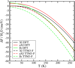
Figure 4: Relative free energy per molecule including the quantum zero point effects as a function of temperature. The lines show DFT results with vdW-DF^PBE functional and the dashed lines are the results with the TTM3-F model. DFT correctly predicts the most stable phase as ice XI for low temperatures, with an energy difference of $\sim$ 4.5 meV. For low temperatures, the TTM3-F model predicts ice Ih as the stable phase with $\sim$ 1 meV energy difference at zero temperature; and a separation of energy at higher temperatures, making the prediction correct for high temperatures only. The results of the TTM3-F model for ice XI and ice aXI represented by black and red dashed lines respectively are almost indistinguishable in this scale.

IV.2 Isotope Effects in the Transition Temperature

Going further, the nuclear zero point effects are calculated to compare the predicted phase transition temperature to the experiments. Fig. 4 shows the temperature dependence of the free energy with zero point effects for H₂O. At all temperatures, TTM3-F model predicts ice Ih to be the stable phase. DFT correctly predicts the most stable phase as the ferroelectric-ordered ice XI for low temperatures, with an energy difference of $\sim$ 4.5 meV. As the temperature increases, there is a crossing at $T=91$ K and the proton-disordered ice Ih becomes the stable phase beyond this temperature for H₂O. DFT predicts antiferroelectric ice aXI to have lower free energy than ice Ih at low T, but at all T, ferroelectric ice XI is preferred to ice aXI. The crossover from the antiferroelectric-ordered ice aXI to proton-disordered ice Ih is at much lower temperatures, because ice aXI is less cohesive than the ferroelectric-ordered ice XI. Therefore, we establish that with DFT, the most stable phase at low temperatures is the ferroelectric-ordered ice XI, in agreement with the experiments. For the rest of the transition temperature discussion, we will focus on the ferroelectric-ordered to disordered transition, ice XI/ice Ih.

Table 2: The classical (T${}_{c}^{0}$) and quantum (T_c) proton order to disorder transition temperature, $T_{c}$ (K) including zero point effects for ice Ih-ice XI and ice Ih-ice aXI. The ratio of the temperature for different isotopes is given as R(D)=D₂O/H₂O and R(¹⁸O)=H${}_{2}\text{}^{18}$O/H₂O, and the isotope effect on the temperature with respect to the H₂O transition temperature is also given as the isotope effect percentage: IS(A-B)=$\frac{T(A)}{T(B)}-1$.

Ice	Method	T${}_{c}^{0}$	H2O	D2O	H${}_{2}\text{}^{18}$O	R(D)	R(18O)	IS(D-H)	IS($\text{}^{18}$O -$\text{}^{16}$O)
aXI	PBE	153	151	156	151	1.03	1.00	$+3.31\%$	$0.00\%$
aXI	vdW-DFPBE	42	30	35	30	1.17	1.00	$+16.67\%$	$0.00\%$
XI	PBE	221	202	215	203	1.06	1.01	$+6.44\%$	$+0.50\%$
XI	vdW-DFPBE	105	91	97	90	1.07	0.99	$+6.59\%$	$-1.10\%$
XI	Expt Tajima et al. (1982); Matsuo et al. (1986)		72	76		1.06		$+5.56\%$

Inclusion of zero point effects also allows us to obtain the isotope effect in the phase transition temperature, since it is experimentally known that the order-disorder transition temperature of heavy ice (D₂O) is higher than light ice (H₂O) by 4 K Tajima et al. (1982); Matsuo et al. (1986). Table 2 shows that we already observe the phase transition with calculations at the classical limit of free energy, for both PBE and vdW-DF^PBE approximations, and that the transition temperature decreases with the inclusion of zero-point effects. The vdW-DF^PBE results are below the glass transition temperature around 100-110 K Wooldridge and Devlin (1988); Suga (1997) where proton mobility diminishes. This is in general agreement with the experimental order-disorder phase transition temperatures. Although PBE gives a correct prediction of the stable phase, and an isotope effect of 6.4$\%$, the value of the phase transition temperature is much larger than the experimental range. In agreement with the experimental 4 K difference in the phase transition temperature of the isotopes, the vdW-DF^PBE functional predicted transition temperature of the heavy ice is larger than the light ice with a 6 K difference. As a result, with this method, the ratio between the phase transition temperatures of heavy and light ice is reproduced within 1% of the experimental value and the isotope effect on the temperature with respect to the H₂O transition temperature is calculated to be 6.6$\%$, as compared to the 5.6$\%$ of the experimental isotope effect. Therefore, it is important to note that inclusion of non-local van der Waals forces is critical for a reasonable prediction of the transition temperature.

Figure 5: Top, free energy difference per molecule between ice Ih and ice XI calculated with vdW-DF^PBE functional in the region of the phase transition. Bottom, contributions to this free energy difference by each term in eq. 4. Left frozen lattice electronic term. Middle zero-point vibrational energy. Right remaining terms. All the energies on the bottom plots have been shifted to allow them to be compared in the same energy scale.

To understand the main reason behind the difference between the transition temperatures of different isotopes, we study the temperature dependence of each component of eq. 4 separately, as presented in Fig. 5. The electronic energy difference between the two ices, $E_{0}({\rm Ih})-E_{0}({\rm XI})$, is larger for H₂O than D₂O. This would result in a larger transition temperature for H₂O than D₂O, contradicting experiments. The last two terms, zero-point-free vibrational entropy and energy $-TS_{v}+E_{v}-E_{ZP}=\sum_{k}k_{B}T\ln\left(1-e^{-\hbar\omega_{k}(V_{F_{\rm min}}(T))/k_{B}T}\right)$, and configurational entropy $-TS_{H}$ also result in larger energy difference for H₂O than D₂O. However, the zero-point vibrational energy $E_{ZP}=\sum_{k}\hbar\omega_{k}(V_{F_{\rm min}}(T))/2$ difference between the two ices, $E_{ZP}({\rm Ih})-E_{ZP}({\rm XI})$, is smaller for H₂O than D₂O. This is the only term that shifts the transition temperature of H₂O below that of D₂O. These results show that the phase transition occurs at a lower $T$ for H₂O than D₂O because of the zero-point energies of the phonon modes.

This can also be seen from a simple model. The transition occurs when the free energies of the two ices are equal. For the sake of simplicity, we can set the zero of energy at the frozen lattice cohesive energy of ice XI and denoting by $E_{d}=E_{0}({\rm Ih})-E_{0}({\rm XI})$ and $S_{H}$ the energy and the residual entropy caused by the disorder of ice Ih. The free energies are $F({\rm XI})=0$ and $F({\rm Ih})=E_{d}-TS_{H}$. Therefore, at the zeroth order, in the classical limit, it follows that $T_{c}(0)=E_{d}/S_{H}$. When the vibrations are included, the free energies from eq. 4 are equal at the transition temperature,

$$T_{c}=\frac{E_{d}}{S_{H}-k_{B}\sum_{k}\ln\left[\frac{\sinh(\hbar\omega_{k}({\rm Ih})/2k_{B}T_{c})}{\sinh(\hbar\omega_{k}({\rm XI})/2k_{B}T_{c})}\right]}.$$ (8)

A more detailed discussion with the high and low $T$ limits of this transition temperature and the latent heat can be found in the SM SM . Assuming the shifts are not large, the isotope shift in the transition temperature can be simplified to

$$\frac{T_{c}^{{\rm D_{2}O}}-T_{c}^{{\rm H_{2}O}}}{T_{c}^{{\rm H_{2}O}}}=\frac{k_{B}T_{c}}{E_{d}}\sum_{k}\ln\left[\frac{R_{k}({\rm Ih})}{R_{k}({\rm XI})}\right]$$ (9)

where

$$R_{k}({\rm Ih})=\frac{\sinh(\hbar\omega_{k}^{{\rm D_{2}O}}({\rm Ih})/2k_{B}T_{c})}{\sinh(\hbar\omega_{k}^{{\rm D_{2}O}}({\rm Ih})/2k_{B}T_{c})},$$ (10)

and similarly for $R_{k}({\rm XI})$. Then the low temperature limit becomes,

$$\frac{\Delta T_{c}({\rm low})}{T_{c}^{{\rm H_{2}O}}}=\frac{\hbar}{2E_{d}}\sum_{k}[ ( \omega_{k}^{{\rm D_{2}O}}({\rm Ih})-\omega_{k}^{{\rm D_{2}O}}({\rm XI}))$$

$$- ( \omega_{k}^{{\rm H_{2}O}}({\rm Ih})-\omega_{k}^{{\rm H_{2}O}}({\rm XI}))]$$ (11)

where the difference in the frequencies exactly corresponds to the energy difference shown in the bottom middle panel of Fig. 5. This model clearly shows that the main source of the isotope effect in the transition temperature is the difference in the zero point energies of the different ices.

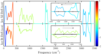
Figure 6: Vibrational density of states for H₂O for proton-ordered ice XI and disordered Ih structures, as obtained with vdW-DF^PBE functional. Average Grüneisen constants of the different modes are given in color code. The inset above zooms into the stretching modes and shows the redshift, while the inset below zooms into the librational modes and shows the blueshift in ice XI with respect to ice Ih.

This is also evident from the phonon density of states of the two ices. Fig. 6 shows phonon density of states for H₂O for both proton-ordered ice XI and proton-disordered ice Ih at zero temperature. The colors represent the average Grüneisen parameter of each band separately. The main effect driving the isotope differences is associated to the blue shift of the librational band in ice XI with respect to ice Ih, and a corresponding redshift of the stretching band. Therefore, with proton ordering, the covalency of the intra-molecular bonds is weakened, while the inter-molecular hydrogen bonding is strengthened. This combined with the weights of the Grüneisen parameters results in an overall slightly larger zero point energy for ice XI than ice Ih.

One of the reasons of the quantitative difference from the experimental results of transition temperature can be due to the error in the estimation of residual entropy from disorder in both systems. Experimentally, it has been shown that at the transition, ice XI loses much but not all of the entropy at $T_{c}$ Line and Whitworth (1996). However, it is not clear whether this arises from equilibrium thermal disorder in ice XI, or from failure to complete the phase transition, leaving some domains of non-equilibrium ice Ih coexisting with ice XI Suga (2005). Another reason for the quantitative difference can be the loss of precision of the QHA at larger temperatures, as the temperature dependence of the phonon vibrations is not taken into account. This is also the case in the calculated $V_{0}$ with isotope effects; the calculated values deviate from the experimental values at larger temperatures Pamuk et al. (2012). However, this deviation is not significant at around 100 K, which is the region of interest of this work.

Finally, the exact values depend on the choice of the DFT functional. While we have shown that the inclusion of vdW interaction in the functional is crucial, it should be noted that the local part of the XC functional also changes the structure significantly. In Ref. Pamuk et al., 2012, it has been shown that vdW-DF functional with the local XC flavor of revPBE softens the structure such that the anomalous isotope effect on the V(T) is not reproduced at low temperatures. In addition, Ref. Murray and Galli, 2012 studied the phonon dispersion of ice XI. While the distribution of the modes are almost identical, the values of the stretching modes are higher and the librational modes are lower by $\sim 50$ cm^-1 than those calculated in this work. Furthermore, Ref. Santra et al., 2013 studied the non-local vdW functionals with different GGA and hybrid functionals for the local XC, and showed that the cohesive energies depend on the choice of these functionals. A hybrid functional with exact exchange for the local XC, with a vdW functional for the non-local correlations could be a good candidate to improve on these results.

All in all, the QHA within DFT with non-local vdW forces, predicts a 6 K temperature difference between the isotopes, as compared to the experimental 4 K difference. This isotope shift is solely due to the nuclear quantum effects from the phonon vibrational energy differences, and it is predicted without invoking any other effects, such as tunneling.

V Conclusion

In this study, we did a detailed analysis of the phase transition between the ferroelectric vs. antiferroelectic-proton-orderered ice XI and disordered ice Ih. Ab initio DFT is necessary to correctly predict the most stable phase of ice as the ferroelectric-ordered ice XI. The TTM3-F force field model needs improvement for the energy predictions, especially at low temperatures.

By including nuclear quantum effects to the free energy, we have predicted the ferroelectric order to disorder phase transition for hexagonal ices. The best accuracy requires using the vdW-DF^PBE functional, with a transition temperature at about 91 K for H₂O and 97 K for D₂O. This 6 K temperature difference is mainly due to the difference in the zero point energy of ice with different isotopes, while entropy related terms contribute in the opposite direction. The method is robust to correctly predict and explain the isotope effect on the order/disorder phase transition of hexagonal ice Ih.

This work is supported by DOE Grants No. DE-FG02-09ER16052 and DE-SC0003871 (MVFS) and DE-FG02-08ER46550 (PBA), and the grant FIS2012-37549-C05 from the Spanish Ministry of Economy and Competitiveness. Research was carried out in part at the Center for Functional Nanomaterials, Brookhaven National Laboratory, which is supported by the U.S. Department of Energy, Office of Basic Energy Sciences, under Contract No. DE-AC02-98CH10886.

References

- Bartels-Rausch et al. (2012) T. Bartels-Rausch, V. Bergeron, J. H. E. Cartwright, R. Escribano, J. L. Finney, H. Grothe, P. J. Gutiérrez, J. Haapala, W. F. Kuhs, J. B. Pettersson, S. D. Price, C. I. Sainz-Díaz, D. J. Stokes, G. Strazzulla, E. S. Thomson, H. Trinks, and N. Uras-Aytemiz, Reviews of Modern Physics 84, 885 (2012).
- Petrenko and Whitworth (2006) V. F. Petrenko and R. W. Whitworth, Physics of Ice (Oxford University Press, 2006).
- Bernal and Fowler (1933) J. D. Bernal and R. H. Fowler, J. Chem. Phys. 1, 515 (1933).
- Tajima et al. (1982) Y. Tajima, T. Matsuo, and H. Suga, Nature 299, 810 (1982).
- Tajima et al. (1984) Y. Tajima, T. Matsuo, and H. Suga, J. Phys. Chem. Solids 45, 1135 (1984).
- Matsuo et al. (1986) T. Matsuo, Y. Tajima, and H. Suga, J. Phys. Chem. Solids 47, 165 (1986).
- Wooldridge and Devlin (1988) P. J. Wooldridge and J. P. Devlin, J. Chem. Phys. 88, 3086 (1988).
- Suga (1997) H. Suga, Thermochimica Acta 300, 117 (1997).
- Rick (2005) S. W. Rick, J. Chem. Phys. 122, 094504 (2005).
- Báez and Clancy (1995) L. A. Báez and P. Clancy, J. Chem. Phys. 103, 9744 (1995).
- Arbuckle and Clancy (2002) B. W. Arbuckle and P. Clancy, J. Chem. Phys. 116, 5090 (2002).
- Vlot et al. (1999) M. J. Vlot, J. Huinink, and J. P. van der Eerden, J. Chem. Phys. 110, 55 (1999).
- Nada and van der Eerden (2003) H. Nada and J. P. J. M. van der Eerden, J. Chem. Phys. 118, 7401 (2003).
- Sanz et al. (2004) E. Sanz, C. Vega, J. L. F. Abascal, and L. G. MacDowell, J. Chem. Phys. 121, 1165 (2004).
- Buch et al. (1998) V. Buch, P. Sandler, and J. Sadlej, J. Phys. Chem. B 102, 8641 (1998).
- Kuo et al. (2005) J.-L. Kuo, M. L. Klein, and W. F. Kuhs, J. Chem. Phys. 123, 134505 (2005).
- Pan et al. (2008) D. Pan, L.-M. Liu, G. A. Tribello, B. Slater, A. Michaelides, and E. Wang, Phys. Rev. Lett. 101, 155703 (2008).
- Pan et al. (2010) D. Pan, L.-M. Liu, G. A. Tribello, B. Slater, A. Michaelides, and E. Wang, J. Phys. Condens. Matter 22, 074209 (2010).
- Singer et al. (2005) S. J. Singer, J.-L. Kuo, T. K. Hirsch, C. Knight, L. Ojamae, and M. L. Klein, Phys. Rev. Lett. 94, 135701 (2005).
- Knight et al. (2006) C. Knight, S. J. Singer, J.-L. Kuo, T. K. Hirsch, L. Ojamae, and M. L. Klein, Phys. Rev. E 73, 056113 (2006).
- Schönherr et al. (2014) M. Schönherr, B. Slater, J. Hutter, and J. VandeVondele, J. Phys. Chem. B 118, 590 (2014).
- Suga (2005) H. Suga, Proc. Japan Acad. Ser. B 81, 349 (2005).
- Leadbetter et al. (1985) A. J. Leadbetter, R. C. Ward, J. W. Clark, P. A. Tucker, T. Matsuo, and H. Suga, J. Chem. Phys. 82, 424 (1985).
- Howe and Whitworth (1989) R. Howe and R. W. Whitworth, J. Chem. Phys. 90, 4450 (1989).
- Jackson and Whitworth (1995) S. M. Jackson and R. W. Whitworth, J. Chem. Phys. 103, 7647 (1995).
- Line and Whitworth (1996) C. M. B. Line and R. W. Whitworth, J. Chem. Phys. 104, 10008 (1996).
- Jackson et al. (1997) S. M. Jackson, V. M. Nield, R. W. Whitworth, M. Oguro, and C. C. Wilson, J. Phys. Chem. B 101, 6142 (1997).
- Jackson and Whitworth (1997) S. M. Jackson and R. W. Whitworth, J. Phys. Chem. B 101, 6177 (1997).
- Röttger et al. (1994) K. Röttger, A. Endriss, J. Ihringer, S. Doyle, and W. F. Kuhs, Acta Cryst. B50, 644 (1994).
- Röttger et al. (2012) K. Röttger, A. Endriss, J. Ihringer, S. Doyle, and W. F. Kuhs, Acta Cryst. B68, 91 (2012).
- Chan (1975) R. K. Chan, Physics and Chemistry of Ice, edited by E. Whalley, S. J. Jones, and L. W. Gold (Roy. Soc. Canada, Ottawa, 1975) p. 306.
- Johari and Jones (1976) G. P. Johari and S. J. Jones, Proc. Roy. Soc. Lond. A 349, 467 (1976).
- Pamuk et al. (2012) B. Pamuk, J. M. Soler, R. Ramirez, C. P. Herrero, P. W. Stephens, P. B. Allen, and M.-V. Fernandez-Serra, Phys. Rev. Lett. 108, 193003 (2012).
- Rick et al. (1994) S. W. Rick, S. J. Stuart, and B. J. Berne, The Journal of Chemical Physics 101, 6141 (1994).
- Berendsen et al. (1987) H. J. C. Berendsen, J. R. Grigera, and T. P. Straatsma, J. Chem. Phys. 91, 6269 (1987).
- Jorgensen et al. (1983) W. L. Jorgensen, J. Chandrasekhar, J. D. M. R. W. Impey, and M. L. Klein, J. Chem. Phys. 79, 926 (1983).
- Mahoney and Jorgensen (2000) M. W. Mahoney and W. L. Jorgensen, J. Chem. Phys. 112, 8910 (2000).
- Parkkinen et al. (2014) P. Parkkinen, S. Riikonen, and L. Halonen, J. Phys. Chem. C 118, 26264 (2014).
- Fanourgakis and Xantheas (2008) G. S. Fanourgakis and S. S. Xantheas, J. Chem. Phys. 128, 074506 (2008).
- Perdew et al. (1996) J. P. Perdew, K. Burke, and M. Ernzerhof, Phys. Rev. Lett. 77, 3865 (1996).
- Dion et al. (2004) M. Dion, H. Rydberg, E. Schröder, D. C. Langreth, and B. I. Lundqvist, Phys. Rev. Lett. 92, 246401 (2004).
- Román-Pérez and Soler (2009) G. Román-Pérez and J. M. Soler, Phys. Rev. Lett. 103, 096102 (2009).
- Ziman (1979) J. M. Ziman, Principles of the Theory of Solids (Cambridge University Press, 1979).
- Ramírez et al. (2012) R. Ramírez, N. Neuerburg, M.-V. Fernández-Serra, and C. P. Herrero, J. Chem. Phys. 137, 044502 (2012).
- Pauling (1935) L. Pauling, J. Am. Chem. Soc. 57, 2680 (1935).
- Giauque and Stout (1936) W. F. Giauque and J. W. Stout, J. Am. Chem. Soc. 58 (7), 1144 (1936).
- Giauque and Ashley (1933) W. F. Giauque and M. F. Ashley, Phys. Rev. 43, 81 (1933).
- Ordejón et al. (1996) P. Ordejón, E. Artacho, and J. M. Soler, Phys. Rev. B 53, 10441 (1996).
- Soler et al. (2002) J. M. Soler, E. Artacho, J. D. Gale, A. García, J. Junquera, P. Ordejón, and D. Sánchez-Portal, J Phys. Condens. Matter 14, 2745 (2002).
- Corsetti et al. (2013) F. Corsetti, M.-V. Fernández-Serra, J. M. Soler, and E. Artacho, J. Phys.: Condens. Matter 25, 435504 (2013).
- (51) See Supplemental Material at http://link.aps.org/supplemental/10.1103/PhysRevB.92.134105 for details of changes in the energy and lattice parameters with different functionals, temperature dependence of the classical limit of the free energy, and the decomposition of different terms of the Helmholtz free energy.
- Murray and Galli (2012) E. D. Murray and G. Galli, Phys. Rev. Lett. 108, 105502 (2012).
- Santra et al. (2013) B. Santra, J. Klimeš, A. Tkatchenko, D. Alfè, B. Slater, A. Michaelides, R. Car, and M. Scheffler, J. Chem. Phys. 139, 154702 (2013).