Submitted to Proceedings of the National Academy of Sciences of the United States of America www.pnas.org/cgi/doi/10.1073/pnas.XXXXXXXXXX Issue Date Issue Number

Submitted to Proceedings of the National Academy of Sciences of the United States of America

Universal Spectrum of Normal Modes in Low-Temperature Glasses: an Exact Solution

Abstract

We report an analytical study of the vibrational spectrum of the simplest model of jamming, the soft perceptron. We identify two distinct classes of soft modes. The first kind of modes are related to isostaticity and appear only in the close vicinity of the jamming transition. The second kind of modes instead are present everywhere in the glass phase and are related to the hierarchical structure of the potential energy landscape. Our results highlight the universality of the spectrum of normal modes in disordered systems, and open the way towards a detailed analytical understanding of the vibrational spectrum of low-temperature glasses.

 
Significance The vibrational spectrum of glasses displays an anomalous excess of soft low-frequency modes with respect to crystals. Such modes are responsible for many anomalies in thermodynamic and transport properties of low-temperature glasses. Many distinct proposals have been formulated to understand their origin but none of them results from the analytic solution of a microscopically grounded model. Here we solve analytically the spectrum of a simple model that belongs to the same universality class of glasses, and identify two distinct mechanisms that are responsible for the soft modes.

 

Introduction –

Low-energy excitations in disordered glassy systems have received a lot of attention because of their multiple interesting features and their importance for thermodynamic and transport properties of low-temperature glasses. Much debate has concentrated around the deviation of the spectrum from the Debye law for solids, due to an excess of low-energy excitations, known as the “boson peak” [1].

The vibrational spectrum of glasses is a natural problem of random matrix theory. In fact, the Hessian of a disordered system is a random matrix due to the random position of particles in the sample. The distribution of the particles induces non trivial correlations between the matrix elements. Many attempted to explain the observed spectrum of eigenvalues by replacing the true statistical ensemble with some simpler ones, in which correlations are neglected or treated in approximate ways [2, 3, 4, 5, 6, 7, 8, 9, 10, 11]. Yet most of these models are not microscopically grounded, thus making it difficult to asses which of the proposed mechanisms are the most relevant and understand their interplay.

In this work we will focus on two ways of inducing a boson peak in random matrix models. First, it has been suggested that the boson peak is due to the vicinity to the jamming transition where glasses are isostatic [12, 13]. Isostaticity means that the number of degrees of freedom is exactly equal to the number of interactions. Isostaticity implies marginal mechanical stability (MMS): cutting one particle contact induces an unstable soft mode, that allows particles to slide without paying any energy cost [14, 15]. From this hypothesis, scaling laws have been derived that characterise the spectrum as a function of the distance from an isostatic point [11, 16, 12]. Secondly, it has been proposed that low-temperature glasses have a complex energy landscape with a hierarchical distribution of energy minima and barriers [17]. Minima are marginally stable [18] and display anomalous soft modes [19, 11] related to the lowest energy barriers [20, 21, 22]. We will denote this second kind of marginality as landscape marginal stability (LMS).

Both mechanisms described above are highly universal. LMS is a generic property of mean field strongly disordered models [18]. MMS holds for a broad class of simple random matrix models [6, 10, 11, 16] and for realistic glass models [12, 23, 24] at the isostatic point. Universality motivates the introduction of a broad class of Continuous Constraint Satisfaction Problems (CCSP) [25], in which a set of constraints is imposed on a set of continuous variables. In the satisfiable (SAT) phase, all the constraints can be satisfied, while this is impossible in the unsatisfiable (UNSAT) phase. A sharp SAT-UNSAT transition separates the two phases: jamming can be seen as a particular instance of this transition. In fact, (i) jamming properties are within numerical precision super-universal, i.e. independent of the spatial dimension $d$ for all $d\geq 2$ [26, 27], (ii) they can be analytically predicted through the exact solution in $d\rightarrow\infty$ [28, 17], and (iii) the perceptron model of neural networks, a prototypical CCSP, displays a jamming transition with the same exponents [25]. Based on universality, both for analytical and numerical computations, the perceptron appears to be the simplest model where low-temperature glassy behaviour can be studied [25].

Here, we exploit this simplicity and characterise analytically the vibrational spectrum of the perceptron at zero temperature in the glass phase. Our main results are: (i) the spectrum is given by a Marchenko-Pastur law with parameters that can be computed analytically; (ii) it closely resembles the one of soft sphere glass models in all $d\geq 2$; (iii) it displays soft modes coming from marginal stabilities of both kinds (LMS and MMS), allowing us to unify both contributions and understand their interplay. Our results are based on the replica method and random matrix theory, and for the first time we are able to derive all the critical properties of jamming within the analytic solution of a well-defined microscopic model.

The model –

We propose to use the perceptron as a minimal model for jamming. In doing that we heavily rely on a universality hypothesis. Rather then looking for physical realism, we posit that we can capture many of the interesting features of low-energy excitations in the glass phase close to jamming making abstraction of the following three basic properties of particle systems: (a) the relevant degrees of freedom, the particle positions, are continuous variables; (b) in hard spheres, impenetrability can be seen as a set of constraints -inequalities- on the distances between spheres; (c) spheres can be made soft by relaxing the impenetrability constraint and imposing a harmonic energy cost to any overlaps [12].

Let us now introduce a general class of CCSP where a set of $N$ continuous variables $x=\{x_{1},...,x_{N}\}$ is subject to a set of $M$ constraints of the form $h_{\mu}(x)>0$ ($\mu=1\cdots M$). The “hard” version of the problem corresponds to allowing only configurations that satisfy the contraints; the “soft” version corresponds to giving an energetic penalty to each violated constraint. This can be encoded in an energy, or Hamiltionian, or “cost” function

$$H[x]=\frac{\varepsilon}{2}\sum_{\mu=1}^{M}h_{\mu}^{2}\theta(-h_{\mu})\ .\hskip 20.0pt$$ (1)

where $\theta(x)$ is the Heaviside function. For all configurations $x$, one obviously has $H[x]\geq 0$. There are thus only two possibilities: either all the constraints can be satisfied and the ground state energy is $H_{GS}=0$ (SAT phase), or $H_{GS}>0$ (UNSAT phase). These two phases are separated, in the thermodynamic limit $N\rightarrow\infty$, by a sharp SAT-UNSAT phase transition [29]. The hard case corresponds to $\varepsilon=\infty$, and the UNSAT phase is then forbidden.

Particle systems correspond to a special choice: the $x_{i}$ are $d$-dimensional vectors confined in a finite fixed volume; each constraint is the “gap” between two given particles, so it has the form $h_{\mu}=|x_{i}-x_{j}|-\sigma$, where $\sigma$ is the particle diameter; the index $\mu=\{i<j\}$ takes $M=N(N-1)/2$ values corresponding to all possible particle pairs. Plugging this in Eq. (1) the reader will immediately recognize the soft sphere Hamiltonian used in most studies on jamming [12, 30]. Because jamming is the point where the energy first becomes non-zero upon increasing $\sigma$, we can identify it with the SAT-UNSAT transition for this special choice of the constraints.

The spherical perceptron is probably the simplest abstract CCSP where, appropriately rephrased, the three ingredients above are combined [25]. The variables $x$ belong to the unitary $N$-dimensional sphere with $\sum_{i}x_{i}^{2}=1$, and one considers $M=\alpha N$ constraints of the form

$$h_{\mu}=\xi^{\mu}\cdot x-\sigma>0\ ,$$ (2)

defined in terms of vectors, $\xi^{\mu}=\{\xi_{1}^{\mu},...,\xi^{\mu}_{N}\}$ composed by quenched i.i.d. random variables with independent $N(0,1)$ components. The control parameters of the system are thus $\alpha$ and $\sigma$, and jamming defines a line in the ($\alpha$, $\sigma$) plane separating the SAT and UNSAT phases. The sign of $\sigma$ is crucial: for $\sigma>0$ the perceptron is a convex CCSP, with a unique energy minimum [31, 32]; for $\sigma<0$ the problem is non-convex and multiple minima are possible [25].

In the following, $\left\langle\bullet\right\rangle$ indicates an average on the minimum energy configurations for a given realisation of quenched disorder (i.e. of the $\xi^{\mu}$) while $\overline{\left\langle\bullet\right\rangle}$ indicates an additional average over the disorder. We will also introduce a special notation for ($\alpha$ times) the average moments of the gap distribution in a given configuration,

$$[h^{n}]=\frac{1}{N}\sum_{\mu=1}^{M}h_{\mu}^{n}\theta(-h_{\mu})\ .$$ (3)

For future reference, it is useful to provide a simple dictionary between physical quantities in particles systems and in the perceptron. The energy is clearly identified with $H\propto[h^{2}]$ in both cases. The pressure is proportional to $\partial H/\partial\sigma\propto[h]$ in particle systems, and the same definition can be used for the perceptron. The gaps between pair of particles correspond to the constraints $h_{\mu}$. The forces, which act from a constraint $\mu$ to a variable $i$, are naturally defined as the $\mu$-contribution to the total force $F_{i}=-\partial H/\partial x_{i}$ acting on $x_{i}$, namely, $f_{i}^{\mu}=-(\partial h_{\mu}/\partial x_{i})h_{\mu}\theta(-h_{\mu})$. The total number of contacts in spheres is the number $N[1]$ of violated constraints with $h_{\mu}\leq 0$; one can keep the same definition for the perceptron. In the following we will approach jamming from the UNSAT phase, where $[h^{n}]\rightarrow 0$ from non-zero values for all $n>0$, while, for continuity, $[1]$ tends to the fraction of binding constraints, i.e. those such that $h_{\mu}=0$. The isostaticity condition is that the number of binding constraints equals the number of degrees of freedom and can be therefore written as $[1]=1$. As already mentioned, $\alpha$ and $\sigma$ play the role of control parameters that are analogue to the packing fraction in the sphere problem. In addition the Debye-Waller factor corresponds to the Edwards-Anderson parameter (see below and [28]). Finally, note that rattlers, i.e. particles that at jamming are involved only in non-binding constraints, cannot exist in the perceptron, because each variable $x_{i}$ is connected to all the constraints.

Vibrational spectrum –

We now present our main technical result which is the exact computation of the eigenvalue spectrum of the Hessian of $H[x]$ in its points of minimum (we now choose $\varepsilon=1$). We enforce the spherical constraint through a Lagrange multiplier $\zeta$ and consider the modified Hamiltonian $H_{\zeta}[x]=H[x]-\frac{N}{2}\zeta(x^{2}-1)$. The first order minimization conditions read

$$\frac{\partial H_{\zeta}}{\partial x_{i}}=\sum_{\mu=1}^{M}\xi_{i}^{\mu}h_{\mu}\theta(-h_{\mu})-N\zeta x_{i}=0\ .$$ (4)

Multiplying by $x_{i}$ and summing over $i$ we can obtain a relation between $\zeta$ and the distribution of the gaps $h_{\mu}$ in the minimum, namely $\zeta=\frac{1}{N}\sum_{\mu}(h_{\mu}^{2}+\sigma h_{\mu})\theta(-h_{\mu})=[h^{2}]+\sigma[h]$. The Hessian matrix, normalized with $N$ reads:

$$M_{ij}=\frac{1}{N}\frac{\partial^{2}H_{\zeta}}{\partial x_{i}\partial x_{j}}=\frac{1}{N}\sum_{\mu=1}^{M}\xi_{i}^{\mu}\xi_{j}^{\mu}\theta(-h_{\mu})-\zeta\delta_{ij}\ .$$ (5)

Notice that in the SAT phase, all the gaps $h_{\mu}$ are positive and both $\zeta$ and the elements of $M$ are trivially equal to zero. We concentrate therefore on the UNSAT phase, where there is a non vanishing fraction $[1]$ of negative gaps $h_{\mu}$.

In principle in the point of minima of $H$, $\xi_{i}^{\mu}\xi_{j}^{\mu}$ and $\theta(-h_{\mu})$ that appear in Eq. (5) could be effectively correlated, however to the leading order in large $N$ these correlations can be neglected, because each $h_{\mu}$ is the sum of a large number of $\xi^{\mu}_{i}$. The matrix $M$ is thus equivalent to a random matrix from a modified Wishart ensemble [33], with an effective number of random contributions equal to $N[1]$ and a constant term $\zeta$ added on the diagonal:

$$M_{ij}\sim\frac{1}{N}\sum_{\mu=1}^{N[1]}\xi_{i}^{\mu}\xi_{j}^{\mu}-\zeta\delta_{ij}=[1]W_{ij}-\zeta\delta_{ij}\ ,$$ (6)

where $W_{ij}=(N[1])^{-1}\sum_{\mu=1}^{N[1]}\xi_{i}^{\mu}\xi_{j}^{\mu}$ is a standard Wishart matrix [34] with “quality factor” $Q=1/[1]$. It follows that for large $N$ the eigenvalue spectrum of $M$ obeys the modified Marchenko-Pastur (MP) law [35]

$$\begin{split}&\rho(\lambda)=\left\{\begin{array}[]{ll}(1-[1])\delta(\lambda+\zeta)+\nu(\lambda)&[1]<1\\ \nu(\lambda)&[1]>1\end{array}\right.\ ,\\ &\nu(\lambda)=\frac{1}{2\pi}\frac{\sqrt{(\lambda-\lambda_{-})(\lambda_{+}-\lambda)}}{\lambda+\zeta}\mathds{1}_{\lambda_{-},\lambda_{+}}(\lambda)\ ,\\ &\lambda_{\pm}=(\sqrt{[1]}\pm 1)^{2}-\zeta\ .\end{split}$$ (7)

This result is very general: for any minimum of $H$, Eq. (LABEL:eq:7) holds for specific values of the parameters $[1]$ and $\zeta$. Also, the eigenvectors of Wishart matrices are delocalized [36] and are asymptotically distributed according to the uniform Haar measure on the sphere. The same properties hold for the eigenvectors of the Hessian of the perceptron. We will see that Eq. (LABEL:eq:7) reproduces all the known features of low-energy excitations close to jamming: its main virtue is to relate these features to a few characteristics of the gap distribution.

The condition of minimum of $H$ requires that all the eigenvalues of the spectrum are positive or zero. For $[1]<1$, this implies $\zeta\leq 0$, which can only happen if $\sigma>0$. Thus for $\sigma<0$, necessarily $[1]\geq 1$. In that case we need $\lambda_{-}\geq 0$, i.e.

$$(\sqrt{[1]}-1)^{2}\geq\zeta=[h^{2}]+\sigma[h]\ .$$ (8)

Equality in Eq. (8) corresponds to a marginally stable minimum whose spectrum touches zero. It also implies that at jamming, where $[h]$ and $[h^{2}]$ vanish and $[1]$ tends to the number of binding constraints, marginally stable minima are necessarily isostatic with $[1]=1$. Note that in the context of sphere packings, Eq. (8) translates into a relation between the excess of contacts $\delta z\sim[1]-1$ and the pressure $p\sim[h]$, which reads $\delta z^{2}\geq Const.\;\times\;p$ and has been derived in [14].

We now need to compute the moments $[h^{n}]$ that enter in Eq. (LABEL:eq:7). Unfortunately, this computation cannot be done analytically for a single minimum or a single sample. Instead, we are able to compute the average $\overline{\left\langle[h^{n}]\right\rangle}$ over all the absolute minima of the Hamiltonian. Because the moments $[h^{n}]$ are self-averaging for large $N$, this provides information over the typical absolute minima of the Hamiltonian as a function of the control parameters $(\alpha,\sigma)$. In the following paragraphs we report the computation of $\overline{\left\langle[h^{n}]\right\rangle}$; for simplicity, unless otherwise specified we drop the averages and replace $\overline{\left\langle[h^{n}]\right\rangle}\rightarrow[h^{n}]$.

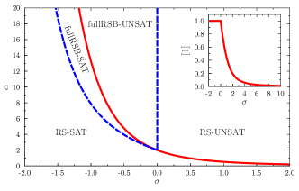
Figure 1: (Main panel) Phase diagram of the model. The RSB region is delimited by the dashed blue line, $\sigma<0$ and $\alpha>\alpha_{c}(\sigma)$. The jamming line $\alpha_{J}(\sigma)$ that separates the SAT from the UNSAT phase, as estimated by the RS solution Eq. (13), is depicted as a full red line. The exact $\alpha_{J}(\sigma)$ should be computed within the fullRSB ansatz for $\sigma<0$, but we expect only a small difference as confirmed in Fig. 3. (Inset) The density of contacts $[1]$ along the jamming line. Jamming is isostatic ($[1]=1$) for $\sigma\leq 0$ and hypostatic ($[1]<1$) for $\sigma>0$.

Thermodynamic analysis: the convex domain –

Thermodynamic and disorder averages can be computed with the aid of the replica method [18]. The partition function is written as an integral over a certain number of copies of the system, the average of the disorder is taken and the resulting integral is evaluated through the saddle-point method for $N\rightarrow\infty$. As a result, one should minimize a free-energy which is a function of the average overlap between replicas, $q_{ab}=\overline{\langle x^{a}\cdot x^{b}\rangle}$ ($q_{aa}=1$ due to the spherical constraint). The minimization is not possible for a generic matrix $q_{ab}$ and one has thus to make an ansatz on the structure of the matrix minimizer, that codes for the organization of the ergodic complonent in the system [18]. If ergodicity holds and there is a single component, the replica symmetric (RS) $q_{ab}=q$ for $a\neq b$ ansatz is appropriate. The RS free energy for the perceptron is [31]

$$F_{RS}=-\frac{T}{2}\left[\log(1-q)+\frac{q}{1-q}\right]-$$ (9)

$$\alpha T\int D_{q}(h+\sigma)\log\left(\int D_{1-q}(y-h)\ e^{-\beta y^{2}\theta(-y)/2}\right)\ ,$$

where $D_{q}(h)=dh\exp[-h^{2}/(2q)]/\sqrt{2\pi q}$ and $D(h)=D_{1}(h)$. This expression must be minimized with respect to $q$.

We have two distinct situations when $T\rightarrow 0$. (i) in the SAT phase, because there are many solutions, different replicas can be in different solutions and $q<1$ at $T=0$ [31]: from Eq. (9) one can show that the ground state energy is $E_{0}=0$. (ii) in the UNSAT phase, the replicas are in the unique absolute energy minimum and $q=1$ at $T=0$. For $T\rightarrow 0$, due to harmonic vibrations, $q=1-\chi T+{\cal O}(T^{2})$. The limit $T\rightarrow 0$ must therefore be taken with $q\rightarrow 1$ and $\chi=\beta(1-q)$ fixed. The parameter $\chi$ diverges approaching the SAT-UNSAT transition from the UNSAT phase, while $q\rightarrow 1$ approaching the transition from the SAT phase.

Let us now focus on the UNSAT phase. Evaluating the most internal integral by saddle point one finds

$$E_{0}=\overline{\left\langle H\right\rangle}=-\frac{1}{2\chi}+\frac{\alpha}{2(1+\chi)}\int_{-\infty}^{0}D(h+\sigma)h^{2}\ ,$$ (10)

and optimizing over $\chi$ gives the equation

$$\left(1+\frac{1}{\chi}\right)^{2}=\alpha\int_{-\infty}^{0}D(h+\sigma)h^{2}\ .$$ (11)

Also, one can show that

$$[h^{n}]=\frac{\alpha}{(1+\chi)^{n}}\int_{-\infty}^{0}D(h+\sigma)h^{n}\ .$$ (12)

Jamming is the point for which $\chi\rightarrow\infty$, or

$$\alpha^{\rm RS}_{J}(\sigma)=\left(\int_{-\infty}^{0}D(h+\sigma)h^{2}\right)^{-1}\ ,$$ (13)

which coincides with the result of [31]. Also, $1/\chi\propto\epsilon$ vanishes linearly in the distance $\epsilon$ from the line $\alpha^{\rm RS}_{J}(\sigma)$, and from Eqs. (11) and (12) we obtain that $E_{0}=[h^{2}]/2=1/(2\chi^{2})\propto\epsilon^{2}$ vanishes quadratically [12, 30]. We can thus identify the line $\alpha^{\rm RS}_{J}(\sigma)$ with the jamming transition, because $E_{0}>0$ for $\alpha>\alpha^{\rm RS}_{J}(\sigma)$ while $E_{0}=0$ for $\alpha\leq\alpha^{\rm RS}_{J}(\sigma)$. From Eqs. (12) and (13) we get $[1]<1$ on the jamming line (Fig. 1), where the system is thus hypostatic and not critical [25].

From Eq. (12) we can compute the moments that enter in Eq. (LABEL:eq:7). Recall that the RS solution implies a unique minimum of the energy, so the average $\overline{\left\langle[h^{n}]\right\rangle}$ coincide with the value of $[h^{n}]$ in the absolute minimum. In the UNSAT phase for $\sigma>0$ we get: (i) for large $\alpha$, $[1]>1$ and $\lambda_{-}>0$: the spectrum is gapped; (ii) for $\alpha\gtrsim\alpha_{J}^{\rm RS}(\sigma)$, $\lambda_{-}>0$ and $[1]<1$ with $\zeta<0$: the spectrum is gapped and it has $1-[1]$ modes with eigenvalue $\lambda=-\zeta>0$; (iii) the same remains true at jamming for $\sigma>0$ and $\alpha=\alpha_{J}^{\rm RS}(\sigma)$, except that the $1-[1]$ modes vanish trivially because $\zeta=0$. When $\sigma\rightarrow 0$, $\lambda_{-}\propto\sigma^{2}$ vanishes so the gap closes on the line $\sigma=0$.

Finally, one can study the stability condition of the RS solution by considering a small perturbation of the matrix $q_{ab}$ and checking if this perturbation lowers the free energy. A standard computation [37, 32] leads to the stability condition. In the SAT phase where $q<1$, the RS stability condition is $\alpha\leq\alpha_{c}(\sigma)$ as computed in [25]; the line $\alpha_{c}(\sigma)$ falls in the SAT region for $\sigma\leq 0$. In the UNSAT phase, we get the condition

$$\left(1+\frac{1}{\chi}\right)^{2}\geq[1]\hskip 10.0pt\Leftrightarrow\hskip 10.0pt\int_{-\infty}^{0}D(h+\sigma)(h^{2}-1)\geq 0\ ,$$ (14)

which is verified for $\sigma\geq 0$ while it is violated for $\sigma<0$.

In summary, for $\sigma<0$ and $\alpha>\alpha_{c}(\sigma)$ the RS solution is unstable (as depicted in Fig. 1) and one must consider a solution for $q_{ab}$ that is not invariant under permutation symmetry, usually denoted a replica symmetry breaking RSB solution [18]. Where the RS solution is correct, the spectrum is gapped.

Thermodynamic analysis: the non-convex domain –

In the region of non convex optimization $\sigma<0$, ergodicity is broken at low temperatures and large $\alpha$. The RS solution is unstable and the structure of the matrix $q_{ab}$ is parametrized by a function $q(x)$ defined in the interval $x\in[0,1]$, which encodes the values of the overlaps of replicas that populate different metastable states of the system. This is called a full replica symmetry breaking (fullRSB) ansatz [18]. In particular this implies that at $T=0$ there are many quasi-degenerate minima of the Hamiltonian. The value of $q(1)=q_{\rm EA}$ is the Edwards-Anderson order parameter that describes the overlap of replicas confined in the same metastable state. The fullRSB equations for the perceptron have been written e.g. in [38]. In general they can only be solved numerically, but the scaling around the jamming transition can be obtained analytically [28, 17, 25]. Here we discuss the main results of this analysis, a detailed derivation will be reported elsewhere.

As in the RS case, $q_{\rm EA}=1-\chi T$ in the UNSAT phase with $\chi\rightarrow\infty$ at the jamming transition. The jamming line falls in the fullRSB region for all $\sigma<0$ (Fig. 1) and can thus be computed numerically solving the fullRSB equations at $T=0$; however, we expect a small difference with the RS computation, and in general the RS result is an upper bound, $\alpha^{\rm fullRSB}_{J}(\sigma)<\alpha^{\rm RS}_{J}(\sigma)$, so we did not perform the fullRSB computation. Let us call once again $\epsilon$ the distance from the jamming line. Combining the results of [28, 17, 25] with original results derived in this work, the following properties can be obtained analytically for $\epsilon\rightarrow 0$:

• the system is isostatic with $[1]=1$ identically for all $\sigma<0$ and $\alpha=\alpha^{\rm fullRSB}_{J}(\sigma)$;

• in the UNSAT phase $\chi\sim\epsilon^{-1/2}$; the average energy vanishes at jamming as $\overline{\left\langle H\right\rangle}\propto[h^{2}]\propto\epsilon^{2}$; the average gap is $[h]\propto\epsilon$; and the excess of contacts above the isostatic value is $[1]-1\sim\epsilon^{1/2}$;

• in the SAT phase, the Edwards-Anderson order parameter behaves as $1-q_{\rm EA}\sim\epsilon^{\kappa}$;

• at jamming ($\epsilon=0$) the probability distribution of the gaps, defined as $g(h)=\text{Prob}(h^{\mu}=h)$ satisfies $g(h)\sim h^{-\gamma}$ for $h\rightarrow 0^{+}$, while the distribution of absolute values of the forces satisfies $P(f)\sim f^{\theta}$ for $f\rightarrow 0^{+}$;

• the values of the critical exponents $\kappa=1.41574\ldots,\ \gamma=0.41269\ldots,\ \theta=0.42311\ldots$ are obtained analytically and coincide with the ones of soft spheres in mean field.

We can next focus on the spectrum and compute $\lambda_{-}$ and $\zeta$ that appear in Eq. (LABEL:eq:7). We obtain that

• $\lambda_{-}$ vanishes identically in the fullRSB phase, because the condition $\lambda_{-}=0$ coincides with the LMS condition. Hence, in the fullRSB UNSAT phase, the spectrum is $\rho(\lambda)\sim\sqrt{\lambda}/(\lambda+\zeta)$ for small $\lambda$ and energy minima are marginally stable.

• $\zeta$ is positive in the UNSAT phase but it goes to zero, as expected, at the jamming transition. Therefore, at jamming $\rho(\lambda)\sim 1/\sqrt{\lambda}$ has a much larger density of soft modes. Slightly away from jamming, $\rho(\lambda)\sim\sqrt{\lambda}$ for $\lambda\ll\zeta$, then reaches a maximum $\rho(\lambda\sim\zeta)\sim 1/\sqrt{\zeta}$, and then decreases as $\rho(\lambda)\sim 1/\sqrt{\lambda}$ for $\lambda\gg\zeta$.

We thus identify two distinct contributions to soft modes: the fullRSB structure (LMS) induces marginality with $\rho(\lambda)\sim\sqrt{\lambda}$ while the proximity to jamming (MMS) induces a much stronger contribution with $\rho(\lambda)\sim 1/\sqrt{\lambda}$.

Note that although each of points (a)-(g) has been derived separately through scaling arguments or numerically [12, 14, 20, 13, 15, 16, 11, 17, 28], here for the first time we derive all of them in a unified way from the analytical solution of a well defined microscopic model.

Comparison with numerical data –

The results of the previous section can be compared with the numerical minimization of the soft perceptron Hamiltonian given in Eq. (1). To obtain numerically the minima of $H$, we use the following procedure. We start from a random assignment $x_{0}$ of the variables and we use the routine gsl_multimin_fdfminimizer_vector_bfgs2 of the GSL library [39], that uses the vector Broyden-Fletcher-Goldfarb-Shanno (BFGS) algorithm to minimize a function. To implement the spherical constraint, we minimize $H_{A}[x]=H[x/|x|]+A(x^{2}-1)^{2}$, where $A$ is an irrelevant number of order 1. Note that this algorithm produces local minima that do not necessarily coincide with the absolute ones in the non-convex domain $\sigma<0$. Therefore, the equilibrium calculation should not necessarily provide exact results for the minima that we produce numerically, however, the differences -if any- between the minima found numerically and the theoretical expectations for the absolute ones are very small. This is probably due to the fact that we work in a regime of fullRSB where relevant metastable states have energy density equal to the one of the ground state [18].

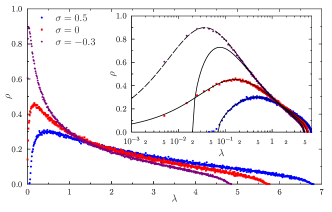
Figure 2: Spectrum of the Hessian for $N=1600$, $\alpha=4$ and $\sigma=0.5,0,-0.3$, averaged over $208$ samples, in linear (main panel) and semilog (inset) scales. The MP law given in Eq. (LABEL:eq:7) with RS parameters (full lines) perfectly reproduces the data for $\sigma\geq 0$, while deviations are observed for $\sigma<0$, where instead a MP law with $\zeta=0.037$ and $[1]=(1+\sqrt{\zeta})^{2}=1.42$ (hence $\lambda_{-}=0$ and $\lambda_{+}=4.76$) perfectly fits the spectrum (dashed line).

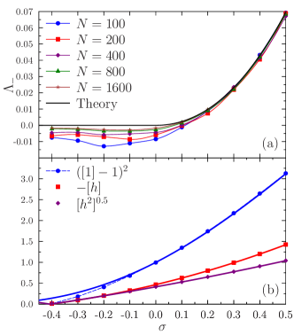
Figure 3: (a) The combination $\Lambda_{-}=(\sqrt{[1]}-1)^{2}-([h^{2}]+\sigma[h])$ as a function of $\sigma$ for $\alpha=4$ and several $N$, averaged over $100$ samples. In the thermodynamic limit this tends to the edge of the spectrum of the Hessian. Stability requires $\Lambda_{-}\geq 0$ for $N\rightarrow\infty$. For $\sigma>0$, $\Lambda_{-}$ tends to values greater than 0 that coincide with the analytical RS result (full line). For $\sigma<0$ the data indicate marginal stability, $\Lambda_{-}\rightarrow 0$ for $N\rightarrow\infty$. (b) The moments $([1]-1)^{2}$, $[h]$ and $\sqrt{[h^{2}]}$ as a function of $\sigma$ for $\alpha=4,N=1600$ (points with dashed lines as guides to the eye). Full lines are the RS predictions. While deviations between theory and simulations are observed in the behaviour of $[1]$, there are no appreciable differences for $[h]$ and $[h^{2}]$. As predicted by the theory these quantities vanish linearly at the jamming point estimated here at $\sigma_{J}\approx-0.409$, which is very well approximated by $\sigma_{J}^{\rm RS}=-0.405234$.

In Fig. 2 we report the spectrum computed numerically and we compare it with the theoretical prediction. As expected, in the RS phase the absolute minimum is unique and can be easily found numerically. Hence, the theoretical prediction perfectly coincides with the analytical result. On the contrary, in the fullRSB phase the numerical algorithm gets stuck into local minima. Yet even in this case the spectrum is described by a Marchenko-Pastur law, which confirms that the result in Eq. (LABEL:eq:7) holds for all minima. Moreover, we find $\lambda_{-}=0$ suggesting that the local minima found by the algorithm are marginally stable.

We checked the expected delocalization properties of the eigenvectors of the Hessian through the statistics of the inverse participation ratio, that for a given normalized eigenvector $v_{i}$ is defined as $y=\sum_{i=1}^{N}v_{i}^{4}$, and is of order $O(1/N)$ for delocalized eigenvectors. We found that the distribution of $y$ is independent of $\alpha$ and $\sigma$. Moreover, the average value of $Ny$ tends to the value $3$ implied by the Haar distribution on the sphere.

In Fig. 3 we report the value of $\Lambda_{-}=(\sqrt{[1]}-1)^{2}-([h^{2}]+\sigma[h])$, where the moments $[h^{n}]$ are evaluated on the numerically obtained minima. According to Eq. (LABEL:eq:7), this quantity should tend to the value of the edge of the spectrum $\lambda_{-}$ in the thermodynamic limit $N\rightarrow\infty$. As expected, we observe that $\Lambda_{-}$ is positive and follows the analytic RS prediction for $\sigma>0$, while for $\sigma<0$ we observe that $\Lambda_{-}\rightarrow 0$ for $N\rightarrow\infty$. Also, in Fig. 3 we report the moments $([1]-1)^{2}$, $[h]$ and $\sqrt{[h^{2}]}$ as a function of $\sigma$ in the UNSAT phase. As predicted by the scaling analysis of the fullRSB solution, these quantities vanish linearly in $\epsilon=\sigma-\sigma_{J}$ where $\sigma_{J}$ is the jamming point. We see therefore that all the regimes predicted by the theory are observed in numerical simulations.

Characteristic frequencies and the boson peak –

We now show that defining the frequency $\omega=\sqrt{\lambda}$ and the density of states $D(\omega)=\rho(\lambda)\frac{d\lambda}{d\omega}$, our spectrum reproduces the salient features of the boson peak phenomenology as described in the introduction. Following [11], we define the characteristic frequencies $\omega_{*}=\sqrt{\zeta}$, $\omega_{0}=\sqrt{\lambda_{-}}$ and $\omega_{\rm max}=\sqrt{\lambda_{+}}$, and from Eq. (LABEL:eq:7) we obtain

$$D(\omega)=\frac{1}{\pi}\frac{\omega\sqrt{(\omega^{2}-\omega_{0}^{2})(\omega_{\rm max}^{2}-\omega^{2})}}{\omega^{2}+\omega_{*}^{2}}\ ,\hskip 10.0pt\omega_{0}\leq\omega\leq\omega_{\rm max}\ .$$ (15)

In the RS phase, we have $\omega_{0}>0$ and the spectrum is gapped, but in a $d$-dimensional, translationally invariant system one should see a Debye spectrum $D(\omega)\sim\omega^{d-1}$ for $\omega<\omega_{0}$. For small $\omega_{0}\ll\omega_{*}$, following [11], one expects in dimension $d$:

$$D(\omega)\sim\begin{cases}\omega^{d-1}&\omega\ll\omega_{0}\ ,\\ \omega^{2}/\omega_{*}^{2}&\omega_{0}\ll\omega\ll\omega_{*}\ ,\\ \text{flat}&\omega_{*}\ll\omega\ll\omega_{\rm max}\ ,\end{cases}$$ (16)

the phononic regime being absent for $d\rightarrow\infty$ and in the perceptron. For $d=3$, $D(\omega)$ displays a crossover between two $\omega^{2}$ regimes at $\omega_{0}$, the second having a larger prefactor because $\omega_{*}$ is small, which results in a boson peak [11].

In the LMS (fullRSB) phase, $\lambda_{-}=0$ and thus $\omega_{0}=0$ identically. We get

$$D(\omega)=\frac{1}{\pi}\frac{\omega^{2}\sqrt{\omega_{\rm max}^{2}-\omega^{2}}}{\omega^{2}+\omega_{*}^{2}}\sim\begin{cases}\omega^{2}&\text{for }\omega\ll\omega_{*}\ ,\\ \text{flat}&\text{for }\omega_{*}\lesssim\omega\leq\omega_{\rm max}\\ \end{cases}$$ (17)

and the phonons should be completely hidden by the soft LMS excitations. Here $\omega_{*}>0$ away from jamming, while $\omega_{*}=\sqrt{\zeta}\sim\sqrt{\sigma[h]}\sim\sqrt{\epsilon}$ when the distance from jamming $\epsilon$ goes to zero.

The result in (17) is fully consistent with the boson peak anomaly in the excitation spectrum of soft sphere packings as known from simulations and scaling arguments [12, 14, 40, 23, 24, 11], confirming the super-universal behavior of glassy systems close to jamming. They are also fully consistent with the results of [11], with the advantage that here we can obtain a fully microscopic expression of the characteristic frequencies $\omega_{0}$ and $\omega_{*}$.

Conclusions –

The soft perceptron is simple enough to allow for a fully analytic characterization of vibrational spectra around UNSAT energy minima. While for any minimum of the Hamiltonian the spectrum has the form of a Marchenko-Pastur law, here we computed the parameters of this distribution only for the absolute minima. Super-universality of the jamming transition allows us to hypothesize that the predicted form and parameter evolution of the spectrum captures many of the low energy features of the spectrum of soft-sphere systems. We find two kinds of soft excitations, as described in [11]. The first ones are related to the existence of a complex energy landscape characterized by a multiplicity of quasi-degenerate marginally stable minima. Due to this landscape marginal stability (LMS), the low-energy spectrum is $D(\omega)\sim\omega^{2}$. The second ones are related to the proximity to an isostatic jamming point, where the spectrum is $D(\omega)\sim\omega^{2}/(\omega^{2}+\epsilon)$. Hence, above a typical frequency $\omega_{*}\sim\epsilon^{1/2}$ the density of states is flat, as found in soft spheres [12, 14]. Note that in particle systems the Debye contribution of phonons to the spectrum scales as $\omega^{d-1}$, hence as soon as $d>3$ the contribution of the LMS soft modes should overcome the one of phonons. In $d=3$ the two contributions are of the same order, and therefore LMS modes might be mixed with phonons. Yet we think that LMS might explain why anomalous soft modes distinct from phonons, that are responsible for the plasticity of the glass, are observed in three dimensional soft sphere packings in the jammed phase for low frequencies $\omega<\omega_{*}$ in the boson peak region [14, 20, 19, 21, 11, 22]. A way to test this idea would be to compute numerically the vibrational spectrum of soft spheres in $d\geq 3$ and investigate the evolution with $d$. Localized soft modes (e.g. the buckling modes discussed in [16, 27]) are also likely to emerge in finite dimensional systems and complicate the analysis.

Let us stress once again that all of our results have been obtained analytically through the exact solution of a well defined model, and there is hope that they will be derived in a mathematically rigorous way in the future. Beyond their direct relevance for the physics of jamming, our results also open a new connection between jamming/packing problems and constraint satisfaction problems with continuous variables, that we conjecture to display a SAT-UNSAT transition in the same (super-)universality class of jamming [25].

The analysis can be extended in several directions. First of all, one can study the spectrum in the SAT (unjammed) phase, corresponding to hard spheres, despite the fact that the energy is zero. In fact, one can study the problem at finite temperature using the Thouless-Anderson-Palmer approach [41, 42] and then take the limit $T\rightarrow 0$ by properly scaling the frequencies [20, 23, 24, 16]. This computation would provide an elegant analytic approach to reproduce the experimental results obtained for colloids in [43, 44]. Other quite straightforward extensions could be the study of the statistics of avalanches [45], and the study of a “quantum perceptron” to investigate how LMS affects the thermodynamic properties in the quantum regime, which could shed light on the mechanisms that induce tunnelling two-level systems in glasses [46].

References

- [1] Malinovsky V, Sokolov A (1986) The nature of boson peak in Raman scattering in glasses. Solid State Communications 57:757–761.
- [2] Schirmacher W, Diezemann G, Ganter C (1998) Harmonic vibrational excitations in disordered solids and the “boson peak”. Physical Review Letters 81:136.
- [3] Grigera T, Martin-Mayor V, Parisi G, Verrocchio P (2003) Phonon interpretation of the ‘boson peak’ in supercooled liquids. Nature 422:289–292.
- [4] Schirmacher W, Ruocco G, Scopigno T (2007) Acoustic attenuation in glasses and its relation with the boson peak. Phys. Rev. Lett. 98:025501.
- [5] Xu N, Wyart M, Liu AJ, Nagel SR (2007) Excess vibrational modes and the boson peak in model glasses. Phys. Rev. Lett. 98:175502.
- [6] Wyart M (2010) Scaling of phononic transport with connectivity in amorphous solids. EPL (Europhysics Letters) 89:64001.
- [7] Zaccone A, Scossa-Romano E (2011) Approximate analytical description of the nonaffine response of amorphous solids. Physical Review B 83:184205.
- [8] Manning ML, Liu AJ (2013) A random matrix definition of the boson peak. arXiv:1307.5904.
- [9] Amir A, Krich JJ, Vitelli V, Oreg Y, Imry Y (2013) Emergent percolation length and localization in random elastic networks. Phys. Rev. X 3:021017.
- [10] Parisi G (2014) Soft modes in jammed hard spheres (i): Mean field theory of the isostatic transition. arXiv:1401.4413.
- [11] DeGiuli E, Laversanne-Finot A, Düring G, Lerner E, Wyart M (2014) Effects of coordination and pressure on sound attenuation, boson peak and elasticity in amorphous solids. Soft Matter 10:5628–5644.
- [12] O’Hern CS, Silbert LE, Liu AJ, Nagel SR (2003) Jamming at zero temperature and zero applied stress: The epitome of disorder. Phys. Rev. E 68:011306.
- [13] Liu A, Nagel S, Van Saarloos W, Wyart M (2011) The jamming scenario – an introduction and outlook eds Berthier L, Biroli G, Bouchaud JP, Cipelletti L, van Saarloos W (Oxford University Press).
- [14] Wyart M, Silbert L, Nagel S, Witten T (2005) Effects of compression on the vibrational modes of marginally jammed solids. Physical Review E 72:051306.
- [15] Wyart M (2012) Marginal stability constrains force and pair distributions at random close packing. Phys. Rev. Lett. 109:125502.
- [16] DeGiuli E, Lerner E, Brito C, Wyart M (2014) Force distribution affects vibrational properties in hard-sphere glasses. Proceedings of the National Academy of Sciences 111:17054–17059.
- [17] Charbonneau P, Kurchan J, Parisi G, Urbani P, Zamponi F (2014) Fractal free energies in structural glasses. Nature Communications 5:3725.
- [18] Mézard M, Parisi G, Virasoro MA (1987) Spin glass theory and beyond (World Scientific, Singapore).
- [19] Xu N, Vitelli V, Liu AJ, Nagel SR (2010) Anharmonic and quasi-localized vibrations in jammed solids‚ modes for mechanical failure. Europhys. Lett. 90:56001.
- [20] Brito C, Wyart M (2009) Geometric interpretation of previtrification in hard sphere liquids. The Journal of Chemical Physics 131:024504.
- [21] Manning ML, Liu AJ (2011) Vibrational modes identify soft spots in a sheared disordered packing. Phys. Rev. Lett. 107:108302.
- [22] Dasgupta R, Karmakar S, Procaccia I (2012) Universality of the plastic instability in strained amorphous solids. Physical review letters 108:075701.
- [23] Mari R, Krzakala F, Kurchan J (2009) Jamming versus glass transitions. Phys. Rev. Lett. 103:025701.
- [24] Ikeda A, Berthier L, Biroli G (2013) Dynamic criticality at the jamming transition. J. Chem. Phys. 138:12A507.
- [25] Franz S, Parisi G (2015) The simplest model of jamming. arXiv:1501.03397.
- [26] Goodrich CP, Liu AJ, Nagel SR (2012) Finite-size scaling at the jamming transition. Physical Review Letters 109:095704.
- [27] Charbonneau P, Corwin EI, Parisi G, Zamponi F (2015) Jamming criticality revealed by removing localized buckling excitations. Phys. Rev. Lett. 114:125504.
- [28] Charbonneau P, Kurchan J, Parisi G, Urbani P, Zamponi F (2014) Exact theory of dense amorphous hard spheres in high dimension. III. the full replica symmetry breaking solution. Journal of Statistical Mechanics: Theory and Experiment 2014:P10009.
- [29] Mézard M, Montanari A (2009) Information, physics, and computation (Oxford University Press).
- [30] Jacquin H, Berthier L, Zamponi F (2011) Microscopic mean-field theory of the jamming transition. Physical review letters 106:135702.
- [31] Gardner E (1988) The space of interactions in neural network models. Journal of physics A: Mathematical and general 21:257.
- [32] Gardner E, Derrida B (1988) Optimal storage properties of neural network models. Journal of Physics A: Mathematical and General 21:271.
- [33] Akemann G, Baik J, Di Francesco P (2011) The Oxford handbook of random matrix theory (Oxford University Press).
- [34] Wishart J (1928) The generalised product moment distribution in samples from a normal multivariate population. Biometrika pp 32–52.
- [35] Marchenko VA, Pastur LA (1967) Distribution of eigenvalues for some sets of random matrices. Matematicheskii Sbornik 114:507–536.
- [36] Bai Z, Miao B, Pan G, et al. (2007) On asymptotics of eigenvectors of large sample covariance matrix. The Annals of Probability 35:1532–1572.
- [37] de Almeida J, Thouless D (1978) Stability of the Sherrington-Kirkpatrick solution of a spin glass model. Journal of Physics A: Mathematical and General 11:983–990.
- [38] Györgyi G, Reimann P (1997) Parisi phase in a neuron. Physical Review Letters 79:2746.
- [39] Galassi M, et al. (2013) GNU Scientific Library Reference Manual, v1.16 (Network Theory Ltd, UK).
- [40] Silbert L, Liu A, Nagel S (2005) Vibrations and Diverging Length Scales Near the Unjamming Transition. Physical Review Letters 95:098301.
- [41] Thouless D, Anderson P, Palmer R (1977) Solution of ‘Solvable model of a spin glass’. Philosophical Magazine 35:593–601.
- [42] Mézard M (1989) The space of interactions in neural networks: Gardner’s computation with the cavity method. Journal of Physics A: Mathematical and General 22:2181.
- [43] Ghosh A, Chikkadi VK, Schall P, Kurchan J, Bonn D (2010) Density of states of colloidal glasses. Physical review letters 104:248305.
- [44] Chen K, et al. (2010) Low-frequency vibrations of soft colloidal glasses. Physical review letters 105:025501.
- [45] Le Doussal P, Müller M, Wiese KJ (2010) Avalanches in mean-field models and the barkhausen noise in spin-glasses. EPL (Europhysics Letters) 91:57004.
- [46] Anderson PW, Halperin B, Varma CM (1972) Anomalous low-temperature thermal properties of glasses and spin glasses. Philosophical Magazine 25:1–9.
- [47] Goodrich C (2015) PhD thesis (University of Pennsylvania).